Moving Experiences: A Graphical

Approach to Position, Velocity

and Acceleration

An object starts at position xi and travels to position xf

in a time interval t

xi

xf

ti tf

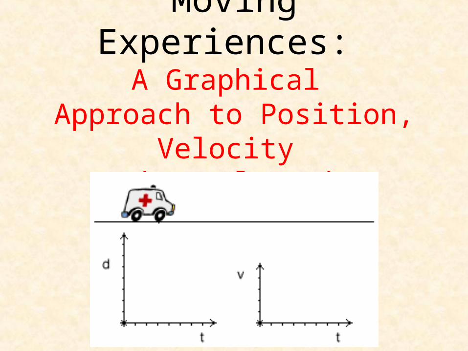
We represent this motion with a

position-time graph, with position on the

vertical axis and time on the horizontal.

Define the object’s average velocity during

the interval t: f ix x

vt

It should be clear that this average

velocity is also the slope of the object’s position-time graph.

xi

xf

ti tf

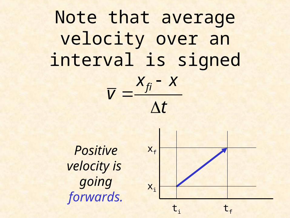
Note that average velocity over an interval is signed

f ix xv

t

Positive velocity is going forwards. xi

xf

ti tf

And the sign of velocity is relative to the position

coordinate systemf ix x

vt

Negative velocity is going

backwards! xf

xi

ti tf

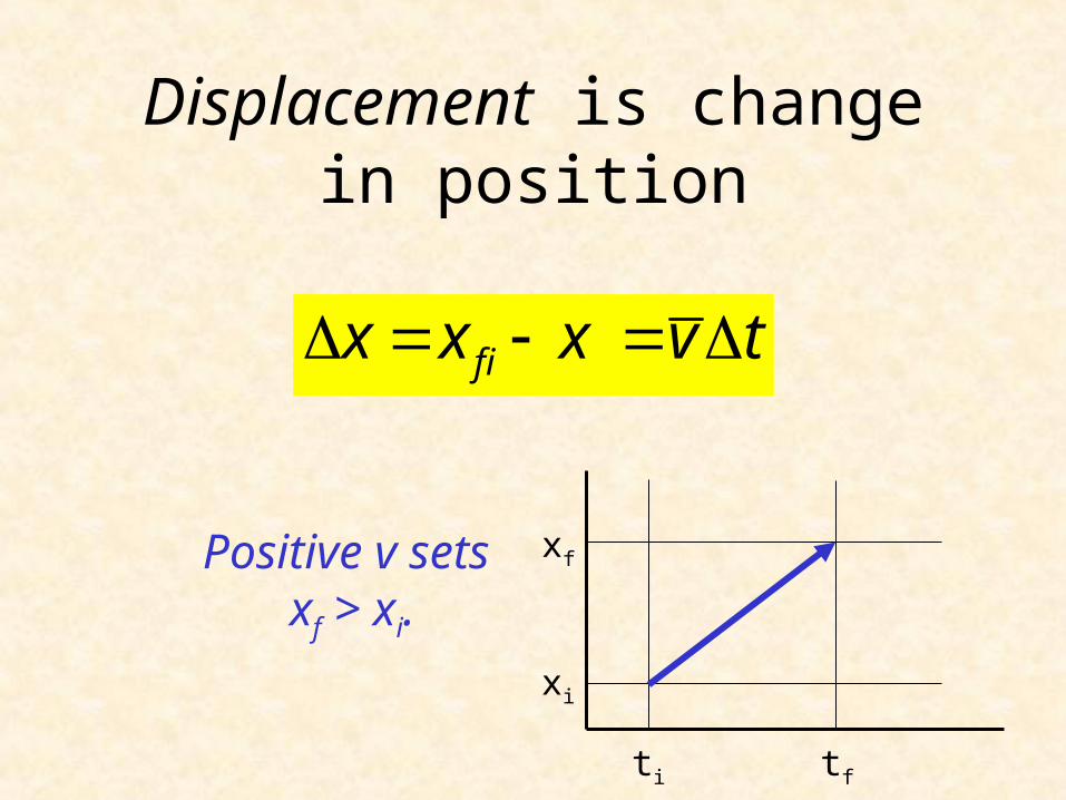
Displacement is change in position

f ix x x v t

Positive v sets xf > xi.

xi

xf

ti tf

Displacement can be negative

Negative v sets xf < xi

xf

xi

ti tf

f ix x x v t

Displacement varies in sign, but distance traveled

does not

f ix x x v t

xf

xi

ti tf

Displacement:

Distance traveled: | | | |f ix x v t

Distance traveled: Same same

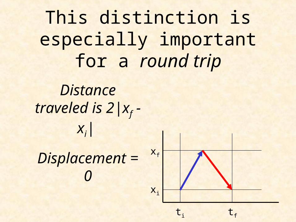
This distinction is especially important for a

round trip

xi

xf

ti tf

Distance traveled is 2|xf - xi|

Displacement = 0

Speed is the magnitude of velocity, which cannot be

negative

xi

xf

ti tf

Round trip speed is 2|xf - xi| (tf – ti)

Displacement = 0

Now its time to

accelerate

Suppose velocity changes at

the constant rate a, such that:

,

i

i

f

f

v va

tor v v a t

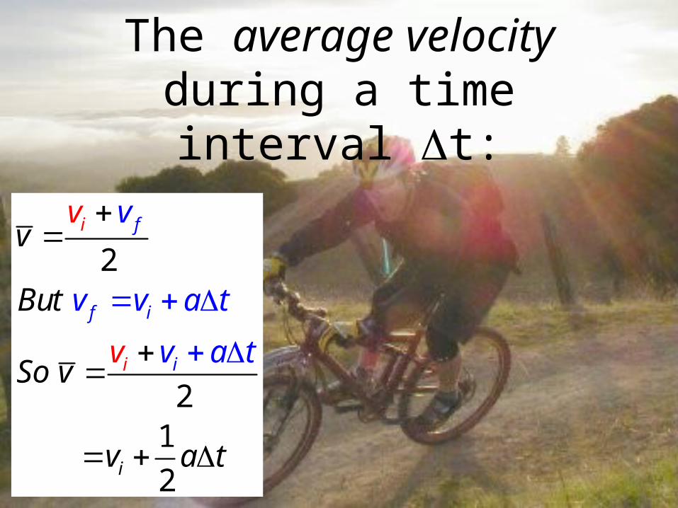
The average velocity during a time interval

t:

2

21

2

f

i

f

i

i

ii

v

But

So

v

v v a t

v av

v a t

v

v t

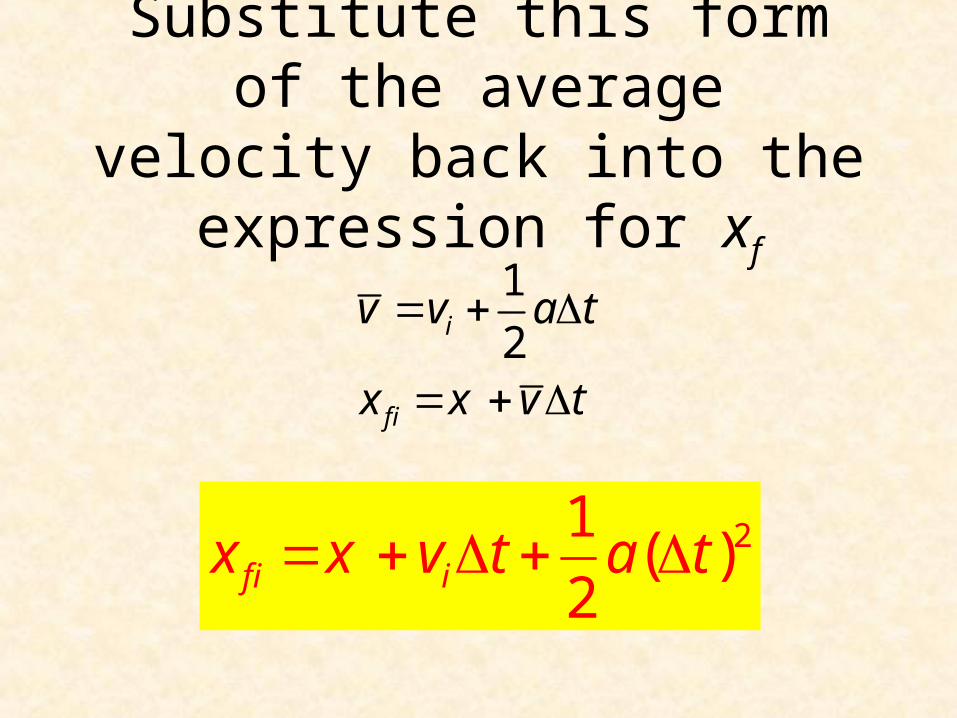
Substitute this form of the average velocity back into

the expression for xf

21( )

2f i ix x v t a t

1

2i

f i

v v a t

x x v t

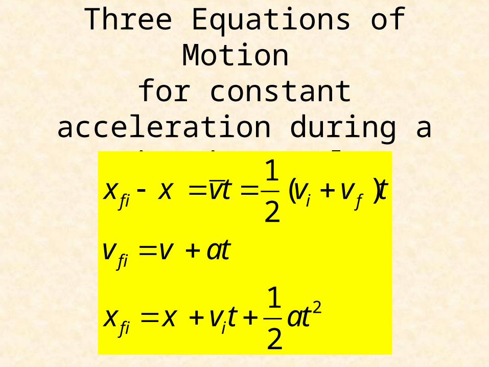
Thus: Three Equations of Motion for constant acceleration during a time interval t

2

1( )

2

1

2

f i i f

f i

f i i

x x vt v v t

v v at

x x v t at

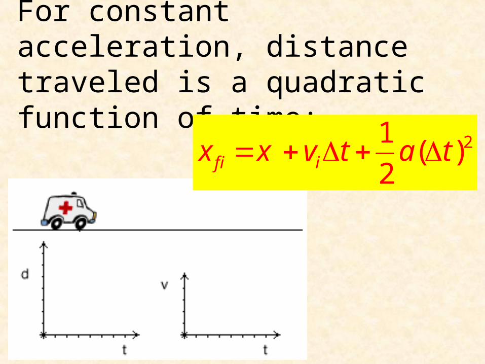
For constant acceleration, distance traveled is a quadratic function of time:

21( )

2f i ix x v t a t

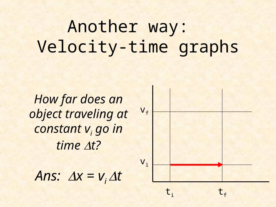
Another way: Velocity-time graphs

vi

vf

ti tf

How far does an object traveling at constant vi go in

time t?

Ans: x = vi t

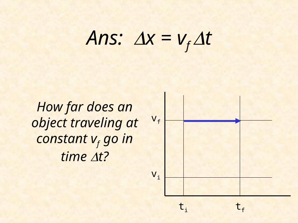
Ans: x = vf t

vi

vf

ti tf

How far does an object traveling at constant vf go in

time t?

x = v t

vi

vf

ti tf

Both distances are numerically equal to the area of the

rectangle of height v and width t.

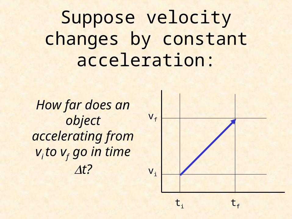
Suppose velocity changes by constant acceleration:

vi

vf

ti tf

How far does an object accelerating from vi to vf go in

time t?

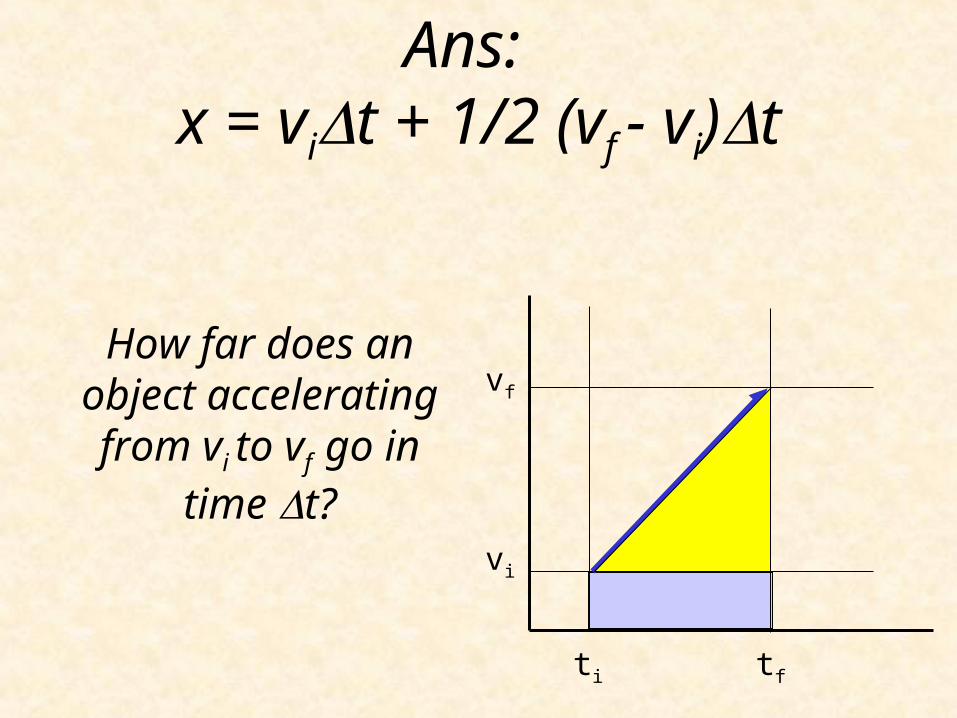
Ans: x = vit + 1/2 (vf - vi)t

vi

vf

ti tf

How far does an object accelerating from vi to

vf go in time t?

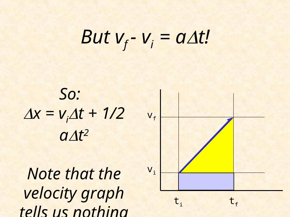
But vf - vi = at!

vi

vf

ti tf

So: x = vit + 1/2 at2

Note that the velocity graph tells

us nothing about the initial xi

These relationships between a function, its slope and the

area below its graph

vi

vf

ti tf

are the key ties between the Physics of

Motion and the Calculus

But we can still produce

one more equation!

One more equation:

2 2:

2

2

f i i f

f i

f i

v v and v v

Multiply v v

But

a t

a t

v

v

t x x x

v

2 2 2f iS v v xao

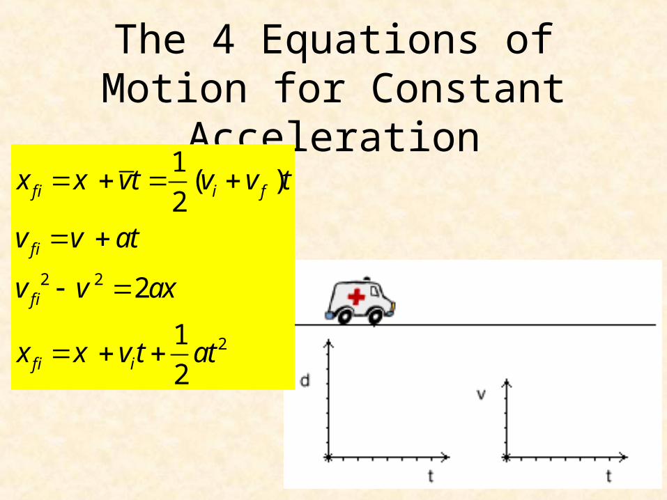
The 4 Equations of Motion for Constant Acceleration

2 2

2

1( )

2

2

1

2

f i i f

f i

f i

f i i

x x vt v v t

v v at

v v ax

x x v t at

The 4 Equations of Motion for Constant Acceleration

2 2

2

1( )

2

2

1

2

f i i f

f i

f i

f i i

x x vt v v t

v v at

v v ax

x x v t at