Moving Average Stochastic Volatility Models with

Application to Inflation Forecast

Joshua C.C. Chan∗

Research School of Economics,Australian National University

May 2013

Abstract

We introduce a new class of models that has both stochastic volatility and movingaverage errors, where the conditional mean has a state space representation. Havinga moving average component, however, means that the errors in the measurementequation are no longer serially independent, and estimation becomes more difficult.We develop a posterior simulator that builds upon recent advances in precision-based algorithms for estimating these new models. In an empirical application in-volving U.S. inflation we find that these moving average stochastic volatility modelsprovide better in-sample fitness and out-of-sample forecast performance than thestandard variants with only stochastic volatility.

Keywords: state space, unobserved components model, precision, sparse, densityforecast

JEL classification codes: C11, C51, C53

∗We thank seminar participants at Monash University, the 6-th Rimini Bayesian EconometricsWorkshop, the 18-th Australasian Macroeconomics Workshop, and Workshop on Empirical Methodsin Macroeconomic Policy Analysis for helpful comments and suggestions. All errors are, of course,our own. Postal address: Research School of Economics, ANU College of Business and Economics,LF Crisp Building 26, The Australian National University, Canberra ACT 0200, Australia. Email:joshua.chan@anu.edu.au. Phone: (+61) 2 612 57358. Fax: (+61) 2 612 50182.

1 Introduction

Since the pioneering works of Box and Jenkins, autoregressive moving average (ARMA)models have become standard tools for modeling and forecasting time series. The theo-retical justification of these ARMA models, as is well-known, is the Wold decompositiontheorem, which states that any zero mean covariance-stationary time series has an in-finite moving average representation. One implication is that any such process can beapproximated arbitrarily well by a sufficiently high order ARMA model. In practice, itis found that simple univariate ARMA models often outperform complex multivariatemodels in forecasting.

However, despite the theoretical justification and empirical success of this class of mod-els, a voluminous literature has highlighted the importance of allowing for time-varyingvolatility in macroeconomic and financial data for estimation and forecasting. StandardARMA models that assume constant variance are seemingly not flexible enough. Oneway to accommodate this time-variation in variance is via the GARCH model (Boller-slev, 1986). For example, Nakatsuma (2000) considers a linear regression model withARMA-GARCH errors. Another popular way to allow for time-varying volatility is viathe stochastic volatility (SV) model (e.g., Taylor, 1994; Kim, Shepherd, and Chib, 1998).The popularity of this approach can be seen through the numerous extensions of thebasic SV setup in recent years, such as the SV models with jump and Student’s t error(Chib, Nardari, and Shephard, 2002), SV with leverage (Jacquier, Polson, and Rossi,2004; Omori, Chib, Shephard, and Nakajima, 2007), SV with asymmetric, heavy-tailederror (Nakajima and Omori, 2012), semiparametric SV models via the Dirichlet processmixture (Jensen and Maheu, 2010), etc., to name but a few examples.

Several recent studies have attempted to bridge these two literatures on ARMA andSV models, and have considered various flexible autoregressive models with stochasticvolatility (e.g., Cogley and Sargent, 2005; Primiceri, 2005; Cogley, Primiceri, and Sargent,2010). But there are few papers that investigate moving average models with SV. Thepurpose of this article is to fill this gap: we introduce a class of models that includes boththe moving average and stochastic volatility components, where the conditional meanprocess has a flexible state space representation. As such, the setup includes a wide varietyof popular specifications as special cases, including the unobserved components and time-varying parameter models. Of course, any invertible MA process can be approximatedby a sufficiently high order AR model. In practice, however, forecasts based on theseAR models—since they have many parameters to estimate—often compare poorly toparsimonious ARMA models (e.g., Stock and Watson, 2007; Athanasopoulos and Vahid,2008). In our empirical work that involves quarterly inflation, we find that there issubstantial support for the proposed models against their counterparts with only SV.The forecasting results suggest that addition of the MA component further improves theforecast performance of standard SV models, particularly at short forecast horizons.

A second contribution of this paper is to develop an efficient Markov chain Monte Carlo(MCMC) sampler for estimating this class of models. Since the conditional mean process

2

has a state space form, estimation might appear to be straightforward. However, underour models the errors in the measurement equation are no longer serially independentdue to the presence of the MA component. As such, application of Kalman filter-basedmethods would first require a suitable transformation of the data to make the errorsserially independent. Instead of using the Kalman filter, we take a different approach: weextend previous work on precision-based algorithms for state space models in Chan andJeliazkov (2009) and McCausland, Miller, and Pelletier (2011), which are shown to bemore efficient than Kalman filter-based methods. The idea of exploiting banded precisionmatrix can be traced back to Fahrmeir and Kaufmann (1991); see also Rue, Martino, andChopin (2009) and Ruiz-Cardenas, Krainski, and Rue (2012). By exploiting the sparsestructure of the covariance matrix of the observations, we develop an easy and fast methodfor estimating these new models.

A third contribution involves a substantive empirical application on modeling and fore-casting U.S. quarterly consumer price index (CPI) inflation. A vast literature on this topichas emerged over the last two decades; recent studies include Koop and Potter (2007),Stock and Watson (2007, 2010), Cogley and Sbordone (2008), Cogley et al. (2010), Clarkand Doh (2011), Korobilis (2012), Koop and Korobilis (2012), among many others. Onekey finding in this literature is that both persistence and volatility in the inflation processhave changed considerably over time. In particular, inflation volatility decreased gradu-ally from the great inflation of the 1970s and throughout the great moderation, until itincreased again and peaked at the aftermath of the global financial crisis. Empirically,it is often found that models with stochastic volatility provide substantially better pointand density forecasts than those obtained from constant error variance models (e.g., Clarkand Doh, 2011; Chan, Koop, Leon-Gonzalez, and Strachan, 2012a).

Another key finding in this literature is that for forecasting inflation, both at short andlong horizons, it is often difficult to improve upon univariate models using only informa-tion in observed inflation (e.g., Stock and Watson, 2007, 2010; Chan et al., 2012a). Onereason for this lack of predictive power of a wide range of seemingly relevant variables—such as unemployment rate and GDP growth—might be because variables useful forforecasting change over time (e.g., oil price might be an important predictor for inflationin the 1970s but is less important in the 2000s) and/or over business cycle (e.g., somevariables may predict well in expansions but not in recessions). In fact, Koop and Ko-robilis (2012) find evidence that the set of relevant predictors for inflation does changeover time. Given these findings, we consider univariate time series models using onlyinformation in observed inflation. Additional explanatory variables, of course, can beincorporated if desired.

We focus on univariate MA-SV models in this paper, partly because for our empiricalwork these models are sufficient. We note that the univariate framework developed herecan be used to construct multivariate models in a straightforward manner. For example,in the multivariate SV models of Chib, Nardari, and Shephard (2006), SV is induced bya number of latent factors, each of which follows an independent univariate SV process.In this setup, we can, for example, replace the SV process with the univariate MA-SV

3

process introduced in this paper to construct a multivariate SV model with autocorrelatederrors. We leave the multivariate case for future research.

The rest of this article is organized as follows. In Section 2 we introduce the generalframework, and discuss how this state space form includes a variety of popular specifi-cations as special cases. Section 3 develops an efficient posterior simulator to estimatethis new class of models. Section 4 presents empirical results for modeling and forecast-ing U.S. CPI inflation. In the last section we conclude our findings and discuss futureresearch direction.

2 Moving Average Stochastic Volatility Models

The general framework we consider is the following q-th-order moving average model withstochastic volatility:

yt = µt + εyt , (1)

εyt = ut + ψ1ut−1 + · · ·+ ψqut−q, ut ∼ N (0, eht), (2)

ht = µh + φh(ht−1 − µh) + εht , εht ∼ N (0, σ2h), (3)

where we assume |φh| < 1. The errors ut and εht are independent of each other for allleads and lags. We further assume that u0 = u−1 = · · · = u−q+1 = 0. One can, of course,treat these initial error terms as parameters if desired, and the estimation proceduresdiscussed in the next section can be easily extended to allow for this possibility. Fortypical situations where T ≫ q, whether these errors are modeled explicitly or not makeslittle difference in practice.

Let µ = (µ1, . . . , µT )′, h = (h1, . . . , hT )

′ and ψ = (ψ1, . . . , ψq)′. Then, it is easy to see

that the conditional variance of yt is given by

Var(yt |µ,ψ,h) = eht + ψ21eht−1 + · · ·+ ψ2

qeht−q .

In other words, the conditional variance of yt is time-varying through two channels: it isa moving average of the q + 1 most recent variances eht , . . . , eht−q , and the log-volatilityht in turn evolves according to the stationary AR(1) process in (3). Unlike the standardSV models, yt is serially correlated even after conditioning on the states. In fact, itsconditional autocovariances are given by

Cov(yt, yt−j |µ,ψ,h) =

∑q−j

i=0 ψi+jψieht−i, for j = 1, . . . , q,

0, for j > q,

where ψ0 = 1. It is interesting to note that due to the presence of the log-volatility ht,the autocovariances of yt are also time-varying.1

1On the other hand, the marginal variance and autocovariances of yt unconditional on h do not seemto have closed-form expressions.

4

Now, by choosing a suitable conditional mean process µt, the model in (1)–(3) includesa variety of popular specifications, such as:

1. the autoregressive model:

µt = φ0 + φ1yt−1 + · · ·+ φpyt−p;

2. the linear regression model:

µt = β0 + β1x1t + · · ·+ βkxkt,

where xt = (x1t, . . . , xkt) is a vector of explanatory variables;

3. the unobserved components model:

µt = τt,

τt = τt−1 + ετt , ετt ∼ N (0, σ2τ );

4. the time-varying parameter model:

µt = β0t + β1tx1t + · · ·+ βktxkt,

βt = βt−1 + εβt , ε

βt ∼ N (0,Σβ),

where βt = (β0t, β1t, . . . , βkt)′.

Some other flexible time-varying models recently introduced also fall within this generalframework. Examples include an autoregressive unobserved components model discussedin Clark and Doh (2011), as well as various bounded trend inflation models proposedin Chan, Koop, and Potter (2012b). The framework in (1)–(3) is a natural extension ofthe standard stochastic volatility setting. In particular, the latter is a special case of thisgeneral framework with ψ1 = · · · = ψq = 0. For identification purposes, we assume theusual invertiblilty conditions, i.e., the roots of the characteristic polynomial associatedwith the MA coefficients are all outside the unit circle.

It is well known that moving average models have a state space representation, andthe likelihood function can be evaluated using the Kalman filter (Harvey, 1985). Thisapproach can be slow, however, especially when we need to make tens of thousandsfunctional evaluations of the likelihood in the MCMC algorithm. We therefore introducein the next section a direct way to evaluate the likelihood function. By utilizing fast sparsematrix routines, the new approach is simple and easy to program. Another complicationin our setting is that the MA component induces serial dependence in observations.Consequently, in order to apply conventional Kalman filter-based methods to simulatethe states, one would first need to transform the data so that the errors in the newmeasurement equation are serially independent (e.g., one such transformation is suggestedin Chib and Greenberg, 1994). Instead of using Kalman filter, we introduce a directapproach that builds upon previous work on precision-based algorithms in Chan andJeliazkov (2009) for fitting this new class of models. McCausland et al. (2011) providea careful comparison between Kalman-filter based and precision-based algorithms, andshow that the latter algorithms are substantially more efficient.

5

3 Estimation

We introduce a direct approach for estimating the class of models in (1)–(3) that exploitsthe special structure of the problem, particularly that the covariance matrix of the jointdistribution for y = (y1, . . . , yT )

′ is sparse, i.e., it contains only a few non-zero elements.We first introduce a fast and simple way to evaluate the likelihood function that is usefulfor both maximum likelihood and Bayesian estimation. It is followed by a detailed discus-sion on a new posterior simulator for estimating the log-volatilities and the parametersin the conditional mean process.

3.1 Likelihood Evaluation

To obtain the likelihood function, we first derive the joint distribution of the observationsy = (y1, . . . , yT )

′. To this end, we rewrite (1)–(2) in matrix notations:

y = µ+Hψu, (4)

where µ = (µ1, . . . , µT )′, u = (u1, . . . , uT )

′ ∼ N (0,Sy), Sy = diag(eh1, . . . , ehT ), and Hψ

is a T × T lower triangular matrix with ones on the main diagonal, ψ1 on first lowerdiagonal, ψ2 on second lower diagonal, and so forth. For example, for q = 2, we have

Hψ =

1 0 0 0 · · · 0ψ1 1 0 0 · · · 0ψ2 ψ1 1 0 · · · 00 ψ2 ψ1 1 · · · 0...

. . .. . .

. . ....

0 0 · · · ψ2 ψ1 1

.

It is important to note that in general Hψ is a banded T × T matrix that containsonly (T − q/2)(q + 1) < T (q + 1) non-zero elements, which is substantially less thanT 2 for typical applications where T ≫ q. This special structure can be exploited tospeed up computation. For instance, obtaining the Cholesky decomposition of a bandedT × T matrix with fixed bandwidth involves only O(T ) operations (e.g., Golub andvan Loan, 1983, p.156) as opposed to O(T 3) for a full matrix of the same size. Similarcomputational savings can be generated in operations such as multiplication, forward andbackward substitution by using block-banded or sparse matrix algorithms. These bandedand sparse matrix algorithms are implemented in standard packages such as Matlab,Gauss and R.

Now, by a simple change of variable, it follows from (4) that

(y |ψ,µ,h) ∼ N (µ,Ωy),

where h = (h1, . . . , hT )′, Ωy = Hψ Sy H

′

ψ. Since Sy = diag(eh1 , . . . , ehT ) is a diagonalmatrix, and Hψ is a lower triangular sparse matrix, the product Ωy is sparse. In fact,

6

it is a banded matrix with only a narrow band of non-zero elements around the maindiagonal. Moreover, since |Hψ| = 1 for any ψ = (ψ1, . . . , ψq)

′, we have |Ωy| = |Sy| =

exp(∑T

t=1 ht

). The log joint density of y is therefore given by

log p(y |ψ,µ,h) = −T

2log(2π)−

1

2

T∑

t=1

ht −1

2(y − µ)′Ω−1

y(y− µ). (5)

It is important to realize that one need not obtain the T ×T inverse matrix Ω−1y

in orderto evaluate the log density in (5)—it would involve O(T 3) operations. Instead, it can becomputed in three steps, each of which requires only O(T ) operations. To this end, weintroduce the following notations: given a lower (upper) triangular T × T non-singularmatrixA and a T×1 vector c, letA\c denote the unique solution to the triangular systemAx = c obtained by forward (backward) substitution, i.e., A\c = A−1c. Now, we firstobtain the Cholesky decomposition Cy of the banded matrix Ωy such that CyC

′

y= Ωy,

which involves only O(T ) operations. Then compute

x1 = C′

y\(Cy\(y− µ))

by forward followed by backward substitution, each of which requires O(T ) operationssince Cy is also banded. By definition,

x1 = C−1′

y(C−1

y(y − µ)) = (CyC

′

y)−1(y − µ) = Ω−1

y(y − µ).

Finally, compute

x2 = −1

2(y − µ)′x1 = −

1

2(y − µ)′Ω−1

y(y − µ),

which gives the quadratic term in (5). Thus, given µ, ψ and h, one can efficiently evaluatethe likelihood function without the need of the Kalman filter.

3.2 Posterior Analysis

Now, we discuss an efficient posterior sampler for estimating the MA-SV model in (1)–(3).To keep the discussion concrete, we consider in particular the unobserved componentsspecification; estimation for other conditional mean processes follows similarly. Specifi-cally, the measurement equation is given by (4) with µ = τ = (τ1, . . . , τT )

′, whereas thetransition equations are

τt = τt−1 + ετt , ετt ∼ N (0, σ2τ ),

ht = µh + φh(ht−1 − µh) + εht , εht ∼ N (0, σ2h),

with |φh| < 1. The transition equation for τt is initialized with τ1 ∼ N (τ0, σ20τ ), where τ0

and σ20τ are some known constants. In particular, we set τ0 = 0. Moreover, the transition

equation for ht is initialized with h1 ∼ N (µh, σ2h/(1− φ2

h)).

7

We assume independent priors for ψ, σ2τ , µh, φh and σ2

h, i.e., p(ψ, σ2τ , µh, φh, σ

2h) =

p(ψ)p(σ2τ )p(µh)p(φh)p(σ

2h). For ψ, we consider a multivariate normal prior with sup-

port in the region where the invertibility conditions on ψ hold. As for other parameters,we assume the following independent priors:

σ2τ ∼ IG(ντ , Sτ), µh ∼ N (µh0, Vµh), φh ∼ N (φh0, Vφh)1l(|φh| < 1), σ2

h ∼ IG(νh, Sh),

where IG denotes the inverse-gamma distribution. Note that we impose the stationaritycondition |φh| < 1 through the prior on φh. Then posterior draws can be obtained bysequentially sampling from:2

1. p(τ |y,h,ψ, σ2τ );

2. p(h |y, τ ,ψ, σ2h, µh, φh);

3. p(ψ, σ2h, σ

2τ |y, τ ,h, µh, φh) = p(ψ |y, τ ,h) p(σ2

h |h, µh, φh) p(σ2τ | τ );

4. p(µh |h, σ2h, φh);

5. p(φh |h, µh, σ2h).

We first discuss an efficient way to sample from p(τ |y,h,ψ, σ2τ ). First note that by

pre-multiplying (4) by H−1ψ , we have

y = τ + u,

where y = H−1ψ y and τ = H−1

ψ τ . In other words, the log density for y is

log p(y |ψ, τ ,h) ∝ −1

2

T∑

t=1

ht −1

2(y− τ )′S−1

y(y − τ ), (6)

where Sy = diag(eh1, . . . , ehT ). Hence it is more convenient to work with τ instead of theoriginal parameterization τ . Once we have a draw for τ , we simply pre-multiply it byHψ to get a draw for τ .

Next, we derive the prior density for τ . To this end, we first obtain the prior density forτ . Rewrite the transition equation for τt in matrix notations:

Hτ = ετ ,

where ετ = (ετ1, . . . , ετT )

′ ∼ N (0,Sτ ), Sτ = diag(σ20τ , σ

2τ , . . . , σ

2τ ), and H is the first

difference matrix

H =

1 0 0 · · · 0−1 1 0 · · · 00 −1 1 · · · 0...

. . ....

0 0 · · · −1 1

.

2Matlab codes for estimating this unobserved components MA-SV model are available athttp://people.anu.edu.au/joshua.chan/.

8

That is, (τ | σ2τ ) ∼ N (0,Ωτ ), where Ω−1

τ = H′S−1τ H. Recall that σ2

0τ is the variance forthe initial underlying trend τ1, and is assumed to be a fixed hyper-parameter (althoughit is straightforward to treat it as a parameter).

It is important to realize that in this case the precision matrix Ω−1τ is sparse. Now,

by a simple change of variable, we have (τ | σ2τ ) ∼ N (0,H−1

ψ ΩτH−1′

ψ ). Noting that

|H| = |Hψ| = 1 and |Ωτ | = σ20τ (σ

2τ )T−1, the log prior density for τ is therefore given by

log p(τ | σ2τ ) ∝ −

T − 1

2log σ2

τ −1

2τ′H′

ψΩ−1τ Hψτ , (7)

Combining (6) and (7), and using standard results from linear regression (see, e.g., Koop,2003), we obtain the log conditional density log p(τ | y,h,ψ, σ2

τ ) as follows:

log p(τ | y,h,ψ, σ2τ ) ∝−

1

2(y − τ )′S−1

y(y− τ )−

1

2τ′H′

ψΩ−1τ Hψτ

∝−1

2(τ ′(S−1

y+H′

ψΩ−1τ Hψ)τ − 2τ ′S−1

yy)

∝−1

2(τ − τ )′D−1

τ(τ − τ ),

where Dτ = (S−1y

+H′

ψΩ−1τ Hψ)

−1, and τ = DτS−1yy. That is,

(τ | y,h,ψ, σ2τ ) ∼ N (τ ,Dτ ).

Since N (τ ,Dτ ) is typically high dimensional, sampling from it using a brute-force ap-proach is time-consuming. Here we adopt the precision-based sampling method in Chanand Jeliazkov (2009) to obtain draws from N (τ ,Dτ ) efficiently. To proceed, first notethat the precision matrix D−1

τ = (S−1y

+H′

ψΩ−1τ Hψ) is sparse. Thus τ can be computed

quickly using the same approach for evaluating the likelihood function discussed earlier:obtain the Cholesky decomposition Cτ of D−1

τ , and compute

τ = C′

τ\(Cτ\(S−1yy))

by forward and backward substitution. A draw from N (τ ,Dτ ) can now be obtained asfollows: sample T independent standard normal draws z ∼ N (0, I) and return

τ = τ +C′

τ\z.

Since τ is an affine transformation of a normal random vector, it is also a normal randomvector. It is easy to check that its expectation is τ and its covariance matrix is

C−1′

τ C−1τ = (CτC

′

τ )−1 = Dτ

as desired. Finally, given the draw τ ∼ N (τ ,Dτ ), return τ = Hψτ .

In Step 2 of the MCMC sampler, we sample from p(h |y, τ ,ψ, σ2h, µh, φh). To proceed,

first define y∗ = H−1ψ (y − τ ). It follows from (4) that y∗ = u ∼ N (0,Sy), where Sy =

diag(eh1 , . . . , ehT ). With this transformation, the auxiliary mixture sampling approach in

9

Kim, Shepherd, and Chib (1998) can be applied to draw h efficiently; see also Koop andKorobilis (2010), p. 308–310, for a textbook treatment. Note that in Kim et al. (1998), aforward-backward smoothing algorithm is used; here it is replaced by the precision-basedsampler.

For Step 3, note that ψ, σ2h, and σ2

τ are conditionally independent given y, τ , and h.Hence, we can sample each sequentially. Given the prior p(ψ), it follows from (5) that

log p(ψ |y, τ ,h) ∝ log p(ψ) + log p(y |ψ, τ ,h)

∝ log p(ψ)−1

2y∗

′

S−1yy∗,

where we use the transformation y∗ = H−1ψ (y − τ ). Hence, log p(ψ |y, τ ,h) can be

quickly evaluated for any ψ given y, τ and h using the method discussed in the previoussection. Since in typical applications ψ is low dimensional—only a few moving averageterms are needed—one can maximize log p(ψ |y, τ ,h) numerically and obtain the mode

and the negative Hessian evaluated at the mode, denoted as ψ andK, respectively. Then,draws from p(ψ |y, τ ,h) are obtained using an independence-chain Metropolis-Hastings

step with proposal density N (ψ,K−1), for example. When ψ is high dimensional, onecan avoid the high-dimensional numerical maximization by implementing, e.g., variousadaptive MCMC samplers discussed in Andrieu and Thoms (2008).

Next, both p(σ2h |h, µh, φh) and p(σ

2τ | τ ) are inverse-gamma densities, and can therefore

be sampled using standard methods. In fact, we have

(σ2τ | τ ) ∼ IG

(ντ + (T − 1)/2, Sτ

), (σ2

h |h, µh, φh) ∼ IG(νh + T/2, Sh

),

where Sτ = Sτ +∑T

t=2(τt − τt−1)2/2 and Sh = Sh + [(1− φ2

h)(h1 − µh)2 +

∑T

t=2(ht − µh−φh(ht−1 − µh))

2]/2. Lastly, Steps 4 and 5 are standard and can be performed, e.g., asdescribed in Kim et al. (1998) by simply changing the priors.

We note that the estimation for other conditional mean processes can be implementedanalogously; we provide the estimation details for the autoregressive MA-SV model inthe appendix.

3.3 Computation Efficiency

In this section we briefly discuss some computation issues and the scalability of thealgorithm introduced in the previous section. In a typical finance application, for example,one might have time series with thousands of observations. It is therefore important thatthe estimation method can handle data with large T . In what follows, we discuss thecomputational complexity of the proposed posterior sampler as T gets large. Again, forconcreteness we consider in particular the unobserved components model.

First, the conditional distribution p(τ |y,h,ψ, σ2τ ) is Gaussian, and draws from this distri-

bution can be obtained exactly using the precision-based method. In particular, obtaining

10

a draw requires the Cholesky decomposition of the banded precision matrix, as well as afew forward/backward substitutions. Each of these operations involves only O(T ) oper-ations. In Step 2 of the posterior sampler, we first transform the data y∗ = H−1

ψ (y− τ ),which involves O(T ) operations as Hψ is a banded matrix. Then, we directly apply theauxiliary mixture sampling of Kim et al. (1998). Hence, this step is as efficient as thecorresponding step in standard SV models.

Next, in Step 3 of the posterior sampler, the conditional distribution p(ψ |y, τ ,h) is non-

standard, and we numerically maximize log p(ψ |y, τ ,h) to obtain the mode ψ and K,the negative Hessian evaluated at the mode. We then implement a Metropolis-Hastingsstep with the proposal density N (ψ,K−1). Evaluation of p(ψ |y, τ ,h) is done using themethod described in Section 3.1, which again requires O(T ) operations. This step issufficiently efficient in typical applications where ψ is low dimensional. When ψ is highdimensional, one can avoid the high-dimensional numerical maximization by implement-ing, e.g., adaptive MCMC samplers such as those discussed in Andrieu and Thoms (2008).Lastly, the remaining steps—drawing from p(σ2

h |h, µh, φh), p(σ2τ | τ ), p(µh |h, σ

2h, φh) and

p(φh |h, µh, σ2h)—require trivial computation efforts and can be done quickly even when

T is large.

2006 2007 2008 2009 2010 2011−8

−6

−4

−2

0

2

4

6

8

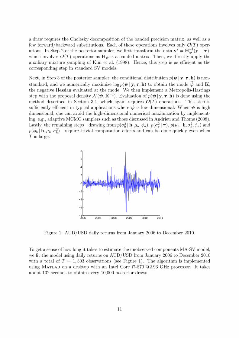
Figure 1: AUD/USD daily returns from January 2006 to December 2010.

To get a sense of how long it takes to estimate the unobserved components MA-SV model,we fit the model using daily returns on AUD/USD from January 2006 to December 2010with a total of T = 1, 303 observations (see Figure 1). The algorithm is implementedusing Matlab on a desktop with an Intel Core i7-870 @2.93 GHz processor. It takesabout 132 seconds to obtain every 10,000 posterior draws.

11

4 Modeling and Forecasting U.S. Inflation Rate

Now we use the proposed MA-SV models to analyze the behavior of U.S. quarterly CPIinflation, and contrast the results with those obtained from the standard variants withonly stochastic volatility. In addition, we also compare the forecast performance of thetwo classes of models at various forecast horizons. Since allowing for stochastic volatilityis found to be empirically important, unless stated otherwise, models considered in thissection all have stochastic volatility in the measurement equation.

4.1 Competing Models

We consider four popular specifications for modeling inflation, and for each we have twoversions: with and without the MA component. The primary goal of this exercise is notto find the best model per se. Rather, our objective is to investigate if the addition ofthe MA component improves model-fit and forecast performance, and how it affects theestimates of the states and other parameters of interest. The first specification is theunobserved components model, which we reproduce here for convenience:

yt = τt + ut, ut ∼ N (0, eht),

τt = τt−1 + ετt , ετt ∼ N (0, σ2τ),

ht = µh + φh(ht−1 − µh) + εht , εht ∼ N (0, σ2h).

We refer to this version of unobserved components model as the UC model. Stock andWatson (2007) extend this specification to include stochastic volatility in the transitionequation for the underlying trend τt. Specifically, the variance for ετt—instead of beingfixed to be a constant—is allowed to be time-varying: ετt ∼ N (0, egt). The log-volatilitygt, in turn, evolves as a stationary AR(1) process:3

gt = µg + φg(gt−1 − µg) + εgt , εgt ∼ N (0, σ2g),

where |φg| < 1. This version of unobserved components model, where both the mea-surement and transition equations have stochastic volatility, is referred to as the UCSVmodel. The final two specifications are autoregressive models:

yt = φ0 + φ1yt−1 + · · ·+ φpyt−p + ut,

where ut has the same stochastic volatility specification as before. In addition, we imposethe conditions that the roots of the characteristic polynomial associated with the ARcoefficients all lie outside the unit circle, so that the AR process is stationary. We considertwo lag lengths p = 1 and p = 2, and we refer them as AR(1) and AR(2) respectively.

For each of the four models—UC, UCSV, AR(1) and AR(2)—we include the MA-SVvariants as specified in (1)–(2), and we refer them asUC-MA,UCSV-MA,AR(1)-MA

3In Stock and Watson (2007) the stochastic volatilities ht and gt evolve as random walks, which maybe viewed as a limiting case considered here with φg = φh = 1.

12

and AR(2)-MA respectively. For these models with the moving average components, weset q, the number of moving average terms, to be one. Empirical evidence supporting thischoice will be presented in Section 4.3. We summarize all eight specifications in Table 1.

Table 1: A list of competing models.

Model DescriptionUC unobserved components modelUC-MA same as UC but with an MA(1) componentUCSV same as UC but the state equation for τt has SVUCSV-MA same as UCSV but with an MA(1) componentAR(1) autoregressive model with 1 lagAR(1)-MA same as AR(1) but with an MA(1) componentAR(2) autoregressive model with 2 lagsAR(2)-MA same as AR(2) but with an MA(1) componentUC-MA-NoSV same as UC-MA but without SVAR(1)-MA-NoSV same as AR(1)-MA but without SVAR(2)-MA-NoSV same as AR(2)-MA but without SV

In the forecasting exercise, we also include three additional models without stochasticvolatility for comparison. Specifically, UC-MA-NoSV is the same as UC-MA, but theerror term in the measurement equation ut now has constant variance: ut ∼ N (0, σ2

y).The models AR(1)-MA-NoSV and AR(2)-MA-NoSV are defined similarly.

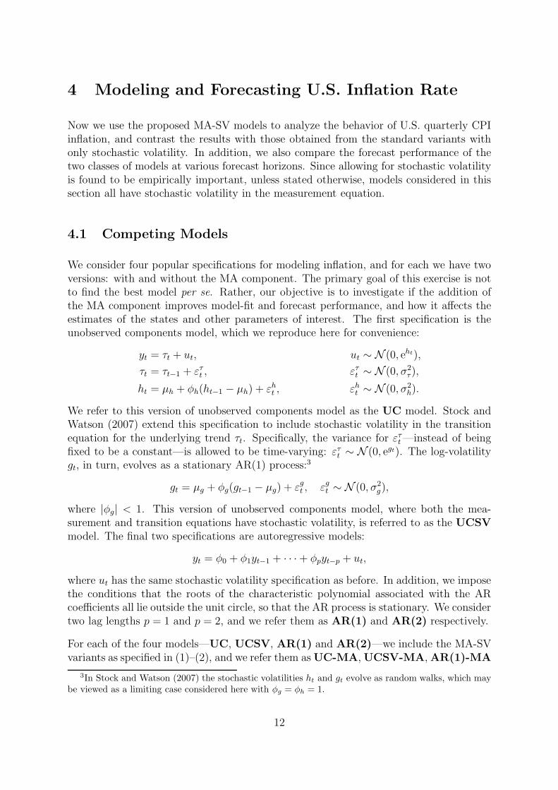
4.2 Data and Priors

The data consist of U.S. quarterly CPI inflation from 1947Q1 to 2011Q3. More specifi-cally, given the quarterly CPI figures zt, we use yt = 400 log(zt/zt−1) as the CPI inflation.A plot of the data is given in Figure 2. For easy comparison, we choose broadly simi-lar priors across models. In particular, we use exactly the same priors for the commonmodel parameters in each pair of models with and without the MA component. For theMA coefficient ψ1, we assume the truncated normal prior ψ1 ∼ N (ψ0, Vψ)1l(|ψ1| < 1) sothat the MA process is invertible. We set ψ0 = 0 and Vψ = 1. The prior distributionthus centers around 0 and has support within the interval (−1, 1). Given the large priorvariance, it is also relatively non-informative.

As discussed in Section 3.2, we assume independent inverse-gamma priors for σ2τ and σ2

h:σ2τ ∼ IG(ντ , Sτ) and σ2

h ∼ IG(νh, Sh). We choose relatively small—hence relatively non-informative—values for the degrees of freedom parameters: ντ = νh = 10. For the scaleparameters, we set Sτ = 0.18 and Sh = 0.45. These values imply E σ2

τ = 0.1412 and E σ2h =

0.2242. The chosen prior means reflect the desired smoothness of the corresponding statetransition, and are comparable to those used in previous studies, such as Chan et al.(2012b) and Stock and Watson (2007). As for µh and φh, their priors are respectively

13

normal and truncated normal: µh ∼ N (µh0, Vµh) and φh ∼ N (φh0, Vφh)1l(|φh| < 1), withµh0 = 0, Vµh = 5, φh0 = 0.9 and Vφh = 1.

1950 1960 1970 1980 1990 2000 2010−10

−5

0

5

10

15

20

Figure 2: U.S. quarterly CPI inflation from 1947Q1 to 2011Q3.

For the models UCSV and UCSV-MA where both the measurement and state equa-tions have stochastic volatility, we follow Stock and Watson (2007) and fix σ2

h and σ2g .

In particular, we set σ2h = σ2

g = 0.2242. For the autoregressive models, we assume atruncated normal prior for the AR coefficients restricted to the stationary region Aφ:φ ∼ N (φ0,Vφ)1l(φ ∈ Aφ), where φ = (φ0, φ1)

′ under the AR(1) and AR(1)-MAmodels, and φ = (φ0, φ1, φ2)

′ under the AR(2) and AR(2)-MA models. Further we setφ0 = 0 and Vφ = 5× I. Finally, for the three models without stochastic volatility—UC-MA-NoSV, AR(1)-MA-NoSV and AR(2)-MA-NoSV—the error variance of themeasurement equation σ2

y is assumed to have an inverse-gamma prior σ2y ∼ IG(νy, Sy)

with νy = 10 and Sy = 9. This implies E σ2y = 1, which is comparable to the stochas-

tic volatility specifications where the prior mean for µh, the unconditional mean of thelog-volatility ht, is µh0 = 0 (and hence exp(µh0) = 1).

4.3 Full Sample Estimation Results

We present in this section the empirical results for the first eight models listed in Table 1,obtained using the full sample from 1947Q1 to 2011Q3. All the posterior moments andquantiles are based on 50,000 draws from the MCMC algorithm introduced in Section 3.2after a burnin period of 5,000.

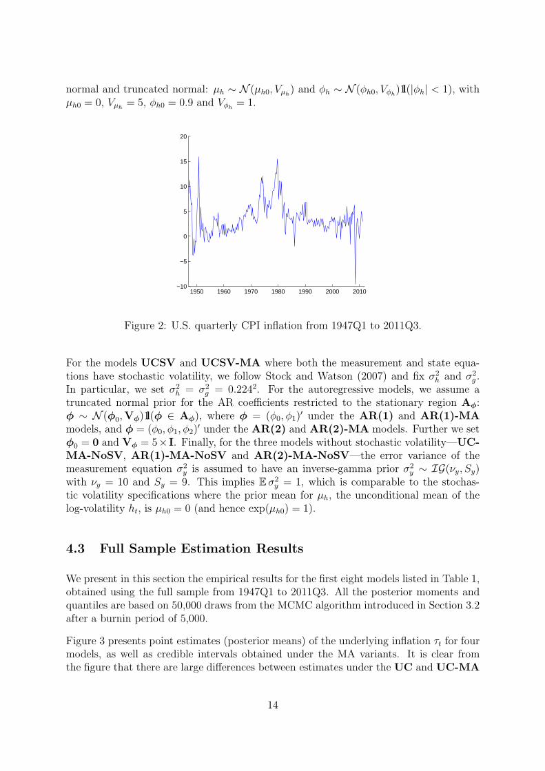
Figure 3 presents point estimates (posterior means) of the underlying inflation τt for fourmodels, as well as credible intervals obtained under the MA variants. It is clear fromthe figure that there are large differences between estimates under the UC and UC-MA

14

models. In particular, by allowing for an extra channel for persistence through the movingaverage errors, the latter model produces much smoother estimates, which are more inline with the notion of a smooth, gradually changing underlying inflation. This finding isbroadly consistent with those reported in earlier studies, such as Clark and Doh (2011)and Chan et al. (2012b), who also find that by explicitly modeling short-run dynamicsone often obtains smoother, more reasonable, underlying inflation estimates.

1950 1960 1970 1980 1990 2000 20100

2

4

6

8

10

1950 1960 1970 1980 1990 2000 2010−5

0

5

10

15

UCSV−MAUCSV5%−tile95%−tile

UC−MAUC5%−tile95%−tile

Figure 3: Posterior estimates and quantiles for τt under the UC, UC-MA, UCSV andUCSV-MA models. The posterior quantiles are obtained under the MA variants.

On the other hand, the underlying inflation estimates for the UCSV and UCSV-MAmodels are very similar, except for the early sample where those for the former appearto be more erratic. By allowing the volatility in the transition equation for τt to be time-varying, the model attributes much of the variation in observed inflation to variation inτt, with the consequence that it traces closely the actual inflation. As such, the movingaverage errors in the measurement equation play a lesser role in channeling the short-rundynamics of the series. The erratic underlying inflation estimates, which change rapidly inshort periods, cast doubt on the overall appropriateness of theUCSV model. Regardless,for our purpose it suffices to note that the MA component does help to obtain smootherestimates for the underlying inflation, though to a lesser extent than in the UC model.

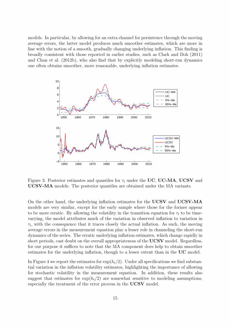
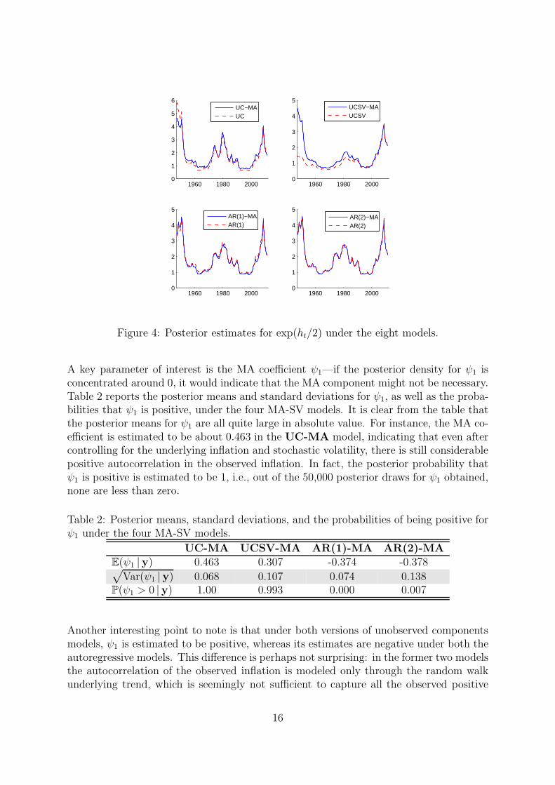
In Figure 4 we report the estimates for exp(ht/2). Under all specifications we find substan-tial variation in the inflation volatility estimates, highlighting the importance of allowingfor stochastic volatility in the measurement equation. In addition, these results alsosuggest that estimates for exp(ht/2) are somewhat sensitive to modeling assumptions,especially the treatment of the error process in the UCSV model.

15

1960 1980 20000

1

2

3

4

5

6

1960 1980 20000

1

2

3

4

5

1960 1980 20000

1

2

3

4

5

1960 1980 20000

1

2

3

4

5

UC−MAUC

UCSV−MAUCSV

AR(1)−MAAR(1)

AR(2)−MAAR(2)

Figure 4: Posterior estimates for exp(ht/2) under the eight models.

A key parameter of interest is the MA coefficient ψ1—if the posterior density for ψ1 isconcentrated around 0, it would indicate that the MA component might not be necessary.Table 2 reports the posterior means and standard deviations for ψ1, as well as the proba-bilities that ψ1 is positive, under the four MA-SV models. It is clear from the table thatthe posterior means for ψ1 are all quite large in absolute value. For instance, the MA co-efficient is estimated to be about 0.463 in the UC-MA model, indicating that even aftercontrolling for the underlying inflation and stochastic volatility, there is still considerablepositive autocorrelation in the observed inflation. In fact, the posterior probability thatψ1 is positive is estimated to be 1, i.e., out of the 50,000 posterior draws for ψ1 obtained,none are less than zero.

Table 2: Posterior means, standard deviations, and the probabilities of being positive forψ1 under the four MA-SV models.

UC-MA UCSV-MA AR(1)-MA AR(2)-MAE(ψ1 |y) 0.463 0.307 -0.374 -0.378√

Var(ψ1 |y) 0.068 0.107 0.074 0.138P(ψ1 > 0 |y) 1.00 0.993 0.000 0.007

Another interesting point to note is that under both versions of unobserved componentsmodels, ψ1 is estimated to be positive, whereas its estimates are negative under both theautoregressive models. This difference is perhaps not surprising: in the former two modelsthe autocorrelation of the observed inflation is modeled only through the random walkunderlying trend, which is seemingly not sufficient to capture all the observed positive

16

autocorrelation. In contrast, past observed inflation rates enter directly the conditionalmean process in both the autoregressive models. The result appears to suggest that theAR components, based on actual inflation rates with one or two lags, “over-capture” theobserved positive autocorrelation, which in turn induce a negative autocorrelation in theresidual.

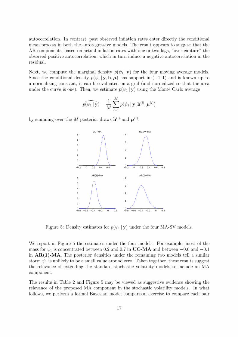
Next, we compute the marginal density p(ψ1 |y) for the four moving average models.Since the conditional density p(ψ1 |y,h,µ) has support in (−1, 1) and is known up toa normalizing constant, it can be evaluated on a grid (and normalized so that the areaunder the curve is one). Then, we estimate p(ψ1 |y) using the Monte Carlo average

p(ψ1 |y) =1

M

M∑

i=1

p(ψ1 |y,h(i),µ(i))

by summing over the M posterior draws h(i) and µ(i).

−0.2 0 0.2 0.4 0.60

1

2

3

4

5

6UC−MA

−0.2 0 0.2 0.4 0.6 0.80

1

2

3

4UCSV−MA

−0.8 −0.6 −0.4 −0.2 0 0.20

1

2

3

4AR(2)−MA

−0.8 −0.6 −0.4 −0.2 0 0.20

1

2

3

4

5

6AR(1)−MA

Figure 5: Density estimates for p(ψ1 |y) under the four MA-SV models.

We report in Figure 5 the estimates under the four models. For example, most of themass for ψ1 is concentrated between 0.2 and 0.7 in UC-MA and between −0.6 and −0.1in AR(1)-MA. The posterior densities under the remaining two models tell a similarstory: ψ1 is unlikely to be a small value around zero. Taken together, these results suggestthe relevance of extending the standard stochastic volatility models to include an MAcomponent.

The results in Table 2 and Figure 5 may be viewed as suggestive evidence showing therelevance of the proposed MA component in the stochastic volatility models. In whatfollows, we perform a formal Bayesian model comparison exercise to compare each pair

17

of stochastic volatility models (i.e., with and without the MA component) using Bayesfactors (see, e.g., Koop, 2003, p. 3–4). Since we are comparing nested models, the Bayesfactor in favor of the model that has the MA component against the standard variant canbe computed using the Savage-Dickey density ratio (Verdinelli and Wasserman, 1995):

BF =p(ψ1 = 0)

p(ψ1 = 0 |y).

In other words, we simply need to evaluate the marginal prior and posterior densities forψ1 at 0. The ratio of the two values then gives the relevant Bayes factor. The numeratordensity is a univariate truncated normal, and can be easily evaluated. The denominator

density is not of standard form, but we can estimate it using p(ψ1 = 0 |y).

The results are reported in Table 3. For each of the four pairwise comparisons—UC-MAagainst UC, UCSV-MA against UCSV, AR(1)-MA against AR(1), and AR(2)-MA against AR(2)—there is strong to overwhelming evidence that the data prefer thevariant with the MA component. Remember that each pair of the models only differs inan extra parameter ψ1, and the stochastic volatility models are standard in the literature.Given the context, these full sample estimation results present strong evidence in favorof the proposed models against their counterparts without the MA component. Not onlydo the former models fit the data better, they also give more sensible underlying inflationestimates. In the next section, we present forecasting results that show the proposedmodels also provide more accurate point and density forecasts.

Table 3: Bayes factors in favor of the proposed models against the standard variants withonly stochastic volatility.

UC-MA UCSV-MA AR(1)-MA AR(2)-MA1.78× 107 5.41 1.75× 103 6.47

So far we have fixed q, the number of MA terms, to be one. We now briefly discuss thechoice of q in general. One natural way to proceed is to view the problem as a modelcomparison exercise. For example, to compare models with q and q + 1 MA terms, wesimply need to compute the relevant Bayes factor. Specifically, since we have nestedmodels, the Bayes factor in favor of the MA(q) model can be obtained using the Savage-Dickey density ratio p(ψq+1 = 0 |y)/p(ψq+1 = 0), which can be estimated using themethod described previously.

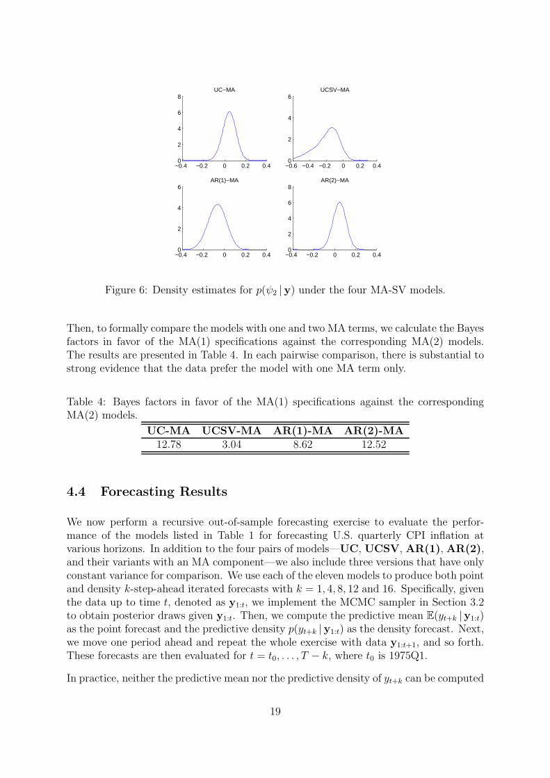
As an illustration, we investigate if there is empirical support for models with two MAterms. First, we plot the density estimates for p(ψ2 |y) under the four MA-SV modelsin Figure 6. It is clear that for each of the density, there is substantial mass around 0,indicating that ψ2 is quite likely to be a small value. This can be viewed as evidencesupporting models with only one MA term.

18

−0.4 −0.2 0 0.2 0.40

2

4

6

8UC−MA

−0.4 −0.2 0 0.2 0.40

2

4

6AR(1)−MA

−0.4 −0.2 0 0.2 0.40

2

4

6

8AR(2)−MA

−0.6 −0.4 −0.2 0 0.2 0.40

2

4

6UCSV−MA

Figure 6: Density estimates for p(ψ2 |y) under the four MA-SV models.

Then, to formally compare the models with one and two MA terms, we calculate the Bayesfactors in favor of the MA(1) specifications against the corresponding MA(2) models.The results are presented in Table 4. In each pairwise comparison, there is substantial tostrong evidence that the data prefer the model with one MA term only.

Table 4: Bayes factors in favor of the MA(1) specifications against the correspondingMA(2) models.

UC-MA UCSV-MA AR(1)-MA AR(2)-MA12.78 3.04 8.62 12.52

4.4 Forecasting Results

We now perform a recursive out-of-sample forecasting exercise to evaluate the perfor-mance of the models listed in Table 1 for forecasting U.S. quarterly CPI inflation atvarious horizons. In addition to the four pairs of models—UC, UCSV, AR(1), AR(2),and their variants with an MA component—we also include three versions that have onlyconstant variance for comparison. We use each of the eleven models to produce both pointand density k-step-ahead iterated forecasts with k = 1, 4, 8, 12 and 16. Specifically, giventhe data up to time t, denoted as y1:t, we implement the MCMC sampler in Section 3.2to obtain posterior draws given y1:t. Then, we compute the predictive mean E(yt+k |y1:t)as the point forecast and the predictive density p(yt+k |y1:t) as the density forecast. Next,we move one period ahead and repeat the whole exercise with data y1:t+1, and so forth.These forecasts are then evaluated for t = t0, . . . , T − k, where t0 is 1975Q1.

In practice, neither the predictive mean nor the predictive density of yt+k can be computed

19

analytically. Instead, they are obtained using predictive simulation. More precisely, atevery MCMC iteration, given the model parameters and states (up to time t), we simulatefuture states from time t + 1 to t + k using the relevant transition equations. We alsosimulate future errors us ∼ N (0, ehs) or us ∼ N (0, σ2

y) for s = t + 1, . . . , t + k − 1.Given these draws, yt+k is a normal random variable as specified in (1), and one caneasily produce the point and density forecasts for yt+k. Hence, we have a pair of forecasts(point and density) at every MCMC iteration. These forecasts are then averaged over allthe posterior draws to produce estimates for E(yt+k |y1:t) and p(yt+k |y1:t). The wholeexercise is then repeated using data up to time t + 1 to produce E(yt+k+1 |y1:t+1) andp(yt+k+1 |y1:t+1), and so forth.

Let yot+k denote the observed value of yt+k that is known at time t+ k. The metric usedto evaluate the point forecasts is the root mean squared forecast error (RMSFE) definedas

RMSFE =

√∑T−k

t=t0(yot+k − E(yt+k |y1:t))2

T − k − t0 + 1.

To evaluate the density forecast p(yt+k |y1:t), one natural measure is the predictive like-lihood p(yt+k = yot+k |y1:t), i.e., the predictive density of yt+k evaluated at the observedvalue yot+k. Clearly, if the actual outcome yot+k is unlikely under the density forecast,the value of the predictive likelihood will be small, and vise versa; see, e.g., Geweke andAmisano (2011) for a more detailed discussion of the predictive likelihood and its con-nection to the marginal likelihood. We evaluate the density forecasts using the sum oflog predictive likelihoods:

T−k∑

t=t0

log p(yt+k = yot+k |y1:t).

For this metric, a larger value indicates better forecast performance.

Table 5 presents the point forecast results for the eleven models. For easy comparison,we report the ratios of RMSFEs of a given model to those of UC. Hence, values smallerthan unity indicate better forecast performance than UC. A few broad observations canbe drawn from these forecasting results. First, except for UCSV, there is clear evidencethat the proposed models perform better than the standard variants for short-horizonforecasts. For instance, in comparing one-quarter-ahead forecasts, the RMSFE for UC-MA is 92% of the value for UC. Remember that the latter is among the best forecastingmodels in the literature. Clearly, these results provide strong evidence that the additionof the MA component gives substantial benefits. Second, for medium-horizon forecasts(e.g., k > 8), each of the three pairs—UCSV and UCSV-MA, AR(1) and AR(1)-MA, AR(2) and AR(2)-MA—give almost identical RMSFEs. For UC-MA, however,it consistently gives better point forecasts compared to UC, even at four-year forecasthorizon. This might seem surprising at first glance, as the MA component only modelsshort-run dynamics. However, the results in Section 4.3, especially Figure 3, suggest oneexplanation: by including the MA component, one obtains smoother and more reasonableestimates for the underlying inflation, which in turn help produce better forecasts atlonger horizons.

20

Table 5: Relative RMSFEs for forecasting quarterly CPI inflation relative to UC.

h = 1 h = 4 h = 8 h = 12 h = 16UC 1.00 1.00 1.00 1.00 1.00UC-MA 0.92 0.98 0.94 0.92 0.93UCSV 0.94 1.00 1.06 1.08 1.08UCSV-MA 0.94 1.00 1.06 1.09 1.07AR(1) 0.96 0.95 0.96 0.96 0.96AR(1)-MA 0.93 0.95 0.97 0.97 0.96AR(2) 0.96 0.96 0.97 0.96 0.95AR(2)-MA 0.94 0.95 0.97 0.97 0.95UC-MA-NoSV 0.96 1.03 0.97 0.95 0.96AR(1)-MA-NoSV 0.94 0.99 1.00 0.99 0.99AR(2)-MA-NoSV 0.94 1.00 1.01 0.99 1.00

The results also show the importance of allowing for stochastic volatility. For example,UC-MA dominates the version without stochastic volatility—UC-MA-NoSV—at allforecast horizons. Comparing AR(1)-MA and AR(2)-MA with the correspondingvariants without stochastic volatility tells a similar story. Lastly, it is also of interestto note that UCSV performs better than UC at short-horizon forecasts but worse atlonger horizons. This is consistent with the estimation results presented in Figure 3:by including stochastic volatility in the transition for τt, the estimates for underlyinginflation under UCSV traces closely the actual inflation, which is good for short-horizonforecasts but not for longer horizons. However, by including an MA component, UC-MAoutperforms UCSV-MA at all horizons.

Table 6: Sum of log predictive likelihoods for forecasting quarterly CPI inflation relativeto UC.

k = 1 k = 4 k = 8 k = 12 k = 16UC 0.0 0.0 0.0 0.0 0.0UC-MA 6.5 6.3 15.0 20.5 20.9UCSV 0.0 -4.4 -7.7 -12.1 -16.4UCSV-MA 1.7 -2.1 -6.5 -11.2 -13.2AR(1) 1.2 2.8 5.5 6.3 8.0AR(1)-MA 6.9 8.1 10.4 11.4 12.1AR(2) 3.2 5.6 8.5 8.9 10.2AR(2)-MA 5.9 7.5 9.9 11.1 11.7UC-MA-NoSV -22.3 -16.5 -6.1 -4.5 -4.2AR(1)-MA-NoSV -18.8 -13.7 -11.2 -12.5 -9.8AR(2)-MA-NoSV -19.1 -18.9 -14.3 -14.2 -11.6

We present the results for the density forecasts in Table 6. For easy comparison, wefirst compute the sum of log predictive likelihoods of a given model, and from which we

21

subtract the corresponding value of UC. Hence, positive values indicate better forecastperformance than UC. These results indicate that the addition of the MA componentprovides substantial benefits not only for short-horizon density forecasts, but also forlonger horizons. Moreover, models which do not allow for time-varying variance per-form quite badly compared to similar models with stochastic volatility, indicating theimportant role of stochastic volatility in producing good density forecasts.

5 Concluding Remarks and Future Research

With the aim of expanding the toolkit for analyzing time series data, we have introduceda new class of models that generalizes the standard stochastic volatility specificationto include a moving average component. The addition of the MA component leads tomodels that are more robust to misspecification, which often translates into better forecastperformance in practice. A drawback of the new models is that the estimation is moredifficult, as the MA component induces serial dependence in the observations. In view ofthis, we introduce a novel algorithm that exploits the special structure of the models —that the covariance matrix for the observations is sparse, and therefore fast routines forsparse matrices can be used.

We illustrate the relevance of the new class of models with an empirical application in-volving U.S. CPI inflation. Our empirical results show that the data strongly favor thenew models over the standard variants with only SV. In a recursive forecasting exercise,there is clear evidence that the new models deliver improvements in out-of-sample fore-casts. A second finding is that by allowing for SV in the error variance and imposingstationary conditions on the conditional mean process, parsimonious ARMA models canbe competitive against more complex models such as the unobserved components models.In this paper we have only considered univariate models. For future research it wouldbe interesting to formulate multivariate versions of the proposed MA-SV models, using,e.g., factors with SV, and extend the new estimation methods to those settings.

Appendix

In this appendix we outline a posterior simulator for estimating the AR-MA model:

yt = φ0 + φ1yt−1 + · · ·+ φpyt−p + ut + ψ1ut−1 + · · ·+ ψqut−q,

ht = µh + φh(ht−1 − µh) + εht ,

with |φh| < 1, where ut ∼ N (0, eht) and εht ∼ N (0, σ2h). The transition equation for ht is

initialized with h1 ∼ N (µh, σ2h/(1− φ2

h)).

Let φ = (φ0, φ1, . . . , φp)′, and we assume independent priors for φ, ψ, φh, µh and σ2

h.The priors for ψ, φh, µh and σ2

h are given in Section 3.2. As for φ, we take the following

22

truncated multivariate normal prior

φ ∼ N (φ0,Vφ)1l(φ ∈ Aφ),

where φ0 = 0,Vφ = 5×I and Aφ is the set where the roots of the autoregressive polyno-mial associated with φ are all outside the unit circle. The posterior simulator sequentiallydraws from: (1) p(φ |y,h,ψ); (2) p(h |y,φ,ψ, µh, φh, σ2

h); (3) p(ψ, σ2h |y,φ,h, µh, φh) =

p(ψ |y,φ,h) p(σ2h |h, µh, φh); (4) p(µh |h, σ

2h, φh); and (5)p(φh |h, µh, σ2

h).

Steps 2-5 can be implemented as in the sampler given in Section 3.2, and here we focuson Step 1. To this end, we first write the observation equation in matrix form:

y = Xφ+Hψu,

where X is a T × (p + 1) matrix of intercepts and lagged observations appropriately

defined. Now let y = H−1ψ y and X = H−1

ψ X, both of which can be computed quickly asHψ is banded. Then,

(y |ψ,φ,h) ∼ N (Xφ,Sy),

where Sy = diag(eh1, . . . , ehT ). It follows that

(φ |y,h,ψ) ∼ N (φ,Dφ)1l(φ ∈ Aφ),

where Dφ = (X′S−1yX+V−1

φ )−1 and φ = DφX′S−1

yy. A draw from the truncated density

can then be obtained via the acceptance-rejection sampling (e.g., Kroese, Taimre, and

Botev, 2011, chapter 3) with proposal density N (φ,Dφ). This step is efficient when φ islow-dimensional, as is often the case.

References

C. Andrieu and J. Thoms. A tutorial on adaptive MCMC. Statistics and Computing, 18(4):343–373, 2008.

G. Athanasopoulos and F. Vahid. VARMA versus VAR for macroeconomic forecasting.Journal of Business and Economic Statistics, 26(2):237–252, 2008.

T. Bollerslev. Generalized autoregressive conditional heteroskedasticity. Journal of

Econometrics, 31(3):307–327, 1986.

J. C. C. Chan and I. Jeliazkov. Efficient simulation and integrated likelihood estimationin state space models. International Journal of Mathematical Modelling and Numerical

Optimisation, 1:101–120, 2009.

J. C. C. Chan, G. Koop, R. Leon-Gonzalez, and R. Strachan. Time varying dimensionmodels. Journal of Business and Economic Statistics, 30:358–367, 2012a.

J. C. C. Chan, G. Koop, and S. M. Potter. A new model of trend inflation. Journal of

Business and Economic Statistics, 31:94–106, 2012b.

23

S. Chib and E. Greenberg. Bayes inference in regression models with ARMA(p, q) errors.Journal of Econometrics, 64(12):183 – 206, 1994.

S. Chib, F. Nardari, and N. Shephard. Markov chain Monte Carlo methods for stochasticvolatility models. Journal of Econometrics, 108(2):281–316, 2002.

S. Chib, F. Nardari, and N. Shephard. Analysis of high dimensional multivariate stochas-tic volatility models. Journal of Econometrics, 134(2):341371, 2006.

T. E. Clark and T. Doh. A Bayesian evaluation of alternative models of trend inflation.Working paper, Federal Reserve Bank of Cleveland, 2011.

T. Cogley and T. J. Sargent. Drifts and volatilities: monetary policies and outcomes inthe post WWII US. Review of Economic Dynamics, 8(2):262 – 302, 2005.

T. Cogley and A. Sbordone. Trend inflation, indexation, and inflation persistence in thenew keynesian phillips curve. American Economic Review, 98:2101–2126, 2008.

T. Cogley, G. Primiceri, and T. Sargent. Inflation-gap persistence in the U.S. American

Economic Journal: Macroeconomics, 2:43–69, 2010.

L. Fahrmeir and H. Kaufmann. On kalman filtering, posterior mode estimation and Fisherscoring in dynamic exponential family regression. Metrika, 38(1):37–60, 1991.

J. Geweke and G. Amisano. Hierarchical Markov normal mixture models with applicationsto financial asset returns. Journal of Applied Econometrics, 26:1–29, 2011.

G. H. Golub and C. F. van Loan. Matrix computations. Johns Hopkins University Press,Baltimore, 1983.

A. C. Harvey. Trends and cycles in macroeconomic time series. Journal of Business andEconomic Statistics, 3(3):216–227, 1985.

E. Jacquier, N. G. Polson, and P. E. Rossi. Bayesian analysis of stochastic volatilitymodels with fat-tails and correlated errors. Journal of Econometrics, 122(1):185212,2004.

M. J. Jensen and J. M. Maheu. Bayesian semiparametric stochastic volatility modeling.Journal of Econometrics, 157(2):306–316, 2010.

S. Kim, N. Shepherd, and S. Chib. Stochastic volatility: Likelihood inference and com-parison with ARCH models. Review of Economic Studies, 65(3):361–393, 1998.

G. Koop. Bayesian Econometrics. Wiley & Sons, New York, 2003.

G. Koop and D. Korobilis. Bayesian multivariate time series methods for empiricalmacroeconomics. Foundations and Trends in Econometrics, 3(4):267–358, 2010.

G. Koop and D. Korobilis. Forecasting inflation using dynamic model averaging. Inter-

national Economic Review, 2012. Forthcoming.

24

G. Koop and S. M. Potter. Estimation and forecasting in models with multiple breaks.Review of Economic Studies, 74:763–789, 2007.

D. Korobilis. VAR forecasting using Bayesian variable selection. Journal of Applied

Econometrics, 2012. Forthcoming.

D. P. Kroese, T. Taimre, and Z. I. Botev. Handbook of Monte Carlo Methods. John Wiley& Sons, New York, 2011.

W. J. McCausland, S. Miller, and D. Pelletier. Simulation smoothing for state-space mod-els: A computational efficiency analysis. Computational Statistics and Data Analysis,55:199–212, 2011.

J. Nakajima and Y. Omori. Stochastic volatility model with leverage and asymmetricallyheavy-tailed error using GH skew Student’s t-distribution. Computational Statistics &

Data Analysis, 2012. Forthcoming.

T. Nakatsuma. Bayesian analysis of ARMA-GARCH models: A Markov chain samplingapproach. Journal of Econometrics, 95(1):57–69, 2000.

Y. Omori, S. Chib, N. Shephard, and J. Nakajima. Stochastic volatility with leverage:Fast and efficient likelihood inference. Journal of Econometrics, 140(2):425449, 2007.

G. E. Primiceri. Time varying structural vector autoregressions and monetary policy.Review of Economic Studies, 72(3):821–852, 2005.

H. Rue, S. Martino, and N. Chopin. Approximate Bayesian inference for latent Gaussianmodels by using integrated nested Laplace. Journal of the Royal Statistical Society

Series B, 71:319–392, 2009.

R. Ruiz-Cardenas, E. Krainski, and H. Rue. Direct fitting of dynamic models usingintegrated nested laplace approximations—INLA. Computational Statistics and Data

Analysis, 56(6):1808–1828, 2012.

J. H. Stock and M. W. Watson. Why has U.S. inflation become harder to forecast?Journal of Money Credit and Banking, 39:3–33, 2007.

J. H. Stock and M. W. Watson. Modeling inflation after the crisis. Working Paper 16488,National Bureau of Economic Research, October 2010.

S. J. Taylor. Modelling stochastic volatility. Mathematical Finance, 4:183–204, 1994.

I. Verdinelli and L. Wasserman. Computing Bayes factors using a generalization of theSavage-Dickey density ratio. Journal of the American Statistical Association, 90(430):614–618, 1995.

25