
Movin' Out: Crime and HUD's HOPE VI Initiative - … Cahill Samantha Lowry P. Mitchell Downey Movin...
95
Meagan Cahill Samantha Lowry P. Mitchell Downey Movin’ Out: Crime displacement and HUD’s HOPE VI Initiative RESEARCH REPORT August 2011 URBAN INSTITUTE Justice Policy Center
Transcript of Movin' Out: Crime and HUD's HOPE VI Initiative - … Cahill Samantha Lowry P. Mitchell Downey Movin...

Meagan CahillSamantha Lowry
P. Mitchell Downey
Movin’ Out:Crime displacement and
HUD’s HOPE VI Initiative
RESEARCH REPORTAugust 2011
URBAN INSTITUTEJustice Policy Center


URBAN INSTITUTE Justice Policy Center
2100 M Street NW Washington, DC 20037www.urban.org
© 2011 Urban Institute
This report was prepared under cooperative agreement 2007-IJ-CX-0020 with the National Institute of Justice, U.S. Department of Justice. Opinions expressed in this document are those of the authors, and do not necessarily represent the official position or policies of the U.S. Department of Justice, the Urban Institute, its trustees, or its funders.


Acknowledgements
This study on crime displacement from public housing was sponsored by the NationalInstitute of Justice (NIJ), U.S. Department of Justice. The author is grateful to Ronald E.Wilson from NIJ for his guidance on this research. Others deserving acknowledgement arethe staff of the Housing Authority of Milwaukee, who acted as kind hosts and excellentresources of information both during and after a visit to gather information on HousingOpportunities for People Everywhere (HOPE VI) in that city. The staff of the District ofColumbia Housing Authority were also extremely helpful in providing information onHOPE VI sites under redevelopment in Washington, D.C. The help from the staff of thosetwo housing authorities was greatly appreciated.
We would also like to thank the Milwaukee Police Department and the MetropolitanPolice Department (Washington, D.C.) for allowing the use of their crime incident data forthis research.
The author would also like to acknowledge the contributions of a colleague at the UrbanInstitute: Elizabeth Davies, who helped gather relevant information and documents andwho was willing to travel to Milwaukee in March to assist with the project.
i

Executive Summary
The purpose of this project was to conduct an evaluation of the impact on crime of theclosing, renovation, and subsequent reopening of selected public housing developmentsunder the U.S. Department of Housing and Urban Development (HUD)’s HOPE VI initiative.No studies have specifically considered the effects of redevelopment of public housingunder the HOPE VI initiative on the spatial distribution of crime. The current research aimedto remedy that deficiency through an examination of crime displacement and potentialdiffusion of benefits in and around three public housing developments. The developmentswere selected from a candidate set of six HOPE VI sites in Milwaukee, Wis., and Washington,D.C., all of which were in the process of being redeveloped with HOPE VI funds during thestudy period.
Displacement refers to changes in crime patterns that occur because offenders adapttheir behavior to changes in opportunities for offending. In the context of the proposedwork, opportunity changes are the result of large-scale public housing redevelopment.Anecdotal evidence suggests that, when HOPE VI developments are demolished and con-struction begins on new housing, residents are typically moved to other public housingsites in the same city. Our assumption was that crime would move with those residentsto the new public housing locations, or to other nearby areas offering similar criminalopportunities.
Three central research questions thus guide this report:
1. Does the closing of a large high-poverty public housing development under HOPE VIinfluence patterns of crime in and around that development, and if so, how?
2. Does crime displacement or diffusion of benefits result during the time that thedevelopment is closed for rebuilding, and does crime return to previous levels whenthe development reopens?
3. Do different methodologies for examining crime displacement and diffusion of ben-efits from public housing developments yield similar results, and which is mostappropriate for studying displacement in this context?
The work entailed a statistical analysis of potential displacement or diffusion of crimefrom three selected sites, after the redevelopment timeline of each site was established.Three methods were employed: a point pattern analysis, a Weighted Displacement Quotient(WDQ), and time series analysis. The methods were compared following their applicationin each site. The results indicate that displacement of crime did not appear to be a sig-nificant problem during or following redevelopment under the HOPE VI program in thesethree sites. Instead, a diffusion of benefits was observed to some extent in each site.
We found a clear indication in all three sites that crime dropped at some point dur-ing redevelopment and that redevelopment affected crime in surrounding areas in some
ii

way—usually by decreasing it. The effects in the buffers (the areas searched for displace-ment or diffusion of benefits) varied, but for the most part, we observed a diffusion ofbenefits from the target sites outward. Additional investigation into subtypes of crimewould help to bring more specificity to the results (e.g., whether any crime preventionmethods implemented during redevelopment should target specific types of crimes thatare more vulnerable to displacement). In addition, in no site did we find any return topre-intervention crime levels following the intervention period in either the target site itselfor in the buffer areas. This indicates that the positive effects—the drops in crime—lastedat least as long as the study period, which was generally one to two years beyond the endof the intervention period.
The project also aimed to compare different methods for studying displacement. Thepoint pattern analysis had limited use in the present context, but we concluded that itwould have more utility if a specific crime such as homicide, robbery, or burglary, werestudied as opposed to studying a class of crimes such as personal or property crimes. Themethod is also quite involved, but efficiencies are gained once analyses are set up for onecontext, making it easier to apply the method in additional contexts (e.g., for additionaltime period comparisons, different areas/site boundaries, or types of crime).
While it cannot replace more rigorous statistical analyses and testing, the typical con-straints felt by most practitioners on time and resources make the WDQ best suited for theircontext. The WDQ is intuitive, easy to calculate, and does not require a long series of data.It is appropriate for use in exploring the possible effects of an intervention to determinewhether more sophisticated analyses are worthwhile. While there are drawbacks to theuse of the WDQ—it is only descriptive, it can only indicate relative (not absolute) effectsizes, and it is dependent on the parameters selected (time periods and displacement areasselected)—it is nonetheless a useful intermediate tool in the study of displacement.
Where skilled statisticians are available and a quantification of the changes in crimelevels is desired, the time series analyses methods presented here produce more rig-orous results. Our results also demonstrated the desirability of the structural VectorAutoregression (VAR) over the traditional time series method typically used in displacementresearch—single series Autoregressive Integrated Moving Average (ARIMA) modeling. TheVAR was preferable based on the simultaneous modeling of the three study areas, as op-posed to modeling each area individually.
Finally, to the extent that the three HOPE VI sites in two cities are representative of otheractual and possible HOPE VI sites, the results are applicable to other public housing sitesundergoing this type of large-scale redevelopment, especially given the comparabilityof results we found across sites and methods. The consistency with which we foundevidence of diffusion from the sites is an indication that redevelopment under HOPE VIdoes indeed lead to diffusion of crime reduction, whether via changes directly attributableto HOPE VI in the target area or indirectly by encouraging additional investment in thelarger neighborhood of the HOPE VI site, leading to additional redevelopment efforts inareas surrounding the HOPE VI site itself.
Based on our findings, we expect that housing authorities that undertake such large-scale public housing redevelopment efforts as are common under HOPE VI will likely seea diffusion of benefits to nearby areas, and those nearby areas may experience reductionsin crime levels similar to that experienced in the redevelopment site itself. Localitiesconsidering large-scale redevelopment, either under the HOPE VI program or followinga similar process, might look at specific crimes that may be displaced, such as personalcrimes (as was the case in Milwaukee) and enact policies that serve to prevent displacement
iii

specifically of those crimes from occurring.Studying displacement from public housing is an important undertaking, and the
possibility of displacement should be considered by housing authorities either alreadyundertaking such efforts or considering whether to start large-scale redevelopment. Whilethis research showed that diffusion of benefits is likely from redeveloped public housing,more work of this type—exploring different options for target area boundaries, interventionperiods, and displacement areas—can provide more evidence of the best approaches to thistype of effort and inform housing authorities of the most efficient ways to include studiesof displacement and diffusion in their redevelopment efforts. Additional research in thisvein that confirms the results here would add to the case presented by this research for thepositive effects of HOPE VI on target sites and on surrounding neighborhoods.
iv

Contents
Executive Summary ii
Contents v
List of Tables vii
List of Figures viii
List of Acronyms ix
1 Introduction 1
2 Background 42.1 HUD’s HOPE VI Program . . . . . . . . . . . . . . . . . . . . . . . . . . . . . 42.2 Crime and Public Housing . . . . . . . . . . . . . . . . . . . . . . . . . . . . . 42.3 Displacement . . . . . . . . . . . . . . . . . . . . . . . . . . . . . . . . . . . . 7
2.3.1 Spatial Displacement . . . . . . . . . . . . . . . . . . . . . . . . . . . . 82.3.2 Previous Research on Displacement . . . . . . . . . . . . . . . . . . . 9
2.4 Conclusion . . . . . . . . . . . . . . . . . . . . . . . . . . . . . . . . . . . . . . 11
3 Data and Methodology 123.1 Data . . . . . . . . . . . . . . . . . . . . . . . . . . . . . . . . . . . . . . . . . . 12
3.1.1 Qualitative Data . . . . . . . . . . . . . . . . . . . . . . . . . . . . . . 123.1.2 Police data . . . . . . . . . . . . . . . . . . . . . . . . . . . . . . . . . . 13
3.2 Methods . . . . . . . . . . . . . . . . . . . . . . . . . . . . . . . . . . . . . . . 143.2.1 Identification of Boundaries and Time Periods . . . . . . . . . . . . . 143.2.2 Analytic Methods . . . . . . . . . . . . . . . . . . . . . . . . . . . . . . 17
4 Research Sites 234.1 Milwaukee, Wisconsin . . . . . . . . . . . . . . . . . . . . . . . . . . . . . . . 234.2 Washington, D.C. . . . . . . . . . . . . . . . . . . . . . . . . . . . . . . . . . . 29
4.2.1 Capitol Gateway . . . . . . . . . . . . . . . . . . . . . . . . . . . . . . 304.2.2 Capper/Carrollsburg . . . . . . . . . . . . . . . . . . . . . . . . . . . . 33
5 Results: Milwaukee 355.1 Point Pattern Analysis . . . . . . . . . . . . . . . . . . . . . . . . . . . . . . . 385.2 WDQ . . . . . . . . . . . . . . . . . . . . . . . . . . . . . . . . . . . . . . . . . 395.3 Time Series Analysis . . . . . . . . . . . . . . . . . . . . . . . . . . . . . . . . 415.4 Conclusion . . . . . . . . . . . . . . . . . . . . . . . . . . . . . . . . . . . . . . 45
v

6 Results: Washington, D.C. 466.1 Capitol Gateway . . . . . . . . . . . . . . . . . . . . . . . . . . . . . . . . . . 46
6.1.1 Point Pattern Analysis . . . . . . . . . . . . . . . . . . . . . . . . . . . 496.1.2 Weighted Displacement Quotient . . . . . . . . . . . . . . . . . . . . . 506.1.3 Time Series Analysis . . . . . . . . . . . . . . . . . . . . . . . . . . . . 526.1.4 Conclusion . . . . . . . . . . . . . . . . . . . . . . . . . . . . . . . . . 55
6.2 Capper/Carrollsburg . . . . . . . . . . . . . . . . . . . . . . . . . . . . . . . . 566.2.1 Point Pattern Analysis . . . . . . . . . . . . . . . . . . . . . . . . . . . 596.2.2 Weighted Displacement Quotient . . . . . . . . . . . . . . . . . . . . . 606.2.3 Time Series Analysis . . . . . . . . . . . . . . . . . . . . . . . . . . . . 616.2.4 Conclusion . . . . . . . . . . . . . . . . . . . . . . . . . . . . . . . . . 64
7 Discussion and Conclusions 667.1 Results by Site . . . . . . . . . . . . . . . . . . . . . . . . . . . . . . . . . . . . 66
7.1.1 Milwaukee . . . . . . . . . . . . . . . . . . . . . . . . . . . . . . . . . . 667.1.2 Capitol Gateway . . . . . . . . . . . . . . . . . . . . . . . . . . . . . . 687.1.3 Capper/Carrollsburg . . . . . . . . . . . . . . . . . . . . . . . . . . . . 697.1.4 Summary of Results . . . . . . . . . . . . . . . . . . . . . . . . . . . . 707.1.5 Challenges . . . . . . . . . . . . . . . . . . . . . . . . . . . . . . . . . . 71
7.2 Method Comparison . . . . . . . . . . . . . . . . . . . . . . . . . . . . . . . . 717.3 Conclusion . . . . . . . . . . . . . . . . . . . . . . . . . . . . . . . . . . . . . . 74
Bibliography 76
vi

List of Tables
4.1 Milwaukee Socioeconomic Indicators . . . . . . . . . . . . . . . . . . . . . . 274.2 Washington, D.C., Socioeconomic Indicators . . . . . . . . . . . . . . . . . . 33
5.1 Reported Crimes in Study Area for Selected Years, Milwaukee . . . . . . . . 395.2 Mean Correlation Coefficients for All Year Combinations, Milwaukee . . . . 395.3 Weighted Displacement Quotient Results, Milwaukee . . . . . . . . . . . . . 405.4 Impact of Redevelopment of Highland Park, Cherry Court, and Scattered
Sites: Results of ARIMA Model for All Crime . . . . . . . . . . . . . . . . . . 425.5 Impact of Redevelopment of Highland Park, Cherry Court, and Scattered
Sites: Results of Structural VAR Models for All Crime . . . . . . . . . . . . . 44
6.1 Reported Crimes in Study Area for Selected Years, Capitol Gateway . . . . . 506.2 Mean Correlation Coefficients for All Year Combinations, Capitol Gateway 506.3 Weighted Displacement Quotient Results, Capitol Gateway . . . . . . . . . . 516.4 Impact of Redevelopment on Capitol Gateway and Barry Farms, Washing-
ton, D.C.: Results of ARIMA Model for All Crime . . . . . . . . . . . . . . . 546.5 Impact of Redevelopment of Capitol Gateway, Washington, D.C.: Results of
Structural VAR Model for All Crime . . . . . . . . . . . . . . . . . . . . . . . 546.6 Reported Crimes in Study Area for Selected Years, Capper/Carrollsburg . . 606.7 Mean Correlation Coefficients for All Year Combinations, Capper/Carrollsburg 606.8 Weighted Displacement Quotient Results, Capper/Carrollsburg . . . . . . . 616.9 Impact of Redevelopment on Capper/Carrollsburg and Syphax/Greenleaf,
Washington, D.C.: Results of ARIMA Model for All Crime . . . . . . . . . . 636.10 Impact of Redevelopment of Capper/Carrollsburg, Washington, D.C.: Re-
sults of Structural VAR Model for All Crime . . . . . . . . . . . . . . . . . . . 64
7.1 Summary of Weighted Displacement Quotient (WDQ) Results Across All Sites 67
vii

List of Figures
4.1 Redevelopment Timelines for All Five Sites Studied . . . . . . . . . . . . . . 264.2 Milwaukee Redevelopment and Comparison Sites . . . . . . . . . . . . . . . 284.3 Washington, D.C. Redevelopment and Comparison Sites . . . . . . . . . . . 31
5.1 Redevelopment Timeline, Milwaukee . . . . . . . . . . . . . . . . . . . . . . 365.2 Density of Crime Over Time, Milwaukee . . . . . . . . . . . . . . . . . . . . 375.3 Monthly difference in crime between target and comparison areas and aver-
age month-to-month change for each time period, Milwaukee . . . . . . . . 43
6.1 Redevelopment Timeline, Capitol Gateway, Washington, D.C. . . . . . . . . 476.2 Density of Crime Over Time, Capitol Gateway . . . . . . . . . . . . . . . . . 486.3 Redevelopment Timeline, Capper/Carrollsburg, Washington, D.C. . . . . . . 576.4 Density of Crime Over Time, Capper/Carrollsburg . . . . . . . . . . . . . . . 58
viii

List of Acronyms
ACF Autocorrelation Function
ARIMA Autoregressive Integrated Moving Average
CSS Community and Supportive Services
CNU Congress for the New Urbanism
CPTED Crime Prevention Through Environmental Design
DCHA District of Columbia Housing Authority
GREAT Gang Resistance Education and Training
HACM Housing Authority of the City of Milwaukee
HOPE VI Housing Opportunities for People Everywhere
HUD U.S. Department of Housing and Urban Development
MTO Moving to Opportunity
NIBRS National Incident Based Reporting System
NIJ National Institute of Justice
PACF Partial Autocorrelation Function
PSN Project Safe Neighborhoods
UCR Uniform Crime Report
UI The Urban Institute
VAR Vector Autoregression
WDQ Weighted Displacement Quotient
ix

Chapter 1
Introduction
The purpose of this project was to conduct an evaluation of the impact on crime of the clos-ing, renovation, and subsequent reopening of selected public housing developments underthe U.S. Department of Housing and Urban Development (HUD)’s Housing Opportunitiesfor People Everywhere (HOPE VI) initiative. No studies have specifically considered the ef-fects on crime of redevelopment of public housing under the HOPE VI initiative. The currentresearch aimed to remedy that deficiency through an examination of crime displacementand potential diffusion of benefits in and around five public housing developments. Thedevelopments were selected from a candidate set of six HOPE VI sites in Milwaukee, Wis.,and Washington, D.C., all of which were in the process of being redeveloped with HOPE VIfunds at the start of the research. Redevelopment of the Milwaukee sites under study tookplace from 2003–2009. Redevelopment of the East Capitol (now Capitol Gateway) site inWashington, D.C., started in 2001 and continued through 2010, the end of the research pe-riod. Redevelopment of the Arthur Capper/Carrollsburg site in Washington, D.C., startedin 2000 and also continued through 2010, the end of the research period.
Displacement refers to changes in crime patterns that occur because offenders adapttheir behavior to changes in opportunities for offending. In the context of the proposedwork, opportunity changes are the result of large-scale public housing redevelopment.The investigation of crime displacement from public housing redevelopment sites natu-rally leads to consideration of two different modes of spatial displacement. In the firstinstance, displacement can occur when public housing residents move (or are moved) tonew locations and crime moves with those individuals to their new residences. Crimedisplaced in this manner would be particularly expected in the case where large numbersof residents are moved en masse to a new location. A second mode of spatial displace-ment from public housing redevelopment sites occurs when crime itself moves out of theredevelopment site to nearby locations. In this case, the perpetrators of crime (e.g., drugdealers) might attempt to maintain their criminal activities in the same general area, butare forced out of the redevelopment site itself. Or, the criminal opportunity structure inthe redevelopment site is changed with redevelopment but nearby areas still offer criminalopportunities and thus absorb the crime that would have otherwise been occurring in theredevelopment site itself.
At the outset of this research, our assumption was that crime would move via eitheror both modes of displacement: with relocated residents to their new neighborhoods, orto other nearby areas offering similar criminal opportunities. As part of previous researchefforts undertaken by The Urban Institute (UI), police officials in other cities have reported
1

CHAPTER 1. INTRODUCTION
to UI that closing public housing under HOPE VI resulted in crime migration to other publichousing developments in the city or county.
Because of limitations in the data that the research team was able to collect for this study,the ability to explicitly study both of these different modes of spatial displacement was lim-ited to a certain degree. In neither Milwaukee nor Washington, D.C., were we able to obtaininformation on the locations of individual residents during and after the redevelopmentprocess. Therefore, we did not have information on whether any specific neighborhoodsreceived large numbers of displaced residents from the HOPE VI sites under study, nor werewe able to assess whether those residents moving in after redevelopment were the sameresidents who moved out prior to redevelopment. These limitations were tempered some-what, especially in Milwaukee, by one important factor: the housing authority there madea significant effort to keep residents within the redevelopment neighborhood and movedresidents around among available units as construction took place elsewhere within thesite. Therefore, while we did not have information on Milwaukee residents’ new addresses,we had good reason to believe that many, if not most, remained on site, and were thereforeable to test for both types of spatial displacement together.
In Washington, D.C., we learned from interviews with housing authority staff thatresidents were moved to any available public housing unit or given Section 8 vouchers.Those interviewed did not feel that critical masses of residents had all moved to the sameareas but rather that residents were scattered to various locations throughout the city.The lack of data on residents and the scattering of residents throughout the city madetesting the first type of spatial displacement—where crime moves with residents to theirnew neighborhoods—both impossible and, arguably, irrelevant. The second mode ofdisplacement, however, was fully testable in both Milwaukee and Washington, D.C.
Three central research questions that recognize these limitations thus guide this report:
1. Does the closing of a large high-poverty public housing development, under HOPE VIinfluence patterns of crime in and around that development and if so, how?
2. Does crime displacement or diffusion of benefits result during the time that thedevelopment is closed for rebuilding, and does crime return to previous levels whenthe development reopens?
3. Do different methodologies for examining crime displacement and diffusion of ben-efits from public housing developments yield similar results, and which is mostappropriate for studying displacement in this context?
From these questions and consideration of the types of spatial displacement that wewere able to investigate, five main hypotheses were developed and tested in the course ofthe research:
H1: The closing of the HOPE VI redevelopment sites resulted in a reduction of crime anddrug activity in the sites themselves.
H2: The closing of the HOPE VI redevelopment sites resulted in the displacement of crimeto nearby areas.
H3: Crime will be low in the immediate areas of HOPE VI sites after their redevelopmentand reopening under the HOPE VI initiative.
2

CHAPTER 1. INTRODUCTION
H4: Crime that is displaced as a result of the redevelopment of severely distressed publichousing sites under the HOPE VI initiative will persist in the displacement areas afterthe HOPE VI development is reopened.
H5: The results obtained from the selected methodologies will be comparable, allowingUI to develop a framework of displacement methodologies that are appropriate indifferent situations.
UI’s evaluation consisted mainly of a statistical analysis of crime displacement. First, toinform the statistical analysis, UI conducted interviews with local government officials andservice providers to both gather factual information on the actual process of redevelopmentin each site and to gain insight into the perceptions of those involved in the redevelopmentas to the changes in both residents and crime levels in each site. UI then conducted animpact evaluation using three different methodologies: the conceptually simple WeightedDisplacement Quotient (WDQ) (Bowers and Johnson, 2003), a point pattern analysis pro-posed by Ratcliffe (2005), and an interrupted time series design. These methods will bedescribed more thoroughly below in Section 3. The use of these three complementarymethodologies allowed UI to make a statement as to the most appropriate method forstudying displacement within the context of each site.
This report first presents a discussion of theoretical arguments supporting and refutingthe existence of displacement, methodological issues associated with studying displace-ment, and previous research on displacement. The report then provides an overview of thesites included in this study, description of each site’s redevelopment timeline, a discussionof the methods used, and the results. Finally, the report discusses the findings, payingparticular attention to the overall picture of displacement from each study site based onthe comprehensive findings from three methods, and a discussion of the utility of eachmethodology employed in various contexts.
3

Chapter 2
Background
This chapter first provides a description of HUD’s HOPE VI program. The chapter thenprovides an overview of the theory and literature on crime and public housing and spatialdisplacement, including methodological issues associated with the study and measurementof displacement and previous work on the topic.
2.1. HUD’S HOPE VI PROGRAM
Housing Opportunities for People Everywhere (HOPE VI) is a federal funding initiative be-gun in 1992 and designed to eradicate severely distressed public housing. At its inception,HOPE VI represented a radical change in housing policy with the idea that the worst publichousing developments needed extreme changes: most HOPE VI sites are demolished andreplaced with new, redesigned housing. The program also aims to reduce the concentrationof extreme poverty that is typical in targeted public housing developments; to that end,current residents of HOPE VI redevelopment sites are given the opportunity to seek housingin other areas in the private market through a voucher system.
Revitalization under HOPE VI is achieved by addressing several aspects of public housingand concentrated poverty, including redesigning the physical features of public housing,encouraging resident self-sufficiency through comprehensive service provision; relocat-ing public housing to create mixed-income neighborhoods; and using HOPE VI funds toleverage support from other sources, including nonprofits, government agencies, and localorganizations (HUD, 2007). The goals under HOPE VI are realized differently by differentHousing Authorities receiving federal monies, with each Housing Authority allowed widelatitude in its plans for redevelopment of severely distressed public housing. A unifyingtheme of funded sites, however, is design under New Urbanism principles. These princi-ples advocate ”compact, pedestrian-friendly, and mixed-use” development, mixed-incomeresidential areas, and designs that encourage social interactions (CNU, 2001). These designprinciples mesh well with the idea of ”defensible space” as defined by Newman (1996),and discussed in detail below.
2.2. CRIME AND PUBLIC HOUSING
Two main schools of thought inform this research on crime and public housing: (1) crimeand space approaches, which include ideas from the Crime Prevention Through Environ-mental Design (CPTED) school and defensible space theory and (2) social disorganization
4

CHAPTER 2. BACKGROUND 2.2. CRIME AND PUBLIC HOUSING
theory. Both of these approaches have a common focus: the importance of informal socialcontrol, manifested in this case as the ability of residents of public housing to control crim-inal behaviors. Newman’s (1972; 1996) foundational work on defensible space suggestedthat the physical design of public housing was key in preventing crime. Likewise, Popkinand colleagues’ (2004) review of HOPE VI acknowledged the often extremely unsafe condi-tions that existed in HOPE VI sites prior to redevelopment, tying public safety issues to poorphysical design of the buildings themselves. Crime is more likely in buildings where manyindividuals share the same outside entry point and dwelling units are the only privatespace, allowing individuals to become anonymous and releasing individuals from respon-sibility for the control of common areas. Residents in high rises are also physically veryfar from the street, reducing their ability to control outside areas. Street designs likewiseaffect control of public housing environments. If large ”superblocks” of public housing arelinked to the surrounding area by very few streets and limited access points to the site areavailable, the ability to patrol and control the area is diminished.
Newman’s work also recognized the role of social factors in crime prevention, andthat work dovetails nicely with theories focused more keenly on socioeconomic contextand its role in fostering social control. Joseph and colleagues’ (2007) theoretical expositionidentified the importance of interpersonal relationships in residents’ ability to exert socialcontrol to improve safety and quality of life. Many factors influence the number andstrength of such interpersonal relationships. Family disruption—including divorce orsingle parenting—can affect the ability of adults to form local networks, thereby decreasinglocal levels of social control (Felson, 2002; Sampson and Laurtisen, 1994). Such local controlcan take the form of recognizing strangers in the area, guarding each other’s property, andproviding supervision for youths (Sampson, 1997). Single and divorced persons, however,are more likely to live in primary-individual households and to spend more time outsideof the home (a fact partially determined by sociodemographic factors like age). More timeaway from home means increased proximity to offenders and decreased guardianship ofthe home. Even if single or divorced residents are at home, the level of guardianship inthese areas tends to be lower than in households where more than one person resides.Thus, ”regardless of one’s household family composition and even proximity to offenders,living in a community with low guardianship and surveillance may increase victimizationrisk” (Sampson and Wooldredge, 1987, p. 373).
Poverty can also contribute to increased social disorganization in several ways. Highlevels of poverty can leave residents lacking any of the resources necessary to organize in theneighborhood—residents may be unable to attract or harness resources that would allowthem to make changes in the community. This lack of resources in turn can lead residentsto become disengaged in the community, weakening social ties and informal networks.Neighborhood poverty can have the effect of increasing the isolation of residents fromsocial mainstreams, furthering their inability to control, or even promoting the acceptanceof, deviant forms of behavior (Massey, 2001; Morenoff, Sampson, and Raudenbush, 2001).Finally, high population density and concentrated unemployment have also been tied todecreased levels of social control.
These perspectives have guided the investigation of public housing and crime overthe past several decades, and it is commonly recognized that the residents of the kinds ofseverely distressed public housing sites targeted by HOPE VI are disproportionately affectedby crime. Researchers using victimization surveys and police crime data have documentedboth a high fear of crime among public housing residents and high violent offending ratesin neighborhoods with public housing developments. DeFrances and Smith (1998) found
5

CHAPTER 2. BACKGROUND 2.2. CRIME AND PUBLIC HOUSING
a higher level of more serious victimization among residents, and a HUD study (2000)revealed that firearm-related victimizations among public housing residents were morethan double those for the general population.
Pyle (1976) suggested that areas with public housing tended to bring in a substantialnumber of offenders from surrounding areas, while more recent research by Fagan andDavies (2000) found that violent crime tended to be associated with public housing units.The authors, examining a variety of crime categories (rape, robbery, assault, murder, andlethal violence) in and around a public housing development in the Bronx, found that theproportion of total offenses was even greater in areas within 100 yards of the projects thanin the public housing developments themselves. They also found that the rate of crimein public housing predicted crime rates in the larger census tract for rape, robbery, andmurder, suggesting that crime diffused outward. Additionally, assault and lethal violentcrime in the census tract predicted crime within the public housing units, leading theauthors to conclude that crime also diffused inward as criminals seek out public housingareas for offending. Likewise, Dunworth and Saiger (1994) found higher rates for drugarrests and violent crime in areas with public housing compared to similar neighborhoods.This relationship between public housing and crime is supported by further evidence thatthe environment of many public housing complexes attracts drug trafficking and violence(Fosburg, Popkin, and Locke, 1996; Popkin, Levy, Harris, Comey, Cunningham, Buron,and Woodley, 2002).
Other researchers have studied the involvement of public housing residents in crimeand violence, with a number of studies focusing on adolescents living in public housing.For instance, Sullivan (1989) demonstrated that reported crime among public housingresidents tended to be more serious and often involved personal and drug crimes ascompared to reported crime among residents not living in public housing. Popkin andcolleagues (2000) studied criminal activity and youth involvement in three public housingdevelopments. The authors described the daily life for residents of high-rise developmentsas being characterized by high levels of crime, violence, and disorder. Recent research byIreland, Thornberry, and Loeber (2003) found further evidence that living in public housingwas related to participation in violence. The authors reported that both the prevalence andfrequency of self-reported violent offending was greater among public housing residentsthan those not living in public housing. They also suggested that the negative effects ofliving in these high-crime developments were reflected in the rising incidence of violentcrimes as youth enter late adolescence.
Although the studies mentioned above analyzed crime in and around public housing,few studies have focused on assessing the impact of large-scale changes to public housingenvironments. Of the few studies located, only one—an unpublished thesis—examinedchanges in crime after relocation and redevelopment (Jones, 2002). The author examinedthe impact on calls for service after the Charlotte Court housing development in Lexington,Kentucky, was demolished and roughly 600 residents were relocated. Results showed thatall crime types examined decreased around the development. To examine diffusion ofbenefits from the target area, two buffer zones were identified around the development.The first zone encompassed a half-mile radius around the Charlotte Court area, and thesecond zone encompassed a one-mile radius around the Charlotte Court area. The authorfound that crime decreased in both zones after residents were relocated, and concluded thatclosing the development resulted in a diffusion of benefits from the area of the developmentoutward. Although the study findings supported the author’s hypothesis, the study waslimited in that it neither controlled for the influence of other variables on crime, nor used a
6

CHAPTER 2. BACKGROUND 2.3. DISPLACEMENT
comparison area, making it difficult to conclude whether the findings reflect changes dueto the closing of Charlotte Court.
The HOPE VI efforts and their effects—both intended and unintended—have been fea-tured in mainstream media. In particular, a 2008 article in The Atlantic (Rosin, 2008) madea connection between residents who had been relocated from Memphis’ HOPE VI efforts tonew housing using Section 8 vouchers and increased levels of crime in those areas. Rosinargued that voucher holders clustered in new neighborhoods, forced to move whereverSection 8 housing was available. The article then suggested that the voucher holders’ pres-ence contributed to increasing crime rates in their new neighborhoods. The author did notconduct a statistical analysis of the relationship, however, and a rebuttal by housing andurban policy experts soon after the original piece’s publication served to dismantle manyof Rosin’s conjectures (Briggs and Dreier, 2008). For one, Rosin failed to explore other pos-sible explanations for the increase in crime in the voucher holders’ ”new” neighborhoods.She also overestimated the number of displaced residents in Memphis and the level ofclustering of those residents who used vouchers in new neighborhoods. In fact, only asmall percentage of households are granted vouchers and, as Briggs and Dreier’s (2008)rebuttal pointed out, prior research had shown a low level of concentration of voucherholders across the 50 largest metro areas in the United States.
Other than Rosin’s (2008) journalistic work on the topic, we know of no prior work oncrime and public housing that focused specifically on the redevelopment of public housingunder the HOPE VI initiative. Public housing is being renovated under this federal programnationwide, with the expectation that quality of life in the immediate and surroundingareas will be greatly improved. The question of the benefit of the program for communitiesspecifically in terms of crime, however, has been left largely unanswered, and this researchsought to address that question.
2.3. DISPLACEMENT
Not surprisingly, measuring displacement is complex—there are many types of displace-ment, and displacement is not easy to detect among the myriad reasons for fluctuations incrime rates. Barr and Pease’s (1992) discussion on the movement of crime even suggestedthat the term ”crime flux” was a more accurate description of moving crime patterns oftentermed ”displacement.” The criminological literature recognizes six types of displacement(Repetto, 1976; Hakim and Rengert, 1981):
1. Spatial: offenders commit crimes elsewhere;
2. Tactical: crimes are committed in a way that evades the impact of the law enforcementintervention;
3. Temporal: the same kind of crimes are committed at different times;
4. Target redirection: crimes are perpetrated against different targets;
5. Functional: perpetrators switch from one type of crime to another;
6. Perpetrator replenishment: new offenders may simply step in to fill the gap createdby the intervention.
7

CHAPTER 2. BACKGROUND 2.3. DISPLACEMENT
The range of possibilities for displacement constitutes a serious challenge to preventionand law enforcement activities, and displacement is often difficult to measure and assess.While this research recognized the complexities of possible crime displacement, this workfocused only on the spatial displacement of crime. The intent was to examine whethercriminals or potential offenders moved their activities to another location after the closingof selected HOPE VI redevelopment sites in Milwaukee, Wis., and Washington, D.C., andthe subsequent reopening of the sites.
2.3.1. Spatial Displacement
Central to any crime prevention initiative is the expectation that the initiative will preventcrime. Local partners or evaluators typically measure changes in crime within the targetarea before and after the implementation of a program or intervention to examine whethercrime was prevented. Also central to crime prevention is understanding and measuringwhether and how crime was displaced from the target area as a result of the program.The issue of how to predict possible spatial crime displacement, and test for it after anintervention, is one that has been the focus of environmental criminologists for at least thepast three decades (Brantingham and Brantingham, 1993; Cornish and Clarke, 1987; Gabor,1981, 1990; Repetto, 1976; Sherman, Gartin, and Buerger, 1990).
Criminological and sociological theories support the concept of displacement throughtwo general premises: (1) when some types of crime opportunities are reduced, othersmay increase; and (2) crime is opportunistic: potential offenders seek out opportunities forcrime (Cornish and Clarke, 1990, 1987; Felson and Clarke, 1998). Displacement of crime,then, refers to changes in crime patterns that occur because offenders adapt their behavioras a result of some change in opportunities for offending. Change in opportunities canresult from a variety of crime prevention activities—from police enforcement related activ-ities (e.g., a new crime watch program) to physical changes to the environment (e.g., theclosing of a liquor store). Recent work has shown mixed conclusions on the likelihood ofdisplacement, and has suggested that diffusion of benefits should be the focus of criminol-ogists’ attention as well (Clarke and Weisburd, 1994). In this context, the redevelopment ofHOPE VI public housing developments is seen as the ”intervention,” and while not whollycrime-prevention focused, it is expected that this type of redevelopment will reduce thelevels of crime that plague severely distressed public housing.
As mentioned in Section 1, two different modes of spatial displacement from publichousing are recognized. Displacement can occur when public housing residents move(or are moved) to new locations and crime moves with those individuals to their newresidences. One significant study, the Moving to Opportunity (MTO) experiment, exploredthe changes in criminal and delinquent behavior among public housing residents whomoved out of high-poverty areas. MTO employed a random design to assign volunteerfamilies to one of three groups: a group that received housing vouchers that could only beused in low-poverty census tracts, a group that received regular Section 8 vouchers thatcould be used anywhere, and a control group that received no housing vouchers (Kling,Ludwig, and Katz, 2004).
Participants were followed over several years to assess the impacts of the program.While the results were necessarily complex for a long-term and large experiment of thiskind, the findings on safety and delinquency are worth noting. Overall, many of thosein the experimental group (who moved to lower poverty neighborhoods) felt safer andless stressed about the crime in their neighborhood (Kingsley and Pettit, 2008). Crime
8

CHAPTER 2. BACKGROUND 2.3. DISPLACEMENT
rates were significantly lower in participants’ new neighborhoods as well, for both theexperimental and Section 8 groups.
Researchers also specifically looked at the delinquency of youths in all three groups andfound that, in the long term, females and males fared differently in their new neighborhoods(Kling et al., 2004). Females in the experimental group tended to have more successthan males, experiencing fewer lifetime arrests, especially for violent offenses. Males, onthe other hand, had fewer arrests for violent offenses but increased arrests for propertycrimes and increased levels of other delinquent behaviors. In interpreting the results,the authors suggested that popular theories for explaining the neighborhood effects onbehavior do not in fact accurately capture all of the neighborhood effects. Instead, theoriesfrom psychology that account for the different behaviors of males and females in reactionto new environments should also be considered.
The MTO findings are relevant to this work because they are tied to hypotheses aboutcrime moving with residents to new neighborhoods. The MTO research suggests that ingeneral, moving from high-poverty and high-crime public housing areas—like the sitesstudied for this research—to new neighborhoods with vouchers (even if no attempt ismade to move to a particularly low-poverty neighborhood) results in improved safetyoutcomes. On the other hand, at the individual level, residents who move exhibit differentbehaviors in their new homes; they aren’t universally more successful after the move, evenwhen moving to places that have lower poverty rates.
So, crime may move with residents who represent potential victims or offenders, es-pecially if they move to an area that already has high levels of crime. New residents toan area represent new potential victims. On the other hand, relocated residents might becommitting crimes themselves, and in their new neighborhood, they might continue tocommit crime. These residents would thereby increase the level of crime in the area of theirnew residence. Crime displaced in this manner would be particularly expected in the casewhere large numbers of residents are moved en masse to a new location, because individualoffenders or victims might not effect a large change on the overall levels of crime in an area.
A second mode of spatial displacement from public housing redevelopment sites isobserved when crime itself moves out of the redevelopment site to nearby locations. Inthis case, the perpetrators of crime (e.g., drug dealers) might attempt to maintain theircriminal activities in the same general area, but are forced out of the redevelopment siteitself (Caulkins, 1992). Or, the criminal opportunity structure in the redevelopment site ischanged with redevelopment but nearby areas still offer criminal opportunities and thusabsorb the crime that would have otherwise been occurring in the redevelopment site itself.
This work will focus mainly on the second mode of spatial displacement—crime movingto areas near the redevelopment site, instead of to displaced residents’ new neighborhoods.While the work recognizes the importance of considering the first mode of displacement(crime moving with residents), we lacked the required data to make assessment of thatmode of displacement possible.
2.3.2. Previous Research on Displacement
Prior research in this area has largely focused on displacement (usually spatial) that occursas the result of a focused police enforcement effort or police intervention. The interven-tions are typically focused on small hot spots of crime—several square blocks at most—andhave distinct periods of implementation. The prevailing view has been that the potentialfor spatial displacement is high, creating some hesitation to implement such focused in-
9

CHAPTER 2. BACKGROUND 2.3. DISPLACEMENT
terventions. The literature, however, is limited, and those studies that have considereddisplacement have shown mixed results. Essentially, there is no clear or consistent find-ing in the literature regarding the likelihood that displacement will occur or what wouldbe the expected magnitude of any displacement that might occur. In fact, Braga’s (2001)review of studies on hot spot policing paid particular attention to those studies that consid-ered displacement; the review found only one of five studies that looked for displacementconcluded that displacement had occurred.
Within the past decade, a handful of studies have cautiously reported finding displace-ment, but findings overall remain mixed. Barclay, Buckley, Brantingham, Brantingham,and Whinn-Yates (1996) studied motor vehicle theft in suburban Vancouver, Canada. Theauthors used time series analysis to study displacement subsequent to a police bike patrolprogram, and considered displacement of crime to areas noncontiguous to the target areabut well known for motor vehicle theft. They concluded that displacement did occur toone of the displacement areas they considered. Lawton, Taylor, and Luongo (2005) foundevidence of displacement of drug crimes in their study of targeted police enforcement inPhiladelphia. Using Autoregressive Integrated Moving Average (ARIMA) time series meth-ods, the authors compared changing crime levels in the selected areas. In addition to thedisplacement of drug crimes, the authors found a diffusion of benefits for violent crimes.They argue that this dichotomy makes sense: violent crimes are not generally planned andare not location-specific. Drug markets, however, tend to be geographically-focused andare highly planned. The reaction of these different types of offenders to targeted policeenforcement, then, was expected to be different.
Additional studies have found that instead of displacement, a diffusion of benefits fromthe intervention actually occurs in neighboring areas. Fritsch and colleagues’ (1999) studyof a yearlong focused police enforcement in Dallas, Texas, compared crime frequenciesin target and comparison areas using t-tests. They concluded that no displacement hadoccurred to comparison areas as a result of the police efforts. Braga and colleagues’ (1999)study of problem oriented policing in Jersey City, New Jersey, employed a randomized con-trolled experimental design to compare treatment and non-treatment areas. Using Poissonregression analysis, the authors determined that for most crimes, displacement had notoccurred, but that for property crimes in particular, a significant amount of displacementhad occurred. The authors pointed out that the level of displacement that occurred didnot negate the drops in property crime that occurred in the targeted area. In addition, forother crimes, an apparent diffusion of benefits was noted.
Green Mazerolle, Price, and Roehl (2000) studied a civil remedy program in Oakland,Calif., to compare the difference between traditional police handling of problem propertiesand an alternative civil remedy method. They considered displacement within a 500-footradius of each targeted property and found that while civil remedies appeared to reduceproblems in the area—diffusing benefits to nearby areas—traditional policing actuallycreated more problems in nearby areas, displacing problems. Smith’s (2001) study ofRichmond Va.’s Blitz to Bloom initiative, which involved a crackdown and cleanup ofa targeted area, also found a diffusion of benefits in two of three displacement areasconsidered.
Weisburd, Wycoff, Ready, Eck, Hinkle, and Gajewski (2006), also in Jersey City, NewJersey, studied displacement and diffusion from two hot spots (one prostitution, one drug)targeted for increased police interventions. Their effort included extensive social observa-tions in the target and ”catchment” areas (where the authors searched for displacementand/or diffusion of benefits), which were used to measure the effects of the intervention.
10

CHAPTER 2. BACKGROUND 2.4. CONCLUSION
The study found that benefits of the increased police efforts in the hot spots diffused tothe catchment areas. While the authors recognized the limited generalizability of a studybased on only two hot spots, the work did present a novel approach to measuring theeffects of police interventions (social observation) and they suggested that the conclusions,specifically pertaining to prostitution and drug crimes, were ”persuasive.” The authorsalso pointed out that new ideas in routine activity and rational choice theories suggestedthat diffusion of benefits should actually be expected.
Finally, Braga and Bond (2008) looked at the effects of a targeted police strategy inLowell, Massachusetts. That effort specifically targeted disorder, and the study looked atmore serious crimes to determine the effects of policing disorder on those crimes. LikeWeisburd et al. (2006), the study employed social observations to measure some of the im-pacts of the police efforts; calls for police service were used as official indicators of crime.While significant results indicated that there was no displacement, some nonsignificant re-sults suggested ”minor immediate spatial displacement of crime.” The authors cautioned,however, that displacement was hard to measure and that other positive effects of theintervention outweighed any displacement that might have occurred.
Displacement, then, has been neither extensively studied nor universally identified,and there appears to be reason to question the traditional thought assuming and expectingits existence. In addition, if the number of studies focused on displacement of crime fromtargeted police interventions has been limited, the number that have considered crimedisplacement from public housing redevelopment efforts has been nearly non-existent. Itis this gap in the literature that the present study aimed to fill.
2.4. CONCLUSION
The possibility of displacement—either spatial or otherwise—has been the focus of a gooddeal of debate among researchers and practitioners, with no clear consensus resultingon the potential for displacement, the best methods for measuring the phenomenon, orappropriate prevention methods. What was clear at the start of this research was that lawenforcement agencies, housing authorities, and the neighborhoods they seek to protectwould benefit from a greater understanding of what actually does take place when publichousing is redeveloped under HOPE VI. Filling that need was the primary focus of thisresearch, and its intent was to examine whether criminals or potential offenders movedtheir activities to another location after the closing and subsequent reopening of three HOPEVI redevelopment sites.
The next chapter discusses the data collected for each site and the methods used tosearch for displacement of crime or diffusion of benefits.
11

Chapter 3
Data and Methodology
The goal of this research was to examine crime displacement from five HOPE VI sites in twocities using three different methodologies (the WDQ, point pattern analysis, and time seriesanalysis). Crime in each site was examined using official police records from the policedepartments in Milwaukee, Wis., and Washington, D.C., over a nearly 10-year period. Inaddition, a comparison group design was used whereby appropriate comparison areaswere selected for each site and also examined over the same time period. The comparisonsites were used to determine whether changes in crime levels, unrelated to HOPE VI orthe redevelopment efforts in each site, were taking place citywide. The comparison sitedesign allows researchers to more confidently attribute any observed changes in a studyor intervention site to the intervention itself. The comparison sites were also assessedusing official police records on crimes reported. In each site, police data were collected forthe period 2000–2009 for use in the study. This allowed for at least one year before anysite started redevelopment (the pre-period), and a varied number of months or years afterredevelopment, determined by the redevelopment timeline (the post-period).
This chapter outlines the specific data that were collected for each site, the definition ofsite boundaries and displacement and comparison areas, and the redevelopment timeline.The chapter also presents the three methods used to examine displacement under thisresearch study.
3.1. DATA
3.1.1. Qualitative Data
Qualitative data in the form of information about each site were collected via interviewswith staff members of Housing Authority of the City of Milwaukee (HACM) and District ofColumbia Housing Authority (DCHA). Staff members at both agencies were very helpfuland were invaluable sources of information and documents on the HOPE VI applicationsand awards, redevelopment plans, residency requirements, perceived changes in each site,and progress made to date at each site. This information was used in determining thetimelines for redevelopment in order to define pre-, during-, and post-intervention periodsfor use in the analyses.
Project staff had hoped to learn more about the residents for each site, including whereeach resident moved during the relocation period, what types of housing the residentswere moved to when relocated, and which former residents returned to occupy newlybuilt units. This information, however, was not readily available from either housing
12

CHAPTER 3. DATA AND METHODOLOGY 3.1. DATA
agency; neither agency shared data on specific residents with project staff. The informationon residents was desired in order to test for the first ”mode” of displacement, where crimemoves with residents to their new neighborhoods (see Section 1). The data on residents’new addresses after relocation would have allowed us to identify areas of possible crimedisplacement not adjacent to the sites themselves (e.g., sites to which crime might havemoved because a number of residents left a HOPE VI site and most moved to the same newlocation), following the technique of Roman and colleagues’ (2005) work in Miami.
In Milwaukee, where most residents were simply ”shuffled” around to available unitswithin the redevelopment neighborhood, this did not pose a large problem; there wasnot an obvious alternate location to which crime would be expected to be displaced. InWashington, D.C., DCHA staff reported that while they were not able to share informationon where residents were relocated, most were not moved en masse to a new location; rather,they were scattered to available units throughout the city. Some residents, however, usedhousing vouchers for nonpublic housing units, and project staff learned anecdotally thatmany residents did relocate to similar areas where Section 81 units were available. Lackinginformation on residents, however, we were unable to identify specific public housingdevelopments or neighborhoods in Washington, D.C., to which we might have expectedto see crime displaced.
Project staff had also hoped to gather information on the changing demographics ofresidents in each site to incorporate into the time series analysis models. While data werecollected on the demographics of each site prior to redevelopment and on the residencyrequirements of the new units, from this information, it was difficult to determine thedemographics of the new units. We did not have specific resident information from eitherhousing authority, Census data were outdated, and residents were continually movingin as the research progressed. We also collected the number of residents living in thedifferent sites at different points in the redevelopment process. This helped us to delineatethe different periods (e.g., pre, during, and post) for the various analyses but did notprovide enough information to warrant incorporating them into the models themselves.Therefore, we were unable to collect enough information about each site for use in statisticalmodeling methods. The qualitative data collected, however, were very useful in informingthe parameters selected for the models developed and in interpreting the results of theanalysis efforts.
3.1.2. Police data
Address-level incident data were collected for the city of Milwaukee from the MilwaukeePolice Department for the period January 2002-February 2010. Incident data includedall ”Group A” offenses as classified under the National Incident Based Reporting System(NIBRS). Addresses were geocoded using a streetfile provided by the City of Milwaukeewith a 100 percent match rate. The offenses were classified by researchers into personal(violent) and property offenses. Personal offenses included homicide, sexual offenses,assault offenses, and kidnapping. Offenses were aggregated into monthly counts, givingproject staff 110 months of data with which to conduct statistical analyses.
It should be noted that the police department in Milwaukee changed data systems inearly 2005. This shift in systems created two data issues: one was that data were missing
1The federal Section 8 program, or the Housing Choice Voucher Program, provides assistance to low-incomeindividuals and families in the form of rental subsidies for recipients. The program is administered throughHUD.
13
CHAPTER 3. DATA AND METHODOLOGY 3.2. METHODS
for the last three months of 2004. Monthly totals for those months were imputed usingdata before and after the missing months. Second, the police department reported thatdue to changes in the data system, arrest data were not available prior to 2005. Becauseredevelopment activities started prior to 2005 in Milwaukee, the existing arrest data werenot collected or used in the current research.
Address-level incident data were also collected for Washington, D.C., from the Metropoli-tan Police Department for the period January 2000 through September 2009. Incident dataincluded all Part I offenses as classified under the Uniform Crime Report (UCR) system.All data were provided with X and Y coordinates, so no geocoding was necessary. As inMilwaukee, the data were classified by researchers into personal and property offenses,following the same scheme used for the Milwaukee data. In D.C., researchers had hopedto collect arrest data in order to assess in particular the levels of drug activity occurringin the HOPE VI sites and displacement areas over the study area. The only data readilyavailable, however, were juvenile arrests. Those data were collected and processed, buttoo few arrests took place in any given site over the project period. For example, in CapitolGateway, only 26 juvenile arrests for drug charges were recorded over the nearly 10-yearstudy period. The number of arrests was therefore too low to warrant conducting anyanalyses using those data. Unfortunately, that meant that the research team was unable toevaluate changing drug crime levels in the sites.
3.2. METHODS
3.2.1. Identification of Boundaries and Time Periods
Prior to conducting any displacement analyses, the research team had to first identify theoverall timeline of redevelopment for each site under study, determine the ”intervention”point, define the site from which crime displacement might occur, and define the displace-ment areas—those sites to which crime might be displaced—and the comparison areas.Much of the previous work on crime displacement looked at targeted interventions bythe police that generally covered a small geographic area and took place over a short,well-defined time period. The HOPE VI redevelopment projects, however, were not short,nor were the sites compact areas. Identifying site boundaries, displacement areas and timeperiods, then, was not an easy task given the length of the redevelopment projects and thesize of the sites targeted for redevelopment.
Site boundaries
The process for identifying the site boundaries, the specifics of which are discussed inChapter 4, included identifying all HOPE VI redevelopment sites and all public housingsites. Several factors complicated the delineation of the target areas, or the interventionsite boundaries. HOPE VI sites are typically large and these kinds efforts often includeredevelopment of nearby areas with funds from different sources, and public housingis often clustered within neighborhoods, what results is often overlapping or vaguelydefined boundaries of public and other types of low-income housing being redevelopedusing funds from HOPE VI and other sources. The boundaries of these sites were examinedto determine which areas should be included in the ”intervention” area and what shouldnot be considered as part of the redevelopment efforts. As will be discussed later, site
14

CHAPTER 3. DATA AND METHODOLOGY 3.2. METHODS
definition was very difficult in Milwaukee but relatively straightforward in Washington,D.C.
Displacement of crime is most often studied by choosing an area to which crime willmost likely be displaced—the displacement zone—and comparing levels of crime in thatarea with the target area (area where the intervention took place). The next step in searchingfor possible displacement or diffusion of benefits, then, is to identify the area or areas towhich one can expect crime to be displaced, or to which benefits will diffuse—here, theseareas are called the ”displacement zones” or areas. The most common displacement areaused is an area surrounding the target area; this particular design is sometimes describedas a ”buffer zone.” This buffer-as-displacement zone can be concentric, reaching a setdistance in all directions from the target area, or it can be contiguous to the target area butextending only in limited directions (Hamilton-Smith, 2002). Most research thus far haslooked for immediate spatial displacement in areas contiguous to the target area (Braga,2001). The size of the zone varies in the literature as well, and Bowers and Johnson (2003)suggest that there is a ”displacement gradient” that describes displacement as decreasingwith increasing distance from the target area.
Issues with choosing a displacement zone include choosing one that is not so small asto emphasize fluctuations in the data (too small a sample of crime events) or to not capturea fair amount of displacement that could be taking place. Conversely, it is also problematicto choose a displacement zone that is too large and ”washes out” the displacement thatis taking place, masked by larger crime trends in the area. The geographic features of anarea should be taken into account in choosing a zone as well, as there may be a physicalfeature (e.g., a railroad, a river) that might prevent displacement from taking place inthat direction. Bowers and Johnson (2003) also suggest the use of multiple displacementzones, increasing in distance from the target area, for comparison purposes. Alternatively,Ratcliffe (2005) identifies no displacement zone prior to studying displacement. His flexiblemethodology allows the researcher to study changing crime patterns across an entire studyarea and identify whether the changes are the result of displacement, given the researcher’sknowledge of interventions that took place in the study area.
For this research, multiple displacement zones or areas were used. The displacementareas for both the Milwaukee and Washington, D.C., sites were drawn as concentric rings(”buffers”) around the target area. We tested two zones for displacement in each site: onering that was 1000’ from each site, and one that was 2000’ from each site. The two bufferareas were mutually exclusive; the area contained in the 2000’ buffer did not include the1000’ buffer. This allowed us to determine whether displacement or diffusion of benefitsoccurred only within areas very close to the site, or if they had a wider reach.
In the selected study sites, comparison areas were selected based on recommendationsfrom both HACM and DCHA. Comparison sites were other public housing developments thatwere similar to the redeveloped sites prior to their redevelopment. In Milwaukee, becausethe target area selected was so large, we included the area in a 3000’ buffer surroundingthe comparable public housing development as the comparison area. In Washington, D.C.,only the actual area of the comparison public housing site was used. More detail on thetarget and comparison area characteristics is provided below in Section 4.
Intervention time periods
In addition to the geographic considerations necessary in studying displacement, there aretemporal issues that need to be addressed. One is determining how soon displacement is
15

CHAPTER 3. DATA AND METHODOLOGY 3.2. METHODS
expected to occur after the start of an intervention. It is generally expected that displace-ment of crime will lag behind the introduction of an intervention to some extent. However,the lag period has not been well addressed in the literature, with prior research employinga variety of different lag periods, ranging from analyzing displacement from the start ofthe intervention (no lag period) (Smith, 2001) to analyzing displacement starting at the endof a problem-oriented policing strategy of indeterminate length (it ended when problemswere thought to be resolved) (Braga et al., 1999).
A second temporal issue related to displacement is determining the duration of dis-placement. Researchers have employed a variety of post-intervention lengths in theiranalyses, ranging from analyzing displacement only during the crackdown (no residualdisplacement expected) (Smith, 2001; Ratcliffe, 2005) to analyzing displacement up to 20months after an intervention (Bowers and Johnson, 2003). Bowers and Johnson (2003) sug-gest that small time periods of analysis are more subject to random fluctuations in crimeand confound results. They recommend that a substantially long period of time beforeand after an intervention be used to study displacement and state that the length of theintervention and expected length of residual deterrence will both play a role in determininghow long after the intervention displacement will be evidenced.
For this work, for each specific site and type of analysis, we needed to establish an”intervention” point, during and after which we could look for displacement. The WDQand point pattern analyses were tested using different pre, intervention, and post periodsfor each site. The time series analysis, however, required that we delineate non-overlappingperiods. For that analysis, we divided the timeline for each site into four major periods:
The ”pre” period: Residents are living on site and the site is more than half occupied withresidents during this period.
The ”move-out” period: Relocation of residents takes place during this period, with thenumber of residents on site diminishing with time.
The ”construction” period: Demolition of old units and buildings takes place, along withconstruction of new units, during this period.
The ”move-in/stability” period: Residents begin to move back in and the site reachesstability in terms of the percentage of units that are occupied.
These periods were not easily delineated, even with the information contained in thedetailed redevelopment timelines. One or more of these periods overlapped for all ofthe sites. For example, for some sites we identified different resident move-out periodsfrom different sections of each site. We also identified different construction projects withdifferent timelines at each site and different points of stabilization of residences on differentparts of each site. For the various analyses, however, we could not have overlappingperiods, so we chose the midpoint of the overlap period as the border between two periods(e.g., if the move-out and construction periods overlapped by six months, we chose threemonths prior to the end of the move-out period and after the start of the constructionperiod as the boundary between those two periods).
The different time periods used for each site and each analysis are specified in thediscussion of the results.
16

CHAPTER 3. DATA AND METHODOLOGY 3.2. METHODS
3.2.2. AnalyticMethods
The first step of the research was to determine whether crime dropped in the HOPE VI sitesand whether any search for displacement of crime or diffusion of benefits was appropriate.We conducted descriptive analyses of crime levels before and after redevelopment in eachsite and found that each experienced a significant decrease in crime levels and that wecould proceed with the selected methodologies, described below.
Point pattern analysis
The first technique employed in the proposed research was Ratcliffe’s (2005) point patternanalysis method. This method examines the geographic distribution of crime points in aselected study area at one time period and compares that it to the geographic distributionsof crime points in the same area in a later time period. The method, as presented byRatcliffe, does not require the identification of a specific intervention site but instead looksat patterns over a larger area. This type of point pattern analysis is designed to be flexibleand to allow exploration of varying spatial patterns over time.
The method was presented as an intermediate step in a larger assessment of potentialdisplacement; Ratcliffe suggests that the first step is identifying whether an interventionwas associated with decreased crime in the target area. The next step would be point patternanalysis to determine whether spatial patterns of crime in and around the intervention areachanged. If the patterns did change, further exploration could take place to determine whatthose changes were and what the possible cause of those changes was. This technique wasthus conducted first, after it was determined that crime did in fact decrease in the study sites.The current research, however, included additional techniques for studying displacementregardless of the results of the point pattern analysis in order to conduct a comparison ofthe results of each technique.
Ratcliffe’s method requires generation of a random point distribution in the study area.The distance from each random point in the study area to its nearest crime point is thencalculated. This is repeated, with the random points remaining the same, for two setsof crime points at different times (e.g., year 1 and year 4). The random points are thenranked in order of smallest to largest distance to nearest crime point for each different setof crime points (e.g., the distances from each random point to crime at t0 are ranked, andthe distances from each random point to crime at t1 are ranked separately). The two setsof rankings of random points are compared using Spearman rank correlation coefficients.This method is repeated multiple times using varying random point distributions (a MonteCarlo process). Once a set of Spearman rank correlation coefficients has been calculated,the distributions of coefficients can be examined for significance. If the specific significancelevel chosen was reached in that percentage of individual correlations, then the results canbe considered significant. For example, if the chosen significance level is p<0.01, and atleast 99 percent of the runs achieved that level of significance, the whole set of runs can beconsidered significant. Ratcliffe found that a set of 100 repetitions was appropriate in hisstudy. The current study followed that example and used 100 repetitions for this analysis.Varying numbers of repetitions were tested but the results remained very similar in allsites.
Another issue is the number of points used in the analysis. Ratcliffe chose 100 pointsfor his analysis of a burglary intervention in Canberra, which represented approximately5 percent of the total number of crime points in his study. He cautions, however, against
17

CHAPTER 3. DATA AND METHODOLOGY 3.2. METHODS
using so many points that the pattern becomes regular within the study site, and so few thatthe number of degrees of freedom is restrictive when calculating the correlation betweenthe two sets of distance rankings. The current research looked at spatial patterns in a muchsmaller area than an entire city, as Ratcliffe did, and tested different numbers of randompoints to compare results. Those results are presented below.
Ratcliffe also suggests a unique way to address edge effects that might occur whenusing this technique. The results might be affected when a random point is placed closer tothe boundary of the site than to a crime point in either crime series (crime at t0 and crimeat t1). In this case, it is conceivable that another crime might have occurred outside theboundary but closer to the random point than any crime at t0 or t1. To accommodate thisfact, a flexible method of excluding random points was suggested by Ratcliffe: the distanceof each random point to the border is compared with its nearest neighbor in both crimeseries. If it is closer to the border than to crime in either series, it is excluded and anotherrandom point is generated that meets the requirement. This process is continued until allrandom points are closer to crime at t0 and t1 than to the boundary. The boundary forrandom points, then, is dependent upon the spatial distribution of points in t0 and t1, andchanges if the period under analysis changes (i.e., if a comparison is made between year 1and year 2 and then between year 1 and year 4, the random point boundary is different foreach of those two analyses).
These point pattern analysis methods can actually be applied without identifying anintervention because no prior knowledge of intervention location, length, or focus is re-quired. However, knowledge of the redevelopment timeline informed the selection ofperiods for which the point pattern analysis was conducted. We compared a number ofdifferent time periods for each site in order to compare results.
The point pattern results are easily interpreted. Mean correlation coefficients that aresignificant and positive indicate no change in the spatial pattern of crimes examined.Coefficients that are significant and negative indicate a change in the spatial pattern ofcrimes, and would indicate that further investigation into the areas from and to whichdisplacement might have occurred is warranted.
After suitable random point distributions were created for the analysis in each site usingArcGIS software, the nearest neighbor distance calculations, rankings, and correlationswere computed in the statistical package R.
The following summarizes the process followed for point pattern analysis:
1. Define geographic area in which to look for point pattern changes2. Prepare two sets of crime points within study area, at t0 and t13. Determine number of random points, x, to use and number of simulations, i, to
conduct4. Address edge effects:
(a) Generate x random points within the selected study area(b) Calculate the distance of each random point to its nearest crime point at t0(c) Calculate the distance of each random point to its nearest crime point at t1(d) Discard any points that are closer to the edge of the study area than to a crime
point at t0 and t1(e) Generate replacement random points for those that did not meet the criteria
above(f) Repeat test process until all random points are closer to a crime point at t0 and
t1 than to the edge of the study area
18

CHAPTER 3. DATA AND METHODOLOGY 3.2. METHODS
5. Calculate nearest neighbor distances and rank random points:
(a) Calculate the distance from each random point to its nearest neighbor in the setof crime points at t0
(b) Rank the x random points in ascending order based on distance to nearestneighbor, save ranking at t0 (e.g., 1, 2, 3, etc.)
(c) Calculate the distance from each random point to its nearest neighbor in the setof crime points at t1
(d) Rank the x random points in ascending order based on distance to nearestneighbor, save ranking at Time 1 (e.g., 1, 2, 3, etc.)
6. Calculate the Spearman rank correlation coefficient between the two sets of rankingsfrom t0 and t1
7. Determine the test statistic (or significance level) of the correlation coefficient8. Repeat analysis process using same two sets of crime points for t0 and t1 i times9. Compile i correlation coefficients and test statistics
10. Determine significance of correlations between patterns:
(a) Select significance level(b) Determine whether appropriate percentage of correlation coefficients meet that
significance level (i.e., if chosen significance level is 95% and 95% of correlationcoefficients were significant at that level, the mean value of all i correlations isconsidered significant)
This outline of the process reveals the heavy computational requirements that can beneeded if the number of crime points or random points in any given distribution is high.The next method presented is less computationally complex but requires the delineationof discrete target, displacement, and comparison areas.
Weighted Displacement Quotient
Bowers and Johnson (2003) developed the WDQ method to assist displacement researchwhere lengthy time series pre- and post-intervention are not available. The WDQ was de-veloped to identify the possible presence of displacement or diffusion, not the absolutesize of any displacement or diffusion that might have occurred. The WDQ considers levelsof crime in three areas—target (A), displacement (B), and comparison or control (C) ar-eas. This method can be employed with point or aggregate data, with the most accurateresults obtained from point data, because point data allow the development of target, dis-placement, and comparison areas that do not follow administrative boundaries. The mostcommon method for identifying displacement zones (B) is to draw concentric rings aroundthe target area (A). That is the method that was used in the current research because of thedifficulties described above in identifying alternate locations to which displacement mighthave occurred.
The quotient has two parts: the displacement measure, which measures the change incrime in the displacement area relative to the change in crime in the control area over thesame period and is the numerator shown in Equation 3.1, and the success measure, whichmeasures the success of an intervention—the reduction (or slowed increase) of crime inthe target area relative to a comparison area, and is the denominator in Equation 3.1. Thedisplacement measure is divided by the success measure to calculate the final WDQ. Thefull formula is given as:
19

CHAPTER 3. DATA AND METHODOLOGY 3.2. METHODS
WDQ =Bt1/Ct1 − Bt0/Ct0At1/Ct1 − At0/Ct0
(3.1)
where At0 and At1 are crime levels in the target area at t0 and t1; Bt0 and Bt1 are crime levelsin the displacement area at t0 and t1; and Ct0 and Ct1 are crime levels in the comparisonarea at t0 and t1.
Prior to any search for displacement or diffusion of benefits, the researcher must firstidentify whether any positive changes in crimes levels occurred at the time of the inter-vention in the target area. The success measure (denominator) can be used to determinewhether or not such a change occurred. If the success measure is negative, then crime inthe site decreased, and the researcher can move to looking for displacement or diffusion. Ifthe success measure is positive, crime in the site actually increased over the study period,and there is no theoretical reason to look for displacement of crime.
Interpretation of WDQ results is straightforward. The value of the WDQ is often withinor near the range of -1 to 1. Larger values (positive or negative) indicate greater effects.The measure produces a positive score when there is a diffusion of benefits to the bufferarea and crime has gone down. Positive values that are less than 1 indicate diffusion, ora positive effect on crime levels in the displacement area, that is smaller than the effect ofthe intervention in the target area. Values greater than 1 indicate that the positive effectson crime levels were greater in the displacement area than in the target area. A negativescore indicates displacement of crime; values between 0 and -1 indicate that displacementdid occur, but that the negative effect in the displacement area was less than the positiveeffect of the intervention in the target area. Values less than -1 indicate that the negativeeffects (increased crime) to the displacement area were actually greater than the positiveeffects in the target area.
Although using the WDQ provides a measure of ”success” of the intervention, it isimportant to note that the measure is not a rigorous test of whether the intervention itselfsignificantly contributed to any change in crime. The WDQ can only ”suggest” success andexamine possible displacement. With careful modeling of the intervention and possible lagtimes for displacement, time series modeling provides a more appropriate test of the impactof the intervention and a stringent examination of whether displacement occurred. It is verydifficult, however, for researchers and practitioners interested in examining displacementto obtain time series crime data for a long period of time for a small neighborhood, andthe desire of policy makers to know what works immediately or soon after an interventionis implemented often precludes researchers from using an interrupted time series design.This desire for very timely results makes the WDQ valuable apart from more sophisticatedtime series analyses.
Time series analysis
Single series ARIMA models The last stage of analysis employed a time series design.To date, few studies examining displacement have used a time series design because timeseries crime data covering a long period of time are needed to conduct the analysis (forexceptions, see Roman et al., (2005) and Lawton et al., (2005)). That length of data wereavailable for the proposed study. Under this design, an outcome (crime) is observed atequally spaced intervals of time during a span in which some change in the underlyingprocess generating the outcome (i.e., HOPE VI redevelopment) is hypothesized to occur.The series of observations is examined to see if the hypothesized shift in the underlying
20

CHAPTER 3. DATA AND METHODOLOGY 3.2. METHODS
process is observable as a shift in the observations. The observations from the period oftime prior to the hypothesized change or intervention are treated as a baseline againstwhich the post-intervention observations are compared.
Conventional linear models are inappropriate for use with time series data becausethose models assume that the data being modeled are independent observations. Timeseries data, by contrast, are serially dependent, with each observation being a realizationof the same underlying process, and perhaps dependent upon the effects of earlier stagesof that process. A more appropriate analytic technique with time series data is to esti-mate an ARIMA model to the time series that yields residuals that are ”white noise” (i.e.,independently and normally distributed with a mean of zero and constant variance). Inter-vention variables are typically included; these are usually dichotomous and simply dividethe time series into different time periods that identify different stages of an intervention.Many intervention dummy variables denote only two time periods: pre-intervention andpost-intervention, but additional dummy variables can be employed to identify more thanone stage of the intervention. This research employed at least three intervention dummyvariables in each model to identify periods of resident move-out, site construction, andresident move-in. The intervention periods used in each model are discussed as part of theresults.
The generic ARMA(p,q) model thus takes the form:
Yt = α +P∑
p=1
βpyt−p +Q∑
q=1
γqεt−q + εt (3.2)
where the term∑P
p=1 βpyt−p is the AR term, βp is the AR coefficient,∑Q
q=1 γqεt−q representsthe lags of past shocks to the series, and εt represents the contemporaneous shocks orinnovations in the model.
A common threat to the external validity of an interrupted time series design is thepossibility that a change other than the hypothesized intervention affected the observedseries at the same time that the hypothesized intervention occurred. The effects of the twointerventions would then be conflated in the impact estimates. We examined a time seriesin a control area, an area unaffected by the intervention of interest (i.e., a nearby area with alarge public housing development not undergoing redevelopment), to help guard againstthis type of error. For the selected study sites, comparable public housing developmentswere selected for use as control or comparison area.
Vector Autoregressive models In order to estimate the effects of HOPE VI on the areassurrounding each site—to look for displacement or diffusion effects—we estimated a struc-tural Vector Autoregression (VAR) on three series for each site, expected to be endogenous:the target site, the 1000’ buffer, and the 2000’ buffer. The VAR model is a simultaneous equa-tions model that has been especially useful in policy analysis applications. This model wasselected based on the idea that crime in each site affects the areas immediately surroundingit, and crime in those areas affects crime in the site as well. The structural model takes intoaccount contemporaneous and lagged effects; that is, it accounts for crime happening innearby areas in the same month and in previous months.
VARs were first introduced in 1980 as a macroeconomic tool used largely for forecasting(Sims, 1980). While a standard time series model has one variable whose future values arepredicted based on its previous values alone, VAR models can include any number of linear
21

CHAPTER 3. DATA AND METHODOLOGY 3.2. METHODS
variables. Stock and Watson (2001, p. 101) describe a VAR as ”a n-equation, n-variable linearmodel in which each variable is in turn explained by its own lagged values, plus currentand past values of the remaining n-1 variables.” In developing a VAR model for each site,we used the results of the ARIMA time series analysis (e.g., the selected number of the lagsand intervention variables) and modeled the site and each of the two displacement bufferstogether. The results of the structural VAR allowed us to determine whether the changesin the site via HOPE VI directly and/or indirectly affected crime levels in the displacementareas.
A generic VAR can take the form:
AYt = β0 +P∑
p=1
βiYt−i + εt (3.3)
where there are k variables in the system and where A is a k x k matrix of contemporaneousimpact coefficients that is nondiagonal and where all values on the main diagonal are equalto 1. Yt is a k x 1 matrix and βi is a k x k matrix of autoregressive coefficients. ARIMA timeseries models were estimated using the statistical package R. VAR models were estimatedusing the statistical package Stata.
The next chapter provides an in-depth description of the sites selected for this study,including the redevelopment timeline for each site and the potential for displacement ineach site.
22

Chapter 4
Research Sites
As stated earlier, five sites were selected from a candidate set of six sites: three in Milwaukee,Wis., and two in Washington, D.C. The candidate sites in each city were those that hadbeen redeveloped using HOPE VI funds since 2000, although researchers later included anon-HOPE VI site in Milwaukee for reasons described below. The three Milwaukee siteswere analyzed together due to their close geographic proximity to each other. The sitesused for this study were selected based on the timing of the relocation of residents (e.g.,some sites sat empty for years prior to redevelopment under HOPE VI), the progress ofeach site at the start of the current research project, the number of residents residing inthe new development at the point of analysis, and the elapsed time since the start of theredevelopment process.
4.1. MILWAUKEE, WISCONSIN
Milwaukee’s North Side This research focuses on three redevelopment sites in Milwau-kee’s North Side. That area of the city, once home to much of the city’s middle class, sawsignificant changes during the 1980s, coinciding with the decline of the manufacturingsector and the rise of the crack cocaine epidemic. In the wake of these changes, theseneighborhoods became nearly synonymous with unemployment, poverty, and crime. Aseries of government initiatives, including Weed and Seed, Gang Resistance Educationand Training (GREAT), Safe and Sound, Project Safe Neighborhoods (PSN), and Children’sHospital’s Project Ujima, aimed at reducing youth crime, began in the 1990s to combatthis problem. These initiatives were reportedly successful in diminishing the presenceof traditional gangs on Milwaukee’s North Side. However, what remained was an areafull of recalcitrant youth, decreased economic opportunities, and a continuing demandfor narcotics. Violence was commonplace, as groups continued to vie for territory. Theviolence, combined with declining housing stock, made the area ripe for redevelopmentand it was thus targeted by the Housing Authority of the City of Milwaukee (HACM) forimprovement.
HOPE VI in Milwaukee By 2010, HACM had received five HOPE VI grants since the pro-gram’s inception, the most recent of which was awarded in the 2008 funding cycle. Thetwo most recent HOPE VI redevelopment sites in Milwaukee were targeted for this research,along with one non-HOPE VI site that underwent similar redevelopment and was in thesame vicinity as the selected HOPE VI sites. HACM received $19 million for redevelop-
23
CHAPTER 4. RESEARCH SITES 4.1. MILWAUKEE, WISCONSIN
ment of the old Highland Park site (known as Highland Gardens/Highland Homes afterredevelopment) in 2002 and $19.5 million in 2003 for redevelopment of scattered publichousing sites in the city’s Midtown neighborhood. The ”scattered sites” consisted of sin-gle and multifamily homes (typically limited to two-four units each) located near otherpublic housing redevelopment sites, including Highland Park. These units, however, werefully integrated into the neighborhood, located side-by-side with privately owned homesand spread throughout the neighborhood. The dispersed locations of the scattered sitescomplicated the analysis in Milwaukee, but these homes were nonetheless included in ouranalysis.
A third site, Cherry Court, was located within several blocks of the Highland Park site.That site was redeveloped as well, but not with HOPE VI funds. While the research initiallyfocused solely on HOPE VI sites, Cherry Court was ultimately included in the analysis forseveral reasons: its redevelopment likely would not have taken place at the time it didwere it not for the co-occurring, nearby HOPE VI activities; it was redeveloped following thesame design principles as used in HOPE VI sites; it served as a base for service provision toresidents in the ’scattered sites’ redeveloped under HOPE VI, thereby linking it directly tothe HOPE VI sites; and it was located very close to the Highland Park site and surrounded bythe scattered sites, so it was reasonable to expect that changes at Cherry Court could haveaffected crime and violence occurring at Highland Park and among the scattered sites.
The redevelopment timeline Research staff visited Milwaukee in March 2008 and in-terviewed HACM staff members in order to learn more about the redevelopment timeline,residency requirements, changes in the sites, and public safety before and after redevelop-ment. According to HACM staff, throughout the redevelopment process, the agency madea conscious effort to minimize the burden on residents associated with moving severaltimes. This included making every effort possible to both keep the number of moves forany resident at two (once to move out of older housing and once to move back in to newerhousing) and to keep residents in the same neighborhood if they desired. This was possiblein Milwaukee because a number of units in the immediate vicinity of the HOPE VI sites werevacant when the HOPE VI awards were made, and because the redevelopment projects theremoved very quickly.
Figure 4.1 displays a timeline of events associated with the redevelopment of the allsites studied as part of this project. The Highland Park development was a ”superblock”public housing development comprised of two high-rise towers and, on the same lot, 56family units in barracks-style multifamily buildings. When the HOPE VI award was madefor Highland Gardens, only one tower had residents, and it was not full. Families werefirst moved out of the barracks housing and offered public housing in the same area, ifavailable, or in other parts of the city. The barracks-style units were demolished first, anda new mid-rise building was constructed in its place, named Highland Gardens. Whenthat building was complete, residents were moved to Highland Gardens from both theHighland tower and from the old Cherry Court building. After Highland Gardens wascomplete, work began on both Highland Homes—newly constructed single family homeson the few blocks surrounding Highland Gardens—and on Cherry Court.
The Highland Homes were designed to foster a mixed-income community, with somehomes sold at market rate and others reserved as public housing units (Thomas-Lynn,2006). Later, work on the scattered sites began, with some units being demolished andcompletely rebuilt and some undergoing renovation. The locations of those homes were
24

CHAPTER 4. RESEARCH SITES 4.1. MILWAUKEE, WISCONSIN
not changed. Multiple construction projects took place in the neighborhood at once, andwithin a relatively short period of time, the neighborhood saw drastic changes in its housingstock and in its physical layout and design. The high-rise towers were demolished in 2007.Other physical improvements to the sites included the creation of more green space andthe extension of streets that once ended at the edge of Highland Park through the greaterHighland development (HACM, 2002). At the end of the study period (early 2010), workwas complete on the scattered sites and only a few Highland Homes remained for sale.
Site boundaries In conversations with HACM, project staff also inquired about areas sim-ilar to the HOPE VI sites prior to redevelopment in order to identify a suitable comparisonarea. Identification of the site boundaries proved difficult in Milwaukee. Prior to conduct-ing this research, we searched for all HOPE VI redevelopment sites. That search did not turnup information on Cherry Court in Milwaukee, which was technically not a HOPE VI site.When we gathered more in-depth information about the HOPE VI sites, however, it wasclear that Cherry Court could not be excluded from the research. The detailed reasons forCherry Court’s inclusion in this research were outlined above. In addition, if Cherry Courthad been excluded, it would have been in the displacement zone for Highland Park andas such would have skewed the results (i.e., we would not expect crime to be displaced toanother redevelopment site).
The research team considered combining Highland Park and Cherry Court into onelarge redevelopment site, but still had to identify the site boundaries for the scattered sitesproject. As that project consisted of houses scattered around the Cherry Court and HighlandPark sites, the decision was made to draw a boundary around all scattered sites, includ-ing Cherry Court and Highland Park within the site boundary. While this created a verylarge target site, and not all homes within the boundaries were being redeveloped underHOPE VI (some were privately owned residences), to create three different site boundaries—one for each redevelopment project—would have meant creating displacement zones thatoverlapped—a design that could not be supported theoretically. Overlapping displace-ment zones would have meant that the search for displacement would include areas fromwhich we expected displacement, and it would have been hard to connect any identifieddisplacement with a specific site.
While we had hoped to look for displacement of crime in other areas to which publichousing residents moved during the redevelopment period, we lacked the data to do soin both cities. In Milwaukee, however, most residents did not leave the redevelopmentneighborhood. If criminal opportunity in the target site was indeed reduced during the re-development process but residents were largely the same before and after redevelopment,we surmised that crimes would move to nearby areas outside the target area. The se-lected site boundaries contained most of the units among which residents were ”shuffled.”Therefore, in Milwaukee, we were still able to test for both modes of displacement—withresidents to their new addresses or to areas near the site itself—together.
Figure 4.2 is a map of the Milwaukee sites included in this study, including the compari-son area, Westlawn. The comparison area was chosen based on recommendations from theHACM of sites with similar housing stock (in this case, barracks-style housing), populations,residency requirements, and crime levels. All HACM staff interviewed pointed to Westlawnas the most appropriate comparison, and our investigation of those same characteristicsconfirmed the choice. Table 4.1 provides selected socioeconomic measures for 2000, justprior to the start of the HOPE VI awards, for the area containing most of the scattered sites,
25

CHAPTER 4. RESEARCH SITES 4.1. MILWAUKEE, WISCONSIN
Figu
re4.
1:R
edev
elop
men
tTim
elin
esfo
rA
llFi
veSi
tes
Stud
ied
Was
hing
ton,
D.C
.: Ca
pper
/Car
rolls
burg
Was
hing
ton,
D.C
: Cap
itol G
atew
ay
2002
2003
2004
2005
2006
2007
2008
2009
2010
High
land
Park
at60
% oc
cupa
ncy
Cons
truct
ion
begi
ns, H
ighl
and
Gard
ens
Scat
tere
d sit
es at
80%
oc
cupa
ncy (
76/9
2)Hi
ghlan
d re
siden
ts in
one t
ower
only
Scat
tere
d sit
es H
OPE
VI aw
ard
($19
m)
11 H
ighl
and
Hom
es oc
cupi
ed (o
n-sit
e)
Cons
truct
ion
begi
ns, C
herry
Ct.
High
land
Gard
ens
open
s
High
land
Gard
ens
fully
oc
cupi
ed
Cher
ry
Cour
t op
ens
Cher
ry
Cour
t fu
lly
occu
pied
High
land
Towe
rs de
mol
ished
53 Sc
atte
red
sites
oc
cupi
ed;
all b
ut 6
High
land
Hom
es
occu
pied
High
land
Park
HO
PE VI
awar
d ($
30m
)
Scat
tere
d sit
es aw
ard
close
d ou
t
HACM
appl
ies fo
r HO
PE VI
fund
s to
rede
velo
p Wes
tlawn
2000
2002
2004
2005
2006
2007
2008
2009
2010
2001
2003
Cons
truct
ion
begi
ns,
seni
or b
uild
ing
Cons
truct
ion
begi
ns, f
amily
uni
ts
Resid
ent r
eloc
atio
n fro
m Ea
st C
apito
l Dw
ellin
gs, C
apito
l Pla
za I a
nd II
Seni
or b
uild
ing
com
plet
e
Occu
panc
y beg
ins
at sr
. bld
g.Sr
. bld
g.
reac
hes
stab
ilizat
ion
Occu
panc
y be
gins
in
fam
ily u
nits
HOPE
VI a
war
d gr
ante
d
Fam
ily u
nits
reac
h st
abiliz
atio
n
2000
2002
2004
2005
2006
2007
2008
2009
2010
2001
2003
Cons
truct
ion
begi
ns,
seni
or b
uild
ing
Cons
truct
ion
begi
ns, t
ownh
ouse
s
Resid
ent r
eloc
atio
n fro
m C
appe
r site
Capp
er S
enio
r Bl
dg. #
1
com
plet
e
Occu
panc
y be
gins
in
tow
nhou
ses
HOPE
VI a
war
d gr
ante
d
Capp
er S
enio
r Bl
dg. #
2
com
plet
e
Seni
or b
ldgs
. at
stab
ility
Milw
auke
e
26

CHAPTER 4. RESEARCH SITES 4.1. MILWAUKEE, WISCONSIN
Table 4.1: Milwaukee Socioeconomic Indicators
Socioeconomic Indicators, 2000 HOPE VI Site WestlawnArea (sq. miles) 1.62 1.96Residential population 21,323 19,796% population 12-17 13.0% 12.3%% population 18-24 16.1% 9.2%% population male 47.6% 45.1%% population Hispanic 4.0% 2.7%% population black 71.5% 59.7%% housing units vacant 11.8% 4.1%% high school graduates (>25) 57.9% 71.2%% in labor force (>16) 56.0% 64.0%% households receiving public assistance 12.4% 5.9%% population below poverty level 42.3% 23.2%All Part I Crimes, 2002 (count)* 3,331 1,943Violent Crimes, 2002 (count)* 664 418Property Crimes, 2002 (count)* 2,023 1,158Source of socioeconomic data: US Census Bureau, 2000.
Source of crime data: Milwaukee Police Department.
Area
*Crime counts are reported for the Scattered Sites target area and the comparison area (Westlawn plus its 3000' buffer) only, not for larger census blocks used for reporting socioeconomic data.
Highland Gardens, Highland Homes, and Cherry Court, and for the comparison site.1 Thestatistics provided are for the block groups containing the sites and thus contain a smallamount of area not technically within the site boundaries. The census table reveals that thetarget area and the comparison area were similar in size, with similar populations: bothhad majority black populations and a similar proportion of residents between the ages of12 and 24. The two areas differ somewhat on the economic status of their residents, withthe HOPE VI site home to more households receiving public assistance and more residentsliving below the poverty level. In addition, the HOPE VI site had more crime than theWestlawn comparison area. Overall though, given the comparability on other measures,Westlawn was deemed an appropriate choice for a comparison area.
Residency requirements The residency requirements for the new HOPE VI units weredifferent than for the old units; they were stricter and contained more requirements ofresidents. Each new site in Milwaukee had a resident council that could establish itsown relationship with the police department, establish a neighborhood watch, conductmonthly meetings, address warranty issues with the housing units, and organize otherspeakers, workshops, or lectures to benefit residents. All residents had to complete afamily self-sufficiency plan; participate in the resident council, attending a minimum ofsix council meetings per year; volunteer eight hours per month if they were not workingor in school; and cooperate with management—described as being ”willing to snitch” inorder to maintain resident safety. In addition, youth had to cooperate with the HACMeducation specialist, providing report cards and school attendance records for review.Finally, residents of new units were required to complete training on caring for a new
1The comparison site actually comprises a 3000’ buffer around Westlawn, to accommodate the fact that thescattered sites are spread out, making the target area relatively large.
27

CHAPTER 4. RESEARCH SITES 4.1. MILWAUKEE, WISCONSIN
Figure 4.2: Milwaukee Redevelopment and Comparison Sites
"
"
""
"
"
"
"
"
"
"
"
"
"
"
"
""
"
"
""
"
"
"
"
"
"
"
"
"
""""
"
""
"
""
""
"
"
" """
""
"
""
"
"
"
"
"
"
"
"
""
"
"
"
"
"
"
" "
"
"
"
"
"
"
"""""
""
"
""
"""
" ""
""
"
"
"
""
"""
"
"""
Legend" Scattered Sites
Cherry CourtHighland Gardens/HomesWestlawnWestlawn 3000' BufferScattered Sites Target AreaScattered Sites 1000' BufferScattered Sites 2000' Buffer 0 0.5 10.25 Miles
¯
Scattered SitesTarget Area
Westlawn
I-43
US41
I-94
Cherry Ct
Highland Gardens
"
"
""
"
"
"
"
"
"
"
"
"
"
"
""
"
"
"
"
"
"
""""
"
""
"
""
" """
""
"
""
"
"
"
"
"
"
"
"
"
"
"
"
"
"
""
""
"
""
"
""
""
"
"""
"
"
"
""
"""
"
Inset: Cherry Court,Highland Gardens Detail
Cherry Ct
HighlandGardens
0 0.25 0.50.125 Miles
28

CHAPTER 4. RESEARCH SITES 4.2. WASHINGTON, D.C.
home and were required to pay their own utility bills.HACM staff reported that many of the same residents displaced from the demolished
units were moved into new units. Few residents were pulled from the city’s overallhousing waiting list in order to fill the new sites because most of the old residents plannedon returning to the new units. The income requirements also did not change drastically.Furthermore, families were not shut out of the new residences because of changes ineligibility requirements. Therefore, while some residents of the original site did not meet thenew residency requirements or were not interested in the extra education and training thatwere required of residents of the new units, because the requirements remained similar tothose used prior to redevelopment, there was not a significant change in the demographicsof the site.
Crime in the HOPE VI sites Research staff interviewed HACM staff members about publicsafety in the HOPE VI sites prior to and after redevelopment, including staff from theHousing Authority’s public safety division. According to staff, before redevelopmenttook place, the area was densely populated and attracted a lot of ”hangers on.” Therewere a significant number of off-lease residents staying in the public housing units despitemonthly inspections by HACM. While there was a lot of loitering and youth were involvedin delinquent behaviors, there was reportedly limited narcotics activity at the Highlandsite. In the area surrounding the Highland site (scattered sites), the housing stock was olderand break-ins were the major complaint of residents. At the Cherry Court site, however,narcotics were more prevalent and the Cherry Street Mob, a local gang involved in narcotics,was involved in much of the criminal activity in the area. Prior to redevelopment, the policeforce conducted a sweep at Cherry Court and took out many of the members of that group.Prostitution was also noted in the site prior to redevelopment.
During redevelopment, the HACM did experience some problems with vandalism andpetty crimes in and around vacant homes awaiting or undergoing rehabilitation. Followingredevelopment, staff reported a significant decline in crime and safety issues in an aroundthe site. These changes in the crime levels in and around the site are the focus of the currentresearch, and the trends, along with any possible displacement of crime or diffusion ofbenefits, were analyzed and are discussed below.
One trend that should be noted was the significant declines in crime experienced acrossMilwaukee as a whole at the end of the study period. Part I crimes in the first quarterwere down nearly 10 percent over the same quarter in 2009, and down 27 percent overthe same quarter in 2007 (Haggerty, 2010). These large crime drops likely had an effect onthe levels of crime in the HOPE VI sites, and a measure of success for the redevelopmentefforts in terms of crime will be whether crime in the sites dropped over and above thedrop registered for the city as a whole. The citywide decreases were accounted for throughthe use of the comparison area.
4.2. WASHINGTON, D.C.
In the early 1990s, the DCHA was one of the lowest HUD-rated housing authorities, withone-fifth of its units uninhabitable due to lack of upkeep. It was placed into receivershipstatus by a D.C. Superior Court judge in 1994 (Loeb, 2000). By the late 1990s, the authorityhad turned itself around and had begun revitalizing many of the worst pubic housing
29

CHAPTER 4. RESEARCH SITES 4.2. WASHINGTON, D.C.
developments in the city. The DCHA has received seven HOPE VI grants since the inceptionof the program, the most recent of which was awarded in the 2007 funding cycle.
Two HOPE VI sites in Washington, D.C., were selected for this research: the Capitol Gate-way site (formerly East Capitol Dwellings and Capitol View Plaza I and II)2 and the ArthurCapper/Carrollsburg site.3 In Washington, D.C., site definition was straightforward—thesites had clearly defined boundaries that were used in the current research. The boundariesincluded the immediate area under redevelopment. This resulted in sites that were muchsmaller than the Milwaukee site. Figure 4.3 provides a map of the two sites selected forthis study and their comparison areas. Two other sites considered in Washington, D.C.—Henson Ridge (formerly Douglass/Stanton Dwellings) and Glenncrest (formerly EastgateGardens)—were not included because research staff learned that the sites had been vacantfor a number of years prior to the city receiving HOPE VI funds for their redevelopment.The vacancy of the sites predated the crime data available for the District, and thus noanalysis could be performed on crime levels while residents were still on site prior toredevelopment.
Research staff interviewed DCHA staff members to get more in-depth information re-garding the redevelopment process for both D.C. sites. Two main differences distinguishedthe Washington, D.C., HOPE VI experience from the Milwaukee experience. First, the rede-velopment timeline in D.C. was much longer—it took longer from the time of the awarduntil newly built units were available for move-in. Second, residents were scattered intoother available units in the city—while many received vouchers for other housing, includ-ing non-public housing, because of the tight rental market at the time in Washington, D.C.,many residents were forced to move into other public housing (Popkin et al., 2002). Thismeant that residents were moved to completely new areas of the city, in new neighbor-hoods.
In D.C., the research team was not able to obtain information on where residents wererelocated. We were thus unable to identify possible displacement zones that were non-contiguous to the HOPE VI sites but that housed a large number of displaced HOPE VIresidents. The long timeline further meant that many residents had already establishedthemselves in the new neighborhoods and had lived there for several years by the timenew units were available. By that time, many did not want to move back to their previousneighborhoods even though they had been redeveloped. In D.C., then, fewer residents ofthe new housing were residents of the sites before redevelopment. In Milwaukee, becausethe timeline was shorter and residents remained in the same neighborhood while theywaited for the new housing to become available, many original residents occupied the newhousing.
4.2.1. Capitol Gateway
In August 2000, DCHA received $30.8 million to redevelop the East Capitol Dwellings/CapitolView Plaza site, located on the border of the northeast and southeast quadrants. The site saton East Capitol Street, a major thoroughfare into the District from Prince George’s County,and was adjacent to a metro stop, just across the District border. The 577-unit barracks stylehousing was built in 1955 and was 30 percent vacant at the time of the HOPE VI applicationin 2000 (DCHA, 2000). The adjacent Capitol Plaza site consisted of two high-rise buildings,
2While this site was renamed as part of the development, this report will refer to the site both pre- andpost-development as Capitol Gateway (its post-development name) to reduce confusion among readers.
3While the full name of this site is ”Arthur Capper”, in the text it will simply be referred to as ”Capper.”
30

CHAPTER 4. RESEARCH SITES 4.2. WASHINGTON, D.C.
Figu
re4.
3:W
ashi
ngto
n,D
.C.R
edev
elop
men
tand
Com
pari
son
Site
s
Bar
ry F
arm
s
Syph
ax
Gre
enle
afG
arde
ns
Cap
itol G
atew
ay
Cap
per/C
arro
llsbu
rg
Lege
nd Stree
tMa
in Ro
adwa
yHig
hway
HOPE
VI Si
te10
00' b
uffer
2000
' buff
er
Othe
r pub
lic ho
using
Capp
er/Ca
rrollsb
urg co
mpari
son
Capit
ol Ga
teway
comp
ariso
n
00.7
51.5
0.375
Miles
District b
oundar
y
Prin
ce G
eorg
es C
ount
y, M
D
Was
hing
ton,
D.C
.
Anaco
stia Ri
ver
¯
31

CHAPTER 4. RESEARCH SITES 4.2. WASHINGTON, D.C.
with units in one building reserved for seniors. In addition to the deteriorating physicalconditions of the building, the layout of the site contributed to public safety problems:buildings were isolated from the rest of the neighborhood, and winding streets and openspaces created locations on the interior of the site that were hard to police and providedconvenient escape routes for criminals (DCHA, 2000). Drug use was also rampant (Popkinet al., 2002).
While homicides in public housing were dropping throughout Washington, D.C., inthe late 1990s, homicides at East Capitol actually increased in 1998, contributing to thesite’s reputation as one of the most dangerous in the District. The well-publicized shootingdeath in July 1999 of a grandmother who lived at East Capitol and was shielding childrenfrom gunfire provoked public outcry about the lack of safety in some of the city’s publichousing developments, and reignited the DCHA’s desire to renovate the East Capitol sitein particular (Chan, 1999). The summer of the shooting, the receiver in charge of DCHAordered near-constant police presence at the site to address safety issues, and the Authorityshortly afterwards applied for HOPE VI funds to redevelop the site completely (Chan, 1999).
Figure 4.1 displays the timeline of redevelopment events for the Capitol Gateway sitestarting with the HOPE VI award in 2000. Resident relocation at Capitol Gateway beganshortly after the award to DCHA was made and continued for approximately two years.During this time, an East Capitol Community and Supportive Services (CSS) Program wasestablished to assist residents with relocation. CSS case managers also provided assistanceto residents in finding employment, getting drug and alcohol treatment, improving theireducational attainment, and accessing other services that might be required. Part of thegoal was to help residents meet the move-in requirements for the new site. The seniorbuilding was constructed first, with move-in starting in February 2005. Family units, madeup largely of townhouses, were open for occupancy beginning in September 2006. The newsites were designed to have no unit access through common areas—all access to units wasfrom the outside. In addition, extensive lighting was put in, a small toddler playgroundwas built, and the site did not include large outdoor areas for residents to congregate, suchas a basketball court, to discourage loitering.
Table 4.2 provides socioeconomic indicators for the two D.C. sites and their comparisonareas. The statistics provided are for the block groups of the sites as a whole and not for justthe sites themselves. Nearly one-fifth of the population at Capitol Gateway was betweenthe ages of 12 and 24 in 2000, and almost all were black. Less than half had earned atleast a high school diploma and less than half were in the labor force. Nearly one-fifthof households were receiving public assistance and at least 40 percent were living belowthe poverty level. The comparison site, Barry Farms, was selected based on input fromthe DCHA to match the former East Capitol site. Barry Farms was considered based on thesize of development, the characteristics of its residents, and the crime levels of the site andsurrounding area. The Census data reveal that Barry Farms was similar to East Capitolin being home to a large young, black population. The poverty indicators suggested thatBarry Farms was more economically disadvantaged than East Capitol and, given the sizeof the population, had higher crime levels than East Capitol.
In the search for a suitable comparison area, however, the research team focused on sitesthat were in the same area of the city as the East Capitol/Capitol Gateway development,but far enough away so as to limit the possibility that the comparison area could be”contaminated” by the HOPE VI efforts in the target site (i.e., a nearby site might alsobenefit from HOPE VI, skewing the statistical results). By this criterion, Lincoln HeightsDwellings and Richardson Dwellings were excluded—both are located very close to the
32

CHAPTER 4. RESEARCH SITES 4.2. WASHINGTON, D.C.
Table 4.2: Washington, D.C., Socioeconomic Indicators
Capitol Gateway
Barry Farms
Capper/ Carrollsburg
Syphax/ Greenleaf
Area (sq. miles) 0.1 0.05 0.06 0.04Residential population 3,839 1,796 1,853 1,958 % population 12-17 10.6% 15.3% 10.9% 7.6%% population 18-24 8.6% 14.0% 9.8% 8.3%% population male 45.3% 42.3% 45.6% 39.7%% population Hispanic 0.6% 1.1% 0.0% 1.2%% population black 97.0% 97.1% 97.1% 94.4%% housing units vacant 32.6% 5.1% 6.7% 6.4%% high school graduates (>25) 44.9% 49.2% 59.1% 57.7%% in labor force (>16) 45.0% 38.0% 35.0% 37.0%% households receiving public assistance
18.5% 38.8% 12.9% 16.9%
% population below poverty level 41.7% 73.5% 61.8% 53.4%All Part I Crimes, 2000 (count)* 141 89 98 127Violent Crimes, 2000 (count)* 58 48 45 62Property Crimes, 2000 (count)* 83 41 53 65Source of socioeconomic data: US Census Bureau, 2000.
Source of crime data: Metropolitan Police Department (DC).
AreaSocioeconomic Indicators, 2000
*Crimes reported for the target/comparison areas only; not for larger census blocks used for reporting socioeconomic data.
Capitol Heights site. Other sites on the eastern side of Washington, D.C., were undergoingredevelopment (e.g., Glenncrest, Henson Ridge) or were less similar to Capitol Gatewaythan Barry Farms. Because we lacked data on residents’ addresses after relocation, it ispossible that at least some residents from East Capitol moved to Barry Farms. It was equallylikely, however, that equal numbers of residents moved to other possible comparisonareas; with incomplete information on residents, we were not able to assess whether BarryFarms or other potential comparison areas received former East Capitol residents. Forthose reasons, the research team, with guidance from DCHA, selected Barry Farms as thecomparison site for Capitol Gateway.
4.2.2. Capper/Carrollsburg
The Arthur Capper/Carrollsburg site, part of which dates to 1958, was located in the city’ssoutheast quadrant (Dupree, 2007). The site is separated from the rest of the city by theSoutheast Freeway, which runs near the northern part of the site and on the other side ofwhich is the economically better-off Capitol Hill section of the city. The site consisted ofbarracks-style housing and a high-rise for seniors. The site became a haven for drugs andcrime, and efforts to renovate it in the 1970s did not solve the crime problem. In 2000,the neighborhood that was home to Capper/Carrollsburg had one of the lowest medianincome levels in the city (Wilgoren, 2003).
In 2001, DCHA was awarded $34.9 million to redevelop the Arthur Capper/Carrollsburgsite. At that point, city officials and developers had already started to direct redevelopmentfunds and plans toward the so-called ”Near Southeast” but little redevelopment had yettaken place. Three years later, the Washington Nationals decided to locate their new base-ball stadium in the neighborhood, and new federal buildings had already been constructedin the area. The HOPE VI redevelopment was just one part of a larger revitalization of theneighborhood.
33

CHAPTER 4. RESEARCH SITES 4.2. WASHINGTON, D.C.
Figure 4.1 displays the timeline of redevelopment events for the Capper/Carrollsburgsite starting with the HOPE VI award.4 Redevelopment of the Capper/Carrollsburg sitetook the longest of the sites considered for this project. The plan included a one-to-onereplacement of public housing units; for every unit demolished, a new one would be built.A CSS program was also established for the site to assist residents with the relocationprocess.
Phase I of resident move out of the barracks-style units started in 2003. Residents weremoved from old senior buildings directly into the new ones, and one of the old seniorbuildings was the last to be demolished. The site was demolished piece by piece, as newunits were built and began to be occupied. The new site contained a number of differentelements, including townhouses and two mid-rise senior buildings. The senior buildingswere the first to be finished and occupied, with construction on the townhomes following.At the end of the study period (end of 2009), occupancy had begun at the townhomesbut units were still available for sale. Demand for the townhomes was high, as newlyconstructed homes available in close proximity to Capitol Hill were very attractive tomany buyers. Some of the townhomes were sold at market-rate prices, but because of theirlocation, they were lower in price than similar townhouses in different neighborhoods ofthe city, making their demand even higher.
During interviews with DCHA staff, the research team learned that at Capper/Carrolls-burg, drug offenses in particular stayed local even through the redevelopment process. Theperception of staff familiar with the area was that drug dealers simply moved a few blocksaway from the redevelopment site to continue their existing drug markets. This makessense in light of the fact that the site is located next to a highway, providing potential drugcustomers with an easy entry/exit point to drug markets/dealers in the area. This supportsthe idea of looking for immediate displacement around the site, and while this phenomenonwas not identified specifically in Milwaukee or for Capitol Gateway, there was a stronglikelihood that any drug markets in those two sites followed similar patterns—both arelocated near major thoroughfares or highways, which would contribute to keeping drugmarkets in the same vicinity as the sites themselves.
Table 4.2 provides socioeconomic indicators for the neighborhoods of the Capper/ Car-rollsburg site and its comparison area, Syphax/Greenleaf Gardens. The comparison site wasselected based on recommendations from DCHA staff, and the two sites were very similaron the selected measures shown here in 2000, prior to the HOPE VI award. The neighbor-hoods containing the sites each had just under 2,000 residents, with 15 to 20 percent of thepopulation in each between the ages of 12 and 24. The sites both had majority black popu-lations, had similar vacancy rates in 2000, and were well matched on economic measuresas well. The socioeconomic indicators and the similarity in units available indicate that theselection of Syphax/Greenleaf was an appropriate one.
The next chapter presents the results of each of the three methodologies by site; theMilwaukee results are presented first, followed by results for each of the Washington, D.C.,sites.
4It should be noted that much of the information collected about the Capper/Carrollsburg site and timelinecame from http://www.jdland.com. That website is maintained by a resident of the area who has beendocumenting the changes in the Near Southeast since 2003, and who is known well by the DCHA. In fact,some DCHA staff members recommended that project staff visit the site for more detailed information aboutthe changes that had taken place since the HOPE VI awards.
34

Chapter 5
Results: Milwaukee
The first step in analyzing the HOPE VI redevelopment sites for displacement or diffusionwas to examine the change in crime levels before and after the redevelopment efforts.Figure 5.1 displays the same redevelopment timeline presented above and includes linegraphs of all crime in the four main study areas (the site, two displacement buffers, andcomparison area—Westlawn and its 3000’ buffer). The figure also includes dotted linesthat delineate the different study periods selected by the research team and explained inmore detail below in Section 5.3. The timeline suggests that crime in the site and twodisplacement areas dropped throughout the study period, from 2002 through 2010. Crimein the comparison area remained relatively stable over the same period.
The timeline demonstrates the long nature of the intervention period—the period dur-ing which the site was redeveloped. It also highlights the fact that it is hard to identifya specific date on which the intervention started or ended. Because of this, the analysespresented below use varying lengths of pre- and post-intervention periods. The inter-vention periods, however, generally center around the period of September 2003 throughNovember 2004, roughly the period of construction on Highland Gardens. Even thoughsignificant construction on Cherry Court and the scattered sites homes continued afterHighland Gardens was finished, this period was chosen based on the idea that once oneproject within the larger target area was finished and began occupancy, the influence ofthat redevelopment would start to be felt throughout the site, as residents became moreaware and convinced of the changes that were taking place in their neighborhood. Thespecific dates used as interventions are specified with each analysis.
Figure 5.2 provides crime density maps for four selected years in the study period:2003, 2005, 2007, and 2009. The density maps were created using data covering a one-mileradius around the site in order to capture any hot spots that might be occurring nearby butjust outside the site boundaries. These maps were used purely for descriptive purposes,to provide an indication of the changes that took place in each site. The maps were notused as part of any statistical analyses, nor were they used alone to draw firm conclusionsregarding the changing crime patterns in and around the study sites. The maps reveal thatthe density of crime inside the site appears to lessen with time. Hot spots outside the siteboundaries, especially to the south, remain in place, although they do lessen somewhatwith time as well.
This examination of crime patterns reveals that crime decreased in the site followingredevelopment activities, and that a search for possible displacement and diffusion wasappropriate. The actual decrease in crime was quantified via the WDQ and time series
35

CHAPTER 5. RESULTS: MILWAUKEE
Figu
re5.
1:R
edev
elop
men
tTim
elin
e,M
ilwau
kee
2002
2003
2004
2005
2006
2007
2008
2009
2010
High
land
Park
at60
% oc
cupa
ncy
Cons
truct
ion
begi
ns, H
ighl
and
Gard
ens
Scat
tere
d sit
es at
80%
oc
cupa
ncy (
76/9
2)Hi
ghlan
d re
siden
ts in
one t
ower
only
Scat
tere
d sit
es H
OPE
VI aw
ard
($19
m)
11 H
ighl
and
Hom
es oc
cupi
ed (o
n-sit
e)
Cons
truct
ion
begi
ns, C
herry
Ct.
High
land
Gard
ens
open
s
High
land
Gard
ens
fully
oc
cupi
ed
Cher
ry
Cour
t fu
lly
occu
pied
High
land
Towe
rs de
mol
ished
53 Sc
atte
red
sites
oc
cupi
ed;
all b
ut 6
High
land
Hom
es
occu
pied
High
land
Park
HO
PE VI
awar
d ($
30m
)
Scat
tere
d sit
es aw
ard
close
d ou
t
HACM
appl
ies fo
r HO
PE VI
fund
s to
rede
velo
p Wes
tlawn
214
All Part I Incidents
228
297
334
Targ
et a
rea
1000
’ bu�
er
2000
’ bu�
erW
estla
wn
(com
paris
on)
Base
line
perio
dM
ove-
out p
erio
dCo
nstr
uctio
n/m
ove-
inpe
riod
Mov
e-in
/sta
bilit
y pe
riod
Cher
ry
Cour
t op
ens
36

CHAPTER 5. RESULTS: MILWAUKEE
Figu
re5.
2:D
ensi
tyof
Cri
me
Ove
rTi
me,
Milw
auke
e
"
"
""
"
"
"
"
""
"
" "
"
"
"
""
"
"
" "
"
"
"
"
"
"
"
"
"
""
""
"
""
"
""""
""
""
" "
""
"
""
"
"
"
"
"
"
"
"
""
"
"
"
""
"""
"
"
""
"
"
"""
""
" "
"
""
"""
"""
""
"
"
"
""
"""
"
"" "
"
"
""
"
"
"
"
""
"
" "
"
"
"
""
"
"
" "
"
"
"
"
"
"
"
"
"
""
""
"
""
"
""""
""
""
" "
""
"
""
"
"
"
"
"
"
"
"
""
"
"
"
""
"""
"
"
""
"
"
"""
""
" "
"
""
"""
"""
""
"
"
"
""
"""
"
"" "
"
"
""
"
"
"
"
""
"
" "
"
"
"
""
"
"
" "
"
"
"
"
"
"
"
"
"
""
""
"
""
"
""""
""
""
" "
""
"
""
"
"
"
"
"
"
"
"
""
"
"
"
""
"""
"
"
""
"
"
"""
""
" "
"
""
"""
"""
""
"
"
"
""
"""
"
"" "
"
"
""
"
"
"
"
""
"
" "
"
"
"
""
"
"
" "
"
"
"
"
"
"
"
"
"
""
""
"
""
"
""""
""
""
" "
""
"
""
"
"
"
"
"
"
"
"
""
"
"
"
""
"""
"
"
""
"
"
"""
""
" "
"
""
"""
"""
""
"
"
"
""
"""
"
"" "
00.5
10.2
5Mi
les
¯
Lege
ndCh
erry C
ourt
Highla
nd G
arden
s/Hom
esSc
attere
d Site
s Targ
et Ar
eaSc
attere
d Site
s 100
0' Bu
ffer
Scatt
ered S
ites 2
000'
Buffe
r"
Scatt
ered S
ites
Inci
dent
s pe
r mi2
0–1,2
501,2
51–2
,500
2,501
–3,75
03,7
51–5
,000
5,001
–6,25
06,2
51–7
,500
7,501
–8,75
0
2003
2005
2007
2009
37

CHAPTER 5. RESULTS: MILWAUKEE 5.1. POINT PATTERN ANALYSIS
analyses, presented below. First, however, we conducted the point pattern analysis, theleast restrictive method in terms of identifying a location in which to look for displacement,and a method described by Ratcliffe (2005) as an intermediate one, between first identifyinga drop in crime in a target area following an intervention and more rigorous searches fordisplacement in specific locations.
5.1. POINT PATTERN ANALYSIS
We expected that in Milwaukee, point pattern analysis would be the most appropriatemethod for identifying possible displacement of crime that might have occurred. This wasbased on three reasons: the target area in Milwaukee covered a large area; residents wereshuffled around within the site throughout the redevelopment period; and there weremultiple redevelopment projects within the site boundaries, making it hard to identifyspecific target and displacement areas. Point pattern analysis was used to determinewhether the pattern of crimes in the areas within and around the site changed, and thearea examined for this analysis was the area within one mile of the site boundaries. Usinga one-mile radius around the target area allowed us to capture any changes that occurredeither within the target area boundaries or within a close distance of the boundaries; hadwe only used the target area itself, we would not have captured any crime displacementfrom the target site to just beyond its borders that might have occurred.
The point pattern analysis started with the identification of time periods and crimetypes to use for analysis. Because the redevelopment timeline was long, yearlong intervalswere used as the pre- and post-intervention periods, comparing all crimes that occurredover one year before the redevelopment started to crimes that occurred in another full year,either during or after redevelopment. Table 5.1 provides each year that was used in theanalysis and the number of crimes (all crimes and personal crimes) that occurred in theone-mile buffer area during that period. The number of crimes that occurred in the siteover a year period was quite high, and the crimes covered the site quite densely. We fearedthat such a dense pattern of crimes would mask any changes in the spatial patterns, andthe decision was made to focus only on personal crimes in Milwaukee, so that fewer crimeswere included in the analysis.
Next, random point distributions were generated. First an appropriate number ofpoints had to be selected. A higher number of points might have created a pattern acrossthe study area that was too regular and might miss changes in the pattern that followeda regular—but different—pattern as well. Too few points, however, would mean fewerdegrees of freedom when calculating significance of the correlation coefficients. Becauseof the large number of crime points in the target area even after restricting the analysisto personal crimes only, we started with random point distributions of 200 points each.Ratcliffe (2005), however, suggested that different numbers of random points could beused, so researchers tested distributions with different numbers of random points each,including 25 points, 50 points, 100 points, and 200 points. The results revealed that themean correlation derived from the comparison of crime patterns in different years was verysimilar regardless of the number of points used, and the significance levels also did notchange. Thus, only the results from the analyses using 200 random points are presentedhere.
With each number of random points (25, 50, 100, 200), the point pattern process wasrepeated 100 times, providing 100 different correlation coefficients for each possible combi-
38

CHAPTER 5. RESULTS: MILWAUKEE 5.2. WDQ
Table 5.1: Reported Crimes in Study Area for Selected Years, Milwaukee
2005 2007 2009
2003 0.60 0.60 0.60
2005 0.61 0.62
2007 0.61
YearReported Crimes
All crimes Personal crimes
2003 18,712 2,941
2005 16,869 2,548
2007 16,801 3,196
2009 11,805 2,992
Table 5.2: Mean Correlation Coefficients for All Year Combinations, Milwaukee
2005 2007 2009
2003 0.60** 0.60** 0.60**
2005 0.61** 0.62**
2007 0.61****p <0.05
nation of years examined. The skew and kurtosis of each set of 100 correlation coefficientswas examined, and both measures were below one for all possible year and randompoint number combinations examined. Table 5.2 provides the mean correlation coefficientsbetween crime patterns for each year combination examined using random point distri-butions of 200 points each. Coefficients for all year combinations were highly significantand positive. This indicates that the spatial pattern of crimes did not change significantlyacross the study period.
It should be noted that the point pattern analysis only reveals changes in the pattern;if crime drops significantly but the pattern itself doesn’t change, the point pattern resultsshould indicate a positive and significant correlation. Therefore, while crime did drop inthe target area, this analysis suggested that it did not move to other areas, indicating thatdisplacement did not take place. The point pattern analysis is not well equipped to identifyareas of potential diffusion of crime because of the fact that it doesn’t look for drops incrime, only changes in the pattern. Diffusion of benefits is not necessarily associated witha change in the pattern of crimes, only with a decrease in crime in an area next to onereceiving an intervention.
5.2. WEIGHTED DISPLACEMENT QUOTIENT
While the point pattern analysis suggested that there was no change in the spatial pattern ofcrimes and that displacement did not occur, the research team aimed to compare differentmethodologies for studying the same phenomenon and thus employed two other analysistechniques. The next technique tested was the WDQ.
The first step in the WDQ was to define time periods during which to look for displace-ment. We calculated the WDQ using several different sets of pre- and post-intervention timeperiods, and looked for displacement during the intervention as well. The interventionperiod used was September 2003 through November 2004, as discussed above. The WDQis restrictive in its need for pre- and during/post-intervention periods to be of the same
39

CHAPTER 5. RESULTS: MILWAUKEE 5.2. WDQ
Table 5.3: Weighted Displacement Quotient Results, Milwaukee
1000' 2000'All 0.203 - -
12 mo. Personal 09/2002-08/2003 12/2004-11/2005 0.012 - -Property -0.189 0.308 1.331All 0.222 - -
15 mo. Personal 05/2002-08/2003 12/2004-03/2006 -0.044 -0.396 -1.423Property -0.129 0.288 1.549All -0.048 0.124 -0.680
15 mo.* Personal 05/2002-08/2003 09/2003-11/2004 0.036 - -Property -0.126 0.090 0.160All 0.171 - -
18 mo. Personal 03/2002-08/2003 12/2004-05/2006 -0.059 0.105 -0.018Property -0.167 0.535 1.647
Note: Intervention period: 09/2003-11/2004*Searched for displacement during intervention period.
Success measure
WDQPre/post length
Type of crime
t0 t1
1000' 2000'
All 0.203 - -12 mo. 09/2002-08/2003 12/2004-11/2005 Personal 0.012 - -
Property -0.189 0.308 1.331All 0.222 - -
15 mo. 05/2002-08/2003 12/2004-03/2006 Personal -0.044 -0.396 -1.423Property -0.129 0.288 1.549
All -0.048 0.124 -0.68015 mo.* 05/2002-08/2003 09/2003-11/2004 Personal 0.036 - -
Property -0.126 0.090 0.160All 0.171 - -
18 mo. 03/2002-08/2003 12/2004-05/2006 Personal -0.059 0.105 -0.018Property -0.167 0.535 1.647
Note: Intervention period: 09/2003-11/2004*Searched for displacement during intervention period.
Success measure
WDQPre/post length
Type of crime
t0
(Pre-period)
t1
(Intervention or post-period)
length. Therefore, the timing of the intervention relative to the start of the period coveredby the data can affect the length of the periods examined for displacement. In Milwaukee,the intervention began in September 2003, only 20 months after the start of our period ofdata coverage (January 2002). Therefore, we could not calculate the WDQ using pre- orpost-intervention periods longer than 20 months. We calculated the WDQ for four differenttime periods, specified in Table 5.3: 12 months pre- and post-intervention; 15 months pre-and post-intervention; 15 months pre-intervention and the 15 months during the interven-tion itself; and 18 months pre- and post-intervention. The WDQ was also calculated for allcrime, personal crime and property crime.
We also searched for displacement using two different buffers: a 1000’ buffer and a2000’ buffer. The buffers were drawn to be mutually exclusive; the areas of the two do notoverlap. This was done so that we could compare what was happening in either bufferwithout the results in either one being suppressed by what was going on in the other;for example, the 2000’ buffer itself might not experience much change. If it contained,however, all of the 1000’ buffer and there was significant change in the 1000’ buffer, thecalculations for the 2000’ buffer might provide significant results. Those results would bedue to activity mainly in the 1000’ buffer, leading researchers to mistakenly conclude thatthere was an effect in the 2000’ buffer that was independent from the 1000’ buffer effects.
Table 5.3 provides the WDQ for each of the time periods and buffers considered. Thetable also provides the success measure, or the denominator of the WDQ. This figureindicates whether crime decreased in the area over the period of interest. If the successmeasure was positive, crime increased over the period and a search for displacement ordiffusion was not warranted. The WDQ was thus not reported for those periods/areas forwhich the success measure was positive. The table highlights those periods/areas wheredisplacement or diffusion were found to be larger than the direct effects in the target area(i.e., they were greater than 1 or less than -1).
In Milwaukee, for all crimes and personal crimes, the WDQ results were mixed, but forproperty crimes, a diffusion of benefits apparently occurred. In the ”all crimes” category,for only one set of time periods studied—the 15-month pre-period and the 15-monthintervention period—was the success measure negative, indicating a drop in crime in thetarget area over the time period of interest. In that period in the 1000’ buffer, the WDQ waspositive but less than one, indicating that diffusion did take place, but it was less than theeffect in the redevelopment site. In the 2000’ buffer during that time period, however, the
40

CHAPTER 5. RESULTS: MILWAUKEE 5.3. TIME SERIES ANALYSIS
WDQ was negative but greater than -1, indicating that a small amount of displacement mayhave occurred. It should be noted that all success measures for the ”all crimes” category(whether positive or negative) were close to zero, indicating very small increases in crimeover the period.
For personal crimes, the success measure was positive in two of the time periodssearched. For the 15-month pre- and post-intervention periods, the WDQ was negative inboth buffer areas. For the 2000’ buffer, it was less than -1, indicating that displacementdid occur, and that the increase in personal crime in the 2000’ buffer was greater than thedecrease in the target area itself. For the 18-month pre- and post-intervention periods, bothWDQs were close to zero, indicating that little to no change occurred in either buffer area.
For property crime, the WDQ indicated that a diffusion of benefits from the redevelop-ment site to the area within 2000 feet of the site took place, and those benefits were aboutequal to the direct effects of the redevelopment in the site itself (i.e., the value of the WDQwas near one). This was true for all but one set of time periods studied: the 15-month pre-period and the 15-month intervention period, for which the WDQ was near zero, indicatinglittle to no change in crime occurred in the buffer area.
To summarize, the WDQ effort in Milwaukee had mixed results, with ”all crimes” andpersonal crimes showing either no change or some signs of a minor amount of crimedisplacement. For property crimes, however, a diffusion of benefits was suggested withthis methodology. For all crime types and all sets of time periods analyzed, the resultswere strongest in the 2000’ buffer.
5.3. TIME SERIES ANALYSIS
Single series ARIMA model The first step in the time series analysis was to analyze theeffects of the intervention in the redevelopment site alone in order to confirm and quantifythe decrease in crime that was identified through descriptive means outlined above. Thefirst step in developing an ARIMA model was to specify the appropriate lag structure. Inorder to do this, we examined four monthly crime series of interest, looking at data for”all crimes”: the redevelopment site, the 1000’ and 2000’ buffers, and the comparison area(Westlawn and its 3000’ buffer). Augmented Dickey-Fuller tests indicated that all fourseries were stationary. Initial investigations indicated that crime decreased significantlyover the study period in the comparison area. To account for this drop in the comparisonarea, we decided to model the difference in crime between the target and the comparisonareas. The differenced variable (the difference between the target and comparison areas)was used in order to account for the crime levels in the comparison area in a single seriesARIMA model. Had we not used a differenced variable, we risked overestimation of theintervention effects relative to the comparison effects.
We next estimated the Autocorrelation Function (ACF) and Partial AutocorrelationFunction (PACF) to determine the appropriate lag structure of the differenced crime measurefor the target area. Using standard fit indices and diagnostics to evaluate possible modelspecifications once the lag structure was determined, we found that an AR(2) model wasmost appropriate, or an autoregressive model with twi lags.1
The original series of monthly crime in the redevelopment site and in the comparisonsite were tested for seasonality. While a strong seasonal trend was found, the actual modelspecification did not require a seasonal term. This was because the variable that was actu-
1The first lag is crime one month prior and the second lag is crime two months prior.
41

CHAPTER 5. RESULTS: MILWAUKEE 5.3. TIME SERIES ANALYSIS
Table 5.4: Impact of Redevelopment of Highland Park, Cherry Court, and Scattered Sites:Results of ARIMA Model for All Crime
b S.E.Constant 113.07 9.93Autoregressive lag 1 0.23 0.10Autoregressive lag 2 0.05 0.10Move-out period -17.16 18.87Monthly �, move-out period -0.01 1.38Construction period -8.54 18.86Monthly �, construction period -0.41 1.21Stability period 17.31 15.34Monthly �, stability period -2.72 0.47
All crime
log likelihood = -464.32; AIC = 948.63
Dependent variable: Difference between crime at target and comparison sites
*p <0.05
b S.E.Constant 113.07 9.93Autoregressive lag 1 0.23 0.10Autoregressive lag 2 0.05 0.10Move-out period -17.16 18.87Monthly ∆, move-out period -0.01 1.38Construction period -8.54 18.86Monthly ∆, construction period -0.41 1.21Stability period 17.31 15.34Monthly ∆, stability period -2.72 0.47
All crime
log likelihood = -464.32; AIC = 948.63
Dependent variable: Difference between crime at target andcomparison sites
*p <0.05
**
*
ally modeled was the differenced variable (i.e., difference between target and comparisonareas), and because the target and comparison area series had the same seasonality trends,those trends were ”washed out” in the differenced variable.
The model thus included two lags for the monthly difference between the target andcomparison area and three dummy variables. Those dummy variables were included todelineate different time periods in the redevelopment timeline. The four periods were:
Baseline, or pre-intervention: January 2002–January 2003
Move-out: February 2003–September 2004
Construction/move-in: October 2004–July 2006
Move-in/stability: August 2006–February 2010
Also included in the model were dummy variables that identified the change in monthlycrime levels during each specific period. These variables were included because froman examination of the trends in each area over the study period, it was clear that theeffects of the intervention changed over time; that is, the effect of the intervention was notconstant across all periods. The coefficients on the change-over-time variables identifiedany additional increase or decrease in crime that occurred during that time period, overand above the average monthly change specified by the coefficient on the interventionvariables. If the coefficient on the change-over-time variable was near zero, then therate of change from month to month during that period was the same (e.g., crime mighthave consistently dropped two crimes per month during the construction period). If thecoefficient is significantly different from zero, it indicates how many additional crimesoccurred (or did not occur) each month as the time period progressed (e.g., if the coefficientis -2, that indicates that every month, two fewer crimes occurred than in the previousmonth).
Table 5.4 shows the results of the model estimation using these three interventiondummies in an autoregressive model with two lags. Only two coefficients, the first AR
42

CHAPTER 5. RESULTS: MILWAUKEE 5.3. TIME SERIES ANALYSIS
Figure 5.3: Monthly difference in crime between target and comparison areas and averagemonth-to-month change for each time period, Milwaukee
Baselineperiod
Move-outperiod
Move-in/Stability period
Construction/move-in period
Yearlag and the coefficient for the change in crime over time during the stability period, weresignificant at the p<0.05 level. The significance of the lag coefficient is not important, as itsvalue is close to zero. The significance of the coefficient for the monthly change-over-timevariable for the stability period indicated that the program had little to no effect until afterredevelopment had taken place and most residents had moved into new units. After thatpoint, during the stability period, the area saw crime lowered every month by 2.7 reportedcrimes. This is demonstrated graphically in Figure 5.3, which shows the differenced crimemeasure and the average month-to-month change during each time period. These resultsare rather difficult to interpret; because of the long delay in effects identified by this model, itis hard to confidently connect those effects with the intervention itself. Instead, the changesmight be the result of independent forces that were not associated with the intervention.
In order to test the sensitivity of the results to changes in measures, we also estimatedthe model using a ratio of crimes in the redevelopment site to crimes in the comparisonsite. This exercise yielded very similar results to those reported above using differencesbetween redevelopment site and comparison area, indicating that the results were not verysensitive to changes in the type of crime measure used in the model.
43

CHAPTER 5. RESULTS: MILWAUKEE 5.3. TIME SERIES ANALYSIS
Table 5.5: Impact of Redevelopment of Highland Park, Cherry Court, and Scattered Sites:Results of Structural VAR Models for All Crime
Constant 127.46 ** 29.42 67.48 ** 21.10 78.17 ** 27.95Target area (no lag) - - 0.48 ** 0.05 0.44 ** 0.09AR Lag 1, Target area 0.17 0.15 0.05 0.11 0.27 * 0.14AR Lag 2, Target area 0.15 0.15 0.06 0.11 0.07 0.141000' buffer (no lag) - - - - 0.40 ** 0.13AR Lag 1, 1000' buffer 0.54 ** 0.20 0.41 ** 0.14 0.23 0.19AR Lag 2, 1000' buffer 0.08 0.20 0.00 0.14 -0.15 0.19AR Lag 1, 2000' buffer 0.05 0.15 0.16 0.10 0.16 0.14AR Lag 2, 2000' buffer -0.29 ** 0.14 -0.11 0.10 0.07 0.13Move-out period -12.62 11.55 -9.18 8.28 4.67 10.97Construction period -26.86 ** 11.82 -7.86 8.48 -13.69 11.23Stability period 12.52 33.27 -6.71 23.86 -3.39 31.61Monthly ∆, stability period -1.48 ** 0.47 -0.66 * 0.34 -0.99 ** 0.45R-square
N=96 *p<0.10, **p<0.05
Target Area 1000' Buffer 2000' Buffer
0.67 0.69
Coeff Std Err Coeff Std ErrCoeff Std Err
0.70
VAR The next step was to use appropriate time series methods to test for displacementor diffusion in buffer areas surrounding the redevelopment site. To do this, we estimateda structural VAR using three series: the redevelopment site, the 1000’ buffer, and the 2000’buffer. Using the results from the single series ARIMA above, we modeled all three seriestogether with two lags, all three intervention dummies, and the change-over-time variablefor the move-in/stability period only, as it was the only change over time variable that wassignificant in the ARIMA model.
The VAR model here had six possible directional effects: the effect of the redevelopmentsite on each buffer area, each buffer area on the target site, and each buffer area on the otherbuffer. Estimation of the contemporaneous VAR models requires setting the value of someeffects prior to modeling; otherwise the number of unknowns is too high and estimation ofall coefficients is not possible. Because we were only interested in ”outward” effects—thepossible movement of crime outward from the redevelopment site to either buffer area,or from the 1000’ foot buffer to the 2000’ buffer—we set the effects of both buffers on theredevelopment site and the 2000’ buffer on the 1000’ buffer (the ”inwards” directionaleffects) to zero. We therefore only estimated the contemporaneous effects of the targeton both buffers and the 1000’ buffer on the 2000’ buffer (lagged effects were estimated inthe inward and outward direction). The VAR results presented here include the parameterestimates for both the lagged and the contemporaneous (no lag) effects (Table 5.5).
The VAR results for the target area were similar to those from the single series ARIMAmodel. The model shows a significantly lower level of crime in the construction periodthan in the baseline period. While the model results indicate that crime is significantlyhigher in the stability period—after residents have moved back in—the significance of themonthly change in the stability period indicates that crime is still decreasing after residentshave moved in, by about 1.5 crimes per month.
The results for the 1000’ and 2000’ buffers measure the direct and indirect effects ofintervention on each of those buffers. The significance of the contemporaneous (no lag)target area term on both buffers indicates that changes in the target area indirectly affectedboth buffers, albeit to a relatively small degree. In other words, when crime went down inthe target area, crime also went down in the buffer areas. While lagged crime in the target
44

CHAPTER 5. RESULTS: MILWAUKEE 5.4. CONCLUSION
area did not have a significant effect on the 1000’ buffer, it was significantly and positivelyrelated to crime in the 2000’ buffer. The 1000’ buffer did not have any significant effects onthe 2000’ buffer.
The direct effects of the intervention on the buffer areas were measured via the timeperiod dummy variables in the two buffer models. In both buffers, only the ”monthlychange over the stability period” term was significant, but it was very small in each model.This indicates that, as in the target area, the effects of the intervention were delayed butgrew with time toward the end of the study period. The intervention’s strongest effects,though, were felt in the target area.
The positive indirect effects identified through the model were an indication that diffu-sion of benefits took place. The model also identified a small but direct positive effect of theintervention on the buffers, one not mediated through the target area. In addition, as withthe target area, the VAR model indicated that the effects on the buffer areas were delayedand built over time during the second half of the study period. This result indicates againthat the intervention became more effective over time.
5.4. CONCLUSION
The three methodologies applied in the Milwaukee case presented mixed results. Thepoint pattern analysis indicated that there was no change in the pattern of crimes prior toredevelopment to any period afterwards. The WDQ provided more specific, but somewhatunexpected, results. All of the success measures, whether positive or negative, wereclose to zero, indicating that little change in the target area had taken place over theperiod. The ”all crimes” and ”personal crimes” categories showed some minor evidenceof displacement, but because the drop in those crimes in the target area was small, theamount of displacement was small as well. The analysis of property crimes indicated thatthere was a diffusion of benefits, and that the decrease in the number of property crimes inthe buffer area was about equal to the decrease in the redevelopment area. Finally, the timeseries analysis did indicate that all crime dropped following the intervention, but that thedrop was delayed and increased with increasing time from the end of the intervention. TheVAR model revealed the same pattern of change in crime levels in the buffer areas—crimein the buffers decreased later in the study periods. The VAR also indicated that a diffusionof benefits occurred in the area surrounding the redevelopment site. The implications ofthese results will be discussed in more detail below; the paper now turns to an examinationof crime, displacement, and diffusion in the two Washington, D.C., sites.
45

Chapter 6
Results: Washington, D.C.
Crime patterns in and around two sites in Washington, D.C., were analyzed for crimedisplacement or diffusion of benefits: Capitol Gateway and Capper/Carrollsburg. Theresults for each site are presented below.
6.1. CAPITOL GATEWAY
Figure 6.1 displays the same redevelopment timeline shown above and also includes linegraphs of all crime in the four main study areas (the site, two displacement buffers, andcomparison area—Barry Farms). The figure also includes dotted lines that delineate thedifferent study periods selected by the research team and explained in more detail belowin Section 6.1.3. The figure shows that crime in the site appeared to drop significantlybeginning in 2003, and that crime in the two buffers also dropped, though not to the samedegree as in the target area. Crime in the comparison area appeared to remain relativelystable until 2007, at which point monthly crime levels started rising.
As in Milwaukee, the intervention period was long, and in this case it was even longerthan that experienced in Milwaukee. Again, this characteristic of such large-scale re-development projects makes it difficult to identify clear-cut start and end dates of theintervention. The intervention periods, however, generally center around the period ofOctober 2002 through August 2006, roughly the period of construction of the senior build-ing and the family units. The specific dates used as interventions are specified with eachanalysis.
Figure 6.2 provides crime density maps for four selected years in the study period:2002, 2004, 2006, and 2008. The density maps were created using data covering a half-mileradius around the site in order to capture any hot spots that might be occurring nearby butjust outside the site boundaries. These maps were used purely for descriptive purposes,to provide an indication of the changes that took place in each site. The maps were notused as part of any statistical analyses, nor were they used alone to draw firm conclusionsregarding the changing crime patterns in and around the study sites. The maps reveal thatthe density of crime inside the site appeared to lessen with time. Most of the hot spotsdisappeared by 2006, but the 2008 map showed a slight resurgence in the crime densities,especially in the 2000’ buffer on the Washington, D. C., side. After 2002, however, the targetarea itself had a very low density of crime.
This examination of crime patterns revealed that crime decreased in the site followingredevelopment activities, and that a search for possible displacement and diffusion was
46

CHAPTER 6. RESULTS: WASHINGTON, D.C. 6.1. CAPITOL GATEWAY
Figu
r e6.
1:R
edev
elop
men
tTim
elin
e,C
apit
olG
atew
ay,W
ashi
ngto
n,D
.C.
Capi
tol
Gat
eway
1000
’ Bu�
er
2000
’ Bu�
er
Barr
y Fa
rms
(com
paris
on)
All Part I Incidents 2000
2002
2004
2005
2006
2007
2008
2009
2010
2001
2003
Cons
truct
ion
begi
ns,
seni
or b
uild
ing
Cons
truct
ion
begi
ns, f
amily
uni
ts
Resid
ent r
eloc
atio
n fro
m Ea
st C
apito
l Dw
ellin
gs, C
apito
l Pla
za I a
nd II
Seni
or b
uild
ing
com
plet
e
Occu
panc
y beg
ins
at sr
. bld
g.Sr
. bld
g.
reac
hes
stab
ilizat
ion
Occu
panc
y be
gins
in
fam
ily u
nits
HOPE
VI a
war
d gr
ante
d
Fam
ily u
nits
reac
h st
abiliz
atio
n
18
51
59
22
Base
line
perio
dM
ove-
out p
erio
dCo
nstr
uctio
n/m
ove-
in p
erio
dM
ove-
in/
stab
ility
per
iod
47

CHAPTER 6. RESULTS: WASHINGTON, D.C. 6.1. CAPITOL GATEWAY
Figu
re6.
2:D
ensi
tyof
Cri
me
Ove
rTi
me,
Cap
itol
Gat
eway
District b
oundar
y
District b
oundar
y
District b
oundar
y
Lege
nd Othe
r pub
lic ho
using
Capit
ol Ga
teway
1000
' buff
er20
00' b
uffer
Inci
dent
s pe
r km
2
00.2
50.5
0.125
Miles
District b
oundar
y
2002
2004
2006
2008
Linc
oln
Hei
ghts
Dw
ellin
gsRi
char
dson
Dw
ellin
gs
Benn
ing
Terr
ace
Gle
nncr
est
(form
erly
Eas
tgat
eG
arde
ns)
Capi
tol G
atew
ay(fo
rmer
ly E
ast C
apito
l)
0–32
532
6–65
065
1–97
597
6–1,3
001,3
01–1
,625
1,626
–1,95
0
Princ
e Geo
rge’s
Coun
ty, M
D
Princ
e Geo
rge’s
Coun
ty, M
D
Princ
e Geo
rge’s
Coun
ty, M
D
Princ
e Geo
rge’s
Coun
ty, M
D
48

CHAPTER 6. RESULTS: WASHINGTON, D.C. 6.1. CAPITOL GATEWAY
appropriate. The actual decrease in crime was quantified via the WDQ and time seriesanalyses, presented below, but we started our consideration of displacement with pointpattern analysis.
6.1.1. Point Pattern Analysis
Point pattern analysis was used to determine whether the pattern of crimes in the areaswithin and around the Capitol Gateway site changed, and the area examined for thisanalysis was the area within a half-mile of the site boundaries. Using a half-mile radiusaround the target area allowed us to capture any changes that occurred either within thetarget area boundaries or within a short distance of the boundaries; had we only used thetarget area itself, we would not have captured any crime displacement from the target siteto just beyond its borders that might have occurred.
The point pattern analysis started with the identification of time periods and crimetypes to use for analysis. As in Milwaukee, yearlong intervals were used as the pre- andpost-intervention time periods, comparing all crimes that occurred over one year before theredevelopment started to crimes that occurred in another full year, either during or afterredevelopment. Because the data collected for Washington, D.C., did not extend throughthe end of 2009, the final year of data used for the point pattern analysis is actually the lastfull year of data, October 2008 through September 2009. Table 6.1 provides each year thatwas used in the analysis and the number of crimes that occurred in the half-mile bufferarea during that period. Because the target area in the Capitol Gateway site is smaller thanthe site in Milwaukee, fewer crimes were included in each year, allowing us to look at thechange in pattern of all crimes as opposed to just personal crimes.
Next, random point distributions were generated. First, an appropriate number ofpoints was selected. The Milwaukee analysis covered a much larger geographic area, and200 random points were included in each Monte Carlo simulation. The Capitol Gatewaytarget area was much smaller, however, and fewer points were deemed appropriate. Wetested distributions with different numbers of random points each, including 25 points, 50points, and 100 points. With each number of random points (25, 50, and 100), the pointpattern process was repeated 100 times, providing 100 different correlation coefficients foreach possible combination of years examined. The skew and kurtosis of each set of 100correlation coefficients was examined, and both measures were below one for all possibleyear and random point number combinations examined.
The results revealed that the mean correlations derived from the comparison of crimepatterns in different years were very similar regardless of the number of points used—allcorrelations were just below 0.50. The significance levels, however, changed dependingon the number of random points used. All mean correlation coefficients derived from thesimulations using 100 random points each were found to be significant, while those fromsimulations using 25 random points each were all nonsignificant. Two correlations fromthe simulations using 50 random points were significant at the p<0.10 level, while the restwere significant at the p<0.05 level. Because the results were so similar, only the resultsfrom the analyses using 50 random points are presented here.
Table 6.2 provides the mean correlation coefficients between crime patterns for eachyear combination. Because the correlations were all positive, we can conclude that thespatial pattern of crimes did not change significantly across the study period, just as wasthe case in Milwaukee. As noted above in the Milwaukee point pattern analysis results,this methodology does not reveal changes in levels of crime, only in the spatial patterning
49
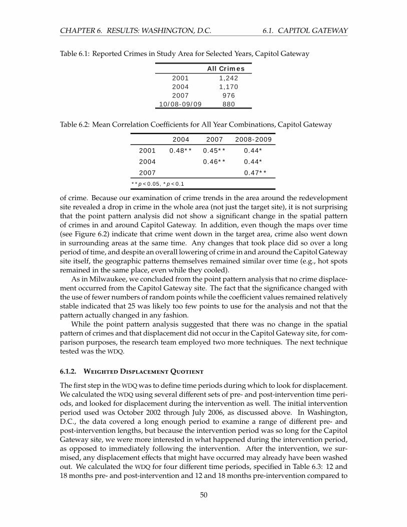
CHAPTER 6. RESULTS: WASHINGTON, D.C. 6.1. CAPITOL GATEWAY
Table 6.1: Reported Crimes in Study Area for Selected Years, Capitol Gateway
y
y
Capper Carrollsburg Original, 100 points
2005 2007 2008-20092002 0.50 ** 0.48 ** 0.46 **
2005 0.49 ** 0.41 *
2007 0.54 **
All Crimes, 25 points2004 2007 2008-2009
2001 0.49 0.43 0.452004 0.44 0.442007 0.48
All Crimes, 100 points2004 2007 2008-2009
2001 0.48 ** 0.46 ** 0.47 **2004 0.45 ** 0.45 **2007 0.47 **
All Crimes, 50 points
2004 2007 2008-20092001 0.48 ** 0.45 ** 0.44 *
2004 0.46 ** 0.44 *
2007 0.47 **
All Crimes2001 1,2422004 1,1702007 976
10/08-09/09 880
All Crimes2002 1,3612005 7902007 820
10/08-09/09 751
Table 6.2: Mean Correlation Coefficients for All Year Combinations, Capitol Gateway
2004 2007 2008-2009
2001 0.48** 0.45** 0.44*
2004 0.46** 0.44*
2007 0.47**
**p <0.05, *p <0.1
of crime. Because our examination of crime trends in the area around the redevelopmentsite revealed a drop in crime in the whole area (not just the target site), it is not surprisingthat the point pattern analysis did not show a significant change in the spatial patternof crimes in and around Capitol Gateway. In addition, even though the maps over time(see Figure 6.2) indicate that crime went down in the target area, crime also went downin surrounding areas at the same time. Any changes that took place did so over a longperiod of time, and despite an overall lowering of crime in and around the Capitol Gatewaysite itself, the geographic patterns themselves remained similar over time (e.g., hot spotsremained in the same place, even while they cooled).
As in Milwaukee, we concluded from the point pattern analysis that no crime displace-ment occurred from the Capitol Gateway site. The fact that the significance changed withthe use of fewer numbers of random points while the coefficient values remained relativelystable indicated that 25 was likely too few points to use for the analysis and not that thepattern actually changed in any fashion.
While the point pattern analysis suggested that there was no change in the spatialpattern of crimes and that displacement did not occur in the Capitol Gateway site, for com-parison purposes, the research team employed two more techniques. The next techniquetested was the WDQ.
6.1.2. Weighted Displacement Quotient
The first step in the WDQ was to define time periods during which to look for displacement.We calculated the WDQ using several different sets of pre- and post-intervention time peri-ods, and looked for displacement during the intervention as well. The initial interventionperiod used was October 2002 through July 2006, as discussed above. In Washington,D.C., the data covered a long enough period to examine a range of different pre- andpost-intervention lengths, but because the intervention period was so long for the CapitolGateway site, we were more interested in what happened during the intervention period,as opposed to immediately following the intervention. After the intervention, we sur-mised, any displacement effects that might have occurred may already have been washedout. We calculated the WDQ for four different time periods, specified in Table 6.3: 12 and18 months pre- and post-intervention and 12 and 18 months pre-intervention compared to
50

CHAPTER 6. RESULTS: WASHINGTON, D.C. 6.1. CAPITOL GATEWAY
Table 6.3: Weighted Displacement Quotient Results, Capitol Gateway
lengthType of crime t0 t1 measure 1000' 2000'All -1.383 2.917 3.577
12 mo. Personal 10/2001-09/2002 08/2006-07/2007 -1.071 1.395 1.864Property -1.790 3.919 4.750All -0.632 0.906 1.623
12 mo.* Personal 10/2001-09/2002 10/2002-09/2003 -0.800 0.940 1.858Property -0.034 -46.000 -60.000All -1.055 2.814 3.564
18 mo. Personal 04/2001-09/2002 08/2006-01/2008 -0.879 1.107 1.429Property -1.356 4.223 5.326All -0.416 -0.706 -1.181
18 mo.* Personal 04/2001-09/2002 10/2002-03/2004 -0.652 0.605 1.393Property 0.200 - -
Note: Intervention period: 10/2002-07/2006
*Searched for displacement during intervention period.
1000' 2000'All -1.38 2.92 3.58
Personal -1.07 1.39 1.86Property -1.79 3.92 4.75
All -0.63 0.91 1.62Personal -0.80 0.94 1.86Property -0.03 -46.00 -60.00
All -1.06 2.81 3.56Personal -0.88 1.11 1.43Property -1.36 4.22 5.33
All -0.42 -0.71 -1.18Personal -0.65 0.61 1.39Property 0.20 - -
Note: Intervention period: 10/2002-07/2006*Searched for displacement during intervention period.
18 mo.* 04/2001-09/2002 10/2002-03/2004
08/2006-01/2008
10/2002-09/2003
08/2006-07/200712 mo. 10/2001-09/2002
04/2001-09/2002
10/2001-09/200212 mo.*
18 mo.
Success measure
WDQPre/post length
Type of crimet0 t1
1000' 2000'
All -1.38 2.92 3.58Personal -1.07 1.39 1.86Property -1.79 3.92 4.75
All -0.63 0.91 1.62Personal -0.80 0.94 1.86Property -0.03 -46.00 -60.00
All -1.06 2.81 3.56Personal -0.88 1.11 1.43Property -1.36 4.22 5.33
All -0.42 -0.71 -1.18Personal -0.65 0.61 1.39Property 0.20 - -
Success measure
WDQPre/post length
Type of crimet0
(Pre-period)
t1
(Intervention or post-period)
08/2006-01/2008
10/2002-09/2003
08/2006-07/200712 mo. 10/2001-09/2002
04/2001-09/2002
10/2001-09/200212 mo.*
18 mo.
Note: Intervention period: 10/2002-07/2006*Searched for displacement during intervention period.
18 mo.* 04/2001-09/2002 10/2002-03/2004
12 and 18 months during the intervention. The WDQ was calculated for all crime, personalcrime and property crime.
As in Milwaukee, we searched for displacement in two buffers: a 1000’ buffer anda 2000’ buffer that were mutually exclusive. Table 6.3 provides the WDQ for each of thetime periods and buffers considered. The table also provides the success measure, or thedenominator, of the WDQ. WDQs were only calculated where the success measure wasnegative; if crime did not decrease during the study period, no displacement would beexpected.
The WDQ results for Capitol Gateway across all types of crime and time periods weremore consistent than for Milwaukee. All but one success measure was negative, indicatingthat for the most part, both property and personal crimes decreased in the redevelopmentsite over the study period. For both types of crime, the 12-month pre- and post-interventionperiods produced WDQs that were positive and greater than one, indicating that a diffusionof benefits took place and that the decreases in crime in the buffer areas were at least asstrong as the effects in the target area itself. When we compared crime levels for the 12months before and 12 months during the intervention, we found mixed results. For allcrime and personal crime, the WDQs were positive and at or greater than one, indicatingthat a diffusion of benefits took place immediately after the start of the intervention (whilethe redevelopment activities were continuing).
For property crimes, the success measure was negative but very near zero. The WDQsfor property crimes in both buffer areas were negative and very large. In their presentationof the WDQ, Bowers and Johnson (2003) cautioned that the measure should not be used toquantify the absolute amount of displacement that occurred, only the amount relative tothe target area; the large WDQ values should thus not be alarming. While the results forproperty crime during the first 12 months of the intervention indicated that displacementto the buffer areas did occur, the very small size of the success measure calls for caution ininterpretation of these specific WDQs.
Examining the crime trends in the two buffer areas for property crimes alone, we foundan increase in each buffer area from the first 12-month period to the second of approximately17 percent (46 crimes in the 1000’ buffer and 60 crimes in the 2000’ buffer). We also examinedthe crime trends in the target and comparison areas, and found that over the period, crimein both areas was stable, dropping by only one crime in the target area and remainingthe same in the comparison areas. In this case, then, value of the WDQ is effectively justthe total observed increase in crime in each of the buffer areas. Therefore, we do not take
51

CHAPTER 6. RESULTS: WASHINGTON, D.C. 6.1. CAPITOL GATEWAY
the large negative WDQs to be a strong indication that displacement of property crimesactually took place, but considered this result in concert with the results of the WDQs inother areas and time periods, and with the results of the other two methodologies. Becausethe success measure for property crimes for the 18-month intervention period was actuallypositive, indicating that crime increased in the target area over the study period, we didnot calculate WDQs for that area, but conclude that some displacement may have takenplace immediately following the start of redevelopment. However, that displacement waslater counteracted by a strong diffusion of benefits following the intervention.
The 18-month pre- and post-intervention periods yielded positive WDQs, providingadditional evidence that a diffusion of benefits from the Capitol Gateway site to nearbyareas took place. The 18-month pre- and during the intervention, however, revealedthat some displacement might have occurred: the all crimes category had negative WDQvalues less than negative 1. The personal crime category had small positive WDQ values,and the property crime category actually had a positive success measure, so no WDQswere calculated for that crime category. Taken together with the property crime resultsdiscussed above, it appears that any positive effects of the intervention on neighboringareas (i.e., diffusion of benefits) were lagged behind the actual intervention, possibly forseveral years. There may have been some displacement early on, but that disappeared asthe redevelopment progressed. In addition, the values of the WDQ were larger for the 2000’buffer, so that the effects did not ”wash out” towards the outer boundaries of the studyarea.
To summarize, the WDQ effort for Capitol Gateway had strong results, indicating adiffusion of benefits for most time periods and areas that was delayed until after theend of the intervention. The exceptions were the 12-month pre- and during interventionperiods for property crime and the 18-month pre- and during intervention periods for ”allcrime,” during which time some displacement of those crimes may have occurred. Thateffect, however, had disappeared by the end of the redevelopment period, by which pointdiffusion of benefits was observed.
6.1.3. Time Series Analysis
Single series ARIMA model The first step in the time series analysis was to analyze theeffects of the intervention in the redevelopment site alone in order to confirm and quantifythe decrease in crime in the redevelopment site that was identified through descriptivemeans outlined above. The first step in developing an ARIMA model was to specify theappropriate lag structure. In order to do this, we examined four monthly crime series ofinterest, looking at data for ”all crimes”: the Capitol Gateway site, the 1000’ and 2000’buffers, and the comparison area (Barry Farms). Augmented Dickey-Fuller tests indicatedthat all four series were stationary. We next estimated the ACF and PACF for the target andcomparison area series, and found them to be very similar.
Because of the similarity of the two series, the comparison area was used to determinelag length; we assumed that that series did not fundamentally change over the study perioddue to the intervention as the redevelopment site series likely did. If the intervention hadan impact on crime in the redevelopment site, then it would become difficult to identify theappropriate natural lag structure using the monthly crime series for the redevelopment siteitself. Ideally, if we had a series long enough pre-intervention, we could use that portionof the redevelopment site’s crime series to determine the lag structure; unfortunately, thedata available did not cover a long enough pre-intervention period. Using standard fit
52
CHAPTER 6. RESULTS: WASHINGTON, D.C. 6.1. CAPITOL GATEWAY
indices and diagnostics to evaluate possible model specifications, we determined that anAR(2) model, or an autoregressive model with two lags, was most appropriate for both theredevelopment site series and the comparison area series.1
The series of monthly crime in the redevelopment site and the comparison site weretested for seasonality based on observed but unexplained correlations in the residualsstarting at lag 6. In other words, crime for any given month was correlated to crime sixmonths prior, supporting the idea that crime rates change with the seasons. We added asix-month seasonal lag to the model in order to address this issue; the term was significantand improved the model’s performance.
The model thus included two lags for the monthly difference between the target andcomparison area, a seasonal dummy variable, and three intervention variables. The inter-vention dummy variables were included to delineate different time periods in the redevel-opment timeline. The four periods were:
Baseline, or pre-intervention: January 2000–September 2002
Move-out: October 2002–August 2006
Construction/move-in: September 2006–November 2008
Move-in/stability: December 2008–September 2009
Table 6.4 shows the results of the model estimations for both Capitol Gateway andBarry Farms. In the Capitol Gateway model, all three intervention coefficients were highlysignificant and all had virtually the same magnitude. The model suggests that each monthafter the intervention, the mean number of crimes per month was approximately fivecrimes lower than the site’s overall mean of 9.5 crimes per month. This is a large dropin crime, and indicates that the intervention was successful at reducing crime at the siteitself. Barry Farms, on the other hand, did not experience the same drop in crime duringthe intervention periods. Instead, crime was significantly higher in Barry Farms duringand following the intervention. Because Barry Farms was several miles from the CapitolGateway site, it was unlikely that the increase at Barry Farms was due to displacementof crime from the redevelopment activity at Capitol Gateway. The results from the BarryFarms site suggested that there may have been external factors pushing crime up in otherpublic housing areas, just as HOPE VI was underway at Capitol Gateway. The estimateddecrease in crimes from the Capitol Gateway model was thus probably conservative.
VAR The next step was to estimate a structural VAR using three series: the redevelopmentsite, the 1000’ buffer and the 2000’ buffer. The VAR model here had six possible directionaleffects: the redevelopment site on each buffer area, each buffer area on the target site, andeach buffer area on the other buffer. Following the process used for the Milwaukee site,we only estimated the contemporaneous effects of the outward directional effects, or thoseof the target on both buffers and the 1000’ buffer on the 2000’ buffer (lagged effects wereestimated in the inward and outward direction). The VAR results presented here includethe parameter estimates for both the lagged and the contemporaneous (no lag) effects(provided in Table 6.5).
As in Milwaukee, the model for the target area was very similar to that developed usingsingle series ARIMA results, and in the target area, crime dropped significantly following
1The first lag is crime one month prior and the second lag is crime two months prior.
53

CHAPTER 6. RESULTS: WASHINGTON, D.C. 6.1. CAPITOL GATEWAY
Table 6.4: Impact of Redevelopment on Capitol Gateway and Barry Farms, Washington,D.C.: Results of ARIMA Model for All Crime
b S.E. b S.E.Constant 9.50 0.83 6.51 0.66Autoregressive lag 1 0.25 0.09 0.10 0.09Autoregressive lag 2 0.18 0.09 0.24 0.09Seasonal dummy (6 mo.) -0.01 0.10 -0.28 0.09Move-out period -4.90 1.08 0.58 0.88Move-out/construction period -4.70 1.23 5.01 0.98Move-in period -5.64 1.62 8.91 1.40
**p <0.05, *p <0.10
Barry Farms
Capitol Gateway model: Dep. var = All crime, Capitol Gateway target area. Log likelihood = -288.97; AIC = 593.94
Barry Farms model: Dep. var = All crime, Barry Farms. Log likelihood = -301.6; AIC = 619.19
Capitol Gateway
** ****
****
**
*****
****
Table 6.5: Impact of Redevelopment of Capitol Gateway, Washington, D.C.: Results ofStructural VAR Model for All Crime
Constant 4.46 ** 1.62 1.94 3.58 21.42 ** 4.34Target area (no lag) - - 0.30 0.20 0.27 0.24AR Lag 1, Target area 0.20 ** 0.09 0.27 0.20 0.43 * 0.24AR Lag 2, Target area 0.19 ** 0.09 0.29 0.20 -0.37 0.241000' buffer (no lag) - - - - 0.39 ** 0.11AR Lag 1, 1000' buffer 0.09 ** 0.04 0.11 0.09 0.13 0.11AR Lag 2, 1000' buffer 0.00 0.04 0.08 0.09 0.01 0.11AR Lag 1, 2000' buffer -0.01 0.04 0.20 ** 0.08 0.17 * 0.10AR Lag 2, 2000' buffer -0.01 0.04 0.25 ** 0.08 0.16 0.10Move-out period -2.75 ** 0.89 -3.78 * 1.96 1.28 2.38Construction period -2.33 ** 0.94 -3.71 * 2.08 -1.10 2.52Stability period -2.71 ** 1.15 -4.86 * 2.54 -6.63 ** 3.08R-square
N=115, *p<0.10, **p<0.05
0.49 0.30
Target Area 1000' Buffer 2000' Buffer
Coeff Std Err Coeff Std Err Coeff Std Err
0.46
54

CHAPTER 6. RESULTS: WASHINGTON, D.C. 6.1. CAPITOL GATEWAY
the pre-intervention period. Two main results from the VAR are worth noting. First,there was a positive relationship between crime counts in each area and crime counts inthe surrounding areas. Thus, all else being equal, if crime rose in one area, it would beexpected to rise in all areas. It should be noted that all of the effects were relatively smalland only the 2000’ buffer had significant results (on the AR1 lag for the target area and thenon-lagged 1000’ buffer term) that measured crime moving ”outward.” The signs of mostof the estimates were positive, however, supporting the conclusion that if crime dropped inone area, it would drop in adjacent locations as well. This relationship was not surprising,as an extensive criminological literature, both theoretical and empirical, has tied crime ina given location to crime in surrounding areas. This finding also indicated that we shouldexpect positive spillover effects, or a diffusion of benefits, to areas surrounding CapitolGateway.
The second thing to note is that HOPE VI appeared to have decreased crime in all threeareas: directly in the target area and both directly and indirectly via changes in the targetarea, in the buffer areas. That is, HOPE VI decreased crime in Capitol Gateway, which ledto decreases in crime in the surrounding areas (because crime in Capitol Gateway waspositively correlated with crime in its neighboring areas), and HOPE VI decreased crimedirectly in the buffer areas, regardless of what happened in the target area (as indicated bythe significant coefficients on the time period dummies in both buffer areas). The resultsalso indicate that the effects were strongest in the target area and 1000’ buffer areas, andthose effects continued throughout the redevelopment period. Direct effects were felt lessstrongly in the 2000’ buffer and were significant only in the last period, move-in/stability.In fact, the effects in the 1000’ buffer were larger than for the target area. Finally, significanteffects were found in the 2000’ buffer only, indicating that the intervention’s effects slowlymoved outward from the target area during the study period.
Some of the measured impact of HOPE VI from the ARIMA model above did not comefrom HOPE VI’s direct impact on Capitol Gateway. Rather, at least some of the observedimpact came from an indirect feedback effect, where HOPE VI lowered crime in the sur-rounding areas, leading to lower crime in Capitol Gateway. In addition, the VAR modelindicated that the effects on the buffer areas were delayed and built over time throughoutthe redevelopment period. This result indicates again that the intervention became moreeffective over time, and supports the results of the WDQ, which indicated small effects—even displacement of property crimes early on—and diffusion of benefits at the end of andfollowing the intervention.
6.1.4. Conclusion
Two of the three methodologies applied in the Capitol Gateway case presented consistentresults. The point pattern analysis indicated that there was no change in the pattern ofcrimes prior to redevelopment compared to any period afterwards, suggesting that nodisplacement or diffusion occurred. As was discussed earlier, however, the method doesnot identify drops in crime if those drops do not result in a change in the overall pattern.That appeared to be the case here, as crime dropped throughout the study area used forthe point pattern analysis.
The other two methods provided evidence of diffusion of benefits, especially later inthe study period. The time series identified a significant average drop of approximatelyfive crimes per month during each different redevelopment period, indicating that HOPEVI was highly successful at decreasing the crime levels in the redevelopment site itself.
55

CHAPTER 6. RESULTS: WASHINGTON, D.C. 6.2. CAPPER/CARROLLSBURG
This was in addition to the trend in the comparison area that was actually increasing overthe study period, indicating that while crime at Capitol Gateway was decreasing, crimeat comparable sites elsewhere in the city was going up. The identified drop in crime,therefore, is likely a conservative estimate. The time series results thus confirmed what wefound through descriptive analyses: that it was appropriate to search for displacement ordiffusion based on the significant drop in crime at Capitol Gateway.
The WDQ effort revealed a possible initial displacement of property crime, especiallyduring the early months of the intervention. WDQs for later periods, however, showedsigns of diffusion of benefits to the buffer areas. The time series analysis did not pick up thedisplacement early in the redevelopment period, but those models took all crimes as thedependent variable, which may have masked the displacement of property crime alone.The VAR model, however, did provide support for the diffusion effects identified with theWDQs. Moreover, the VAR models revealed that the crime drop was strongest in the targetarea earlier in the study period, and the decrease diffused out to the 2000’ buffer closer tothe end of the study period.
The next section presents results for the last site under study, Capper/Carrollsburg.
6.2. CAPPER/CARROLLSBURG
Figure 6.3 displays the same redevelopment timeline shown above and includes line graphsof all crime in the four main study areas (the site, two displacement buffers, and thecomparison area—Syphax/Greenleaf Gardens). The figure also includes dotted lines thatdelineate the different study periods selected by the research team and explained in moredetail below in Section 6.2.3. The figure shows that crime in the site appeared to dropsignificantly in mid-2003 and that crime in the two buffers also dropped starting at thesame point, though not to the same degree as in the target area. Crime in the comparisonarea appeared to remain relatively stable throughout the study period, with recurrent peaksthroughout the period.
As in Milwaukee and the Capitol Gateway site, the intervention period was long, andthe Capper/Carrollsburg redevelopment had the longest timeline of the three sites underexamination. Again, this characteristic of such large-scale redevelopment projects makesit difficult to identify clear-cut start and end dates of the intervention. The interventionperiods, however, generally center around the period of July 2003 through December 2006,roughly the period of construction of the first senior building. The specific dates used asinterventions are specified with each analysis.
Figure 6.4 provides crime density maps for four selected years in the study period:2002, 2004, 2006, and 2008. The density maps were created using data covering a half-mileradius around the site in order to capture any hot spots that might be occurring nearby butjust outside the site boundaries. These maps were used purely for descriptive purposes,to provide an indication of the changes that took place in each site. The maps were notused as part of any statistical analyses, nor were they used alone to draw firm conclusionsregarding the changing crime patterns in and around the study sites. The maps revealthat the density of crime inside the site appeared to lessen with time. By 2008, most of thecrime hot spots appeared to have moved outside of the 2000’ buffer area. After 2002, thetarget area itself had a very low density of crime, but there was a stable hot spot just to thenorthwest of the site that remained there throughout the study period.
This examination of crime patterns revealed that crime decreased in the site following
56

CHAPTER 6. RESULTS: WASHINGTON, D.C. 6.2. CAPPER/CARROLLSBURG
Figu
re6.
3:R
edev
elop
men
tTim
elin
e,C
appe
r/C
arro
llsbu
rg,W
ashi
ngto
n,D
.C.
All Part I Incidents 2000
2002
2004
2005
2006
2007
2008
2009
2010
2001
2003
Cons
truct
ion
begi
ns,
seni
or b
uild
ing
Cons
truct
ion
begi
ns, t
ownh
ouse
s
Resid
ent r
eloc
atio
n fro
m C
appe
r site
Capp
er S
enio
r Bl
dg. #
1
com
plet
e
Occu
panc
y be
gins
in
tow
nhou
ses
HOPE
VI a
war
d gr
ante
d
Capp
er S
enio
r Bl
dg. #
2
com
plet
e
Seni
or b
ldgs
. at
stab
ility
19
59
77
17
Base
line
perio
dM
ove-
out p
erio
dD
emol
ition
/Co
nstr
uctio
n pe
riod
Stab
ility
per
iod
2000
’ Bu�
erSy
phax
/Gre
enle
af(c
ompa
rison
)
1000
’ Bu�
erA
rthu
r Cap
per/
Carr
olls
burg
Mov
e-in
per
iod
57
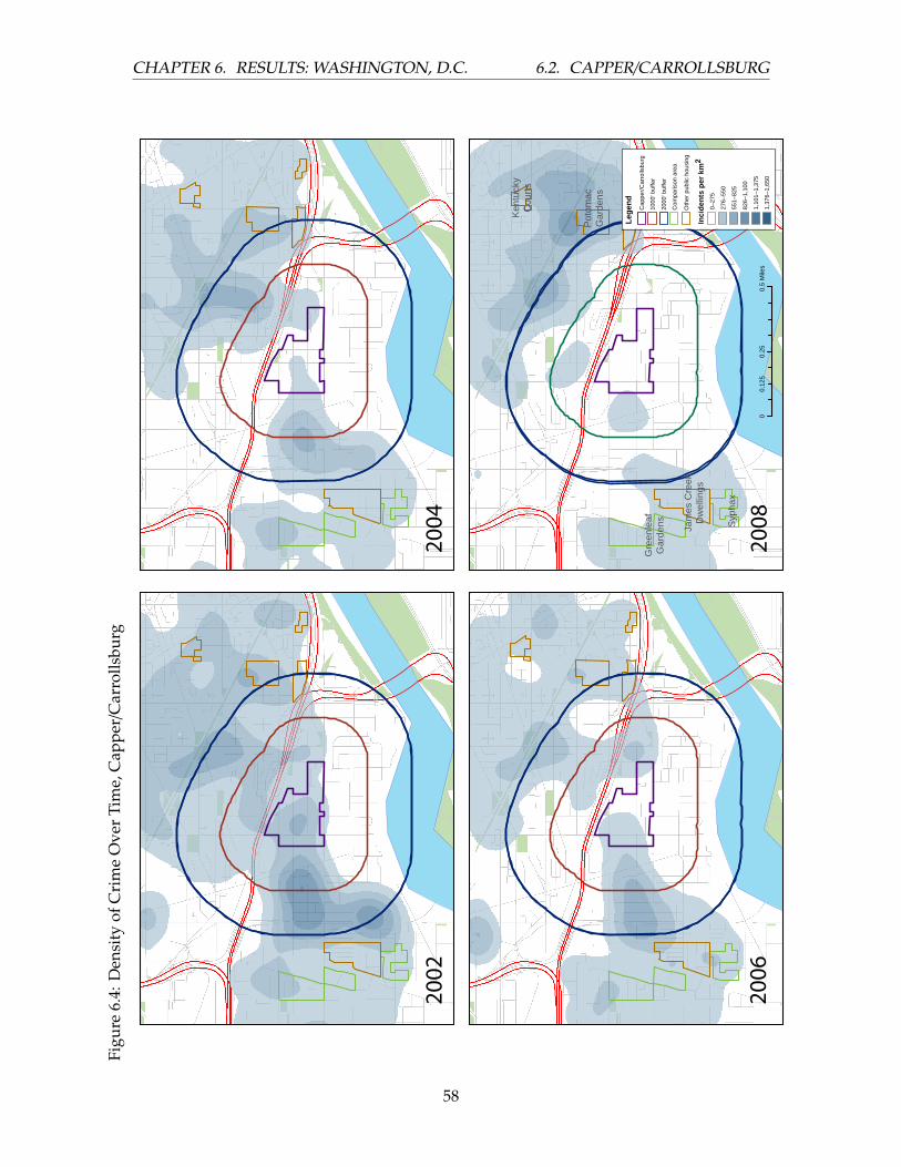
CHAPTER 6. RESULTS: WASHINGTON, D.C. 6.2. CAPPER/CARROLLSBURG
Figu
re6.
4:D
ensi
tyof
Cri
me
Ove
rTi
me,
Cap
per/
Car
rolls
burg
2002
2004
2006
2008
Lege
nd Capp
er/Ca
rrollsb
urg10
00' b
uffer
2000
' buff
erCo
mpari
son a
rea
Inci
dent
s pe
r km
2
0–27
5
Othe
r pub
lic ho
using
276–
550
551–
825
826–
1,100
1,101
–1,37
51,3
76–1
,650
00.2
50.5
0.125
Miles
Jame
s Cree
kDw
elling
s
Gree
nleaf
Garde
ns Syph
ax
Potom
acGa
rdens
Kentu
cky
Court
s
58

CHAPTER 6. RESULTS: WASHINGTON, D.C. 6.2. CAPPER/CARROLLSBURG
redevelopment activities, and that a search for possible displacement and diffusion wasappropriate. The actual decrease in crime was quantified via the WDQ and time seriesanalyses, presented below, but we started our consideration of displacement with pointpattern analysis.
6.2.1. Point Pattern Analysis
Point pattern analysis was used to determine whether the pattern of crimes in the areaswithin and around the Capper/Carrollsburg site changed, and the area examined for thisanalysis was the area within a half-mile of the site boundaries. Using a half-mile radiusaround the target area allowed us to capture any changes that occurred either within thetarget area boundaries or within a short distance of the boundaries; had we only used thetarget area itself, we would not have captured any crime displacement from the target siteto just beyond its borders that might have occurred.
The point pattern analysis started with the identification of time periods and crime typesto use for analysis. Because the redevelopment timeline was long, yearlong intervals wereused as the pre- and post-intervention time periods, comparing all crimes that occurredover one year before the redevelopment started to crimes that occurred in another full year,either during or after redevelopment. As with Capitol Gateway, the final year of data usedfor the point pattern analysis was the last full year of data, October 2008 through September2009. Table 6.6 provides each year that was used in the analysis and the number of crimes(all crimes) that occurred in the half-mile buffer area during that period. The Capper targetsite was small, with few enough crimes to allow us to look at the spatial patterns of allcrimes together.
Next, random point distributions were generated. First an appropriate number ofpoints was selected. As with the other two sites, we tested distributions with differentnumbers of random points each, including 25 points, 50 points, and 100 points. Witheach number of random points (25, 50, and 100), the point pattern process was repeated100 times, providing 100 different correlation coefficients for each possible combinationof years examined. The skew and kurtosis of each set of 100 correlation coefficients wereexamined, and both measures were less than one for all possible year and random pointnumber combinations examined. Because the results were so similar, only the results fromthe analyses using 100 random points are presented here.
Table 6.7 provides the mean correlation coefficients between crime patterns for eachyear combination examined using random point distributions of 100 points each. All butone year combination was highly positively correlated; the remainder were positive butsignificant only at the p<0.10 level. All correlation coefficients had values near 0.50, as didthe coefficients for the Capitol Gateway site. Because the correlations were all positive,even those that were not significant, we can conclude that the spatial pattern of crimes didnot change significantly across the study period, as was the case in the other two sites. Ourexamination of crime trends in the area around the redevelopment site revealed a drop incrime in the target area and persistent hot spots of crime outside the target area. Therefore,it is not surprising that the point pattern analysis did not show a significant change in thespatial pattern of crimes in and around Capper/Carrollsburg. We concluded from the pointpattern analysis that no crime displacement occurred from the Capper/Carrollsburg site.
59

CHAPTER 6. RESULTS: WASHINGTON, D.C. 6.2. CAPPER/CARROLLSBURG
Table 6.6: Reported Crimes in Study Area for Selected Years, Capper/Carrollsburg
y
y
Capper Carrollsburg Original, 100 points
2005 2007 2008-20092002 0.50 ** 0.48 ** 0.46 **
2005 0.49 ** 0.41 *
2007 0.54 **
All Crimes, 25 points2004 2007 2008-2009
2001 0.49 0.43 0.452004 0.44 0.442007 0.48
All Crimes, 100 points2004 2007 2008-2009
2001 0.48 ** 0.46 ** 0.47 **2004 0.45 ** 0.45 **2007 0.47 **
All Crimes, 50 points
2004 2007 2008-20092001 0.48 ** 0.45 ** 0.44 *
2004 0.46 ** 0.44 *
2007 0.47 **
All Crimes2001 1,2422004 1,1702007 976
10/08-09/09 880
All Crimes2002 1,3612005 7902007 820
10/08-09/09 751
Table 6.7: Mean Correlation Coefficients for All Year Combinations, Capper/Carrollsburg
2005 2007 2008-2009
2002 0.50** 0.48** 0.46**
2005 0.49** 0.41*
2007 0.54**
**p <0.05, *p <0.1
6.2.2. Weighted Displacement Quotient
While the point pattern analysis suggested that there was no change in the spatial patternof crimes and that displacement did not occur in the Capper/Carrollsburg site, the researchteam employed two other analysis techniques for comparison purposes. The next techniquetested was the WDQ.
The first step in the WDQ was to define time periods during which to look for displace-ment. We calculated the WDQ using several different sets of pre- and post-intervention timeperiods, and looked for displacement during the intervention as well. The initial interven-tion period used was July 2003 through February 2005, as discussed above. In Washington,D.C., the data covered a long enough period to examine a range of different pre- and post-intervention lengths, but, as with the Capitol Gateway site, we were interested in whathappened during the intervention period as well. We calculated the WDQ for four differenttime periods, specified in Table 6.8: 12 and 18 months pre- and post-intervention and 12and 18 months pre-intervention compared to 12 and 18 months during the intervention.The WDQ was calculated for all crimes, personal crime and property crime.
As in the two other sites, we searched for displacement in two buffers: a 1000’ bufferand a 2000’ buffer that were mutually exclusive. Table 6.8 provides the WDQ for each ofthe time periods and buffers considered. The table also provides the success measure, orthe denominator, of the WDQ. WDQs were only calculated where the success measure wasnegative.
The WDQ results for the Capper/Carrollsburg site were similar to those observed forCapitol Gateway. All success measures were negative, confirming that crime decreasedover the study period. The results consistently indicated that a diffusion of benefits tookplace from the site, with two exceptions. First, for personal crimes during the first 12months after the intervention period, the WDQ was negative. The same was true for the 18-month period following redevelopment for personal crimes. This pattern is similar to thatobserved for property crimes in Capitol Gateway, where a displacement effect was notedsoon after the intervention started that disappeared with time following the intervention.It is unclear why this result occurred, but one thing to note is that in both of these instances,the success measure was very low, which could very well have skewed the results. One
60

CHAPTER 6. RESULTS: WASHINGTON, D.C. 6.2. CAPPER/CARROLLSBURG
Table 6.8: Weighted Displacement Quotient Results, Capper/Carrollsburg
Pre/postlength
Type of crime
t0 t1Successmeasure
WDQ1000' 2000'
All -1.072 3.198 3.37912 mo. Personal 07/2002-06/2003 12/2004-11/2005 -0.381 0.125 -3.258
Property -2.488 4.118 5.250All -0.838 2.004 1.729
12 mo.* Personal 07/2002-06/2003 07/2003-06/2004 -0.451 1.496 1.994Property -1.711 2.682 2.464All -1.040 3.045 3.100
18 mo. Personal 01/2002-06/2003 03/2005-08/2006 -0.539 0.765 -0.739Property -1.958 4.077 4.880All -0.843 1.657 0.843
18 mo.* Personal 01/2002-06/2003 07/2003-12/2004 -0.539 1.088 1.402Property -1.337 2.103 0.701
Note: Intervention period: 07/2003-02/2005*Searched for displacement during intervention period.
1000' 2000'
All -1.072 3.198 3.379Personal -0.381 0.125 -3.258Property -2.488 4.118 5.250
All -0.838 2.004 1.729Personal -0.451 1.496 1.994Property -1.711 2.682 2.464
All -1.040 3.045 3.100Personal -0.539 0.765 -0.739Property -1.958 4.077 4.880
All -0.843 1.657 0.843Personal -0.539 1.088 1.402Property -1.337 2.103 0.701
Success measure
WDQPre/post length
Type of crime
t0
(Pre-period)
t1
(Intervention or post-period)
12 mo.*
12 mo. 07/2002-06/2003 12/2004-11/2005
07/2003-06/200407/2002-06/2003
07/2003-12/200401/2002-06/2003
Note: Intervention period: 07/2003-02/2005*Searched for displacement during intervention period.
18 mo.*
18 mo. 03/2005-08/200601/2002-06/2003
other factor to note in interpreting these findings is that other redevelopment projects weretaking place in the larger area, and may have accounted for the apparent diffusion effectsnoted in this site.
To summarize, the WDQ effort for Capper/Carrollsburg had the strongest, most con-sistent results of the three sites. The WDQs showed a diffusion of benefits across severaldifferent time periods, and in both the 1000’ and 2000’ buffers. Contextual knowledge ofthe greater redevelopment area invites caution in interpreting these findings.
6.2.3. Time Series Analysis
Single series ARIMA model The first step in developing the Capper/Carrollsburg ARIMAmodel was to specify the appropriate lag structure. In order to do this, we examined fourmonthly crime series of interest, looking at data for ’all crimes’: the Capper/Carrollsburgsite, the 1000’ and 2000’ buffers, and the comparison area (Syphax/Greenleaf Gardens).Augmented Dickey-Fuller tests indicated that all four series were stationary. We next esti-mated the ACF and PACF for the redevelopment site and the comparison area but did notfind them to be comparable. Thus, the lag structure for each series had to be determinedindependently. Using standard fit indices and diagnostics to evaluate possible model spec-ifications for the target and comparison area series, we determined that an ARMA(1,1)model—a model with one autoregressive lag2 and one moving average lag—was mostappropriate for the redevelopment site series. An AR(3) model—one with three autore-gressive lags—was found most appropriate for modeling the comparison area series.3
The series of monthly crime in the redevelopment site and the comparison site weretested for seasonality using the same six-month seasonality term that was used for CapitolGateway. The inclusion of that term did not improve the redevelopment site model,however. We also tested the inclusion of a seasonal dummy indicating whether it wassummer or winter; this did not improve that model either. Therefore, we decided notto include a seasonal term in the redevelopment site model. We tested the same termson the comparison area series, however, and found that instead of a six-month seasonallag, a five-month seasonal lag was significant. We also found that a dummy identifying
2The lag is crime one month prior.3The first lag is crime one month prior, the second lag is crime two months prior, and the third is crime
three months prior.
61

CHAPTER 6. RESULTS: WASHINGTON, D.C. 6.2. CAPPER/CARROLLSBURG
the three winter months (December, January, and February) and a dummy identifying thethree summer months (June, July, and August), were significant. Those three seasonalityterms were thus included in the model.
The redevelopment site model thus included one autoregressive lag and one movingaverage lag and four dummy variables indicating intervention time period. The compari-son site model included three autoregressive lags, a five-month seasonal lag, a dummy forwinter and for summer, and the four dummy variables indicating intervention time period.Five distinct periods were identified for the Capper/Carrollsburg site. Those periods were:
Baseline, or pre-intervention: January 2000–June 2003
Move-out: July 2003–March 2005
Demolition/construction: April 2005–December 2006
Move-in: January 2007–June 2008
Stability: July 2008–September 2009
Table 6.4 shows the results of the model estimations for both Capper/Carrollsburg andSyphax/Greenleaf Gardens. In the Capper model, all parameter estimates were highlysignificant. The four intervention terms were all negative, indicating that crime droppedat the site immediately following the start of redevelopment and continuing throughoutthe redevelopment period. The model suggests that each month after the intervention, themean number of crimes per month was between approximately 4 crimes and 6.75 crimeslower than the site’s overall mean of 8.5 crimes per month. This is a large drop in crime,and indicates that the intervention was successful at reducing crime at the site itself. Onepoint to note regarding this finding is that while a drop in crime is a sign of success, theCapper timeline was also the longest, meaning that it had the longest period of time of allthree sites considered with few residents on site. This likely played a role in keeping crimeat the actual site low while redevelopment was taking place.
The moving average term was also found to be significant in the Capper model. Onepossible explanation for this is that the police may have been highly responsive to significantcrime events in the Capper area. The moving average term would pick up that increasedactivity. For example, if there was a sudden shock in June (e.g., a rash of burglaries) andthere were three more crimes for that month than expected, in July, there would be twofewer crimes than expected. This might be explained by a police presence defined by quickresponsivity to serious crime events. Based on our knowledge of the overall area, whichincluded redevelopment of the baseball stadium, increased construction, and developmentof office and retail space and market-rate housing, it is plausible that the police aroundCapper/Carrollsburg were more responsive throughout the study period.
In the comparison site, only one of the intervention terms was significant: the stabilityperiod. The other intervention terms were not significant. All four parameter estimatesfor the intervention dummies, regardless of significance, were negative, as was the case inthe Capper/Carrollsburg model. They were, however, smaller in magnitude. The resultsof the comparison area indicate that it did not experience the same dramatic drop in crimeduring the redevelopment period that Capper/Carrollsburg did, providing more evidencethat the crime drop in the target areas was connected to the redevelopment activities takingplace there.
62

CHAPTER 6. RESULTS: WASHINGTON, D.C. 6.2. CAPPER/CARROLLSBURG
Table 6.9: Impact of Redevelopment on Capper/Carrollsburg and Syphax/Greenleaf,Washington, D.C.: Results of ARIMA Model for All Crime
b S.E. b S.E.Constant 8.52** 0.57 7.90** 0.67Autoregressive lag 1 0.76** 0.23 0.21** 0.09Autoregressive lag 2 - - 0.07 0.10Autoregressive lag 3 - - -0.21** 0.10Moving average lag 1 -0.68** 0.26 - -Seasonal lag (5 mo.) - - 0.20* 0.10Winter dummy - - -0.79 0.79Summer dummy - - 2.60** 0.79Move-out period -3.91** 0.97 -1.48 0.99Construction period -5.26** 0.97 -1.24 0.99Move-in period -6.76** 1.01 -1.42 1.05Stability period -5.82** 1.08 -1.95** 1.12
**p <0.05, *p <0.10
Capper/Carrollsburg Syphax/Greenleaf
Capper model: Dep. var = All crime, Capper/Carrollsburg target area; Log likelihood = -288.66; AIC = 593.31.Syphax model: Dep. var = All crime, Syphax/Greenleaf; Log likelihood = -287.78; AIC = 599.56
VAR The next step was to estimate a structural VAR using three series: the redevelopmentsite, the 1000’ buffer, and the 2000’ buffer. The VAR model had six possible directional effects:the redevelopment site on each buffer area, each buffer area on the target site, and eachbuffer area on the other buffer. Following the process used for the other two sites, weonly estimated the contemporaneous effects of the outward directional effects, or thoseof the target on both buffers and the 1000’ buffer on the 2000’ buffer (lagged effects wereestimated in the inward and outward directions). The VAR results presented here includethe parameter estimates for both the lagged and the contemporaneous (no lag) effects(Table 6.10).
As in the other two sites, the VAR model for the target area was similar to that producedby the ARIMA modeling. The most notable finding from the Capper/Carrollsburg VARmodel was that the intervention produced large, statistically significant, and surprisinglyconsistent direct effects in all three areas—this means the intervention affected crime ineach area regardless of what happened in the other two areas. In fact, the results seemedto indicate that the intervention had much larger direct effects on the buffers than it did onthe target area: the effect was three times larger in the 2000’ buffer than in the target area.While this may at first seem counterintuitive, crime in the buffers was higher than in thetarget area to begin with, so larger drops in crime were likely similar to or smaller than thedrop in the target area percentage-wise.
The results also revealed that the target area had a significant effect on both buffer areas,and in fact, the significant and negative coefficient for the target area term indicates thatthe target area had a negative effect on the 1000’ buffer: when crime went down in thetarget area, it went up in the 1000’ buffer. The effect was very small, however (less thanone crime), and the lagged target area terms were not significant. Therefore, while thesignificant negative coefficient could be a sign of displacement, the results also indicate
63

CHAPTER 6. RESULTS: WASHINGTON, D.C. 6.2. CAPPER/CARROLLSBURG
Table 6.10: Impact of Redevelopment of Capper/Carrollsburg, Washington, D.C.: Resultsof Structural VAR Model for All Crime
Constant 6.16 ** 1.80 16.15 ** 4.76 28.29 ** 5.85Target area (no lag) - - -0.29 ** 0.06 0.38 ** 0.20AR Lag 1, Target area 0.13 0.09 0.21 0.24 -0.26 * 0.30AR Lag 2, Target area 0.12 0.09 0.07 0.23 -0.15 0.291000' buffer (no lag) - - - - -0.48 0.30AR Lag 1, 1000' buffer 0.02 0.04 0.29 ** 0.12 0.37 0.14AR Lag 2, 1000' buffer -0.10 ** 0.04 0.05 0.12 0.15 ** 0.14AR Lag 1, 2000' buffer 0.09 ** 0.04 0.04 0.10 0.24 0.12AR Lag 2, 2000' buffer -0.04 0.03 -0.04 0.09 -0.04 * 0.11Move-out period -3.24 ** 0.95 -8.70 ** 2.52 -8.91 3.10Construction period -3.98 ** 1.13 -6.63 ** 2.99 -12.03 ** 3.68Move-in period -4.79 ** 1.38 -7.04 * 3.64 -16.75 ** 4.47Stability period -4.43 ** 1.31 -9.13 ** 3.47 -15.64 ** 4.27R-square
N=115, *p<0.10, **p<0.05
0.660.51
2000' Buffer
Coeff Std Err Coeff Std Err Coeff Std Err
Target Area 1000' Buffer
0.55
that any displacement was short-term and small. The target area’s effect on the 2000’ bufferwas the opposite—it was significant and positive, supporting the idea that diffusion ofbenefits took place. Again, though, the effect was very small and short-term.
Aside from these two significant coefficients, the models reveal that the target area didnot have a strong effect on either buffer area—the three areas were relatively unconnectedand their crime rates did not appear to co-vary. While this is an important finding, it shouldalso be interpreted with caution. The Capper/Carrollsburg site was located in a larger areaof investment and redevelopment, including new federal buildings and the new Nationalsbaseball stadium. Therefore, with the results of this modeling effort alone, it is difficult toattribute the direct effects found in the buffer areas to HOPE VI itself. Additional informationon the timing of other redevelopment projects would be needed in order to account fortheir possible confounding effects in the buffers.
Overall, while the effects in the buffer area may not have been due to HOPE VI, the effectsin the target area (discussed above in the ARIMA time series section) were at least partiallydriven by the redevelopment efforts on the site. In addition, the VAR results indicate thatany displacement was unlikely, indicating that at least part of the drop in crime on site wasa true drop in crime, and did not simply serve to move crime to another location.
6.2.4. Conclusion
The Capper/Carrollsburg site produced the most consistent results of all sites, and thoseresults were fairly similar to the results from the Capitol Gateway analysis. The pointpattern analysis did not reveal any changes in the pattern of crime, which was not surprisinggiven the persistent hot spots outside the buffer areas throughout the study period, asidentified in Figure 6.4. The WDQs were consistent, indicating a diffusion of benefitsthroughout the study period and for both the 1000’ and 2000’ buffers.
The time series analysis confirmed the noted drop in crime in the site, and the drop incrime over the study period was found to be large. This may have partially been a functionof the long redevelopment timeline and extended period with few residents on site; that
64

CHAPTER 6. RESULTS: WASHINGTON, D.C. 6.2. CAPPER/CARROLLSBURG
period of lower resident numbers was longest in Capper/Carrollsburg of all three sites.The comparison area, however, did not experience a similar decline, and the comparisonarea was located just outside the 2000’ buffer, in the area of additional redevelopment notassociated with HOPE VI. This points to HOPE VI as a likely driver of the changes in crimelevels observed in Capper/Carrollsburg.
The VAR model revealed some interesting results not observed in the other two sites:crime levels in any of the three areas (target area, 1000’, and 2000’ buffers) did not stronglyco-vary. That is, the crime levels in each of the three areas appeared to operate indepen-dently of what was happening in the other two sites. The parameter estimates in the VARwere in the right direction, indicating that a positive relationship between crime levels inthe three areas might have existed, but the estimates were small and for the most part,non-significant. The VAR also revealed that HOPE VI had apparent direct effects on all threeareas; its effects did not simply work through the improvements observed in the targetarea. While counter-intuitive, these direct effects are best understood in the context of thelarger, non-HOPE VI redevelopment projects taking place throughout the Near Southeastneighborhood, in which Capper/Carrollsbug was located. This supports the conclusionsof Zielenbach and Voith (2010) in their study of HOPE VI in Boston and Washington, D.C.
65

Chapter 7
Discussion and Conclusions
7.1. RESULTS BY SITE
The results presented above provide mixed evidence as to whether crime was displacedfrom the HOPE VI sites included in this study and other similar large-scale public housingredevelopment efforts, and the three methodologies did not always agree. Overall, how-ever, the results indicated very positive results in the target areas themselves, and someother positive changes in areas surrounding those sites, although those may have beendelayed for several months to several years.
7.1.1. Milwaukee
The results from Milwaukee were the most mixed, with evidence of crime displacementprovided by some of the WDQs. Table 7.1 provides a summary of the WDQ values for eachsite for each buffer (1000’ and 2000’). This table is simply the count of all WDQs that fellinto each range (less than -1, -1 to 1, and greater than 1). Numbers smaller than -1 indicatedisplacement, and numbers greater than 1 indicate diffusion of benefits. This table doesnot differentiate between different types of crime.
Only about half of the success measures for the different crime type/buffer/time periodcombinations studied in Milwaukee were negative and indicated that crime decreasedin the target area (see Table 5.3). All of the success measures, however, were near zero,indicating that the effects—whether positive or negative—were minimal. The fact thatthe success measures were all positive for the 18-month pre/post-intervention WDQ is anindication that the redevelopment’s reduction effects on crime grew with time and werestronger later in the study period. The WDQs provided evidence of some displacementof personal crimes—starting just after the intervention period ended—but that effect gotsmaller with increased time from the intervention period.
The time series analysis supported the finding that the effects of the intervention, whilegenerally serving to decrease crime over the study period, were delayed. In fact, the timeseries suggested that a significant drop in crime at the site did not occur until after theintervention, during the move-in/stability period. It should be noted that the interventionperiod chosen for this research encompassed the construction of Highland Gardens only—because the construction period was so long, we decided to identify the construction forthe first building as the ”intervention,” arguing that once major changes were made in onepart of the site, changes would follow more quickly in other parts of the site. In otherwords, even though the other buildings (Cherry Court and the scattered sites) hadn’t yet
66
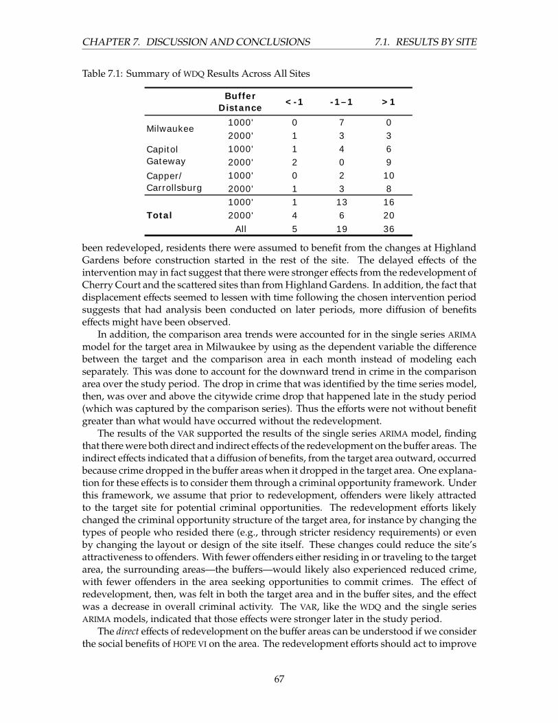
CHAPTER 7. DISCUSSION AND CONCLUSIONS 7.1. RESULTS BY SITE
Table 7.1: Summary of WDQ Results Across All Sites
Buffer Distance
<-1 -1–1 >1
1000' 0 7 02000' 1 3 31000' 1 4 62000' 2 0 91000' 0 2 102000' 1 3 81000' 1 13 162000' 4 6 20
All 5 19 36
Milwaukee
Capitol Gateway
Capper/ Carrollsburg
Total
been redeveloped, residents there were assumed to benefit from the changes at HighlandGardens before construction started in the rest of the site. The delayed effects of theintervention may in fact suggest that there were stronger effects from the redevelopment ofCherry Court and the scattered sites than from Highland Gardens. In addition, the fact thatdisplacement effects seemed to lessen with time following the chosen intervention periodsuggests that had analysis been conducted on later periods, more diffusion of benefitseffects might have been observed.
In addition, the comparison area trends were accounted for in the single series ARIMAmodel for the target area in Milwaukee by using as the dependent variable the differencebetween the target and the comparison area in each month instead of modeling eachseparately. This was done to account for the downward trend in crime in the comparisonarea over the study period. The drop in crime that was identified by the time series model,then, was over and above the citywide crime drop that happened late in the study period(which was captured by the comparison series). Thus the efforts were not without benefitgreater than what would have occurred without the redevelopment.
The results of the VAR supported the results of the single series ARIMA model, findingthat there were both direct and indirect effects of the redevelopment on the buffer areas. Theindirect effects indicated that a diffusion of benefits, from the target area outward, occurredbecause crime dropped in the buffer areas when it dropped in the target area. One explana-tion for these effects is to consider them through a criminal opportunity framework. Underthis framework, we assume that prior to redevelopment, offenders were likely attractedto the target site for potential criminal opportunities. The redevelopment efforts likelychanged the criminal opportunity structure of the target area, for instance by changing thetypes of people who resided there (e.g., through stricter residency requirements) or evenby changing the layout or design of the site itself. These changes could reduce the site’sattractiveness to offenders. With fewer offenders either residing in or traveling to the targetarea, the surrounding areas—the buffers—would likely also experienced reduced crime,with fewer offenders in the area seeking opportunities to commit crimes. The effect ofredevelopment, then, was felt in both the target area and in the buffer sites, and the effectwas a decrease in overall criminal activity. The VAR, like the WDQ and the single seriesARIMA models, indicated that those effects were stronger later in the study period.
The direct effects of redevelopment on the buffer areas can be understood if we considerthe social benefits of HOPE VI on the area. The redevelopment efforts should act to improve
67

CHAPTER 7. DISCUSSION AND CONCLUSIONS 7.1. RESULTS BY SITE
the behavior of residents and other individuals on site, reducing their criminal activity.HOPE VI efforts include the provision of additional social services, and are intended notonly to improve the physical conditions of the site itself but to assist residents in improvingthe quality of their lives through job skills training, educational opportunities, substanceabuse and mental health treatments, and other needed services. Through these services,the redevelopment efforts should be expected to reduce the criminal activity of residentswho live on site, making them less likely to commit crimes both in the target area andin nearby areas. In addition, with stricter criteria for residents who live in HOPE VI units,individuals on site are expected to be more responsible and less likely to commit crimes,regardless of whether they were previously residents of the site and accessed extensiveservice through HOPE VI or were simply new residents who met the more stringent criteria.In either case, the individuals in the target site would be less likely to commit crimes, andwould be less likely to commit crimes in nearby areas, reducing the levels of crime in thebuffer areas.
The delay in effects suggested by both the WDQ and the time series models shouldnot be seen as a negative result of the redevelopment efforts. Instead, the Milwaukee siteprovided the purest assessment of the effects of the physical site changes on crime becausethe residents on site were largely the same before and after the intervention. The delay inthe crime decrease identified supports the idea that it takes time for the physical changesto manifest themselves as changes in the quality of life in the area, here measured viacrime levels. And when those changes started to take place, the effects got stronger andstronger—crime in the redevelopment site continued to drop at a faster pace to the end ofthe study period (see Figure 5.3). This is an important finding that helps to highlight thesuccess of physical redevelopment alone.
7.1.2. Capitol Gateway
The results from Capitol Gateway were much more consistent than those from Milwaukeein that the different methods employed produced similar results. The initial descriptiveanalysis of crime in the site showed an obvious drop in crime starting at the beginning ofredevelopment; a concurrent drop did not occur in the comparison area and it appearedthat the buffers experienced smaller drops that occurred later in the study period. The pointpattern analysis did not reveal any changes in the pattern of crimes from the period prior toredevelopment to the period following redevelopment. Table 7.1 indicates that the CapitolGateway site had more large and positive WDQs than neutral or negative WDQs, providingevidence that diffusion of benefits took place. The WDQs indicated that the results variedwith type of crime but the success measures were all negative, indicating a drop in crimein the target area. Property crimes in particular showed evidence of displacement early inthe redevelopment period, but after the redevelopment period, showed strong evidenceof diffusion of benefits. The initial displacement may have been an immediate reactionto the redevelopment activities that dissipated after all residents moved out and the sitewas empty. The success of the redevelopment efforts is found more in the consideration ofcrime at the site when residents move back in, and during that period, the WDQs all pointedto a diffusion of benefits. Results for personal crime and ”all crime” also showed evidenceof a diffusion of benefits, and that diffusion started immediately after redevelopment.
In Washington, D.C., more so than in Milwaukee, the residents of the redeveloped sitewere likely different than those who moved out prior to redevelopment. In all sites, and inHOPE VI in general, criteria to move into a redeveloped or new unit are much stricter than
68

CHAPTER 7. DISCUSSION AND CONCLUSIONS 7.1. RESULTS BY SITE
for other public housing. This results in residents who are more likely to be ”successful”—at maintaining a housing unit, finding and maintaining employment, or participating ingovernance of the development (as is required in Milwaukee). While we were not able tocollect any data on residents’ characteristics, we assume that with these kinds of stricterresident criteria in all three sites came less criminally inclined residents, and residentswho had higher stakes in maintaining the safety and quality of their housing. The resultsobserved in the Capitol Gateway site, then, where diffusion of benefits increased afterresidents moved back in, is likely one manifestation of the stricter resident criteria.
The time series analyses supported the WDQ findings; the models showed a significantand large drop in crime in the target area that was not experienced in the comparison area.The success of HOPE VI in reducing crime on site is even more remarkable when the increasein crime that the comparison area experienced over the same time period is considered;the drop in crime at the HOPE VI site occurred despite an increase in crime in similar siteselsewhere in the city. This is an indication that our findings quantifying the drop in crimeare likely on the conservative side for Capitol Gateway.
The VAR results pointed to a diffusion of benefits from the target area to the buffer areas.The strongest effects were found in the 1000’ buffer, and the 2000’ buffer experienced smallbut significant drops in crime later in the study period. Because the time series modelsused ”all crimes” as the dependent variable, no displacement of crime was identified earlyin the period (as was the case for property crimes according to the WDQs). The use ofall crimes as the dependent variable may have served to mask the effects for propertycrime alone. As in Milwaukee, the HOPE VI efforts at the Capitol Gateway site werefound to have both indirect and direct effects on the buffer areas, and the same argumentsmade above regarding both the criminal opportunity structure of the site before and afterredevelopment and the criminal behavior of residents and other individuals on site beforeand after redevelopment both apply to Capitol Gateway as well.
Overall, the results found very positive effects in and around Capitol Gateway from theHOPE VI efforts. With more family units occupied each month, and additional redevelop-ment starting to take place in other areas surrounding the site, the benefits can be expectedto continue for some time.
7.1.3. Capper/Carrollsburg
Like those from Capitol Gateway, the results from Capper/Carrollsburg were very similaracross methods, and the results were similar to the findings from Capitol Gateway as well.All of the success measures calculated as part of the WDQ analysis were negative, indicatingthat crime did drop in the site during and after redevelopment. Nearly all of the WDQsthemselves were positive, indicating that a diffusion of benefits took place from the targetarea to the buffers. Many of those WDQs were also larger than one, pointing to a largepositive effect in the buffer areas (see Table 7.1).
The time series analysis confirmed the drop in crime identified through descriptive tech-niques and the WDQ. Similar to Capitol Gateway, crime at Capper/Carrollsburg droppedsignificantly and by a large amount each month, starting in the resident move-out period.The largest average monthly drops in crime occurred during the resident move-in period,with the second largest drops occurring in the stability period. In addition, the VAR re-vealed that the buffer areas experienced crime drops over the study period but that thosedid not appear to be associated with drops in the target area. Instead, the model indicatedthat the intervention itself affected crime in the buffers. These results are likely a result
69
CHAPTER 7. DISCUSSION AND CONCLUSIONS 7.1. RESULTS BY SITE
of the larger, non-HOPE VI redevelopment projects taking place in the neighborhood ofCapper/Carrollsburg.
Two important details of the Capper/Carrollsburg site should be kept in mind in inter-preting the results. First, the timeline for both of the Washington, D.C., sites was muchlonger than for the Milwaukee site, meaning those sites had a longer time period withfewer residents on site. Given the lack of residents on site, combined with the constructionefforts at each site—making the site unattractive in terms of criminal opportunity—it is notsurprising that crime dropped earlier at the Washington, D.C., sites than in Milwaukee,where residents on site throughout redevelopment.
A second important feature of the Capper/Carrollsburg site, mentioned above, wasthe large amount of redevelopment not associated with HOPE VI that was going on inthe area immediately surrounding the site. These efforts should have served to decreasecriminal opportunity there, as well, preventing much displacement from taking place tothe buffer zones surrounding the Capper/Carrollsburg site. Moreover, the redevelopmenttaking place in addition to HOPE VI can help to explain the interesting finding of a directintervention effect on the buffers; it is more likely that the effect was the result of theother redevelopment, not the effect of HOPE VI itself. Therefore the VAR results should beinterpreted with caution.
7.1.4. Summary of Results
The first two research questions, then, were answered through the analytic methods pre-sented above. The first question, ”Does the closing of a large high-poverty public housingdevelopment under HOPE VI influence patterns of crime in and around that development,and if so, how?” can be answered in the affirmative. We found a clear indication in allthree sites that crime dropped at some point during redevelopment and that redevelopmentaffected crime in surrounding areas in some way—usually by decreasing it. The effectsin the buffers varied, but for the most part, we observed a diffusion of benefits from thetarget sites outward. Additional investigation into subtypes of crime would help to bringmore specificity to the results (e.g., whether any crime prevention methods implementedduring redevelopment should target specific types of crimes that are more vulnerable todisplacement).
The second question, ”Does crime displacement or diffusion of benefits result duringthe time that the development is closed for rebuilding, and does crime return to previouslevels when the development reopens?” was also answered fairly consistently across allthree sites. As just stated, we found a consistent pattern of diffusion of benefits from suchlarge-scale public housing redevelopment efforts. In addition, in no site did we find anyreturn to pre-intervention crime levels following the intervention period. This indicatesthat the positive effects—the drops in crime—lasted at least as long as the study period,which was generally one to two years beyond the end of the intervention period in each site.It should be noted that with a small ”post” period in each site, this study may have capturedonly the initial positive benefits of redevelopment. If those results were not maintainedor did not last past the initial first wave of residents, that degradation of benefits was notcaptured. In other words, it may be that the first wave of residents who move into a newsite are successful, but that once resident turnover begins—which is common in publichousing units—the second wave of residents may not be as successful or the criteria maynot be enforced as strictly, leading to conditions on the site slowly regressing to their initialstate. While we have no evidence that this happened in any of the sites, this represents a
70

CHAPTER 7. DISCUSSION AND CONCLUSIONS 7.2. METHOD COMPARISON
note of caution in interpreting the results based on the short post-intervention length.
7.1.5. Challenges
This research has highlighted many of the difficulties associated with the study of displace-ment in this context—from large-scale public housing redevelopment sites. Most previ-ous displacement studies have focused on interventions associated with problem-orientedpolicing strategies, such as enhanced enforcement in a hot spot, or a small geographic area.Those types of interventions are usually short-term in nature, have clear start and enddates, and target clearly defined, small sites. The difficulties with applying the techniquesand theories from that type of study to one like this where the intervention is long-termand takes place over a large geographic area should not be ignored. First, identifying thespecific period of intervention is difficult—here, in each site we did our best to use theredevelopment timeline to make educated decisions about when the most intense changeson site occurred, and used that period as our intervention. In Milwaukee, where residentswere on site while redevelopment took place, this was difficult, and we chose constructionof the first new building as our intervention period. In Washington, D.C., where residentswere not on site during redevelopment, we chose the period when residents were not onsite as our intervention period.
Second, choosing the boundaries of the sites proved difficult, especially in Milwaukee,where one redevelopment project bled into another, and the process of redevelopment foreach building or unit was intertwined with the others. We necessarily chose a large targetsite to encompass all redevelopment activities in Milwaukee, but the results indicated thatthere may have been differential effects from the redevelopment of each portion of the largersite (e.g., the effects of changes to Cherry Court may have been different from the effects ofchanges at Highland Gardens; see Section 7.1.1). In Washington, D.C., public housing sitedefinition was more straightforward, but for Capper/Carrollsburg, nearby redevelopmentefforts made the actual boundaries of redevelopment efforts difficult to identify.
Finally, identifying areas of possible displacement was also difficult. Resident data arenotoriously hard to collect from housing authorities, and, while the two housing authori-ties consulted for this research were extremely helpful, we did not get any information onspecific residents, including demographics or where residents moved when they were relo-cated from the site pre-redevelopment. This limited our ability to include any demographicdata in the statistical models and to identify possible locations of crime displacement otherthan the buffer zones.
Nonetheless, studying displacement from public housing is an important undertaking,and the possibility of displacement should be considered by housing authorities eitheralready undertaking such efforts or considering whether to start large-scale redevelopment.While this research showed that diffusion of benefits is likely from redeveloped publichousing, more work of this type—exploring different options for target area boundaries,intervention periods, and displacement areas—can provide more evidence of the bestapproaches to this type of effort and inform housing authorities of the most efficient waysto include studies of displacement and diffusion in their redevelopment efforts.
7.2. COMPARISON OF METHODS
The third question is addressed here: ”Do different methodologies for examining crimedisplacement and diffusion of benefits from public housing developments yield similar
71
CHAPTER 7. DISCUSSION AND CONCLUSIONS 7.2. METHOD COMPARISON
results, and which is most appropriate for studying displacement in this context?” Inaddition to assessing the levels of displacement or diffusion of benefits that took place atthe selected study sites, this research aimed to evaluate the methods employed to determine,first, the comparability of the results they produced and second, whether any one methodwas better for a specific context than another.
After using descriptive methods to determine that crime had indeed dropped in eachsite during the intervention period, we first employed a point pattern analysis to determinewhether the pattern of crimes in each site had changed from before the intervention toduring or after the intervention. If displacement had occurred, we expected the pointpattern to reveal a change in the geographic pattern of crimes. In each site, we tested anumber of different parameters for this method, including varying the number of randompoints used in each iteration and comparing different years for changes. For all three sites,the basic result was the same: we found no change in the pattern of crimes between anytime points tested. The method was also time-consuming and the process was somewhatcomplicated to follow; while the actual calculations required were quite simple, the numberof steps involved was extensive. In addition, depending on the number of crime points inthe two time periods under comparison and the number of random points chosen for eachiteration, the computational requirements could get quite heavy and could be a limitingfactor for some researchers or practitioners.
One suggestion on implementation of the point pattern analysis may assist futureusers of the method. Ratcliffe’s point pattern analysis seems best suited for small setsof crime points; the example offered in his presentation of the method considered onlyburglaries, and only covering a brief period of time. The resulting number of crime pointswas relatively small compared with those considered here. In addition, here, the pointswere contained in a much smaller area (Ratcliffe’s work looked at burglaries over a wholecity), meaning that there were more crimes in a smaller area—the patterns compared forthis work were denser. With such a dense arrangement of crime points, any change intheir pattern would be hard to detect statistically. This method thus seems best suitedfor looking at the distributions of single crime types of interest—aggravated assault, drugcrimes, burglary—than at classes of crimes.
While the point pattern analysis is intended to provide evidence to researchers regard-ing whether or not a search for displacement effects should continue, we employed twoadditional methods despite the indication from the point pattern work that displacementhad not occurred. We did this for comparison’s sake, calculating multiple WDQs for eachand developing ARIMA and VAR models for each site. The WDQ was found to be very simpleto implement, and one big attraction was the ease in changing the parameters used in cal-culating the quotient, allowing a researcher to compare results for different areas and acrossdifferent time periods in short order. The WDQ is very accessible, even to those without astatistics background, as it only employs simple arithmetic calculations. Interpretation ofthe results is straightforward as well. The WDQ results did differ from the point patternresults and indicated either a displacement or diffusion effect in all sites. One limitationof the WDQ is the relativity of the quotients; they cannot be used to quantify displacementor diffusion except in relation to changes in the target area. In addition, the quotient lacksstatistical significance tests, limiting the ability of researchers to assess the accuracy of theresults. The WDQ should be attractive to practitioners who are studying the effects of thistype of redevelopment in their cities, as long as the method is used with the understandingthat the results are descriptive.
The most statistically rigorous method was conducted last: time series analysis. Two
72

CHAPTER 7. DISCUSSION AND CONCLUSIONS 7.2. METHOD COMPARISON
types of time series analysis were implemented here: a single series ARIMA model devel-oped for both the target and comparison areas in both sites and a structural VAR, simul-taneously solved for the target and two buffer areas. The single series ARIMA modelingefforts allowed us to confirm and quantify the drops in crime experienced in each site. Thetime series results confirmed what was found via the WDQ effort in most cases; the depen-dent variable used in the ARIMA modeling was ”all crime” while the WDQ was calculatedseparately for the personal and property crime categories, to which most of the difference(where there was any) between the time series and WDQ results can be attributed. In allthree sites, the ARIMA modeling efforts revealed drops in crime in the target area in differenttime periods of redevelopment in each site. The results pointed to the overall success ofHOPE VI in the target areas themselves in terms of reducing crime levels there.
The VAR models were used to identify any displacement or diffusion that might havebeen taking place at each site. While most previous work on displacement employedsimple before-and-after comparison methods, some researchers have used sophisticatedregression techniques to study displacement. Lawton et al. (2005), for example, used ARIMAmodels to compare changes over time in a target and comparison area. The limitation ofthat approach, however, is that each series (target area and comparison area) is modeledseparately, and the models do not explicitly account for what is happening in the otherstudy area. VAR methods address that shortcoming, simultaneously solving equations forall three areas. The efforts result in estimates of the direct effects of the intervention oneach area and the indirect effects of the target area on the buffers. This is a more satisfyingmethod for studying displacement because it allows all the study areas to be connected,and allows a closer examination of the relationships between the areas under study. Themethods, however, require skilled analysts familiar with both the redevelopment timelinesat the site under study and the specific techniques required to implement a VAR model.This may be difficult for nonstatisticians to implement, despite the obvious benefits of itsresults.
For practitioners especially, we suggest that the WDQ is the most accessible and appro-priate method for studying displacement. While the method is descriptive and lacks anytests of statistical significance, it is could easily be implemented by a housing authorityor other practitioner looking to better understand displacement from public housing inhis/her city. The level of resource commitment required by the WDQ is low; different pa-rameters can easily be tested by anyone with a basic arithmetic aptitude, and extensive dataholdings over several years are not necessary. Much as Ratcliffe suggests that the pointpattern analysis be used as a descriptive, intermediate step in the study of displacement,we also suggest that the WDQ be used as a useful but descriptive and intermediate tool instudying displacement. The results of the WDQ can be used to inform expectations of morerigorous statistical testing but cannot be relied upon solely for quantifying displacementor diffusion.
Based on their associated statistical significance tests, we find the ARIMA and VARmodels to be the most rigorous methods for examining possible displacement. If statisticalanalysts and extensive data covering a long time period are available, then, we suggestthe combined use of single series ARIMA models and VARs in order to better quantify thesize and timing of any displacement or diffusion effects that might have occurred. TheVAR models were particularly well suited to the study of displacement, as they allowedconsideration of crime in all three study areas at once. Future researchers should consideruse of these models in order to better understand potential displacement or diffusion effectsfrom a variety of different interventions.
73
CHAPTER 7. DISCUSSION AND CONCLUSIONS 7.3. CONCLUSION
7.3. CONCLUSION
This research sought to answer three main research questions about crime in an aroundpublic housing redeveloped under HOPE VI: did crime patterns change throughout theredevelopment period, did crime return to pre-redevelopment levels after residents movedback in, and how did the methods compare and which were best for different contexts? Theresults of the research provided solid answers to all three questions: the patterns of crimedid indeed change, and while some limited indications of displacement were found forcertain crimes and certain time periods in the sites, the overall effect was overwhelminglyone of a diffusion of benefits from the target area outward. We found no evidence thatcrime returned to pre-redevelopment levels, indicating that HOPE VI, at least in these threesites, had a positive effect on crime.
While the HOPE VI effort was certainly shown in this research to have significantlypositive effects on crime, especially in the target sites themselves, not all credit for thechanges in the surrounding areas can be directly attributed to HOPE VI. Statistically, wewere unable to control for all other redevelopment efforts that were taking place in the areassurrounding the target sites: in Milwaukee, for instance, the city assembled non-HOPE VIfunding for the redevelopment of Cherry Court, which was in the neighborhood of the twoHOPE VI sites (Highland Gardens/Homes and the scattered sites), and in Washington, D.C.,the area surrounding the Capper/Carrollsburg site concurrently underwent significantredevelopment with non-HOPE VI funds. We did not quantify these other efforts, and thuscan only suggest that HOPE VI appeared to have a positive effect in the buffer areas. Inthese cases, however, the HOPE VI efforts can be seen as a catalyst or an early elementof larger redevelopment plans for a neighborhood. The federal HOPE VI funds can beleveraged to draw funds from other sources to the neighborhood, allowing a greater levelof redevelopment to take place. Thus, in the traditional sense of diffusion of crime reductionbenefits from a site, HOPE VI cannot be given direct credit. But in the sense that HOPE VIfunds allow a city to target the greater neighborhood for additional redevelopment, HOPEVI can be credited with a diffusion of benefits to areas outside the site.
While it cannot replace more rigorous statistical analyses and testing, the typical con-straints felt by most practitioners on time and resources make the WDQ best suited for theircontext. The WDQ is intuitive, easy to calculate, and does not require a long series of data.It is appropriate for use in exploring the possible effects of an intervention to determinewhether more sophisticated analyses are worthwhile. While there are drawbacks to theuse of the WDQ—it is only descriptive, it can only indicate relative (not absolute) effectsizes, and it is dependent on the parameters selected (time periods and displacement areasselected)—it is nonetheless a useful intermediate tool in the study of displacement.
Where skilled statisticians are available and a quantification of the changes in crimelevels is desired, the time series analyses methods presented here produce more rigorousresults. Our results also demonstrated the desirability of the structural VAR over thetraditional time series method typically used in displacement research—single series ARIMAmodeling. The VAR was preferable based on the simultaneous modeling of the three studyareas, as opposed to modeling each area individually.
The point pattern analysis had limited use in the present context, but we concluded thatit would have more utility if a specific crime, such as homicide, robbery, or burglary, werestudied as opposed to studying a class of crimes such as personal or property crimes. Themethod is also quite involved, but efficiencies are gained once analyses are set up for onecontext, making it easier to apply the method in additional contexts (e.g., for additional
74

CHAPTER 7. DISCUSSION AND CONCLUSIONS 7.3. CONCLUSION
time period comparisons, different areas/site boundaries, or types of crime).Finally, a note about generalizability: to the extent that the three HOPE VI sites in two
cities are representative of other actual and possible HOPE VI sites, the results are applicableto other public housing sites undergoing this type of large-scale redevelopment, especiallygiven the comparability of results we found across sites and methods. The consistencywith which we found evidence of diffusion from the sites is an indication that redevelop-ment under HOPE VI does indeed lead to diffusion of crime reduction, whether via changesdirectly attributable to HOPE VI in the target area or indirectly by encouraging additionalinvestment in the larger neighborhood, leading to additional redevelopment efforts in ar-eas surrounding the HOPE VI site itself. In addition, the sites studied presented a varietyof characteristics: inclusion of the Milwaukee sites allowed a more pure test of the phys-ical site designs because residents were largely the same before and after redevelopment,the Capitol Gateway site allowed an examination of changes in a site where there wasactually little other redevelopment outside the site concurrently taking place, and Cap-per/Carrollsburg allowed an examination of effects where a massive amount of additionaldevelopment was taking place. In all, the variety presented by the sites makes the resultsapplicable to a number of other, similar sites. Additional research in this vein that confirmsthe results here would add to the case presented here for the positive effects of HOPE VI ontarget sites and on surrounding neighborhoods.
75

Bibliography
Barclay, P., J. Buckley, P.J. Brantingham, P.L. Brantingham, and T. Whinn-Yates. 1996. “Pre-venting Auto Theft in Suburban Vancouver Commuter Lots: Effects of a Bike Patrol.”In Preventing Mass Transit Crime, edited by Ronald V. Clarke, pp. 133–161. Monsey, NY:Criminal Justice Press.
Barr, Robert and Ken Pease. 1992. “A Place for Every Crime and Every Crime in its Place:An Alternative Perspective on Crime Displacement.” In Crime, Policing, and Place. Essaysin Environmental Criminology, edited by David J. Evans, Nicholas Fyfe, and David T.Herbert, pp. 157–173. London: Routledge.
Bowers, Kate J. and S. D. Johnson. 2003. “Measuring the Geographical Displacementand Diffusion of Benefit Effects of Crime Prevention Activity.” Journal of QuantitativeCriminology 19:275–301.
Braga, Anthony. 2001. “The Effects of Hot Spot Policing on Crime.” Annals of the AmericanAcademy of Political and Social Science pp. 104–125.
Braga, Anthony, D. Weisburd, E. Waring, L. Green Mazerolle, W. Spelman, and F. Gajewski.1999. “Problem-oriented Policing in Violent Crime Places: A Randomized ControlledExperiment.” Criminology 37:541–580.
Braga, Anthony A. and Brenda J. Bond. 2008. “Policing Crime and Disorder Hot Spots: ARandomized Controlled Trial.” Criminology 46:577–607.
Brantingham, P.L. and P.J. Brantingham. 1993. “Environment, Routine, and Situation:Toward a Pattern Theory of Crime.” In Routine Activity and Rational Choice: Advancesin Criminological Theory, edited by M. Felson and Ronald V. Clarke, volume 5. NewBrunswick, NJ: Transaction Publishers.
Briggs, Souza and Peter Dreier. 2008. “Memphis Murder Mystery? No, Just MistakenIdentity.” Shelterforce Retrieved September 2008 from http://www.shelterforce.org/article/special/1043/.
Caulkins, J.P. 1992. “Thinking about Displacement in Drug Markets: Why ObservingChange of Venue Isn’t Enough.” Journal of Drug Issues 22:17–30.
Chan, Sewell. 1999. “Renovation Planned at Slaying Site; Agency to Rebuild East CapitolUnits.” The Washington Post July 1.
Clarke, Ronald V. and David Weisburd. 1994. “Diffusion of Crime Control Benefits: Obser-vations on the Reverse of Displacement.” In Crime Prevention Studies, edited by Ronald V.Clarke. Monsey, NY: Criminal Justice Press.
76

BIBLIOGRAPHY
Congress for the New Urbanism (CNU). 2001. “Charter of the New Urbanism.” RetrievedJanuary 16, 2007 from http://209.31.179.62/sites/files/charter english.pdf.
Cornish, Derek and Ronald V. Clarke. 1987. “Understanding Crime Displacement: AnApplication of Rational Choice Theory.” Criminology 25:933–948.
Cornish, D.B. and Ronald V. Clarke. 1990. “Crime Specialization. Crime Displacementand Rational Choice.” In Criminal Behavior and the Justice System, edited by HermannWegener, Friedrich Loesel, and Jochen Haisch. New York: Springer-Verlag.
DeFrances, Carol J. and S. K. Smith. 1998. “Perceptions of Neighborhood Crime, 1995.Special report.” Technical report, U.S. Department of Justice, Bureau of Justice Statistics,Washington, D.C.
District of Columbia Housing Authority (DCHA). 2000. “Housing Opportunities for PeopleEverywhere (HOPE VI) Revitalization Application: New East Capitol.” Application to U.S.Department of Housing and Urban Development for HOPE VI funds.
Dunworth, Terence and Aaron Saiger. 1994. “Drugs and Crime in Public Housing: A Three-City Analysis.” Technical report, U.S. Department of Justice, Office of Justice Programs,Washington, D.C.
Dupree, Jacqueline. 2007. “Demolition Begins on Building No One Is Likely to Miss.” TheWashington Post November 15.
Fagan, Jeffrey and G. Davies. 2000. “Crime in Public Housing: Two-Way Diffusion Effectsin Surrounding Neighborhoods.” In Analyzing Crime Patterns: Frontiers of Practice, editedby Victor Goldsmith, Philip G. McGuire, John H. Mollenkopf, and Timothy A. Ross, pp.121–136. Thousand Oaks, CA: Sage Publications, Inc.
Felson, Marcus. 2002. Crime and Everyday Life, 3rd ed. Thousand Oaks: Sage Publications.
Felson, Marcus and Ronald V. Clarke. 1998. “Opportunity Makes the Thief: PracticalTheory for Crime Prevention.” Technical report, Home Office Research, Developmentand Statistics Directorate, London.
Fosburg, Linda, S. Popkin, and G. Locke. 1996. “An Historical and Baseline Assessment ofHOPE VI, Vol. 1.” Technical report, U.S. Department of Housing and Urban Develop-ment, Washington, D.C.
Fritsch, E.J., T.J. Caeti, and R.W. Taylor. 1999. “Gang Suppression through Saturation Patrol,Aggressive Curfew, and Truancy Enforcement: A Quasi-experimental Test of the DallasAnti-Gang Initiative.” Crime & Delinquency 45:122–139.
Gabor, T. 1981. “The Crime Displacement Hypothesis: An Empirical Examination.” Crimeand Delinquency 27:390–404.
Gabor, T. 1990. “Crime Displacement and Situational Prevention: Toward the Developmentof Some Principles.” Canadian Journal of Criminology 32:41–73.
Green Mazerolle, L., J.F. Price, and J. Roehl. 2000. “Civil Remedies and Drug Control: ARandomized Field Trial in Oakland, California.” Evaluation Review 24:212–241.
77

BIBLIOGRAPHY
Haggerty, Ryan. 2010. “Crime in Milwaukee Drops Again, Crime Statistics Show.” Mil-waukee Sentinal-Journal April 29.
Hakim, Simon and George Rengert. 1981. “Introduction.” In Crime Spillover, edited bySimon Hakim and George Rengert. Beverly Hills, Ca.: Sage.
Hamilton-Smith, Niall. 2002. “Anticipated Consequences: Developing a Strategy for theTargeted Measurement of Displacement and Diffusion of Benefits.” In Crime PreventionStudies: Evaluation for Crime Prevention, Vol. 14, edited by Nick Tilley, pp. 11–52. Monsey,NJ: Criminal Justice Press.
Housing Authority of the City of Milwaukee (HACM). 2002. “Highland Park HOPEVI Executive Summary.” Retrieved January 13, 2007 from http://www.hacm.org/pdf/highland/%20executive%20summary%20revised.pdf.
Ireland, Timothy O., T.P. Thornberry, and R. Loeber. 2003. “Violence Among AdolescentsLiving in Public Housing: A Two-Site Analysis.” Criminology & Public Policy 3:3–38.
Jones, Greg. 2002. “Using Spatial Analysis to Examine Displacement in an Urban HousingDevelopment.” Technical report, University of Maryland, College Park.
Joseph, Mark L., R.J. Chaskin, and H.S. Webber. 2007. “The Theoretical Basis for AddressingPoverty Through Mixed-Income Development.” Urban Affairs Review 42:369–409.
Kingsley, G. Thomas and Kathryn L.S. Pettit. 2008. “Have MTO families lost access to op-portunity neighborhoods over time?” Technical report, The Urban Institute, Washington,D.C.
Kling, Jeffrey R., Jens Ludwig, and Lawrence F. Katz. 2004. “Neighborhood Effects on Crimefor Female and Male Youth: Evidence from a randomized housing voucher experiment.”Quarterly Journal of Economics 120:87–130.
Lawton, B. A., R. B. Taylor, and A. J. Luongo. 2005. “Police Officers on Drug Corners inPhiladelphia, Drug Crime and Violent Crime: Intended, Diffusion and DisplacementImpacts.” Justice Quarterly 22:427–451.
Loeb, Vernon. 2000. “Mission Accomplished; How One Man’s Receivership Turned D.C.Public Housing Around.” The Washington Post July 30.
Massey, D. S. 2001. “The prodigal paradigm returns: Ecology comes back to sociology.”In Does It Take a Village? Community Effects on Children, Adolescents, and Families, editedby A. Booth and A. Crouter, pp. 41–48. Mahwah, NJ: Lawrence Erlbaum Associates,Publishers.
Morenoff, J. D., R. J. Sampson, and S. W. Raudenbush. 2001. “Neighborhod Inequality,Collective Efficacy, and the Spatial Dynamics of Urban Violence.” Criminology 39:517–560.
Newman, Oscar. 1972. Defensible Space, Crime Prevention Through Urban Design. New York:Macmillan.
Newman, Oscar. 1996. Creating Defensible Space. Washington, D.C.: The Department ofHousing and Urban Development.
78

BIBLIOGRAPHY
Popkin, Susan J., Victoria E. Gwiasda, Lynn M. Olson, Dennis Rosenbaum, and LarryBuron. 2000. The Hidden War: Crime and the Tragedy of Public Housing in Chicago. NewBrunswick, NJ: Rutgers University Press.
Popkin, Susan J., Bruce Katz, Mary K. Cunningham, Karen D. Brown, Jeremy Gustafson,and Margery A. Turner. 2004. “A Decade of HOPE VI: Research Findings and Pol-icy Challenges.” Technical report, The Urban Institute and The Brookings Institution,Washington, D.C.
Popkin, Susan J., Diane Levy, Laura Harris, Jennifer Comey, Mary Cunningham, LarryBuron, and William Woodley. 2002. “HOPE VI Panel Study: Baseline Report.” Technicalreport, The Urban Institute, Washington, D.C.
Pyle, Gerald F. 1976. “Spatial and temporal aspects of crime in Cleveland, Ohio.” AmericanBehavioral Scientist 20:175–198.
Ratcliffe, Jerry H. 2005. “Detecting Spatial Movement of Intra-region Crime Patterns OverTime.” Journal of Quantitative Criminology 21:103–123.
Repetto, T.A. 1976. “Crime Prevention and the Displacement Phenomenon.” Crime andDelinquency 22:166–177.
Roman, Caterina, Meagan Cahill, Mark Coggeshall, Erica Lagerson, and Shannon Court-ney. 2005. “The Weed and Seed Initiative and Crime Displacement in South Florida: AnExamination of Spatial Displacement Associated with Crime Control Initiatives and theRedevelopment of Public Housing.” Technical report, The Urban Institute, Washington,D.C.
Rosin, Hanna. 2008. “American Murder Mystery.” The Atlantic Retrieved September 2008from http://www.theatlantic.com/magazine/archive/2008/07/american-murder-mystery/6872/.
Sampson, R. J. 1997. “The Embeddedness of Child and Adolescent Development: ACommunity-Level Perspective on Urban Violence.” In Violence and Childhood in the InnerCity, edited by J. McCord, pp. 31–77. Cambridge, UK: Cambridge University Press.
Sampson, R. J. and J. L. Laurtisen. 1994. “Violent victimization and offending: Individual-,situational-, and community-level risk factors.” In Understanding and Preventing Violence,vol. 3, edited by A.J. Reiss, J.A. Roth, and K.A. Miczek, pp. 1–114. Washington, D.C.:National Academies Press.
Sampson, R. J. and J. D. Wooldredge. 1987. “Linking the micro- and macro-level dimensionsof lifestyle-routine activity and opportunity model of predatory victimization.” Journalof Quantitative Criminology 3:371–393.
Sherman, Larry, P.R. Gartin, and M.E. Buerger. 1990. “Police Crackdowns: Initial andResidual Deterrence.” In Crime and Justice: A Review of Research, volume 12, edited byMichael Tonry and N. Morris. Chicago: University of Chicago Press.
Sims, Christoper A. 1980. “Macroeconomics and Reality.” Econometrica pp. 1–48.
Smith, M. R. 2001. “Police-led Crackdowns and Cleanups: An Evaluation of a CrimeControl Initiative in Richmond, Virginia.” Crime & Delinquency 47:60–83.
79

BIBLIOGRAPHY
Stock, James H. and Mark W. Watson. 2001. “Vector Autoregressions.” Journal of EconomicPerspectives 15:101–115.
Sullivan, Mercer L. 1989. Getting Paid. Ithaca, NY: Cornell University Press.
Thomas-Lynn, Felicia. 2006. “Little touches add up.” Milwaukee Journal Sentinal July 29.
U.S. Department of Housing and Urban Development (HUD). 2000. “In the Crossfire:The Impact of Gun Violence on Public Housing Communities.” Technical report, U.S.Department of Housing and Urban Development, Washington, D.C.
U.S. Department of Housing and Urban Development (HUD). 2007. “About HOPE VI.”Retrieved January 6, 2007 from http://www.hud.gov/offices/pih/programs/ph/hope6/about/.
Weisburd, David, Laura Wycoff, Justin Ready, John E. Eck, Joshua C. Hinkle, and FrankGajewski. 2006. “Does Crime Just Move Around the Corner? A Controlled Study ofSpatial Displacement and Diffusion of Crime Control Benefits.” Criminology 44:549–591.
Wilgoren, Debbi. 2003. “All Around the Hill, A New Era.” The Washington Post October 2.
Zielenbach, Sean and Richard Voith. 2010. “HOPE VI and Neighborhood Economic Devel-opment: The Importance of Local Market Dynamics.” Cityscape 12:99–131.
80


Crim
e Displacem
ent and HU
D’s H
OP
E V
I Initiative
URBAN INSTITUTEJustice Policy Center2100 M St NWWashington, DC 20037http://www.urban.org
August 2011


![Vol 004 - [Movin' On]](https://static.fdocuments.net/doc/165x107/568bf0e91a28ab89339152fa/vol-004-movin-on.jpg)
