Motivation Evolutionary training Evolutionary design of...
37
Neural and Evolutionary Computing - Lecture 10 1 Evolutionary Neural Networks Design Motivation Evolutionary training Evolutionary design of the architecture Evolutionary design of the learning rules
Transcript of Motivation Evolutionary training Evolutionary design of...

Neural and Evolutionary Computing - Lecture 10
1
Evolutionary Neural Networks Design
Motivation
Evolutionary training
Evolutionary design of the architecture
Evolutionary design of the learning rules

Neural and Evolutionary Computing - Lecture 10
2
Evolutionary Neural Networks Design
Motivation. Neural networks design consists of: Choice of the architecture (network topology+connectivity)
Has an influence on the network ability to solve the problem Usually is a trial-and-error process
Train the network
Is an optimization problem = find the parameters (weights) which minimize the error on the training set
The classical methos (ex: BackPropagation) have some drawbacks : If the activation functions are not differentiable Risk of getting stuck in local minima

Neural and Evolutionary Computing - Lecture 10
3
Evolutionary Neural Networks Design
Idea: use an evolutionary process Inspired by the biological evolution
of the brain
The system is not explicitely designed but its structure derives by an evolutionary process involving a population of encoded neural networks – Genotype = the network codification
(structural description) – Phenotype = the network itself,
which can be simulated (functional description)

Neural and Evolutionary Computing - Lecture 10
4
Evolutionary Training Use an evolutionary
algorithm to solve the problem of minimizing the mean squared error on the training set
2
1
11
)(1 :functionError
)},(),....,,{( :set Training
lL
l
l
LL
ydL
E(W)
dxdx
−= ∑=
Parameters: synaptic weights and biases
},...,,...,,,,,,,{
76717
404241303231
wwwwwwwwwW =

Neural and Evolutionary Computing - Lecture 10
5
Evolutionary Training Evolutionary algorithm components: Encoding: each element of the population is a real vector
containing all adaptive parameters (similar to the case of evolution strategies)
Evolutionary operators: typical to evolution strategies or evolutionary programming
Evaluation: the quality of an element depends on the mean squared error (MSE) on the training/validation set; an element is better if the MSE is smaller

Neural and Evolutionary Computing - Lecture 10
6
Evolutionary Training Aplications: For networks with non-differentiable or non-continuous
activation functions For recurrent networks (the output value cannot be explicitely
computing from the input value, thus the derivative based learning algorithms cannot be applied
Drawbacks: More costly than traditional non-evolutionary training It is not appropriate for fine tuning the parameters Hybrid versions: Use an EA to explore the parameter space and a local search
technique to refine the values of the parameters

Neural and Evolutionary Computing - Lecture 10
7
Evolutionary Training Remark. EAs can be used to preprocess the training set • Selection of attributes
• Selection of examples

Neural and Evolutionary Computing - Lecture 10
8
Evolutionary Pre-processing Selection of attributes (for classification problems)
• Motivation: if the number of attributes is large the training is
difficult
• It is important when some of the attributes are not relevant for the classification task
• The aim is to select the relevant attributes
• For initial data having N attributes the encoding could be a vector of N binary values (0 – not selected, 1 – selected)
• The evaluation is based on training the network for the selected attributes (this corresponds to a wrapper-like technique of attributes selection)

Neural and Evolutionary Computing - Lecture 10
9
Evolutionary Pre-processing Example: identify patients with cardiac risk Total set of attributes: (age, weight, height, body mass index, blood pressure,
cholesterol, glucose level) Population element: (1,0,0,1,1,1,0) Corresponding subset of attributes: (age, body mass index, blood pressure, cholesterol) Evaluation: train the network using the subset of selected
attributes and compute the accuracy; the fitness value will be proportional to the accuracy
Remark: • This technique can be applied also for non neural classifiers (ex:
Nearest-Neigbhor) • It is called “wrapper based attribute selection”

Neural and Evolutionary Computing - Lecture 10
10
Evolutionary Pre-processing Selection of examples • Motivation: if the training set is large the training process is
costly and there is a higher risk of overfitting
• It is similar to attribute selection
• Binary encoding (0 – not selected, 1 – selected)
• The evaluation is based on training the network (using any training algorithm) for the subset specified by the binary encoding

Neural and Evolutionary Computing - Lecture 10
11
Evolving architecture Non-evolutionary approaches: Growing networks
Start with a small size network If the training stagnates add a new unit The assimilation of the new unit is based on adjusting, in a
first stage, only its weights
Pruning networks Start with a large size network The units and connection which do not influence the training
process are eliminated

Neural and Evolutionary Computing - Lecture 10
12
Evolving architecture Elements which can be evolved: Number of units Connectivity Activation function type
Encoding variants: Direct Indirect

Neural and Evolutionary Computing - Lecture 10
13
Evolving architecture Direct encoding: each element of the architecture appears explicitly
in the encoding • Network architecture = oriented graph • The network can be encoded by the adjacency matrix Rmk. For feedforward networks the units can be numbered such that
the unit i receives signals only from units j, such that j<i => inferior triangular matrix
Architecture
Adjacency matrix
Chromosome

Neural and Evolutionary Computing - Lecture 10
14
Evolving architecture Operators • Crossover similar to that used for genetic algorithms

Neural and Evolutionary Computing - Lecture 10
15
Evolving architecture
Operators: • Mutation similar to that used for genetic algorithms

Neural and Evolutionary Computing - Lecture 10
16
Evolving architecture Evolve the number of units an connections Hypothesis: N – maximal number of units Encoding: • Binary vector with N elements
– 0: inactivated unit – 1: activ unit
• Adjacency matrix NxN – For a zero element in the unit vector the corresponding row and
column in the matrix are ignored.

Neural and Evolutionary Computing - Lecture 10
17
Evolving architecture Evolving the activation function type: Encoding : • Binary vector with N elements
– 0: inactivated unit – 1: active unit with activation function of type 1 (ex: tanh) – 2: active unit with activation function of type 2 (ex: logistic) – 3: active unit with activation function of type 3 (ex: linear)
Evolution of weights • The adjacency matrix is replaced with the matrix of weights
– 0: no coonection – <>0: weight value

Neural and Evolutionary Computing - Lecture 10
18
Evolving architecture Evaluation: • The network is trained • The training error is estimated (Ea) • The validation error is estimated (Ev) • The fitness is inverse proportional to:
– Training error – Validation error – Network size
Neural and Evolutionary Computing - Lecture 10
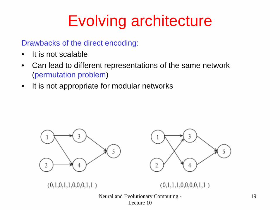
19
Evolving architecture Drawbacks of the direct encoding: • It is not scalable • Can lead to different representations of the same network
(permutation problem) • It is not appropriate for modular networks

Neural and Evolutionary Computing - Lecture 10
20
Evolving architecture Indirect encoding: • Biological motivation • Parametric encoding
– The network is described by a set of characteristics (fingerprint)
– Particular case: feedforward network with variable number of hidden units
– The fingerprint is instantiated in a network only for evaluation • Rules-based encoding

Neural and Evolutionary Computing - Lecture 10
21
Evolving architecture • Parametric encoding
Instantiation: random choice of connections according to the specified characteristics

Neural and Evolutionary Computing - Lecture 10
22
Evolving architecture Example:
Operators: Mutation: change the network
characteristics Recombination: combine characteristics of
layers
Nr. of layers
Param. BP
Info. layer 1
Info. layer 2

Neural and Evolutionary Computing - Lecture 10
23
Evolving architecture Rule-based encoding (similar to Grammar Evolution) :
General rule
Examples:
Structure of an element:

Neural and Evolutionary Computing - Lecture 10
24
Evolving architecture Deriving an architecture:

Neural and Evolutionary Computing - Lecture 10
25
Evolving architecture
Dezavantaj al evoluției separate a arhitecturii: • Ca urmare a antrenării pornind de la valori inițiale aleatoare se
obțin estimări afectate de zgomot al fitness-ului corespunzător unei arhitecturi
Soluții: • Antrenarea de mai multe ori a aceleiași arhitecturi și calculul
fitness-ului mediu => costuri mari • Evoluția simultană a arhitecturii și ponderilor (asigură o
corespondență 1 la 1 a genotipului (codificarea arhitecturii) și a fenotipului (rețeaua antrenată))

Neural and Evolutionary Computing - Lecture 10
26
EPNet Exemplu: EPNet = evolutionary design of feedforward neural networks
using principles of evolutionary proramming [Xin Yao, 1996]
BP
BP+SA
Successful =error decrease
The removed nodes are randomly selected
Successful=better than the worst Network from the population

Neural and Evolutionary Computing - Lecture 10
27
EPNet Network encoding: list of hidden units + Connectivity matrix+ Weight matrix Example: each neuron (except for the first m which are input neurons) is connected to all
previous neurons

Neural and Evolutionary Computing - Lecture 10
28
EPNet Architectures evolved by EPNet for the parity problem
n=7 n=8

Neural and Evolutionary Computing - Lecture 10
29
NEAT NEAT = NeuroEvolution of Augmenting Topologies
(http://nn.cs.utexas.edu/?neat) • Direct encoding:
– List of nodes (neurons) • Type of the nodes: input, hidden, output, bias
– List of connections; for each connection: • In-node • Out-node • Connection weight • Activation bit (0 – active connection, 1- disabled connection) • Innovation value

Neural and Evolutionary Computing - Lecture 10
30
NEAT NEAT = NeuroEvolution of Augmenting Topologies
(http://nn.cs.utexas.edu/?neat)
• The initial population consists of simple architectures (only input and output layers)
• Mutation variants: – Node adding: insert a new node between two already connected
nodes (the old connection is removed and two other connections are added: that entering the new node has the weight=1, that going out from the new node has the weight of the removed connection)
– Connection adding: a new connection (with a random weight) is added between two previously unconnected nodes

Neural and Evolutionary Computing - Lecture 10
31
NEAT Mutation example: (K.Stanley, R. Miikulainen – Evolving Neural
Networks through Augmenting Topologies, Evol.Comput. 2002)

Neural and Evolutionary Computing - Lecture 10
32
NEAT Crossover: 2 parents ---- 1 offspring Similar to uniform crossover used in genetic algorithms Step 1: identify the matching genes from the two parents based on the
innovation values • Two genes match if they have the same innovation value (this
values is assigned when the gene is created) • The non-matching genes are disjoint or in excess genes

Neural and Evolutionary Computing - Lecture 10
33
NEAT Crossover: 2 parents ---- 1 offspring Similar to uniform crossover used in genetic algorithms Step 2: offspring construction • For matching genes the offspring will receive the gene from one of
the parents (randomly selected) • The in excess/disjoint genes are transferred into the ofspring either
based on a probabilistic decision or based on the fitness of the parents (the gene its transferred if it belongs to the better parent)

Neural and Evolutionary Computing - Lecture 10
34
NEAT Crossover example (Stanley,
Miikulainen, 2002)

Neural and Evolutionary Computing - Lecture 10
35
Evolving learning rules General form of a local adjustement rule
),,,,,,),(()1( αδδϕ jijjiiijij yxyxkwkw =+
xi,xj – input signals yi,yj – output signals α – control parameters (ex: learning rate) δi,δj – error signal Example: BackPropagation
jiijij ykwkw ηδ+=+ )()1(

Neural and Evolutionary Computing - Lecture 10
36
Evolving learning rules Elements which can be evolved: • Parameters of the learning process (ex: learning rate, momentum
coefficient) • The adjusting expression (see Genetic Programming)
Evaluation: • Train networks using the corresponding rule Drawback: very high cost

Neural and Evolutionary Computing - Lecture 10
37
Summary General structure Levels: • Weights • Learning rules • Architecture