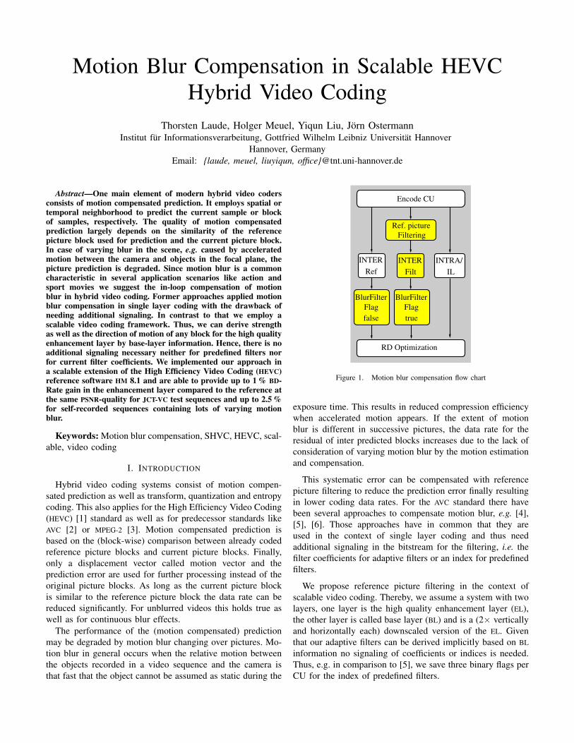
Motion Blur Compensation in Scalable HEVCHybrid Video Coding

Thorsten Laude, Holger Meuel, Yiqun Liu, Jörn OstermannInstitut für Informationsverarbeitung, Gottfried Wilhelm Leibniz Universität Hannover

Hannover, GermanyEmail: {laude, meuel, liuyiqun, office}@tnt.uni-hannover.de

Abstract—One main element of modern hybrid video codersconsists of motion compensated prediction. It employs spatial ortemporal neighborhood to predict the current sample or blockof samples, respectively. The quality of motion compensatedprediction largely depends on the similarity of the referencepicture block used for prediction and the current picture block.In case of varying blur in the scene, e.g. caused by acceleratedmotion between the camera and objects in the focal plane, thepicture prediction is degraded. Since motion blur is a commoncharacteristic in several application scenarios like action andsport movies we suggest the in-loop compensation of motionblur in hybrid video coding. Former approaches applied motionblur compensation in single layer coding with the drawback ofneeding additional signaling. In contrast to that we employ ascalable video coding framework. Thus, we can derive strengthas well as the direction of motion of any block for the high qualityenhancement layer by base-layer information. Hence, there is noadditional signaling necessary neither for predefined filters norfor current filter coefficients. We implemented our approach ina scalable extension of the High Efficiency Video Coding (HEVC)reference software HM 8.1 and are able to provide up to 1 % BD-Rate gain in the enhancement layer compared to the reference atthe same PSNR-quality for JCT-VC test sequences and up to 2.5 %for self-recorded sequences containing lots of varying motionblur.

Keywords: Motion blur compensation, SHVC, HEVC, scal-able, video coding

I. INTRODUCTION

Hybrid video coding systems consist of motion compen-sated prediction as well as transform, quantization and entropycoding. This also applies for the High Efficiency Video Coding(HEVC) [1] standard as well as for predecessor standards likeAVC [2] or MPEG-2 [3]. Motion compensated prediction isbased on the (block-wise) comparison between already codedreference picture blocks and current picture blocks. Finally,only a displacement vector called motion vector and theprediction error are used for further processing instead of theoriginal picture blocks. As long as the current picture blockis similar to the reference picture block the data rate can bereduced significantly. For unblurred videos this holds true aswell as for continuous blur effects.

The performance of the (motion compensated) predictionmay be degraded by motion blur changing over pictures. Mo-tion blur in general occurs when the relative motion betweenthe objects recorded in a video sequence and the camera isthat fast that the object cannot be assumed as static during the

INTRA/

IL

INTER

Ref

BlurFilter

Flag

false

INTER

Filt

BlurFilter

true

Flag

Ref. picture

Filtering

RD Optimization

Encode CU

Figure 1. Motion blur compensation flow chart

exposure time. This results in reduced compression efficiencywhen accelerated motion appears. If the extent of motionblur is different in successive pictures, the data rate for theresidual of inter predicted blocks increases due to the lack ofconsideration of varying motion blur by the motion estimationand compensation.

This systematic error can be compensated with referencepicture filtering to reduce the prediction error finally resultingin lower coding data rates. For the AVC standard there havebeen several approaches to compensate motion blur, e.g. [4],[5], [6]. Those approaches have in common that they areused in the context of single layer coding and thus needadditional signaling in the bitstream for the filtering, i.e. thefilter coefficients for adaptive filters or an index for predefinedfilters.

We propose reference picture filtering in the context ofscalable video coding. Thereby, we assume a system with twolayers, one layer is the high quality enhancement layer (EL),the other layer is called base layer (BL) and is a (2× verticallyand horizontally each) downscaled version of the EL. Giventhat our adaptive filters can be derived implicitly based on BLinformation no signaling of coefficients or indices is needed.Thus, e.g. in comparison to [5], we save three binary flags perCU for the index of predefined filters.

II. REFERENCE PICTURE FILTERING

Since motion blur changing over time largely degrades thequality of the picture prediction process we suggest to filter theEL reference picture in order to increase the similarity betweenthese reference pictures and the current picture. Therefore anadjustment of the motion blur extend is applied. The BL doesnot need a motion blur compensation itself, as motion blurprimary appears in high frequency components not present inBL due to downsampling and higher quantization parameters(QPs). However, we employ BL information to derive appropri-ate filter coefficients assuming the differences are caused bychanging motion blur.

Based upon the motion vector (MV) of the co-locatedBL coding unit (CU) a two-dimensional directional filter isderived and applied to the EL reference pictures. For thisderivation we use two different low-pass filters as base, onefor the luminance and one for the chrominance signal with thefilter coefficients set according to Table I. The correspondingfrequency responses are shown in Fig. 2.

Table IFILTER COEFFICIENTS

Base filter for CoefficientsLuma with direction 1 1 1 2 1 1 1

Luma without direction

[1 2 12 4 21 2 1

]Chroma 1 2 1

Since these filters have only one coefficient unequal to “1”each, a computational efficient implementation with additionsand only one multiplication is possible. The normalization ofthe filter result is realized using bit shifts.

If the MV of the co-located BL CU is available and at leastone MV component is unequal to zero, the angle of the MVtowards the positive horizontal axis is calculated and quantizedto the nearest element of {0◦, 45◦, 90◦, 135◦, 180◦, 225◦,270◦, 315◦}. This way the possible directions of the two-dimensional filter are restricted to eight: the horizontal andvertical directions and the directions on the diagonals. Usingthis approach we are able to design 2D filters with very fewcoefficients by placing the coefficients of a 1D base filter onthese directions while the rest of the 2D filter’s coefficientsremain zero as illustrated below in (1).

[1 2 1

]and ↖ ⇒

1 0 00 2 00 0 1

(1)

In cases where the co-located BL CU has no MV, i.e. the CUis intra or inter-layer (IL) predicted, or both MV componentsare equal to zero we tested a 2D non-directional boxfilter.

The motion blur compensation is designed as locally adap-tive approach. Consequently, the filter design and the decisionprocess whether to use this method or not within the rate-distortion (RD) process are applied on (sub-)CU level.

Figure 1 shows the process of encoding a CU. We added oneadditional path to the encoder. In addition to the already ex-

0 0.2 0.4 0.6 0.8 10

0.2

0.4

0.6

0.8

1

Frequency [π]

Filt

er r

espo

nse

Filter lumaFilter chroma

Figure 2. Basefilter frequency responses

isting coding modes (Inter/Intra/IL prediction) inter predictionwith a filtered reference picture is tested. Within the encodingprocess we added one binary “BlurFilter Flag” per CU to signalto the decoder if the reference picture block has to be filteredfor proper reconstruction of the current picture block or not.However, this flag is only coded for those CUs for which themotion blur compensation is relevant (i.e. inter predicted CUs).This flag is also included in the RD optimization.

III. EXPERIMENTS

For our simulations we implemented our algorithm in theJCT-VC K0345 [7] software which is a scalable extension of theHEVC reference software HM 8.1.

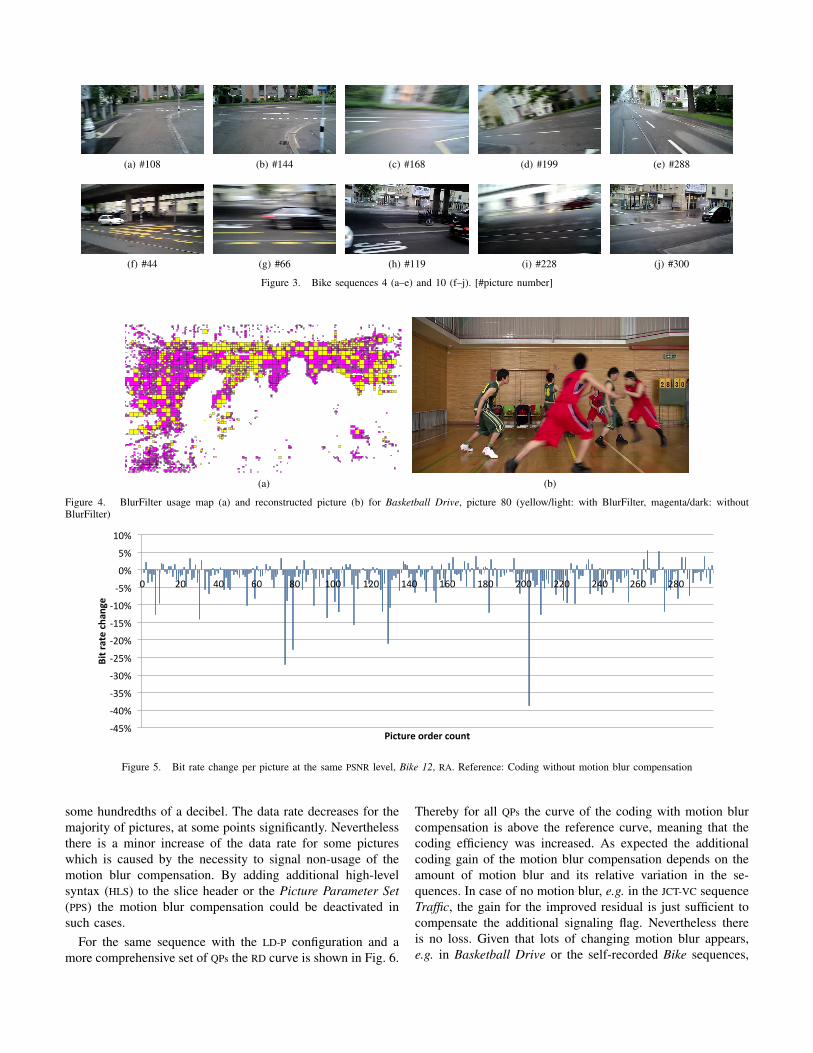
The evaluation of the proposed approach is based on theJCT-VC common test conditions [8] using a 2× scalability, theRandom Access (RA) and Low Delay (LD-P) configuration andan extended set of test sequences. The latter contains JCT-VC test sequences (Basketball Drive, China Speed, Kimono,Tennis, Traffic) as well as self-recorded test sequences withlots of (varying) motion blur. Our self-recorded sequences(1280 × 720, 30 fps, 300 pictures each) were filmed with acamera attached to a bike driver’s helmet. This camera has afixed focal length. Hence, no blur is introduced by alteringthe focus. In the following we refer to these sequences asBike sequences. Due to camera shake and the driver lookingaround to capture the traffic situation these sequences showlots of accelerated motions. The sequence characteristics aredemonstrated in Fig. 3.

The usage of the motion blur compensation is illustratedwith a usage map next to the reconstructed picture in Fig. 4.For the colored CUs, which are the inter predicted CUs forwhom the BlurFilter is potentially applied, the color indicateswhether our method has been chosen (yellow/light) by the RD-process or not (magenta/dark). Besides, it is noteworthy thatthe players’ complex motion can be better described with ILtexture prediction than with motion compensated predictionboth with or without motion blur compensation.

For the sequence Bike 12 the bit rate change per picture isanalyzed according to Fig. 5. Thereby a negative change indi-cates a better compression since the PSNR difference betweenthe coding with and without BlurFilter is at the maximum

(a) #108 (b) #144 (c) #168 (d) #199 (e) #288

(f) #44 (g) #66 (h) #119 (i) #228 (j) #300

Figure 3. Bike sequences 4 (a–e) and 10 (f–j). [#picture number]

0 200 400 600 800 1000 1200 1400 1600 1800 2000

0

200

400

600

800

1000

1200(a) (b)

Figure 4. BlurFilter usage map (a) and reconstructed picture (b) for Basketball Drive, picture 80 (yellow/light: with BlurFilter, magenta/dark: withoutBlurFilter) Plot

Seite 1

-­‐45%  

-­‐40%  

-­‐35%  

-­‐30%  

-­‐25%  

-­‐20%  

-­‐15%  

-­‐10%  

-­‐5%  

0%  

5%  

10%  

0   20   40   60   80   100   120   140   160   180   200   220   240   260   280  

Bit  rate  chan

ge  

Picture  order  count  

Figure 5. Bit rate change per picture at the same PSNR level, Bike 12, RA. Reference: Coding without motion blur compensation

some hundredths of a decibel. The data rate decreases for themajority of pictures, at some points significantly. Neverthelessthere is a minor increase of the data rate for some pictureswhich is caused by the necessity to signal non-usage of themotion blur compensation. By adding additional high-levelsyntax (HLS) to the slice header or the Picture Parameter Set(PPS) the motion blur compensation could be deactivated insuch cases.

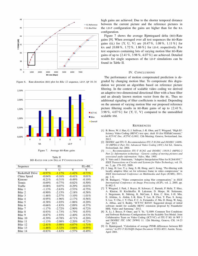
For the same sequence with the LD-P configuration and amore comprehensive set of QPs the RD curve is shown in Fig. 6.

Thereby for all QPs the curve of the coding with motion blurcompensation is above the reference curve, meaning that thecoding efficiency was increased. As expected the additionalcoding gain of the motion blur compensation depends on theamount of motion blur and its relative variation in the se-quences. In case of no motion blur, e.g. in the JCT-VC sequenceTraffic, the gain for the improved residual is just sufficient tocompensate the additional signaling flag. Nevertheless thereis no loss. Given that lots of changing motion blur appears,e.g. in Basketball Drive or the self-recorded Bike sequences,

36  

38  

40  

42  

44  

46  

48  

0   1000   2000   3000   4000   5000   6000   7000  

Y  PSNR  [dB]  

Bit  rate  [kbps]  

EL  Reference  

EL  BlurFilter  

Figure 6. Rate-distortion (RD) plot for Bike 12 sequence, LD-P, QP 18–34

0,00%  

0,50%  

1,00%  

1,50%  

2,00%  

2,50%  

Y   U   V   Y   U   V  

RA     LD-­‐P  

JCT-­‐VC  

Bike  

Overall  

Figure 7. Average BD-Rate gains

Table IIBD-RATES FOR LOW DELAY P CONFIGURATION

Sequence EL EL+BLY U V Y

Basketball Drive -0.97% -1.17% -1.42% -0.73%China Speed -0.04% -0.16% -0.41% 0.01%Kimono -0.21% -0.31% -0.49% -0.10%Tennis -0.69% -0.77% -0.82% -0.50%Traffic -0.08% 0.07% -0.29% -0.03%Bike 1 -1.13% -2.63% -2.53% -0.75%Bike 2 -0.90% -2.15% -2.18% -0.58%Bike 3 -1.46% -2.57% -3.10% -1.01%Bike 4 -0.95% -1.96% -2.17% -0.56%Bike 5 -0.38% -1.03% -1.06% -0.20%Bike 6 -0.66% -1.83% -2.09% -0.37%Bike 7 -1.17% -2.72% -2.90% -0.72%Bike 8 -0.93% -1.73% -1.79% -0.55%Bike 9 -0.87% -1.93% -2.40% -0.53%Bike 10 -0.39% -0.78% -0.71% -0.20%Bike 11 -1.13% -2.08% -2.20% -0.72%Bike 12 -2.41% -3.98% -4.07% -1.71%Bike 13 -1.46% -3.32% -3.04% -0.95%Bike 14 -0.83% -1.63% -1.57% -0.49%

high gains are achieved. Due to the shorter temporal distancebetween the current picture and the reference pictures inthe LD-P configuration the gains are higher than for the RAconfiguration.

Figure 7 shows the average Bjøntegaard delta (BD)-Rategains [9]. When averaged over all test sequences the BD-Rategains (EL) for {Y, U, V} are {0.47 %, 1.08 %, 1.11 %} forRA and {0.88 %, 1.72 %, 1.86 %} for LD-P, respectively. Fortest sequences containing lots of varying motion blur BD-Rategains of up to {2.41 %, 3.98 %, 4.07 %} are achieved. Detailedresults for single sequences of the LD-P simulations can befound in Table II.

IV. CONCLUSIONS

The performance of motion compensated prediction is de-graded by changing motion blur. To compensate this degra-dation we present an algorithm based on reference picturefiltering. In the context of scalable video coding we derivedan adaptive two-dimensional directional filter with a base filterand an already known motion vector from the BL. Thus noadditional signaling of filter coefficients is needed. Dependingon the amount of varying motion blur our proposed referencepicture filtering results in BD-Rate gains of up to {2.41 %,3.98 %, 4.07 %} for {Y, U, V} compared to the unmodifiedscalable HM.

REFERENCES

[1] B. Bross, W.-J. Han, G. J. Sullivan, J.-R. Ohm, and T. Wiegand, “High Ef-ficiency Video Coding (HEVC) text spec. draft 10 (for FDIS&Consent),”in JCT-VC Doc. JCTVC-L1003, 12th Meeting: Geneva, Switzerland, Jan.2013.

[2] ISO/IEC and ITU-T, Recommendation ITU-T H.264 and ISO/IEC 14496-10 (MPEG-4 Part 10): Advanced Video Coding (AVC)-3rd Ed., Geneva,Switzerland, Jul. 2004.

[3] ——, Recommendation ITU-T H.262 and ISO/IEC 13818-2 (MPEG-2Part 2): Information technology - Generic coding of moving pictures andassociated audio information: Video, Mar. 1995.

[4] Y. Vatis and J. Ostermann, “Adaptive Interpolation Filter for H.264/AVC,”IEEE Transactions on Circuits and Systems for Video Technology, vol. 19,no. 2, pp. 179–192, 2009.

[5] J. Jang, H. Lee, T.-y. Jung, S.-M. Hong, and J. Jeong, “Pre-filtering withlocally adaptive filter set for reference frame in video compression,” inIEEE International Conference on Multimedia and Expo (ICME), 2011,pp. 1–6.

[6] M. Budagavi, “Video compression using blur compensation,” in IEEEInternational Conference on Image Processing (ICIP), vol. 2, 2005, pp.II–882–5.

[7] T. Wiegand, J. Park, J. Boyce, H. Schwarz, C. Bartnik, P. Helle, T. Hinz,A. Khairat, H. Kirchhoffer, H. Laksman, D. Marpe, M. Siekmann,J. Stegemann, K. Sühring, K. McCann, J. Kim, C. Kim, J.-H. Min,E. Alshina, A. Alshin, I.-K. Kim, T. Lee, B. Choi, Y. Piao, S. Jeong,S. Lee, Y. Cho, J. Y. Choi, F. C. A. Fernandes, Z. Ma, D. Hong, W. Jang,A. Abbas, and S. Reddy, “JCT-VC K0345: Suggested design of initialsoftware model for scalable HEVC extension proposal by FraunhoferHHI, Vidyo and Samsung,” 2012.

[8] X. Li, J. Boyce, P. Onno, and Y. Ye, “L1009: Common Test Conditionsand Software Reference Configurations for the Scalable Test Model. JointCollaborative Team on Video Coding (JCT-VC) of ITU-T SG 16 WP 3and ISO/IEC JTC 1/SC 29/WG 11. 12th Meeting, Geneva, CH, 14-23Jan,” 2013.

[9] G. Bjøntegaard, “Calculation of average PSNR differences between RDcurves,” in ITU-T SG16/Q6 Output Document VCEG-M33, Austin, Texas,April 2001.