MOSTAFA ABOBAKER - uvidok.rcub.bg.ac.rs
230
UNIVERSITY OF BELGRADE FACULTY OF MECHANICAL ENGINEERING MOSTAFA ABOBAKER LOW REYNOLDS NUMBER AIRFOILS DOCTORAL DISSERTATION BELGRADE 2017
Transcript of MOSTAFA ABOBAKER - uvidok.rcub.bg.ac.rs

UNIVERSITY OF BELGRADE
FACULTY OF MECHANICAL ENGINEERING
MOSTAFA ABOBAKER
LOW REYNOLDS NUMBER AIRFOILS
DOCTORAL DISSERTATION
BELGRADE 2017

УНИВЕРЗИТЕТ У БЕОГРАДУ
МАШИНСКИ ФАКУЛТЕТ
Мосtафа Абобакер
АЕРОПРОФИЛИ ЗА МАЛЕ РЕЈНОЛДСОВЕ
БРОЈЕВЕ
Докторска дисертација
БЕОГРАД, 2017

TO MY FAMILY

ACKNOWLEDGEMENTS
I would like to express my sincere thanks and gratitude to my advisor professor Zlatko
Petrovic for his valuable and continuous advice, thoughtfulness and assistance throughout the
duration of this work.
I would like to express my sincere thanks and gratitude to all PhD program staff members in
Mechanical Engineering Faculty and to the Innovation Center in Mechanical Engineering
Faculty.
I would like to express my gratitude to Libyan Ministry of High Education and Science
Research and to Libyan Scholarship Administration for their financial support. This research
would not have been accomplished without their support.
I also would like to take this opportunity to thank my family who are surely proud of me on
this day.
Special thanks to the staffs, students and friends that I have met during my research study
especially those in the Mechanical Engineering Department.
Above all, I am very much grateful to almighty Allah for giving me courage and good health
for completing this research.
Mostafa Abobaker
BELGRADE 2017
i
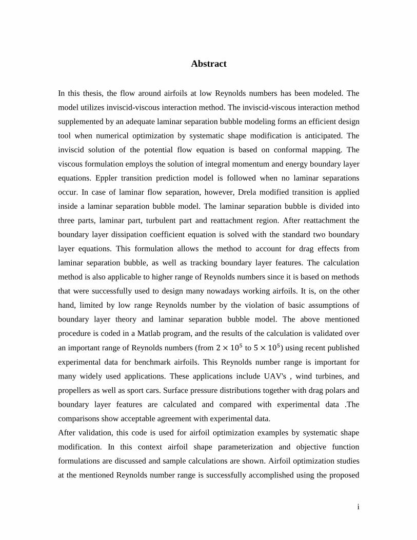
Abstract
In this thesis, the flow around airfoils at low Reynolds numbers has been modeled. The
model utilizes inviscid-viscous interaction method. The inviscid-viscous interaction method
supplemented by an adequate laminar separation bubble modeling forms an efficient design
tool when numerical optimization by systematic shape modification is anticipated. The
inviscid solution of the potential flow equation is based on conformal mapping. The
viscous formulation employs the solution of integral momentum and energy boundary layer
equations. Eppler transition prediction model is followed when no laminar separations
occur. In case of laminar flow separation, however, Drela modified transition is applied
inside a laminar separation bubble model. The laminar separation bubble is divided into
three parts, laminar part, turbulent part and reattachment region. After reattachment the
boundary layer dissipation coefficient equation is solved with the standard two boundary
layer equations. This formulation allows the method to account for drag effects from
laminar separation bubble, as well as tracking boundary layer features. The calculation
method is also applicable to higher range of Reynolds numbers since it is based on methods
that were successfully used to design many nowadays working airfoils. It is, on the other
hand, limited by low range Reynolds number by the violation of basic assumptions of
boundary layer theory and laminar separation bubble model. The above mentioned
procedure is coded in a Matlab program, and the results of the calculation is validated over
an important range of Reynolds numbers (from to ) using recent published
experimental data for benchmark airfoils. This Reynolds number range is important for
many widely used applications. These applications include UAV's , wind turbines, and
propellers as well as sport cars. Surface pressure distributions together with drag polars and
boundary layer features are calculated and compared with experimental data .The
comparisons show acceptable agreement with experimental data.
After validation, this code is used for airfoil optimization examples by systematic shape
modification. In this context airfoil shape parameterization and objective function
formulations are discussed and sample calculations are shown. Airfoil optimization studies
at the mentioned Reynolds number range is successfully accomplished using the proposed

ii
code and methodology. Airfoil shape design is efficiently achieved by systematic shape
modification and direct aerodynamic calculation.
Key words: Airfoils, low Reynolds number, conformal mapping, airfoil
aerodynamics, airfoil shape parameterization, aerodynamic
optimization.
Scientific discipline: Aeronautical Engineering
Scientific sub-discipline: Aerodynamics
UDC:

iii
АПСТРАКТ
У овој тези је моделирано струјање око аеропрофила са ниским Рејнолдсовим бројем.
Вискозно невискозна интеракција комбинована са моделирањем ламинарног мехура
је ефикасан метод за конструисање нових аеропрофила систематским
модификовањем облика аеропрофила. Невискозно решење је засновано на
конформном пресликавању. Вискозна формулација је заснована на решавању
интегралних једначина за количину кретања и енергије. Када нема одцепљења
струјања примењен је Еплеров модел за предвиђање транзиције из ламинарног у
турбулентно струјање. Ламинарни мехур, који узрокује отцепљење је моделиран из
три сегмента: ламинарни део, турбулентни део и област прилепљења струјања.
Овиме је омогућено одређивање доприноса укупном отпору аеропрофила, такође је
омогућено и праћење карактеристика граничног слоја.
Прорачунски метод је применљив и за конструисање аеропрофила за лет при вишим
Рејнолдсовим бројевима јер је базиран на методима који су превиђени за такво
конструисање. Метод је програмиран помоћу MATLAB-a за област Рејнолдосивих
бројева (од до ) решења су поређена са експерименталним
резултатима. Одабрана област Рејнолдсових бројева има веома велики праткчни
значај. Конструисани аеропрофили су примењиви код беспилотних летелица,
лопатица ветротурбина, лопатица пропелера, као и код узгонских аеропрофила на
аутомобилима.
Прорачунате су расподеле притисака, поларе, и карактеристике граничног слоја и
упоређене са расположивим експерименталним подацима. Поређење показује
задовољавајуће слагање између прорачуна и експерименталних података.
Након верификације прорачуном је одређено више оптималних аеропрофила за
различите услове. Аеропрофил је параметризован на неколико опционих начина, а
функција циља за оптимизацију је дефинисана такође на више начина.
Продискутовани су различити оптимизациони критеријуми и за њих је одређен

iv
оптимални облик аеропрофила. Развијени софтвер омогућује ефикасно пројектовање
нових облика аеропрофила са систематском модификацијом облика аеропрофила.
Key words: Aeroprofili, mali Rejnoldsovi brojevi, konformno
preslikavanje, aerodinamika aeroprofila, parametrizacija
oblika aeroprofila, aerodinamicka optimizacija
Scientific discipline: Vazduhoplovstvo
Scientific sub-discipline: Aerodinamika
UDC:

v
Table of Contents
Table of Contents ABSTRACT ........................................................................................................................ I TABLE OF FIGURES ................................................................................................. VIII NOMENCLATURE ................................................................................................... XVII CHAPTER 1 ...................................................................................................................... 1
1 INTRODUCTION ........................................................................................................ 1 1.1 LOW REYNOLDS NUMBER AIRFOILS ...................................................................... 3 1.2 EFFICIENCY IN AIRFOIL DESIGN ............................................................................. 5 1.3 THESIS OUTLINE ................................................................................................... 6
CHAPTER 2 ...................................................................................................................... 8 2 TWO DIMENSIONAL IDEAL FLUID FLOW ........................................................ 8
2.1 ASSUMPTION OF AN IDEAL FLUID [12] .................................................................. 9
2.2 FUNDAMENTAL PRINCIPLES ................................................................................ 10 2.2.1 Irrotational flow ......................................................................................... 10 2.2.2 Velocity Potential and stream function ..................................................... 11
2.2.3 The complex Velocity ............................................................................... 12
2.2.4 The Complex Potential .............................................................................. 13 2.2.5 Circular Cylinder with Circulation ............................................................ 16 2.3 APPLICATION TO AIRFOILS AND CONFORMAL TRANSFORMATIONS ...................... 18
2.4 KARMA-TREFFTZ TRANSFORMATION .................................................................. 21 2.5 FLOW ANALYSIS OVER AN AIRFOIL USING CONFORMAL MAPPING .................... 22
2.5.1 Airfoil shape .............................................................................................. 24 2.5.2 Apply Karman-Trefftz Transformation ..................................................... 25 2.5.3 Translation of the near circle to the origin ................................................ 26
2.5.4 Mapping of near circle in plane) to true circle ( plane). .................. 27 2.5.5 Calculation of modulus of transformation ................................................. 30
2.5.6 Finding velocities in the true circle plane .................................................. 32
CHAPTER 3 .................................................................................................................... 37 3 BOUNDARY LAYER MODELING ........................................................................ 37
3.1 BOUNDARY LAYER CONCEPT ............................................................................. 37 3.2 BOUNDARY LAYER SEPARATION ......................................................................... 39
3.3 SHEAR STRESS AND FRICTION DRAG ................................................................... 41 3.4 BOUNDARY LAYER MOMENTUM AND ENERGY INTEGRAL EQUATIONS ................. 42 3.4.1 Boundary layer integral approach.............................................................. 44 3.4.2 Laminar boundary layer............................................................................. 45 3.4.3 Turbulent boundary layer .......................................................................... 47
3.5 BOUNDARY LAYER TRANSITION .......................................................................... 48 3.6 LAMINAR SEPARATION BUBBLE .......................................................................... 50
3.7 EPPLER’S BUBBLE PREDICTION METHOD ............................................................ 52 3.8 LIFT, DRAG AND MOMENT ................................................................................... 52

vi
3.8.1 Integration of pressure and shear stress distributions ................................ 54 3.8.2 Lift Drag Moment corrections ................................................................... 55 3.9 COMPARISON OF TURBULENT CLOSURE RELATIONS ............................................ 56 3.9.1 Eppler turbulent model: ............................................................................. 57 3.9.2 Drela Turbulent closure ............................................................................. 57
3.9.3 Modified Drela model used by LUTZ and Wagner [38] ........................... 59 3.9.4 Lutz and Wagner model ............................................................................ 59 3.10 VERIFICATION OF BOUNDARY LAYER CALCULATIONS ........................................ 63 3.10.1 Comparison with Eppler code ................................................................... 63
3.10.2 Comparisons with XFOIL code ................................................................. 69
CHAPTER 4 .................................................................................................................... 72 4 LAMINAR SEPARATION BUBBLE MODELING ............................................... 72
4.1 REYNOLDS NUMBER AND ANGLE OF ATTACK VARIATION ................................... 76 4.2 LAMINAR SEPARATION BUBBLE MODEL .............................................................. 78 4.2.1 Laminar part of the bubble [36] ................................................................. 79 4.2.2 Transition ................................................................................................... 82
4.2.3 Turbulent part of the bubble ...................................................................... 83 4.2.4 Intersection with inviscid distribution ....................................................... 88 4.2.5 Attached turbulent boundary layer ............................................................ 88
4.3 VALIDATION OF AERODYNAMIC CALCULATIONS ................................................ 91
4.3.2 Variation of aerodynamic coefficients with Reynolds number ............... 102 4.3.3 Variation of boundary layer features with Reynolds number.................. 105
CHAPTER 5 .................................................................................................................. 109 5 AIRFOIL PARAMETRIC REPRESENTATION................................................. 109
5.1 GENERAL REQUIREMENT .................................................................................. 109
5.2 NACA AIRFOIL SERIES .................................................................................... 110 5.3 4-DIGIT SERIES AIRFOILS ................................................................................... 110 5.4 PARSEC METHOD ........................................................................................... 113
5.5 BEZIER PARAMETERIZATION ............................................................................ 117 5.6 CST METHOD ................................................................................................... 121
5.7 MATCHING OF NACA 4412 AIRFOIL SHAPE ..................................................... 127
5.8 MATCHING OF TARGET PRESSURE DISTRIBUTION ............................................ 132 5.8.1 CST with n=2 parameters ........................................................................ 133 5.8.2 CST with n=4 parameters ........................................................................ 135
CHAPTER 6 .................................................................................................................. 138 6 AERODYNAMIC DESIGN AND SHAPE OPTIMIZATION ............................. 138
6.1 INVERSE DESIGN APPROACH ............................................................................. 139 6.2 DIRECT DESIGN APPROACH ............................................................................... 140 6.3 NUMERICAL OPTIMIZATION .............................................................................. 141 6.3.1 Formulation of the mathematical problem .............................................. 142
6.3.2 Genetic Search algorithms ....................................................................... 142 6.3.3 Choice of constraints ............................................................................... 144 6.3.4 Formulation of objective function ........................................................... 144
6.3.5 Single objective versus multi objective optimization .............................. 145 6.4 DIRECT AERODYNAMIC OPTIMIZATION BY SHAPE PERTURBATION .................... 146

vii
CHAPTER 7 .................................................................................................................. 149 7 AIRFOIL OPTIMIZATION CASE STUDIES ..................................................... 149
7.1 PROBLEM FORMULATION .................................................................................. 152 7.2 GEOMETRIC CONSTRAINTS: .............................................................................. 153 7.3 AIRFOIL PARAMETERIZATION ........................................................................... 153
7.4 FORMULATION OF THE OBJECTIVE FUNCTION ................................................... 154 7.4.1 Equality and Inequality Constrained Optimization and Penalty Function154 7.5 DESIGN FOR GIVEN PRESSURE DISTRIBUTION (INVERSE DESIGN) ...................... 157 7.5.1 NACA 0012 ............................................................................................. 157
7.5.2 LIEBECK LNV109A high lift airfoil ...................................................... 162 7.6 SINGLE POINT SINGLE OBJECTIVE ...................................................................... 165 7.6.1 Aerodynamic constraints ......................................................................... 165
7.6.2 Optimization Results ............................................................................... 165 7.6.3 Airfoil shape and pressure distributions .................................................. 167 7.6.4 Aerodynamic coefficients ........................................................................ 169 7.7 SINGLE POINT MULTI OBJECTIVE ....................................................................... 170
7.7.1 Optimization Results ............................................................................... 171 7.7.2 Airfoil shape and pressure distributions .................................................. 173 7.7.3 Aerodynamic coefficients ........................................................................ 174
7.8 MULTI POINT SINGLE OBJECTIVE ....................................................................... 176
7.8.1 Aerodynamic constraints ......................................................................... 176 7.8.2 Optimization Results ............................................................................... 176 7.8.3 Airfoil shape and pressure distributions .................................................. 177
7.8.4 Lift and drag polar ................................................................................... 179 7.9 MULTI POINT MULTI OBJECTIVE ...................................................................... 180
7.9.1 Drag minimization at a range of operating lift coefficients..................... 180 7.9.2 Objective function formulation ............................................................... 180 7.9.3 Optimization Results ............................................................................... 181
7.9.4 Airfoil shape and pressure distributions .................................................. 182 7.9.5 Lift and drag polar ................................................................................... 184
7.10 DESIGN AT DIFFERENT REYNOLDS NUMBERS .................................................... 186
7.10.1 Optimization at different Reynolds numbers........................................... 189
8 CONCLUSION ......................................................................................................... 194 8.1 AERODYNAMIC ANALYSIS ................................................................................ 194 8.2 AIRFOIL PARAMETERIZATION ........................................................................... 196 8.3 OBJECTIVE FUNCTION AND CONSTRAINTS ......................................................... 196
8.4 AIRFOIL DESIGN AND OPTIMIZATION ................................................................. 197 8.5 FUTURE WORK .................................................................................................. 199
9 REFERENCES ......................................................................................................... 200

viii
Table of Figures
FIGURE 1.1 THE CODE FLOW CHART .......................................................................... 2
FIGURE 1.2 CHORD REYNOLDS NUMBER VS. FLIGHT SPEED FOR
DIFFERENT NATURAL AND MANMADE OBJECTS ........................... 4
FIGURE 1.3 REYNOLDS NUMBER EFFECT ON REPRESENTATIVE AIRFOILS
PERFORMANCE .......................................................................................... 5
FIGURE 2.1 HIERARCHY OF THE DIFFERENT LEVELS OF APPROXIMATION
[12] ................................................................................................................. 9
FIGURE 2.2 CIRCULATION AROUND CLOSED PATH [13] ...................................... 11
FIGURE 2.3 VARIABLES DEFINING COMPLEX VELOCITY .................................... 13
FIGURE 2.4 A TYPICAL STREAM LINES OF FLOW AROUND CIRCULAR
CYLINDER WITH MODERATE CIRCULATION Γ ............................... 16
FIGURE 2.5 (A) A UNIT CIRCLE IN Z PLANE CENTERED AT ORIGIN WITH
UNIT RADIUS. (B) JOUKOWSKY TRANSFORM OF Z PLANE
UNIT CIRCLE TO A STRAIGHT LINE SEGMENT FROM -2 TO 2
IN PLANE. ............................................................................................... 20
FIGURE 2.6 (A) A CIRCLE CENTERED AT ORIGIN WITH RADIUS DIFFERENT
THAN 1 IN Z PLANE TRANSFORMED INTO ELLIPSE IN
PLANE. ........................................................................................................ 20
FIGURE 2.7 CLOSE UP OF TRAILING EDGE REGIONS SHOWING ZERO
TRAILING EDGE ANGLE. ....................................................................... 20
FIGURE 2.8 (A) A CIRCLE CENTERED OFF THE ORIGIN AND HAS TOUCHES
THE UNIT CIRCLE AT ONE POINT . (B) TRANSFORMED INTO
AN ELLIPSE WHICH TOUCHES MID-REAL AXIS IN PLANE AT
ONE POINT................................................................................................. 21
FIGURE 2.9 (A) A UNIT CIRCLE WITH CENTER OFFSET ON REAL X AXIS IN
PLANE (B) A NON CAMBERED AIRFOIL IN PLANE. .................. 21
FIGURE 2.10 (A) CIRCLE WITH CENTER OFF THE ORIGIN IN BOTH
AND .WITH PART OF THE CONTOUR OUTSIDE THE
UNIT CIRCLE (B) CAMBERED AIRFOIL IN PLANE WITH
PART OF ITS CONTOUR ABOVE REAL AXIS. .................................... 21
FIGURE 2.11 KARMAN-TREFFTZ TRANSFORM OF AN OFF CENTERED UNIT
CIRCLE WITH AND AND RADIUS OF
1.0512 IN PLANE INTO AN AIRFOIL, WITH FINITE TRAILING
EDGE ANGLE OF 2 DEG IN PLANE. ................................................... 22

ix
FIGURE 2.12 STEPS INVOLVED IN TRANSFORMATIONS OF AIRFOIL TO
TRUE CIRCLE ............................................................................................ 24
FIGURE 2.13 AIRFOIL GENERATED FOR CONFORMAL MAPPING ....................... 25
FIGURE 2.14 AIRFOIL TRANSFORMED TO NEAR CIRCLE ...................................... 26
FIGURE 2.15 SHIFTED NEAR CIRCLE .......................................................................... 27
FIGURE 2.16 NACA4412 AIRFOIL TRANSFORMED TO NEAR CIRCLE THEN
SHIFTED TO ORIGIN ................................................................................ 27
FIGURE 2.17 POTENTIAL FLOW VELOCITY AROUND CIRCULAR CYLINDER
DW/DZ ........................................................................................................ 34
FIGURE 2.18 DERIVATIVE OF TRANSFORMATION (DΖ2/DZ ) FOR E387
AIRFOIL. ..................................................................................................... 34
FIGURE 2.19 DERIVATIVE OF TRANSFORMATION DZ1/Σ FOR E387 AIRFOIL ... 35
FIGURE 2.20 INVISCID PRESSURE DISTRIBUTIONS AT 2O AND REYNOLDS
NUMBER OF 300,000 FOR E387 AIRFOIL. ............................................ 35
FIGURE 2.21 FLOW CHART FOR THE METHOD OF CALCULATION ..................... 36
FIGURE 3.1 BOUNDARY LAYER CONCEPT ............................................................... 38
FIGURE 3.2 SEPARATION OF BOUNDARY LAYER, DEFINED WHEN THE
SLOPE OF THE VELOCITY GRADIENT AT THE WALL IN THE
NORMAL DIRECTION EQUALS ZERO. ................................................ 39
FIGURE 3.3 VELOCITY DISTRIBUTION IN BOUNDARY LAYER AT
DIFFERENT PRESSURE SITUATIONS ................................................... 40
FIGURE 3.4 BOUNDARY LAYER EFFECTS ................................................................. 41
FIGURE 3.5 VISCOUS DRAG COMPUTATION FROM SHEAR STRESS .................. 42
FIGURE 3.6 EPPLER TRANSITION CRITERIA FOR DIFFERENT ROUGHNESS
FACTOR VALUES ..................................................................................... 49
FIGURE 3.7 SKETCH OF LAMINAR SEPARATION BUBBLE .................................... 50
FIGURE 3.8 EFFECT OF SEPARATION BUBBLE ON VELOCITY
DISTRIBUTION.......................................................................................... 51
FIGURE 3.9 EPPLER'S BUBBLE ANALOGY ................................................................. 52
FIGURE 3.10 SIGN CONVENTIONS FOR PRESSURE AND SHEAR STRESS .......... 53
FIGURE 3.11 BODY AND WIND AXIS SYSTEMS ....................................................... 53
FIGURE 3.12 LIFT AND MOMENT CORRECTIONS DUE TO BOUNDARY
LAYER SEPARATION .............................................................................. 56
FIGURE 3.13 COMPARISONS OF DIFFERENT SHAPE FACTOR RELATIONS
FOR INCOMPRESSIBLE TURBULENT BOUNDARY LAYER AT
............................................................................................... 59
FIGURE 3.14 COMPARISONS OF DIFFERENT SHAPE FACTOR RELATIONS
FOR INCOMPRESSIBLE TURBULENT BOUNDARY LAYER AT
................................................................................................. 60

x
FIGURE 3.15 COMPARISONS OF DIFFERENT SHAPE FACTOR RELATIONS
FOR INCOMPRESSIBLE TURBULENT BOUNDARY LAYER AT
................................................................................................. 60
FIGURE 3.16 COMPARISONS OF DIFFERENT SHAPE FACTOR RELATIONS
FOR INCOMPRESSIBLE TURBULENT BOUNDARY LAYER AT
................................................................................................. 61
FIGURE 3.17 COMPARISONS OF DIFFERENT SHAPE FACTOR RELATIONS
FOR INCOMPRESSIBLE TURBULENT BOUNDARY LAYER AT
................................................................................................. 61
FIGURE 3.18 COMPARISONS OF DIFFERENT SHAPE FACTOR RELATIONS
FOR INCOMPRESSIBLE TURBULENT BOUNDARY LAYER,
FROM REFERENCE [38] ........................................................................... 62
FIGURE 3.19 EPPLER AIRFOIL E1098 AND VELOCITY DISTRIBUTION AT RE
1E06 AND ....................................................................................... 63
FIGURE 3.20 COMPARISON OF DRAG COEFFICIENT FOR E1098 AT
BETWEEN CURRENT CALCULATION AND EPPLER CODE. ........... 64
FIGURE 3.21 COMPARISON OF LOCATION OF UPPER SURFACE
TRANSITION POINT FOR E1098 AT BETWEEN
CURRENT CALCULATION AND EPPLER CODE. ............................... 65
FIGURE 3.22 COMPARISONS OVER E1098 AIRFOIL UPPER SURFACE AT
RE 1E06 , .......................................................................................... 65
FIGURE 3.23 COMPARISONS OVER E1098 AIRFOIL LOWER SURFACE
AT RE 1E06 , .................................................................................... 66
FIGURE 3.24 COMPARISONS OVER E1098 AIRFOIL UPPER SURFACE AT
RE 1E06 , .......................................................................................... 66
FIGURE 3.25 COMPARISONS OVER E1098 AIRFOIL LOWER SURFACE AT
RE=1E06 , ......................................................................................... 67
FIGURE 3.26 SHAPE FACTOR DEVELOPMENT OVER E1098 AIRFOIL
SURFACES AS CALCULATED ............................................................... 67
FIGURE 3.27 REYNOLDS NUMBER BASED ON OVER THE AIRFOIL
SURFACE.................................................................................................... 68
FIGURE 3.28 REYNOLDS NUMBER BASED ON OVER THE AIRFOIL
SURFACE.................................................................................................... 68
FIGURE 3.29 NACA 4412 AIRFOIL SHAPE AND VELOCITY DISTRIBUTION
USING CURRENT CALCULATION ........................................................ 69
FIGURE 3.30 COMPARISONS OF SHAPE FACTOR , .......................................... 70
FIGURE 3.31 COMPARISONS OF BOUNDARY LAYER THICKNESS ................ 70

xi
FIGURE 3.32 COMPARISONS OF SKIN FRICTION COEFFICIENT ON UPPER
SURFACE .............................................................................................. 71
FIGURE 4.1 CHORD REYNOLDS NUMBER VS. FLIGHT SPEED FOR
DIFFERENT NATURAL AND MANMADE OBJECTS ......................... 73
FIGURE 4.2 A SCHEMATIC SHAPE OF SHORT LAMINAR SEPARATION
BUBBLE. [52] .............................................................................................. 74
FIGURE 4.3 EFFECT OF LONG AND SHORT BUBBLE AT HIGH REYNOLDS
NUMBER [51] .............................................................................................. 75
FIGURE 4.4 HIGH REYNOLDS NUMBER FLOW OVER A LARGE WING ............... 76
FIGURE 4.5 LOW REYNOLDS NUMBER FLOW AT LOW ANGLE OF ATTACK ... 77
FIGURE 4.6 LOW REYNOLDS NUMBER FLOW OVER AIRFOIL AT HIGHER
ANGLE OF ATTACK, A CASE WHEN HIGHER ANGLE OF
ATTACK IS ENCOUNTERED WHERE BUBBLE IS SHORTER
AND CLOSER TO THE LEADING EDGE ............................................... 77
FIGURE 4.7 LOW REYNOLDS NUMBER FLOW AT STALL, WHEN THE
BUBBLE BURSTS, AIRFOIL STALLS AND AIRFOIL
CHARACTERISTICS ARE AFFECTED BY STALL TYPE AND
BUBBLE LENGTH. .................................................................................... 78
FIGURE 4.8 SCHEMATIC OF BUBBLE AND ITS EFFECTS ON PRESSURE
DISTRIBUTION [DINI] ............................................................................. 79
FIGURE 4.9 PRESSURE RECOVERY IN THE LAMINAR PART OF THE
BUBBLE AS FUNCTION OF GASTER'S PRESSURE GRADIENT
PARAMETER ............................................................................................. 81
FIGURE 4.10 BUBBLE GEOMETRY AND SCALING PARAMETERS ...................... 82
FIGURE 4.11 NORMALIZED SHAPE FACTOR TURBULENT RECOVERY
FUNCTION ................................................................................................. 85
FIGURE 4.12 SCHEMATICS OF POSSIBLE FLOW ON AIRFOIL WITH AND
WITHOUT BUBBLE .................................................................................. 89
FIGURE 4.13 FLOW CHART FOR LAMINAR SEPARATION BUBBLE MODEL ..... 90
FIGURE 4.14 VERSUS FOR FOR E387 AIRFOIL AT RE 300000, EXP FROM
[SUMMARY OF LOW-SPEED AIRFOIL DATA-2012]. ......................... 92
FIGURE 4.15 VERSUS FOR FOR E387 AIRFOIL AT RE 300000, EXP
FROM [SUMMARY OF LOW-SPEED AIRFOIL DATA-2012]. ............. 92
FIGURE 4.16 COMPARISONS OF UPPER SURFACE BOUNDARY LAYER
FEATURES FOR E387 AIRFOIL AT RE 300,000 .................................... 93
FIGURE 4.17 COMPARISON OF EXPERIMENTAL AND CALCULATED
PRESSURE DISTRIBUTION ..................................................................... 94

xii
FIGURE 4.18 COMPARISON OF PRESSURE DISTRIBUTION WITH XFOIL
CODE FOR E387 AIRFOIL AT RE 300000 AND ANGLE OF
ATTACK 2 DEG. ....................................................................................... 94
FIGURE 4.19 UPPER SURFACE BOUNDARY LAYER PARAMETERS AT RE
300000 AND =2 DEG. (CONTINUED) .................................................. 96
FIGURE 4.20 UPPER SURFACE BOUNDARY LAYER DEVELOPMENT CHART
FOR E387 AT RE 300000 AND 2 DEG. ............................................ 97
FIGURE 4.21 COMPARISON OF UPPER SURFACE BOUNDARY LAYER
SHAPE FACTOR FOR E387 AT RE 300000 AND 2 DEG. ..... 97
FIGURE 4.22 COMPARISON OF UPPER SURFACE BOUNDARY LAYER
MOMENTUM THICKNESS FOR E387 AT RE 300000 AND 2
DEG. ............................................................................................................ 98
FIGURE 4.23 LOWER SURFACE VELOCITY DISTRIBUTION FOR E387 AT RE
300000 AND =2 DEG. .............................................................................. 98
FIGURE 4.24 VARIATION OF MOMENTUM THICKNESS FOR THE LOWER
SURFACE OF E387 AT RE 300000 AND 2 DEG. ............................ 99
FIGURE 4.25 LOWER SURFACE BOUNDARY LAYER DEVELOPMENT
PARAMETERS AT RE 300000 AND =2 DEG. ................................... 100
FIGURE 4.26 LOWER SURFACE BOUNDARY LAYER DEVELOPMENT
CHART FOR E387 AT RE 300000 AND 2 DEG. ............................ 101
FIGURE 4.27 COMPARISONS BETWEEN CALCULATED AND
EXPERIMENTAL DRAG POLAR FOR E387 AT RE=200,000. ........... 102
FIGURE 4.28 COMPARISONS BETWEEN CALCULATED AND
EXPERIMENTAL DRAG POLAR FOR E387 AT RE=350,000. ........... 102
FIGURE 4.29 COMPARISONS BETWEEN CALCULATED AND
EXPERIMENTAL DRAG POLAR FOR E387 AT RE=500,000. ........... 103
FIGURE 4.30 COMPARISONS BETWEEN CALCULATED AND
EXPERIMENTAL DRAG POLAR FOR S8036 AT RE=200,000 ........... 103
FIGURE 4.31 COMPARISONS BETWEEN CALCULATED AND
EXPERIMENTAL DRAG POLAR FOR S8036 AT RE=350,000 ........... 104
FIGURE 4.32 COMPARISONS BETWEEN CALCULATED AND
EXPERIMENTAL DRAG POLAR FOR S8036 AT RE=500,000. .......... 104
FIGURE 4.33 PRESSURE DISTRIBUTION FOR E387 AT RE 300 000 AND 4° . 106
FIGURE 4.34 PRESSURE DISTRIBUTION FOR E387 AT RE 300 000 AND 107
FIGURE 4.35 COMPARISONS OF LOCATIONS OF UPPER SURFACE FLOW
FEATURES FOR E387 AND S8036 AT RE 200,000, 350,000, AND
500,000. (SOLID LINES REPRESENT EXPERIMENTAL DATA,
DASHED LINES IS XFOIL, AND FILLED SYMBOLS ARE
CURRENT CALCULATIONS). ............................................................... 108

xiii
FIGURE 5.1 NACA AIRFOIL GEOMETRICAL PARAMETERS ................................ 111
FIGURE 5.2 NACA 4- DIGIT AIRFOIL REPRESENTATION PARAMETERS .......... 112
FIGURE 5.3 PARSEC METHOD FOR AIRFOIL PARAMETERS ............................... 113
FIGURE 5.4 PARSEC REPRESENTATION (DOTTED LINE ) OF NACA 4412
AIRFOIL (SOLID LINE) .......................................................................... 117
FIGURE 5.5 TWO BEZIER CURVES OF ORDER 5 REPRESENTING UPPER
SURFACE OF AN AIRFOIL .................................................................... 118
FIGURE 5.6 NACA 2424 AIRFOIL REPRESENTED BY BEZIER CURVE USING
THE ABOVE METHOD ........................................................................... 120
FIGURE 5.7 CST REPRESENTATION OF AIRFOIL UPPER SURFACE USING 3
TERMS (N=2). UPPER PART: SHOWS 3 TERMS OF BERNSTEIN
POLYNOMIAL OF EQUATION ( 5.37) (DOTTED CURVE), AND
ITS SUMMATION IS EQUAL TO 1 . LOWER PART: SHOWS
AIRFOIL UPPER SURFACE SHAPE (SOLID) AND TERMS OF
EQUATIONS ( 5.38) (DOTTED), THE SUMMATION OF THESE
THREE CURVES AT EACH POINT RESULTS IN A POINT ON
AIRFOIL SURFACE. ................................................................................ 123
FIGURE 5.8 CST REPRESENTATION OF AIRFOIL UPPER SURFACE USING 4
TERMS (N=3). UPPER PART: SHOWS 4 TERMS OF BERNSTEIN
POLYNOMIAL OF EQUATION ( 5.37) (DOTTED CURVE), AND
ITS SUMMATION IS EQUAL TO 1 . LOWER PART: SHOWS
AIRFOIL UPPER SURFACE SHAPE (SOLID) AND TERMS OF
EQUATIONS ( 5.38) (DOTTED), THE SUMMATION OF THESE
FOUR CURVES AT EACH POINT RESULTS IN A POINT ON
AIRFOIL SURFACE. ................................................................................ 124
FIGURE 5.9 CST REPRESENTATION OF AIRFOIL UPPER SURFACE USING 5
TERMS (N=4) ........................................................................................... 125
FIGURE 5.10 CONSTRUCTION OF AN AIRFOIL UPPER SURFACE SHAPE
USING N=5 ............................................................................................... 126
FIGURE 5.11 NACA 2412 REPRESENTED WITH TWO COEFFICIENTS FOR
EACH SURFACE AND DIFFERENCE Y IN COORDINATES. AUP=
[ 0.1995 0.2103 ] AND ALO=[ -0.1350 -0.0584 ] .............................. 128
FIGURE 5.12 CONVERGENCE HISTORY AND COEFFICIENTS WITH BEST
VALUES WHEN TWO CST COEFFICIENTS FOR EACH SURFACE
ARE USED. ............................................................................................... 129
FIGURE 5.13 NACA 2412 REPRESENTED WITH FOUR COEFFICIENTS FOR
EACH SURFACE AND DIFFERENCE IN Y COORDINATES. =
[0.1899 0.2254 0.1847 0.2193] AND = [-0.1518 -0.0788 -
0.0990 -0.0677]. ........................................................................................ 130

xiv
FIGURE 5.14 CONVERGENCE HISTORY AND COEFFICIENTS WITH BEST
VALUES WHEN FOUR CST COEFFICIENTS FOR EACH
SURFACE.................................................................................................. 131
FIGURE 5.15 NACA 2412 USED AS TEST AIRFOIL .................................................. 132
FIGURE 5.16 TARGET PRESSURE DISTRIBUTION .................................................. 133
FIGURE 5.17 NACA 2412 AIRFOIL AND OBTAINED CST SHAPE WHEN
NUMBER OF CST PARAMETERS N=2 ................................................ 133
FIGURE 5.18 FITNESS VALUE VERSUS NUMBER OF GENERATIONS FOR
TARGET PRESSURE DISTRIBUTION AT Α=2 DEGREES AND
NUMBER OF CST COEFFICIENTS N=2. .............................................. 134
FIGURE 5.19 COMPARISON OF TARGET AND CST PRESSURE
DISTRIBUTIONS WHEN NUMBER OF CST PARAMETERS N=2 .... 135
FIGURE 5.20 COMPARISON OF TARGET AND CST PRESSURE
DISTRIBUTIONS WHEN NUMBER OF CST PARAMETERS N=4 .... 136
FIGURE 5.21 FITNESS VALUE VERSUS NUMBER OF GENERATIONS FOR
TARGET PRESSURE DISTRIBUTION AT Α=2 DEGREES AND
NUMBER OF CST COEFFICIENTS N=4 ............................................... 137
FIGURE 6.1 INVERSE AND DIRECT AERODYNAMIC PROBLEMS ....................... 138
FIGURE 6.2 FLOWCHART ILLUSTRATING DESIGN SEARCH AND
OPTIMIZATION PROCESS..................................................................... 141
FIGURE 6.3 FLOWCHART ILLUSTRATING DIRECT AERODYNAMIC
OPTIMIZATION BY SHAPE PERTURBATION ................................... 148
FIGURE 7.1 RELATIONS BETWEEN PRESSURE DISTRIBUTION SHAPE, AND
DRAG POLAR, AND AIRFOIL SHAPE [11] ......................................... 151
FIGURE 7.2 SPSO GEOMETRIC CONSTRAINTS ....................................................... 153
FIGURE 7.3 PENALTY FUNCTION ..................................................................... 155
FIGURE 7.4 A PENALTY FUNCTION ADDED TO THE OBJECTIVE
FUNCTION IF RESPECTIVELY ....................................... 155
FIGURE 7.5 NACA 0012 GEOMETRY .......................................................................... 158
FIGURE 7.6 TARGET AIRFOIL SHAPE AND TARGET PRESSURE
DISTRIBUTION AT REYNOLDS NUMBER OF AND AT
ANGLE OF ATTACK OF 4 DEGREES................................................... 158
FIGURE 7.7 INITIAL AND TARGET AIRFOILS AND CORRESPONDING
PRESSURE DISTRIBUTIONS................................................................. 159
FIGURE 7.8 AIRFOIL SHAPE AND PRESSURE DISTRIBUTION AFTER 5
GENERATIONS........................................................................................ 160
FIGURE 7.9 AIRFOIL SHAPE AND PRESSURE DISTRIBUTION AFTER 15
GENERATIONS........................................................................................ 161
FIGURE 7.10 CONVERGENCE HISTORY FOR CASE OF NACA 0012 AIRFOIL .. 161

xv
FIGURE 7.11 LIEBECK LNV109A AIRFOIL GEOMETRY ......................................... 162
FIGURE 7.12 TARGET PRESSURE DISTRIBUTION FOR LIEBECK AIRFOIL
LNV109A AT REYNOLDS NUMBER OF AND ..... 163
FIGURE 7.13 TARGET AIRFOIL (LNV109A) AND INITIAL AIRFOIL (NACA
2412) AND PRESSURE DISTRIBUTIONS AT REYNOLDS
NUMBER OF AND . ................................................... 164
FIGURE 7.14 AIRFOIL SHAPE AND PRESSURE DISTRIBUTION AFTER 15
GENERATIONS........................................................................................ 164
FIGURE 7.15 CONVERGENCE HISTORY FOR LIEBECK LNV109A AIRFOIL ...... 165
FIGURE 7.16 RESULTS OF GENETIC SEARCH METHOD, (A) BEST AIRFOIL
FITNESS AND MEAN FOR EACH GENERATION. ............................. 166
FIGURE 7.17 COMPARISON IN AIRFOIL SHAPE ...................................................... 167
FIGURE 7.18 AIRFOIL SHAPE AND PRESSURE DISTRIBUTION FOR SPSO AT
RE AND AT ................................................................... 168
FIGURE 7.19 DRAG POLAR PLOT OF THE INITIAL AND OPTIMIZED
AIRFOIL AT SINGLE ANGLE OF ATTACK OF ZERO DEGREE ...... 170
FIGURE 7.20 RESULTS OF GENETIC SEARCH METHOD, (A) BEST AIRFOIL
FITNESS AND MEAN FOR EACH GENERATION. (B) THE
PARAMETERS OF THE BEST AIRFOIL SHAPE AT LAST
GENERATION. (C) THE FITNESS OF EACH AIRFOIL SHAPE IN
THE CURRENT GENERATION. ............................................................ 172
FIGURE 7.21 COMPARISON IN AIRFOIL SHAPE FOR SPMO ................................. 173
FIGURE 7.22 AIRFOIL SHAPE AND PRESSURE DISTRIBUTION ........................... 173
FIGURE 7.23 DRAG POLAR FOR SPMO DRAG MINIMIZATION AT GIVEN
LIFT FOR ZERO ANGLE OF ATTACK. ................................................ 174
FIGURE 7.24 XFOIL RESULTS FOR OPTIMIZED AND INITIAL AIRFOILS .......... 175
FIGURE 7.25 RESULTS OF GENETIC SEARCH METHOD, BEST AIRFOIL
SHAPE AND MEAN FOR EACH GENERATION (A), THE BEST
AIRFOIL SHAPE AT THE FINAL GENERATION (B), THE
FITNESS OF EACH AIRFOIL SHAPE IN THE FINAL
GENERATION (C). .................................................................................. 177
FIGURE 7.26 OPTIMIZED AIRFOIL FOR MPSO FOR MINIMUM DRAG AT
RANGE OF ANGLES OF ATTACK........................................................ 178
FIGURE 7.27 AERODYNAMIC PERFORMANCE SHOWING COMPARISON
WITH EXPERIMENTAL LIFT AND DRAG COEFFICIENTS FOR
INITIAL AIRFOIL. ................................................................................... 179
FIGURE 7.28 GENETIC OPTIMIZATION RESULTS. .................................................. 182
FIGURE 7.29 AIRFOIL SHAPE ...................................................................................... 183

xvi
FIGURE 7.30 BEST AIRFOIL SHAPE FOR MULTIPOINT MULTI OBJECTIVE
OPTIMIZATION ....................................................................................... 183
FIGURE 7.31 COMPARISON OF PRESSURE DISTRIBUTIONS FOR INITIAL
AND OPTIMIZED AIRFOILS AT FOR
MPMO ....................................................................................................... 184
FIGURE 7.32 DRAG POLAR SHOWING AN IMPROVEMENT IN DRAG AT
DESIGN LIFT COEFFICIENTS ............................................................... 185
FIGURE 7.33 EFFECT OF REYNOLDS NUMBER ON E387 AIRFOIL
CHARACTERISTICS [61]. ...................................................................... 187
FIGURE 7.34 EFFECT OF REYNOLDS NUMBER ON S8064 AIRFOIL
AERODYNAMIC CHARACTERISTICS [61]. ....................................... 187
FIGURE 7.35 COMPARISON BETWEEN EXPERIMENTAL [61] AND
COMPUTED FOR E387 AIRFOIL AT 200,000 ...................................... 188
FIGURE 7.36 COMPARISON BETWEEN EXPERIMENTAL [61] AND
COMPUTED FOR E387 AIRFOIL AT ...................................... 188
FIGURE 7.37 COMPARISON BETWEEN EXPERIMENTAL [61] AND
COMPUTED FOR E387 AIRFOIL AT 500,000 ...................................... 189
FIGURE 7.38 COMPARISON BETWEEN OPTIMIZED AIRFOIL SHAPES AT
DIFFRENT REYNOLDS NUMBERS ...................................................... 190
FIGURE 7.39 MINIMIZATION OF DRAG COEFFICIENT AT REYNOLDS
NUMBERS . OPEN CIRCLES ARE EXPERIMENTAL
DATA FOR INITIAL AIRFOIL [61]........................................................ 191
FIGURE 7.40 MINIMIZATION OF DRAG COEFFICIENT AT REYNOLDS
NUMBERS . OPEN CIRCLES ARE EXPERIMENTAL
DATA FOR INITIAL AIRFOIL [61]........................................................ 192
FIGURE 7.41 MINIMIZATION OF DRAG COEFFICIENT AT REYNOLDS
NUMBERS . OPEN CIRCLES ARE EXPERIMENTAL
DATA FOR INITIAL AIRFOIL [61]........................................................ 193

xvii
Nomenclature
Free stream velocity
Chord Reynolds number where
C Airfoil chord length
x coordinates along airfoil chord
y coordinates normal to airfoil chord
Component of velocity along x direction
Component of velocity along y direction
P Pressure acting at a point
s Airfoil surface distance from stagnation point
Complex variable
Complex velocity
Phase angle
r Radius of the complex number
Pressure coefficient
Target and computed pressure coefficient at kth iteration.
Planes used in conformal transformation: Airfoil plane, near circle plane,
centered near circle plane and true circle plane respectively.
True circle radius =
Reynolds number based on boundary layer momentum thickness
L Lift force
D Drag force
A Axial force
N Normal force
M Pitching moment
Lift , drag and pitching moment coefficients
L/D Lift to drag ratio
U Boundary layer edge velocity
, ,and
Potential flow velocities at laminar separation , reattachment merge, and at
trailing edge points , respectively.
Variation in potential flow velocity across the bubble

xviii
P Gaster parameter
Distance from the wall to boundary layer edge
Shear stress at the wall defined as
Boundary layer displacement thickness
Boundary layer momentum thickness
Boundary layer momentum thickness at separation point
Boundary layer energy thickness
Skin friction coefficient
Dissipation coefficient
Boundary layer shape factor
Boundary layer shape factor
Bubble length
Bubble height
Laminar bubble length, from separation S to transition T
Turbulent bubble length, from transition T to reattachment M
n(s) Disturbance amplification factor used by Drela
Critical value of disturbance amplification.
CST method coefficients for upper and lower airfoil sides, respectively.
UB, and LB Upper and lower bounds in the GA optimization
n Number of parameters used by CST method
weighing coefficients in the objective function formulation
Greek Symbols
Angle of attack
22/7
22/7
Air density
Circulation around closed path

xix
Vorticity defined as
Velocity potential field
Stream function field
Source strength
Doublet strength
Vortex strength
Penalty function
Abbreviations
LSB Laminar separation bubble
RANS Reynolds averaged Navier Stocks equations
CFD Computational fluid dynamics
DNS Direct Numerical Simulation
LES Large eddy simulation
LTPT NASA Langley Low Turbulence Tunnel
UIUC University of Illinois at Urbana-Charmpaign
GA Genetic search Algorithms
SPSO Single point single objective optimization
SPMO Single point multi objective optimization
MPSO Multi point single objective optimization
MPMO Multi point multi objective optimization

Low Reynolds Number Airfoils
1
CHAPTER 1
1 Introduction
In this work, direct potential flow solution procedure over airfoils using conformal
mapping is implemented. The obtained pressure distribution is then used to derive an
uncoupled boundary layer formulation over the airfoil upper and lower surfaces in which, a
boundary layer displacement thickness calculation is included. Within this boundary layer
development a laminar separation bubble model has been incorporated.
The transition criterion is hybrid between that of Eppler and XFOIL codes. When laminar
separation does not occur Eppler criterion is utilized. If laminar separation appears on
either airfoil surfaces Drela formula is used within the laminar separation bubble model.
This approach allows the calculation of lift, drag and pitching moment including laminar
separation bubble effects. A computer code to perform the aerodynamic calculations is
developed and validated for Reynolds number range from to .
The efficiency of the airfoil design and optimization procedures is demonstrated using
several case studies. In doing this airfoil parameterization methods are reviewed and CST
method is chosen for the demonstration. Representative objective function formulations are
illustrated. A computer code is developed that utilizes genetic search algorithms (GAs) to
call the above mentioned objective function, airfoil parametric representation and the
aerodynamic code. The code flow chart is shown in Figure 1.1. The flow charts starts with
specifying the flight conditions, the initial airfoil and the desired airfoil aerodynamic
objective. It consists of outer GAs function that calls airfoil parameterization function,
aerodynamic calculation function and the objective function. Within the aerodynamic
function three sub functions are shown, namely conformal mapping, boundary layer
development and laminar separation bubble model. When the optimization process
converges the best airfoil drag polar is computed.
.

Low Reynolds Number Airfoils
2
Figure 1.1 The code flow chart

Low Reynolds Number Airfoils
3
1.1 Low Reynolds number airfoils
Airfoils operating at low Reynolds number range are characterized by presence of laminar
flow over most of the airfoil surface. They are called laminar flow airfoils. Their applications
cover civil, military and hoppy model sectors. UAV's operating at low speeds or high altitudes
are usually flying at this range. Wind turbines form important and growing field of interest to
low Reynolds number airfoils. Figure 1.2 shows chord Reynolds number versus flight speed
for some important applications. Whenever airfoils operate at relatively low speeds or high
altitudes, they most likely to operate at low Reynolds number regime.
Carmichael [1] has presented a classification of flow over low Reynolds number airfoils. He
pointed out that, The main difficulty in low Reynolds number flow is laminar flow
separations.
In high Reynolds number, typically exceeding , laminar flow extends for short percent of
chord length, soon after that flow transition to turbulent occur mostly during favorable
pressure gradient, before theoretical laminar separation point. Turbulent flows are known to
be more resistant to flow separations, therefore, flow remains attached over most chord length
for large range of angles of attack.
In case of low Reynolds numbers, as flow starts laminar, it continue for relatively longer
percent of chord length than higher Reynolds numbers. Laminar flow, which is less resistant
to separation, can separate before transition to turbulent flow takes place. This laminar flow
separation complicates the flow and modifies the effective airfoil shape causing degradation
of airfoils performance. That is way, airfoils designed for high Reynolds numbers doses not
work as efficient at low Reynolds number conditions. It is now more a common practice to
design airfoils for specific application and not to select airfoil from ready catalogue.

Low Reynolds Number Airfoils
4
Tani [5] presented a review of published results of flows involving separation. He pointed out
that one condition for laminar flow separation at low Reynolds number flows is existence of
severe pressure gradients. He also pointed out that there exists a range of Reynolds numbers
for which separated flow may reattach again forming Laminar Separation Bubble (LSB). If
Reynolds number is further lowered flow may not attach and will stay separated. According to
Carmicheal rough rule, the Reynolds number necessary for reattachment based on free stream
velocity and distance from separation to reattachment is . It means that for airfoil with
chord Reynolds number lower than separation bubble will not form because flow will
not reattach. Airfoils with chord Reynolds number higher than this number will have a
separation bubble with different lengths, as noted by Gad-EL-HAK [4].
Therefore, LSB formation is possible only for limited range of Reynolds numbers and its
formation also depends on local Reynolds number, pressure distribution, airfoil surface
curvature, airfoil surface roughness and free stream turbulence.
Shyy [2] has illustrated based on Lissaman [3] the effect of lowering Reynolds number using
several representative airfoils as shown in Figure 1.3. As Reynolds number is decreased the
Figure 1.2 Flight speed versus. chord Reynolds number for different natural and manmade objects

Low Reynolds Number Airfoils
5
lift to drag ratio is substantially reduced. The reason is related back to the transition from
laminar flow to turbulent.
Figure 1.3 Reynolds number effect on representative airfoils performance
1.2 Efficiency in airfoil design
In predicting aerodynamic characteristics at high Reynolds numbers there exists a
sophisticated Computational Fluid Dynamics (CFD) based flow solvers that uses Direct
Numerical simulation (DNS), Large Eddy Simulation (LES), and Reynolds's Averaged Navier
Stocks equations (RANS). At low Reynolds number airfoil design however, these codes are
not preferable due to two reasons. Firstly, the domination of separation and transition
phenomena at low Reynolds number flows which is not suitably solved by classical
turbulence models. Secondly, CFD based codes which can capture these physical phenomena
requires high computational cost (memory and time).
The inviscid viscous interaction solvers are most suitable for airfoil design and trade off
studies and optimization [6], [7], and [8]. In practice, two programs are in use. Eppler code [9]

Low Reynolds Number Airfoils
6
and XFOIL [10]. The two codes use potential flow solvers and a boundary layer solution
method for analysis and design of airfoils.
In Eppler code conformal mapping is used as inverse design tool, in which a velocity
distribution is specified. Uncoupled boundary layer calculations are then followed. The
transition criterion is empirically based which is function of boundary layer momentum
thickness, boundary layer shape factor , and local condition in the boundary layer. This
code does not contain LSB formulation but it issues a warning when LSB exists.
XFOIL code uses panel method for solving potential flow coupled with integral boundary
layer formulations. The transition prediction criterion is also empirically derived from
method formulation [11]. It is capable of moderate LSB but only moderate separations. The
maximum lift which is usually close to complete stall with large separations is still over
estimated by both codes. In fact, it is hard to estimate by most CFD solvers as well. This
means that experimental work is still required to verify the airfoil performance.
Theses codes can perform fast and efficient airfoil shape analysis and are more suitable for
airfoil optimization studies.
1.3 Thesis Outline
The purpose of this thesis is twofold. The first, is to model the aerodynamic flow around
airfoils at low Reynolds numbers (from to . ). The second, is to demonstrate
the airfoil aerodynamic design approach by systematic shape modification. Therefore, in order
to accomplish these two tasks, a computer MATLAB code is developed. The thesis outline is
described below.
In chapters 2, 3 and 4 the modeling and calculation of airfoil aerodynamic characteristics,
boundary layer features and separation bubble effects are explained. The calculation of
inviscid pressure distribution is based on conformal mapping method (chapter 2). The
boundary layer development method is explained in chapter 3. The laminar separation bubble
model is explained in chapter 4. Validation of the aerodynamic characteristics and locations
of boundary layer features for two airfoils are also presented
In Chapter 5, most common airfoil parametric representation methods are reviewed, a Matlab
code is prepared for each method and sample calculations are performed. Those methods are
NACA, and PARSEC, Bezier curves and CST method. Airfoil shape parameterization with

Low Reynolds Number Airfoils
7
each method is examined, and finally as an illustration of method robustness a matching of
pressure distribution is performed.
In chapter 6, aerodynamic airfoil design methods are described from point of view of
optimization algorithms usage. This includes formulation of design problem and specification
of objective function and constraints to genetic search algorithms. And finally the direct
aerodynamic optimization based on shape perturbation.
In Chapter 7, aerodynamic design case studies are performed using the established code.
They include design for given point and objective. The cases covered include inverse design,
or design for given pressure distribution. The design can be for single point or multipoint, and
the objective can vary from single to multi objective optimization. Design for varying
Reynolds numbers is also accomplished. In chapter 8, a concluding remarks are given.

Low Reynolds Number Airfoils
8
CHAPTER 2
2 Two dimensional Ideal Fluid Flow
There are many levels of fluid flow approximations starting from Navier–Stokes equations
(N-S) equations where most complex flow equations are considered, to the most simplified
equations of potential flow models. Navier–Stokes equations are five highly nonlinear
coupled partial differential equations, with six unknowns. When the equation of state for
perfect gas is added theses equations are still hard to solve. It is normally simplified by
making appropriate assumptions about flow [12]. Figure 2.1 illustrates a hierarchy of the
different levels of approximation. This figure illustrates how appropriate assumption can lead
to simplified solutions and faster computations.
One main assumption is if viscosity effects are neglected or taken into account. In many
engineering problems neglecting viscosity leads to solutions of acceptable accuracy. These
solutions are either in close form or require low computational power. This makes inviscid
approximation very interesting for analysis and design methods utilizing large number of
repeated calculations. Aerodynamic drag is an essential aerodynamic physical quantity which
requires viscous effects to be taken into consideration. The use of these models depend on
application requirement, time available and computational cost.
According to this classification this chapter discusses the part where viscosity effects are
neglected, and the next two chapters deal with solution of flow inside boundary layer. It is
known that the solution of inviscid flow is much faster than that of boundary layer even with
many other assumptions.

Low Reynolds Number Airfoils
9
Figure 2.1 Hierarchy of the different levels of approximation [12]
2.1 Assumption of an Ideal Fluid [12]
The perfect fluid concept is significant simplification in fluid mechanics. In this concept ideal
or perfect fluid is assumed to be a continuous and homogeneous medium, so that no effect of
shearing stresses is considered. For ideal fluid the compressibility is neglected, and fluid is
assumed incompressible. Not considering shearing stresses has the consequence of inability to
know information about airfoil drag or about flow separations from airfoil surfaces. But this
assumption simplifies the equations of motion and enables many close form solutions to wide
range of problems to be found with reasonable accuracy. In many cases, the viscous forces are
small compared to the inertia forces. The exception is in the layer of fluid adjacent to the
surface, known as boundary layer, where viscosity must be considered.
The incompressibility assumption is acceptable when dealing with low speeds, since relative
change in air density is small provided that the speed is well below the speed of sound.

Low Reynolds Number Airfoils
10
2.2 Fundamental principles
The fundamental physical principles that should be satisfied are:
Principle of conservation of mass.
Principle of conservation momentum.
The first principle is enforced by applying the continuity equation. If a fixed area is filled with
a perfect gas then the mass must remain constant. This means that the net rate of outflow must
be zero. Mathematically the continuity equation is given by Eq.( 2.1)
( 2.1)
The second principle is satisfied by applying Newton’s second law of motion to fluid particles
which states that the rate of change of momentum of a particle is equal to the resultant of the
forces acting on it. The resulting equations are Euler equations and are given by Eq.( 2.2)
( 2.2)
These two equations can be simplified further, if the steady flow is assumed, the resulting
equation is Bernoulli’s equation which is given by Eq.( 2.3)
( 2.3)
This equation is valid for perfect gas, steady flows along stream line.
2.2.1 Irrotational flow
The circulation around closed curve is defined as the negative integral in anticlockwise
direction of the tangential velocity around that curve expressed as in Eq.( 2.4) and illustrated
in Figure 2.2 .
( 2.4)

Low Reynolds Number Airfoils
11
Figure 2.2 Circulation around closed path [13]
The circulation for an area enclosed by boundary C can be expressed as and is given by:
( 2.5)
Where the term
is called the vorticity .Thus the vorticity is given by Eq.( 2.6)
( 2.6)
If the vorticity is zero the flow is termed irrotational flow. Flows around airfoils can be
assumed irrotational except in very small region close to the boundary layer where the fluid
particles experience rotational motion. Irrationality condition ( ) which implies:
( 2.7)
2.2.2 Velocity Potential and stream function
For irrotational flow, which is an appropriate approximation of inviscid flow outside the
boundary layer, a velocity potential function exists which defines the velocity
components of flow at each point. In two dimensional Cartesian coordinate system the
velocity components at coordinates are given in terms of the velocity potential
by the following equations respectively:
( 2.8)

Low Reynolds Number Airfoils
12
( 2.9)
Substitution these two equations back into the continuity equation Eq.( 2.1) results in the
Laplace equation Eq.( 2.10).
( 2.10)
Laplace equation describes the continuity equation of incompressible irrotational fluid. It has
an important property being linear differential equation, so that solutions may be
superimposed and the resulting function is also a solution to the Laplace equation. If the
Laplace equation in terms of the velocity potential is known the velocity components can be
readily obtained.
The stream function is also defined so that it is constant along specific lines called a
stream lines. The flow is always parallel to these lines and never cross them. The velocity
components are defined in terms of stream function as
( 2.11)
( 2.12)
This function satisfies Laplace equation which is given in terms of the stream function as
( 2.13)
The stream function and velocity potential lines are perpendicular to each other through
any point in the flow field. They are commonly used in complex form.
2.2.3 The complex Velocity
Conformal mapping, which is used in the calculation of' wing section characteristics depends
on the use of complex variables. If defined as is a complex number,
where both and are real numbers, then the function is called the
complex velocity, if it satisfies the Cauchy-Riemann equation given by Eq. ( 2.14) [18]. It is
clear that the complex velocity function satisfies also the Euler and continuity
equations.

Low Reynolds Number Airfoils
13
( 2.14)
The speed is given by and the direction is given by the slope of the
velocity at the point
. In polar form the complex velocity is expressed
alternatively in exponential form
. Where
is the angle of the velocity at point to the positive real axis, as shown in
Figure 2.3.
Figure 2.3 Variables defining complex velocity
2.2.4 The Complex Potential
The function is called complex potential if,
In words it means that the derivation of the complex potential with respect to z will result in
the velocity potential.
The complex potential is given by
If the velocity components are expressed in terms of as given by Eq.( 2.15)
( 2.15)
If we let i.e.

Low Reynolds Number Airfoils
14
Then
and
adding the two last equations, we get
In any equation involving complex variables, the real and imaginary parts must be equal to
each other independently. Therefore
( 2.16)
These equations are the same as Laplace equation in two dimensional flow and thus any
differentiable function where and may be interpreted as a
possible case of irrotational fluid motion by giving and the meaning of velocity potential
and stream function, respectively.
The derivative has a simple meaning in terms of the velocities in the flow field, and
can be illustrated as follows
and
Therefore
In order for to have a definite meaning, it is necessary that the value of be
independent of the manner with which approaches zero. If is assumed to be zero, the
value of the differential quotient is

Low Reynolds Number Airfoils
15
Similarly, if is assumed to be zero, the value of the differential quotient is
The expressions for simple two-dimensional elementary flows may be expressed conveniently
in terms of complex variables [13] as illustrated in the following section.
2.2.4.1 Uniform stream parallel to x axis
( 2.18)
2.2.4.2 Source at origin
( 2.19)
2.2.4.3 Doublet at origin with axis along x axis
( 2.20)
2.2.4.4 Vortex at origin
( 2.21)
The superposition principle plays an important role to the general solution of incompressible
potential flow problems. The solution to the governing equation (Laplace equation) can be
obtained by defining elementary solutions that satisfy the infinity boundary condition of
undisturbed flow and have singular solutions at the coordinate origin. Therefore, these
elementary flows sometimes called singular solutions. The linear nature of the Laplace
equation allows the solution of individual elementary flow and adding the resulting solution
either numerically or analytically. The most widely used combined flows are given below
2.2.4.5 Circular cylinder of radius a in a uniform stream
( 2.22)
2.2.4.6 Circular cylinder with circulation
( 2.23)
( 2.17)

Low Reynolds Number Airfoils
16
Where :
is uniform stream velocity
source strength
Doublet strength
Circular cylinder radius
Γ Circulation.
More about this flow is given in the next section.
2.2.5 Circular Cylinder with Circulation
A few simple flows upon which the theory of airfoils is based, can be used to calculate the
flow around circular cylinder see references [13] and [15] among many others. The lift force
can be calculated but drag force cannot be found because boundary layer viscous effects are
not included. The flow pattern represented by a circular cylinder with circulation is the basic
flow pattern from which the flow about wing sections of arbitrary shape at various angles of
attack is calculated. Such a flow pattern is obtained by superposing the flow produced by a
point vortex upon the flow about a circular cylinder. The stream function is given as
( 2.24)
Where
a is circle radius
r is radial distance from origin to any point.
V is free stream velocity of uniform flow.
is angular position calculated anti-clock wise from x axis.
is the value of circulation.
A typical flow pattern for a moderate value of the circulation Γ is given in Figure 2.4.
Figure 2.4 A typical stream lines of flow around circular cylinder with moderate circulation Γ

Low Reynolds Number Airfoils
17
The velocity distribution about the cylinder is found by differentiating the expression for the
stream function Eq. ( 2.24) as follows:
( 2.25)
The tangential component of velocity v' (positive counterclockwise) at the surface of the
cylinder is obtained from the relation
and the substitution of .
( 2.26)
It is seen that the addition of the circulation Γ moves the points of zero velocity (stagnation
points) from the positions and to the positions
( 2.27)
The pressure distribution about the cylinder may be found by applying Bernoulli's equation
along the streamline .
( 2.28)
The pressure coefficient is given thus by
( 2.29)
where
. Eqn. ( 2.29) is symmetric about the line
which means that there
can be no drag force. The lift on the cylinder can be obtained by integration, over the surface,
of the components of pressure normal to the cylinder.
( 2.30)
( 2.31)
( 2.32)
( 2.33)
This formula is valid for any shape. It states that the lift is function of air density, air velocity,
and the magnitude of circulation . The correct value of circulation is fixed by applying Kutta
condition at the trailing edge.

Low Reynolds Number Airfoils
18
2.3 Application to airfoils and conformal transformations
Superposition principle can be used to find the flow field about circular cylinder with
circulation in a uniform stream. It is possible to relate this field of flow to that about an
arbitrary wing section by means of conformal mapping. In relating these fields of flow, the
circulation is selected to satisfy the Kutta condition that the velocity at the trailing edge of the
section must be finite. Airfoil characteristics such as the lift and pressure distribution may
then be determined from the known flow about the circular cylinder. The resulting theory
permits the approximate calculation of the angle of zero lift, the moment coefficient, the
pressure distribution, and the field of flow about the airfoil section under the condition that
the flow stick to the surface.
A conformal transformation consists in mapping a region of one plane on another plane in
such a manner that the angles are preserved. For instance, equipotential lines and streamlines
intersect at right angles, thus create a large number of small rectangles in the flow field.
If the equation represents a possible flow pattern, and also the equation
represents another possible flow pattern where is a complex variable . The
coordinate in z plane are considered to be x and y, and those in the plane are and . If the
equipotential lines and streamlines are plotted in either of the planes, they will divide the
plane into a large number of small rectangles. These rectangles will be similar at
corresponding points in both planes. The corresponding points are found from the relation
. This equation represents a conformal transformation from z plane to the
plane, and it is necessary to solve this relation for and to obtain the relation in the
form .
The velocities in plane are given by differentiating the complex velocity with respect to
.
( 2.34)
The corresponding velocities in plane are given by the relation
( 2.35)
As a an example of a conformal transformation, consider the relations

Low Reynolds Number Airfoils
19
circular cylinder in z plane = uniform flow in
( 2.36)
These relations transform the flow about a circular cylinder on the z plane to uniform flow
parallel to the axis on the plane. Corresponding points of both planes are obtained by the
Joukowsky transformation given by Eq.( 2.37).
( 2.37)
This transformation transforms circle placed at coordinate origin with radius in the plane
to a straight line segment of length overlapping real axis symmetrically with respect to
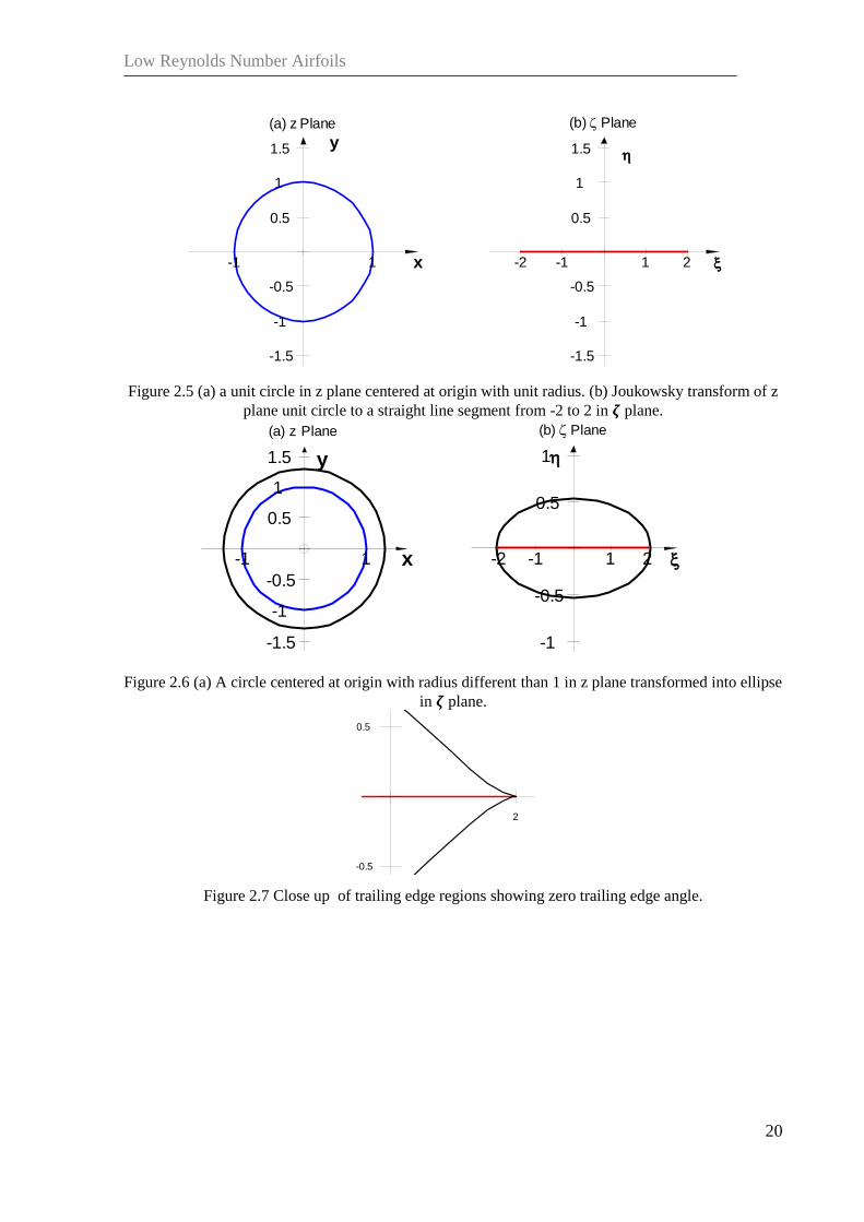
coordinate origin in plane , as shown in Figure 2.5. If this transformation is applied to any
circle in plane which encloses circle with radius then closed curve is obtained in plane
which encloses straight line segment, as shown in Figure 2.6. (note curves from Figure 2.5 ).
If the larger circle is moved off the center in plane such that it touches the unit circle in one
point as in Figure 2.8 a , then the resulting shape is an ellipse which touches mid-real axis in
plane at one point as in Figure 2.8 b. A symmetric airfoil shape appears in plane if the unit
circle is off centered on real x axis in plane as in Figure 2.9. The camber is added to the
airfoil shape if the center of the unit circle is off the origin in both and . in plane, see
Figure 2.10. The airfoil shapes obtained by Joukowsky transform in Eq.( 2.37) are cusped at
the trailing edge, as can be seen in Figure 2.7 which makes them impractical. Karman-Trefftz
transform can be used to form airfoils with non zero trailing edge is reviewed in the next
section.
Low Reynolds Number Airfoils
20
Figure 2.5 (a) a unit circle in z plane centered at origin with unit radius. (b) Joukowsky transform of z
plane unit circle to a straight line segment from -2 to 2 in plane.
Figure 2.6 (a) A circle centered at origin with radius different than 1 in z plane transformed into ellipse
in plane.
Figure 2.7 Close up of trailing edge regions showing zero trailing edge angle.
(a) z Plane
-1 1
-1.5
-1
-0.5
0.5
1
1.5
x
y
(b) Plane
-2 -1 1 2
-1.5
-1
-0.5
0.5
1
1.5
(a) z Plane
-1 1
-1.5
-1
-0.5
0.5
1
1.5
x
y
(b) Plane
-2 -1 1 2
-1
-0.5
0.5
1
2
-1.5
-0.5
0.5
1.5

Low Reynolds Number Airfoils
21
Figure 2.8 (a) a circle centered off the origin and has touches the unit circle at one point . (b)
Transformed into an ellipse which touches mid-real axis in plane at one point.
Figure 2.9 (a) a unit circle with center offset on real x axis in plane (b) A non cambered airfoil in
plane.
Figure 2.10 (a) circle with center off the origin in both and .with part of the contour
outside the unit circle (b) Cambered airfoil in plane with part of its contour above real axis.
2.4 Karma-Trefftz transformation
This transformation can be used to transform a circle in plane into an airfoil shape in plane
or vise versa. It is given by Eq.( 2.38). The coordinates of singular points and
(a) z Plane
-1 1
-1.5
-1
-0.5
0.5
1
1.5
x-1 1
-1.5
-1
-0.5
0.5
1
y
(b) Plane
-2 -1 1 2
-1.5
-1
-0.5
0.5
1
1.5
-2 -1 1 2
-1.5
-1
-0.5
0.5
1
(a) z Plane
-1 1
-1.5
-1
-0.5
0.5
1
1.5
x
y
(b) Plane
-2 2
-1.5
-1
-0.5
0.5
1
1.5
(a) z Plane
-1 1
-1.5
-1
-0.5
0.5
1
1.5
x
y
(b) Plane
-2 -1 1 2
-1.5
-1
-0.5
0.5
1
1.5

Low Reynolds Number Airfoils
22
are chosen to simplify this figure generation, and
is slightly less than 2,
and is airfoil trailing edge angle. Figure 2.11 is generated by this transformation from a
circle in plane with a center at and a radius of .
( 2.38)
Figure 2.11 Karman-Trefftz transform of an off centered unit circle with and
and radius of 1.0512 in plane into an airfoil, with finite trailing edge angle of 2 deg in plane.
2.5 Flow Analysis over an Airfoil Using Conformal Mapping
The Joukowsky and Karman-Trefftz conformal transformations are used to transform a circle
in z plane into a curve resembling an airfoil in the plane as shown in the above sections.
Theodorsen showed that if inverse transformation is applied to an airfoil in plane, the
resulting curve in z plane will therefore be a near circle. He also showed that the flow about
near circle, and hence the airfoil can be calculated from the flow about the true circle through
an iterative procedure. The basic method is presented in references [12]to [17].
The procedure starts with given airfoil coordinates in plane, flow angle of attack
and free stream velocity . Airfoil coordinates are used to calculate near circle coordinates
using Karman-Trefftz transformation, i.e. from Figure 2.12a to, Figure 2.12b. Every point on
airfoil is conformly mapped to corresponding point on the near circle. There are two singular
points and which are specified midway between airfoil leading edge and center of
curvature, and at airfoil trailing edge, respectively. The near circle shape is transformed to the
origin of the coordinate system after finding its centroid, see Figure 2.12c. Fast Fourier
Transform (FFT) is then used to find relations between the flow in the centered near circle (
plane) and in the plane of the true circle ( plane). The final step, is combining the foregoing
(a) z Plane
-2 -1 1 2
-1.5
-1
-0.5
0.5
1
1.5
x
y
(b) Plane
-2 -1 1 2
-0.1
0.1
0.2
0.3

Low Reynolds Number Airfoils
23
relations to obtain the final expression for the velocity distribution in the airfoil plane in terms
of airfoil coordinates.
The calculation of the velocity distribution about an airfoil is done mainly in few steps. Figure
2.12 shows schematically these steps:
Generation of airfoil shape.
Analytical mapping of airfoil to near circle shape by using Karmen-Traffitz
transformation.
Translation of the near circle to the origin of the coordinate system.
Representing near circle couture as function of true circle this is done iteratively
utilizing Fast Fourier Transform.
Obtaining velocity distribution on true circle and calculate modulus of
transformations.
And finally, calculate pressure distributions over the airfoil surface at given flow angle
of attack and velocity.

Low Reynolds Number Airfoils
24
Figure 2.12 Steps involved in transformations of airfoil to true circle
2.5.1 Airfoil shape
The airfoil coordinates are generated using one of the geometric representation methods
discussed in chapter (5). The points start from the trailing edge through the upper surface to
the leading edge, and then back through the lower surface to the trailing edge. Thus the first
point is same as last point, as illustrated in Figure 2.13. These coordinates are changed to
complex variables in plane and their radius and phase angles are computed
.

Low Reynolds Number Airfoils
25
Figure 2.13 Airfoil generated for conformal mapping
2.5.2 Apply Karman-Trefftz Transformation
The basic relation between the near circle plane ( plane) and the airfoil plane ( plane) is
performed through the Karman-Trefftz transformation ( 2.39) by which corners are removed
from airfoil where
and is airfoil trailing edge angle. Points and are locations
of the singular points. The location of is set med way between leading edge and nose center
of curvature, while is set at the trailing edge. The coordinate of the resulting nearly circular
shape Figure 2.14 is given by . The airfoil coordinates are defined by with the relation
( 2.39)
From which can be expressed explicitly as follows
( 2.40) A
B
Equation ( 2.40) is valid when near the trailing edge upper surface is above real axis and lower
surface is below it. For the points of the lower surface which are above real axis Eq.( 2.40) is
used.
The coordinates of are defined by the relation

Low Reynolds Number Airfoils
26
= ( 2.41)
Where is the radius at any point, and is the angle at that point, as shown in the
Figure 2.12.
Knowing that the above relation can be split into real and imaginary
parts.
Where +
Real part + Imaginary part ( 2.42)
The factor relating velocities in the plane to those in the plane is is called
modulus of transformation and is calculated in later step.
2.5.3 Translation of the near circle to the origin
The center of gravity of the near circular shape is calculated by Eq.( 2.43)
( 2.43)
After calculating the center of gravity, the translated near circle coordinates are obtained by
subtracting from each point.
( 2.44)
Figure 2.14 Airfoil transformed to near circle

Low Reynolds Number Airfoils
27
Figure 2.15 Shifted near circle
Figure 2.16 NACA4412 airfoil transformed to near circle then shifted to origin
2.5.4 Mapping of near circle in plane) to true circle ( plane).
The coordinates of are defined by the relation
( 2.45)
The transformation relating the plane to the plane is the general transformation
-1 -0.5 0 0.5 1-1
-0.8
-0.6
-0.4
-0.2
0
0.2
0.4
0.6
0.8
1Near circle shape (Karman-Trafittz) in complex plane
Real
Ima
ge
na
ry S1S0
Near circle centered off origin
NACA4412 airfoil
Near circle at origin

Low Reynolds Number Airfoils
28
( 2.46)
But by definition this transformation should result in near circle
( 2.47)
Consequently
( 2.48)
Knowing that
( 2.49)
Substituting
into ( 2.48) we get
( 2.50)
( 2.51)
Equating real and imaginary parts from both sides we obtain
( 2.52)
( 2.53)
These relations show that and are conjugate functions. The true circle radius
is chosen such that there is minimum deviation between points radii on the near circle ψ and
the radius of the true circle which is found from the relation .
( 2.54)
It can be written as
( 2.55)

Low Reynolds Number Airfoils
29
( 2.56)
Where
and
Equations ( 2.55) and ( 2.56) constitute 2N equations, and 2N +2 unknowns. These unknowns
are and where n=1 to N. Other two unknowns are which is related to the true circle
radius R as . In order to place the trailing edge at the real axis ( Equation
( 2.56) will be
( 2.57)
The unknowns can be obtained by applying Fast Fourier transform (FFT) iteratively [20].
Theodorsen originally solved those equations based on interpolation which requires O( )
multiplications, but Fast Fourier Transform simplifies a lot this step with only O(N log N)
multiplications. this approach is used by many authors and found to be efficient [21] [22]
[23] [24]. The main steps involved in the numerical procedure are listed below:
1. Divide the true circle into equally spaced points which is not changed
during the rest of calculation procedure.
2. Find the corresponding points in the centered near circle plane i.e by
iteration.
3. As first step assume that coefficients and are zero i.e coefficients
and , Eq.( 2.56) will reduce to at every point.
4. Since is a known function of at every point in near circle plane i.e. ,
and is known from previous step, the left side of Eq. ( 2.56) is now known.
The right side of this equation is easily computed by using FFT algorithm by
which the coefficients and are obtained, as an estimate.
5. Having obtained coefficients and a new estimate of angle as function
of is possible through Eq.( 2.56). This is done by applying Inverse Fourier
Transform IFFT. In this step new values of are obtained.
6. The value of is obtained by letting at trailing edge. And thus the
angle at trailing edge in near circle plane is .The value of
is obtained directly from FFT algorithm.
Steps 4 through 6 should be repeated until convergence is reached.

Low Reynolds Number Airfoils
30
2.5.5 Calculation of modulus of transformation
The total modulus of transformation is obtained by multiplying modulus of all
transformations.
( 2.58)
1-Airfoil shape is transformed by using analytic Karman-Trefftz transformation Eqn.( 2.40) A
which is function of . Differentiating this equation with respect to we get
as follows
( 2.59)
2- Shifting the near circle plane to origin has a modulus of 1, thus
( 2.60)
3- The third transformation is transformation of near circle to true circle which modulus
of transformation is given by
. Mapping from near circle to circle is performed by the
relation
( 2.61)
But ( 2.62)
and where ( 2.63)
Substituting Eqs( 2.63) and ( 2.62) into Eqs ( 2.61) and substituting for . The expression
can be written in the form
( 2.64)
since θ are functions of and is constant. Thus
and

Low Reynolds Number Airfoils
31
Substituting back into equation ( 2.64) we get
( 2.65)
Where
, to find this derivative we proceed as follows:
Knowing that
Substituting in Eq.( 2.61) we get
Dropping out and taking the log of both sides we get
Separating real and imaginary part we get
It is worth to note that and
Differentiating w.r.t both equations we get

Low Reynolds Number Airfoils
32
If we proceed
Now we can substitute back into Eq.( 2.65)
( 2.66)
( 2.67)
If we further substitute the equations for we will get the following relation
( 2.68)
Equation ( 2.68) represents the modulus of transformation from the near circle plane to the true
circle plane.
2.5.6 Finding velocities in the true circle plane
Flow around true circle with radius of is obtained by the equation
( 2.69)
Conjugate complex velocity on the true circle are obtained with

Low Reynolds Number Airfoils
33
( 2.70)
Since
( 2.71)
( 2.72)
But at the circle surface and at the trailing edge where , Kutta condition must be
satisfied by letting the total velocity to zero and obtaining the required circulation to satisfy
this condition.
Thus
iiii eR
ieeVeV
20 2
( 2.73)
At trailing edge there is a rotation by an angle of and thus the angle of attack will be
modified by this amount. The equation of circulation finally will be
( 2.74)
Circulation necessary to satisfy Kutta condition thus, depends on angle of attack and
position of trailing edge image in circle plane . Having obtained the value of circulation, the
modulus of transformation is calculated by substitution. The last step is to calculate the
velocities in airfoil plane by
( 2.75)
Once velocity distribution is obtained by the above method, pressure distribution is obtained
via the relation
( 2.76)
Sample calculations for Low Reynolds number airfoil E387 are shown in Figure 2.17, Figure
2.18, and Figure 2.19. The pressure distribution calculated by this approach at angle of attack
of degrees and Reynolds number of 300,000 is compared with XFOIL code. Figure 2.20

Low Reynolds Number Airfoils
34
show that the pressure distribution agrees well with XFOIL results. The flow chart for the
above method is summarized in the flow chart shown on Figure 2.21.
Figure 2.17 Potential flow velocity around circular cylinder dw/dz
Figure 2.18 Derivative of transformation (dζ2/dz ) for E387 airfoil.
0 0.1 0.2 0.3 0.4 0.5 0.6 0.7 0.8 0.9 10
0.5
1
1.5
2
2.5
x/c
dw
/dz
0 0.1 0.2 0.3 0.4 0.5 0.6 0.7 0.8 0.9 10.85
0.9
0.95
1
1.05
1.1
1.15
1.2
1.25
1.3
d 2
/d 3
x/c

Low Reynolds Number Airfoils
35
Figure 2.19 Derivative of transformation dz1/ς for E387 airfoil
Figure 2.20 Inviscid pressure distributions at 2o and Reynolds number of 300,000 for E387 airfoil.
0 0.1 0.2 0.3 0.4 0.5 0.6 0.7 0.8 0.90.5
1
1.5
2
2.5
3
3.5
4
4.5
dz
1/
x/c
0 0.1 0.2 0.3 0.4 0.5 0.6 0.7 0.8 0.9 1-1
-0.8
-0.6
-0.4
-0.2
0
0.2
0.4
0.6
0.8
1
x/c
cp
Invicid Pressure distribution = 2
Current calc
Xfoil

Low Reynolds Number Airfoils
36
Figure 2.21 Flow chart for the method of calculation

Low Reynolds Number Airfoils
37
CHAPTER 3
3 Boundary Layer Modeling
As already stated in chapter 2, the assumption of neglecting viscosity leads to two main flow
equations with different levels of complexity. Neglecting viscosity results in calculation of
pressure distribution and lift for airfoils with acceptable accuracy at low angles of attack,
when flow is mostly staying stick to the wall. When angle of attack increases flow separates
and inviscid assumption become less accurate. The other important point is the calculation of
airfoil total drag which is not possible without considering boundary layer flow. Therefore,
this chapter deals with flow inside boundary layer, The first part introduces main concept of
boundary layer, and fundamental integral boundary layer equations. Important boundary layer
phenomena of laminar, turbulent flow transitions, separations are discussed and the method of
solution is also explained. Finally, verification of obtained results are presented.
The separation bubble which constitutes an important part of the boundary layer effort is left
to next chapter.
3.1 Boundary Layer Concept
The boundary layer concept is related back to Ludwig Prandtl in 1904, who noted based on
experimental work that a thin region exists close to the wall when a fluid passes over it. He
divided the flow to two regions, one very close to the wall called boundary layer where all
viscous effects occur. The second layer is inviscid where viscosity effects are negligible, as
seen in Figure 3.1. The boundary layer is the thin region in which, a fluid velocity changes
from zero at the wall to potential flow value at boundary layer edge . In this
region the viscous force are comparably to inertia forces and thus the viscosity effects can’t be
neglected. Outside this region, , the viscous effects can be assumed unimportant, and
the flow can be analyzed as potential flow. The ratio of inertia forces to the viscous forces is
called Reynolds number, defined as
( 3.1)
Prandtl derived the boundary layer equations, by simplifying the Navier-Stokes equations.
The simplification is based on two main assumptions

Low Reynolds Number Airfoils
38
The boundary layer is thin compared to characteristic stream wise dimension
of the body.
where L is the characteristic length of the body and is the
distance from wall where the velocity equals the inviscid stream velocity.
The highest viscous term must have same order of magnitude when compared
with inertia term.
Figure 3.1 Boundary layer concept
It is also further assumed that the pressure change across the boundary layer is small and can
be neglected. Thus the pressure on the wall (inside boundary layer) is assumed equal to that
outside the boundary layer. Hence, the pressure is calculated using potential flow region laws
as depending on stream wise distance x.
( 3.2)
If steady flow is assumed then the pressure is function of x only and the equation reduces to
( 3.3)
Prandtl’s boundary layer equations for steady, two dimensional flow is given by the Eq.s ( 3.4)
together with boundary conditions stated beneath. The first equation is continuity equation,
and the second is momentum equation. The pressure term can be replaced with velocity from
Eq.( 3.3).
( 3.4)

Low Reynolds Number Airfoils
39
Acceleration Pressure Viscous
Forces. Forces. Forces.
B.C.
Where is the viscosity of the fluid. are components of velocity inside boundary
layer in directions, respectively, and is the pressure at distance , as calculated from
potential flow.
3.2 Boundary layer separation
When a region of adverse pressure gradient exists along the flow, the fluid particles decelerate
and cannot continue moving in forward direction. Thus a region of separated flow appears
near the surface and the boundary layer deflects away from the wall into the main stream.
Generally, fluid particles start to move in direction opposite to the external flow [25].
The separation point is defined by the condition when shear stress vanishes or mathematically
when the slop of the velocity gradient at the wall in the normal direction equals zero. This is
shown in Figure 3.2 . a region of reversed flow downstream of separation point.
( 3.5)
Figure 3.2 Separation of boundary layer, defined when the slope of the velocity gradient at the wall in
the normal direction equals zero.
From Prandtl’s boundary layer equations Eq.( 3.4), the left hand side of the second equation
represents the acceleration of fluid particles in the flow. The pressure term will be negative if
is positive, i.e if pressure increases with increasing x, thus the acceleration will be

Low Reynolds Number Airfoils
40
negative, which means that fluid particles will decelerate, and will have low momentum
leading to separation as illustrated in Figure 3.3a.
For steady flows, the flow may separate only when the pressure increases with increasing x,
i.e. only when
the flow separation is possible. If the pressure term is negative fluid
particles will accelerate, hence no separation danger exists, Figure 3.3 b.
(a) Pressure increases
(b) Pressure decreases
Figure 3.3 Velocity distribution in boundary layer at different pressure situations
Laminar boundary layer separations can occur, resulting in turbulent boundary layer.
Turbulence adds shear stresses to the original viscous shear stress due to viscosity; the
additional shear stresses are called Reynolds stresses. First consequence is that similar
solutions in boundary layer are no longer true. Secondly, turbulence may start inside the
separated laminar boundary layer. In this case, the separated shear layer may reach the airfoil
surface and the turbulent flow may reattach again. The region formed after this process is
called a laminar separation bubble (LSB). Laminar separation bubble is known to decrease lift
and increase drag of airfoils, with higher degree as Reynolds number is decreased. Transition
from laminar to turbulent may also occur without bubble formation. Figure 3.4, illustrates this
possibility where airflows on upper and lower surfaces starting from stagnation point.
Laminar boundary layer prolongs for some distance on both surfaces also. On upper surface
the laminar boundary layer separates and flow moves away from the wall forming a
circulatory region before it reattaches again as turbulent boundary layer. Attached turbulent
flow continues until it separates totally from the airfoil surface. Turbulent separation
eliminates the contribution of that portion of the surface from producing lift and produces
more drag due to wake formation.
The lower surface experiences a different scenario. The laminar boundary layer become
turbulent before it separates. This is called natural boundary layer transition. Turbulent flow
continues until trailing edge without separation.

Low Reynolds Number Airfoils
41
The locations on airfoil surface where boundary layer laminar separation, bubble transition,
bubble reattachment, natural transition, and turbulent separation occur are very important
airfoil flow features. They are sometimes called boundary layer features normally measured in
wind tunnels and predicted by computational procedures. For instance, as turbulent separation
point moves toward the airfoil’s leading edge the lift decreases and the drag increases, airfoils
may be designed based on this fact to maximize lift with smooth stall characteristics by
optimizing turbulent separation point movement with angle of attack, or using other boundary
layer feature. One example is given in reference [26].
Figure 3.4 Boundary layer effects
3.3 Shear stress and friction drag
The shearing stress at the wall is defined as
( 3.6)
The viscous drag is obtained from integrating shear stress over the body surface , as given by
Eq. ( 3.7) and shown in Figure 3.5. Taking we get:

Low Reynolds Number Airfoils
42
( 3.7)
Figure 3.5 Viscous drag computation from shear stress
3.4 Boundary layer momentum and energy integral equations
For steady two dimensional incompressible flows, boundary layer momentum equations can
be integrated with respect to from the wall to some height then, after substituting the wall
shear stress from Eqn.( 3.6) , one obtains:
( 3.8)
From the continuity equation the velocity component
, which upon
substitution becomes
( 3.9)
Integration by parts gives
( 3.10)
Substituting we get

Low Reynolds Number Airfoils
43
( 3.11)
Rearranging
( 3.12)
Introducing the definitions
Displacement thickness
( 3.13)
Momentum thickness
( 3.14)
The substitution of these two definitions results in Von Karman integral equations
given by
( 3.15)
The energy integral equation is deduced by K. Wieghadt [100] for laminar boundary layer
flow. It is obtained by multiplying the equations by u and integrating with respect to y,
similarly to the above procedure;
( 3.16)
The second term is treated by integration by parts as
( 3.17)
The first and third parts can be combined
( 3.18)
After integration

Low Reynolds Number Airfoils
44
( 3.19)
The term on the right side represents energy per unit volume and time, dissipated into heat.
Introducing again the dissipation energy thickness δ3 defined as
Energy thickness
( 3.20)
The energy integral equation can be written in the following form
( 3.21)
Which is the energy integral equation for two dimensional laminar incompressible flow in the
boundary layer. For turbulent flow this equation takes the form
( 3.22)
3.4.1 Boundary layer integral approach
The boundary layer integral parameters are
( 3.23)
The displacement thickness represents the displacement of boundary layer, and the
momentum thickness is related to the friction drag from stagnation point up to the
position . The energy thickness is connected to the energy dissipation in the boundary
layer. The boundary layer separates if velocity near the surface reverses direction. Using these
parameters the integral equations are written as:

Low Reynolds Number Airfoils
45
( 3.24)
Where U is potential flow velocity at location x, and is skin friction coefficient and is
given by
( 3.25)
The energy equation is also written as
( 3.26)
Where is the dissipation coefficient given by
( 3.27)
If the ratios of the local parameters are also defined as
and
( 3.28)
3.4.2 Laminar boundary layer
The solution method for laminar boundary layer is based on the statement that and
are only function of one parameter. Thus , , and can be expressed as function of the
shape parameter . The following relations hold for skin friction coefficient and dissipation
coefficient, respectively.
( 3.29)
( 3.30)
Where and are given functions of the shape parameter . The Reynolds
number based on boundary layer momentum thickness is defined as
( 3.31)

Low Reynolds Number Airfoils
46
Noting that in dimensionless form of chord based Reynolds number
. Where the
reference velocity is the reference length is the chord , and the reference density is .
[27] .
The relation for are given by the following equations as described by Eppler
works in references [9], and [27] through [30],
If
If
( 3.32)
If
If
( 3.33)
( 3.34)
Equations ( 3.24) and ( 3.26) are coupled ordinary differential equations, which is solved by
numerical integration for and from which the shape factors and are also
calculated. Skin friction coefficient and dissipation coefficient can be obtained from the
calculation using the above equations. The velocity U and it's derivative are imposed by
the potential flow.
( 3.35)
( 3.36)
The shape factor specifies laminar separation. If the velocity U is constant the
value of the shape factor is greater than .
The initial values of solution is given by the Eq. ( 3.37) [27], which corresponds to the first
step of after the stagnation point , where the value is the value of the parameter
at stagnation condition.

Low Reynolds Number Airfoils
47
, ( 3.37)
From which the initial value of the shape parameter in case when boundary layer starts from
stagnation point is given by .
3.4.3 Turbulent boundary layer
The same differential equations can be used for turbulent boundary layer. The relations
between the and and, and are given by [27]:
( 3.38)
( 3.39)
( 3.40)
These relations are derived for Reynolds number range from using
empirical and semi-empirical investigations of turbulent boundary layer done by Ludwieg-
Tillmann. As argued in [27] it is also applicable to outside of upper range but for the lower
range it should be investigated.
Turbulent separation, in this approach, is hardly related to a fixed value of the shape factor
. It is certainly known that for there will be no turbulent separation and for
values of there will be for sure turbulent separation. In the calculations the
turbulent separations is assumed to occur at because it is more reliable for thick
boundary layers, where separations is expected to happen.
It is known that turbulent boundary layer separation depends on Reynolds number,
such that separation occurs later if Reynolds number increases. Laminar boundary layers
separates in much shallower adverse pressure gradient as compared to turbulent boundary
layer.
The friction drag caused by laminar boundary layers is much less than that of turbulent
boundary layer. For these reasons transition from laminar to turbulent is important issue.

Low Reynolds Number Airfoils
48
3.5 Boundary layer transition
Laminar boundary layer separates in mild pressure gradients for which turbulent boundary
layers can resist and stay attached. Skin friction drag, on the other hand, is higher for turbulent
boundary layer. It is a compromise between laminar boundary layer where skin friction drag
is smaller but separation risk is higher and turbulent boundary layer where skin friction drag is
higher with higher separation resistance.. Boundary layer starts usually laminar and then
disturbances grow until it become either separated (laminar separation) or it become turbulent
through either transition (forced or natural transition) or transitional separation bubble. The
LSB becomes more important as Reynolds number is lowered.
Boundary layer transition is connected with stability of so called Tollmien-Schlichting
waves. This stability is function of local Reynolds number based on boundary layer
momentum thickness , which is, defined by Eq.( 3.31) repeated here for convenience.
There exists a critical value of below which no wave will be amplified. This critical
local Reynolds number depends in turn on local velocity profile. Local velocity profiles
without inflation points (which occur normally with favorable pressure gradients) have higher
values of and thus have later transition. In contrast, velocity profiles with inflation point
have lower values of which make transition more likely to happen in flow areas where
separation risk is higher. The velocity profile itself is assumed to be function only of the shape
parameter .
There are two general methods for transition analysis. The first method is based on analysis of
amplification of Tollmien-Schlichting waves which assumes transition when one of the waves
amplifies to the value of . Where N is a specified critical number usually around 10 and
depends on turbulence level in wind tunnels or flight test measurements. Drela [31] developed
a method based on amplification envelopes and implemented it in XFOIL code, this criteria
will discussed in next section.
The second method is empirically derived transition criteria based on local boundary layer
parameters. The transition criterion adopted in this work is the one given in Eppler works. It is
used to predict transition when no laminar separation occurs. If laminar separation is detected
Drela method is invoked in the code.
Equation ( 3.41) which depends on local values of shape factor , which represent velocity
profile shape, local Reynolds number based on , and on roughness factor . The

Low Reynolds Number Airfoils
49
roughness factor may vary from 0 for theoretically very smooth surface to 6 which
represents a highly turbulent air.
( 3.41)
This criterion is plotted on Figure 3.6 for different roughness . Higher values of roughness
factor shifts the curve down which means transition will occur earlier.
Transition is assumed to occur if this criterion is satisfied (area above any red dashed curve).
Flow starts from stagnation point at as shown and as flow develops the shape
factor decreases and increases toward either transition curve (red dashed) or
laminar separation line (blue broken) depending boundary layer development calculations. If
the transition criteria is reached first the calculations switches from laminar closure
correlations Eq.( 3.32) through Eq.( 3.34) to turbulent correlations Eq.( 3.38) through Eq.( 3.40).
Furthermore, if the laminar separation line is attained first a laminar separation bubble
calculations are required. The next section discusses main laminar bubble features and
addresses its effects on airfoil characteristics. Details of adopted LSB molding is discussed in
chapter 5.
Figure 3.6 Eppler Transition criteria for different roughness factor values

Low Reynolds Number Airfoils
50
3.6 Laminar separation bubble
As stated previously, transition could occur through laminar separation bubble, called
sometimes laminar transitional bubble because it acts as a mechanism for transition from
laminar to turbulent flow. Laminar separation bubble happens when laminar flow separates
before transition criteria is reached and flow under goes a transition to turbulent in the
separated shear layer , as illustrated in Figure 3.7. Now turbulent flow has higher momentum
to resist adverse pressure gradients therefore it reattaches again to the surface after some
distance along the airfoil chord. The distance from separation point to reattachment is called
bubble length and the distance from separation to transition is called transition length
where flow is still treated as laminar. Between transition location and reattachment point
with length of the flow is turbulent and there is a considerable velocity change in this
region. The velocity profile at laminar separation point and at reattachment point is defined
for the value of shape factor which corresponds to zero shear stress, as
shown in Figure 3.7.
Figure 3.7 Sketch of laminar separation bubble
The main effects of laminar separation bubble are:
(a) Potential flow velocity distribution is modified by the bubble as shown in Figure 3.8
which suggested by Tani [34] . The solid lines represent velocity distribution without bubble,
and the dashed lines represent the modified velocity. From the separation point to transition
point the velocity is nearly constant , which drops from this value to the intersection
with the solid curve at reattachment. In some cases it was experimentally observed by Dini in

Low Reynolds Number Airfoils
51
[35] and [36] that the reattachment occur with undershoot until the velocity distribution
merges with viscous distribution without bubble. For longer bubbles this velocity distribution
is modified along the bubble length and affects the entire airfoil surface. As Reynolds number
is decreased the first part of the bubble increases in length.
(b) Thickness of separation bubble is shown in Figure 3.7 and it is an important factor
which indicates whether the reattachment will occur or not. It depends on the length . It is
also affected by the potential flow pressure gradient in the region of the bubble. This fact was
studied by Gaster [37] who suggested a non-dimensional parameter . This parameter is given
by
( 3.42)
Where is the value the boundary layer momentum thickness at separation point.
which is the velocity drop along the bubble above which no reattachment can occur.
This drop in velocity is equivalent to adverse pressure gradient in the region after separation
point
, this slope depends on the angle of attack being higher for greater angles of attack
, thus bubble thickness increase with increased angle of attack and decreases as angle of
attack decreases. Furthermore, the location of separation point depends on angle of attack
being more toward the leading edge for higher angles of attack. Therefore, in order to
decrease bubble effects on airfoil performance, it is possible to decrease the operating angle of
attack.
Figure 3.8 Effect of separation bubble on velocity distribution

Low Reynolds Number Airfoils
52
3.7 Eppler’s Bubble prediction method
This method is based on predicting the distance from laminar separation to the point when the
shape factor increases to a value of about 1.6. At reattachment is assumed. A
warning is issued if a bubble exists and its effect on drag is not included.
When the turbulent boundary layer starts after either laminar separation or transition criteria is
reached the turbulent closure relations are directly evoked to solve the same differential
equations. When Separation happens at the shape factor then increases to
higher values following the turbulent closure relations. As shown in Figure 3.9, if the
condition given by the equation is satisfied then a bubble warning is issued.
( 3.43)
Where the value of potential flow velocity at the laminar separation point, and is the
difference between the value of potential flow velocity at separation and reattachment points.
Figure 3.9 Eppler's bubble analogy
3.8 Lift, drag and moment
From the potential flow analysis an inviscid pressure distribution can be obtained
and from the boundary layer calculations shear stress distribution is also obtained. These
two distributions constitute the main sources of all forces and moments affecting airfoil at

Low Reynolds Number Airfoils
53
given flow conditions. Their integration over the surface produces the resultant force and
moment which can be resolved into lift and drag. This reference frame is shown in Figure
3.10 where the pressure distribution acts normal to the surface while the shear stress acts in
the tangent direction. The starting point is chosen at the leading edge which normally different
than stagnation point where boundary layer calculation begins.
The Resultant force is resolved into two coordinate axis systems (1) body axis system
as normal and axial . (2) wind (aerodynamic) axis system as lift and drag . the angle
between them is angle of attack . The relation between these two frames is given by
( 3.44)
Figure 3.10 Sign conventions for pressure and shear stress
Figure 3.11 Body and wind axis systems

Low Reynolds Number Airfoils
54
3.8.1 Integration of pressure and shear stress distributions
If an airfoil of unit span [32] as shown in Figure 3.10 is considered. The integration of
pressure and shear stress is performed from leading edge to trailing edge as follows:
For small element of surface length on the upper surface, there are normal and axial
elemental forces and respectively given as
( 3.45)
For the lower surface
( 3.46)
The normal force N and axial force A can be obtained from
( 3.47)
( 3.48)
The moment can obtained in similar manner , keeping in mind sign convention when the
reference point is the leading edge is positive when increasing angle of attack, and using the
non dimensional coefficients the following working form is obtained, and
and reference area and is the airfoil chord.
( 3.49)
( 3.50)
( 3.51)
From which the aerodynamic coefficients and are obtained with the equations:
( 3.52)

Low Reynolds Number Airfoils
55
3.8.2 Lift Drag Moment corrections
When viscous separations are present these coefficients are corrected by using Eppler method
[28], as follows: Total drag coefficient is calculated from boundary layer solution data
evaluated at trailing edge using Squire and Young formula [33] which is modified for high
values of H12 which was found to produce better results. And also corrected when separations
exists [27].
( 3.53)
Where
( 3.54)
Equation ( 3.53) when applied to each surface results in drag due to that surface. The sum of
upper and lower surfaces results in total drag on airfoil.
The greatest effect on aerodynamic comes from boundary layer separation than that from
boundary layer thickness. Thus when high separations exists on upper surface lift coefficient
corrections are applied in which angle of attack is modified. The lift coefficient correction is
computed based on the separated distance travelled by air on the surface which is used to
find out the angle of attack correction.
( 3.55)
Where, is the slope of the upper surface at the area close to trailing edge, and is the
angle of attack relative to chord line, as shown in Figure 3.12. Lift coefficient is modified for
the upper and lower surfaces using the Eq.( 3.56) . The lift correction on upper surface is
always negative and always positive for the lower surface, so lift is reduced in both cases.
( 3.56)
The moment coefficient is also corrected in similar manner using the relation
( 3.57)

Low Reynolds Number Airfoils
56
Figure 3.12 Lift and moment corrections due to boundary layer separation
3.9 Comparison of turbulent closure relations
The calculation of turbulent boundary layer using two Von Karman momentum and energy
equations, with five unknowns, namely additional closure relations are
required. For turbulent boundary layer, Drela has developed a shape factor relations [31]. One
important parameter is the dissipation coefficient , which depends on the distribution of
Reynolds stresses in the boundary layer. The Reynolds stresses in turn depend on the
upstream conditions. In order to take into account these effects Drela used Greens lag
equation to calculate the maximum shear stress coefficient. from which the dissipation
coefficient is computed. An additional differential equation is thus, added to the two Von
Karman integral boundary layer equations. This equation has the form:
( 3.58)
It is worth to note that these models are modified from time to time and there exists different
forms of the equations and coefficients. For example the above equation only the first term is
used by Dini [35] with a coefficient of 4.2 instead of 5.6.
In the rest of this section a comparison is shown between Drela as presented by Dini ,
modified Drela as presented by Lutz and Wagner [38], and finally Lutz & Wagner model. All
these models are derived for incompressible turbulent boundary layer flows. Eppler’s model is
independent of and presented here for reference. It can be seen that at high local
Reynolds number of 5000, Figure 3.13 ,the three models match and produce same results. As
the local Reynolds number based on momentum thickness is decreased to about 400 – 275 the
Drela model separates from other models and still produce same results, as shown of Figure

Low Reynolds Number Airfoils
57
3.14 and Figure 3.15. Further decrease of to about 200 - 100 Drela models produce
different results and even deviate from the known limit, as seen on Figure 3.16 and Figure
3.17 and supported by Lutz and Wagner work , Figure 3.18.
As a conclusion the above presented Drela models should not be used in low range
below about 400. Lutz and Wagner seem to produce acceptable results at this range of local
Reynolds number.
3.9.1 Eppler turbulent model:
The relations between the and and, and are given by Eppler, These relations does
not depend on .
( 3.59)
( 3.60)
( 3.61)
3.9.2 Drela Turbulent closure
Following Dini because of completeness of expressions and report,
( 3.62)
The maximum shear stress is for equilibrium state is obtained using
( 3.63)
The value of is given by the equation
( 3.64)
The closure relation
( 3.65)
Where

Low Reynolds Number Airfoils
58
( 3.66)
( 3.67)
( 3.68)
( 3.69)
( 3.70)
for
for
( 3.71)
Where
( 3.72)
( 3.73)
( 3.74)
( 3.75)
( 3.76)
( 3.77)

Low Reynolds Number Airfoils
59
3.9.3 Modified Drela model used by LUTZ and Wagner [38]
for ( 3.78)
Where
( 3.79)
3.9.4 Lutz and Wagner model
This model is published in [38] , and they claimed that it produces good results compared
with Drela model at low local Reynolds number, such that is always greater than 1.
for ( 3.80)
( 3.81)
( 3.82)
Figure 3.13 Comparisons of different shape factor relations for incompressible turbulent boundary
layer at
1.4 1.5 1.6 1.7 1.8 1.9 21
1.5
2
2.5
3
3.5
4
4.5
5
H32
H12
comparison of turbulent boundary layer clouser relations Re2
= 5000
Eppler
Lutz&Wagner
Drela Dini
Drela L&W

Low Reynolds Number Airfoils
60
Figure 3.14 Comparisons of different shape factor relations for incompressible turbulent boundary
layer at
Figure 3.15 Comparisons of different shape factor relations for incompressible turbulent boundary
layer at
1.4 1.5 1.6 1.7 1.8 1.9 21
1.5
2
2.5
3
3.5
4
4.5
5
H32
H12
comparison of turbulent boundary layer clouser relations Re2
= 400
Eppler
Lutz&Wagner
Drela Dini
Drela L&W
1.4 1.5 1.6 1.7 1.8 1.9 21
1.5
2
2.5
3
3.5
4
4.5
5
H32
H12
comparison of turbulent boundary layer clouser relations Re2
= 275
Eppler
Lutz&Wagner
Drela Dini
Drela L&W

Low Reynolds Number Airfoils
61
Figure 3.16 Comparisons of different shape factor relations for incompressible turbulent boundary
layer at
Figure 3.17 Comparisons of different shape factor relations for incompressible turbulent boundary
layer at
1.4 1.5 1.6 1.7 1.8 1.9 21
1.5
2
2.5
3
3.5
4
4.5
5
H32
H12
comparison of turbulent boundary layer clouser relartions Re2
= 200
Eppler
Lutz&Wagner
Drela Dini
Drela L&W
1.4 1.5 1.6 1.7 1.8 1.9 21
1.5
2
2.5
3
3.5
4
4.5
5
H32
H12
comparison of turbulent boundary layer clouser relations Re2
= 100
Eppler
Lutz&Wagner
Drela Dini
Drela L&W

Low Reynolds Number Airfoils
62
Figure 3.18 Comparisons of different shape factor relations for incompressible turbulent boundary
layer, from reference [38]

Low Reynolds Number Airfoils
63
3.10 Verification of boundary layer calculations
3.10.1 Comparison with Eppler code
Boundary layer calculations are verified by comparison with Eppler code results as for Eppler
airfoil E1098 which shown in Figure 3.19. The velocity distribution shown in this figure is
that obtained from Eppler code for the propose of boundary layer computations, such that any
differences in velocity calculation methods between current calculations and Eppler's
calculations will be avoided.
Figure 3.19 Eppler airfoil E1098 and velocity distribution at Re 1E06 and
Boundary layer development is compared in terms of main parameters which is the shape
factor and the boundary layer momentum thickness as function of surface distance for
both upper and lower surfaces as shown in Figure 3.22 through Figure 3.25. They
comparisons show identical shape and trend of variation of the parameters on both upper and
lower surfaces. Since drag is computer using these parameters the comparison of drag is
0 0.1 0.2 0.3 0.4 0.5 0.6 0.7 0.8 0.9 10
0.5
1
1.5
2Velocity distribution at Reynolds number of 1E06 and zero angle of attack
x/c
V
0 0.1 0.2 0.3 0.4 0.5 0.6 0.7 0.8 0.9 1-0.1
-0.05
0
0.05
0.1
0.15Eppler E1098 airfoil
y/c

Low Reynolds Number Airfoils
64
illustrated for three angle of attack together with transition point location on upper surface on
the following table. The results are identical for this airfoil at these conditions. The transition
point location values seem to be overestimated, the reason may be related to the very fine
integration step used in Eppler code close to separation point. Figure 3.26 through Figure 3.28
show other important boundary layer parameters calculated on lower and upper surface for
reference.
Table 3.1 Comparisons of total drag and transition point location on upper surface at Re=1e06
Figure 3.20 Comparison of drag coefficient for E1098 at between current calculation and
Eppler code.
2 4 80
0.002
0.004
0.006
0.008
0.01
0.012
[deg]
cd
Eppler
Current calc
ALFA
CD total Upper Transition point location
Current Eppler Current Eppler
0 .0106 .0104 0.57736 0.4549
2 .0072 .0071 0.58 0.4597
8 .0081 .0079 0.5722 0.4794

Low Reynolds Number Airfoils
65
Figure 3.21 Comparison of location of upper surface transition point for E1098 at between
current calculation and Eppler code.
STR = for Eppler E1098 airfoil at Re1M and zero angle of attack used in verification
Figure 3.22 comparisons over E1098 airfoil upper surface at Re 1E06 ,
2 4 80
0.1
0.2
0.3
0.4
0.5
0.6
0.7
[deg]
transitio
n location
Eppler
Current calc
0 0.1 0.2 0.3 0.4 0.5 0.6 0.7 0.8 0.9 1
1.5
1.55
1.6
1.65
1.7
1.75
Surface distance
H3
2
H32
develpment on upper surface of E1098 airfoil at =0 Re=1M
Eppler code
current code

Low Reynolds Number Airfoils
66
Figure 3.23 comparisons over E1098 airfoil lower surface at Re 1E06 ,
Figure 3.24 comparisons over E1098 airfoil upper surface at Re 1E06 ,
0 0.1 0.2 0.3 0.4 0.5 0.6 0.7 0.8 0.9 1
1.5
1.55
1.6
1.65
1.7
1.75
1.8
Surface distance
H3
2
H32
development on the lower surface of E1098 airfoil at Re1M and =0
Current code
Eppler code
0 0.1 0.2 0.3 0.4 0.5 0.6 0.7 0.8 0.9 10
1
2
3
4
5x 10
-3
Surface distance
2
2 develpment on upper surface of E1098 airfoil at =0 Re=1M
Eppler Code
Current Code

Low Reynolds Number Airfoils
67
Figure 3.25 comparisons over E1098 airfoil lower surface at Re=1E06 ,
Figure 3.26 shape factor development over E1098 airfoil surfaces as calculated
0 0.1 0.2 0.3 0.4 0.5 0.6 0.7 0.8 0.9 10
1
2
3
4
5
6
7
8
9x 10
-3
Surface distance
2
2 development on the lower surface of E1098 airfoil at Re1M and =0
Current code
Eppler code
0 0.2 0.4 0.6 0.8 11
1.5
2
2.5
3
H12
development on the surface of E1098 airfoil at Re1M and =0
Surface distance
H1
2
Upper surface
Lower surface

Low Reynolds Number Airfoils
68
Figure 3.27 Reynolds number based on over the airfoil surface
Figure 3.28 Reynolds number based on over the airfoil surface
0 0.1 0.2 0.3 0.4 0.5 0.6 0.7 0.8 0.9 10
1000
2000
3000
4000
5000
6000
7000
Red
2
development on the surface of E1098 airfoil at Re1M and =0
Surface distance
Re
d2
Upper surfcae
Lower surface
0 0.1 0.2 0.3 0.4 0.5 0.6 0.7 0.8 0.9 10
1
2
3
4
5
6
7
8x 10
-3 Cf development on the surface of E1098 airfoil at Re1M and =0
Surface distance
Cf
Upper surface
Lower surface

Low Reynolds Number Airfoils
69
3.10.2 Comparisons with XFOIL code
It is known that Eppler code does not take the additional drag due to the separation bubble
into account. Instead it creates a bubble warning . And the user should that the drag values are
under estimated. Since laminar separation phenomenon is not taken care of ,yet, by the code
it is interesting to see the comparison of boundary layer parameters with XFOIL code which
uses different laminar and turbulent closure relations and do account for separation bubble
affects. The boundary layer parameters comparisons are performed for NACA 4412 at
Reynolds number of 1E06 and angle of attack of 2 degrees shown in Figure 3.29. The shape
factor is compared to XFOIL in Figure 3.30. It is interesting to see that the values are in
close agreement up to the laminar separation point, after which values predicted by XFOIL
code grow to approximately 4 (inside the bubble) while values from current computations
predict a sharp decrease in values. The reason being that for XFOIL predictions
increases up to the point of transition which is some distance backward of the laminar
separation point while current computations assume transition just at laminar separation
point. After a chord distance of 0.6 both curves agree and have similar trend and values,
accept at trailing edge. This is expected since after this distance the boundary layer has
reattached and is in equilibrium state thus both turbulent closure relations give similar results.
The above differences in the key solution parameter has manifested in the boundary layer
momentum thickness and the skin friction coefficient as shown in Figure 3.31 and
Figure 3.32 respectively. Next chapter deals with laminar separation bubble modeling.
Figure 3.29 NACA 4412 airfoil shape and velocity distribution using current calculation
0 0.1 0.2 0.3 0.4 0.5 0.6 0.7 0.8 0.9 1-0.05
0
0.05
0.1
0.15NACA 4412 airfoil shape and inviscid velocity profile
y/c
0 0.1 0.2 0.3 0.4 0.5 0.6 0.7 0.8 0.9 10
0.5
1
1.5
x/c
V

Low Reynolds Number Airfoils
70
Figure 3.30 Comparisons of shape factor ,
Figure 3.31 Comparisons of boundary layer thickness
0 0.2 0.4 0.6 0.8 1 1.2 1.41
1.5
2
2.5
3
3.5
4
upper surface distance
H1
2
Shape factro H12
development note the bubble extends approximatlly from 0.42 to 0.6
Xfoil Calculation
Current calc. without Sep. Bubble
0 0.2 0.4 0.6 0.8 1 1.2 1.40
0.005
0.01
0.015
Upper surface distance
2
2 development note the bubble extends approximatlly from 0.42 to 0.6
XFOIL code
Current calc. without Sep. Bubble Model

Low Reynolds Number Airfoils
71
Figure 3.32 Comparisons of skin friction coefficient on upper surface
0 0.2 0.4 0.6 0.8 1 1.2 1.4-2
0
2
4
6
8
10
12
14
16x 10
-3
Upper surface distance
Cf
Cf development note the bubble extends approximatlly from 0.42 to 0.6
XFOIL code
Current calc. without Sep. Bubble Model

Low Reynolds Number Airfoils
72
CHAPTER 4
4 Laminar Separation Bubble modeling
A laminar separation bubble appears on airfoil surfaces when an attached laminar boundary
layer is subjected to an adverse pressure gradient of specific magnitude that causes the flow to
separate before transition occur. The separated laminar flow soon reattaches after being
transformed to turbulent in a region away from the airfoil surface. This phenomenon is more
important as Reynolds number is decreased, as noted by Shyy [55]. It is considered a
challenge to low Reynolds number airfoil aerodynamics predictions. Laminar separation
bubble is first noted by Jones (1933) [39] when he studied airfoil stall process. Since then,
extensive experimental and theoretical investigations of the laminar separation bubble
structures are performed. Leading edge bubble were first studied because it was believed to
cause sudden airfoil stall at low speeds. Owen [41], Crabtree [46], Gaster [49] [50], Horton
[52] [53] are among the first who contributed to laminar separation bubble research.
Mc Cullough and Gault [54] related the stall type with boundary layer features. According to
their analysis, there are three types of stall that depend on boundary layer characteristics.
Trailing edge stall occurs when turbulent boundary layer separation point leaves the trailing
edge and moves forward. Whereas, in leading edge stall laminar boundary layer separates
near leading edge without subsequent reattachment. The third type of stall is called thin airfoil
stall when the separated laminar boundary layer reattaches (as turbulent boundary layer) and
the turbulent reattachment point moves toward the trailing edge as the angle of attack is
increased causing decreased lift which limits aircraft operations at low speeds [53].
Recently, remotely piloted vehicles (UAVs), Micro Air Vehicles (MAVs) and wind turbine
applications mostly operate at Reynolds number range below 1 million, as argued by Muller
[51], Figure 4.1. At this Reynolds number range laminar separation bubble may appear on
airfoil near mid chord, causing a significant decrease in lift and increase in drag. Due to this
reason general aviation airfoils does not perform well for these applications, and low
Reynolds number effects, such as, bubble formation, its structure ,separation, transition and
reattachment conditions has to be studied.
Classically laminar separation bubbles are classified as short and long bubbles, see the review
by Tani [40]. Bubbles are alternatively classified depending on their effect on inviscid
pressure distribution rather than on its length. Laminar separation bubbles may show local

Low Reynolds Number Airfoils
73
pressure distribution change (Weak bubbles) or it may significantly alter the pressure
distribution (strong bubble).
It is the estimation of increased drag and the investigation of type of airfoil stall that motivate
most of recent laminar separation bubbles studies. These methods vary from issuing a
warning so that the designer may suggests airfoil shape modifications to the evaluation of
global bubble effects on pressure distribution.
Horton was the first who presented laminar separation bubble structure as can be seen in
Figure 4.2. The flow at low Reynolds number usually starts laminar and thus is more likely to
separate. Thus a mild pressure gradient will cause laminar boundary layer separation just after
maximum velocity point. The separation never happen in the favorable pressure gradient part,
it always happens in adverse pressure gradient region. The boundary layer moves away from
the wall as a result of separation creating a region of approximately stagnant air followed by
reversed flow region.
Figure 4.1 Chord Reynolds number Vs. flight speed for different natural and manmade objects

Low Reynolds Number Airfoils
74
Figure 4.2 A schematic shape of short laminar separation bubble. [52]
The flow undergoes a transition to turbulent at a point above this region in the shear layer.
The turbulent flow as known with higher mixing and more resistance to separation may
reattach to the surface after some distance along the surface from the transition point. If the
flow reattaches again a laminar separation bubble is formed, but if the turbulent flow fails to
reattach to the surface the turbulent boundary layer continue separated (sometimes this it is
understood as a long bubble which extends into the wake). Laminar separation bubble length
decrease with an increase of angle of attack up to a point when it suddenly increases. This
phenomenon is called bubble bursting and is explained as a failure of turbulent boundary
layer to reattach again to the surface. Laminar separation bubble bursting causes high and
sudden drop in lift and an increase in drag. A typical pressure distribution is shown in Figure
4.3.
Gaster has related this phenomenon to the boundary layer conditions at separation. He
developed an empirical relation between and Gaster parameter P given by Eqn. ( 4.1),
which expresses the average velocity gradient over the length of the bubble. He found from
experimental measurements analysis that at bursting P is a function of at separation.
( 4.1)
Where and are the velocities at separation and reattachment points respectively. L is the
bubble length defined as the surface distance from separation point to reattachment.

Low Reynolds Number Airfoils
75
Figure 4.3 Effect of long and short bubble at high Reynolds number [51]
While, short bubble affects mostly the stall behavior of airfoil long bubble has an un-preferred
effect on the entire polar.
Numerical methods are also used by many authors such as Cebece [42], Alam & Sandham
[43], Jones [44], Cadieux [45] to investigate numerically bubble formation and effects. They
predicted bubble structure in two dimensional flow in order to simulate experiments. In some
cases three dimensional studies are performed as flow is really three dimensional on wing
sections. Alam, used Direct Numerical Simulations (DNS) to study short laminar separation
bubbles [46]. Crivellini has. Studied laminar separation bubble on low Reynolds number
operating airfoils using RANS modeling by means of an high-accuracy solver and
experimental verification [47].
Although, numerical methods provide large quantity of detailed information about the flow, it
is not used as routine methods, as it requires more effort in domain size selections and grid
sensitivity analysis, in addition to the choice of turbulence models. Bubble forcing method
also has an effect on obtained results. Due to these reasons it is hard to be used for
optimization purposes especially if many shapes is to be analyzed. It is more suitable if a
given shape is to be analyzed such that experimental measurements are more focused and
specific. In the last decades successful airfoil designs for different applications were possible
using inviscid-viscous interaction methods followed by experimental measurements.
Airfoil design, analysis and optimization will require the development of laminar separation
bubble model that is faster than finite differences or N-S equation solvers. Dini used an
inviscid–viscous interaction model to predict effects of laminar separation on airfoil drag at

Low Reynolds Number Airfoils
76
low Reynolds numbers. The method is based on the hypothesis that laminar separation
bubble can be modeled using local flow parameters. Boundary layer development a head of
the bubble is performed to predict both separation conditions and forward disturbances
information needed to predict transition. This method shows very good accuracy regarding the
prediction of the modified inviscid distribution and the increase in drag in the range of
Reynolds number as low as 100,000 [35]. This range represents most interesting operational
range of UAV’s and wind turbines, as argued by Muller’s in Figure 4.1.
Drela and Giles used interactive methods that make use of integral boundary layer
formulation these methods provide efficient solution procedures, with accuracy contained
within boundary layer assumptions applicability. Eppler also uses this formulation to issue a
warning of expected bubble effect on airfoils. Eppler’s method is used successfully to design
airfoils for many applications in the past for Reynolds number 500,000 and higher. For lower
Reynolds numbers, however, it is difficult to use this criteria to eliminate bubble by
modifying the shape of airfoil since laminar separation bubble is always present at Reynolds
number lower than 500,000 [51]. Therefore, an improvement in LSB prediction will result in
better estimation of aerodynamic characteristics at this range.
4.1 Reynolds number and angle of attack variation
At higher Reynolds numbers natural flow transition from laminar to turbulent inside the
boundary layer happens very quickly in the favorable pressure region, where no laminar
separation risk is expected. The turbulent boundary layer is more resistant to adverse pressure
gradients and usually flow may separate close to the trailing edge (Turbulent separation), as
seen in Figure 4.4. As the angle of attack is increased this separation point moves forward and
as a result airfoil lift decreases. The resulting lift curve has smooth shape indicating smooth
airfoil stall.
Figure 4.4 High Reynolds number flow over a large wing

Low Reynolds Number Airfoils
77
At lower Reynolds numbers laminar boundary layer continue inside the region of adverse
pressure gradient, without transition. At some point laminar separation may occur and the
boundary layer moves away from the airfoil surface, see Figure 4.5 for which angle of attack
is small and the flow transition occurs far from the wall. Turbulent reattachment occur after
that and turbulent flow continue to the trailing edge. Figure 4.6, shows a case when higher
angle of attack is encountered where bubble is shorter and closer to the leading edge. Figure
4.7 shows a case when the bubble bursts and airfoil stalls. Airfoil characteristics are affected
by stall type and bubble length. Figure 4.3 shows effect of short and long bubble on drag polar
and lift curve. While, short bubble affects mostly the stall behavior of airfoil long bubble has
an un-preferred effect on the entire polar. It is thus avoided in the design process.
Figure 4.5 Low Reynolds number flow at low angle of attack
Laminar separation occur during adverse pressure gradient, followed by transition and
subsequent reattachment resulting in additional drag.
Figure 4.6 Low Reynolds number flow over airfoil at higher angle of attack, a case when higher angle
of attack is encountered where bubble is shorter and closer to the leading edge

Low Reynolds Number Airfoils
78
Figure 4.7 Low Reynolds number flow at stall, when the bubble bursts, airfoil stalls and airfoil
characteristics are affected by stall type and bubble length.
4.2 Laminar separation bubble model
The model adopted in this work is developed by Dini [35]and [36], in which a weakly
interacting laminar separation bubble in two dimensional incompressible flow over airfoils is
modeled. The main aim of the model is to compute the increased airfoil drag that result from
bubble formation.
A weakly interacting bubble is characterized by dominant local effect on pressure distribution.
The model focus on the calculation of the shear layer through different bubble parts as
illustrated in the following sections. Laminar separation bubble starts when a laminar flow
separates, at a point , causing the boundary layer to move away from the airfoil surface, see
Figure 4.8. The point of laminar separation can be predicted by the solution of integral
boundary layer method described in chapter (2). The shear layer grows until transition from
laminar to turbulent occurs at point T. The region between points S and T is characterized by
presence of velocity plateau distribution shown on Figure 4.8. The location of transition is to
be calculated since it determines the bubble length and thus bubble drag. The surface distance
between the point of separation and the point of transition is denoted by . After transition
occurs at point the flow becomes turbulent and the pressure recovers leading to
reattachment at point , with length . In many cases, the pressure recovery region is
observed to continue downstream of reattachment point, and the velocity distribution
undershoots the inviscid velocity distribution curve and merges after some distance with
inviscid curve at point , shown on Figure 4.8.
Therefore, the bubble is divided into three regions:
Laminar region that starts from point of laminar separation and ends at point of transition.
Turbulent pressure recovery region, form the point of transition to reattachment.
Undershoot region where the smooth merge of the velocity distribution with inviscid
distribution happen.

Low Reynolds Number Airfoils
79
The main goal is to estimate the drag contribution of the separation bubble. This goal is
established through the correct calculation of the boundary layer momentum thickness
across the above three bubble regions.
Figure 4.8 schematic of bubble and its effects on pressure distribution [dini]
4.2.1 Laminar part of the bubble [36]
The solution of integral boundary layer equations described in chapter (2) is continued until
laminar separation occurs. Laminar separation is indicated when the shape parameter
decreases to the value 1.51509. Starting at this point, the laminar velocity plateau function is
computed based on local boundary layer parameters and as follows:
The average velocity gradient over the bubble area is first estimated form the velocity
distribution. It is defined as the change in velocity
divided by the difference in chord
between the point of laminar separation to the point of reattachment. Since, the point of

Low Reynolds Number Airfoils
80
reattachment is not known at the beginning of the calculation iterative procedure is used to fix
this value.
Reynolds number based on momentum thickness at separation is computed as
( 4.2)
Gaster parameter P is computed depending on the local boundary layer parameters at the
separation point and as
( 4.3)
Where R is chord based Reynolds number, U is inviscid velocity at separation point location
S, and is free stream velocity.
The pressure recovery calculated using experimentally fitted data as shown in Figure 4.9.
and is given by the following equation
( 4.4)
The velocity plateau function is computed starting from separation point until transition is
triggered at point T, and is given by the following equation
( 4.5)
Where is the slope of velocity profile at separation point, and subscript s indicate condition
at separation. The variable S is the surface distance along the airfoil upper or lower side.

Low Reynolds Number Airfoils
81
Figure 4.9 Pressure recovery in the laminar part of the bubble as function of Gaster's pressure
gradient parameter
The boundary layer closure correlations adopted for the laminar part of the bubble are given
by
( 4.6)
( 4.7)
( 4.8)
The integral boundary layer equations (Chapter 2) are solved in direct mode using these
correlations, derived by the above velocity plateau function.
The separation angle γ is defined in Figure 4.10, as the tangent of the separation stream line
that makes with the surface. It is calculated from the empirical relationship proposed
Wortmann (1974) [56] as:
( 4.9)
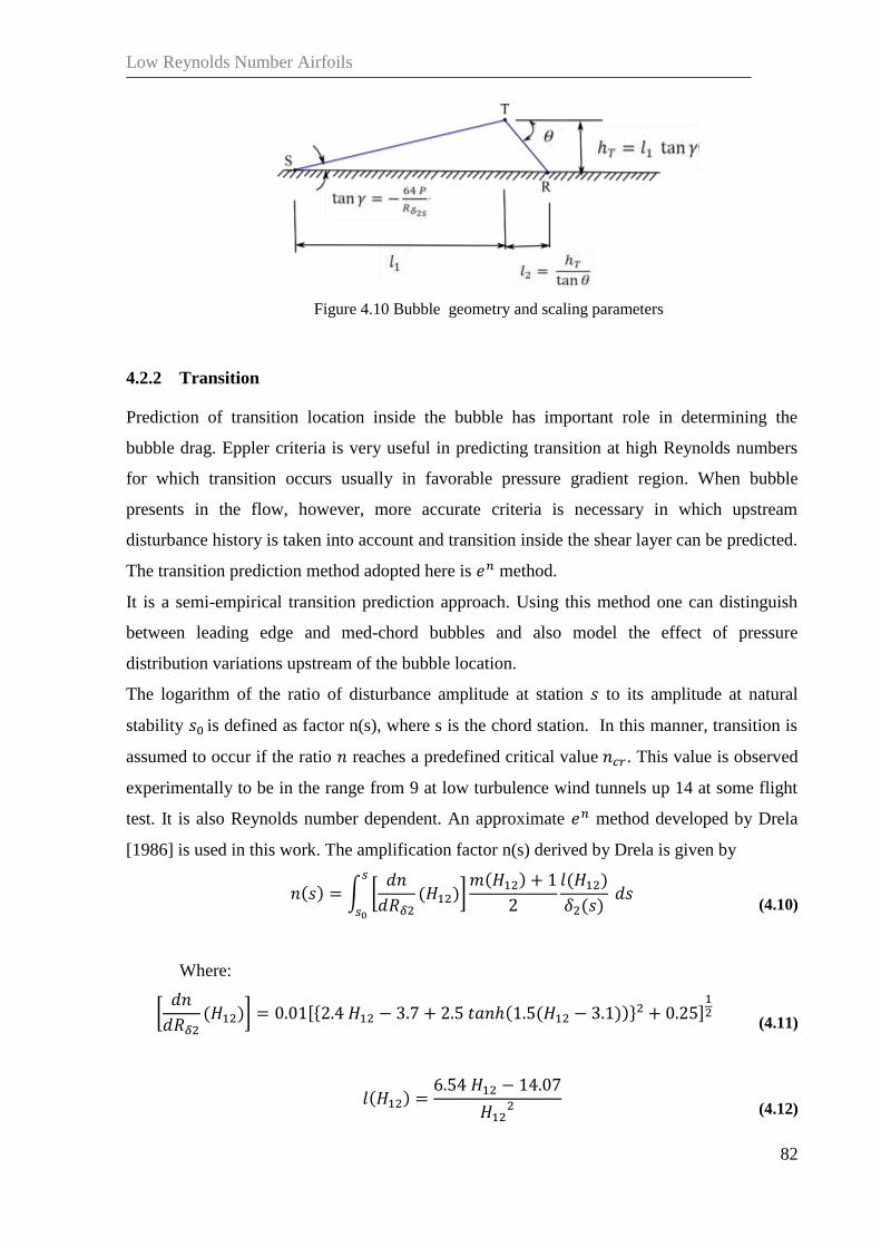
Low Reynolds Number Airfoils
82
Figure 4.10 Bubble geometry and scaling parameters
4.2.2 Transition
Prediction of transition location inside the bubble has important role in determining the
bubble drag. Eppler criteria is very useful in predicting transition at high Reynolds numbers
for which transition occurs usually in favorable pressure gradient region. When bubble
presents in the flow, however, more accurate criteria is necessary in which upstream
disturbance history is taken into account and transition inside the shear layer can be predicted.
The transition prediction method adopted here is method.
It is a semi-empirical transition prediction approach. Using this method one can distinguish
between leading edge and med-chord bubbles and also model the effect of pressure
distribution variations upstream of the bubble location.
The logarithm of the ratio of disturbance amplitude at station to its amplitude at natural
stability is defined as factor n(s), where s is the chord station. In this manner, transition is
assumed to occur if the ratio reaches a predefined critical value . This value is observed
experimentally to be in the range from 9 at low turbulence wind tunnels up 14 at some flight
test. It is also Reynolds number dependent. An approximate method developed by Drela
[1986] is used in this work. The amplification factor n(s) derived by Drela is given by
( 4.10)
Where:
( 4.11)
( 4.12)

Low Reynolds Number Airfoils
83
( 4.13)
and is the location at which which is defined with the following
function
( 4.14)
During the boundary layer development the value of , are available at each point .
Thus, is calculated at each point using Eq.( 4.14). The chord station at which
is taken as the lower integration limit in Eqn.( 4.10). Therefore at this point the
computation of value of the amplification factor starts. Drela added this equation to the
system of equations that are solved by finite difference in XFOIL code [57]. When integral
boundary layer approach is adopted, like in this work, the amplification factor is
computed by integrating this equation with the boundary layer integral equations.
The integration continue until the value of equals the predefined value , at
which transition from laminar to turbulent is assumed. And the code switches to calculation of
turbulent part of the bubble. In wind tunnels it was reported that n=9 is an accurate
approximation.
The transition point corresponds to the highest point of the bubble , and the surface length
from the separation point to this point corresponds to the laminar part of the bubble . The
bubble height at transition is given by the empirical relation
( 4.15)
Where is the separation angle defined by Eq.( 4.9) above.
4.2.3 Turbulent part of the bubble
The turbulent shear layer spreading angle θ is modeled as
( 4.16)

Low Reynolds Number Airfoils
84
When transition location is specified the turbulent length of the bubble is thus
calculated by
( 4.17)
Following this derivation, bubble geometry has the shape shown in Figure 4.10. The
reattachment location is given by the summation of separation and and surface distances.
In order to account for drag increment from the bubble the turbulent part of the bubble is
solved. The solution is based on assumed shape factor in the form given in the Figure
4.11, and formulated by the Eqns.( 4.18) to ( 4.24):
( 4.18)
Where
( 4.19)
( 4.20)
( 4.21)
( 4.22)
( 4.23)
( 4.24)

Low Reynolds Number Airfoils
85
Figure 4.11 normalized shape factor turbulent recovery function
While is calculated based on bubble height at transition, the value of is obtained
iteratively so that the solution merges with inviscid smoothly. The computations is repeated
with different values of A2 until the error in the slope of the obtained velocity distribution and
the inviscid solution is acceptably small, at the point where the two solutions cross each other.
One deg. error was found to be satisfactory.
It is known that the value of the shape factor at separation equals 1.51509 is equivalent to
. The value rises inside the laminar part of the bubble above the value of 4.0 up
to the transition point when it has the maximum value where it starts to decrease to 4.0 again
at reattachment point, as discussed by Drela [58]. The behavior of is just the opposite and
normally presented in the boundary layer development chart after boundary layer calculation
are performed. In fact, in laminar part of the bubble velocity is almost constant, and thus the
pressure, which means that the momentum thickness is almost constant. The variation in
the shape factors in the turbulent part of the bubble reflects a jump in pressure which in turn
produces additional drag, known as bubble drag. If the above mentioned maximum value of
is kept low the resulting increase in drag will be also low. This can be accomplished by
proper choice of velocity distribution in the area around the bubble location. This method is
known as transition ramp normally used in inverse design. This approach can be also utilized
if airfoil design by shape perturbation is selected. A target pressure distribution is pre-
specified and the airfoil shape is found by optimal optimization methods. If a bubble effect is
to be minimized the pressure distribution can be modified in the region ahead and over the
bubble.
The solution of turbulent part of the bubble is performed by integrating the boundary layer
integral equation in inverse mode, derived by the above shape factor model. The integral

Low Reynolds Number Airfoils
86
boundary layer equations in inverse mode are slightly different than standard Von Karman
equations stated in chapter (2). In the turbulent part of the bubble shear stress is the most
important quantity and that is why it is modeled by the shear stress lag equation, which
models the dissipation coefficient in the turbulent boundary layer. The accurate modeling of
dissipation coefficient is necessary to get correct prediction of pressure jump in the turbulent
part of the bubble.
Once the shape factor is calculated, it is used to drive the solution of the system of
equations Eqn.( 4.25) to Eqn.( 4.29) for the variables U, and . Specifically, the abrupt
increase in the value of is of great concern because it will lead to the additional drag, and
thus accounts for transitional bubble effect. It will be shown also in the pressure distribution
which can be compared with measurement.
( 4.25)
( 4.26)
( 4.27)
Where
( 4.28)
( 4.29)
, , and is given by
( 4.30)
( 4.31)
( 4.32)

Low Reynolds Number Airfoils
87
( 4.33)
( 4.34)
( 4.35)
( 4.36)
Where
( 4.37)
( 4.38)
( 4.39)
( 4.40)
( 4.41)
The coefficient is calculated at each point by fitting a parabola between the values at
transition , minimum and at reattachment . Where
( 4.42)

Low Reynolds Number Airfoils
88
4.2.4 Intersection with inviscid distribution
The above procedure is valid for surface points up stream of the reattachment point. The
calculation procedure continues from point of reattachment to the point where the obtained
velocity U curve crosses the inviscid distribution. At crossing, the slopes are compared. If the
difference in slope is greater than 1 deg another value of the factor is used to repeat the
calculations. When the slop difference condition is satisfied the bubble model is terminated.
The integration of the integral boundary layer equations continue using Drela turbulent
closure up to the trailing edge.
If at reattachment the calculated velocity U is higher than the inviscid velocity the merge
happens from above and is not iterated as argued by Dini [35].
4.2.5 Attached turbulent boundary layer
After the intersection with the inviscid profile is established, the integration of the integral
boundary layer equations ( 4.43), ( 4.44), and ( 4.45) is continued in direct mode using the
relations Eq.( 4.46) to ( 4.56)
( 4.43)
( 4.44)
( 4.45)
( 4.46)
( 4.47)
The skin friction coefficient is obtained from the equation
( 4.48)
( 4.49)
( 4.50)

Low Reynolds Number Airfoils
89
( 4.51)
Where
( 4.52)
( 4.53)
( 4.54)
( 4.55)
( 4.56)
The turbulent separation is triggered if the following condition is meet
( 4.57)
The drag is then calculated by squire young formula as
( 4.58)
The computation procedure is best explained through a Figure 4.12 and flow chart Figure
4.13.
Figure 4.12 schematics of possible flow on airfoil with and without bubble

Low Reynolds Number Airfoils
90
Figure 4.13 Flow chart for laminar separation bubble model

Low Reynolds Number Airfoils
91
4.3 Validation of Aerodynamic calculations
Validation is performed by comparison with available experimental data from literature for
incompressible flow at Reynolds number from 200,000 to 500,000 from NASA [59], and
results from Illinois university [60], and [61]. Results are also verified by comparison with
XFOIL code. The inviscid solution obtained from conformal mapping is utilized by
momentum and energy integral equations solver. The resulting drag polar shows good
agreement with experimental data. The computation cost is very small compared to other
methods. The exception is when the interaction between viscous and inviscid is not weak,
particularly close to maximum lift. The location of turbulent separation point is used to
correct the lift and moment coefficients, which is successfully used to design large number of
airfoils in the past. In fact, maximum lift coefficient is over estimated in most of the tested
cases.
The validation process is performed for lift coefficient, drag coefficient, pressure distribution
and boundary layer features for two airfoils at different angles of attack and Reynolds
numbers.
The Eppler E387 airfoil is selected for the comparison since it is widely used in the Reynolds
number range 200,000 to 500,000 and experimental data are available from different wind
tunnels.
Figure 4.14 and Figure 4.15 show comparisons of calculated lift and drag coefficients
compared to experimental measurement from [61] at Reynolds number of 300,000. The
comparison show excellent agreement with experimental measurement both in lift and drag
curves. At this Reynolds number a laminar separation bubble is formed on the airfoil upper
surface during angles of attack up to approximately 7 degrees, as shown in Figure 4.16. The
bubble starts at about med chord and extends to 65% of the chord length. As the angle of
attack is increased the bubble decreases in length and moves toward the airfoil leading edge.
Figure 4.16 also shows a comparison of location of upper surface boundary layer features at
Reynolds number 300,000 at different angles of attack. The figure shows location of laminar
separation points, reattachment points and turbulent separation points. At low angles of attack
current calculations, experimental measurement, and XFOIL results show similar trend for
location of laminar separation and reattachment points. As the angle of attack increases above
8 degrees theoretical calculations fail to predict the short leading edge bubble shown by

Low Reynolds Number Airfoils
92
experimental measurement. The turbulent separation location is very close to the trailing edge
at low angles of attack, as the angle of attack is increased it moves forward in the direction of
the leading edge causing smooth curvature in lift curve and increased drag. Experimental
measurement show a sudden jump in location of turbulent separation location after certain
angle of attack, while current calculations and XFOIL results show smooth variations up to
high angle of attack.
Figure 4.14 versus for for E387 airfoil at Re 300000, Exp from [Summary of Low-Speed Airfoil
Data-2012].
Figure 4.15 versus for for E387 airfoil at Re 300000, Exp from [Summary of Low-Speed Airfoil
Data-2012].
-10 -5 0 5 10 15-0.5
0
0.5
1
1.5
Angle of attack [deg]
cl
Lift variation with angle of attack for E387 ; Re= 300000
calc
Exp
0 0.01 0.02 0.03 0.04-0.2
0
0.2
0.4
0.6
0.8
1
1.2
1.4
cd
cl
Drag polar for E387 ; Re= 300000
calc
Exp

Low Reynolds Number Airfoils
93
Figure 4.16 Comparisons of upper surface boundary layer features for E387 airfoil at Re 300,000
4.3.1.1 Pressure distribution
The pressure distribution calculated by the above method is compared to experimental
measurement at angle of attack of 2 degrees and Reynolds number of 300,000, as shown in
[59]. The laminar separation bubble calculations follow closely the experimental
measurements. The bubble pressure variations is well predicted, the upper surface bubble is
clearly shown, and the lower surface has nearly constant pressure over most of its length.
Reference back to Figure 4.16 the pressure distribution show a large bubble that start at
approximately 0.5c up to .65c. Details of upper surface boundary layer parameters are shown
in Figure 4.19.
0 0.1 0.2 0.3 0.4 0.5 0.6 0.7 0.8 0.9 1-2
0
2
4
6
8
10
12
14
16
x/c
[d
eg
.]
Location of upper surface flow features for E387 airfoil
at Re 300000 [Exp:AIAA 2003-4067]
Turb. Sep XFOIL
Turb. Sep. CALC
Turb. sep. Exp
Lam. Sep. CALC
Reat. CALC
Lam. Sep. Exp
Reat. Exp
Lam. sep. Xfoil
Reat. Xfoil

Low Reynolds Number Airfoils
94
Figure 4.17 comparison of experimental and calculated pressure distribution
for E387 airfoil at Re 300000 and angle of attack 2 deg.
0 0.2 0.4 0.6 0.8 1
-1
-0.5
0
0.5
1
Pressure distribution for E387 airfoil at Re 300000 , =2 deg.
cp
Exp
calc
0 0.2 0.4 0.6 0.8 1-0.05
0
0.05
0.1
x/c
y/c
0 0.2 0.4 0.6 0.8 1
-1
-0.8
-0.6
-0.4
-0.2
0
0.2
0.4
0.6
0.8
1
x/c
cp
E387 airfoil pressure distribution Re 300,000 at alfa= 2
Current calc
Xfoil
Figure 4.18 Comparison of pressure distribution with Xfoil code for E387 airfoil at
Re 300000 and angle of attack 2 deg.

Low Reynolds Number Airfoils
95
4.3.1.2 Boundary layer parameters
Figure 4.19 show upper surface boundary layer parameters as computed by the current code
compared with that calculated by XFOIL. It shows laminar separation point at corresponding
to H32 = 1.51 or H12 =4.The boundary layer momentum thickness variations show sudden
increase inside turbulent part of the bubble as expected. The values of dissipation coefficient
and the friction coefficient are also shown.
Figure 4.20 show upper surface boundary layer development as obtained for the above case.
the points of laminar separation , transition and reattachment are indicated on the chart.
Comparisons with XFOIL code is also presented in Figure 4.21 and Figure 4.22 . shape
factor is XFOIL main shape factor. Comparisons show similar trend and similar maximum
value. The momentum thickness , which is the most important boundary layer parameter
we looked for by this modeling to calculate drag , show good agreement with XFOIL.
Comparisons of friction coefficient , dissipation coefficient , velocity distribution
and
Reynolds number based on momentum thickness show generally good agreement with
XFOIL calculation. Lower surface boundary layer parameters are shown in Figure 4.23 to
Figure 4.26, in which a laminar flow is preserved up to close vicinity to the trailing edge.
Comparisons with XFOIL very close agreement. Boundary layer development chart shown on
Figure 4.26 indicate a laminar separation very close to the trailing edge.
0 0.2 0.4 0.6 0.8 10
0.01
0.02
0.03
cf
x/c
Upper surface cf for E387 airfoil =2 Re =300000
Current
Xfoil
0 0.2 0.4 0.6 0.8 10
0.01
0.02
CD
Upper surface CD
for E387 airfoil =2 Re =300000
Current
Xfoil

Low Reynolds Number Airfoils
96
Figure 4.19 Upper surface boundary layer parameters at Re 300000 and =2 deg. (continued)
0.1 0.2 0.3 0.4 0.5 0.6 0.7 0.8 0.9 1
0
2
4
x 10-3
Upper surafce boundary layer parameters for E387 airfoil =2 Re =300000
2
0 0.1 0.2 0.3 0.4 0.5 0.6 0.7 0.8 0.9 1
1.5
1.6
1.7
1.8
H32
0 0.1 0.2 0.3 0.4 0.5 0.6 0.7 0.8 0.9 10
500
1000
1500
Re2
x/c
0.1 0.2 0.3 0.4 0.5 0.6 0.7 0.8 0.9 1
0
2
4
6
8
H12
0 0.1 0.2 0.3 0.4 0.5 0.6 0.7 0.8 0.9 10
0.5
1
1.5
U/V
Current
XFOIL

Low Reynolds Number Airfoils
97
Figure 4.20 Upper surface boundary layer development chart for E387 at Re 300000 and 2
deg.
Figure 4.21 Comparison of upper surface boundary layer shape factor for E387 at Re
300000 and 2 deg.
0 0.2 0.4 0.6 0.8 10
2
4
6
8
Upper surface H12
for E387 airfoil at =2 Re =300000
x/c
H1
2
Xfoil
Current

Low Reynolds Number Airfoils
98
Figure 4.22 Comparison of upper surface boundary layer momentum thickness for E387 at Re
300000 and 2 deg.
Figure 4.23 Lower surface velocity distribution for E387 at Re 300000 and =2 deg.
0 0.2 0.4 0.6 0.8 10
1
2
3
4
5x 10
-3 Upper surafce 2 for E387 airfoil =2 Re =300000
2
x/c
Current calculations
Xfoil code
0 0.2 0.4 0.6 0.8 10
0.2
0.4
0.6
0.8
1
U /
V
x/c
Lower surface Velocity for E387 airfoil =2 Re =300000
Current
Xfoil

Low Reynolds Number Airfoils
99
Figure 4.24 Variation of momentum thickness for the lower surface of E387 at Re 300000 and 2
deg.
0 0.2 0.4 0.6 0.8 10
0.2
0.4
0.6
0.8
1
1.2
1.4x 10
-3
2
Lower surface 2 for E387 airfoil =2 Re =300000
Current
Xfoil
0 0.2 0.4 0.6 0.8 10
0.01
0.02
0.03
0.04
cf
x/c
Lower surface cf for E387 airfoil =2 Re =300000
Current
Xfoil
0 0.2 0.4 0.6 0.8 10
0.02
0.04
0.06
CD
Lower surafce boundary layer parameters for E387 airfoil =2 Re =300000
Current
Xfoil

Low Reynolds Number Airfoils
100
Figure 4.25 Lower surface boundary layer development parameters at Re 300000 and =2 deg.
0 0.2 0.4 0.6 0.8 10
0.5
1
1.5x 10
-3Lower surafce boundary layer parameters for E387 airfoil =2 Re =300000
2
Current
XFOIL
0 0.2 0.4 0.6 0.8 1
1.5
1.6
1.7
1.8
H32
0 0.2 0.4 0.6 0.8 10
200
400
Re2
x/c
0 0.2 0.4 0.6 0.8 1
2.5
3
3.5
4
H12
0 0.2 0.4 0.6 0.8 10
0.5
1
U/V

Low Reynolds Number Airfoils
101
Figure 4.26 Lower surface boundary layer development chart for E387 at Re 300000 and 2 deg.

Low Reynolds Number Airfoils
102
4.3.2 Variation of aerodynamic coefficients with Reynolds number
Aerodynamic lift and drag coefficients of two airfoils at Reynolds numbers of 200,000
300,000 and 500,000 are plotted in the following figures from Figure 4.27 to Figure 4.32.
Comparisons show generally a good agreement with experimental data. When large
separations are present, however, the current calculations over estimate both lift and drag.
Maximum lift coefficient is over estimated but the angle of attack of maximum lift is
computed with fair accuracy.
Figure 4.27 Comparisons between calculated and experimental drag polar for E387 at Re=200,000.
Figure 4.28 Comparisons between calculated and experimental drag polar for E387 at Re=350,000.
0 0.05 0.1
-0.5
0
0.5
1
1.5 Airfoil E387 ; Re= 199747
cd
cl
-10 0 10 20
-0.5
0
0.5
1
1.5
Angle of attack [deg]
cl
Calc.
Exp.
0 0.02 0.04
-0.5
0
0.5
1
1.5 Airfoil E387 ; Re= 350000
cd
cl
-10 0 10 20
-0.5
0
0.5
1
1.5
Angle of attack [deg]
cl
Calc.
Exp.

Low Reynolds Number Airfoils
103
Figure 4.29 Comparisons between calculated and experimental drag polar for E387 at Re=500,000.
Figure 4.30 Comparisons between calculated and experimental drag polar for S8036 at Re=200,000
0 0.01 0.02 0.03
-0.5
0
0.5
1
1.5 Airfoil E387 ; Re= 500000
cd
cl
-10 0 10 20
-0.5
0
0.5
1
1.5
Angle of attack [deg]cl
Calc.
Exp.
0 0.02 0.04 0.06
-0.5
0
0.5
1
1.5 Airfoil S8036 Re=200000
cd
cl
-10 0 10 20
-0.5
0
0.5
1
1.5
Angle of attack [deg]
cl
Calc.
Exp.

Low Reynolds Number Airfoils
104
Figure 4.31 Comparisons between calculated and experimental drag polar for S8036 at
Re=350,000
Figure 4.32 Comparisons between calculated and experimental drag polar for S8036 at Re=500,000.
0 0.02 0.04 0.06
-0.5
0
0.5
1
1.5 Airfoil S8036 Re=350000
cd
cl
-10 0 10 20
-0.5
0
0.5
1
1.5
Angle of attack [deg]cl
Calc.
Exp.
0 0.02 0.04 0.06
-0.5
0
0.5
1
1.5 Airfoil S8036 Re=500000
cd
cl
-10 0 10 20
-0.5
0
0.5
1
1.5
Angle of attack [deg]
cl
Calc.
Exp.

Low Reynolds Number Airfoils
105
4.3.3 Variation of boundary layer features with Reynolds number
Boundary layer flow features are the positions on the airfoil surface where important changes
happen in the boundary layer flow on upper or lower surfaces, such as location of laminar
separation point, transition point, reattachment point and turbulent separation point. When
laminar separation bubble occurs transition is assumed inside the bubble.
Current calculation results are compared with published experimental data for two selected
airfoils. The first airfoil is Eppler low Reynolds number airfoil E387 which is used as
benchmark for validating low Reynolds number aerodynamic computations. It is extensively
tested in NASA Langley Low Turbulence Pressure Tunnel (LTPT, where drag polar, and
pressure measurements at low Reynolds numbers are published [59]. Recently, E387 airfoil is
tested in the University of Illinois at Urbana-Champaign (UIUC) subsonic wind tunnel [60],
[61], which is intended to validate and refine airfoil low Reynolds number computation
methods. The second airfoil is Selig S8036 low Reynolds number airfoil designed for soft
stall characteristics. Experimental measurement data for these two airfoils at flow Reynolds
numbers are 200,000, 350,000 and 500,000 are used in the validation of current computations.
These measurements include drag polar and location of upper surface boundary layer flow
features.
Comparisons of measured [59] and calculated pressure distributions over E387 airfoil at
Reynolds number of 300,000 and at angles of attack of 4, and 6 degrees are shown in Figure
4.33 and Figure 4.34. The location of the separation bubble is clearly observed on the upper
surface. Calculated pressure distribution agrees with experimental data and XFOIL results.
The bubble location is calculated with acceptable accuracy for optimization computations.
The general observation is that the bubble moves upstream as angle of attack increase, with
length being shorter. Figure 4.18 shows comparisons of locations of upper surface features of
the two airfoils at different angles of attack and Reynolds numbers of 200,000, 350,000, and
500,000.The computed laminar separation, Reattachment, and turbulent separation locations
on upper surface are compared to experimental measurements. Laminar separation and
reattachment locations from XFOIL are also shown for E387 at Reynolds number 350,000.
A laminar separation bubble extends on the upper surface starting approximately at mid
chord. As angle of attack increases the bubble moves toward the leading edge, and its length
decreases. When the bubble length close to leading edge is very short, it could be interpreted

Low Reynolds Number Airfoils
106
as a transition without bubble. Current calculations follow the general trend of both
experimental measurement and XFOIL predictions. As Reynolds number increases the
laminar separation bubble tend to shorten in length, which is in agreement with the general
fact that laminar separation bubble is more dominant in low Reynolds number range. The
results of XFOIL and current calculations seem to under estimate the reattachment point
location, this is also noted [62]. For low angles of attack turbulent separation take place at or
very close to the trailing edge. When angle of attack increases further turbulent separation
moves forward causing high increase in drag and loss in lift.
In all cases turbulent separation point assessed by current computations and XFOIL code at
high angles of attack is more aft than the measured locations. This miss-predictions has the
consequence of over estimating the angle of maximum lift, and thus the value of maximum
lift coefficient.
Figure 4.33 Pressure distribution for E387 at Re 300 000 and 4°
0 0.1 0.2 0.3 0.4 0.5 0.6 0.7 0.8 0.9 1
-1.5
-1
-0.5
0
0.5
1
x/c
cp
Exp
CALC
Xfoil

Low Reynolds Number Airfoils
107
Figure 4.34 Pressure distribution for E387 at Re 300 000 and
0 0.1 0.2 0.3 0.4 0.5 0.6 0.7 0.8 0.9 1
-3
-2.5
-2
-1.5
-1
-0.5
0
0.5
1
x/c
cp
Xfoil
Exp.
CALC

Low Reynolds Number Airfoils
108
Figure 4.35 Comparisons of locations of upper surface flow features for E387 and S8036 at Re
200,000, 350,000, and 500,000. (Solid lines represent experimental data, dashed lines is XFOIL, and
filled symbols are current calculations).
0 0.5 10
2
4
6
8
10
12
14
16
18E387 ; Re 200,000
[
deg.
]
0 0.5 10
2
4
6
8
10
12
14
16
18E387 ; Re 350,000
0 0.5 10
2
4
6
8
10
12
14
16
18E387 ; Re 500,000
[
deg.
]
0 0.5 10
2
4
6
8
10
12
14
16
18S8036 ; Re 200,000
0 0.5 10
2
4
6
8
10
12
14
16
18S8036 ; Re 350,000
x/c
[
deg.
]
0 0.5 10
2
4
6
8
10
12
14
16
18S8036 ; Re 500,000
x/c
CALC
XFOIL
Exp.
CALC
XFOIL
Exp.
CALC
XFOIL
Exp.
Laminer Sep.Turbulent Sep. Reattachment

Low Reynolds Number Airfoils
109
CHAPTER 5
5 Airfoil Parametric Representation
5.1 General Requirement
Parameterization is defined as representing aerodynamic characteristics, such as shape or
pressure distribution, in terms of few numerical parameters. These parameters are called
design variables. Parameterization is often applied to aerodynamic geometric characteristics
of airfoils, wings or even complete configuration. When the design variables are modified the
aerodynamic performance is correspondingly changed. The optimization algorithm and the
designer should look for the design variables that will improve aerodynamic, structure or
flight performance. This process is called optimization. The aerodynamic analysis will lead to
a selection of a set of design variables that satisfies predefined requirements. Each design
variable can change within specified range. Design space is defined by the ranges of all
design variables. For instance, airfoils can be described using NACA representation
(discussed in the next section). Four digit NACA definition uses only 3 parameters to
represent airfoils. The low number of parameters allows fast design and analysis but it may
not cover all possible airfoil shapes. Other airfoil parameterization methods are in use that can
cover more design space and produce improved performance. Conversely, a higher number of
design parameters may lead to improvement in performance, but requires higher
computational cost during the optimization process. Therefore, in many cases tradeoff studies
between computational cost and number of required parameters is necessary. Computational
cost is often measured by number of calls to analysis code. In this work the parameterization
method that will capture a global design space with reduced number of design parameters is
used.
Airfoil parametric representation is considered recently by many authors for use in numerical
optimization and design. One main reason is that aerodynamic analysis codes ask for many
airfoil coordinate points (about 100 points or more). Using these coordinates as design
variables results in non-smooth airfoils which is not aerodynamically acceptable and will also
result in very long optimization time due to large number of design variables. By selecting

Low Reynolds Number Airfoils
110
proper airfoil parametric representation method this problem can be solved. Klfan, [63] stated
a number of factors that are considered during the choice of parametric representation
methods for aerodynamic design. Selection of optimization algorithm, computational cost
required to reach optimum design, and if the optimum design is contained in the design space,
and whether it can be found by search algorithms.
Parametric airfoil representation methods work with parameterization of airfoil shape, which
means that it represent airfoils with few parameters that control airfoil counters. NACA 4
digit airfoil representations uses 3 parameters, PARSEC method uses 11 parameters to
represent upper and lower airfoil surfaces, CST method on the other hand uses a number of
coefficients in polynomial series which can produce rounded leading edge and sharp trailing
edge shapes. The following section describes some airfoil parametric representation methods.
5.2 NACA Airfoil Series
Airfoils shape is defined in a variety of methods. NACA has its own methods of representing
groups of airfoils, such as 4 digit 5 digit or 6 digit series. Reference [65] provides details of
NACA definitions. Although, these airfoils are successfully used in many applications, a need
for airfoil shapes that perform better in for specific applications, such as blade design,
propellers, or at low Reynolds number has derived the research toward other airfoil
representation methods.
NACA airfoils grouped in series such as 4-digit, 5-digit and 6-digit series. Their coordinates
were derived from either geometrical methods using analytical equations that describe the
camber distribution and the thickness distribution along the chord line, see Figure 5.1, or are
derived using theoretical methods like 6-digit series.
5.3 4-digit series airfoils
It is the first series of airfoils designed using this approach. They have 4 digits; the first digit
is denoted by (m) specifies the maximum camber in percent of airfoil chord. The second digit
represents the position of maximum camber (p) in tenths of airfoil chord. The last two digits
represent the maximum airfoil thickness (t) in percent of chord. Thus NACA2412 airfoil, for
example, has 2% camber located at 40% of its chord from leading edge and 12% chord thick.
This representation requires specification of theses 3 parameters to find out the airfoil
coordinates for upper and lower airfoil surfaces. as in Figure 5.1.

Low Reynolds Number Airfoils
111
Figure 5.1 NACA Airfoil Geometrical parameters
The procedure to find the airfoil coordinates is summarized by the following steps and sample
calculations are shown in Figure 5.2 :
a. Chord length is made non dimensional be dividing by chord, thus x varies from 0 at LE to 1
at TE.
b. Using the values of p and m, it is possible to compute mean chamber for each value of x
using the following equations:
for x from 0 to p ( 5.1)
for x from p to 1
( 5.2)
where
yc is camber coordinates.
p - is first digit in NACA designation divided by 100.
m - is the second digit value in NACA designation divided by 10.
t- is the last two digits divided by 100.
c. Compute the thickness distribution around the mean chamber by substituting t into the
following equation:
( 5.3)
d. Calculate the upper ( xu , yu )and lower ( xL , yL )airfoil coordinates using:
0 0.2 0.4 0.6 0.8 1-0.1
-0.05
0
0.05
0.1
0.15
0.2
x/c
y/c
NACA 4 digit airfoils
Lower surface
x=1
(XL ,Y
L)
(XU
,YU
)Upper surface
Mean line
Chord line

Low Reynolds Number Airfoils
112
Figure 5.2 NACA 4- digit airfoil representation parameters
0 0.2 0.4 0.6 0.8 1-0.1
-0.05
0
0.05
0.1
0.15
0.2
x/c
y/c
NACA 4 digit airfoils
m= 5 p= 6 t= 15
m= 0 p= 0 t= 12
m= 2 p= 4 t= 12
Upper surface
Lower surface

Low Reynolds Number Airfoils
113
5.4 PARSEC Method
It is a commonly used method. This method is originally developed by Sobieczky, 1998 [66]
for used in subsonic and transonic airfoils. Its main idea is expressing the airfoil surface as an
unknown linear combination of appropriate mathematical function, and selecting a number of
important geometric characteristics of the airfoil as the design variables, in such a way that
the airfoil shape can be determined from these variables by solving a linear system of
equations. Eleven airfoil geometric characteristics are used to represent airfoil as illustrated in
Table (1) and Figure 5.3.
Table 5.1 Parsec method parameters
rLE Leading edge radius
Xup X location of Upper crest
Yup Y location of Upper crest
Yxxup Upper surface curvature
XLo X location of Lower crest
YLo Y location of Lower crest
YxxLo Lower surface curvature
DYTE Trailing edge thickness
YTE Trailing edge y location
αTE Trailing edge direction
βTE Trailing edge included angle
Figure 5.3 PARSEC method for airfoil parameters
The parsec equation is given by Eq.(1)
( 5.4)

Low Reynolds Number Airfoils
114
Where j takes a value of 1 for upper surface and 2 for the lower surface, the coefficients and
are determined by using the above mentioned airfoil geometric characteristics.
The above equation can be written for the upper and lower airfoil surfaces as follows
( 5.5)
( 5.6)
A specific relations can be derived for the upper and lower surfaces as follows
( 5.7)
1- Leading edge radius
For upper surface
( 5.8)
For lower surface
( 5.9)
2- Trailing edge position
For lower surface
( 5.10)
For lower surface
( 5.11)
3- Airfoil coordinates
( 5.12)
( 5.13)
4-Trailing edge slope
( 5.14)

Low Reynolds Number Airfoils
115
( 5.15)
5- Slope at any maximum thickness
( 5.16)
( 5.17)
6- Curvature
( 5.18)
( 5.19)
These equations can be written in matrix form as for the upper and lower surfaces separately.
( 5.20)
( 5.21)
Where the matrices are given as
( 5.22)

Low Reynolds Number Airfoils
116
( 5.23)
( 5.24)
( 5.25)
( 5.26)
( 5.27)
The unknown coefficients an and bn are found by solving the above system of equations
and similarly
. The obtained coefficients are feed back to the
original equations and the airfoil coordinates and are calculated. A sample
calculation is shown on Figure 5.4, with PARSEC parameters given in Table 5.2

Low Reynolds Number Airfoils
117
Figure 5.4 Parsec representation (dotted line ) of NACA 4412 airfoil (solid line)
Table 5.2 Values of PARSEC parameters for NACA2412
parameter Meaning Value
Leading edge radius 0.0119
Xup X location of Upper crest 0.3391
Yup Y location of Upper crest 0.0792
Yxxup Upper surface curvature -0.6222
XLo X location of Lower crest 0.2226
YLo Y location of Lower crest -0.0424
YxxLo Lower surface curvature 0.3815
DYTE Trailing edge thickness 0.0025
YTE Trailing edge y location 0
αTE Trailing edge direction -5 deg
βTE Trailing edge included angle 15.9752 deg
5.5 Bezier Parameterization
Bezier curves are special curves in which they are controlled by control points [96]. They
curve starts and ends at a control point but it is not necessary to pass through each
intermediate control point. For n degree Bezier curve n+1 control points are required. Figure
5.5 Two Bezier curves of order 5 representing upper surface of an airfoil. A Bezier curve is
defined by Eq.( 5.28) for given control points Pi and Bernstein polynomials .
0 0.1 0.2 0.3 0.4 0.5 0.6 0.7 0.8 0.9 1
-0.05
0
0.05
Parsec representation for NACA 2412
x/c
y/c

Low Reynolds Number Airfoils
118
( 5.28)
Bezier curves are based on Bernstein polynomials Bjn which is given as
( 5.29)
where i=0,1 ,2,3. and
is a binomial coefficent given as
( 5.30)
If n=3 Bezier curve is to be written the following Bernstein polynomial of n+1 =4 terms is
constructed as
( 5.31)
( 5.32)
( 5.33)
( 5.34)
Figure 5.5 Two Bezier curves of order 5 representing upper surface of an airfoil
-0.2 0 0.2 0.4 0.6 0.8 1 1.2-0.1
-0.05
0
0.05
0.1
0.15
0.2
x
y
Two Bezier curves of order 5 representing upper surface of an airfoil shape
P2f
P4f P4
b
P3b
P1b
P1f
P3f
P5f,b
P0b
P0f
P2b

Low Reynolds Number Airfoils
119
Figure 5.5 shows two Bezier curve of order 5 which requires 6 control points. First curve
(red) represents forward part of airfoil upper surface and second curve (blue) represents
backward part of upper surface. Red circles are control points denoted by subscript b and f for
forward and backward part respectively. Bezier curves has useful properties that makes it
suitable for airfoil shape representation, these properties are
a) A single Bezier curve is continuous, their derivatives can be calculated analytically
because it is a polynomial. The curve is also bounded by straight lines connecting it's
control points.
b) Curves start and end with control point which makes the curve contained between
the control points.
c) Initial curve slope can be controlled by location of next point , for example 2nd
control point located at same x distance from 1st point will generate a curve having 90
degrees, as shown in Figure for forward part, note that the curve does not pass through
the second point .
d) Airfoil maximum thickness can be controlled by specifying coordinates of the last
points in each part, (P5) which is also common for both part.
e) First and second order continuity at maximum thickness is assured by giving same
y coordinate for points P3 and P4 of forward and backward parts.
f) Finally, the trailing edge location and angle are controlled by backward part 1st and
second points.
Thus, in order to represent airfoil upper surface with 5 degree Bezier curve some
constraints should be applied. Table 5.3 shows these constraints for upper surface, a
similar constraints is applied to the lower surface.

Low Reynolds Number Airfoils
120
Table 5.3 Five point Bezier curves constraints
Point
/Coordinates Constraints for Forward part Constraints for Backward part
1 x Fixed at axis origin x=0 Fixed at x=1
y Fixed at axis origin y=0 Fixed at y=0 or specific value.
2
x Fixed at x=0 Floats between the two neighboring points
y Floats between the two neighboring
points
Floats between given max. and min. to
give logical TE angles.
2
x Floats between the two neighboring
points Floats between the two neighboring points
y Floats between the two neighboring
points Floats between the two neighboring points
3 x Floats between the two neighboring
points Floats between the two neighboring points
y Fixed to y = maximum thickness Fixed to y = maximum thickness
4 x Floats between the two neighboring
points Floats between the two neighboring points
y Fixed to y = maximum thickness Fixed to y = maximum thickness
5 x Fixed to the position of maximum
thickness
Fixed to the position of maximum
thickness
y Fixed to y = maximum thickness Fixed to y = maximum thickness
Figure 5.6 NACA 2424 airfoil represented by Bezier curve using the above method
0 0.2 0.4 0.6 0.8 1
-0.1
-0.05
0
0.05
0.1
0.15
0.2
x/c
y/c
Bezier curve representing NACA 2424

Low Reynolds Number Airfoils
121
Figure 5.6 NACA 2424 represented by 4 Bezier curve, and NACA representation , They are
very close and hardlly be distiguashable . (Red) circles represent control points. dotted lines is
inclosing shape.Bezier curve parameters are shown on Table 5.4, with 11 parameters for each
curve.
Table 5.4 Bezier curve parameters used to generate NACA 2424
point 0 1 2 3 4 5 6 7 8 9 10
PU 0.0364 .0071 0.1035 0.1594 0.2978 0.4007 0.5363 0.8638 0.0597 0.96 0.0117
PL -0.0052 0.0069 -0.0672 0.0669 0.2445 0.3290 0.5929 0.9638 -0.0005 0.960 -0.0111
5.6 CST Method
This method is developed my Brenda Kulfan in Boeing Commercial Airplanes, as illustrated
in [97],and [98], and its characteristics has been thoroughly studied in many works as in [99].
In CST method an airfoil geometry is expressed by the mathematical expression of Eq.( 5.35)
( 5.35)
Where
In this expression airfoil nose shape is governed by the term , while the term
controls the trailing edge angle and the last term represents the trailing edge thickness.
The term
shapes the rest of the airfoil surface. The equation can be rearranged to
give the so called class function and denoted by given by Eq.( 5.36).
with
and
( 5.36)
The shape function can be formulated by using Bernstein polynomial in which first term
represent leading edge radius and last term represent trailing edge angle and thickness. The
rest of the terms can not affect neither leading edge radius nor trailing edge properties, and
thus called shaping terms.
If Bernstein polynomial of order is used then the shape function takes the form
with
( 5.37)
Using this shape function the airfoil upper and lower surfaces can be expressed as

Low Reynolds Number Airfoils
122
( 5.38)
Where
and
are upper and lower trailing edge thicknesses
respectively.
The coefficients Aup and ALO can be found for different airfoil shapes. This formulation
methodology is suitable for systematic design optimization approach. Figure 5.7 shows
construction of airfoil upper surface using various Bernstein polynomials shape function
along with corresponding airfoil terms (by using only one term with
in the equations ( 5.38)).
The terms of the shape function always sum up to 1. The sum of airfoil terms results in airfoil
surface coordinates. It is worth to note that the coefficients Aup and ALO are set to 1 in the
shown example, which means that they are not used. When these coefficients are assigned to
some value they will scale up or down the corresponding term, and thus different airfoil shape
is formed with any perturbed coefficient.
Figure 5.7 through Figure 5.10 show airfoil upper surface constructed with different degree of
polynomials. The values of the polynomials coefficients will differ with n and will change
with the scaling coefficients A's.

Low Reynolds Number Airfoils
123
Figure 5.7 CST representation of airfoil upper surface using 3 terms (n=2). Upper part: Shows 3 terms
of Bernstein polynomial of equation ( 5.37) (dotted curve), and its summation is equal to 1 . Lower
part: Shows airfoil upper surface shape (solid) and terms of equations ( 5.38) (dotted), The summation
of these three curves at each point results in a point on airfoil surface.
0 0.1 0.2 0.3 0.4 0.5 0.6 0.7 0.8 0.9 10
0.2
0.4
0.6
0.8
1
1.2
Terms of shape function S() represented
by Bernstein Polynomial with n=2
x/c
Si(
)
0 0.1 0.2 0.3 0.4 0.5 0.6 0.7 0.8 0.9 10
0.1
0.2
0.3
0.4Airfoil shape terms
x/c
z/c
3ed term eqn.(5.37)
Summation1st term
eqn.(5.37)
2nd term eqn.(5.37)

Low Reynolds Number Airfoils
124
Figure 5.8 CST representation of airfoil upper surface using 4 terms (n=3). Upper part: Shows
4 terms of Bernstein polynomial of equation ( 5.37) (dotted curve), and its summation is equal
to 1 . Lower part: Shows airfoil upper surface shape (solid) and terms of equations ( 5.38)
(dotted), The summation of these four curves at each point results in a point on airfoil surface.
0 0.1 0.2 0.3 0.4 0.5 0.6 0.7 0.8 0.9 10
0.2
0.4
0.6
0.8
1
1.2
Terms of shape function S() represented
by Bernstein Polynomial with n=3
x/c
Si(
)
0 0.1 0.2 0.3 0.4 0.5 0.6 0.7 0.8 0.9 10
0.05
0.1
0.15
0.2
0.25
0.3
0.35
0.4Airfoil shape terms
x/c
z/c
Summation1st term
eqn.(5.37)4th term eqn.(5.37)
3ed term eqn.(5.37)2nd term eqn.(5.37)

Low Reynolds Number Airfoils
125
Figure 5.9 CST representation of airfoil upper surface using 5 terms (n=4)
Upper part: Shows 5 terms of Bernstein polynomial (dotted) equation ( 5.37), and the
summation of these terms equal 1 is one.
Lower part: Shows airfoil upper surface shape (solid) and the five terms of equations ( 5.38)
(dotted).
0 0.1 0.2 0.3 0.4 0.5 0.6 0.7 0.8 0.9 10
0.2
0.4
0.6
0.8
1
1.2
Terms of shape function S()represented
by Bernstein Polynomial with n=4
x/c
Si(
)
0 0.1 0.2 0.3 0.4 0.5 0.6 0.7 0.8 0.9 10
0.05
0.1
0.15
0.2
0.25
0.3
0.35
0.4Airfoil shape terms
x/c
z/c
Summation

Low Reynolds Number Airfoils
126
Figure 5.10 Construction of an airfoil upper surface shape using n=5
Upper part: Shows 5 terms of Bernstein polynomial (dotted) equation ( 5.37), and the
summation is one.
Lower part: Shows airfoil upper surface shape (solid) and the six terms of equations ( 5.38)
(dotted)
0 0.1 0.2 0.3 0.4 0.5 0.6 0.7 0.8 0.9 10
0.2
0.4
0.6
0.8
1
1.2
Terms of shape function S()represented
by Bernstein Polynomial with n=5
x/c
Si(
)
0 0.1 0.2 0.3 0.4 0.5 0.6 0.7 0.8 0.9 10
0.05
0.1
0.15
0.2
0.25
0.3
0.35
0.4Airfoil shape terms
x/c
z/c
Summation

Low Reynolds Number Airfoils
127
It is shown in [63] that a relatively low order Bernstein polynomial, (such as n=6 to n=9),
matches the airfoils geometries, slopes and second derivatives. It is also shown that pressure
distributions and aerodynamic forces are also matched. The results also indicated that lower
order Bernstein Polynomials, corresponding to fewer design variables, (perhaps n=4 to n=6),
should be adequate for developing optimum designs.
5.7 Matching of NACA 4412 Airfoil shape
An example of CST method is shown in Figure 5.11 in which NACA 2412 is represented by 2
coefficients for upper and other 2 coefficients for lower surfaces. The difference in airfoil
coordinates is shown in the lower part of the same figure. The maximum difference is about
2.1E-3 which is fairly satisfactory for optimization purposes given that it will be
computationally inexpensive. With 4 coefficients CST fits NACA2412 with high accuracy
Figure 5.13 maximum differences in order of 10-4
. Figure 5.12.and Figure 5.14 show the
fitness value versus the number of generations. About 50 generations are required to reach the
best close to the best accuracy for 2 coefficients as compared to about 200 for the 4
coefficients case. The mean value is improved faster as a property of genetic search
algorithms. The value of best generation is shown in the lower part of each figure, where the
upper surface coefficients are positive while the lower are negative.

Low Reynolds Number Airfoils
128
Figure 5.11 NACA 2412 represented with two coefficients for each surface and difference y in
coordinates. Aup= [ 0.1995 0.2103 ] and ALO=[ -0.1350 -0.0584 ]
0 0.1 0.2 0.3 0.4 0.5 0.6 0.7 0.8 0.9 1
-0.04
-0.02
0
0.02
0.04
0.06
0.08
y/c
Representation of naca 2412 airfoil by CST of n=2 for each surface
0 0.1 0.2 0.3 0.4 0.5 0.6 0.7 0.8 0.9 1
-2
-1
0
1
x 10-3
x/c
diff.
Upper
Lower
NACA 2412 Lower
CST Lower
NACA 2412 Upper
CST Upper

Low Reynolds Number Airfoils
129
Figure 5.12 Convergence history and coefficients with best values when two CST coefficients for each
surface are used.
-20 0 20 40 60 80
0
0.05
0.1
0.15
Generation
Fitness v
alu
eBest: 0.00194516 Mean: 0.00194525
1 2 3 4-0.15
-0.1
-0.05
0
0.05
0.1
0.15
0.2
0.25
Number of variables (4)
Curr
ent
best
indiv
idual
Current Best Individual
Best f itness
Mean fitness

Low Reynolds Number Airfoils
130
Figure 5.13 NACA 2412 represented with four coefficients for each surface and difference in y
coordinates. = [0.1899 0.2254 0.1847 0.2193] and = [-0.1518 -0.0788 -0.0990 -
0.0677].
0 0.1 0.2 0.3 0.4 0.5 0.6 0.7 0.8 0.9 1-0.08
-0.06
-0.04
-0.02
0
0.02
0.04
0.06
0.08
0.1
y/c
Representation of NACA 2412 by CST of n=4 for each surface
0 0.1 0.2 0.3 0.4 0.5 0.6 0.7 0.8 0.9 1
-2
0
2
4
6
8
x 10-4
x/c
diff.
NACA 2412 Lower
CST Lower
NACA 2412 Upper
CST Upper
Upper
Lower

Low Reynolds Number Airfoils
131
Figure 5.14 Convergence history and coefficients with best values when four CST coefficients for
each surface.
0 50 100 150 200 250 300 350
0
0.02
0.04
0.06
0.08
0.1
0.12
0.14
0.16
Generation
Fitness v
alu
eBest: 0.000849578 Mean: 0.000856639
1 2 3 4 5 6 7 8-0.15
-0.1
-0.05
0
0.05
0.1
0.15
0.2
0.25
Number of variables (8)
Curr
ent
best
indiv
idual
Current Best Individual
Best f itness
Mean fitness

Low Reynolds Number Airfoils
132
5.8 Matching of Target Pressure Distribution
In order to check the capability of CST method to match a given pressure distribution, a study
is performed in which a pressure distribution around known NACA 2412 is calculated at
angle of attack of 2 degrees and Reynolds number of 300,000. This pressure distribution is
used as input to the optimization code as target pressure distribution Cpt. Genetic Search
Algorithms GA optimization is used to find the CST aerodynamic shape that produces this
pressure distribution.
The optimization procedure should converge to the same starting airfoil, or to a shape which
is very close to it. The objective function for this case is based on finding the difference
between calculated pressure distribution and target pressure distribution. The difference is
calculated as the mean of difference squared between two functions as given by Eqn.( 5.39).
( 5.39)
Where CPT is target pressure distribution at each airfoil surface point from
and is the pressure distribution calculated at k
th iteration step.
This error measure is used as objective function during the optimization process. It should
rapidly diminish as the optimization method converges to the target pressure distribution
shape. It is worth to note that the number of iterations needed to converge depends on the
starting point. Figure 5.15 shows NACA 2412 airfoil and, Figure 5.16 shows target pressure
distribution. Two CST and four CST coefficients are discussed in the following sections.
Figure 5.15 NACA 2412 used as test airfoil
0 0.2 0.4 0.6 0.8 1-0.1
-0.05
0
0.05
0.1NACA 2412
x/c
y/c

Low Reynolds Number Airfoils
133
Figure 5.16 Target pressure distribution
5.8.1 CST with n=2 parameters
The accuracy of CST method can be checked for different number of parameters. N=2 uses
two coefficients for each airfoil side, and thus 4 optimization parameters are used by genetic
search algorithm. Results of optimization are shown in Figure 5.18 and Figure 5.19.
For this case, the CST takes about 35 generations to converge to the target pressure
distribution with a value of fitness function of 3.4x10⁻⁴
. The parameters for n=2 are
The pressure distribution is
matched exactly from engineering point of view. As can be seen in Figure 5.19, and the found
airfoil shape is very close to the target NACA2412 airfoil, as seen in Figure 5.17.
Figure 5.17 NACA 2412 airfoil and obtained CST shape when number of CST parameters N=2
0 0.2 0.4 0.6 0.8 1
-1
-0.8
-0.6
-0.4
-0.2
0
0.2
0.4
0.6
0.8
1
x/c
cp
Target pressure distribution of NACA 2412 at 2 deg.
0 0.2 0.4 0.6 0.8 1-0.05
0
0.05
0.1
0.15Target airfoil NACA 2412 and CST shape
x/c
y/c
CST shape
NACA 2412

Low Reynolds Number Airfoils
134
Figure 5.18 Fitness value versus number of generations for target pressure distribution at α=2 degrees
and number of CST coefficients N=2.
0 5 10 15 20 25 30 35 40 45 500
0.005
0.01
0.015
0.02
Generation
Fitness v
alu
e
Best: 0.00034968 Mean: 0.0015653
1 2 3 4-0.2
-0.1
0
0.1
0.2
0.3
Number of variables (4)
Curr
ent
best
indiv
idual
Current Best Individual
Best f itness
Mean fitness

Low Reynolds Number Airfoils
135
Figure 5.19 Comparison of target and CST pressure distributions when number of CST parameters
N=2
5.8.2 CST with n=4 parameters
In this case total number of parameters is 8, the optimization algorithm will require more
computations to converge at the target shape.
By comparing Figure 5.18 and Figure 5.21, the number of representation parameters is
increased from n=2 to n=4, which results in increase number of GA generations from 35 to 50
generations to reach the same fitness function. The CST parameters for n=4 are
0 0.1 0.2 0.3 0.4 0.5 0.6 0.7 0.8 0.9 1
-1
-0.8
-0.6
-0.4
-0.2
0
0.2
0.4
0.6
0.8
1
x/c
Cp
Target and CST pressure distribution for n=2A
up =[0.1995 0.2107] , A
LO =[ -0.1351 -0.0585]
cp
cpt

Low Reynolds Number Airfoils
136
Figure 5.20 Comparison of target and CST pressure distributions when number of CST parameters
N=4
0 0.1 0.2 0.3 0.4 0.5 0.6 0.7 0.8 0.9 1
-1
-0.8
-0.6
-0.4
-0.2
0
0.2
0.4
0.6
0.8
1
x/c
CP
Target and CST pressure distribution for n=4 A
UP =0.1991 0.2047 0.2039 0.2126
ALO
= -0.1400 -0.0891 -0.1064 -0.0509
cp
cpt

Low Reynolds Number Airfoils
137
Figure 5.21 Fitness value versus number of generations for target pressure distribution at α=2 degrees
and number of CST coefficients N=4
0 10 20 30 40 500.005
0.01
0.015
0.02
0.025
Generation
Fitness v
alu
e
Best: 0.0081083 Mean: 0.0088452
1 2 3 4 5 6 7 8-0.2
-0.1
0
0.1
0.2
0.3
Number of variables (8)
Curr
ent
best
indiv
idual
Current Best Individual
Best f itness
Mean fitness

Low Reynolds Number Airfoils
138
CHAPTER 6
6 Aerodynamic design and shape Optimization
Aerodynamic design is historically classified into two classes of problems. These
classification are the direct and inverse airfoil design problems. Direct airfoil design problem
means finding performance parameters for given airfoil at given flow conditions, while the
inverse design problem deals with finding airfoil shape that has pre-specified performance
(most often velocity or pressure distributions), this is illustrated in Figure 6.1.
Optimization can be applied to both forms of the design problems. If the problem is set as
direct optimization, the airfoil shape is changed until the required fitness function is satisfied.
For the inverse optimization problem the airfoil target performance is pre-specified and the
optimization methods searches for the corresponding airfoil shape. Although, an initial design
point (shape) is required, the design should converge to the optimum shape regardless of the
initial shape. This is usually checked by repeating the optimization process with different
initial shapes.
Figure 6.1 Inverse and direct aerodynamic problems
The other important issue is multipoint design. One essential design requirement in airfoil
design process is to check airfoil performance at off design conditions. For instance, design
requirement can be formulated to maximize lift or minimize drag, or to maximize lift to drag
ratio, or to optimize airfoil thickness, or pitching moment. These requirements can be placed
at one angle of attack or flight condition (design condition or point). The other flight
conditions are checked later after the design is obtained, this approach is called single design
point. Multipoint design is possible with more complex objective functions and demanding
computational cost. Michael S. Selig [67] and [68], has presented a multipoint inverse airfoil
design for incompressible potential flow which was basically based on Eppler work [27].

Low Reynolds Number Airfoils
139
6.1 Inverse design approach
In this design approach a target pressure (or velocity) distribution and an initial airfoil shape
are usually specified for given flow Reynolds number and angle of attack. The pressure
distribution of the initial airfoil is then computed and compared to the target pressure
distribution. The airfoil shape is manipulated by the inverse design method in order to overlap
its pressure distribution with target pressure distribution. For instance, if the pressure
distribution of a known airfoil shape is specified as target pressure distribution, the inverse
design method should converge to the target airfoil shape. This constitutes an advantage
because the required performance (pressure distribution) is already specified, which makes
inverse design a powerful design method.
The choice of pressure distribution as target performance characteristics was derived from the
fact that favorable pressure distributions will delay transition from laminar to turbulent flow
[28] as noted by Schlichting [69] and adopted by Liebeck in his works [70] - [72] and used by
Wortmann [73] to design glider airfoil series. Miley [74] had theoretically investigated the
influence of lowered Reynolds numbers on airfoil designs based on the requirement to
achieve transition upstream of a major adverse pressure gradient. Maughmer and Somers [75],
and others as has used similar design philosophy to design laminar flow airfoils with aft
pressure recoveries for a wide range of application. Startford [77] and [78] has adopted the
idea that keeping the flow on the edge of separation can result in airfoil shapes that have
prolonged laminar flow, with minimal energy lose.
Hence, inverse design approach possesses the advantage that the required performance (in
terms of velocity or pressure distributions) is already specified. This advantage puts a difficult
task to the designer who should formulate the design requirements in terms of target pressure
distribution. Inverse design methods are formulated to calculate airfoil shapes for given
pressure distribution, but not to optimize the problem. Target pressure optimization will do
the job of finding the optimum airfoil shape. The difference between the target pressure
distribution and the calculated pressure distribution for ith
iteration is used to correct the airfoil
shape toward the target pressure distribution. This correction, often, results in non-smooth
airfoil shape therefore smoothing procedures are applied to the resulting shape. Connecting
airfoil shape with pressure distribution and smoothing form a major drawback for this type of
inverse formulation method.

Low Reynolds Number Airfoils
140
Eppler [27] establishes conformal mapping method to find out the airfoil shape for given
target velocity distribution at known segments over a unit circle, which is mapped to the
airfoil. His method forms the bases of many successful airfoil designs for different
applications [67] [68] [80].
6.2 Direct design approach
Direct design is the approach used when the airfoil shape is given and the performance
characteristics (velocity distribution or drag polar) is calculated at known flow conditions. It
is referred to as direct analysis problem. Because the airfoil is given it is always specified as
realistic airfoil shape. A new airfoil is generated depending on optimization fitness function
which requires more aerodynamic function calls than inverse approach that searches around
the required performance shape. Therefore direct methods cover wider search space and come
with variety of airfoil shapes, and it is up to the designer to put additional constraints such as,
lift or drag or moment coefficients or some geometric constraints for example, the maximum
thickness or nose radius or trailing edge angle. A comparison between direct and inverse
design approaches is illustrated in the following table
Table 6.1 comparison between direct and inverse design approaches
Characteristic Direct approach Inverse approach
Required performance No direct control on airfoil
performance.
The designer specifies the required
performance.
Problem formulation Problem is solved in direct
manner Inverse formulation is needed.
Airfoil shape Always results in realistic airfoil
shapes.
Additional conditions are required,
since non-realistic shape may appear.
Computer
computations
Requires relatively large number
of aerodynamic code calls to
arrive at required performance.
Generally, smaller number of
aerodynamic code calls.
Designer experience More suitable with low experience
design engineers.
Higher experience is required to
identify target pressure distribution, or
other performance specifications.
Search space Depends on parameterization
method
Depends on inverse formulation and
airfoil smoothing as well as
parameterization method.

Low Reynolds Number Airfoils
141
6.3 Numerical Optimization
Nowadays, variety of optimization tools are accessible to the designer which are suitable for
use to wide range of applications. They utilize a different search techniques, gradient based
optimization, and genetic search algorithms are most popular techniques. These techniques
are used for one point optimization in which an airfoil is designed for one operating point and
other operating conditions are analyzed after the optimum shape is found. Multipoint
optimization, on the other hand, can also be implemented. It demands more computational
cost, especially if the number of design parameters is high. Multipoint design approach can be
combined with inverse airfoil design formulation to minimize computational cost. Inverse
design can be efficiently achieved through direct aerodynamic calculations. Firstly, the target
airfoil performance is specified, and secondly, the airfoil shape is perturbed to match the
target performance. Airfoil shape perturbation is accomplished through airfoil
parameterization with a set of design parameters. These design parameters are used by the
optimization method to generate new airfoil shapes toward the optimum solution.
The general flow chart for most of optimization methods starts with given vector of design
parameters, Figure 6.2. Each combination of these design parameters produces certain
aerodynamic shape or geometry. This is done inside one parameterization function as per user
selection. NACA, PARSEC, CST, and Bezier curves are available as an option in this
function. Each method can cover wide design space. The resulting geometric shape is
analyzed by the aerodynamic function and the aerodynamic characteristics are computed. A
fitness function is evaluated as a measure of performance. The main job of optimization
method is to efficiently manipulate the combination of design parameters to search for
improved performance in terms of better fitness value.
Figure 6.2 Flowchart illustrating design search and optimization process

Low Reynolds Number Airfoils
142
For the optimization process to be built, the following topics are discussed:
Choice of airfoil shape parameterization method.
Selection of aerodynamic solver.
Selection of the optimization method.
Choice of constraints.
Formulation of objective function.
The first two topics are covered in details in separate chapters. CST parameterization method
will be used in the optimization. The aerodynamic model descried in the previous chapters
will be used for aerodynamic analysis. In the following sections some insight on the last three
topics will be given. The attention will be toward aerodynamic and performance of airfoil
design.
6.3.1 Formulation of the mathematical problem
For given vector of design variables, , where N is the number of design variables,
the optimization finds the values of the vector X subjected to constrains of various types.
Mathematically it is formulated as minimization of some function (x) as:
( 6.1)
( 6.2)
( 6.3)
( 6.4)
The equation Eq.( 6.4) represent the bounds of search space. The middle equations Eq.( 6.2)
and Eq.( 6.3) are the inequality and equality constraints functions, respectively. These
constraints can be of geometric type and some are of aerodynamic type. For example, airfoil
thickness, leading edge radius, and trailing edge angle are geometric variables and can be
constrained. Airfoil drag, moment, lift coefficients, and pressure distributions are used as
aerodynamic constraints.
6.3.2 Genetic Search algorithms
In this project Genetic Algorithm (GA) method is selected which is included inside MATLAB
ga function [81], or SCILAB optim_ga functions [104] It calls the aerodynamic function. The
aerodynamic code explained in the previous chapters is written in form of aerodynamic
function; whose arguments are airfoil coordinates, angle of attack, and Reynolds number.

Low Reynolds Number Airfoils
143
Genetic search algorithms GAs is a widely used class of evolutionary algorithms. It can work
without the need to calculate gradients (which is a drawback of gradient based optimization
methods). This method uses random search that allows a global search capability over local
search methods inside the design space. The name comes from the attempt to replicate life
evolution. The design parameters vector, or variables, represents one aerodynamic shape i.e.
one airfoil candidate. This airfoil candidate is a member of one population. GA is used in
many airfoil direct and inverse design studies as [101] [102], and [103].
The method starts with initial population. The objective function of the initial population is
evaluated, as the first step. This is called the first generation, which is subjected to two natural
selection techniques called fitness and crossover. The design with higher fitness will survive
and will contribute more to the next generation of airfoil shapes. Designs having higher
fitness are paired up, so that offspring (children) are constructed from them by the crossover
process. By this rules the method is forced to use the best designs and their combinations
exploring search space. The less fitness designs die, although, mutation process is used where
few individuals are randomly changed to produce new ones. This insures the search space is
covered by the method.
The ga optimization function asks for a set of inputs to perform the calculation. The main
inputs are listed in Table 6.2, other parameters are not changed and used as in their defaults.
The function returns a vector of optimum design variables together with their fitness values.
Table 6.2 illustrates the input arguments to a standard ga function.
Table 6.2 Description of input arguments for ga function
Input description
Objective function
The function that calls airfoil parameterization, performs
aerodynamic calculations and returns the fitness value of each
airfoil in the generation.
Number of design
variables
Number of parameters required to represent airfoil shape.
Upper Bound Upper limit for each design variable.
Lower Bound Lower limit for each design variable.
Initial population Values of design variables for an initial design (airfoil shape)
Fitness limit The value used to stop search algorithm, set by the user.

Low Reynolds Number Airfoils
144
6.3.3 Choice of constraints
The choice of parameterization method plays an important role in the ease of applying
geometric constraints. For instance, In PARSEC method the geometric parameters like
maximum thickness and position of maximum thickness are directly constrained without the
need for additional formulation. For Bezier curves method there is a connection between the
control point position and geometric variables, but it needs additional formulation. On the
other hand, CST method requires computation of the geometric variables from airfoil
coordinates. The following table lists some aerodynamic and geometric constraints commonly
used:
Table 6.3 Common aerodynamic and geometric constraints
Constraints Type Source of constrain
Maximum and minimum
thickness and its location Geometric
Structure, fuel tank packaging, ease of
manufacturing.
Leading edge radius. Geometric Stall characteristics.
Trailing edge angle and thickness Geometric Manufacturing
cm0 Aerodynamic Tail volume, control surfaces.
Aerodynamic Performance requirements
max Aerodynamic Take off, stall capability.
Aerodynamic Performance requirements
In the airfoil design problem, the vector of design variables can be set as target
aerodynamic performance (ex. drag coefficients) at one angle of attack, or a range of angles of
attack. If the pressure coefficient is the target aerodynamic performance then this function is
the functional difference between calculated and target distributions.
6.3.4 Formulation of objective function
Objective function for airfoil design may vary from one application to another. Optimization
algorithm manipulates airfoil shape parameters in systematic manner to satisfy the objective
function. For instance, maximizing range can be formulated in terms of maximizing lift to
drag ratio at specified range of angles of attack α and Reynolds numbers as given by Eq. ( 6.5).
The negative singe is used to allow using minimization. A weighting coefficients where
and is the number of angles of attack are used in the formulation. These
coefficients can have values from 0 to 1, and are chosen in such a way to allow shaping of the

Low Reynolds Number Airfoils
145
objective function inside the operating range of angle of attack according to the design
requirements.. Higher values of the weighting factor indicate more important components
and lower values indicate less important components.
( 6.5)
The objective function for minimum drag can be formulated as follows:
( 6.6)
Optimizing airfoils for specific pressure distribution can be achieved by similar objective
function formulations as given by Eq.( 6.7)
The superscripts and stand for specified and computed pressure coefficients respectively,
and the factor allows different weights being given to each component at ith
point. This
equation means that functional difference between specified and computed pressure
coefficient is minimum. The functional difference is given as the sum of the square of the
difference between the specified and the computed pressure coefficient at each point , which
is always positive. This formulation permits the user to put more weight to specific location of
airfoil surfaces, such as front part where pressure variation are most, or near separation bubble
location.
6.3.5 Single objective versus multi objective optimization
Maximizing airfoil lift, for example, has many benefits for all aircraft performance resulting
in shorter takeoff and landing distances, reduces aircraft noise, and lowers stall. It is,
therefore, the dream of designing airfoil with maximum lift and low drag remains a topic of
considerable interest. High airfoil lift or low airfoil drag alone are not the only desirable
feature during airfoil design. Aerodynamic characteristics like lift-to-drag ratio, endurance
parameter, thickness, pitching moment, stall characteristics, and roughness sensitivity are
always considered during airfoil design and optimization. Therefore multi objective
optimization is widely anticipated in airfoil design studies. The other reason for multi-
objective optimization is that, it is difficult to control one airfoil aerodynamic characteristics
without affecting the other performance characteristics.
( 6.7)

Low Reynolds Number Airfoils
146
A great deal of existing research reveals that instead of using airfoils from ready catalogues of
existing airfoils, many aircraft and turbo machinery designers have utilized special airfoils
which are more adequate to their functional requirements. For instance, for low Reynolds
number vehicles, the preferred requirements are listed as follows:
1) High lift coefficient .
2) High lift-to-drag ratio .
3) High endurance factor
.
4) High maximum lift coefficient .
5) Smooth stall characteristics. (Turbulent separation point jump)
6) Limited pitching moment coefficient Cm.
7) Large relative thickness .
8) Wide range of low drag angles of attack.
Due to the mentioned multipoint requirement discussion, objective function can be formulated
by combining these performance characteristics. One example is illustrated by Eq. ( 6.8) in
which the lift to drag ratio together with endurance factor can be maximized for given range
of flight conditions. Where the factor are selected weighting coefficients given to
each component at ith
point.
( 6.8)
6.4 Direct Aerodynamic optimization by shape perturbation
Numerical optimization can be used to design airfoil shapes using direct aerodynamic
calculations for given specific objective function. This approach is equivalent to classical
inverse design problem. But it has the advantage that the aerodynamic calculations are
performed in direct manner, and no need for inverse formulation. The numerical optimization
procedure like one given in Figure 6.3 will search for the optimum shape. Designers with
lower experience can specify the initial shape from similar or like designs. The choice of
initial shape shouldn’t, in principle, affect the resulting optimum airfoil, but it will affect the
computational cost.
The flowchart of Figure 6.3 illustrates the method. In this method the new airfoil shape is
calculated based on GA population which is then parameterized to realistic airfoil shape. The

Low Reynolds Number Airfoils
147
airfoil parameterization method can be selected by the designer, detailed explanation of airfoil
parameterization methods are given in separate chapter. It is important to mention that for
high number of parameters (design variables) wider search space can be covered and new
shapes can result. This is not without cost, the computational time and number of iteration
required will increase dramatically with increased number of design variables. This is one
drawback of direct optimization approach.
Direct design method avoids the difficulty of using the differences in pressure distributions to
drive the new airfoil shape. This difficulty, common to inverse methods, comes from
unsmooth shapes, and the need to extra formulations to relate the required shape perturbation
to the differences in pressure distribution. Furthermore, working with limited number of
parameters in airfoil parameterization will reduce the number of design variables (about 11)
compared to using pressure differences at each airfoil coordinate point, which is usually more
than 50 points.
The aerodynamic computations, which is the heart of the direct design procedure can be
performed by various aerodynamic codes having different levels of accuracy. These codes use
theories ranging from inviscid potential flow theory to CFD methods. The accuracy of the
whole optimization process is off course highly dependent on the accuracy of the
aerodynamic calculation code.
The designers usually verify the convergence of the optimization process by repeating the
calculations with different initial airfoil shape and make sure that the procedure converges to
the same or very close shapes.

Low Reynolds Number Airfoils
148
Figure 6.3 Flowchart illustrating Direct Aerodynamic Optimization by shape perturbation

Low Reynolds Number Airfoils
149
CHAPTER 7
7 Airfoil Optimization Case Studies
This chapter deals with using the code developed in the previous chapters together with
genetic optimization (GA) to search for optimized airfoils with different objectives and
constraints. It is aimed at showing the flexibility of systematically changing airfoil geometry
to get required airfoil performance characteristics, and the ability to formulate various
objective functions and constraints that best suit the problem under hand. In this study, for
objective function formulation weighted sum approach is adopted with penalty terms added to
enforce constraints.
Optimization has been in use as a design method to find solutions to various aerodynamic
problems. It is used in transonic range of flight since 1970th
by authors like Hicks and
Murman [82] and Hicks and Vanderplaats [83]. The optimization process has been limited to
few design variables due large number of computations needed for finite differences and
limited computer capabilities. In the 1990th
computer speed and memory have been improved
and numerical optimization methods appeared, such as gradient methods, and genetic search
algorithms and others. One illustrative work on application of airfoil design at low speeds
based on NACA airfoil representation is given in [95], in which the procedure of airfoil
optimization is demonstrated using inviscid flow solver.
Airfoil optimization in low Reynolds number regime where laminar flow covers large portion
of airfoil surfaces, depends primarily on the prediction of transition. Transition devices and
trips are usually used to fix transition at single point. But, from aerodynamic point of view,
since transition point varies with speed and angle of attack it is more efficient to design by
laminar separation bubble control approach. Furthermore, such devices may not be practical
when the wing surface is made of delicate materials such as foam, which are used in many
UAV designs. It is obvious that laminar separation bubble control approach requires an
aerodynamic code that can predict separation bubble effects on pressure distribution, and
computes the variation of aerodynamic performance due to perturbations in airfoil geometry.
The code developed in this work is validated for Reynolds numbers of ,
and [84]. The results of validation show comparable results with experimental

Low Reynolds Number Airfoils
150
measurement for Eppler low Reynolds number airfoil E387 and for S8036 low Reynolds
number airfoil designed for soft stall characteristics. Although this code results deviate from
experimental measurement as separation point moves forward (which depends also on airfoil
shape and angle of attack), it is possible to use with high degree of confidence. That is
because it is based on solid aerodynamic theory and being widely used computation methods.
This reason makes this code results follow the trend of similar aerodynamic codes in this
class, such as XFOIL for which aerodynamic features are calculated with same order of
magnitude as was shown in the comparisons of boundary layer features [84].
Airfoil design is mostly driven by minimization of drag. It is possible to design airfoils at low
Reynolds number based on laminar separation bubble (LSB) control instead of eliminating the
LSB totally by forcing early transition since the later will increase the turbulent friction drag.
Therefore, in low Reynolds number airfoils the primary concern is to control bubble losses
rather than minimizing skin friction drag [11]. It is worth to note, that at low Reynolds
number, laminar separation bubble (LSB) has a major contribution in airfoil drag. LSB also
moves and changes in length with changes in angle of attack. When angle of attack increases
LSB moves in the forward direction with decrease in length, and at much higher angles a
forward sudden jump in turbulent separation point occurs, causing much higher drag and
decrease in lift. As angle of attack is decreased the separation bubble becomes longer, which
may, not reattach resulting in a higher separation drag.
Historically, The inverse design approach utilizes the so called a transition ramp, in which the
pressure distribution of the forward portion of upper airfoil surface (suction side) is shaped in
such away to allow long weak pressure gradient with extended attached laminar flow. This
pushes the laminar separation point backward and forms a (LSB) as a mechanism for
turbulent transition. Therefore most of instability changes will occur at the back of the ramp
and inside the bubble which limits turbulent transition point to jump close to the leading edge
causing sudden stall. In inverse design, the transition ramp shape (length, slope and arc shape)
are varied, to control bubble movement and improve airfoil performance. In general total drag
with transition ramp can be larger but airfoil stall characteristics and off design performance
are improved.
There are few airfoil geometry parameters that have an effect on performance, such as leading
edge radius, thickness, trailing edge angle, position of maximum thickness. These airfoil

Low Reynolds Number Airfoils
151
geometric parameters are used by NACA and utilized by PARSEC airfoil parameterization
method. Bezier curves and CST parameterization methods, on the other hand, utilize control
points and polynomial coefficients which are not directly related to airfoil geometric
parameters.
Therefore, similar to transition ramp approach, airfoil upper surface geometry can be
modified by these last two methods to achieve low drag bubble characteristics. The effect of
upper surface shape on pressure distribution and drag polar is studied in [11]. Figure 7.1
shows effect of perturbing an airfoil surface on drag polar at Reynolds number of .
Pushing airfoil surface around the maximum thickness down has the effect to generate a faster
pressure rise and a decrease in drag but also a decrease in maximum lift. Modification of
airfoil surface in the opposite direction causes more drag associated with getting higher values
of maximum lift coefficient, as seen.
Figure 7.1 Relations between pressure distribution shape, and drag polar, and airfoil shape [11]
The airfoil lower surface shape affects both pitching moment coefficient and maximum lift
coefficient. Moving lower surface up (inside the airfoil) increases pitching moment

Low Reynolds Number Airfoils
152
coefficient and maximum lift coefficient, and show variation in drag at extreme sides of the
polar. While moving it down (outside) has the opposite effect.
The systematic modification of airfoil geometry is an efficient airfoil design approach when
done with optimization techniques. In which upper surface shape is controlled through the
choice of parameterization method coefficients that will cover variety of shapes. The LSB
model will calculate the drag associated with each shape and finally, the optimization
technique will drive the optimization process to the minimum drag shape.
7.1 Problem formulation
In this chapter a number of airfoil design methods are examined with systematic airfoil
geometric modification approach. The first method is design to meet given target pressure
distribution. The second design method is based on specifying design point which could be
Single Point (SP), for one angle of attack or a multi point (MP) a set of angles of attack. The
objective that has to be satisfied can vary from single objective (SO) to multi objective (MO).
Therefore, in the rest of this chapter the following design concepts are demonstrated:
1. Design to meet specific pressure distribution. (section 7.5).
2. Design for Single Point Single Objective (SPSO) (section 7.6).
3. Design for Single Point Mingle Objective (SPMO) (section 7.7).
4. Design for Multi Point Single Objective (MPSO) (section 7.8).
5. Design for Multi Point Single Objective (MPMO) (section 7.9).
6. Design at different Reynolds numbers. (section 7.10).
An example of single objective is unconstrained drag minimization. If in addition to drag
minimization the designer wants to maximize or minimize specific aerodynamic coefficient
(lift or moment coefficient, for example) a multi-objective problem is formulated. Weighting
coefficients are assigned by the designer to each term in the formulation. Other coefficients
are also used to set approximate order of magnitude to each objective. Additional terms are
added to the objective for each constraints violation.
In all of these cases geometric constraints (bounds), CST airfoil parameterization method and
initial airfoil (E387 airfoil) are kept the same. This allows the effect of objective function
formulation, angle of attack and Reynolds number to be analyzed for different formulations.

Low Reynolds Number Airfoils
153
The code developed in the previous chapters is used throughout the analysis at Reynolds
number and the critical value of disturbance amplification .
7.2 Geometric constraints:
Geometric constraints are placed to search around the starting airfoil. The geometric
constrains are shown in Figure 7.2. The airfoil upper surface can take any smooth shape
between the upper limit (dotted dashed line) and the lower limit (dashed line) beneath it. The
lower surface will be constrained in similar manner between its upper and lower limit lines
shown in the lower side. It is clear that lower surface is allowed to have some points above the
real axis causing aft loaded airfoils. It is worth to note that y axis is exaggerated in all airfoil
shapes to show the small differences.
Figure 7.2 SPSO geometric constraints
7.3 Airfoil Parameterization
Airfoil parameterization with CST method is used with 4 coefficients to each surface. The
following table shows the upper and lower surfaces as well as the initial airfoil.
Table 7.1 Parameters for CST method
Upper surface Lower surface
UB 0.22 0.35 0.2 0.25 -0.06 0.01 0.08 0.1
LB 0.133 0.2 0.09 0.18 -0.09 -0.09 -0.09 -0.09
0 0.2 0.4 0.6 0.8 1-0.05
0
0.05
0.1
0.15
x/c
y/c
Geometric constraints for Optimization of E387
Initial
Upper Limit
Lower Limit

Low Reynolds Number Airfoils
154
Initial 0.1349 0.3291 0.1062 0.2218 -0.0758 -0.0001 0.004 0.03
7.4 Formulation of the objective function
The objective function in this project is formulated based on weighed sum approach. A
constraints enforcement function is necessary to grantee the operation at the desired
aerodynamics requirements. In this approach, the two functions are combined into single
merit equation using user specified constants.
The objective functions can be written in verity of forms, as explained in pervious chapter.
The aerodynamics constraints function can be formulated to specify the required
aerodynamic coefficients range. For example, in lift constrained drag minimization problem
the objective function is given by and the aerodynamic constraints equation is given
by . Where is the desired lift coefficient and is the calculated lift coefficient
for the given airfoil parameterization vector , flow angle of attack and Reynolds number.
When these two functions are combined a weighing coefficients are introduced, as and
in the following formulation
7.1)
7.4.1 Equality and Inequality Constrained Optimization and Penalty Function
In practice a penalty term is added to the objective function when a constraint is violated. The
goal of penalty function is to change a constrained optimization problem to unconstrained
optimization one.
The penalty function for inequality constraints can be formulated as in the following equation
where K is a positive integer representing how strong the penalty will be applied.
7.2)
The function will look as in Figure 7.3. When the penalty term is applied to the objective
function it is casted in the form for the constraint such that the
optimization is forced to choose values of x greater than , because the objective function
will be smaller for any . The shape of the added term is shown in Figure 7.4, which
illustrates how penalty function is used to strongly enforce two different constraints and

Low Reynolds Number Airfoils
155
. It is clear that the objective function will be smaller for values of
when penalty terms are added.
7.3)
Figure 7.3 penalty function
Figure 7.4 A penalty function added to the objective function if
respectively
The minimization of the function can be generalized as follows, if is the design
variables, subjected to equality and inequality as in the following two equations
-2 -1.5 -1 -0.5 0 0.5 1 1.5 20
100
200
300
400
500
600
700
800
penalty function (x)
x
0 0.5 1 1.5 20
10
20
30
40
50
60
70
80
90
100
penalty function (1-x)
x
(1
-x)
2 2.5 3 3.5 40
10
20
30
40
50
60
70
80
90
100
penalty function (3-x)
x
(3
-x)

Low Reynolds Number Airfoils
156
7.4)
And if the penalty function is given by Eq. 7.2 then the objective function is written in the
following form
7.5)
The first term is the aerodynamic objective. The second term is the inequality constraint
and the last term represents the equality constraint. The constants
and
a user
specified constants for inequality and equality constraints respectively. The choice of those
constants is problem specific, and the user should tune the constants for his optimization [90] ,
and [91].
In our formulation another factor is multiplied by each constrained term; if the
constraint is violated. When multipoint optimization is studied this function is applied to each
point separately and the sum is minimized.

Low Reynolds Number Airfoils
157
7.5 Design for given pressure distribution (Inverse design)
The design cases presented in this section aims at illustrating the efficiency and accuracy of
the inverse design method by using systematic airfoil shape modification enforced by
optimization algorithm. A predefined pressure distribution is given and an airfoil shape that
matches this pressure distribution is found. The flight conditions for the design point are
Reynolds number and angle of attack. The predefined pressure distribution is called target
pressure distribution and the corresponding airfoil shape is called target airfoil. This
procedure is known as inverse design.
In order to check the efficiency of this procedure a known airfoil shape and pressure
distribution is used. The initial airfoil is further parameterized by CST method and the
obtained parameters are utilized in the optimization as design variables. The optimization
procedure changes these parameters until the best functional difference in pressure
distributions is obtained.
As an illustration, CST method parameterization is performed to find the parameters for two
sample airfoils. A separate code is written to match a given airfoil coordinates by given
number of parameters, as explained in chapter 5. The first airfoil is NACA0012 at Reynolds
number of and angle of attack of . The second is Liebeck high lift airfoil at
Reynolds number of and angle of attack of .
7.5.1 NACA 0012
In this case study NACA 0012 airfoil geometry is first parameterized using CST as shown in
Figure 7.5 . The parameterization coefficients are shown in Table 7.2.
Table 7.2 The CST parameters for NACA 0012 airfoil
point Upper surface Lower surface
1 0. 17072 -0. 17072
2 0.16066 -0.16066
3 0. 15542 -0. 15542
4 0. 14038 -0. 14038
5 0. 16382 -0. 16382
6 0. 11797 -0. 11797
7 0. 15965 -0. 15965

Low Reynolds Number Airfoils
158
Figure 7.5 NACA 0012 geometry
The second step the pressure distribution at Reynolds number of and angle of attack
of is used as target pressure distribution as shown in Figure 7.6.
Figure 7.6 Target airfoil shape and target pressure distribution at Reynolds number of
and at angle of attack of 4 degrees
0 0.2 0.4 0.6 0.8 1-0.1
-0.05
0
0.05
0.1NACA 0012
x/c
y/c
0 0.2 0.4 0.6 0.8 1-0.1
-0.05
0
0.05
0.1NACA0012 airfoil and its pressure distribution at Re300,000 and =4 deg
y/c
0 0.2 0.4 0.6 0.8 1
-2
-1
0
1
x/c
cp

Low Reynolds Number Airfoils
159
Figure 7.7 Initial and target airfoils and corresponding pressure distributions
The optimization process is started from NACA2412 airfoil as shown in Figure 7.7. The
optimization process uses 7 parameters for each surface. The objective function calculates the
functional differences between target and current pressure distributions as per Eq.( 5.39).
The difference is calculated as the mean of difference squared between two functions as given
by
( 7.6)
Where, is the target pressure distribution at each airfoil surface point from ,
and is the pressure distribution calculated at k
th iteration step.
This error measure is used as objective function during the optimization process. It should
rapidly diminish as the optimization method converges to the target pressure distribution
shape. The results of optimization after 5 generations are shown in Figure 7.8, where in the
upper part, the airfoil geometry is compared to target airfoil and the error difference in
coordinate is compared. In the lower part the target and current pressure distributions are
0 0.2 0.4 0.6 0.8 1-0.1
-0.05
0
0.05
0.1Initial and target airfoils and pressure distributions
y/c
0 0.2 0.4 0.6 0.8 1
-2
-1
0
1
x/c
cp
Initial airfoil NACA 2412
Target Airfoil NACA 0012

Low Reynolds Number Airfoils
160
compared and the local difference are shown. The differences are drawn as function of surface
distance from lower surface trailing edge to upper surface leading edge in clock wise
direction. It can be seen that the maximum difference in y airfoil coordinates is lower
than . The pressure distribution show close agreement with the target with maximum
difference of 0.02. Figure 7.9 show the same after 15 generations. The difference in airfoil
shapes is about close to the lower surface leading edge. The difference in pressure
distribution is much improved with maximum difference of .
The convergence history is shown in Figure 7.10. The optimization process is rapidly
converging to the target pressure distribution and at the same time the airfoil is closer to the
target airfoil.
Figure 7.8 Airfoil shape and pressure distribution after 5 generations
0 0.5 1-0.1
-0.05
0
0.05
0.1
y/c
-1 -0.5 0 0.5 1-2
-1
0
1
2x 10
-3
y/c
T -
y/c
0 0.5 1
-2
-1
0
1
x/c
cp
-1 -0.5 0 0.5 1-0.02
-0.01
0
0.01
0.02
Surface distance s/c
cp
T -
cp
Target Current

Low Reynolds Number Airfoils
161
Figure 7.9 Airfoil shape and pressure distribution after 15 generations
Figure 7.10 Convergence history for case of NACA 0012 airfoil
0 0.5 1-0.1
-0.05
0
0.05
0.1y/c
-1 -0.5 0 0.5 1-5
0
5
10
15x 10
-4
y/c
T -
y/c
0 0.5 1
-2
-1
0
1
x/c
cp
-1 -0.5 0 0.5 1-0.02
-0.01
0
0.01
0.02
Surface distance s/c
cp
T -
cp
Target Current
0 5 10 150.01
0.015
0.02
0.025
0.03
0.035
0.04
0.045
0.05
Generation
Fitn
ess v
alu
e
Best: 0.0102265 Mean: 0.0111236
Best fitness
Mean fitness

Low Reynolds Number Airfoils
162
7.5.2 LIEBECK LNV109A high lift airfoil
Liebeck utilizes the inverse design method for development of a class of airfoils with high lift
[92]. He uses the Stratford pressure distribution [93] to recover the pressure without
separation. The Liebeck LNV109A airfoil is selected as illustrative example as shown below
in Table 7.3 and Figure 7.11.
Table 7.3 CST parameters used to represent LNV109A Liebeck airfoil
point Upper surface Lower surface
1 0.25479 -0.26097
2 0.37004 0.1911
3 0.37664 -0.22163
4 0.24632 0.18688
5 0.093813 -0.0019703
6 0.17872 -0.007597
7 0.015989 0.040923
Figure 7.11 Liebeck LNV109A airfoil geometry
The flight condition selected for this case are Reynolds number of and . the
target pressure distribution is shown in Figure 7.12. The optimization process started from
NACA2412 as shown in Figure 7.13.
Optimization results are shown in Figure 7.14 and Figure 7.15 from which it is clear that the
airfoil shape is constructed with very good accuracy and also the pressure distribution
0 0.1 0.2 0.3 0.4 0.5 0.6 0.7 0.8 0.9 1-0.05
0
0.05
0.1
0.15LNV109A Liebeck airfoil
x/c
y/c

Low Reynolds Number Airfoils
163
differences are very low at the last generation. The convergence history shows that the inverse
design approach examined here successfully constructed the target airfoil with very high
accuracy. One advantage of this method is its simplicity in which only target pressure
distribution is required, and no need for smoothing, in contradictory to other methods that use
local pressure differences to modify the local normal to the airfoil surface.
Figure 7.12 Target pressure distribution for Liebeck airfoil LNV109A at Reynolds number of and
0 0.1 0.2 0.3 0.4 0.5 0.6 0.7 0.8 0.9 1
-2
-1.5
-1
-0.5
0
0.5
1
Target pressure distribution for Re=500,000 and =5 deg
x/c
y/c

Low Reynolds Number Airfoils
164
Figure 7.13 Target airfoil (LNV109A) and initial airfoil (NACA 2412) and pressure distributions at
Reynolds number of and .
Figure 7.14 Airfoil shape and pressure distribution after 15 generations
0 0.2 0.4 0.6 0.8 1-0.05
0
0.05
0.1
0.15Initial and target airfoils and pressure distributions
y/c
0 0.2 0.4 0.6 0.8 1
-2
-1
0
1
x/c
cp
Initial Airfoil
Target Airfoil
0 0.5 1-0.05
0
0.05
0.1
0.15
y/c
-1 -0.5 0 0.5 1-2
0
2
4x 10
-3
y/c
T -
y/c
0 0.5 1
-2
-1
0
1
x/c
cp
-1 -0.5 0 0.5 1-0.05
0
0.05
x/y
cp
T -
cp
Target Current
Target Current

Low Reynolds Number Airfoils
165
Figure 7.15 Convergence history for Liebeck LNV109A airfoil
7.6 Single point single objective
The objective of minimizing drag is examined. The optimization starts with Eppler E387 low
Reynolds number airfoil. A single point in terms of angle of attack is targeted for drag
minimization. The data for the starting airfoil are used as reference throughout the analysis of
the results.
The objective function is formulated as follows:
7.7)
7.6.1 Aerodynamic constraints
In this case no aerodynamic constrains are applied to the optimization problem. Only the
objective function which searches for minimum drag coefficient at the design point is
formulated.
7.6.2 Optimization Results
Genetic search optimization started with the initial airfoil parameters constrained by upper
and lower bounds shown in Table 7.1 arrives at final shape after 15 generations with 480
function evaluations, as shown in Figure 7.16 which results from Genetic search process.
Figure 7.16 consist of four subplots. Subplot (a) shows the best airfoil shape fitness and the
0 5 10 150.02
0.04
0.06
0.08
0.1
0.12
0.14
0.16
Generation
Fitn
ess v
alu
e
Best: 0.0227736 Mean: 0.0272785

Low Reynolds Number Airfoils
166
mean fitness value for each generation. It is good to note that, the fitness value means airfoil
drag in this case, and individual refers to airfoil shape. Subplot (b) shows the best and the
worst fitness together with mean value, it is evident that the genetic search algorithms has
reached close to the best fitness just after 10 generations, after which there were no much
changes in the best fitness value. The values of the best individual (airfoil shape) is shown in
subplot (c) the first four numbers represent upper surface and the last four numbers represent
lower surface. Subplot (d) shows the fitness (drag coefficient) of each individual (airfoil). It is
clear that the fitness most individuals in this generation is very close to the best except few
with have higher fitness values.
Figure 7.16 Results of genetic search method, (a) best airfoil fitness and mean for each generation.
(b) Best, wore and mean scores in each generation. (c) The parameters of the best airfoil shape at last
generation. (d) The fitness of each airfoil shape in the current generation.
0 5 10 150.004
0.006
0.008
0.01
0.012
0.014
0.016
Generation
Fitness v
alu
e
Best: 0.00513361 Mean: 0.00616477
5 10 150
0.01
0.02
0.03
0.04
0.05
0.06
Generation
Best, Worst, and Mean Scores
1 2 3 4 5 6 7 8-0.1
-0.05
0
0.05
0.1
0.15
0.2
0.25
Number of variables (8)
Curr
ent
best
indiv
idual
Current Best Individual
0 10 20 300
0.002
0.004
0.006
0.008
0.01Fitness of Each Individual
Individual
Fittn
ess
Best f itness
Mean fitness
(b)
(c) (d)
(a)

Low Reynolds Number Airfoils
167
The best airfoil CST parameters are shown in Table 7.4. The comparison in geometry
between initial and optimized at single point for drag is shown in Figure 7.17.
Table 7.4 Initial and best airfoil CST method parameterizations
Upper surface Lower surface
Initial 0.1349 0.3291 0.1062 0.2218 -0.0758 -0.0001 0.004 0.03
Best 0.136189 0.246385 0.1184 0.19312 -0.07124 -0.006552 -0.07006 0.046167
Figure 7.17 Comparison in airfoil shape
7.6.3 Airfoil shape and pressure distributions
The optimization process finds airfoil shape that is in general close to initial shape.
The upper and lower surfaces being lower than that of the initial airfoil, making upper and
lower surface pressure distributions more close as seen in Figure 7.18 . This will result in
decreased drag but lift will also decrease at this angle of attack. The moment coefficient will
also decrease since airfoil shape has less bottom loading. This is expected since there is no
aerodynamic constraints applied to the optimization process. The laminar separation bubble
extends around the med chord, the reattachment point is about 0.65 chord is shown on the
figure. The laminar separation points on both airfoils are close but the optimized airfoil has
less velocity drop which is proportional to bubble drag. The length of this bubble is
approximately equal, as seen from the length of velocity plateau and reattachment phases of
the laminar separation bubble shape. This can explain the lower drag associated with the
optimized airfoil. Bubble length and position are most important factors in low Reynolds
0 0.2 0.4 0.6 0.8 1-0.05
0
0.05
0.1
0.15
x/c
y/c
Optimization of E387 for Re=300000 and = 0
case SPSO
Optimized
Initial

Low Reynolds Number Airfoils
168
number drag reduction, as reported by many authors [11]. This means that part of drag
reduction is achieved by proper laminar separation bubble location as a result of airfoil shape
manipulations.
Aft of reattachment the pressure distribution shows wavy like curve, this is not related to the
airfoil shape, nor to the airfoil parameterization method. It is caused by the turbulent Drela
closure formulation incorporated in the laminar separation bubble model after turbulent
reattachment occurs.
Figure 7.18 Airfoil shape and pressure distribution for SPSO at Re and at
0 0.1 0.2 0.3 0.4 0.5 0.6 0.7 0.8 0.9 1
-1
-0.5
0
0.5
1
x/c
cp
Optimization of E387 at Re= 300000 and = 0
Case SPSO
0 0.1 0.2 0.3 0.4 0.5 0.6 0.7 0.8 0.9 1-0.02
0
0.02
0.04
0.06
0.08
0.1
x/c
y/c
Optimized Airfoil :
= 0
Re= 300000c
l = 0.33982
cd = 0.0051699
cm
= -0.07484
Optimized
Initial

Low Reynolds Number Airfoils
169
7.6.4 Aerodynamic coefficients
The aerodynamic performance of the optimized airfoil at zero angle of attack is plotted
against that of the E387 airfoil as illustrated in Figure 7.19. The drag polar curves are shown
in subplot (b). It consists of lift drag curve and lift curve versus angle of attack. The
experimental data for Eppler 387 airfoil is also plotted for comparison. At zero angle of attack
at which this airfoil is optimized has less drag coefficient than the initial airfoil. The
percentage decrease in drag at this point is more than 40%. The values of drag of optimized
airfoil does not show improvement in the drag polar at high angles of attack, away from the
design point. This is expected result in when optimization is performed at single point. The
lift curve shown in subplot (b) has consistently lower lift for all angles of attack. It could be
attributed to the airfoil shape modifications in the upper surface, and partly to the shorter
laminar separation bubble that results in less area under the pressure distribution curve. This
affects also moment coefficient which is decreased for all angles of attack as shown in subplot
(d).
Lift to drag ratio as function of angle of attack is illustrated in subplot (e). The lift to drag
ratio for the optimized airfoil at design point is considerably improved from about 40 to 65
with more than 60%. This shows that the optimization method can be very efficient tool in
finding more suitable airfoils for specific application. In spite of this capability, the
optimization with shape modification approach can be examined with more complex
requirements (constraints), such as designing at range of angles of attack, design with
maximum aerodynamic pitching moment or minimum lift. These cases will be illustrated in
the following sections.

Low Reynolds Number Airfoils
170
Figure 7.19 Drag polar plot of the initial and optimized airfoil at single angle of attack of zero degree
7.7 Single point multi objective
Since, aerodynamic requirements are conflicting in the sense that improving one coefficient
will worsen other coefficient. For example increasing lift will result in increased drag and
pitching moment. It is necessary, therefore, to put additional objectives. The most common
0 0.1 0.2 0.3 0.4 0.5 0.6 0.7 0.8 0.9 1-0.05
0
0.05
0.1
0.15
Optimization of E387 at Re= 300000and =0
Case SPSO
Optimized
Initial
0 0.02 0.04 0.06 0.08
0.2
0.4
0.6
0.8
1
1.2
1.4
cd
cl
-5 0 5 10 15
0.2
0.4
0.6
0.8
1
1.2
1.4
cl
-5 0 5 10-0.1
-0.05
0
cm
-5 0 5 10
20
40
60
80
100
120
cl/c
d
Optimized
Initial
Exp.
(a)
(b)
(d) (e)
(c)

Low Reynolds Number Airfoils
171
type of is lift constrained drag minimization for which the aerodynamic objective function to
minimize drag at fixed lift is given by a weighted sum of lift and drag terms as
7.8)
Where, and . These two terms should have same order of magnitude.
The penalty function is formulated in the code by specifying a factor whenever the
absolute value of the difference in lift is greater than .05
7.9)
The value of the desired lift coefficient is chosen as 0.387 which is the value of lift
coefficient for initial airfoil at zero angle of attack. It is required thus to keep same lift
coefficient and find minimum value of drag coefficient.
The objective function can be casted in other alternative forms such as that suggested by
Nemec [85] and [86]. This form is especially convenient when target drag and lift coefficients
and are specified.
7.10)
Where the desired and coefficients are specified by the designer. The weighting
factors are specified by user. One example is to use 1.0 for lift weighing factor and .005
for drag weighting factor .
If a multipoint optimization problem is analyzed the objective computed for each point and
the problem is formulated as
7.11)
Where N is the number of design points which can be the number of angles of attack or lift
coefficients and is a weighting coefficient specified by the user for each design point.
7.7.1 Optimization Results
The genetic optimization plot is shown in Figure 7.20. Subplot (a) show that the best shape is
reached after 10 generations. Subplot (b) show the values of each CST parameter for the best
airfoil. And subplot (c) shows the value of the fitness function for each airfoil in the last
generation, the largest value indicate that the corresponding airfoil has violated the constraints
and a penalty is added to the objective function.

Low Reynolds Number Airfoils
172
The CST parameters for the best airfoil are shown in Table 7.4. The comparison in geometry
between initial and optimized airfoils is shown in Figure 7.21.
Table 7.5 Initial and best airfoil CST method parameterizations
Upper surface Lower surface
Initial 0.1349 0.3291 0.1062 0.2218 -0.0758 -0.0001 0.004 0.03
Best 0.14265 0.27109 0.142083 0.182703 -
0.068476 -0.00689 0.00882 -0.04419
Figure 7.20 Results of genetic search method, (a) best airfoil fitness and mean for each generation. (b)
The parameters of the best airfoil shape at last generation. (c) The fitness of each airfoil shape in the
current generation.
0 5 10 15 200
0.02
0.04
0.06
0.08
Generation
Fitness v
alu
e
Best: 0.00615791 Mean: 0.00734083
1 2 3 4 5 6 7 8-0.1
0
0.1
0.2
0.3
Number of variables (8)
Curr
ent
best
indiv
idual
Current Best Individual
0 10 20 300
0.005
0.01
0.015Fitness of Each Individual
Best f itness
Mean fitness
(a)
(c)
(b)

Low Reynolds Number Airfoils
173
Figure 7.21 comparison in airfoil shape for SPMO
7.7.2 Airfoil shape and pressure distributions
The airfoil shape has lowered upper surface which results in less severe bubble and thus less
drag the lower surface is only slightly modified, as can be seen from comparisons of pressure
distribution plot shown in Figure 7.22.
Figure 7.22 Airfoil shape and pressure distribution
0 0.1 0.2 0.3 0.4 0.5 0.6 0.7 0.8 0.9 1-0.02
0
0.02
0.04
0.06
0.08
0.1
x/c
y/c
Optimization of E387 for minimum drag at constrained lift Re=
300000 : Case SPMO
Optimized
Initial
0 0.2 0.4 0.6 0.8 1
-1
-0.5
0
0.5
1
x/c
cp
Vis
co
s
Optimization of E387
at Re= 300000 and = 0
0 0.2 0.4 0.6 0.8 1-0.02
0
0.02
0.04
0.06
0.08
0.1
Optimized Airfoil :
= 0
Re= 300000c
l = 0.38612
cd = 0.0062784
cm
= -0.079821
Optimized
Initial

Low Reynolds Number Airfoils
174
7.7.3 Aerodynamic coefficients
Figure 7.23 shows comparison of aerodynamic coefficients for optimized and initial airfoil.
Drag polar curve show that the lift constraint is satisfied. The drag is improved over the
entire range with about 20% as compared with experimental data at the same angle of attack.
The aerodynamic lift to drag ratio show considerable improvement of about 50% as
compared with experimental data at the same angle of attack. The values moment coefficient
for optimum airfoil is not constrained, but it shows a lower values as compared with initial
airfoil.
Figure 7.23 Drag polar for SPMO drag minimization at given lift for zero angle of attack.
0 0.1 0.2 0.3 0.4 0.5 0.6 0.7 0.8 0.9 1-0.05
0
0.05
0.1
0.15
Optimization of E387 for minimum drag at constrained lift at Re= 300000Case SPMO
Optimized
Initial
0 0.05 0.10.2
0.4
0.6
0.8
1
1.2
1.4
cd
cl
-10 0 10 200.2
0.4
0.6
0.8
1
1.2
1.4
cl
-5 0 5 10-0.1
-0.05
0
cm
-5 0 5 10
50
100
150
cl/c
d

Low Reynolds Number Airfoils
175
In order to verify results a comparison with XFOIL code is performed for the optimized and
initial airfoil shapes. Table 7.6 shows numerical values obtained from XFOIL code. Figure
7.24 shows comparison between optimized and initial airfoils performed by FOIL code. It
shows an improvement in drag similar to the results obtain by current work code. XFOIL
results are more optimistic for which the drag improvement at the design point is less than 10
%.
Table 7.6 XFOIL Results for Optimized and initial airfoils
AOA cl cd cm
Optimized initial Optimized initial Optimized Initial
0 0.3929 0.4114 .0076 0.00833 -.0812 -.0845
2 0.611 0.6276 0.00861 .00933 -..08 -.0831
4 0.8285 0.8439 .00979 .01057 -.0788 -.0821
6 1.0319 1.049 .01118 .01137 -.075 -.0785
8 1.1667 1.1627 .02135 .02199 -.0639 -.0639
10 1.2984 1.2813 .03329 .0358 -.0526 -.0509
Figure 7.24 XFOIL results for optimized and initial airfoils
0.005 0.01 0.015 0.02
0.4
0.5
0.6
0.7
0.8
0.9
1
1.1
1.2
1.3
cd
cl
0 2 4 6 8
0.4
0.5
0.6
0.7
0.8
0.9
1
1.1
1.2
1.3
Comparision between optimized and initial airfoils with XFOIL codecase SPMO
cl
Optimized
Initial

Low Reynolds Number Airfoils
176
7.8 Multi point single objective
The single point optimization show a short coming when the optimized performance is
improved just at a single point, but the performance at off design points are not improved.
This short coming is eliminated by including off design points in the optimization process.
This approach is demonstrated through the objective of minimizing drag at a range of angles
of attack. The design points are a set of angles of attack and the objective is to minimize
the drag at these angles of attack. The objective function is formulated as in the following
eqn.
7.12)
The weighting factor vector is chosen by the user to set the importance of the angle of attack
range for intended application.
7.8.1 Aerodynamic constraints
In this case no aerodynamic constrains are applied to the optimization problem. The objective
function is formulated to searche for minimum drag at the design points range.
7.8.2 Optimization Results
Multipoint single objective optimization is started using the geometric constraints mentioned
in section ( 7.2) for a set of angles of attack of 0, 2, 4, and 5 degrees. The optimization arrives
at final shape after 20 generation with about 600 function evaluations. Figure 7.25 show the
genetic optimization results. It consists of four subplots; subplot (a) shows the best airfoil
shape fitness and the mean fitness value for each generation. From this subplot, it is evident
that the genetic search algorithms have reached close to the best fitness just after 12
generations. The values of the best individual (airfoil shape) is shown in subplot (b) the first
four numbers represent upper surface and the last four numbers represent lower surface.
Subplot(c) shows the fitness (drag coefficient) of each individual (airfoil) in the last
generation. It is clear that the fitness of the most individuals in this generation is very close to
the best fitness, as the optimization process converges to the optimum airfoil.

Low Reynolds Number Airfoils
177
Figure 7.25 Results of genetic search method, best airfoil shape and mean for each generation (a), the
best airfoil shape at the final generation (b), the fitness of each airfoil shape in the final generation (c).
7.8.3 Airfoil shape and pressure distributions
The best airfoil shape is shown in Figure 7.26. From this figure, it can be seen that the
forward portion of the upper surface is pushed down and the backward portion is slightly
above the initial airfoil upper surface. The apparent reason is to avoid separation bubble drag,
which is clear from comparison of airfoil shapes, and the pressure distributions shown in
Figure 7.26. There is a connection between the direction of pressure distribution curve
movement with respect to initial pressure distribution and airfoil shape. When the airfoil
0 5 10 15 200.015
0.02
0.025
0.03
0.035
0.04
Generation
Fitness v
alu
eBest: 0.0192592 Mean: 0.0202328
1 2 3 4 5 6 7 8-0.1
0
0.1
0.2
0.3
Number of variables (8)
Curr
ent
best
indiv
idual
Current Best Individual
0 10 20 300
0.005
0.01
0.015
0.02
0.025
0.03Fitness of Each Individual
Best f itness
Mean fitness
(a) (b)
(c)

Low Reynolds Number Airfoils
178
upper surface is moved down from the initial, the corresponding pressure distribution is
moved also down from the initial pressure distribution and vise versa. The lower surface show
opposite trend, when the airfoil shape is moved down the corresponding lower surface
pressure distributions tend to move up. This is called bottom loading. Higher bottom loading
will increase pitching moment and will result of higher maximum lift.
Figure 7.26 Optimized airfoil for MPSO for minimum drag at range of angles of attack
0 0.2 0.4 0.6 0.8 1
-1
-0.5
0
0.5
1
x/c
cp
Vis
co
s
Optimization of E387
at Re= 300000 and = 0
0 0.2 0.4 0.6 0.8 1-0.02
0
0.02
0.04
0.06
0.08
0.1
Optimized Airfoil :
= 0
Re= 300000c
l = 0.35037
cd = 0.0055954
cm
= -0.07462
Optimized
Initial

Low Reynolds Number Airfoils
179
7.8.4 Lift and drag polar
Aerodynamic characteristics for the best airfoil are shown in Figure 7.27 . The drag polar
shows a considerable improvement in drag coefficient over the whole range of design angles
of attack (0, 2, 4 and 5) with about 25% compared to experimental data. The lift coefficient is
slightly decreased as a result of upper surface shaping and bottom loading. From the figure,
the lift to drag ratio shows similar improvement within the operating range.
Figure 7.27 Aerodynamic performance showing comparison with experimental lift and drag
coefficients for initial airfoil.
0 0.2 0.4 0.6 0.8 1-0.05
0
0.05
0.1
0.15
Optimization of E387 for drag minimization at Re= 300000 over angle of attack range
Case MPSO :
Optimized
Initial
0 0.05 0.1
0.2
0.4
0.6
0.8
1
1.2
cd
cl
-10 0 10 20
0.2
0.4
0.6
0.8
1
1.2
cl
-5 0 5 10-0.1
-0.05
0
cm
-5 0 5 10
50
100
150
cl/c
d
Optimized
Initial
Exp.

Low Reynolds Number Airfoils
180
7.9 Multi point Multi Objective
Airfoil design requirements has growing combinations even for one application. For instance,
the requirement of low drag at a range of angles of attack and at the same time achieving high
maximum lift at low pitching moment. These requirements can be formulated by means of
multipoint multi objective design (MPMO).
The convenience of MPMO problem formulation constitutes a major advance of direct design
by shape perturbation approach. That is because the formulation is performed in terms of the
required performance parameters directly and not through pressure distribution or transition
curve as in the case of classical inverse design. The optimization method will select the shape
which will satisfy these multiple objectives.
It is useful to know that low drag requirement at low Reynolds number is mostly concerned
with extent of laminar flow over upper and lower surfaces (before transition), while higher
maximum lift requirement is related to transition point movement as angle of attack is
increased [94].
In this section multipoint multi objective airfoil design by geometry perturbation technique is
examined using drag minimization at given lift coefficients.
7.9.1 Drag minimization at a range of operating lift coefficients
It is possible to minimize drag and have strong control on lift coefficient through specifying
lift coefficient required for each operating point. In this example the lift coefficient is
specified as that of the low Reynolds number Eppler 387 airfoil and are given in the following
table
Table 7.7 Design lift coefficient at four operating points
Angle of attack [deg.] 0 2 4
Design lift coefficient 0.4055 0.626 0.8463
Weighting factor 1.0 1.0 1.0
7.9.2 Objective function formulation
It is required to minimize drag at these operating points as compared to the initial airfoil and
satisfying a given lift requirement. Therefore, the objective function is formulated in two
terms given by Eq. 7.13.

Low Reynolds Number Airfoils
181
The coefficients and are the weighting coefficients for lift and drag coefficients
respectively at each operating point . These coefficients are used to get same order of
magnitude of each term in the objective function, therefore the values are set to and
for all operating points. The coefficient is a coefficient calculated by the
penalty function that is used to exclude airfoils with unsatisfactory lift coefficients. The
penalty function coefficient is set to 1 if the absolute difference between the design and
the calculated lift coefficient is less than 0.05 and set to 10 otherwise. The airfoils with
will result in higher value of objective function and thus will be rejected by
optimization method.
7.9.3 Optimization Results
Multi point Multi objective optimization is started from Eppler 387 airfoil with geometric
constraints described above. The population size is chosen after performing many trails. A
population size of 30 shows a good compromise between computation time and airfoil shapes
studied. Figure 7.28 shows three subplots representing the convergence of genetic algorithm
method. The fitness values versus number of generations show that the best airfoil shape is
obtained after 11 generations, with mean being improved after each generation. The values of
the (8) geometric shape parameters for the best airfoil are also shown. The number of
aerodynamic function calls is about 600.
7.13

Low Reynolds Number Airfoils
182
Figure 7.28 Genetic optimization results.
7.9.4 Airfoil shape and pressure distributions
The airfoil shape shown in Figure 7.29, where the forward part of the upper surface is shifted
up and the backward part is shifted down. The lower surface has less bottom loading. Figure
7.30 and Figure 7.31 show pressure distributions at . It can be seen that the
bubble effect is smaller.
0 5 10 15 200
0.05
0.1
0.15
0.2
Generation
Fitness v
alu
eBest: 0.022526 Mean: 0.0225356
1 2 3 4 5 6 7 8-0.1
0
0.1
0.2
0.3
0.4
Number of variables (8)
Curr
ent
best
indiv
idual
Current Best Individual
0 10 20 300
0.005
0.01
0.015
0.02
0.025Fitness of Each Individual
Best f itness
Mean fitness
(a) (b)
(c)

Low Reynolds Number Airfoils
183
Figure 7.29 Airfoil shape
Figure 7.30 Best airfoil shape for Multipoint Multi objective optimization
0 0.2 0.4 0.6 0.8 1-0.05
0
0.05
0.1
0.15
x/c
y/c
Optimization of E387 for drag minimization at constrained lift
at range of anggles of attack
case MPMO
Optimized
Initial
0 0.2 0.4 0.6 0.8 1
-1
-0.5
0
0.5
1
x/c
cp
Vis
co
s
Optimization of E387
at Re= 300000 and = 0
0 0.2 0.4 0.6 0.8 1-0.02
0
0.02
0.04
0.06
0.08
0.1
Optimized Airfoil :
= 0
Re= 300000c
l = 0.40545
cd = 0.0068942
cm
= -0.076884
Optimized
Initial

Low Reynolds Number Airfoils
184
Figure 7.31 Comparison of pressure distributions for initial and optimized airfoils at for MPMO
7.9.5 Lift and drag polar
The objective function was formulated to minimize drag at a set of given operating lift
coefficients. Figure 7.32 show a comparison between optimized and initial airfoils. It is clear
from the figures that optimized airfoil has considerably less drag over the whole drag polar
range. More drag improvement is seen at low angle of attack range with average value of
about 27 % as compared to experimental data. Since high reduction in bubble effect is seen
from pressure distribution comparisons in the above section, this drag reduction can be
0 0.2 0.4 0.6 0.8 1-0.02
0
0.02
0.04
0.06
0.08
0.1
Optimized Airfoil :
= 4
Re= 300000c
l = 0.84602
cd = 0.0067369
cm
= -0.081419
0 0.2 0.4 0.6 0.8 1
-1.5
-1
-0.5
0
0.5
1
x/c
cp
Vis
co
sOptimization of E387
at Re= 300000 and = 4
Optimized
Initial

Low Reynolds Number Airfoils
185
attributed to lower bubble drag obtained by systematically changing airfoil shapes. The lift
coefficient is kept equal to initial airfoil. The maximum lift to drag ratio within the design
range is about 125 at
Figure 7.32 Drag polar showing an improvement in drag at design lift coefficients
0 0.1 0.2 0.3 0.4 0.5 0.6 0.7 0.8 0.9 1-0.05
0
0.05
0.1
0.15
Optimization of E387 at Re= 300000 at constrained lift and rangle of angles of attack
Case MPMO
Optimized
Initial
0 0.05 0.10.2
0.4
0.6
0.8
1
1.2
cd
cl
-10 0 10 200.2
0.4
0.6
0.8
1
1.2
cl
-5 0 5 10-0.1
-0.05
0
cm
-5 0 5 10
50
100
150
cl/c
d

Low Reynolds Number Airfoils
186
7.10 Design at different Reynolds numbers
Low Reynolds number below 500,000 is considered low range. This range covers many
applications like unmanned aerial vehicles, human powered aircrafts, wind turbines and
propellers. Performance of airfoils at low Reynolds number was a point of continuing
experimental and theoretical research. Model wind tunnel at Stuttgart university [88], Low
Turbulence Tunnel at Delft [89] , Langley Low-Turbulence Pressure Tunnel (LTPT) [59] and
lately by Illinois university [61] have been active research facilities.
The most pronounced effect of operation at lower Reynolds number is the increase in airfoil
drag as shown by experimental investigations and theoretical research [87] [59]. Therefore
operation at lower Reynolds number is less aerodynamically efficient due to large decrease in
L/D ratios. The main reason is the increased viscous effects at low Reynolds numbers,
compared to very thin viscous layer associated with high Reynolds numbers. The lift
coefficient does not increase with this increase in drag. This is illustrated in Figure 7.33 and
Figure 7.34 for low Reynolds number airfoils Eppler 387 and S8064 airfoils respectively.
From these two figures it is evident that as Reynolds number decreases aerodynamic drag
increases. For Reynolds numbers lower than 200,000 experimental observations show great
degradation in airfoil performances due to domination of viscous effects. It is also shown that
for Reynolds numbers above 50,000 and moderate angles of attack the flow always reattach
after being separated due to laminar separation, as suggested by Carmichael [1] and argued by
Shyy [2].
Due to this domination it is important to check the accuracy of the developed code at low
Reynolds numbers as low as 200,000. Figure 7.35 ,Figure 7.36 , and Figure 7.37 show
comparison of data computed by current method and experimentally measured drag polar for
Eppler 387 airfoil at Reynolds numbers and respectively. These
results show generally good agreement in lift and drag coefficients. At higher angles of attack
where separation plays a major role the computed results deviate slightly from experimental
data. Drag coefficient is still calculated with acceptable accuracy at all angle of attack up to
maximum lift. The maximum lift itself is hard to calculate and it is still a nightmare for most
aerodynamic prediction codes. This code over estimates maximum lift as most of theoretical
and CFD codes do as argued in [7] and [8] .

Low Reynolds Number Airfoils
187
Figure 7.33 Effect of Reynolds number on E387 airfoil characteristics [61].
Figure 7.34 Effect of Reynolds number on S8064 airfoil aerodynamic characteristics [61].
0.01 0.02 0.03 0.04-0.5
0
0.5
1
1.5
cd
cl
Effect of Reynolds Number on E387 airfoil
-10 -5 0 5 10 15-0.5
0
0.5
1
1.5
cl
200k
300k
460k
0 0.02 0.04-1
-0.5
0
0.5
1
cd
cl
100k
200k
300k
400k
500k
-10 -5 0 5 10 15-1
-0.5
0
0.5
1
cl
Effect of Reynolds Number on S8064 airfoil

Low Reynolds Number Airfoils
188
Figure 7.35 Comparison between experimental [61] and computed for E387 airfoil at 200,000
Figure 7.36 Comparison between experimental [61] and computed for E387 airfoil at
0 0.02 0.04 0.06 0.08
0.2
0.4
0.6
0.8
1
1.2
cd
cl
0 10 20
0.2
0.4
0.6
0.8
1
1.2
cl
comparision between computed and experimental datafor E387 at Re 200k
0 0.02 0.04 0.06 0.080.2
0.4
0.6
0.8
1
1.2
cd
cl
Comparison between computed and experimental datafor E387 airfoil at Re 300k
-5 0 5 10 150.2
0.4
0.6
0.8
1
1.2
cl

Low Reynolds Number Airfoils
189
Figure 7.37 Comparison between experimental [61] and computed for E387 airfoil at 500,000
7.10.1 Optimization at different Reynolds numbers
During this exploration of the optimization process a multi point multi objective case is
examined. The design point and objective functions are kept same as that used in section 7.9.
These data are repeated for convenience. For the purpose of illustration same data is used for
all Reynolds numbers.
Table 7.8 Design lift coefficient at three operating points
Angle of attack [deg.] 0 2 4
Design lift coefficient 0.4055 0.626 0.8463
Weighting factor 1.0 1.0 1.0
Therefore, the objective function repeated from section 6.
The coefficients and are the weighting coefficients for lift and drag coefficients
respectively at each operating point .
The objective is to minimize drag at the given lift coefficients with equal weights given to
each operating point. Results of optimization for Reynolds numbers , and
0 0.01 0.02 0.03 0.040.2
0.4
0.6
0.8
1
1.2
1.4
cd
cl
Comparison between computed and experimental datafor E387 airfoil at 500k
-5 0 5 10 150.2
0.4
0.6
0.8
1
1.2
1.4
cl
7.14

Low Reynolds Number Airfoils
190
are shown in Figure 7.39, Figure 7.40, and Figure 7.41, respectively. Experimental
data for the initial airfoil are also shown for comparison. It is clear that design lift coefficient
is achieved in all cases with drag being minimized for all operation points. The objective
function formulation was convenient for this design example. Comparison of obtained airfoil
shapes is shown in Figure 7.38. The airfoils optimized at low Reynolds numbers have the
highest thickness and that at high Reynolds number results in less thickness. This is attributed
to the high desired lift coefficient imposed on airfoils at low Reynolds numbers in this
example. For Reynolds number of 500,000 this lift was achieved with thinner airfoil, but for
the airfoil optimized at Reynolds number of 200,000 a thicker airfoil is required for the same
lift.
Figure 7.38 Comparison between optimized airfoil shapes at diffrent Reynolds numbers
0 0.1 0.2 0.3 0.4 0.5 0.6 0.7 0.8 0.9 1-0.02
0
0.02
0.04
0.06
0.08
0.1
Optimized airfoil shapes at three diffrent Reynolds numbers
200k
300k
500k

Low Reynolds Number Airfoils
191
Figure 7.39 Minimization of drag coefficient at Reynolds numbers . Open circles are
experimental data for initial airfoil [61]
0 0.1 0.2 0.3 0.4 0.5 0.6 0.7 0.8 0.9 1-0.05
0
0.05
0.1
0.15
Optimization of E387 at Re= 200000 and a range of angles of attackCase MPMO 01
Optimized
Initial
0 0.02 0.04 0.06 0.08
0.2
0.4
0.6
0.8
1
1.2
cd
cl
0 10 20
0.2
0.4
0.6
0.8
1
1.2
cl
-5 0 5 10-0.1
-0.05
0
cm
-5 0 5 10
20
40
60
80
100
cl/c
d

Low Reynolds Number Airfoils
192
Figure 7.40 Minimization of drag coefficient at Reynolds numbers . Open circles are
experimental data for initial airfoil [61]
0 0.1 0.2 0.3 0.4 0.5 0.6 0.7 0.8 0.9 1-0.05
0
0.05
0.1
0.15
Optimization of E387 at Re= 300000 at constrained lift and rangle of angles of attack
Case MPMO
Optimized
Initial
0 0.05 0.10.2
0.4
0.6
0.8
1
1.2
cd
cl
-10 0 10 200.2
0.4
0.6
0.8
1
1.2
cl
-5 0 5 10-0.1
-0.05
0
cm
-5 0 5 10
50
100
150
cl/c
d

Low Reynolds Number Airfoils
193
Figure 7.41 Minimization of drag coefficient at Reynolds numbers . Open circles are
experimental data for initial airfoil [61]
0 0.1 0.2 0.3 0.4 0.5 0.6 0.7 0.8 0.9 1-0.05
0
0.05
0.1
0.15
Optimization of E387 at Re= 500000
Case MPMO MPMO01
Optimized
Initial
0 0.01 0.02 0.03
0.5
1
1.5
cd
cl
-10 0 10 20
0.5
1
1.5
cl
-5 0 5 10-0.1
-0.05
0
cm
-5 0 5 10
50
100
150
cl/c
d

Low Reynolds Number Airfoils
194
8 Conclusion
In this thesis, the aerodynamic analysis and design of airfoils flying at low Reynolds numbers
is studied. Firstly, aerodynamic inviscid and viscous solutions are performed and the
formation of the laminar separation bubble on the airfoil surfaces has been modeled and
validated by comparisons with available experimental measurements for two airfoils, namely
E387 and S8036 in important range of Reynolds numbers (from to 5 ). The
developed method is implemented in a Matlab code. Secondly, Aerodynamic
parameterization methods applied to airfoils, such as NACA, PARSEC, Bezier curves, and
CST methods are reviewed and computer codes are written for each method. Thirdly, a
anther code is written for various airfoil objective functions and constraints formulations.
Finally, the developed codes are called by a genetic search function to explore various case
studies of airfoil aerodynamic optimizations by systematic shape perturbations.
8.1 Aerodynamic analysis
The adopted aerodynamic calculation is as follows, conformal mapping method is used to
solve potential flow equations. Karman-Trefftz conformal mapping calculation procedure
starts with mapping a given airfoil shape into a true circle in three subsequent transformations,
then multiplication of derivatives of these transformations with velocity distribution around a
circle. The value of the circulation is fixed by applying Kutta condition at trailing edge image
of the true circle. The resulting inviscid velocity distribution at a specified angle of attack is
used to derive the boundary layer solution.
The boundary layer integral equations solution enables the assessment of lift viscous
corrections, total drag, and laminar separation bubble location. The calculation procedure is
repeated by adding boundary layer momentum thickness to the airfoil sides, until the change
in airfoil shape is negligibly small. This requires only few iterations, making this approach
very efficient for airfoil design by systematic airfoil shape perturbation.
Two transition criterion are implemented. When natural transition happens first on the airfoil
surface Eppler modified transition criteria is applied to predict point of natural transition. This
criteria is used in the past to design airfoils for various applications. However, when laminar
separation occurs before natural transition, it is assumed that, transition occur inside the
bubble and the conditions at transition is calculated using Drela transition criteria which
constitutes an important part of laminar separation bubble effort. A critical value of the

Low Reynolds Number Airfoils
195
disturbance amplification factor , which is used to predict transition, is found to be
satisfactory.
When a laminar separation bubble is encountered during boundary layer development
procedure a function is used to accumulate the increment in boundary layer momentum
thickness during each phase in the bubble structure. The boundary layer momentum
thickness at the trailing edge is used to calculate total drag using Squire-Young formula. Main
boundary layer features are also calculated. These features are locations on airfoil surface
where laminar separation, transition, reattachment, and finally turbulent separations occur.
The results of the code are validated using comparison with experimental measurements from
literature for E387 and S8036 airfoils and shown to be close to both experimental and XFOIL
predictions at moderate angles of attack. The following points can be concluded:
In linear range of angles of attack, where airfoil optimization is expected, both lift and
drag are computed with reasonable accuracy.
Curves of boundary layer flow features on upper surface and drag polar show
satisfactory agreement with measurement and XFOIL code.
Separation bubble location can be also assessed in consistence with measurements as
seen from pressure distribution comparisons.
Very weak laminar separation bubble is not captured by this procedure, however this
weak bubble often causes small drag penalties and can be neglected.
When angle of attack is high, and when turbulent separation occurs on the upper
surface, maximum lift coefficient is overestimated.
Bubble length predicted by current computation is shorter than that obtained from
experimental measurements, this may lead to underestimation of bubble effect or to
estimate transition without bubble in cases when laminar separation bubble
experimentally exists on airfoil surface.
Turbulent separation point locations obtained from current computations are between
experimental and XFOIL results.
Although computed lift and drag coefficients deviate from measured data at higher
angles of attack, the predicted aerodynamic data allows the use of current procedure in
design and optimization of airfoils for variety of applications without human
intervention utilizing systematic shape perturbation approach.

Low Reynolds Number Airfoils
196
8.2 Airfoil parameterization
In this work, CST method with 2 and 4 coefficients is examined to fit two objectives. The first
objective is representation of NACA 2412 airfoil geometry. In case of 2 coefficients the
maximum difference in airfoil coordinates is about 2.1E-3 which is fairly satisfactory for
optimization purposes. With 4 coefficients CST fits NACA2412 with one order of magnitude
higher accuracy and the maximum difference is in order of 10-4
. About 50 generations are
required for 2 coefficients as compared to about 200 for the 4 coefficients case.
The second objective is the matching of pressure distribution. For 2 coefficients, the CST
takes about 35 generations to converge to the target pressure distribution with a value of
fitness function of 3.4x10⁻⁴
. When the number of coefficients is increased from 2 to 4, the
number of GA generations required to reach similar accuracy is increased from 35 to 50
generations.
8.3 Objective function and constraints
Airfoil design and optimization is indeed a constrained multi objective problem. Therefore,
objective function formulation includes geometric and aerodynamic types of constraints. In
this work geometric constraints are implemented using the GA function upper and lower
bounds. The aerodynamic constraints are written as part of the objective function. A weighed
sum approach is used to formulate different objectives and constraints. A penalty function
method is implement to enforce constraints. The following computer code functions are
written that implement several objective function and constraints formulations:
Inverse design for given pressure distribution.
Single and multi operating points and objectives combinations SPSO, SPMO, MPSO,
and MPMO.
Drag coefficient minimization with constraints applied to lift coefficient.
Moment coefficient minimization with constraints applied to drag and lift coefficients.
Equality and inequality penalty functions to enforce various constraints.

Low Reynolds Number Airfoils
197
8.4 Airfoil design and optimization
In the second part of the project, the developed code is used as a tool to design and optimize
airfoil performance. Airfoil optimization using genetic search GA optimization function is
successfully used to demonstrate representative case studies using systematic airfoil shape
modifications, Table 8.1 illustrates summery of studied cases.
Table 8.1 Summery of the cases studies in this work
Case Re [deg] Airfoil Objective function and constraint
Inverse deign 4 NACA0012 Matching of pressure distribution. Eq.( 7.6)
Inverse deign 5 Liebeck
LNV109A Matching of pressure distribution. Eq.( 7.6)
Direct -SPSO 0 Eppler 387 Unconstrained Drag coefficient
minimization. Eq. 7.7
Direct -SPMO 0 Eppler 387
. Penalty function. Eq. 7.8
Direct -MPSO 0, 2, 4, 5 Eppler 387
Unconstrained drag coefficient
minimization with weighting coefficients.
Eq. 7.12
Direct-MPMO 0, 2, 4 Eppler 387
Lift coefficient constrained [0.4055 0.626
0.8463], drag coefficient minimization with
weighting coefficients [ 1.0 1.0 1.0], and
penalty function for each Eq. 7.13
Direct MPMO
at three
Reynolds
numbers
0, 2, 4 Eppler 387
Lift coefficient constrained [0.4055 0.626
0.8463], drag coefficient minimization with
weighting coefficients [ 1.0 1.0 1.0], with
penalty function for each Eq. 7.13
While the aerodynamic calculations are performed in direct way, the objective function is
formulated in two ways:
Firstly, the inverse airfoil method is examined through the specification of target pressure
distribution for two airfoils. It is concluded that when the target pressure distribution is
specified the objective function is formulated as functional difference between target and
computed pressures distributions. It is found that when the computed pressure distribution
comes close to the target pressure distribution, the airfoil shape is indeed close to the target
airfoil. The optimization function converges very quickly to the optimum shape, typically in 5

Low Reynolds Number Airfoils
198
generations, and it takes about 15 generations to converge to the target airfoil within
acceptable error tolerances. The maximum difference in airfoil shapes is about
close to the lower surface leading edge. The maximum difference in pressure distribution
is .
Secondly, direct airfoil optimization is applied to optimize airfoils with several objective
functions and constraints formulations, as summarized in Table 8.1. Various combinations of
objective functions and constraints are tested. The weighted sum approach is successfully
utilized in this study where weighing coefficients are introduced to each term of the objective
function. In case of multi point other weighing terms are also assigned to each operating
point. Penalty terms are added to the objective function to insure constraints satisfaction.
The following points can be concluded:
Airfoil optimization studies at low Reynolds numbers are successfully accomplished
using the proposed code and methodology.
Airfoil shape design is efficiently achieved by systematic shape modification and
direct aerodynamic calculations by specifying pressure distribution.
SPSO case: Unconstrained single point drag minimization at Re and at
results in locally improved aerodynamic performance.
SPMO case: Lift constrained drag minimization for which the aerodynamic objective
function is formulated to minimize drag coefficient at fixed lift coefficient show that
the lift coefficient has been successfully constrained resulting in less pitching moment
change.
MPSO case: Single point optimization show lower performance at off design points.
In this case, the SPSO is repeated with additional operating points. It shows a
smoother drag variation than the SPSO case over a wider range of angles of attack.
MPMO case: The problem is formulated to minimize drag at a set of given operating
lift coefficients. The result of optimization show improved performance over a wider
range of angles of attack.
The formulation of the objective function was quite satisfactory to this type of design
problem. This formulation is very powerful when one aerodynamic coefficient is to be

Low Reynolds Number Airfoils
199
improved, such as drag in this case. It allows user chose of some unconstrained
aerodynamics coefficients.
This type of objective function formulation can be generalized to include as many
terms as required, provided that these terms should have same order of magnitude.
Efficient airfoil design procedure is developed that is fast and directly used for routine
analysis and design of airfoils.
8.5 Future work
Although the obtained results of this thesis are satisfactory in general, there are issues where
improvements are possible
1- To improve boundary layer code to predict better maximum lift coefficient :
This is in fact a nightmare for aerodynamic calculations because maximum lift is associated
usually with high angles of attack where severe separations occur leading to failure of
classical boundary layer theory assumptions. Therefore, is particularly evident for lower
Reynolds numbers where boundary layers are relatively thicker than higher Reynolds
numbers where thinner boundary layers appear. The same is true for CFD numerical methods
where turbulent models are used, but with less extent due to more complex mathematical
models.
2- Improving airfoil closure when boundary layer iterations are performed:
The conformal mapping method used in this work is based on a closed trailing edge airfoil
shape. (Trailing edge points have same coordinates). When adding boundary layer to the
airfoil shape these two points will move away from each other by a distance equals to the sum
of boundary layer momentum thicknesses from upper and lower sides at trailing edge points,
forming an open shape. This problem is solved by extending airfoil to the point of intersection
between upper and lower trailing edge points. This shows good lift and drag results as long as
the extension is few percents of airfoil chord.
3- Developing a multi objective optimization function to optimize airfoils for a range of
Reynolds numbers:
The same method of objective function formulation may be used to develop an objective
function to optimize airfoils for a Reynolds number range.
4- The optimization method may be extended to 3D wings

Low Reynolds Number Airfoils
200
9 References
[1] Carmichael, B. H. "Low Reynolds number airfoil survey, volume 1." (1981).
[2] Shyy, Wei, Yongsheng Lian, Jian Tang, Dragos Viieru, and Hao Liu. Aerodynamics
of low Reynolds number flyers. Vol. 22. Cambridge University Press, 2007.
[3] Lissaman, P. B. S. "Low-Reynolds-number airfoils." Annual Review of Fluid
Mechanics 15, no. 1 (1983): 223-239.
[4] Gad-el-Hak, Mohamed. "Control of low-speed airfoil aerodynamics." AIAA journal
28, no. 9 (1990): 1537-1552.
[5] Tani, Itiro. "Low-speed flows involving bubble separations." Progress in Aerospace
Sciences 5 (1964): 70-103.
[6] Gopalarathnam, Ashok, and Michael S. Selig. "Low-speed natural-laminar-flow
airfoils: Case study in inverse airfoil design." Journal of aircraft 38, no. 1 (2001): 57-
63.
[7] Maughmer, Mark D., and James G. Coder. Comparisons of theoretical methods for
predicting airfoil aerodynamic characteristics. AIRFOILS INC PORT MATILDA
PA, 2010.
[8] Morgado, J., R. Vizinho, M. A. R. Silvestre, and J. C. Páscoa. "XFOIL vs CFD
performance predictions for high lift low Reynolds number airfoils." Aerospace
Science and Technology 52 (2016): 207-214.
[9] Eppler, Richard: Airfoil Program System, User's Guide; Institut A fuer Mechanik,
Universitaet Stuttgart (1988).
[10] Drela, Mark, and Harold Youngren. "XFOIL 6.94 user guide." (2001).
[11] Drela, Mark. "Low-Reynolds-number airfoil design for the MIT Daedalus prototype-
A case study." Journal of Aircraft 25, no. 8 (1988): 724-732.
[12] Leifsson, Leifur, and Slawomir Koziel. Simulation-Driven Aerodynamic Design
using Variable-Fidelity Models. Imperial College Press, 2015.
[13] ABBOTT, I. H. (1959). Theory of Wing Sections, Including a Summary of Airfoil
Data. New York: DOVER PUBLICATIONS, INC
[14] Karman, T. V. Aerodynamics, selected topics in the light of their historical
development. R.S., B. (1940). On the Use of Conformal Mapping in Shaping Wing.
The Americal Mathematical Monthly, vol 47, 362- 373.
[15] Houghton, Edward Lewis, and Peter William Carpenter. Aerodynamics for

Low Reynolds Number Airfoils
201
engineering students. Butterworth-Heinemann, 2003.
[16] THEODORSEN, T. a. (1933). General Potential Theory of Arbitrary wing section.
NACA report No 452 .
[17] THEODORSEN, T. (1931). Theory of Wing Sections of Arbitrary Shape. NACA
No. 441
[18] McBain, G. D. Theory of Lift: Introductory Computational Aerodynamics in
MATLAB/Octave. Vol. 66. John Wiley & Sons, 2012.
[19] Zlatko P., Slobodan S., Oscillating airfoil in incompressible inviscid fluid flow,
Vazduhoplovstvo 93, Beograd, 1993. Jugoslovensko vazduhoplovno društvo.
[20] Cooley, James W., and John W. Tukey, An algorithm for the machine calculation of
complex Fourier series., Mathematics of computation19, no. 90 (1965): 297-301.
[21] James RM. A new look at two-dimensional incompressible airfoil theory. Rept. 1971
May;1600(10918):01.
[22] Ives DC. A modern look at conformal mapping including multiply connected
regions. AIAA Journal. 1976 Aug;14(8):1006-11.
[23] Halsey ND. Potential flow analysis of multiple bodies using conformal
mapping (Doctoral dissertation, California State University).
[24] Halsey ND. Potential flow analysis of multielement airfoils using conformal
mapping. AIAA Journal. 1979 Dec;17(12):1281-8.
[25] Schlichting, Herrmann, and Klaus Gersten. Boundary-layer theory. Springer Science
& Business Media, 2003.
[26] de Almeida, JP Moitinho, P. Díez, and C. Tiago. Airfoil optimization with transition
curve as objective function, Adaptive Modeling and Simulation 2013: 79.
[27] Eppler, Richard. Airfoil design and data. Springer Science & Business Media, 1990.
[28] Eppler, Richard, and Dan M. Somers. "A computer program for the design and
analysis of low-speed airfoils." (1980).
[29] Eppler, Richard. "Practical calculation of laminar and turbulent bled-off boundary
layers." (1978).
[30] Eppler, Richard; and Somers, Dan M.: Supplement to: A Computer Program for the
Design and Analysis of Low-Speed Airfoils. NASA Technical Memorandum 81862,
December 1980.
[31] Drela, Mark, and Michael B. Giles. "Viscous-inviscid analysis of transonic and low

Low Reynolds Number Airfoils
202
Reynolds number airfoils." AIAA journal 25, no. 10 (1987): 1347-1355.
[32] Anderson, J. "Fundamentals of Aerodynamics (Series in Aeronautical and Aerospace
Engineering)." (2010).
[33] Squire, H. B.; and Young, A. D.: The Calculation of the Profile Drag of
Aerofoils. R. & M. NO. 1838, British A.R.C., 1938.
[34] Tani, Itiro. "Low-speed flows involving bubble separations." Progress in Aerospace
Sciences 5 (1964): 70-103.
[35] Dini, Paolo, and Mark D. Maughmer. "Locally interactive laminar separation bubble
mode." Journal of aircraft 31, no. 4 (1994): 802-810.
[36] Dini, Paolo, and Mark D. Maughmer. "A computationally efficient modeling of
laminar separation bubbles." In Low Reynolds Number Aerodynamics, pp. 174-188.
Springer Berlin Heidelberg, 1989.
[37] Gaster, Michael. The structure and behavior of laminar separation bubbles. HM
Stationery Office, 1969.
[38] Lutz, Thorsten, and Siegfried Wagner. "Numerical Shape Optimization of Subsonic
Airfoil Sections." In Proc. ECCOMAS, pp. 11-14. 2000.
[39] Jones, B. Melvill. An experimental study of the stalling of wings. Aeronautical
Research Committee Reports and Memoranda 1588 (1933).
[40] Tani, Itiro. "Low-speed flows involving bubble separations." Progress in Aerospace
Sciences 5 (1964): 70-103.
[41] Owen, P. R., and L. Klanfer. On the laminar boundary layer separation from the
leading edge of a thin aerofoil. Defense Technical Information Center, 1953.
[42] Cebeci T. Numerical instabilities in the calculation of laminar separation bubbles and
their implications. AIAA journal. 1989 May;27(5):656-8.
[43] Alam M, Sandham ND. Simulation of laminar separation bubble instabilities.
InDirect and Large-Eddy Simulation II 1997 (pp. 125-136). Springer Netherlands.
[44] Jones LE, Sandberg RD, Sandham ND. Direct numerical simulations of forced and
unforced separation bubbles on an airfoil at incidence. Journal of Fluid Mechanics.
2008 May 10;602:175-207.
[45] Cadieux F, Domaradzki JA, Sayadi T, Bose T, Duchaine F. DNS and LES of
separated flows at moderate Reynolds numbers. Proceedings of the 2012 Summer
Program, Center for Turbulence Research, NASA Ames/Stanford University,

Low Reynolds Number Airfoils
203
Stanford, CA, June. 2012:77-86.
[46] Alam M, Sandham ND. Direct numerical simulation of (short) laminar separation
bubbles with turbulent reattachment. Journal of Fluid Mechanics. 2000 Jan
25;403:223-50.
[47] Crivellini A, D'Alessandro V, Di Benedetto D, Montelpare S, Ricci R. Study of
laminar separation bubble on low Reynolds number operating airfoils: RANS
modeling by means of a high-accuracy solver and experimental verification. In
Journal of Physics: Conference Series 2014 (Vol. 501, No. 1, p. 012024). IOP
Publishing.
[48] Crabtree, L. F. The formation of regions of separated flow on wing surfaces. HM
Stationery Office, 1959.
[49] Gaster, M. On the stability of parallel flows and the behavior of separation bubbles.
Diss. Queen Mary, University of London, 1963.
[50] Gaster, Michael. The structure and behavior of laminar separation bubbles. HM
Stationery Office, 1969.
[51] Mueller, Thomas J. Low Reynolds number vehicles. No. AGARD-AG-288.
ADVISORY GROUP FOR AEROSPACE RESEARCH AND DEVELOPMENT
NEUILLY-SUR-SEINE (FRANCE), 1985.
[52] Horton, Harry Philip. Laminar separation bubbles in two and three dimensional
incompressible flow. Diss. 1968.
[53] Horton, H. P. A semi-empirical theory for the growth and bursting of laminar
separation bubbles. HM Stationery Office, 1969.
[54] McCullough, George B., and Donald E. Gault. "Boundary-layer and stalling
characteristics of the NACA 64A006 airfoil section." (1949).
[55] Shyy, W., Lian, Y., Jian, T., Viieru, D., Liu, H.,., Aerodynamics of low Reynolds
number flyers. Cambridge University Press, 2008.
[56] WORTMANN, FX. The wedge angle of laminar separation bubbles.1974. 13 (1974).
[57] Drela, Mark. "XFOIL: An analysis and design system for low Reynolds number
airfoils." Low Reynolds number aerodynamics. Springer Berlin Heidelberg, 1989. 1-
12.
[58] Drela, Mark. Flight Vehicle Aerodynamics. MIT Press, 2014.
[59] McGhee, R. J.; Walker, B. S.; Millard, B. F. Experimental Results for the Eppler 387

Low Reynolds Number Airfoils
204
Airfoil at Low Reynolds Numbers in the Langley Low-Turbulence Pressure Tunnel.
NASA TM 4062, Oct. 1988."
[60] Selig, M. S. Surface oil flow measurements on several airfoils at low Reynolds
numbers. AIAA paper 2003-4067.
[61] Williamson, G. A.; et al. Summary of Low-Speed Airfoil Data., University of
Illinois Low Speed Airfoil Tests (2012).
[62] Selig, M. S. Systematic airfoil design studies at low Reynolds numbers. Progress in
Astronautics and Aeronautics 195 (2001): pp 143-167.
[63] Kulfan, Brenda M., and John E. Bussoletti. "Fundamental parametric geometry
representations for aircraft component shapes."11th AIAA/ISSMO multidisciplinary
analysis and optimization conference. Vol. 6948. sn, 2006.
[64] Ken Joy, Geometric modeling lectures, Computer Science Department, Institute for
Data Analysis and Visualization ,University of California Davis
[65] Abbott, Ira Herbert, and Albert Edward Von Doenhoff. Theory of wing sections,
including a summary of airfoil data. Courier Corporation, 1959.
[66] Sobieczky, Helmut. "Parametric airfoils and wings." Recent Development of
Aerodynamic Design Methodologies. Vieweg Teubner Verlag, 1999. 71-87.
[67] Selig MS, Maughmer MD. Multipoint inverse airfoil design method based on
conformal mapping. AIAA journal. 1992 May;30(5):1162-70.
[68] Selig MS, Maughmer MD. Generalized multipoint inverse airfoil design. AIAA
journal. 1992 Nov;30(11):2618-25.
[69] Schlichting, Hermann. Boundary-layer theory. (1968).
[70] Liebeck RH, Ormsbee AI. Optimization of airfoils for maximum lift. Journal of
Aircraft. 1970 Sep;7(5):409-16.
[71] Liebeck RH. Design of subsonic airfoils for high lift. Journal of aircraft. 1978
Sep;15(9):547-61.
[72] Liebeck RH. Low Reynolds number airfoil design at the Douglas Aircraft Company.
Aerodynamics at low Reynolds numbers Re greater than 10 to the 4 th and less than
10 to the 6 th. 1986:7.
[73] Wortmann, F.X., 1974. The Quest for High-Lift. American Institute of Aeronautics
and Astronautics.
[74] Miley SJ. On the design of airfoils for low Reynolds numbers. AIAA, MIT, and SSA,

Low Reynolds Number Airfoils
205
International Symposium on the Technology and Science of Low Speed and
Motorless Flight, 2 nd, Cambridge, Mass, Army-supported research 1974 (Vol. 11,
No. 13).
[75] Maughmer MD, Somers DM. Design and experimental results for a high-altitude,
long-endurance airfoil. Journal of Aircraft. 1989 Feb;26(2):148-53.
[76] Somers DM, Maughmer MD. Design and Experimental Results for the S414 Airfoil.
AIRFOILS INC PORT MATILDA PA; 2010 Aug.
[77] Stratford BS. The prediction of separation of the turbulent boundary layer. Journal of
fluid mechanics. 1959;5(01):1-6.
[78] Stratford BS. An experimental flow with zero skin friction throughout its region of
pressure rise. Journal of Fluid Mechanics. 1959;5(01):17-35.
[79] Barrett, Thomas Robin. Aerodynamic design optimization using flow feature
parameterization. PhD diss., University of Southampton, 2007.
[80] Lane, Kevin A., and David D. Marshall. "Inverse airfoil design utilizing CST
parameterization." In48th AIAA Aerospace Sciences Meeting Including the New
Horizons Forum and Aerospace Exposition, pp. 1228-1242. 2010.
[81] Mathworks web site, http://www.mathworks.com/discovery/genetic-algorithm.html,
2016.
[82] Hicks, Raymond Morton, Earll M. Murman, and Garret N. Vanderplaats. "An
assessment of airfoil design by numerical optimization." (1974).
[83] Hicks, Raymond M., and Garret N. Vanderplaats Application of numerical
optimization to the design of supercritical airfoils without drag-creep. No. 770440.
SAE Technical Paper, 1977.
[84] Mostafa Abobaker, Zlatko Petrovic, Vasko Fotev, Noureddine Toumi: Aerodynamic
characteristics of low Reynolds number airfoils ,Technical Gazette, 2017.
[85] Nemec, Marian, and Michael J. Aftosmis. "Aerodynamic shape optimization using a
cartesian adjoint method and cad geometry." AIAA Paper 3456 (2006): 2006.
[86] Nemec, Marian, David W. Zingg, and Thomas H. Pulliam. "Multipoint and multi-
objective aerodynamic shape optimization." AIAA journal 42, no. 6 (2004): 1057-
1065.
[87] Lissaman, P. B. S. "Low-Reynolds-number airfoils." Annual Review of Fluid
Mechanics 15, no. 1 (1983): 223-239.

Low Reynolds Number Airfoils
206
[88] Althaus, Dieter. "Profilpolaren fur den Modellflug: Windkanalmessungen an Profiles
im Kritischen Reynoldszahlbereich." Necker-Verlag, Villingen-Schwenningen,
Germany (1980).
[89] Volkers, D. F. Preliminary results of wind tunnel measurements on some airfoil
sections at Reynolds numbers between 0.6 x 10^ 5 and 5.0 x 10^ 5. Delft University
of Technology, 1977.
[90] Smith, Alice E., and David W. Coit. "Penalty functions." Handbook on Evolutionary
Computation, pages C 5 (1997): 1-6.
[91] Bryan, Kurt, and Yosi Shibberu. "Penalty functions and constrained optimization."
Dept. of Mathematics, Rose-Hulman Institute of Technology. http:// www.
rosehulman. edu/~ bryan/lottamath/penalty. pdf (2005).
[92] Liebeck, Robert H. "A class of airfoils designed for high lift in incompressible flow."
Journal of Aircraft 10, no. 10 (1973): 610-617.
[93] Stratford, B. S. "The prediction of separation of the turbulent boundary layer."
Journal of fluid mechanics 5, no. 01 (1959): 1-16.
[94] Selig M. Low Reynolds number airfoil design lecture notes. VKI Lecture Series,
November. 2003 Nov:24-8.
[95] Hicks, Raymond Morton, and Garret N. Vanderplaats. "Application of numerical
optimization to the design of low speed airfoils." (1975).
[96] Joy KI. On-line geometric modeling notes. Computer Science Department,
University of California, Davis. http://graphics. cs. ucdavis. edu/CAGDNotes. 1996.
[97] Kulfan B, Bussoletti J. " Fundamental" Parametric Geometry Representations for
Aircraft Component Shapes. In11th AIAA/ISSMO multidisciplinary analysis and
optimization conference 2006 Sep 6 (p. 6948).
[98] Kulfan BM. Universal parametric geometry representation method. Journal of
Aircraft. 2008 Jan;45(1):142-58.
[99] Ceze M, Hayashi M, Volpe E. A study of the CST parameterization characteristics.
In27th AIAA Applied Aerodynamics Conference 2009 Jun 22 (p. 3767).
[100] K. Weighardt. Uber einen Energiesatz zyr Berechnung laminarer Grenzschichten,
Ing.- Arch., 16, pp. 231, 1948
[101] Gardner B, Selig M. Airfoil design using a genetic algorithm and an inverse method.
In41st Aerospace Sciences Meeting and Exhibit 2003 Jan (p. 43).

Low Reynolds Number Airfoils
207
[102] Vicini A, Quagliarella D. Inverse and direct airfoil design using a multiobjective
genetic algorithm. AIAA journal. 1997 Sep;35(9):1499-505.
[103] Obayashi S, Takanashi S. Genetic algorithm for aerodynamic inverse optimization
problems. InGenetic Algorithms in Engineering Systems: Innovations and
Applications, 1995. GALESIA. First International Conference on (Conf. Publ. No.
414) 1995 Sep 12 (pp. 7-12). IET.
[104] Genatic search algorithms function, Scilab, 2017
http://gd.tuwien.ac.at/comp/scilab/manual_scilab-5.1.1_en_US/optim_ga.html