1

University of Toronto

ADVANCED PHYSICS LABORATORY

MOS The Mössbauer Effect

Revisions: 2014 October: David Bailey <dbailey@physics.utoronto.ca > 2006 March: Jason Harlow 1997 June: Joe Vise 1989: John Pitre and Derek Manchester

Please send any corrections, comments, or suggestions to the professor currently supervising this experiment, the author of the most recent revision above, or the Advanced Physics Lab Coordinator.

Copyright © 2014 University of Toronto This work is licensed under the Creative Commons Attribution-NonCommercial-ShareAlike 3.0 Unported License. (http://creativecommons.org/licenses/by-nc-sa/3.0/)

2

INTRODUCTION In 1957, Heidelberg graduate student Rudolph L. Mössbauer discovered recoilless nuclear emission, for which he was awarded the Nobel Prize in 1961. His discovery has become an extremely accurate and valuable tool in the investigation of diverse problems in physics, chemistry and biology. In this experiment, you will use the Mössbauer effect to study nuclear energy levels to an accuracy of better than 1 part in 1010. A brief description of the Mössbauer effect is given here. A clear and much more complete explanation is given by Wertheim. For a treatment of the Mössbauer effect at an advanced level see Harrison pp. 423-427 or Lipkin. To understand the new idea that Mössbauer brought to bear in the analysis of emission and absorption of gamma rays by atoms in solids, three different situations need to be considered. 1. When at atom in a solid emits a gamma ray, it recoils. The recoil energy and velocity are simply

calculated by application of the conservation requirements for energy and momentum.

Er =Eγ2

2Mc2 (1)

where Eγ is the gamma ray energy and M the mass of the recoiling atom. If the recoil energy is large compared to the binding energy of the atom in the solid, the atom will be completely dislodged from its lattice site.

Question 1: In this experiment you will be studying 14.4 keV gamma rays emitted by 57Fe nuclei. Calculate the recoil energy of a 57Fe nucleus emitting a 14.4 keV gamma-ray.

2. If the recoil energy is less than the binding energy but larger than typical energies of lattice vibrations in the material, the atom dissipates the recoil energy by generating lattice excitations known as phonons in the material, heating the surrounding solid. In a crystalline material, phonons can only have specific quantized energies.

3. If the calculated recoil energy is smaller than the minimum phonon energy, it is possible for the atom to emit (or absorb) rays without recoiling at all (a result which is properly described only by the quantum theory of lattice vibration). This is the Mössbauer effect! This means that gamma rays whose frequencies are not spread over a wide range by Doppler (recoil) motion of the emitting (or absorbing) nuclei can be obtained. That is, the gamma rays all have precisely the same frequency in the lab frame and the line-width of the emitted radiation is extremely small in this case. In fact this radiation has a line-width much narrower than typical line-widths of hyperfine electronic levels and shifts in atoms. Consequently, if the frequency of the gamma radiation (in the lab frame) can be varied in some controlled fashion about the energy of unknown energy states in sample nuclei nearly in resonance with the gamma rays, high resolution spectroscopy can be performed. The unknown energy states and the local environment of sample nuclei can be probed.

Fortunately it is a simple matter to change the frequency of narrow line-width gamma radiation. By varying the velocity of the source relative to the sample, the gamma ray frequency in the laboratory reference frame can be tuned by the well-known Doppler effect. This tuning has permitted Mössbauer measurement of isomer shifts, nuclear moments (i.e. spin, magnetic dipole and electric quadrupole moments), crystal fields and magnetic hyperfine structure. It has also been used for non-destructive analysis of the chemical composition of substances and the measurement of lifetimes of highly-ionized electronic states in solids.

3

The Source The radioactive material that constitutes the source is 57Co in Rhodium. 57Co decays to 57Fe by electron capture according to the diagram in Figure 1.

Figure 1: The decay of 57Co to 57Fe. (E.C. denotes electron capture.)

The nuclear levels of 57Fe in the Rhodium are unsplit and the line-width of the 14.4 keV gamma ray is small compared to the energy of interaction of the nuclear magnetic dipole moment of 57Fe with its own internal field in the absorber.

Question 2: The lifetime, τ, of a resonant state is related to its width, Γ ≡ ΔE, by the Heisenberg uncertainty principle, i.e.

Γτ=ℏ (2) Using the lifetime shown in Figure 1, estimate the width of the 57Fe 14.4 keV gamma line. At the site of the 57Co in the host material of the source there must be either no magnetic field or else the electron spin correlation time must be very short. To say that the electron spin correlation time is short means that the field is changing rapidly enough that the average field may be taken to be zero. In either case there will be no hyperfine splitting of the 57Fe daughter. The crystal structure of the host must be cubic so that there is no quadrupole splitting. By experiment, Rhodium has been found to be the host with these properties which gives the narrowest lines. Also, the concentration of 57Fe in the source must be small enough that there will only be long range, and hence weak, Fe-Fe interactions.

Magnetic Splitting in the Absorber The source emits a monochromatic line which may be Doppler-tuned to absorption resonances of 57Fe in the sample foil. The resonances are due to magnetic splitting of the 57Fe nuclear levels that arise from the interaction of the nuclear magnetic dipole moment with the magnetic field due to the atom’s own electrons. For 57Fe, I = ½ in the ground state and I = 3/2 for the excited state (I = nuclear spin) which gives rise to the 14.4 keV gamma ray. Each state is split into 2I + 1 magnetic sublevels (see Figure 2) and allowed transitions must satisfy Δm = 0, ±1. The energy difference between magnetic sublevels is ΔE = gµNB where µN is a nuclear magneton and the g factor is different for different levels. For a derivation of this equation and an explanation of g factors and magnetic moments, see appendix I. With this condition only six transitions are possible. For an unmagnetized absorber with a single line source, the ratio of the intensities for absorption is 3:2:1 as is shown schematically in Figure 2 (see also Wertheim p. 75). The relative intensities for a magnetized absorber can be found in Preston.

4

Figure 2: Magnetic splitting of nuclear levels. (Nuclear Zeeman Effect).

The internal field has been measured by Preston et. al. And it produces splittings which give rise to Mössbauer lines shown schematically in Figure 3. The data was taken at 294 K and the separations of the lines which are given in mm/s have uncertainties of ±0.025 mm/s.

Figure 3: Reference splittings for calibration of 57Fe, given in terms of the velocity required to Doppler

shift a 14.4 keV X-ray (mm/s) to the appropriate energy to produce a transition.

Isomer Shift The nucleus in an atom is always surrounded and penetrated by the electronic charge with which it interacts electrostatically. This interaction shifts the nuclear levels and the shift is different for ground and excited states. The electron charge density at the nucleus is an atomic or chemical parameter since it is affected by the valence state of the atom. Thus shifts of the nuclear levels will be different in the absorber and the source since the surroundings of the Fe nucleus are different. This shift of levels is shown in Figure 4 and the difference Es − Ea is the isomer shift.

Figure 4: Schematic diagram of the isomer shift in a source and absorber.

5

Since isomer shifts result from differences between two levels, one substance must be taken as a standard and other substances are measured relative to it. Figure 5 shows isomeric shifts in mm/s relative to Iron. By convention, velocity is defined as positive for approaching relative motion between source and observer. Thus the source with the more negative shift has the larger nucleon energy level difference and hence the smaller electron density at the nucleus.

Figure 5: Isomeric shift (mm/s) relative to metallic iron.

Lifetime of States The Doppler shifted frequency, to first order for a moving source is given by

⎟⎠

⎞⎜⎝

⎛ ±=cµ

νν 1' (3)

Thus, γ , the line width, (γ = ΔE = hΔν) of the excited state of Iron is given by:

Ec

E µΔ=Δ (4)

where Δµ is the full width at half maximum in velocity units. In this experiment the observed line width, Γ ʹ′, is actually twice the real line width, Γ, since the Mössbauer spectrum incorporates a convolution of the source and absorber line width. Thus

Γʹ′

=τ2 (5)

where Γ ʹ′ is obtained from the full width at half maximum of the Mössbauer spectrum in velocity units and equation (4).

Question 3: The accepted value of τ = 1.4 × 10−7 is an upper limit and your value probably will be smaller. Why?

6

EXPERIMENTAL

Safety Reminders • The radioactive source used in this experiment must not be touched in any way. If you suspect the

source has been damaged, consult a Professor or Technologist immediately. • The box containing the source, absorber, and detector must not be opened except under the

supervision of a Professor or Technologist. • If the apparatus sounds like something is hitting something as the transducer moves back and forth,

the transducer power should be turned off immediately and a Professor or Technologist consulted. • The detector uses high voltage. The cables to the detector should not be disconnected unless the

detector power supply is turned off. The high voltage should be turned on and off slowly; do not just turn it on and off with the switch.

• If any sparking is seen or heard, or there is any burning smell, all power to the apparatus should be turned off and a Professor or Technologist consulted.

• If liquid nitrogen is used, proper eye protection, gloves, and footwear, e.g. no sandals, must be worn. You must ask for instruction from the supervising professor or the Lab Technologist, when first using liquid nitrogen in this experiment.

NOTE: This is not a complete list of every hazard you may encounter. We cannot warn against all possible creative stupidities, e.g. juggling cryostats. Experimenters must use common sense to assess and avoid risks, e.g. never open plugged-in electrical equipment, watch for sharp edges, don’t lift too-heavy objects, …. If you are unsure whether something is safe, ask the supervising professor, the lab technologist, or the lab coordinator. When in doubt, ask! If an accident or incident happens, you must let us know. More safety information is available at http://www.ehs.utoronto.ca/resources.htm.

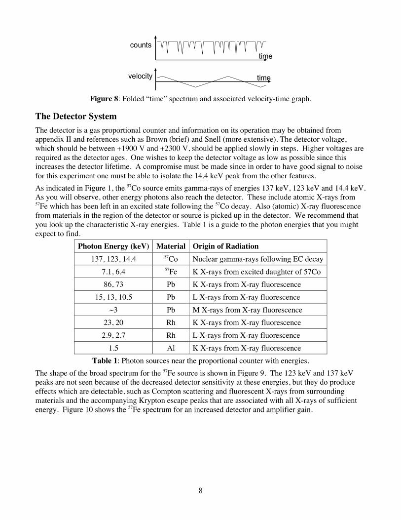
In this experiment the number of 14.4 keV gamma rays that pass through the absorber into a detector is measured as a function of the velocity of the source. The detector is a proportional counter that has been chosen since it efficiently detects the low energy gamma rays of interest but it is relatively insensitive to higher energy background gamma rays. To measure this spectrum, the 57Co source is moved backwards and forwards with a velocity that varies linearly as a function of time, while simultaneously multi-channel scaling is performed on the pulses (counts) coming from the detector. This produces a series of folded count versus time spectra from which counts versus velocity can be deduced. In multi-channel scaling, a number of bins or channels, each representing a time Δt, called the “dwell time”, record the counts as they come in. A “start” pulse starts the counting and if a pulse arrives, a count gets added to that bin that corresponds to the time delay for that pulse. (For example, if we set the dwell time to be 100 μs, and if a counter pulse arrives 20 ms after the start pulse, then one more count will be added to the “Channel 200” bin.) The source is mounted on a Mössbauer transducer which produces a velocity of motion proportional to the slow, highly linear, triangular voltage signal from the UCS Spectrometer Mössbauer output. The stationary absorber is a thin Fe foil. At liquid nitrogen temperatures there would be predominantly recoilless absorption, but even at room temperature about half the absorption events in 57Fe are recoilless and a reasonable spectrum can be obtained. The circuit hook-up for the apparatus is shown schematically in Figure 6 and a schematic section of the transducer is shown in Figure 7. Figure 8 illustrates the folded count versus time spectra.

7

PreAmpGain=x1

+ High VoltagePower Supply (2000V)

UCS 30 Spectrometer

Oscilloscope

Mössbauer Driver Mössbauer

Transducer

Spectroscopy Amplifier

Preamp Det Bias

Input

Out

put

CH 1

Velocit

y pick

-off to

CH 2

Proportional Counter

Computer with USX software

US

B

Figure 6: Schematic diagram of connections to the apparatus.

Figure 7: Schematic out view of the transducer.

8

counts

velocity

time

time

Figure 8: Folded “time” spectrum and associated velocity-time graph.

The Detector System The detector is a gas proportional counter and information on its operation may be obtained from appendix II and references such as Brown (brief) and Snell (more extensive). The detector voltage, which should be between +1900 V and +2300 V, should be applied slowly in steps. Higher voltages are required as the detector ages. One wishes to keep the detector voltage as low as possible since this increases the detector lifetime. A compromise must be made since in order to have good signal to noise for this experiment one must be able to isolate the 14.4 keV peak from the other features. As indicated in Figure 1, the 57Co source emits gamma-rays of energies 137 keV, 123 keV and 14.4 keV. As you will observe, other energy photons also reach the detector. These include atomic X-rays from 57Fe which has been left in an excited state following the 57Co decay. Also (atomic) X-ray fluorescence from materials in the region of the detector or source is picked up in the detector. We recommend that you look up the characteristic X-ray energies. Table 1 is a guide to the photon energies that you might expect to find.

Photon Energy (keV) Material Origin of Radiation 137, 123, 14.4 57Co Nuclear gamma-rays following EC decay

7.1, 6.4 57Fe K X-rays from excited daughter of 57Co 86, 73 Pb K X-rays from X-ray fluorescence

15, 13, 10.5 Pb L X-rays from X-ray fluorescence ~3 Pb M X-rays from X-ray fluorescence

23, 20 Rh K X-rays from X-ray fluorescence 2.9, 2.7 Rh L X-rays from X-ray fluorescence

1.5 Al K X-rays from X-ray fluorescence Table 1: Photon sources near the proportional counter with energies.

The shape of the broad spectrum for the 57Fe source is shown in Figure 9. The 123 keV and 137 keV peaks are not seen because of the decreased detector sensitivity at these energies, but they do produce effects which are detectable, such as Compton scattering and fluorescent X-rays from surrounding materials and the accompanying Krypton escape peaks that are associated with all X-rays of sufficient energy. Figure 10 shows the 57Fe spectrum for an increased detector and amplifier gain.

9

Figure 9: X-ray spectrum for low detector voltage and low amplifier gain.

Figure 10: X-ray spectrum for high detector voltage and high amplifier gain.

In order to not have the Mössbauer absorption overwhelmed by detection of non-resonant radiation energies, it is necessary to have the detector register only the 14.4 keV gamma-rays and not count those of other energy. (You might reflect on why all lead shielding in the apparatus is lined with aluminium.) The discrimination against unwanted photons uses the property of the detector that the pulses out of the proportional counter have heights (voltages) proportional to the photon energy. Moreover, the multi-channel scaler (MCS) of the UCS 30 has, at its front end, a single channel analyzer which accepts only a certain range of pulse heights. To set up the detector to select only the 14.4 keV gamma-rays:

1. The detector should feed the pre-amplifier and then the spectrometer. (The Spectrometer Amplifier is currently just used to provide power to the pre-amp, but it could be used between the pre-amp and spectrometer if more gain or better pulse-shaping were needed.) Start with a pre-amp gain of “×1”. Using the oscilloscope connected to the pre-amp output, you should be able to see pulses the detector. The largest pulses should be from the 137 keV gamma-rays. The pulses you are interested in, from the 14.4 keV gamma-rays, are the intense traces about 1/10 of the voltage of the highest ones.

2. Connect the pre-amp output to the spectrometer input. (For operation of the UCS-30, see the manual: http://www.spectrumtechniques.com/manuals/UCS30_Manual.pdf.) You will now take a pulse height spectrum to enable you to set the UCS-30 to respond to only pulses of height corresponding to the 14.4 keV gamma-ray energy. Using the USX software on the experiment’s computer, collect a pulse height spectrum. The display on the screen is a histogram of the distribution of pulse heights that you previously saw on the oscilloscope. You should be able to identify a number of the higher energy photons mentioned in Table 1. The 14.4 keV gamma-ray may or may not be visible – it may be at too low a voltage. The recommended method to

10

identify the endpoint of the spectrum corresponding to 137 KeV, which allows you to roughly identify where 14.4 KeV is, then to focus in around 14.4 KeV where the middle of three broad peaks should be the desired line. You may need to adjust the gain. You now set the “window” of the single channel analyzer (SCA) mode to include the whole peak and no more. (Note that the peak is broad as gas proportional counters have poor energy resolution.)

The Transducer The Mössbauer transducer, shown in Figure 7, provides a controlled motion of the source. It has two coils mounted to a common shaft which moves longitudinally. The coils sit in magnetic fields so that the field cuts the wires normally. The drive coil moves the shaft, providing a force proportional to the current through it. The pickup coil produces a voltage proportional to the velocity of the shaft. The Mössbauer Driver with the transducer is represented schematically in Figure 11.

Pickupcoil

Drivecoil

Velocitypick-off(to scope)

DifferenceAmplifier

WavetekFunctionGenerator

Source

functioninput

USB-30 Mössbauer Output (MSB OUT)

Figure 11: Functional schematic diagram of the Mössbauer driver and transducer.

The pickup coil output voltage is subtracted from the Function Input (derived from the USB-30) and then amplified. The amplified output is used to drive the drive coil. If the amplifier has sufficient gain, the feedback in this arrangement drives the shaft so as to make the pickup coil voltage follow the Function Input voltage. Thus the velocity of the shaft is proportional to the Function Input voltage. There are other features in the circuitry that help prevent the transducer shaft from wandering off too far past the ends of normal motion. The Velocity Pickoff enables you to display an actual velocity-time graph on the slow cathode ray oscilloscope.

Velocity Selection of the Source The internal magnetic field in the absorber produces the magnetic splitting of the nuclear levels and the transitions between the levels have energies which differ from the energy of the X-rays from the source. These energy differences are given in Figure 3 in terms of the velocity required to Doppler shift a 14.4 keV X-ray from the source to the appropriate energy to produce a transition. From Figure 3 it can be seen that the velocity must range from about −6 mm/s to +6 mm/s in order to see all the lines. The maximum velocity of the source is determined by its maximum amplitude and period. If, for a given velocity, the period is large, then the amplitude of the transducer must be correspondingly large. If the amplitude is too large then the transducer will be overdriven and this will give rise to glitches in the velocity profile as seen on the oscilloscope. On the other hand, if the amplitude is small, the period

11

will have to be short in order to give high enough velocities to perform this experiment. This will make visual observations of the amplitude using a travelling microscope very difficult. A reasonable compromise for the amplitude of the transducer is between 0.5 and 1 mm. A quick approximation to the amplitude of the source should be made using the dial gauge on the exposed free end of the transducer shaft, i.e. the end that one can see, opposite from the other inaccessible end with source attached. A rough approximation to the period may be taken from the oscilloscope or from the counter. Since the velocity changes linearly with time, then vmax may be calculated from tvd = where vv 2max = . Do not leave the dial gauge pushing against the exposed free end of the transducer shaft when taking data, since even the small extra force from the gauge can make the velocity profile nonlinear. Before taking data it can be useful to gently put one’s finger on the free end of the transducer shaft so that one can feel that the motion of the shaft is smooth.

Setting the Time Scales for Observation There are two time scales that you have to set: the Dwell Time and the period of the motion of the transducer. Use the Oscilloscope to determine the correlation between the UCS-30 MSB OUT signal and the observed position of the transducer. The entire range of velocities that you have selected will be swept through in a time equal to one half of the period of the transducer. Set an appropriate dwell time per channel so that the horizontal axis of the UCS-30 time spectrum corresponds to slightly longer than one half of the transducer period. In this way any pattern that appears will start to repeat and you will thus be able to determine the end point of the pattern. Start the acquisition of Mössbauer data. A very rough pattern of absorption peaks should start to appear after between about one to four hours, depending on the source strength. Running overnight is recommended to be sure that one is seeing – or not – the desired absorption peaks. It may be necessary to adjust the amplitude, frequency, and dwell time if the display if the observed spectrum is not similar to Figure 2. Remember that the display should be spread out as much as possible to give the best energy resolution but still have the last peak in the pattern repeated so that the end of the pattern may be determined. For fine adjustments it may be easier to select the dwell time first and then adjust the period of the transducer. The end point of the pattern is determined by selecting the midpoint between the “last” peak in the pattern and its repetition as the pattern starts to repeat. In the ideal situation channel 0 of the spectrometer spectrum should correspond to v = vmax.

Velocity Calibration of the Transducer A precise measurement of the amplitude of the motion should be made using the dial gauge. Release the spacer holding the dial gauge away from the end of the transducer and determine the total distance of travel of the transducer. Be sure to do this at the beginning and at the end of your run so that you can confirm that velocity conditions remained constant. The period may be measured precisely using the oscilloscope. Determine vmax

as before and hence determine the velocity increment per channel of the spectrum.

12

DATA COLLECTION AND ANALYSIS Collect data for a time long enough so that the resonance peaks are well defined. This may take as long as a day for a nice spectrum; you may wish to leave the apparatus running overnight or over a weekend. Stop acquisition of data and save it, both to the experiment computer and to a USB key or the cloud. It is recommended the file have a useful name that includes the date the data was taken. Analysis Notes:

1. Data analysis can be done by modifying curve_fit_to_data.py or other programs at http://www.physics.utoronto.ca/~phy326/python. The fitting function in these programs will need to be modified to include all the observed absorption peaks and the background.

2. An “absorption peak” is a dip in the spectrum. The fitting programs can easily handle such negative height peaks, so there is no need and much risk in trying to “invert” the data. You will need to decide whether fitting to Gaussian, Lorentzian, or some other shaped peaks are appropriate.

3. The background is not uniform, and in fact you can easily observe the 1/r2 variations in the background intensity as the source detector distance changes over the transducer cycle.

Question 4: Do these background variations agree with your measurements of the amplitude and period, and your previous determination the transducer position at the beginning of the spectrum. It may be helpful to take some pure background data by selecting a gamma energy region away from the 14.4 KeV absorption lines, in which case no dips should be observed in the background, only the gentle oscillations as the sources moves closer and farther from the detector.

Questions to consider when looking at your data: 1. Determine the widths and intensities of the peaks. (Does the intensity correspond to the height or

the area of the peak?) Are the widths equal and are their intensities in the ratio that you would expect? Make sure you calculate and include the uncertainties in all these quantities.

2. Note that the spacing between the peaks near vmax at the beginning of the pattern is not the same as the spacing between the peaks near vmax at the end of the pattern. Why not?

3. Which channels correspond to maximum velocity? They will be half-way between the pairs of large peaks at the beginning and at the end of the pattern.

4. Is there some symmetry to the pattern? If there is, the midpoints between corresponding peaks for positive and negative velocities will be the same.

13

Calculations and Conclusions The Mössbauer pattern for 57Fe obtained in this experiment can be looked at in terms of two perspectives; one primarily of nuclear physics and the other primarily of solid state physics. These are, however, still just different aspects of the one physical effect. Listed below are a number of determinations of physical quantities which can be made from the Mössbauer pattern data. You should respond to at least half of these in detail and be aware of the significance of the others.

I. Nuclear Physics Aspects 1. Calculate the lifetimes of the spectral states giving the Mössbauer lines and try to account for any

discrepancy between your results and what you might expect from you reading of the literature. 2. Confirm that the relative peak heights are what you would expect from your knowledge of the

nuclear decay scheme for the 14.4 keV gamma-ray from 57Fe.

II. Solid State Aspects 3. Calculate the isomer shift for your observed Mössbauer pattern and by referring to Figure 1, suggest

the identity of the element providing the matrix for the Mössbauer source. 4. Calculate the Mössbauer fraction for 57Fe at room temperature -- do not use a low temperature

approximation. 5. Assume that the value for the magnetic moment of the ground state µ1/2 is 0.09024 nuclear

magnetons (CRC Handbook) where the nuclear magneton µN = 5.0508 × 10-27 J/T. Calculate the magnetic hyperfine field at the 57Fe nucleus, giving the value in Tesla.

The Mössbauer effect is well displayed in iron and has been used effectively in a few other elements (eg. tin) and alloys, but it does not occur universally in an easily observed manner. For it to be readily observed in a given crystal, the following considerations must be favourable:

a. gamma-ray energy. b. Line width of the nuclear transition. c. The value of QD for the crystal. d. The degree of complexity of the nuclear transition.

Some parameters for iron are listed below, together with the experimentally determined phonon density of states.

Figure 12: Frequency Distribution for B.C.C. Iron and the Equivalent Debye Temperature Relation.

(Brockhouse et al, Solid State Communications 5, 211, 1967.)

14

REFERENCES 1. Brown, B. (1963) Experimental Nucleonics, Prentice Hall. (QC 784 B7) 2. Frauenfelder, H. (1962) The Mössbauer Effect, W.A. Benjamin, New York. (QC 490 F7,

available in APL, but DO NOT REMOVE.) 3. Gonser, U. (1975) From a Strange Effect to Mossbauer Spectroscopy, in Mossbauer

Spectroscopy 5 (1975) 1-51, Springer-Verlag Topics in Applied Physics. (http://link.springer.com.myaccess.library.utoronto.ca/chapter/10.1007/3540071202_13)

4. Harrison, W.A. (1970) Solid State Theory, McGraw-Hill. (QC 176 H27) 5. Lipkin, H.J. Some simple features of the Mössbauer effect, Annals of Physics 9 (1960) 332-339.

(http://www.sciencedirect.com.myaccess.library.utoronto.ca/science/article/pii/000349166090035X) 6. Mössbauer, R.L. Kernresonanzfluoreszenz von Gammastrahlung in Ir191, Z. Physik 151 (1958)

124-143. Later review paper: R.L. Mössbauer, Recoilless nuclear resonance absorption, Ann. Rev. Nuclear Sci. 12 (1962) 123 .

7. Preston, R.S., S.S. Hanna, & J. Heberle Mössbauer Effect in Metallic Iron, Physical Review 128 (1962) 2207-2218. (http://journals.aps.org/pr/pdf/10.1103/PhysRev.128.2207)

8. Sharma, V.K. (editors), G. Klingelhöfer, & T. Nishida (2014) Mössbauer Spectroscopy: Applications in Chemistry, Biology, and Nanotechnology, John Wiley & Sons. (http://onlinelibrary.wiley.com.myaccess.library.utoronto.ca/book/10.1002/9781118714614)

9. Snell, A.H. (1962) Nuclear Instruments and Their Uses, Vol. 1, John Wiley and Sons, (QC 786 N38)

10. Wertheim, G. K. (1964) Mössbauer Effect: Principles and applications. Academic Press, N.Y. (QC 490 W4)