Mortgage Innovation, Mortgage Choice, and Housing Decisions · Mortgage Innovation, Mortgage...

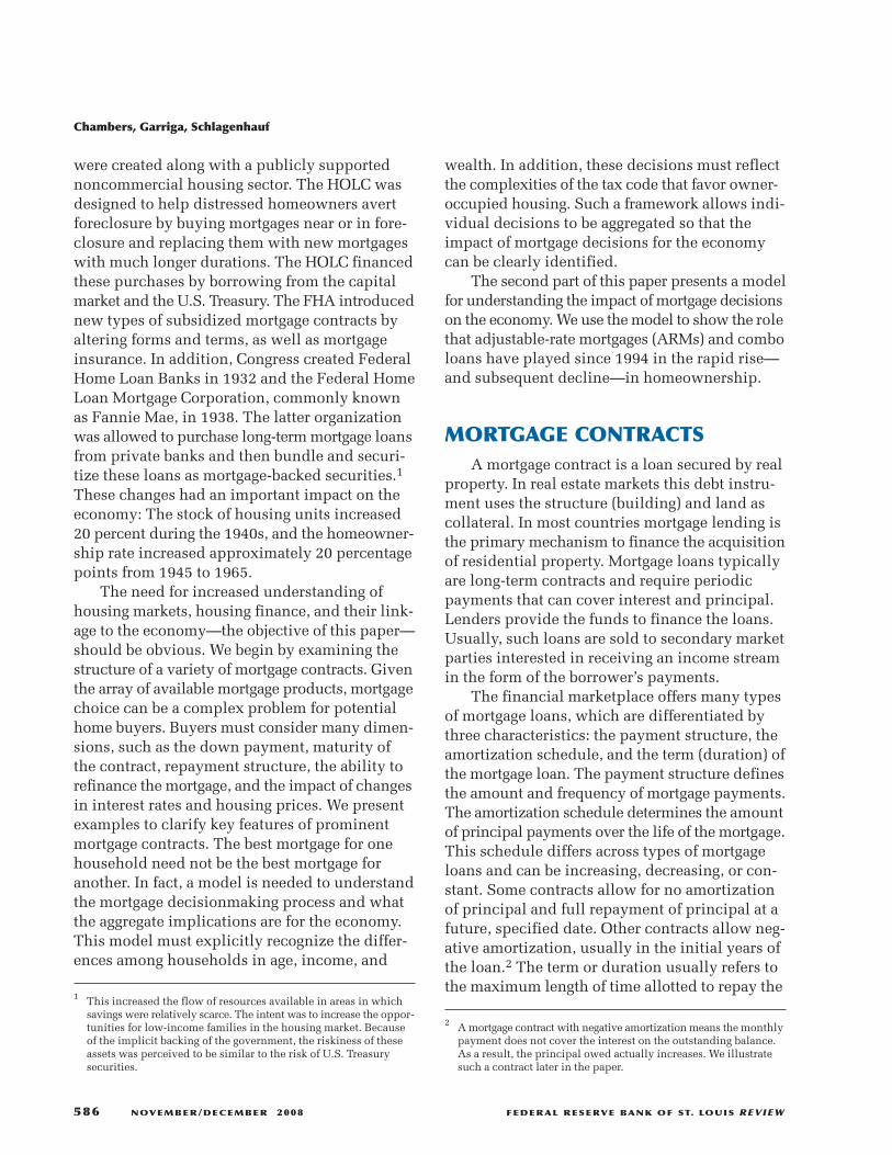
FEDERAL RESERVE BANK OF ST. LOUIS REVIEW NOVEMBER/DECEMBER 2008 585

Mortgage Innovation, Mortgage Choice, and Housing Decisions

Matthew S. Chambers, Carlos Garriga, and Don Schlagenhauf

This paper examines some of the more recent mortgage products now available to borrowers.The authors describe how these products differ across important characteristics, such as the downpayment requirement, repayment structure, and amortization schedule. The paper also presents amodel with the potential to analyze the implications for various mortgage contracts for individualhouseholds, as well as to address many current housing market issues. In this paper, the authorsuse the model to examine the implications of alternative mortgages for homeownership. The authorsuse the model to show that interest rate–adjustable mortgages and combo loans can help explainthe rise—and fall—in homeownership since 1994. (JEL E2, E6)

Federal Reserve Bank of St. Louis Review, November/December 2008, 90(6), 585-608.

foreclosures has again focused attention on theimportance of housing. Fears have increased thatmortgage market problems will have long-lastingeffects on the credit market and thus continue tocreate a drag on the economy.

Events illustrating the important role ofhousing in the economy are not limited to thoseof the past decade. Housing foreclosures soaredduring the Great Depression as a result of twofactors. The mortgage system was very restrictive:Homeowners were required to make down pay-ments that averaged around 35 percent for loanslasting only five to ten years. At the end of theloan period, mortgage holders had to either payoff the loan or find new financing. The 1929 stockmarket collapse resulted in numerous bank fail-ures. Mortgage issuance fell drastically, and home-owners were dragged into foreclosure. Faced withthese problems, the government developed newhousing policies as part of the New Deal legisla-tion. The Home Owners’ Loan Corporation (HOLC)and the Federal Housing Administration (FHA)

H ousing is a big-ticket item in theU.S. economy. At the macro level,residential housing investmentaccounts for 20 to 25 percent of

gross private investment. In the aggregate, thisfinancing is about 8 trillion dollars and uses asizable fraction of the financial resources of theeconomy. The importance of housing at the indi-vidual household level is more evident becausethe purchase of a house is the largest single con-sumer transaction and nearly always requiresmortgage financing. This decision affects theoverall expenditure patterns and asset allocationdecisions of the household.

In recent years, interest in the role of housingin the U.S. economy has increased, influencedmainly by two events. During the economicdownturn in 2000, the housing sector seemed tomitigate the slowdown in many other sectors ofthe economy as residential investment remainedat high levels. More recently, the large number of

Matthew S. Chambers is an assistant professor of economics at Towson University. Carlos Garriga is an economist at the Federal Reserve Bankof St. Louis. Don Schlagenhauf is a professor of economics at Florida State University. The authors are grateful for the financial support ofthe National Science Foundation (grant No. SEP-0649374). Carlos Garriga also acknowledges support from the Spanish Ministry of Scienceand Technology (grant No. SEJ2006-02879). Michelle T. Armesto provided research assistance.

© 2008, The Federal Reserve Bank of St. Louis. The views expressed in this article are those of the author(s) and do not necessarily reflect theviews of the Federal Reserve System, the Board of Governors, or the regional Federal Reserve Banks. Articles may be reprinted, reproduced,published, distributed, displayed, and transmitted in their entirety if copyright notice, author name(s), and full citation are included. Abstracts,synopses, and other derivative works may be made only with prior written permission of the Federal Reserve Bank of St. Louis.

were created along with a publicly supportednoncommercial housing sector. The HOLC wasdesigned to help distressed homeowners avertforeclosure by buying mortgages near or in fore-closure and replacing them with new mortgageswith much longer durations. The HOLC financedthese purchases by borrowing from the capitalmarket and the U.S. Treasury. The FHA introducednew types of subsidized mortgage contracts byaltering forms and terms, as well as mortgageinsurance. In addition, Congress created FederalHome Loan Banks in 1932 and the Federal HomeLoan Mortgage Corporation, commonly knownas Fannie Mae, in 1938. The latter organizationwas allowed to purchase long-term mortgage loansfrom private banks and then bundle and securi-tize these loans as mortgage-backed securities.1

These changes had an important impact on theeconomy: The stock of housing units increased20 percent during the 1940s, and the homeowner-ship rate increased approximately 20 percentagepoints from 1945 to 1965.

The need for increased understanding ofhousing markets, housing finance, and their link-age to the economy—the objective of this paper—should be obvious. We begin by examining thestructure of a variety of mortgage contracts. Giventhe array of available mortgage products, mortgagechoice can be a complex problem for potentialhome buyers. Buyers must consider many dimen-sions, such as the down payment, maturity ofthe contract, repayment structure, the ability torefinance the mortgage, and the impact of changesin interest rates and housing prices. We presentexamples to clarify key features of prominentmortgage contracts. The best mortgage for onehousehold need not be the best mortgage foranother. In fact, a model is needed to understandthe mortgage decisionmaking process and whatthe aggregate implications are for the economy.This model must explicitly recognize the differ-ences among households in age, income, and

wealth. In addition, these decisions must reflectthe complexities of the tax code that favor owner-occupied housing. Such a framework allows indi-vidual decisions to be aggregated so that theimpact of mortgage decisions for the economycan be clearly identified.

The second part of this paper presents a modelfor understanding the impact of mortgage decisionson the economy. We use the model to show the rolethat adjustable-rate mortgages (ARMs) and comboloans have played since 1994 in the rapid rise—and subsequent decline—in homeownership.

MORTGAGE CONTRACTSA mortgage contract is a loan secured by real

property. In real estate markets this debt instru-ment uses the structure (building) and land ascollateral. In most countries mortgage lending isthe primary mechanism to finance the acquisitionof residential property. Mortgage loans typicallyare long-term contracts and require periodicpayments that can cover interest and principal.Lenders provide the funds to finance the loans.Usually, such loans are sold to secondary marketparties interested in receiving an income streamin the form of the borrower’s payments.

The financial marketplace offers many typesof mortgage loans, which are differentiated bythree characteristics: the payment structure, theamortization schedule, and the term (duration) ofthe mortgage loan. The payment structure definesthe amount and frequency of mortgage payments.The amortization schedule determines the amountof principal payments over the life of the mortgage.This schedule differs across types of mortgageloans and can be increasing, decreasing, or con-stant. Some contracts allow for no amortizationof principal and full repayment of principal at afuture, specified date. Other contracts allow neg-ative amortization, usually in the initial years ofthe loan.2 The term or duration usually refers tothe maximum length of time allotted to repay the

Chambers, Garriga, Schlagenhauf

586 NOVEMBER/DECEMBER 2008 FEDERAL RESERVE BANK OF ST. LOUIS REVIEW

1 This increased the flow of resources available in areas in whichsavings were relatively scarce. The intent was to increase the oppor-tunities for low-income families in the housing market. Becauseof the implicit backing of the government, the riskiness of theseassets was perceived to be similar to the risk of U.S. Treasurysecurities.

2 A mortgage contract with negative amortization means the monthlypayment does not cover the interest on the outstanding balance.As a result, the principal owed actually increases. We illustratesuch a contract later in the paper.

mortgage loan. The most common mortgage con-tracts are for 15 and 30 years. The combinationof these three factors allows a large variety ofdistinct mortgage products.

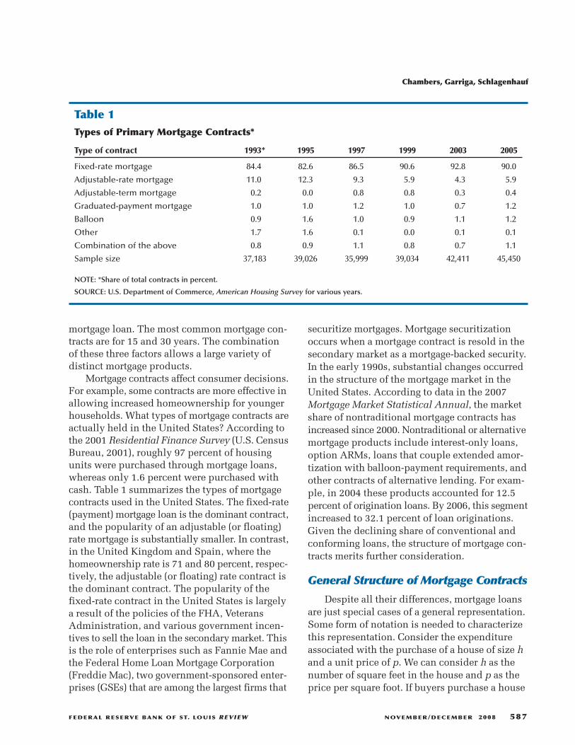
Mortgage contracts affect consumer decisions.For example, some contracts are more effective inallowing increased homeownership for youngerhouseholds. What types of mortgage contracts areactually held in the United States? According tothe 2001 Residential Finance Survey (U.S. CensusBureau, 2001), roughly 97 percent of housingunits were purchased through mortgage loans,whereas only 1.6 percent were purchased withcash. Table 1 summarizes the types of mortgagecontracts used in the United States. The fixed-rate(payment) mortgage loan is the dominant contract,and the popularity of an adjustable (or floating)rate mortgage is substantially smaller. In contrast,in the United Kingdom and Spain, where thehomeownership rate is 71 and 80 percent, respec-tively, the adjustable (or floating) rate contract isthe dominant contract. The popularity of thefixed-rate contract in the United States is largelya result of the policies of the FHA, VeteransAdministration, and various government incen-tives to sell the loan in the secondary market. Thisis the role of enterprises such as Fannie Mae andthe Federal Home Loan Mortgage Corporation(Freddie Mac), two government-sponsored enter-prises (GSEs) that are among the largest firms that

securitize mortgages. Mortgage securitizationoccurs when a mortgage contract is resold in thesecondary market as a mortgage-backed security.In the early 1990s, substantial changes occurredin the structure of the mortgage market in theUnited States. According to data in the 2007Mortgage Market Statistical Annual, the marketshare of nontraditional mortgage contracts hasincreased since 2000. Nontraditional or alternativemortgage products include interest-only loans,option ARMs, loans that couple extended amor-tization with balloon-payment requirements, andother contracts of alternative lending. For exam-ple, in 2004 these products accounted for 12.5percent of origination loans. By 2006, this segmentincreased to 32.1 percent of loan originations.Given the declining share of conventional andconforming loans, the structure of mortgage con-tracts merits further consideration.

General Structure of Mortgage Contracts

Despite all their differences, mortgage loansare just special cases of a general representation.Some form of notation is needed to characterizethis representation. Consider the expenditureassociated with the purchase of a house of size hand a unit price of p. We can consider h as thenumber of square feet in the house and p as theprice per square foot. If buyers purchase a house



Table 1Types of Primary Mortgage Contracts*

Type of contract 1993* 1995 1997 1999 2003 2005

Fixed-rate mortgage 84.4 82.6 86.5 90.6 92.8 90.0

Adjustable-rate mortgage 11.0 12.3 9.3 5.9 4.3 5.9

Adjustable-term mortgage 0.2 0.0 0.8 0.8 0.3 0.4

Graduated-payment mortgage 1.0 1.0 1.2 1.0 0.7 1.2

Balloon 0.9 1.6 1.0 0.9 1.1 1.2

Other 1.7 1.6 0.1 0.0 0.1 0.1

Combination of the above 0.8 0.9 1.1 0.8 0.7 1.1

Sample size 37,183 39,026 35,999 39,034 42,411 45,450

NOTE: *Share of total contracts in percent.

SOURCE: U.S. Department of Commerce, American Housing Survey for various years.

with cash, the total expenditure is then denotedby ph. Most buyers do not have assets availablethat allow a check to be written for ph, and there-fore they must acquire a loan to finance this largeexpenditure.

In general, a mortgage loan requires a downpayment equal to χ percent of the value of thehouse. The amount χph represents the amountof equity in the house at the time of purchase,and D0 = �1 – χ�ph represents the initial amountof the loan. In a particular period, denoted by n,the borrower faces a payment amount mn (i.e.,monthly or yearly payment) that depends on thesize of the original loan, D0, the length of the mort-gage, N, and the mortgage interest rate, rm. Thispayment can be subdivided into an amortization(or principal) component, An, which is determinedby the amortization schedule, and an interestcomponent, In, which depends on the paymentschedule. That is,

(1)

where the interest payments are calculated by In = r

mDn.3 An expression that determines howthe remaining debt, Dn, changes over time can bewritten as

(2)

This formula shows that the level of outstandingdebt at the start of period n is reduced by theamount of any principal payment. A principalpayment increases the level of equity in the home.If the amount of equity in a home at the start ofperiod n is defined as Hn, a payment of principalequal to An increases equity in the house availablein the next period to Hn+1. Formally,

(3)

where H0 = χph denotes the home equity in theinitial period.4

This representation of mortgage contracts isvery general and summarizes many of the differ-

m A I nn n n= + ∀, ,� �

D D A nn n n+ = − ∀1 , .� �

H H A nn n n+ = + ∀1 , ,

ent contracts available in the financial markets.For example, this formulation can accommodatea no-down-payment loan by setting χ = 0 so thatthe initial loan is equal to D0 = ph. Because thisframework can be used to characterize differencesin the amortization terms and payment schedules,we use it to describe the characteristics of someprominent types of mortgage loans.

Mortgage Loans with Constant Payments

In the United States, fixed-rate mortgages(FRMs) typically are considered the standard mort-gage contract. This loan product is characterizedby a constant mortgage payment over the term ofthe mortgage, m � m1 = … = mN. This value, m,must be consistent with the condition that thepresent value of mortgage payments repays theinitial loan. That is,

If this equation is solved for m, we can write

where λ = rm[1 – �1 + rm�–N]–1. Because the mort-gage payment is constant each period, and m =At + It, the outstanding debt decreases over timeD0 > … > Dn. This means the fixed-payment con-tract front-loads interest rate payments,

and, thus, back-loads principal payments,

The equity in the house increases each period bythe mortgage payment net of the interest paymentcomponent:

We now present some examples to illustrate keyproperties of the FRM contract.

D phm

rm

r

m

rN N0 11 1 1≡ =

++ +

+( )+

+( )−χ .

m D= λ 0,

D r D m nnm

n+ = +( ) − ∀1 1 , ,

A m r Dnm

n= − .

H H m r D nn nm

n+ = + − ∀1 , .

3 The calculation of the mortgage payment depends on the charac-teristics of the contract, but for all contracts the present value ofthe payments must be equal to the total amount borrowed,

D phm

r

m

r

m

rN

N01 2

21 1 1

≡ =+

++( )

+ ++( )

χ .



4 It is important to state that for the sake of simplicity this frame-work assumes no changes in house prices. If house prices areallowed to change, then the equity equation would have to allowfor capital gains and losses.

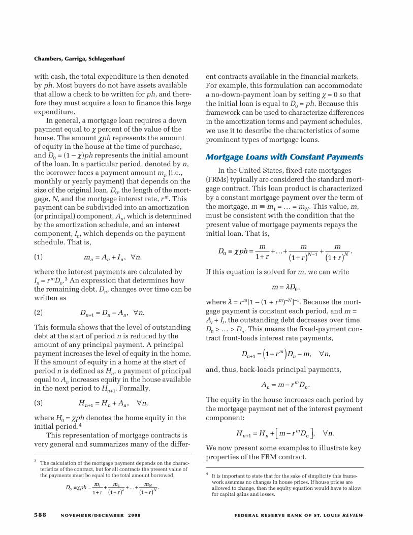
Example 1. Consider the purchase of a housewith a total cost of ph = $250,000 using a loanwith a 20 percent down payment, χ = 0.20; aninterest rate of 6 percent annually; and a 30-yearmaturity. This mortgage loan is for $200,000.5

Table 2 illustrates the changes in interest andprincipal payments per month over the lengthof the mortgage contract.

The first two rows of Table 2 show the mort-gage payment in the first and second months ofthe contract. The monthly payment on this mort-gage is $1,178.74. In the first period, $973.51 ofthe monthly payment goes to interest rate pay-ments. This means the principal payment is only$205.23.6 Now, let us consider the mortgage pay-ment 10 years into the mortgage. Although themonthly payment does not change, the principalpayment has increased to $365.76 and the interestpayment component has decreased to $812.98.After 10 years, the homeowner has paid off only

$33,344.41 of the original $200,000 loan. Themonth after the halfway point in the mortgageoccurs at period 181. The interest payment com-ponent of the monthly payment still exceeds theprincipal payment. In payment period 219—18years and 3 months into the contract—the prin-cipal component of the monthly payment finallyexceeds the interest payment component. Fromthis point forward, the principal payment will belarger than the interest payment. At the end of20 years, or period 240, the principal componentof the $1,178.74 monthly payment is $655.01.However, $106,941.84 is still owed on the original$200,000 loan. The outstanding loan balance doesnot drop below $100,000 until payment period251. With a standard 30-year mortgage contract,it takes nearly 22 years to pay off half the mortgageloan. The remaining half of the mortgage will berepaid in the final 8 years of this mortgage.

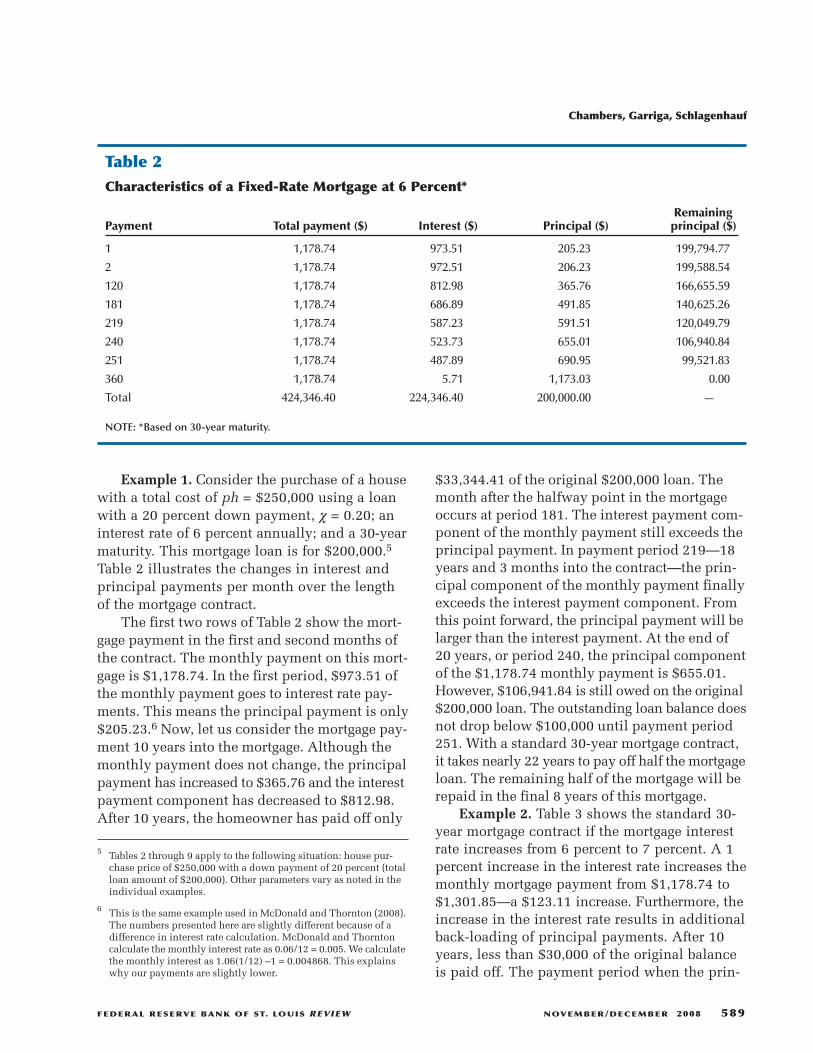
Example 2. Table 3 shows the standard 30-year mortgage contract if the mortgage interestrate increases from 6 percent to 7 percent. A 1percent increase in the interest rate increases themonthly mortgage payment from $1,178.74 to$1,301.85—a $123.11 increase. Furthermore, theincrease in the interest rate results in additionalback-loading of principal payments. After 10years, less than $30,000 of the original balanceis paid off. The payment period when the prin-



5 Tables 2 through 9 apply to the following situation: house pur-chase price of $250,000 with a down payment of 20 percent (totalloan amount of $200,000). Other parameters vary as noted in theindividual examples.

6 This is the same example used in McDonald and Thornton (2008).The numbers presented here are slightly different because of adifference in interest rate calculation. McDonald and Thorntoncalculate the monthly interest rate as 0.06/12 = 0.005. We calculatethe monthly interest as 1.06�1/12� –1 = 0.004868. This explainswhy our payments are slightly lower.

Table 2Characteristics of a Fixed-Rate Mortgage at 6 Percent*

Remaining Payment Total payment ($) Interest ($) Principal ($) principal ($)

1 1,178.74 973.51 205.23 199,794.77

2 1,178.74 972.51 206.23 199,588.54

120 1,178.74 812.98 365.76 166,655.59

181 1,178.74 686.89 491.85 140,625.26

219 1,178.74 587.23 591.51 120,049.79

240 1,178.74 523.73 655.01 106,940.84

251 1,178.74 487.89 690.95 99,521.83

360 1,178.74 5.71 1,173.03 0.00

Total 424,346.40 224,346.40 200,000.00 —

NOTE: *Based on 30-year maturity.

cipal component exceeds the interest componentdoes not occur until period 239. In fact, the out-standing balance will not drop below $100,000until payment 260—9 months later than if theinterest rate is 6 percent (as in Example 1).

This table clearly illustrates the impact ofinterest rate changes on a mortgage loan. If thetotal interest payments on the mortgage contractpresented in Table 2 are compared with those inTable 3, the 1 percent increase in the interest rateresults in $44,320 of additional mortgage pay-ments over the life of the mortgage.

Mortgage with Constant Amortization

As seen in Tables 2 and 3, the FRM accrueslittle equity in the initial years of the mortgagebecause most of the mortgage payment servicesinterest payments. Some buyers would benefitby a combination of an FRM and faster equityaccrual. Can a mortgage contract be designed toallow accrual of more equity in the initial periods,and what properties would be involved in sucha contract? A mortgage contract with this benefitis known as a constant amortization mortgage(CAM). This loan contract allows constant con-tributions toward equity in each constant amorti-zation mortgage period; that is, the amortizationschedule is An = An+1 = A. Because the interest

repayment schedule depends on the size of out-standing level of debt, Dn, and the loan term, N,the mortgage payment, mn, is no longer constantover the duration of the loan. Formally, the con-stant amortization term is calculated by

If the expression for the interest payments isused, the monthly mortgage payment, mn, willdecrease over the length of the mortgage. Thischaracteristic of the CAM follows from the declinein outstanding principal over the life of the con-tract. The monthly payment is determined by

For this contract, the changes in the outstandinglevel of debt and home equity are represented by

and

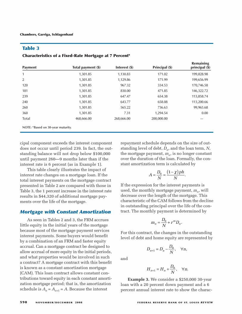
Example 3. We consider a $250,000 30-yearloan with a 20 percent down payment and a 6percent annual interest rate to show the charac-

ADN

phN

= =−( )0 1 χ

.

mDN

r Dnm

n= +0 .

D DDN

nn n+ = − ∀10 , ,

H HDN

nn n+ = + ∀10 , .



Table 3Characteristics of a Fixed-Rate Mortgage at 7 Percent*


1 1,301.85 1,130.83 171.02 199,828.98

2 1,301.85 1,129.86 171.99 199,656.99

120 1,301.85 967.32 334.53 170,746.58

181 1,301.85 830.00 471.85 146,322.72

239 1,301.85 647.47 654.38 113,858.74

240 1,301.85 643.77 658.08 113,200.66

260 1,301.85 565.22 736.63 99,965.68

360 1,301.85 7.31 1,294.54 0.00

Total 468,666.00 268,666.00 200,000.00 —


teristics of this type of contract. Table 4 presentsthe monthly mortgage payment, principal com-ponent, and interest component.

The monthly payment with this contract hasa much different profile than that of a fixed-pay-ment mortgage loan. Clearly, the amount of themortgage payment declines over the life of theloan. The initial payment is nearly three timesthe size of the payment in the last period. Princi -pal payments are constant over the life of the loan,thus allowing for faster equity accumulation. Halfof the original principal is repaid halfway throughthe loan. From a wealth accumulation perspective,this is an attractive feature. However, the declin-ing payment profile is not positively correlatedwith a normal household’s earning pattern duringthe first half of the life cycle: Mortgage paymentsare highest when earnings tend to be lower. Froma household budget perspective, this could be avery unattractive option.

Balloon and Interest-Only Loans

The key property of the CAM is the paymentof principal every period. In contrast, balloonand interest-only loans allow no amortization ofprincipal throughout the term of the mortgage. Aballoon loan is a very simple contract in whichthe entire principal borrowed is paid in full inthe last payment period, N. This product tendsto be more popular when mortgage rates are high

and home buyers anticipate lower future mortgagerates. In addition, homeowners who expect to stayin their homes only for a short time may find thiscontract attractive as they are not concerned aboutpaying principal. The amortization schedule forthis contract can be written as

This means that the mortgage payment in allperiods, except the last period, is equal to theinterest rate payment, In = r

mD0. Hence, the mort-gage payment for this contract can be specified as

where D0 = �1 – χ�ph. The evolution of the out-standing level of debt can be written as

With an interest-only loan and no change inhouse prices, the homeowner never accrues equitybeyond the initial down payment. Hence, An = 0and mn = In = r

mD0 for all n. In essence, the home-owner effectively rents the property from thelender and the mortgage (interest) payments arethe effective rental cost. As a result, the monthly

An N

ph n Nn =∀ <

−( ) =

0

1

� � � �χ

.

mI n N

r D n Nn

n

m=∀ <

+( ) =

� � � �

1 0

,

DD n N

n Nnn

+ =∀ <

=

1 0

,

,.



Table 4Characteristics of a Constant Amortization Mortgage at 6 Percent*


1 1,529.07 973.51 555.56 199,444.44

2 1,526.36 970.81 555.56 198,888.89

120 1,207.27 651.71 555.56 133,333.33

156 1,109.92 554.36 555.56 113,333.33

181 1,042.31 486.76 555.56 99,444.44

240 882.76 327.21 555.56 66,666.67

360 558.26 2.70 555.56 0.00

Total 375,718.58 175,718.58 200,000.00 —


mortgage payment is minimized because no peri-odic payments toward equity are made. A home-owner is fully leveraged with the bank with thistype of mortgage contract. If capital gains arerealized, the return on the housing investment ismaximized. If the homeowner itemizes tax deduc-tions, a large interest deduction is an attractiveby-product of this contract.

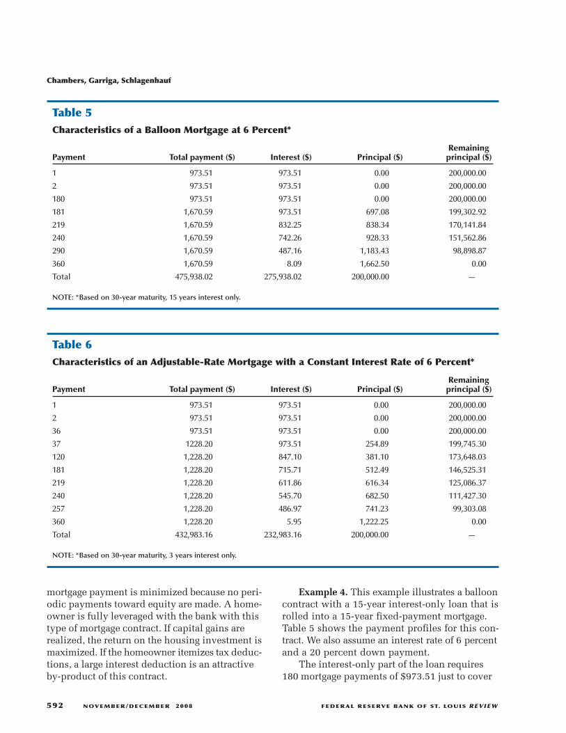
Example 4. This example illustrates a ballooncontract with a 15-year interest-only loan that isrolled into a 15-year fixed-payment mortgage.Table 5 shows the payment profiles for this con-tract. We also assume an interest rate of 6 percentand a 20 percent down payment.

The interest-only part of the loan requires180 mortgage payments of $973.51 just to cover



Table 5Characteristics of a Balloon Mortgage at 6 Percent*


1 973.51 973.51 0.00 200,000.00

2 973.51 973.51 0.00 200,000.00

180 973.51 973.51 0.00 200,000.00

181 1,670.59 973.51 697.08 199,302.92

219 1,670.59 832.25 838.34 170,141.84

240 1,670.59 742.26 928.33 151,562.86

290 1,670.59 487.16 1,183.43 98,898.87

360 1,670.59 8.09 1,662.50 0.00

Total 475,938.02 275,938.02 200,000.00 —

NOTE: *Based on 30-year maturity, 15 years interest only.

Table 6Characteristics of an Adjustable-Rate Mortgage with a Constant Interest Rate of 6 Percent*


1 973.51 973.51 0.00 200,000.00

2 973.51 973.51 0.00 200,000.00

36 973.51 973.51 0.00 200,000.00

37 1228.20 973.51 254.89 199,745.30

120 1,228.20 847.10 381.10 173,648.03

181 1,228.20 715.71 512.49 146,525.31

219 1,228.20 611.86 616.34 125,086.37

240 1,228.20 545.70 682.50 111,427.30

257 1,228.20 486.97 741.23 99,303.08

360 1,228.20 5.95 1,222.25 0.00

Total 432,983.16 232,983.16 200,000.00 —

NOTE: *Based on 30-year maturity, 3 years interest only.

the interest obligations on the $200,000 loan.After 15 years, the mortgage payment increasesto $1,670.59 because the 15-year balloon loan isrolled into a 15-year FRM. Payment number 219denotes the month in which principal paymentsexceed interest payments. In period 290, half ofthe $200,000 debt will be paid off. With this typeof mortgage contract, it takes more than 24 yearsto accrue $100,000 in equity.

Example 5. Some ARMs used in recent yearshave a very short period of interest-only pay-ments. Table 6 presents the payment profiles fora 3-year interest-only ARM that rolls into a 27-year standard FRM. The assumptions for theinterest rate, total contract length, and downpayment remain unchanged.

The monthly interest payments for thisinterest-only ARM are $973.51. Once the standard27-year contract takes effect, the monthly mort-gage payment increases by $254.69 to $1,228.20.This increase is not caused by an interest rateincrease, but rather payment toward principal.

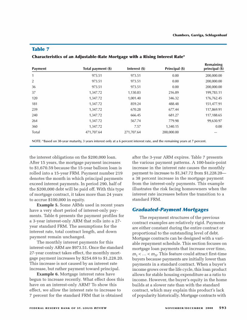
Example 6. Mortgage interest rates havebegun to increase recently. What effect does thishave on an interest-only ARM? To show thiseffect, we allow the interest rate to increase to7 percent for the standard FRM that is obtained

after the 3-year ARM expires. Table 7 presentsthe various payment patterns. A 100-basis-pointincrease in the interest rate causes the monthlypayment to increase to $1,347.72 from $1,228.20—a 38 percent increase in the mortgage paymentfrom the interest-only payments. This exampleillustrates the risk facing homeowners when theinterest rate increases before the transition to astandard FRM.

Graduated-Payment Mortgages

The repayment structures of the previouscontract examples are relatively rigid. Paymentsare either constant during the entire contract orproportional to the outstanding level of debt.Mortgage contracts can be designed with a vari-able repayment schedule. This section focuses onmortgage loan payments that increase over time,m1 < … < mN. This feature could attract first-timebuyers because payments are initially lower thanpayments in a standard contract. When a buyer’sincome grows over the life cycle, this loan productallows for stable housing expenditure as a ratio toincome. However, the buyer’s equity in the homebuilds at a slower rate than with the standardcontract, which may explain this product’s lackof popularity historically. Mortgage contracts with



Table 7Characteristics of an Adjustable-Rate Mortgage with a Rising Interest Rate*


1 973.51 973.51 0.00 200,000.00

2 973.51 973.51 0.00 200,000.00

36 973.51 973.51 0.00 200,000.00

37 1,347.72 1,130.83 216.89 199,783.11

120 1,347.72 1,001.40 346.32 176,762.45

181 1,347.72 859.24 488.48 151,477.91

239 1,347.72 670.28 677.44 117,869.91

240 1,347.72 666.45 681.27 117,188.65

264 1,347.72 567.74 779.98 99,630.97

360 1,347.72 7.57 1,340.15 0.00

Total 471,707.64 271,707.64 200,000.00 —

NOTE: *Based on 30-year maturity, 3 years interest only at a 6 percent interest rate, and the remaining years at 7 percent.

variable repayment schedules are known asgraduated-payment mortgages (GPMs). Thesecontracts are of special interest because theirfeatures are similar to those of mortgage contractssold to subprime borrowers.

The repayment schedule for a GPM dependson the growth rate of these payments. The growthrate of payments is specified in the mortgage con-tract, and borrowers considering this contractmust know this condition. We present examplesto illustrate why knowledge of this parameter orcondition is important. Typical GPM growth pat-terns are either geometric or arithmetic. We focuson GPMs with geometric growth patterns.

With this type of contract, mortgage paymentsevolve according to a constant geometric growthrate denoted by

where g > 0. This means the amortization andinterest payments also increase as

The initial mortgage payment is determined by

where λg = �rm – g�[1 – �1 + rm�–N]–1. The law ofmotion for the outstanding debt satisfies

m g mn n+ = +( )1 1 ,

m A In n n= + .

m Dg0 0= λ ,

and the amortization term is An = λgD0 – rmDn.

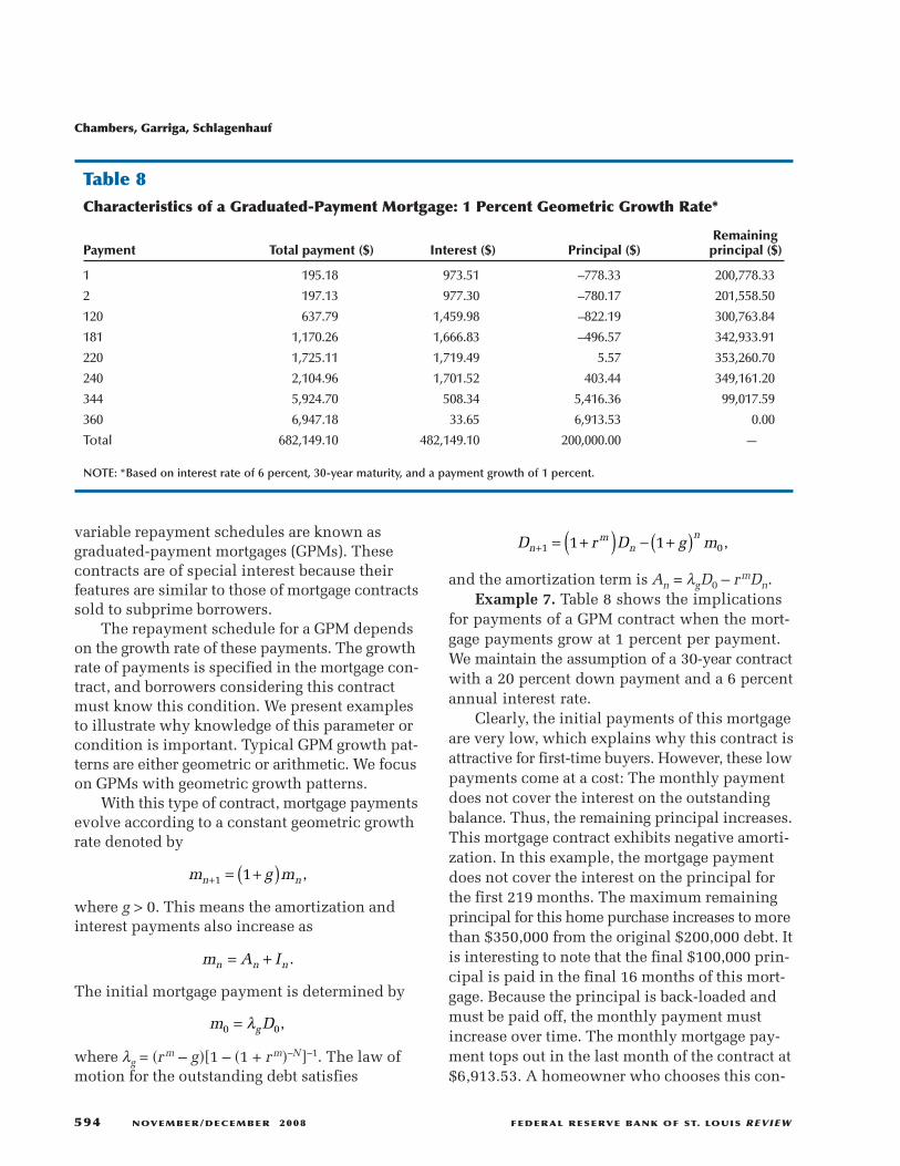
Example 7. Table 8 shows the implicationsfor payments of a GPM contract when the mort-gage payments grow at 1 percent per payment.We maintain the assumption of a 30-year contractwith a 20 percent down payment and a 6 percentannual interest rate.

Clearly, the initial payments of this mortgageare very low, which explains why this contract isattractive for first-time buyers. However, these lowpayments come at a cost: The monthly paymentdoes not cover the interest on the outstandingbalance. Thus, the remaining principal increases.This mortgage contract exhibits negative amorti-zation. In this example, the mortgage paymentdoes not cover the interest on the principal forthe first 219 months. The maximum remainingprincipal for this home purchase increases to morethan $350,000 from the original $200,000 debt. Itis interesting to note that the final $100,000 prin-cipal is paid in the final 16 months of this mort-gage. Because the principal is back-loaded andmust be paid off, the monthly payment mustincrease over time. The monthly mortgage pay-ment tops out in the last month of the contract at$6,913.53. A homeowner who chooses this con-

D r D g mnm

nn

+ = +( ) − +( )1 01 1 ,



Table 8Characteristics of a Graduated-Payment Mortgage: 1 Percent Geometric Growth Rate*


1 195.18 973.51 –778.33 200,778.33

2 197.13 977.30 –780.17 201,558.50

120 637.79 1,459.98 –822.19 300,763.84

181 1,170.26 1,666.83 –496.57 342,933.91

220 1,725.11 1,719.49 5.57 353,260.70

240 2,104.96 1,701.52 403.44 349,161.20

344 5,924.70 508.34 5,416.36 99,017.59

360 6,947.18 33.65 6,913.53 0.00

Total 682,149.10 482,149.10 200,000.00 —

NOTE: *Based on interest rate of 6 percent, 30-year maturity, and a payment growth of 1 percent.

tract pays $482,149.10 in total interest payments.Compared with the FRM contract presented inTable 2, total interest payments are more thandouble. These characteristics make GPMs riskyfrom a lender’s perspective because the potentialfor default is greater, which is one reason thistype of contract has not historically been a factorin the mortgage market.

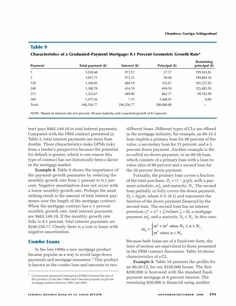
Example 8. Table 9 shows the importance ofthe payment growth parameter by reducing themonthly growth rate from 1 percent to 0.1 per-cent. Negative amortization does not occur witha lower monthly growth rate. Perhaps the moststriking result is the amount of total interest pay-ments over the length of the mortgage contract.When the mortgage contract has a 1 percentmonthly growth rate, total interest paymentsare $482,149.10. If the monthly growth ratefalls to 0.1 percent, total interest payments are$246,356.77. Clearly there is a cost to loans withnegative amortization.

Combo Loans

In the late 1990s a new mortgage productbecame popular as a way to avoid large downpayments and mortgage insurance.7 This productis known as the combo loan and amounts to two

different loans. Different types of CLs are offeredin the mortgage industry; for example, an 80-15-5loan implies a primary loan for 80 percent of thevalue, a secondary loan for 15 percent, and a 5percent down payment. Another example is theso-called no-down-payment, or an 80-20 loan,which consists of a primary loan with a loan-to-value ratio of 80 percent and a second loan forthe 20 percent down payment.

Formally, the primary loan covers a fractionof the total purchase, D1 = �1 – χ�ph, with a pay-ment schedule, m1

n, and maturity, N1. The secondloan partially or fully covers the down payment,D2 = ϑχph, where ϑ � �0,1] and represents thefraction of the down payment financed by thesecond loan. The second loan has an interestpremium r2

m = r1m + ζ (where ζ > 0), a mortgage

payment mn2, and a maturity N2 ≤ N1. In this case,

Because both loans are of a fixed-rate form, thelaws of motion are equivalent to those presentedin the FRM contract discussion. Table 10 showscharacteristics of a CL.

Example 9. Table 10 presents the profile foran 80-20 CL for our $250,000 house. The first$200,000 is borrowed with the standard fixed-payment mortgage at 6 percent interest. Theremaining $50,000 is financed using another

mm m N n N

m n Nn =

+ ≤ ≤

<

1 22 1

12

Ä Ä

Ä Ä.

when

when



7 Government-sponsored enterprises (GSEs) initiated the use ofthis product in the late 1990s and it became popular in privatemortgage markets between 2001 and 2002.

Table 9Characteristics of a Graduated-Payment Mortgage: 0.1 Percent Geometric Growth Rate*


1 1,030.68 973.51 57.17 199,942.83

2 1,031.71 973.23 58.48 199,884.36

120 1,160.85 884.19 276.67 181,372.92

240 1,308.78 614.19 694.59 125,485.59

273 1,352.67 489.90 862.77 99,782.99

360 1,475.56 7.15 1,468.41 0.00

Total 446,356.77 246,356.77 200,000.00 —

NOTE: *Based on interest rate of 6 percent, 30-year maturity, and a payment growth of 0.1 percent.

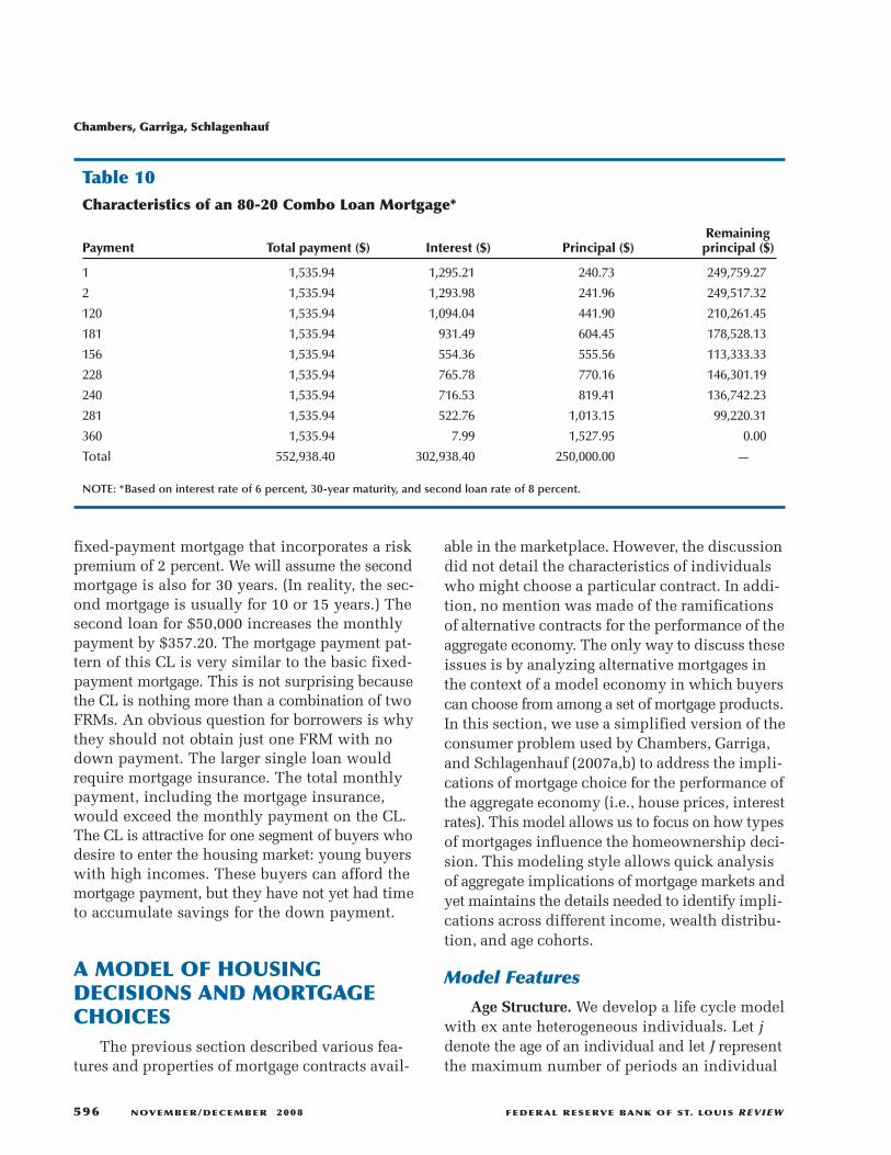
fixed-payment mortgage that incorporates a riskpremium of 2 percent. We will assume the secondmortgage is also for 30 years. (In reality, the sec-ond mortgage is usually for 10 or 15 years.) Thesecond loan for $50,000 increases the monthlypayment by $357.20. The mortgage payment pat-tern of this CL is very similar to the basic fixed-payment mortgage. This is not surprising becausethe CL is nothing more than a combination of twoFRMs. An obvious question for borrowers is whythey should not obtain just one FRM with nodown payment. The larger single loan wouldrequire mortgage insurance. The total monthlypayment, including the mortgage insurance,would exceed the monthly payment on the CL.The CL is attractive for one segment of buyers whodesire to enter the housing market: young buyerswith high incomes. These buyers can afford themortgage payment, but they have not yet had timeto accumulate savings for the down payment.

A MODEL OF HOUSINGDECISIONS AND MORTGAGECHOICES

The previous section described various fea-tures and properties of mortgage contracts avail-

able in the marketplace. However, the discussiondid not detail the characteristics of individualswho might choose a particular contract. In addi-tion, no mention was made of the ramificationsof alternative contracts for the performance of theaggregate economy. The only way to discuss theseissues is by analyzing alternative mortgages inthe context of a model economy in which buyerscan choose from among a set of mortgage products.In this section, we use a simplified version of theconsumer problem used by Chambers, Garriga,and Schlagenhauf (2007a,b) to address the impli-cations of mortgage choice for the performance ofthe aggregate economy (i.e., house prices, interestrates). This model allows us to focus on how typesof mortgages influence the homeownership deci-sion. This modeling style allows quick analysisof aggregate implications of mortgage markets andyet maintains the details needed to identify impli-cations across different income, wealth distribu-tion, and age cohorts.

Model Features

Age Structure. We develop a life cycle modelwith ex ante heterogeneous individuals. Let jdenote the age of an individual and let J representthe maximum number of periods an individual



Table 10Characteristics of an 80-20 Combo Loan Mortgage*


1 1,535.94 1,295.21 240.73 249,759.27

2 1,535.94 1,293.98 241.96 249,517.32

120 1,535.94 1,094.04 441.90 210,261.45

181 1,535.94 931.49 604.45 178,528.13

156 1,535.94 554.36 555.56 113,333.33

228 1,535.94 765.78 770.16 146,301.19

240 1,535.94 716.53 819.41 136,742.23

281 1,535.94 522.76 1,013.15 99,220.31

360 1,535.94 7.99 1,527.95 0.00

Total 552,938.40 302,938.40 250,000.00 —

NOTE: *Based on interest rate of 6 percent, 30-year maturity, and second loan rate of 8 percent.

can live. At every period, an individual facesmortality risk and uninsurable labor-earninguncertainty. The survival probability, conditionalon the individual being alive at age j, is denotedby ψj+1 � [0,1], with ψ1 = 1 and ψj+1 = 0. Earninguncertainty implies that the individual is subjectto income shocks that cannot be insured via pri-vate contracts. In addition, we assume that annu-ity markets for mortality risk are absent. The lackof these insurance markets creates a demand forprecautionary savings to minimize fluctuations inconsumption goods, c, and in the consumptionof housing services, s, over the life cycle.

Preferences. Individual preferences rankgoods (consumption and housing) according toa utility function, u�c,s�. The utility functionhas the property that additional consumptionincreases utility and also results in decliningmarginal utility. Consumption over periods isdiscounted at rate β and, thus, lifetime utility isdefined as

The assumption that utility is separable overtime allows for a simple recursive structure ofpreferences for every realization of uncertainty:

Using the definition of expected lifetime utility,we can write the previous expression as

where

represents the future lifetime expected utility.Asset Structure. Individuals have access to

a portfolio of assets to mitigate income andmortality risk. We consider two distinct assets:a riskless financial asset denoted by a′ with anet return r and a risky housing durable gooddenoted by h′ with a market price, p, where theprime is used to denote future variables. To keepthings simple, we assume that the price of hous-ing does not change over time, so p = p′. This

v E u c sj

J

jj

j j11

1= ( )=

−∑ψ β , .

v u c s E u c sj

Jj

jj j1 1 1 2

2= ( ) + ( )=−∑, .β ψ β ,

v u c s Ev1 1 1 2= ( ) +, ,β

v u c sj

Jj

jj j2 2

2= ( )=−∑ ψ β ,

assumption simplifies the problem becausehouseholds do not need to anticipate changes inhouse prices. A housing investment of size h′ canbe thought of as the number of square feet in thehouse. A house of size h′ yields s services.8 If ahousehold does not invest in housing, h = 0, thehousehold is a renter and must purchase housingservices from a rental market. The rental priceof a unit of housing services is R.

Housing investment is financed through long-term mortgage contracts and is subject to transac-tion costs. We need to summarize the informationrequired so that the monthly payment, remainingprincipal, and equity position in the house can beidentified for any mortgage contract. This criticalinformation consists of the house size, h, the typeof mortgage contract, z, and the remaining lengthof the mortgage, n. This information set can beused to identify the desired information concern-ing a household’s mortgage contract.

Household Income. Household incomevaries over the buyer’s life cycle and depends onwhether the individual is a worker or a retiree.For workers younger than the mandatory retire-ment age, j < j*, income is stochastic and dependson the basic wage income, w, a life cycle termthat depends on age, υj, and the persistent idio-syncratic component, ε, drawn from a probabilitydistribution that evolves according to the transi-tion law, Πε,ε ′. For an individual older than j*, aretirement benefit, θ, is received from the govern-ment equal to θ. Income can be specified as

In the presence of mortality risk and missing annu-ity markets, we assume borrowing constraints,a′ ≥ 0, to prevent individuals (buyers and renters)from dying with negative wealth. We also assumethat households are born with initial wealthdependent on their initial income level.

The Decision Problem. Individuals makedecisions about consumption goods, c, housingservices, s, a mortgage contract type, z, and

y a jw r a j j

r aj

j, , ,

, if ,

, if Äε υ

ευ

θ( ) =

+ +( ) <

+ +( )

∗1

1 jj j≥

∗.



8 For the sake of simplicity, we assume a linear relationship betweenhouse size and services generated. In other words, s = h′.

investment in assets, a′, and housing, h′. Theindividual’s current-period budget constraintdepends on the household’s asset holdings, thecurrent housing investment, the remaining lengthof the mortgage, labor income shock, and age.We can isolate five possible decision problemsthat a household must solve.

The household value function, v, is describedby a vector of so-called state variables that providesufficient information of the position of the indi-vidual at the start of the period. The state vectoris characterized by the level of assets at the startof the period, a, the prior-period housing position,h, the number of periods remaining on an existingmortgage, n, the mortgage contract type, z, thevalue of the current-period idiosyncratic shock,ε, and the age of the individual, j. To shortennotation of the individual’s characteristics, wedefine x = �a,h,n,z,ε,j�. Using a recursive approach,we know that the household decisions forc,s,z,a′ and h′ depend on the x vector. For exam-ple, suppose that x contains the following infor-mation, x = �1000,2000,56,FRM,2,36�. This vectortells us that the individual has $1,000 of non-housing wealth, a 2,000-square-foot home with amarket value given by p × 2,000, where p repre-sents the given price per square foot, 56 pendingmortgage payments with the bank, an FRM, theincome shock this period is two times averageincome, and the individual’s age is 36. The deci-sions made by this individual will differ fromthose of an individual who has a different statevector x = �20000,2000,56,FRM,2,41�, becausethe second individual has more wealth and is 5years older. For individuals who do not own ahome, the information vector would have manyzero entries, such as x = �a,0,0,0,ε,j �.

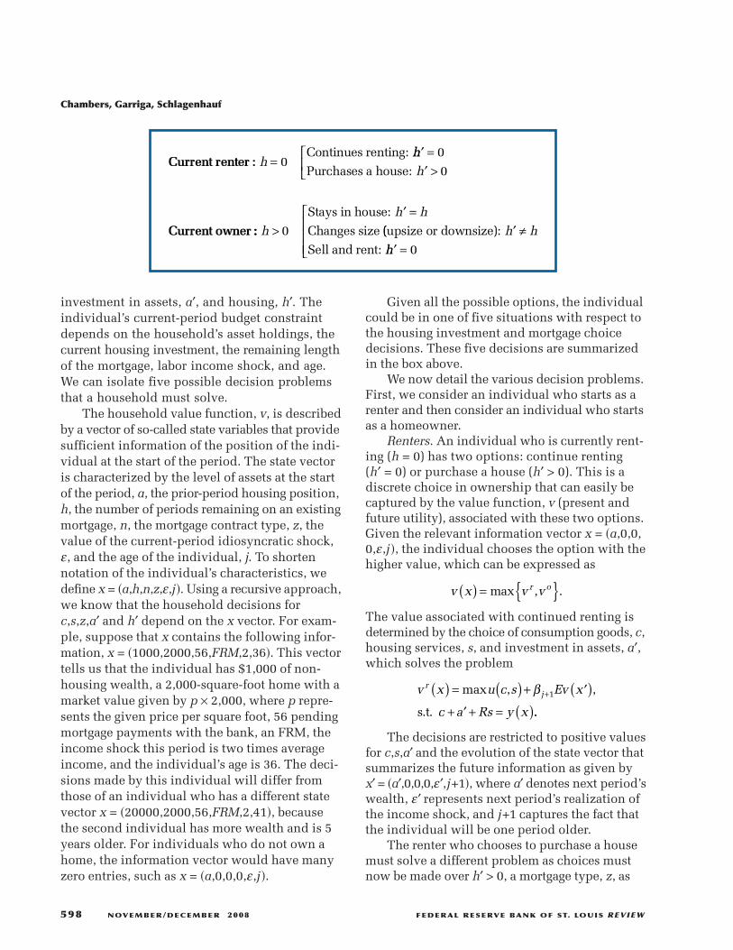
Given all the possible options, the individualcould be in one of five situations with respect tothe housing investment and mortgage choicedecisions. These five decisions are summarizedin the box above.

We now detail the various decision problems.First, we consider an individual who starts as arenter and then consider an individual who startsas a homeowner.

Renters. An individual who is currently rent-ing (h = 0) has two options: continue renting (h′ = 0) or purchase a house (h′ > 0). This is adiscrete choice in ownership that can easily becaptured by the value function, v (present andfuture utility), associated with these two options.Given the relevant information vector x = �a,0,0,0,ε,j �, the individual chooses the option with thehigher value, which can be expressed as

The value associated with continued renting isdetermined by the choice of consumption goods, c,housing services, s, and investment in assets, a′,which solves the problem

The decisions are restricted to positive valuesfor c,s,a′ and the evolution of the state vector thatsummarizes the future information as given by x′ = �a′,0,0,0,ε ′,j+1�, where a′ denotes next period’swealth, ε ′ represents next period’s realization ofthe income shock, and j+1 captures the fact thatthe individual will be one period older.

The renter who chooses to purchase a housemust solve a different problem as choices mustnow be made over h′ > 0, a mortgage type, z, as

v x v vr o( ) = { }max , .

v x u c s Ev x

c a Rs y x

rj( ) = ( ) + ′( )

+ ′ + = ( )+max , ,

s.t.

β 1

..



CCuurrrreenntt� � rreenntteerr ::� � � � ��

h =′

0Continues� renting: hh

h=′ >

0

0Purchases� a� house:�

CCuurrrreenntt� � oowwnneerr ::::� � � � ��

hh h

>′ =

0

Stays� in� house:

Changes� size� ((upsize� or� downsize):

Sell� and� rent:

��

′ ≠′

h hhh =

0

well as c, s, and a′. This decision problem can bewritten as

It should be noted that a purchase of a houserequires two up-front expenditures: transactioncosts (i.e., realtors’ fees, closing costs) that areproportional to the value of the house, ϕbph′, anda down payment to the mortgage bank for a frac-tion of the value of the house, χ�z′ � (i.e., 20 per-cent of the purchase price). These payments areincurred only at the time of the purchase. Home -owners also must make mortgage payments. Thesepayments are denoted by m�x� and depend on rele-vant variables, such as the loan amount, �1 – χ�ph′,the type of mortgage (i.e., FRM vs. ARM), thelength of the contract (i.e., 30 or 15 years), and theinterest rate associated with the loan. It is impor-tant to restate that a homeowner who purchasesa house of size h′ receives s units of housing con-sumption. The value of these housing services isdenoted by Rsh. This value does not appear in thebudget constraint because these services are con-sumed internally. As a result, the value of servicesgenerated is canceled by the value of servicesconsumed internally. The household’s decisionsinfluence the information state in the followingperiod; that is, x′ = �a′,h′,N�z� – 1,z′,ε ′,j+1�. Again,to determine whether an individual continues torent or purchases a home, we need to solve bothproblems—vr�x� and v0�x�— and find the onethat yields the highest value. When vr�x� > v 0�x�,the individual continues to rent; otherwise he orshe will become a homeowner.

Owners. The decision problem for an individ-ual who currently owns a house, (h > 0), has asimilar structure. However, a homeowner faces adifferent set of options: stay in the same house,(h′ = h), purchase a different house, (h′ ≠ h), or sellthe house and acquire housing services throughthe rental market, (h′ = 0). Given the relevantinformation x = �a,h,n,z,ε,j�, the individual solves

Each of these three different values is calculatedby solving three different decision problems. If the

v x u c s Ev x

c a z

oj

b

( ) = ( ) + ′( )+ ′ + + ′(

+max , ,

s.t.

β

ϕ χ1

)) ′ + ( ) = ( )ph m x y x .

v x v v vs c r( ) = { }max , , .

homeowner decides to stay in the current house,the optimization problem can be written as

This problem is very simple, because the home-owner must make decisions only on consumptionand saving after making the mortgage payment.If the schedule of pending mortgage paymentsshows zero, n = 0, then the implied mortgagepayment is also set to zero, m�x� = 0. The futurestate of information for this case is given by x′ = �a′,h′,n′, z′,ε′,j+1�, where n′ = max{n – 1,0}.

For the homeowner who decides to eitherupsize or downsize, (h ≠ h′), the problem becomes

This individual must sell the existing propertyto purchase a new one. The choices depend onthe income received from selling the property, ph,net of transactions costs from selling, ϕs, and theremaining principal, D�n,z�, owed to the lender.The standing balance depends on whether themortgage has been paid off (n = 0 and D�n,z� = 0)or not (n > 0 and D�n,z� > 0) and the type of loancontract. For example, mortgage loans with a slowamortization usually imply large remaining prin-cipal when the property is sold over the lengthof the loan, whereas contracts such as the con-stant amortization imply a much faster repay-ment. A new loan, z′, must be acquired if theindividual upsizes and purchases a new house,h′ > 0. The relevant future information is givenby x′ = �a′,h′,N – 1, z′,ε′,j+1�.

Finally, we solve the problem of a homeownerwho sells the house, h > 0, and becomes a renter,h′ = 0.9 The optimization problem is very similarto the previous one. However, in this case the indi-vidual must sell the home and rent, Rs. Formally,

v x u c h Ev x

c a z

cj

b

( ) = ′( ) + ′( )+ ′ + + ′(

+max ,

s.t.

β

ϕ χ1

)) ′ + ( )= ( ) + −( ) − ( )

ph m x

y x ph D n zs1 ϕ , .

v x u c h Ev x

c a y x m x

sj( ) = ′( ) + ′( )

+ ′ = ( ) −+max ,

s.t.

β 1

(( ).



9 In the last period, all households must sell h, rent housing services,and consume all their assets, a, as a bequest motive which is notin the model. In the last period, h′ = a′ = 0.

where the relevant future information is simplygiven by x′= �a′,0,0,0,ε′,j+1�.

Given the initial information summarized inx, the choice of whether to stay in the house,change the housing size, or sell the house andbecome a renter depends on the values of vs, vc,and vr.

Aggregation and Parameterization

We want our model economy to be consistentwith certain features of the U.S. economy. In par-ticular, we want to ensure that the choices of func-tional forms and parameter values are consistentwith key features of the U.S. housing market.Replicating these features requires aggregatingthe microeconomic behavior of all the householdsin the economy. Because individuals are hetero-geneous along six different dimensions—level ofwealth, housing holdings, pending mortgage pay-ments, type of mortgage used to finance the house,income shock, and age—our aggregation needsto take into account the number of individualswho have the same characteristics and the sumacross these characteristics. To aggregate thesedimensions, we define Φ�x� as the fraction of indi-viduals who have a given level of characteristicsx = �a,h,n,z,ε,j�.

We can calculate aggregate statistics of theeconomy by taking the weighted average of all thehousehold-level decisions across characteristics.As an example we would generate the aggregatehousing stock, wealth, and consumption of hous-ing services (or square feet) by calculating

The model can generate other aggregates ofinterest in a similar manner. We start by discussinghow the model is parameterized.

Demographics. A period in the model is takento be three years. Individuals enter the laborforce at age 20 (model period 1) and potentially

v x u c s Ev x

c a Rs y x

rj( ) = ( ) + ′( )

+ ′ + = ( )+max , ,

s.t.

β 1

++ −( ) − ( ) 1 ϕs ph D n z, ,

H h x dx

W a x dx

S s x dx

= ∫ ′( ) ( )= ∫ ′( ) ( )= ∫ ( ) ( )

Φ

Φ

Φ

;

;

.

live until age 86 (model period 23). Retire ment isassumed to be mandatory at age 65 (model period16). Individuals survive to the next period withprobability ψj+1.10 The size of the age-specificcohorts, µj, needs to be specified. Because of ourfocus on steady-state equilibrium, these sharesmust be consistent with the stationary populationdistribution. As a result, these shares are deter-mined from µj = ψjµj–1/�1 + ρ� for j = 1,2,…,J and

where ρ denotes the population growth rate.Using the resident population as the measure ofthe population, the annual growth rate is set at1.2 percent.

Functional Forms. The choice of preferencesis based on empirical evidence. The first-ordercondition that determines the optimal amountof housing consumption is denoted by

where at the optimum sj = h′j. Jeske (2005) docu-ments that the hj/cj ratio is increasing by age j. Hepoints out that standard homothetic preferencesover consumption and housing services,

imply a constant ratio

because the parameters γ and σ and the rentalprice R do not vary across age. Therefore, thispreference specification is inconsistent with theempirical evidence over the life cycle. A prefer-ence structure consistent with the evidence isdenoted by

where the implied first-order condition isdenoted by

jJ

j=∑ =1 1µ ,

u

uR

s

c

j

j

= ,

u c s c sj j j j, ,( ) = + −( ) γ γσ σ σ11

h

c Rj

j

=−( )

−11

1γγ

σ

,

u c sc s

, ,( ) =−

+ −( )−

− −

γσ

γσ

σ σ1

1

1

2

1 2

11

1



10 These probabilities are set at survival rates observed in 1994, andthe data are from the National Center for Health Statistics (U.S.Department of Health and Human Services, 1994).

This expression represents a nonlinear rela-tionship between hj and cj that varies by age, j.The coefficients, σ1 and σ2, determine the curva-ture of the utility function with respect to con-sumption and housing services. The relative ratioof σ1 and σ2 determines the growth rate of thehousing-to-consumption ratio. A larger curvaturein consumption relative to the curvature in hous-ing services implies that the marginal utility ofconsumption exhibits relatively faster diminish-ing returns. When household income increasesover the life cycle (or different idiosyncratic laborincome shocks), a larger fraction of resources isallocated to housing services. We set σ2 = 1 andσ2 = 3 to match the observed average growth ratewhile the preference parameter γ is estimated.The discount factor, β, is set at 0.976, which isderived from Chambers, Garriga, and Schlagenhauf(2007a).

Endowments. Workers are assumed to havean inelastic labor supply, but the effective qual-ity of their supplied labor depends on two com-ponents. One component is age specific, υj, andis designed to capture the hump in life cycleearnings. We use U.S. Census Bureau (1994) datato construct this variable. The other componentcaptures the stochastic component of earningsand is based on Storesletten, Telmer, and Yaron(2004). We discretize this income process into afive-state Markov chain using the methodologypresented by Tauchen (1986). Our reported valuesreflect the three-year horizon used in the model.As a result, the efficiency values associatedwith each possible productivity value, ε, are

and the transition matrix is

h

c Rj

j

σ

σγ

γ

2

1

1=

−( ).

ε ∈ = { }E 4 41 3 51 2 88 2 37 1 89. . . . ., , , , ,

π =

0 47 0 33 0 14 0 05 0 01

0 29 0 33 0 23 0 11 0 03

0

. . . . .

. . . . .

.. . . . .

. . . . .

.

12 0 23 0 29 0 24 0 12

0 03 0 11 0 23 0 33 0 29

0 011 0 05 0 14 0 33 0 47. . . .

.

Each household is born with an initial assetposition. This assumption accounts for the factthat some of the youngest buyers who purchasehousing have some wealth. Failure to allow forthis initial asset distribution creates a bias againstthe purchase of homes in the earliest age cohorts.As a result, we use the asset distribution observedin Panel Study on Income Dynamics (Institute forSocial Research, 1994) to match the initial distri-bution of wealth for the cohort of age 20 to 23.Each income state has assigned the correspondinglevel of assets to match the nonhousing wealth-to-earnings ratio. We choose the basic level ofearnings, w, as a scaler to match labor earningsover total earnings.

Housing. The housing market introduces anumber of parameters. The purchase of a houserequires a mortgage and down payment. In thispaper, we focus on the 30-year FRM as the bench-mark mortgage. As a result of the assumptionthat a period is three years, we set the mortgagelength, N, to 10 periods. The down payment, χ,is set to 20 percent (matching facts from the 2004U.S. Department of Commerce American HousingSurvey, AHS). Buying and selling property issubject to transaction costs. We assume that allthese costs are paid by the buyer and set σs = 0and σb = 0.06.

Because of the lumpy nature of the housinginvestment (i.e., movement from H = 0 to H > 0),the specification of the second point in the hous-ing grid has important ramifications. This gridpoint, h, determines the minimum house size andhas implications for the timing of investments inhousing, wealth portfolio decisions, and thehomeownership rate. We determine the size ofthis grid point as part of the estimation problemto avoid inadvertent implications on the resultscaused by this variable.

Estimation

We estimate five parameters using an exactlyidentified method of moments approach. Theparameters that need to be estimated are theinterest rate, r, the rental rate for housing, R, theprice of housing, p, the wage rate w, and the sizeof the smallest housing investment position, h.We identify these parameter values so that the



resulting aggregate statistics in the model econ-omy are equal to five targets observed in the U.S.economy.

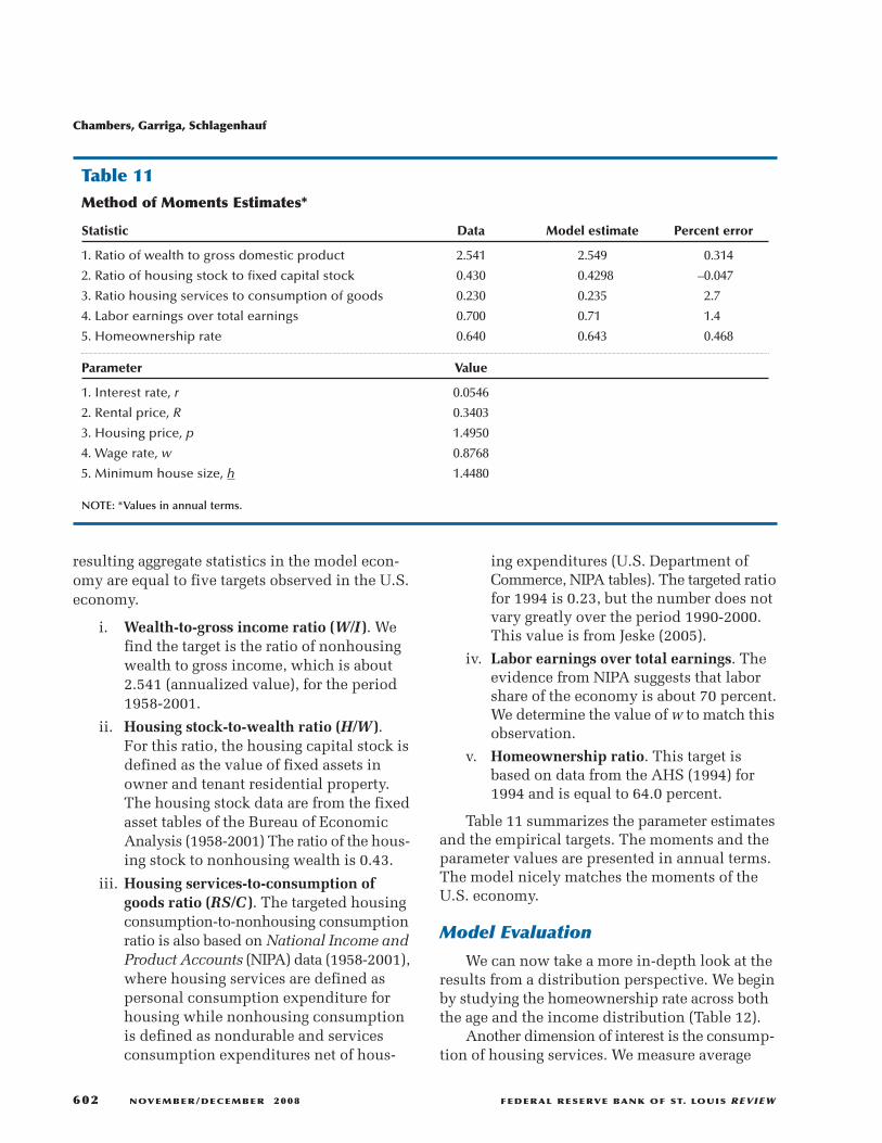
i. Wealth-to-gross income ratio (W/I ). Wefind the target is the ratio of nonhousingwealth to gross income, which is about2.541 (annualized value), for the period1958-2001.

ii. Housing stock-to-wealth ratio (H/W ). For this ratio, the housing capital stock isdefined as the value of fixed assets inowner and tenant residential property.The housing stock data are from the fixedasset tables of the Bureau of EconomicAnalysis (1958-2001) The ratio of the hous-ing stock to nonhousing wealth is 0.43.

iii. Housing services-to-consumption ofgoods ratio (RS/C ). The targeted housingconsumption-to-nonhousing consumptionratio is also based on National Income andProduct Accounts (NIPA) data (1958-2001),where housing services are defined aspersonal consumption expenditure forhousing while nonhousing consumptionis defined as nondurable and servicesconsumption expenditures net of hous-

ing expenditures (U.S. Department ofCommerce, NIPA tables). The targeted ratiofor 1994 is 0.23, but the number does notvary greatly over the period 1990-2000.This value is from Jeske (2005).

iv. Labor earnings over total earnings. Theevidence from NIPA suggests that laborshare of the economy is about 70 percent.We determine the value of w to match thisobservation.

v. Homeownership ratio. This target isbased on data from the AHS (1994) for1994 and is equal to 64.0 percent.

Table 11 summarizes the parameter estimatesand the empirical targets. The moments and theparameter values are presented in annual terms.The model nicely matches the moments of theU.S. economy.

Model Evaluation

We can now take a more in-depth look at theresults from a distribution perspective. We beginby studying the homeownership rate across boththe age and the income distribution (Table 12).

Another dimension of interest is the consump-tion of housing services. We measure average



Table 11Method of Moments Estimates*

Statistic Data Model estimate Percent error

1. Ratio of wealth to gross domestic product 2.541 2.549 0.314

2. Ratio of housing stock to fixed capital stock 0.430 0.4298 –0.047

3. Ratio housing services to consumption of goods 0.230 0.235 2.7

4. Labor earnings over total earnings 0.700 0.71 1.4

5. Homeownership rate 0.640 0.643 0.468

Parameter Value

1. Interest rate, r 0.0546

2. Rental price, R 0.3403

3. Housing price, p 1.4950

4. Wage rate, w 0.8768

5. Minimum house size, h 1.4480

NOTE: *Values in annual terms.

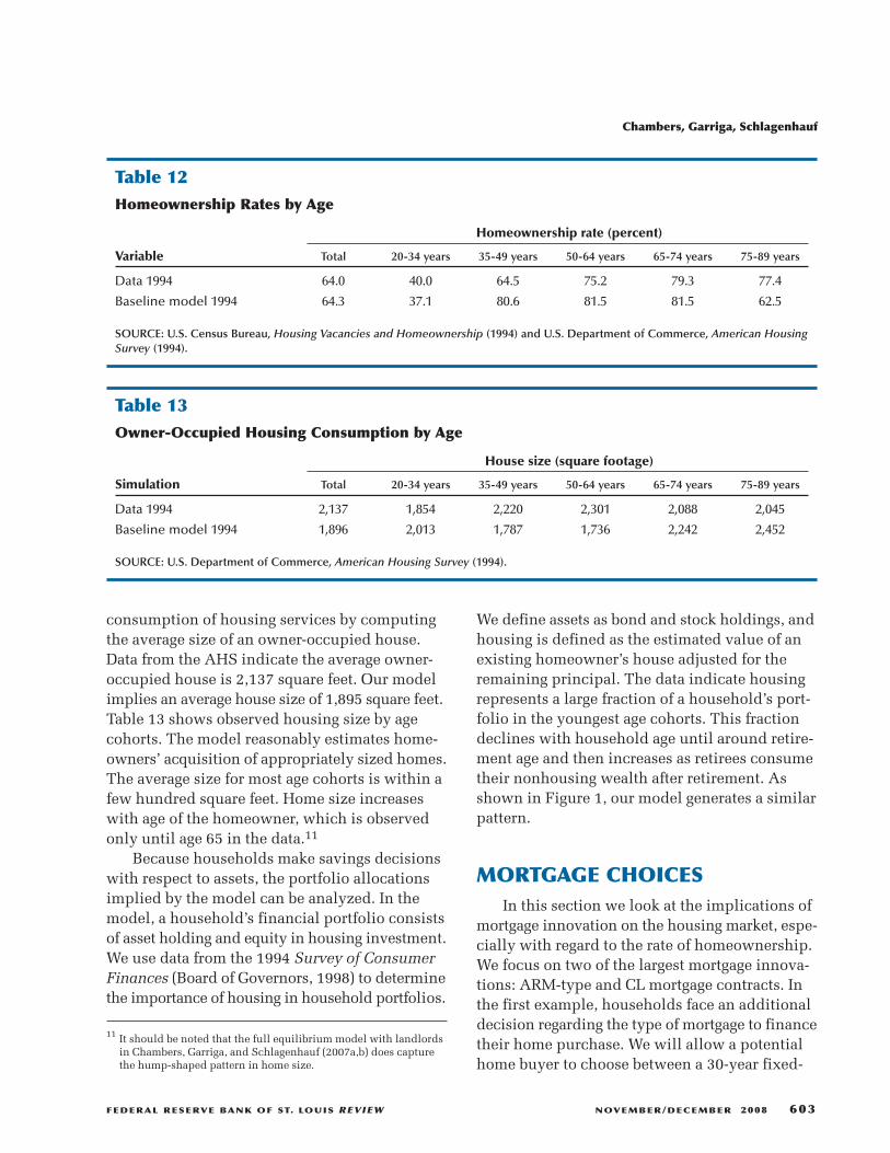
consumption of housing services by computingthe average size of an owner-occupied house.Data from the AHS indicate the average owner-occupied house is 2,137 square feet. Our modelimplies an average house size of 1,895 square feet.Table 13 shows observed housing size by agecohorts. The model reasonably estimates home-owners’ acquisition of appropriately sized homes.The average size for most age cohorts is within afew hundred square feet. Home size increaseswith age of the homeowner, which is observedonly until age 65 in the data.11

Because households make savings decisionswith respect to assets, the portfolio allocationsimplied by the model can be analyzed. In themodel, a household’s financial portfolio consistsof asset holding and equity in housing investment.We use data from the 1994 Survey of ConsumerFinances (Board of Governors, 1998) to determinethe importance of housing in household portfolios.

We define assets as bond and stock holdings, andhousing is defined as the estimated value of anexisting homeowner’s house adjusted for theremaining principal. The data indicate housingrepresents a large fraction of a household’s port-folio in the youngest age cohorts. This fractiondeclines with household age until around retire-ment age and then increases as retirees consumetheir nonhousing wealth after retirement. Asshown in Figure 1, our model generates a similarpattern.

MORTGAGE CHOICESIn this section we look at the implications of

mortgage innovation on the housing market, espe-cially with regard to the rate of homeownership.We focus on two of the largest mortgage innova-tions: ARM-type and CL mortgage contracts. Inthe first example, households face an additionaldecision regarding the type of mortgage to financetheir home purchase. We will allow a potentialhome buyer to choose between a 30-year fixed-



11 It should be noted that the full equilibrium model with landlordsin Chambers, Garriga, and Schlagenhauf (2007a,b) does capturethe hump-shaped pattern in home size.

Table 12Homeownership Rates by Age

Homeownership rate (percent)

Variable Total 20-34 years 35-49 years 50-64 years 65-74 years 75-89 years

Data 1994 64.0 40.0 64.5 75.2 79.3 77.4

Baseline model 1994 64.3 37.1 80.6 81.5 81.5 62.5

SOURCE: U.S. Census Bureau, Housing Vacancies and Homeownership (1994) and U.S. Department of Commerce, American HousingSurvey (1994).

Table 13Owner-Occupied Housing Consumption by Age

House size (square footage)

Simulation Total 20-34 years 35-49 years 50-64 years 65-74 years 75-89 years

Data 1994 2,137 1,854 2,220 2,301 2,088 2,045

Baseline model 1994 1,896 2,013 1,787 1,736 2,242 2,452

SOURCE: U.S. Department of Commerce, American Housing Survey (1994).

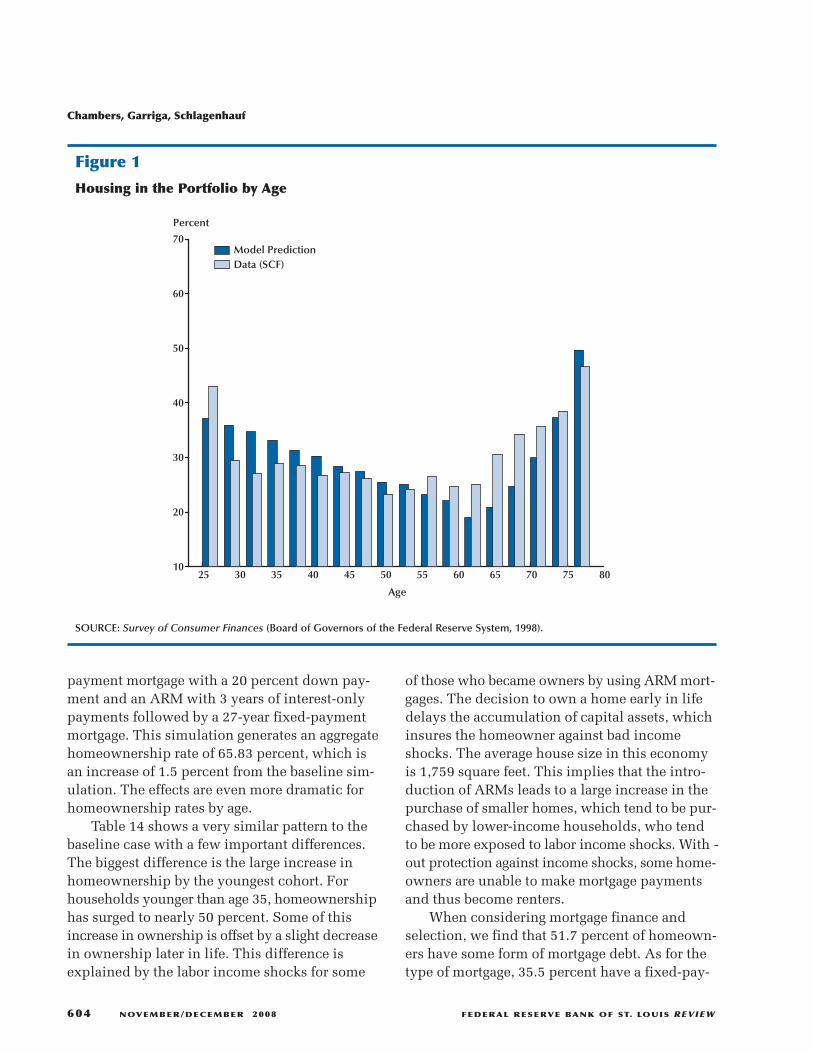
payment mortgage with a 20 percent down pay-ment and an ARM with 3 years of interest-onlypayments followed by a 27-year fixed-paymentmortgage. This simulation generates an aggregatehomeownership rate of 65.83 percent, which isan increase of 1.5 percent from the baseline sim-ulation. The effects are even more dramatic forhomeownership rates by age.

Table 14 shows a very similar pattern to thebaseline case with a few important differences.The biggest difference is the large increase inhomeownership by the youngest cohort. Forhouseholds younger than age 35, homeownershiphas surged to nearly 50 percent. Some of thisincrease in ownership is offset by a slight decreasein ownership later in life. This difference isexplained by the labor income shocks for some

of those who became owners by using ARM mort-gages. The decision to own a home early in lifedelays the accumulation of capital assets, whichinsures the homeowner against bad incomeshocks. The average house size in this economyis 1,759 square feet. This implies that the intro-duction of ARMs leads to a large increase in thepurchase of smaller homes, which tend to be pur-chased by lower-income households, who tendto be more exposed to labor income shocks. With -out protection against income shocks, some home-owners are unable to make mortgage paymentsand thus become renters.

When considering mortgage finance andselection, we find that 51.7 percent of homeown-ers have some form of mortgage debt. As for thetype of mortgage, 35.5 percent have a fixed-pay-



25 30 35 40 45 50 55 60 65 70 75 8010

20

30

40

50

60

70

Age

Percent

Model PredictionData (SCF)

Figure 1

Housing in the Portfolio by Age

SOURCE: Survey of Consumer Finances (Board of Governors of the Federal Reserve System, 1998).

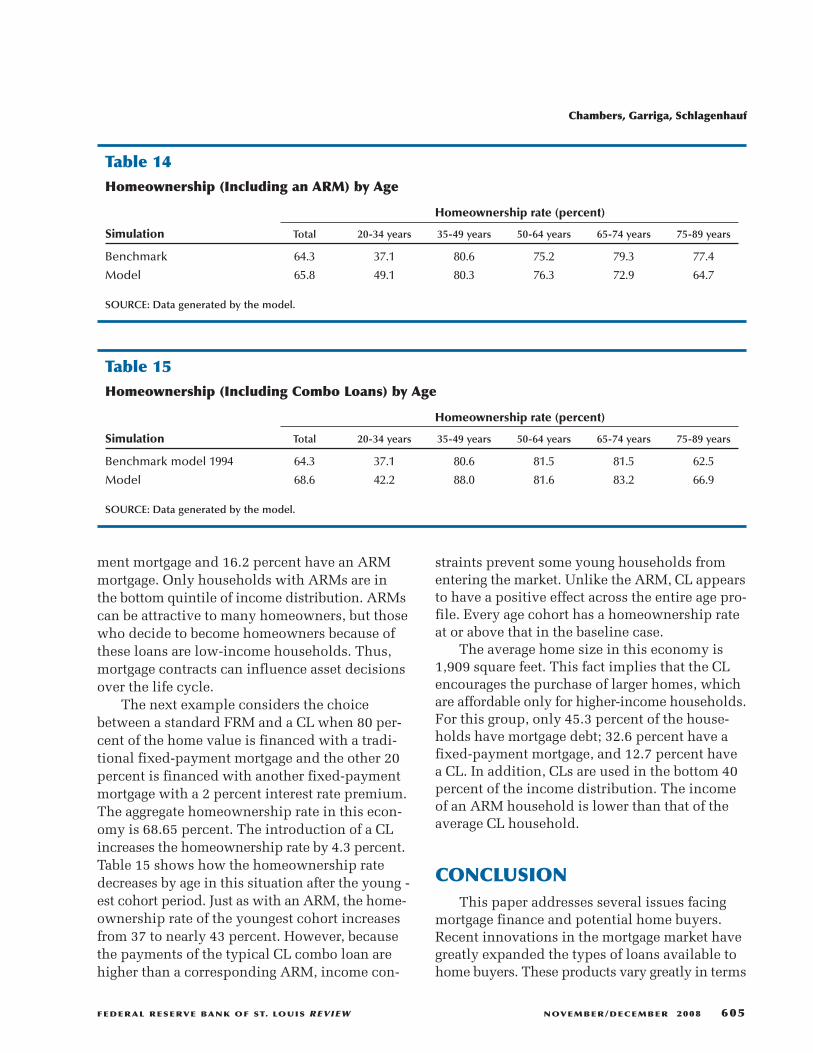
ment mortgage and 16.2 percent have an ARMmortgage. Only households with ARMs are inthe bottom quintile of income distribution. ARMscan be attractive to many homeowners, but thosewho decide to become homeowners because ofthese loans are low-income households. Thus,mortgage contracts can influence asset decisionsover the life cycle.

The next example considers the choicebetween a standard FRM and a CL when 80 per-cent of the home value is financed with a tradi-tional fixed-payment mortgage and the other 20percent is financed with another fixed-paymentmortgage with a 2 percent interest rate premium.The aggregate homeownership rate in this econ-omy is 68.65 percent. The introduction of a CLincreases the homeownership rate by 4.3 percent.Table 15 shows how the homeownership ratedecreases by age in this situation after the young -est cohort period. Just as with an ARM, the home-ownership rate of the youngest cohort increasesfrom 37 to nearly 43 percent. However, becausethe payments of the typical CL combo loan arehigher than a corresponding ARM, income con-

straints prevent some young households fromentering the market. Unlike the ARM, CL appearsto have a positive effect across the entire age pro-file. Every age cohort has a homeownership rateat or above that in the baseline case.

The average home size in this economy is1,909 square feet. This fact implies that the CLencourages the purchase of larger homes, whichare affordable only for higher-income households.For this group, only 45.3 percent of the house-holds have mortgage debt; 32.6 percent have afixed-payment mortgage, and 12.7 percent havea CL. In addition, CLs are used in the bottom 40percent of the income distribution. The incomeof an ARM household is lower than that of theaverage CL household.

CONCLUSIONThis paper addresses several issues facing

mortgage finance and potential home buyers.Recent innovations in the mortgage market havegreatly expanded the types of loans available tohome buyers. These products vary greatly in terms



Table 14Homeownership (Including an ARM) by Age



Benchmark 64.3 37.1 80.6 75.2 79.3 77.4

Model 65.8 49.1 80.3 76.3 72.9 64.7

SOURCE: Data generated by the model.

Table 15Homeownership (Including Combo Loans) by Age



Benchmark model 1994 64.3 37.1 80.6 81.5 81.5 62.5

Model 68.6 42.2 88.0 81.6 83.2 66.9

SOURCE: Data generated by the model.

of payment size, composition of interest versusprincipal, and amortization schedule. Some prod-ucts, such as interest-only loans, increase afford-ability by reducing payment size. However, theseproducts typically slow accumulation of equityand thus become less attractive for wealth accu-mulation. Some mortgage types can generatenegative amortization, which would seem highlyunattractive to potential mortgage lenders. Otherproducts, such as CLs, seek to increase afford-ability by reducing down payment requirements.These mortgages are characterized by larger mort-gage payments. Given the typical governmentstance of seeking greater homeownership, bothtypes of products appear successful in this regard.

In a standard macroeconomic model, we findthat the typical ARM should generate largeincreases in the homeownership rate of younghouseholds. However, because of a delay in cap-ital asset accumulation, lower homeownershipmay be found for older households. CLs also tendto drive up homeownership. For young house-holds this increase in homeownership is not aspronounced as with ARMs, but with no apparentreduction in homeownership later in the life cycle.Thus, it should come as no surprise that the intro-duction of these mortgage products coincidedwith the observed increase in homeownershipfrom 1995 through 2005. It should also not besurprising that the homeownership rate declinesas these instruments are removed from the mort-gage market.

REFERENCESChambers, Matthew; Garriga, Carlos andSchlagenhauf, Don. “Accounting for Changes inthe Homeownership Rate.” International EconomicReview, July 2007a (forthcoming).

Chambers, Matthew; Garriga, Carlos andSchlagenhauf, Don. “The Tax Treatment ofHomeowners and Landlords,” Working Paper,Florida State University, July 2007b.

Board of Governors of the Federal Reserve System.Survey of Consumer Finances, 1998; www.federalreserve.gov/pubs/oss/oss2/scfindex.html.

Institute for Social Research. Panel Study of IncomeDynamics, 1994. Ann Arbor, MI: Institute forSocial Research, University of Michigan;http://psidonline.irs.umich.edu/search.

Jeske, Karsten. “Macroeconomic Models withHeterogenous Agents and Housing.” FederalReserve Bank of Atlanta Economic Review, FourthQuarter 2005, 90(4), pp. 39-56; www.frbatlanta.org/filelegacydocs/erq405_jeske.pdf.

McDonald, Daniel J. and Thornton, Daniel L. “A Primer on the Mortgage Market and MortgageFinance.” Federal Reserve Bank of St. LouisReview, January/February 2008, 90(1), pp. 31-45;http://research.stlouisfed.org/publications/review/08/01/McDonald.pdf.

Storesletten, Kjetil, C.; Telmer, Chris I. and Yaron,Amir. “Consumption and Risk Sharing over theLife Cycle.” Journal of Monetary Economics, April2004, 51(3), pp. 609-33.

The Mortgage Market Statistical Annual. Bethesda,MD: Inside Mortgage Finance Publications, 2007.

Tauchen, George. “Finite State Markov-ChainApproximation to Univariate and VectorAutoregressions.” Economic Letters, 1986, 20(2),pp. 177-81.

U.S. Bureau of Economic Analysis. National Incomeand Product Accounts; www.bea.gov/national.

U.S. Census Bureau. Housing Vacancies andHomeownership; www.census.gov/hhes/www/housing/hvs/hvs.html.

U.S. Census Bureau. Residential Finance Survey:2001—Census 2000 Special Reports (reportCENSR-27); www.census.gov/prod/2005pubs/census-27.pdf.

U.S. Census Bureau, U.S. Department of Commerce,Economics and Statistics Administration. CurrentPopulation Reports, Money Income of Households,Families, and Persons in the United States: 1994(Series P60); www.census.gov/prod/www/abs/income.html.



http://www.federalreserve.gov/pubs/oss/oss2/scfindex.html

http://www.frbatlanta.org/filelegacydocs/erq405_jeske.pdf

http://www.frbatlanta.org/filelegacydocs/erq405_jeske.pdf

U. S. Department of Commerce, Bureau of theCensus. American Housing Survey, 2004 NationalFile; www.census.gov/hhes/www/housing/ahs/metropolitandata.html.

U.S. Department of Commerce, Bureau of EconomicAnalysis. National Income and Product Accounts;www.bea.gov/bea/dn/nipaweb/index.asp.

U.S. Department of Health and Human Services,Centers for Disease Control and Prevention, NationalCenter for Health Statistics, Vital Statistics of theUnited States, 1994, Vol II, Mortality, Part A. section 6; www.cdc.gov/nchs/data/lifetables/life94_2.pdf.



APPENDIXAlm, James and J. Follain, James R., Jr. “Alternative Mortgage Instruments, the Tilt Problem and ConsumerWelfare.” Journal of Financial and Quantitative Analysis, March 1984, 19(1), pp. 113-26.

Berkovec, James and Fullerton, Don. “A General Equilibrium Model of Housing, Taxes and Portfolio Choice.”Journal of Political Economy, April 1992, 100(2), pp. 390-429.

Campbell, John Y. “Household Finance,” Journal of Finance, August 2006, 61(4), 1553-604.

Campbell, John Y. and Cocco, Joao F. “Household Risk Management and Optimal Mortgage Choice.” QuarterlyJournal of Economics, November 2003, 118(4), pp. 1449-94.

Chambers, Matthew; Garriga, Carlos and Schlagenhauf, Don. “The Loan Structure and Housing Tenure Decisionsin an Equilibrium Model of Mortgage Choice.” Working Paper 2008-024A, July 2008, Federal Reserve Bankof St. Louis; http://research.stlouisfed.org/wp/2008/2008-024.pdf, July 2008, WP 2008-024A.

Cooley, Thomas F. and Prescott, Edward C. “Economic Growth and Business Cycles” in Thomas F. Cooley, ed.,Frontiers of Business Cycle Research. Princeton, NJ: Princeton University Press, 1995, pp. 1-38.

Dhillon, Upinder S; Shilling, James D. and Simans, C.F. “Choosing Between Fixed and Adjustable RateMortgages.” Journal of Money, Credit and Banking, May 1987, 19(2), pp. 260-67.

Dunn, Kenneth B. and Spatt, Chester S. “An Analysis of Mortgage Contracting: Prepayment Penalties and theDue-on Sales Clause.” Journal of Finance, March 1985, 40(1), 293-308.

Fernández-Villaverde, Jesús and Krueger, Dirk. “Consumption and Savings over the Life-Cycle: How ImportantAre Consumer Durables?” Working Paper, University of Pennsylvania, December 19, 2005;www.econ.upenn.edu/~dkrueger/research/durables12192005sec.pdf.

Follain, James R. “Mortgage Choice.” American Real Estate and Urban Economic Associations Journal, Summer1990, 18(2), pp. 125-44.

Gouveia, Miguel and Strauss, Robert P. “Effective Federal Individual Income Tax Functions: An ExploratoryEmpirical Analysis.” National Tax Journal, June 1994, 47, pp. 317-39.

Gervais, Martin. “Housing Taxation and Capital Accumulation.” Journal of Monetary Economics, October 2002,49(7), pp. 1461-89.

Heathcoate, Jonathan and Davis, Morris. “Housing and the Business Cycle.” International Economic Review,August 2005, 46(3), pp. 751-84.

Henderson, J. Vernon and Ioannides, Yannis M. “A Model of Housing Tenure Choice.” American EconomicReview, March 1983, 73(1), pp. 98-113.

Jeske, Karsten and Krueger, Dirk. “Housing and the Macroeconomy: The Role of Implicit Guarantees forGovernment-Sponsored Enterprises.” Federal Reserve Bank of Atlanta Working Paper 2005-15, August 2005;www.frbatlanta.org/filelegacydocs/wp0515.pdf.

Kearl, James R. “Inflation, Mortgages, and Housing.” Journal of Political Economy, October 1979, 87(5, Part 1),pp. 1115-38.

LeRoy, Stephen F. “Mortgage Valuation Under Optimal Repayment.” Review of Financial Studies, Autumn 1996,9(3), pp. 817-44.

Li, Wenli. “Moving Up: Trends in Homeownership and Mortgage Indebtedness.” Federal Reserve Bank ofPhiladelphia Business Review, First Quarter 2005, pp. 26-34; www.philadelphiafed.org/files/br/brq105wl.pdf.

Li, Wenli and Yao, Rui. “The Life-Cycle Effects of House Price Changes.” Journal of Money, Credit and Banking,September 2007, 39(6), pp. 1375-409.

Nakajima, Makoto. “Rising Prices of Housing and Non-Housing Capital and Rising Earnings Instability: The Roleof Illiquidity of Housing.” Working Paper, 2003, University of Pennsylvania.

Ortalo-Magne, François and Rady, Sven. “Housing Market Dynamics: On the Contribution of Income Shocksand Credit Constraints.” Review of Economic Studies, April 2006, 73(2), pp. 459-85.

Ríos-Rull, José-Victor. “Life Cycle Economies and Aggregate Fluctuations.” Review of Economic Studies, July1996, 63(3), 465-89.

Ríos-Rull, José-Victor. “Population Changes and Capital Accumulation: The Aging of the Baby Boom.” The BEJournal of Macroeconomics, 2001, 1(1), article 7.

Ríos-Rull, José-Victor and Sanchez-Marcos, Virginia. “An Aggregate Economy with Different House Sizes.”Working Paper, September 2006, University of Pennsylvania; www.econ.umn.edu/~vr0j/papers/houaug06.pdf.

Sánchez, José Miguel. “An Estimable Dynamic Model of Housing Tenure Choice.” Unpublished manuscript,2007, Instituto de Economía, Pontificia Universidad Católica de Chile.

Stanton, Richard and Wallace, Nancy. “Mortgage Choice: What’s the Point?” Real Estate Economics, June 1998,26(2), pp. 73-205.



Mortgage Innovation, Mortgage Choice, and Housing Decisions · Mortgage Innovation, Mortgage...

Documents

Transcript of Mortgage Innovation, Mortgage Choice, and Housing Decisions · Mortgage Innovation, Mortgage...