More Branch-and-Bound Experiments in Convex Nonlinear ...More Branch-and-Bound Experiments in Convex...

Noname manuscript No.

(will be inserted by the editor)

More Branch-and-Bound Experiments in Convex

Nonlinear Integer Programming

Pierre Bonami · Jon Lee · Sven Leyffer ·

Andreas Wachter

September 29, 2011

Abstract Branch-and-Bound (B&B) is perhaps the most fundamental algorithm for

the global solution of convex Mixed-Integer Nonlinear Programming (MINLP) prob-

lems. It is well-known that carrying out branching in a non-simplistic manner can

greatly enhance the practicality of B&B in the context of Mixed-Integer Linear Pro-

gramming (MILP). No detailed study of branching has heretofore been carried out for

MINLP, In this paper, we study and identify useful sophisticated branching methods

for MINLP.

1 Introduction

Branch-and-Bound (B&B) was proposed by Land and Doig [26] as a solution method for

MILP (Mixed-Integer Linear Programming) problems, though the term was actually

coined by Little et al. [32], shortly thereafter. Early work was summarized in [27].

Dakin [14] modified the branching to how we commonly know it now and proposed its

extension to convex MINLPs (Mixed-Integer Nonlinear Programming problems); that

is, MINLP problems for which the continuous relaxation is a convex program.

Though a very useful backbone for ever-more-sophisticated algorithms (e.g., Branch-

and-Cut, Branch-and-Price, etc.), the basic B&B algorithm is very elementary. How-

Pierre BonamiLIF, Universite de Marseille, 163 Av de Luminy, 13288 Marseille, FranceE-mail: [email protected]

Jon LeeDepartment of Industrial and Operations Engineering, University of Michigan, Ann Arbor, MI48109, USAE-mail: [email protected]

Sven LeyfferArgonne National Laboratory, Argonne, IL 60439, USAE-mail: [email protected]

Andreas WachterDepartment of Industrial Engineering and Management Sciences, Northwestern University,Evanston, IL 60208, USAE-mail: [email protected]

2

ever, improving its practical robustness and performance requires several clever ideas,

a good understanding of the characteristics of the solver(s) that are employed to solve

subproblem relaxations, and a good deal of software engineering and tuning.

Two strategic decisions that can enhance the performance of B&B are the choice

of the variable to branch on at each node and the choice of the next node to process

during the tree search. Some of the key advances in choosing the branching variable

in MILP are based on the aim of fathoming nodes early in the enumeration tree. The

guiding principle for achieving this goal is to make branching decisions that result in

sharper lower bounds. “Pseudo-cost branching” for MILP was introduced by Beni-

chou et al. [8]. This technique maintains statistical estimates of the bound change in

the child nodes resulting from branching on a particular variable, by recording the

effect of previous branching decisions using that variable. “Strong branching” was in-

troduced by Applegate et al. [4] in the context of their great computational success

on the Traveling-Salesman Problem. However, it can be applied to any MILP and has

been implemented in most MILP solvers. Strong branching examines a number of can-

didate branching variables by (approximately) solving the resulting child nodes, and

chooses the “best” one as the actual branching variable. “Reliability branching,” was

proposed by Achterberg et al. [3]. It is a combination of the aforementioned pseudo-

cost and strong-branching techniques. Finally, “lookahead branching” was proposed

by Glankwamdee and Linderoth [23]. It extends strong branching by looking at grand-

children nodes.

B&B can be extended to convex MINLP in a very natural manner; i.e., the contin-

uous NLP relaxation of the original problem is solved at each node of the enumeration

tree. Gupta and Ravindran [25] conducted extensive experiments aimed at improving

the efficiency of B&B for MINLP. They assessed the branching choices from MILP

known at the time: priorities, most-fractional and pseudo-costs. The associated code

BBNLMIP [24] employed the underlying NLP (Nonlinear Programming) solver OPT [21]

which implemented a generalized reduced gradient method [36,1].

Approximately 25 years have passed since the MINLP B&B experiments of [25].

Since then, there has been considerable progress in our understanding of how to engi-

neer B&B methods for MILP (see [31,3,4,23]), and there has been substantial progress

in algorithms and solution technology for convex MINLP problems. Specifically, there

have been some advances in improving B&B for convex MINLP (see [12,28]), but much

of the computational effort and success for convex MINLP has been concentrated on

other approaches (see [16,17,34,9,10,2]), such as outer-approximation-based branch-

and-cut methods that solve LP relaxations (which are much easier to solve than NLPs)

at each enumeration node. Though largely given up on, there is the possibility that

B&B can still be made viable for convex MINLP, and that is the subject of the present

investigation.

We have sought to take the many good ideas that have evolved in the context of

B&B for MILP and test them in the context of Bonmin — a modern open-source C++

code for convex MINLP that has B&B as an algorithmic option. Our goals are: (i) to

understand whether B&B can be made a viable algorithm for convex MINLP, (ii) to

provide guidance to those interested in developing B&B codes for convex MINLP, and

(iii) to provide a state-of-the-art B&B code for convex MINLP that can be used as is

and also as a starting point for others to further develop and test B&B methods for

convex MINLP.

The efficiency of B&B for MINLP depends on several factors: the quality of the

relaxation used to obtain lower bounds for MINLP node subproblems; the efficiency

3

of the method that computes the lower bounds; and the way in which the search tree

is built and explored. Usually, the relaxation used to derive lower bounds is simply

the continuous relaxation obtained by dropping the integrality requirements. Devising

stronger relaxations is a research subject that is not addressed here. Due to the convex-

ity assumptions, any local solution of the relaxation of a node subproblem yields a lower

bound on its optimal objective value, and a variety of NLP algorithms are available

to solve these relaxations. In general, active sets methods have better warm-starting

properties and therefore seem preferable. In what follows, we focus on the strategies to

build and explore the search tree.

In §2, we recall the NLP-based B&B algorithm and describe the experimental setup.

In §3, we explore the straight-forward extension of well-known branching techniques for

MILP to MINLP. We propose novel branching approaches, using QP and LP approxi-

mations, in §4, demonstrating improved performance. Finally, in §5, we conclude with a

comparison of our enhanced NLP-based B&B algorithm with an outer-approximation-

based method.

2 Branch-and-Bound

We consider a nonlinear mixed-integer program of the form

minx

f(x)

s.t. gi(x) ≤ 0, i = 1, . . . ,m,

l ≤ x ≤ u,

xj ∈ Z, j = 1, . . . , p,

xj ∈ R, j = p+ 1, . . . , n,

(MINLP)

where l ∈ (R ∪ {−∞})n and u ∈ (R ∪ {+∞})n. We define X := {x ∈ Rn : l ≤ x ≤ u},

and we assume that the functions f : X → R and gi : X → R are convex and twice

continuously differentiable. Because of the convexity assumptions, (MINLP) is a convex

MINLP.

Branch-and-bound is a classical algorithm for solving MINLP. One ingredient is

a candidate solution, i.e., a point feasible for (MINLP). It is updated as soon as a

feasible point with a lower objective value is encountered. As such, the candidate

solutions yield a decreasing sequence of upper bounds on the optimal objective value

of (MINLP). Note that a candidate solution might not yet be known at the beginning

of the algorithm. Also, the algorithm maintains a set of restrictions of (MINLP), for

which some of the lower (respectively, upper) bounds on integer variables are increased

(respectively, decreased) from their original value. The set of restrictions is chosen so

that if there exists a better candidate than the current one, it is feasible for at least

one of the restrictions in the set. Note that the optimal objective function value of the

continuous relaxation of a restriction is a lower bound on all integer-feasible points of

this restrictions. At the beginning, the set of restrictions is initialized to contain the

original formulation (MINLP). An iteration of the branch-and-bound algorithm then

consists of the following steps

1. Remove one of the current restrictions. If no restriction is left, the algorithm termi-

nates, returning the current candidate solution; in case no candidate solution had

been found, (MINLP) is infeasible.

4

2. Compute the optimal solution x∗ of the continuous relaxation of that restriction.

If this relaxation is infeasible or its optimal objective function value is not smaller

than the current upper bound, go back to Step 1 (i.e., we “fathom” this relaxation).

3. Choose a branching variable xj with 1 ≤ j ≤ p and x∗j 6∈ Z create two new “child”

restrictions: For one child restriction, the upper bound on xj is re-set to ⌊x∗j ⌋, and

for the other restriction, the lower bound on xj is re-set to ⌈x∗j ⌉. If, instead, there

is no xj with 1 ≤ j ≤ p and x∗j 6∈ Z, then x∗ is feasible for (MINLP) and becomes

the new candidate solution if its objective value is less than that of the current

candidate.

Commonly, one can think of the restrictions as the nodes of a binary tree. The

initial restriction, i.e., the original (MINLP), is the root node, and the child nodes

correspond to the child restrictions.

While other approaches are possible (such as the use of special-ordered-sets [7,6]),

we focus on branching on single variables as described above. The rule for selecting the

branching variable is a key factor in the performance of B&B. As far as we know, in

general integer programming there is no guidance coming from theory that justifies the

preference of any practical branching rule over another. The lack of theory does not

mean that all selection strategies perform similarly in practice. Indeed, experimental

evidence indicates that the branching rule can greatly influence the size of the search

tree and therefore the practical efficiency of B&B. Many strategies were proposed in

the context of MILP, and many more are possible in our context.

The goal of this paper is the empirical comparison of different branching-variable,

some of which are new, on a large set of test instances.

All the methods presented in this paper were implemented in C++ within the

open-source framework of Bonmin [9,11] from COIN-OR [33], together with the NLP

solver FilterSQP [20] and the QP solver BQPD [19]. The experiments were performed

using revision 1714 of the trunk version of Bonmin.

Bonmin implements a number of algorithms for convex MINLP, including branch-

and-bound and outer-approximation-based methods. For the numerical results in this

paper, we used Bonmin’s branch-and-bound algorithm B-BB. The branch-and-bound

algorithm in Bonmin has many parameters and options. In particular different meth-

ods are available for selecting the next node to be processed and a variety of heuristic

methods aimed at finding a good incumbent solutions based on the solution of a re-

striction at a node. The interaction of these methods with the branching decisions is

very complex and, as far as we know, not controllable. Therefore, we ran Bonmin in a

simple setup: no heuristic, and the next restriction to be processed is one whose parent

has the best lower bound.

All experiments were conducted on a machine equipped with 8 Xeon Intel processors

running at 2.66 GHz and 32 MB of RAM. The initial test set consisted of approximately

150 instances collected from different sources [29,13,35,30]. We removed all (easy)

instances that took less than 1000 nodes to solve with all the B&B algorithms tested

here, as well as (difficult) instances that could not be solved in three hours with any

of the methods tested. As a result, we obtained a test set of 88 instances. Table 1 of

Appendix A lists these instances together with their main characteristics. Most of the

results of our computational experiments are summarized using performance profiles

[15]. For completeness, we also include tables with details for each algorithm option in

Appendix A.

5

3 Basic Branching Rules in MILP

In this section we review several existing approaches for choosing a branching variable

in Step 2 of the B&B algorithm. Some of these techniques present the state-of-the-art

for the linear case. At the end of this section we present numerical results, comparing

the performance of these standard method in the nonlinear case.

In the following, we will use the term fractional variable for a variable xj with

1 ≤ j ≤ p for which x∗j 6∈ Z.

3.1 Random Branching

Certainly, a very simple strategy for choosing a branching variable is to pick one ran-

domly among the variables that are fractional in x∗. This approach is very easy to

implement, and does not consume any significant amount of computing time. How-

ever, there is of course no reason why a random choice would be better than another

one.

3.2 Most-Fractional Branching

The intuition behind the somewhat more thoughtful “most-fractional” strategy is that

choosing a branching variable that is far away from being integer in the relaxation

solution leads to a large perturbation of the generated subproblems, and therefore

hopefully to a good improvement of the lower bounds. Defining the distance of a scalar

x from integrality by the function F (x) = min{x−⌊x⌋, ⌈x⌉−x}, this strategy therefore

picks a variable ı such that F (x∗ı ) = maxi=1,...,p F (x∗i ).

This most-fractional branching strategy has negligible computational cost and

seems intuitively a sound rule. However, studies in the context of MILP showed that,

in practice, it often performs no more efficiently than the naive random branching [3].

3.3 Strong Branching

Strong branching was proposed in [4,5] in the context of MILPs. The method is mo-

tivated by two simple principles [4]: (1) a good criterion to make B&B efficient is to

increase the lower bound as much as possible, and (2) a poor branching decision can

result in two almost identical child nodes which are as difficult to solve as the parent

node, thereby doubling the computational effort. Strong branching aims to address

these two points by solving both child nodes for all potential branching variables.

Given the solution x∗ of the current relaxation in Step 2 with corresponding optimal

objective value f∗, a straightforward extension of the strong branching approach for

MILP to the nonlinear case proceeds as follows:

1. Determine the index set C ⊂ {1, . . . , p} corresponding to all fractional variables

x∗j 6∈ Z.

2. For every j ∈ C, solve the two child node relaxations, and let f−j and f+j denote

their optimal objective function values.

6

3. For every j ∈ C, compute the branching score:

sj := (1− µ)min(f−j − f∗, f+j − f∗) + µmax(f−j − f∗, f+j − f∗) (1)

with a given parameter µ ∈ [0, 1].

4. Choose a variable with maximal branching score as the final branching variable.

The goal is to identify the branching variable that changes the problem the most.

The parameter µ balances maximum lower bound improvement (µ = 0) with maximum

change (µ = 1). Throughout all our experiments µ is chosen to take two values during

the course of the optimization: before an integer feasible solution has been found µ is

set to 0.7, after an integer feasible solution has been found µ is set to 0.1.

We have assumed tacitly in the above description that both child subproblems

are feasible. If exactly one of them is infeasible, then we can fix the corresponding

branching variable to its alternate value, and continue with the remaining candidates.

If both child nodes are infeasible, then we can fathom the parent node as infeasible. In

addition, if the lower bound obtained by solving the child relaxation is larger than the

current upper bound, it is clear that no better solution can be found within the child

restriction, and one can treat this case as if the child node was infeasible.

In practice, this strategy appears to be quite powerful in reducing the number of

nodes that need to be enumerated by the B&B algorithm. However, it comes at a

potentially significant computational cost, because a very large number of candidate

child relaxations have to be solved, and the results of most of those optimizations are

thrown away.

To gain some control over the computation time, variants have been proposed to

solve the child problems only approximately. For example, in the linear case, a popular

approach is to limit the number of dual-Simplex iterations, so that a dual-feasible but

not necessarily optimal point is obtained.

3.4 Pseudo-Costs Branching

Pseudo-costs branching was originally proposed by Benichou et al. [8] in the context of

MILP. Even though it had been proposed several decades earlier, this procedure can, in

a sense, be interpreted as a computationally less expensive version of strong branching.

The main idea is to cheaply predict the branching score (1) based on a statistical data

collected during the optimization, instead of actually solving the child nodes. For this

purpose, one maintains estimates P−j

and P+j

for each variable xj , of the per unit effect

of bound changes on the optimal objective function for the down-branch (i.e., setting

the upper bound of xj to ⌊x∗j ⌋) and the up-branch (i.e., setting the lower bound of xjto ⌈x∗j⌉), respectively. With this, the true optimal objective function values of the child

nodes in (1) are then replaced by

f−j = f∗ + P−j (x∗j − ⌊x∗j⌋) and f+j = f∗ + P+

j (⌈x∗j ⌉ − x∗j ). (2)

Since these values are estimates of the objective function (or “cost”), they are com-

monly referred to as pseudo-costs.

It remains to describe how the estimates P−j and P+

j are obtained. Based on the

fact that, if the B&B tree is large, the same variable will be branched on many times in

different parts of the tree, P−j and P+

j are usually defined as the average unit changes

over all actual down- and up-branches performed for the variable xj computed so far.

7

For example, P−j

is the average of the values (f−j

− f∗)/(x∗j − ⌊x∗j ⌋), where f−j

is the

true optimal objective function of the down-branch child node. Each time the algorithm

solves a new relaxation, either during the regular iteration or possibly during strong

branching, the estimates P−j and P+

j are updated. Pseudo-cost branching is typically

a very effective branching rule. Studies have shown that in the case of MILP, P−j

and

P+j give fairly good estimates of the objective change [31].

An issue with pseudo-costs methods is which estimates to use before any branching

on a variable has been done. This is particularly critical since it concerns the decisions

taken at the top of the tree which are crucial. Although many methods have been pro-

posed for this initialization, nowadays, a consensus seems to be that pseudo-costs should

be initialized using a limited amount of strong branching. Originally, this strategy was

declared too costly by Benichou et al. [8] and Gauthier and Ribiere [22]. Its current

practical superiority certainly results from the improvements of linear programming

algorithms in the last decades. We describe these strategies in the next section.

3.5 Reliability Branching

Reliability branching, originally proposed by Achterberg et al. [3], is a method for

initializing pseudo costs using strong branching. Here, one relies on the pseudo costs

for a particular variable only after strong branching has been executed krely times on

that variable; we call such pseudo costs reliable. For example, choosing krely = 1, we

perform strong branching once for each fractional variable and then make branching

decisions using predictions based on pseudo costs.

To control the computational time for strong branching for a given node, we can

limit the number of variables for which strong branching is executed. For this purpose,

we rank the fractional variables in the following manner. If no pseudo costs are available

for any of the variables, the order is determined by decreasing fractionality. Otherwise,

we order by decreasing branching score (1) with (2), where we replace unknown pseudo

costs by the average of the known ones.

Once the variables are ranked, the computational work can be limited in a variety

of ways. For our experiments, we implemented the following options.

– list-r: This simple approach considers only the first r variables in the ranking as

branching candidates. For all of those variables that have unreliable pseudo-costs

we perform strong branching and recompute their branching score using the true

objective function values.

– lookahead-ℓ: In the order of the ranking, we perform strong branching on all vari-

ables with unreliable pseudo costs and recompute their branching score using the

true objective function values. We stop this procedure prematurely, if the best

branching score has been unchanged for ℓ consecutive strong-branching calcula-

tions.

For both options, the variable with the final highest branching score is chosen as the

branching variable.

Note that our terminology is slightly different from that used by Achterberg et al.

[3].

8

3.6 Efficiency of Standard Branching Methods for MINLP

We now present a computational comparison of the basic rules presented so far.

0

20

40

60

80

100

1 10 100 1000

pro

port

ion o

f pro

ble

ms

x times worse than best

Most-FractionalRandom

NLP-fullstrongNLP-reliability

Figure 1 Performance profile comparing the four basic branching: most fractional, random,strong branching and reliability branching (with krely = 1, r = ℓ = ∞), in terms of CPU time.

First, in Figures 1 and 2, we show performance plots for our test set, comparing

the following branching rules:

1. Most-Fractional: Most-fractional branching described in Section 3.2;

2. Random: Random branching described in Section 3.1;

3. NLP-fullstrong: Strong branching as described in Section 3.3 where the nonlinear

NLP relaxation is solved during the exploration of every branching candidate;

4. NLP-reliability: one setting of reliability branching with pseudo-costs as described

in Section 3.5, using the parameters krely = 1, r = ℓ = ∞.

Figure 1 presents a comparison in terms of CPU time, and Figure 2 measures

performance in terms of the number of nodes in the enumeration tree.

Random branching is clearly the worst option, which may be expected. It is, how-

ever, remarkable that most-fractional branching performs significantly better than the

random choice in this nonlinear setting; for MILP, those two options have been found

to perform equally badly [3]. In our experiments, both options are clearly outperformed

by more elaborate strategies.

We see that the full strong-branching strategy generates the smallest enumeration

tree on almost all problems that it solves within the time limit of 3 hours. However,

it is not competitive in terms of CPU time, because it requires the solution of a very

large number of NLP problems. Instead, we can see the benefit of using pseudo-costs:

NLP-reliability clearly outperforms the other options.

In the second experiment, we compare more settings for reliability branching:

9

0

20

40

60

80

100

1 10 100 1000 10000

pro

port

ion o

f pro

ble

ms


Most-FractionalRandom

NLP-fullstrongNLP-reliability

Figure 2 Performance profile comparing the four basic branching: most fractional, random,strong branching and reliability branching (with krely = 1, r = ℓ = ∞), in terms of B&Bnodes.

1. NLP-reliability: krely = 1, r = ℓ = ∞ (as before);

2. NLP-fullstrong: krely = ∞, r = ℓ = ∞;

3. NLP-reliability-4: krely = 4, r = ℓ = ∞;

4. NLP-reliability-4-list-10:krely = 4, r = 10, ℓ = ∞;

5. NLP-reliability-4-lookahead-3: krely = 4, r = ∞, ℓ = 3.

Figure 3 presents a comparison of these options in terms of CPU time, and Figure 4

measures performance in terms of the number of nodes in the enumeration tree.

Figure 4 indicates that full strong branching still generates the smallest enumera-

tion tree on almost all problems that it solves within our time limit. The differences

between the various other parameter settings are less clear. In terms of CPU times,

Figure 3 seems to indicate that performance degrades as the reliability parameter krelyincreases. In particular, among the choices we considered (i.e., 1, 4, ∞), the best values

was krely = 1 (i.e., NLP-reliability). On the other hand, the settings of list size (r) and

lookahead (ℓ) do not seem to make a significant difference on this test set.

4 New Flavors of Strong Branching

From the previous section, it appears that strong branching can be a very effective

strategy for reducing the size of the B&B tree, but its computational cost is too high.

This observation motivates us to explore new ways to reduce the computational time

of strong branching.

In the linear case, a subproblem is typically solved using the dual simplex method.

Starting from the factorization of a dual-feasible basis of the parent node, solving the

strong-branching subproblems can be done very efficiently. Each simplex iteration is

10

0

20

40

60

80

100

1 10 100

pro

port

ion o

f pro

ble

ms


NLP-reliabilityNLP-reliability-4

NLP-reliability-4-list-10NLP-reliability-4-lookahead-3

NLP-fullstrong

Figure 3 Performance profile comparing different settings for reliability branching in termsof CPU time.

very cheap since it does not require basis factorization from scratch, and often only a

small number of iterations is required. One might even choose to limit the number of

dual simplex iterations explicitly during strong branching and solve the subproblems

only approximately (see, e.g., [3]). Unfortunately, the efficiency of the dual simplex

method for hot-starting LPs does not have an analogue for general convex NLPs.

General-purpose NLP algorithms also typically require factorization of matrices

involving derivatives of the problem functions, usually the Jacobian of the constraints

and often the Hessian of the Lagrangian. However, due to the nonlinearity, these ma-

trices change with each iterate of the algorithm, and therefore each iteration typically

starts with a new matrix factorization, regardless of the close relationship between

the problems encountered during strong branching. These factorizations constitute the

major part of the computational effort within NLP solvers. This is the reason why a

straight-forward application of strong branching is not competitive, as observed in the

previous section.

In this section, we discuss approaches to overcome this shortcoming by approxi-

mating the strong-branching subproblems with simpler ones.

4.1 QP Strong Branching

In this section, we show how hot-started Quadratic Programming (QP) solvers can

be used effectively to implement strong branching for MINLP. The main idea is to

replace the nonlinear subproblems by quadratic approximations in strong branching.

In that way, the constraint Jacobian and Lagrangian Hessian matrices are constant

and we avoid the need for multiple matrix factorizations for the solution of one strong-

11

0

20

40

60

80

100

1 10 100 1000

pro

port

ion o

f pro

ble

ms


NLP-reliabilityNLP-reliability-4

NLP-reliability-4-list-10NLP-reliability-4-lookahead-3

NLP-fullstrong

Figure 4 Performance profile comparing different settings for reliability branching in termsof nodes.

branching subproblem. In addition, this approach allows us to efficiently employ hot-

starts by re-using “basis” factors between strong-branching subproblems.

As before, we let x∗ denote the solution of the current relaxation in Step 2 of

the B&B algorithm in Section 2, and y∗ denote the optimal Lagrangian multipliers

corresponding to the inequality constraints in (MINLP).

We construct the following QP approximation around x∗:

minx

f(x∗) +∇f(x∗)T (x− x∗) + 12(x− x∗)TH∗(x− x∗)

s.t. gi(x∗) +∇gi(x

∗)T (x− x∗) ≤ 0 i = 1, . . . ,m,

xj ∈ Z, j = 1, . . . , p,

xj ∈ R, j = p+ 1, . . . , n,

l ≤ x ≤ u,

(QP)

where H∗ ≃ ∇2xxL(x

∗, y∗) approximates the Hessian of the Lagrangian, and l and u

are the bounds defining the current restriction. Note that, provided that a constraint

qualification holds at x∗, the optimal objective value of this QP is identical to the

optimal objective value f∗ of the original nonlinear relaxation.

With this, we apply the same strong-branching algorithm as in Section 3.3, but we

compute f−j and f+j using (QP). Note that due to the convexity of the constraints,

the original problem must be infeasible for a particular choice of the bounds l and u

if the corresponding (QP) is infeasible. Therefore, we can use the infeasibility of child

relaxations in the same way as described in Section 3.3 for fixing variables or fathoming

nodes. However, f−j and f+j are only approximations of the original objective function.

While these values can be used to guide the branching decision, they are not reliable

lower bounds for the original problem, and therefore cannot be used for fathoming.

12

We now explain how hot-starts can be used in this process. We concentrate on the

specific active-set null-space QP solver, BQPD [19] that we used in our experiments.

However, similar approaches are possible with other active-set method.

We start by solving (QP) with the lower and upper variable bounds of the parent

node; its optimal solution is x∗. This first QP solve is necessary to set up consistent

initial factors from which to hot-start the solution of the remaining QPs. Thus, at the

solution of (QP) we have factored the KKT matrix

K =

[

H∗ A

AT 0

]

, with A =[ (

∇gi(x∗))

i∈A: (ei)i∈B

−

: (−ei)i∈B+

]

,

where A = {i : ∇gi(x∗) = 0}, B− = {i : li = x∗i }, and B+ = {i : ui = x∗i } are the

active (nonsingular) constraints, and ei is the i-th coordinate vector. The QP solver,

in fact, selects a linearly independent subset of active constraint normals if the QP is

degenerate. The KKT matrix, K, is factored by BQPD implicitly by first forming LU

factors of the extended active constraint normals, i.e.,

LU =[

A : V]

where V is a set of vectors that ensure that [A : V ] is nonsingular (BQPD chooses unit

vectors and previously active constraint normals), and L and U are lower and upper

triangular matrices. With this, we define the matrices Y and Z from

[

Y : Z]

= L−TU−T (3)

where Y has as many columns as A. By definition, we then have ATY = I and

ATZ = 0.

In addition, BQPD maintains a LTDL-factorization of the reduced Hessian matrix

ZTH∗Z, where L is lower triangular, and D is diagonal. Then we can write down

factors of K as follows:

K−1 =

[

H∗ A

AT 0

]−1

=

[

W T

TT U

]

,

where

W = Z(ZTH∗Z)−1ZT ,

T = Y − Z(ZTH∗Z)−1ZTH∗Y,

and

U = Y TH∗Z(ZTH∗Z)−1ZTH∗Y − Y TH∗Y,

see [18]. We note, that neither Y and Z, nor (ZTH∗Z)−1 are formed explicitly. Instead,

BQPD uses the factorizations to compute products with these quantities. These factors

are available inside the QP solver and are updated during pivoting operations as the

set of active constraints changes. BQPD uses stable rank-one updates to update these

factors.

In our implementation, we store the factorization ofK corresponding to the optimal

solution of the initial QP. Then, for each strong-branching subproblem, we restore this

state of the QP solver, and use the hot-start option to compute the solution of (QP)

with modified variable bounds. In this way, the solution of each new subproblem does

not require a renewed factorization. Instead, the QP solver obtains the solution by

updating the factorization during pivoting to the new active set.

13

To evaluate the efficiency of the proposed QP-strong-branching approach, we com-

pare the performance of the original “NLP-fullstrong” described in Section 3.6 with the

corresponding option “QP-fullstrong,” where the exact solves of the subproblems are

replaced by the (hot-started) solution of the QP approximation (QP), with krely = ∞,

r = ℓ = ∞. Figure 5 is a scatter plot comparing the number of nodes for those two

options. Failures due to exceeding the time limit are indicated by a large number,

leading to the points in the upper part of the graph. We can see that solving the QP

approximation results in an increase of the size of the enumeration tree, where up to

10 times more nodes are encountered. However, despite this, the computation times,

as presented in Figure 6, are almost always smaller for the QP-fullstrong option, with

the exception of the two outliers CLay0304M and CLay0304H.

0.1

1

10

100

1000

10000

100000

1e+06

1e+07

0.1 1 10 100 1000 1e+04 1e+05 1e+06 1e+07

NL

P-f

ull

stro

ng

QP-fullstrong

Performance

Figure 5 Scatter plot comparing NLP strong branching to QP strong branching in terms ofnodes.

We also explored the effect of the hot-start strategy described earlier in this section.

Figure 7 compare the QP-fullstrong option including hot starts (“QP-fullstrong,” as

in Figures 5 and 6) with an implementation, where each QP is solved from scratch.

We can observe an advantage obtained by the use of hot starts: The average time to

compute the bounds for one strong branching candidate is 4.23×10−4 seconds with hot

start (36886.2 seconds for 87, 107, 568 candidates) and 8.08 × 10−4 without (60485.9

seconds for 74, 867, 541 candidates).

4.2 LP Strong Branching

In an attempt to further reduce the computation time required during strong branching,

we also considered approximating the nonlinear subproblem relaxation by the linear

14

0.1

1

10

100

1000

10000

0.1 1 10 100 1000 10000

NL

P-f

ull

stro

ng

QP-fullstrong

Performance

Figure 6 Scatter plot comparing NLP strong branching to QP strong branching in terms ofCPU time (in seconds).

outer approximation

minx,z

z

s.t. f(x∗) +∇f(x∗)T (x− x∗) ≤ z

gi(x∗) +∇gi(x

∗)T (x− x∗) ≤ 0 i = 1, . . . ,m,

xj ∈ Z, j = 1, . . . , p,

xj ∈ R, j = p+ 1, . . . , n,

l ≤ x ≤ u,

(LP)

where, as before, x∗ denotes the solution of the current relaxation in Step 2 of the B&B

algorithm in Section 2. Similarly to (QP), provided that a constraint qualification holds

at x∗, the optimal objective function value of this LP is identical to the optimal objec-

tive value f∗ of the original nonlinear relaxation. As before, during strong branching

we then solve a number of (LP) problems with adjusted bounds l and u for fractional

variables. Note that, in contrast to the QP approximation, convexity guarantees that

the subproblems solved with the linear approximation provide valid bounds on the

objective value. These bounds can be used for fixing variables or fathoming the current

node (in the same way as in the original strong branching described in Section 2). Here,

we make use of the hot-starting capabilities of the dual-simplex LP solver.

The potential advantage of this approach over QP-strong-branching is that the time

required for solving an LP is typically less than the time for solving a QP of similar

size. However, the approximation of the original nonlinear problem is weaker since no

curvature information is captured by (LP).

Experimental data is presented in Figures 8 and 9. As expected, the number

of nodes required using LP-strong-branching is larger than that using QP-strong-

branching. Unfortunately, the reduction in the time required to solve (LP) compared

to (QP) does not result in overall runtime improvements.

15

0

2000

4000

6000

8000

10000

12000

0 2000 4000 6000 8000 10000 12000

cold

-QP

-ful

lstr

ong

QP-fullstrong

Performance

Figure 7 Scatter plot comparing hot and cold started QP strong branching options in termsof CPU time (in seconds).

In a different set of experiments, which we do not report here, we explored an

enhanced version of LP-strong-branching, where (LP) was iteratively augmented by

“Extended Cutting Plane” cuts. Here, we first solve (LP) to obtain a temporary solution

x∗1. Then, for p = 1, . . . , pmax, we add the constraints

fi(x∗p) +∇fi(x

∗p)

T (x− x∗p) ≤ z

gi(x∗p) +∇gi(x

∗p)

T (x− x∗p) ≤ 0 i = 1, . . . ,m

and resolve the resulting LP to obtain x∗p+1 as an improved solution. Due to the

convexity of the constraint functions gi, these are valid inequalities and improve the

approximation of the original nonlinear subproblem. However, this approach did not

lead to improved performance in our experiments.

4.3 Comparison of Strong-Branching Flavors

Finally, we compare the performance of various branching strategies we discussed.

As we found in Section 3.6, the combination of NLP-based strong branching and

pseudo-cost (“NLP-reliability” with krely = 1, r = ℓ = ∞) is the best option among

the basic branching rules.

On the other end of the spectrum, most-fractional branching is still a popular

rule mainly due to its simplicity. As we saw in Section 3.6, this simple rule is clearly

dominated by NLP-reliability, but we keep it in the comparison because we consider it

as a baseline.

Among the novel flavors of strong-branching that we proposed in Section 4, those

based on approximation by quadratic programs gave the best results. In terms of

number of nodes, the QP-fullstrong option gives results that are almost as good as

16

0

20

40

60

80

100

1 10 100 1000

pro

port

ion o

f pro

ble

ms


NLP-fullstrongQP-fullstrongLP-fullstrong

Figure 8 Alternative Performance profile comparing the three flavors of strong branchingwith NLP reliability in terms of nodes.

NLP-based strong branching; but in terms of time, it is vastly superior due to the

speed advantage of QP solvers over NLP solvers.

We also experimented with the combination of QP-based strong branching with

pseudo-costs, as described in Section 3.5. Here, the pseudo costs are updated during

strong branching, using the optimal value of the QP objective function in (QP). We

tried different values for the parameters krely, r and ℓ. But, similarly to the experiment

reported in Section 3.6, varying these parameters induced no significant differences in

total solution times and number of nodes explored. Therefore, we only report results

with krely = 1, r = ℓ = ∞. We chose this setting because it seemed slightly better than

others.

In Figures 10 and 11, we compare the four methods in terms of number of nodes

and time, respectively. The first conclusion is that each of the three strong-branching

based approaches gives a considerable improvement over most-fractional branching.

Most-fractional branching is marginally faster than the other options for less than 6%

of the problems tested and can solve only 51% of the problems in the time limit, while

all three strong-branching options can solve more than 92% of the problems that any

of the methods could solve.

Among the three strong-branching based approaches, “NLP-reliability” and “QP-

reliability” give very close results. This confirms the intuition that the QP gives a very

good approximation. “QP-reliability” is often faster than “NLP-reliability” but not by

a large factor. Of course, much less strong branching is performed in this setting than

in full-strong branching (essentially only at the root node). As a consequence, strong

branching is not the dominant computation of the algorithm.

Finally, comparing “QP-fullstrong” with the two reliability branching variants

shows that a significant amount of time can still be saved by only doing a limited

amount of strong branching at the beginning of the branch-and-bound search. We note

17

0

20

40

60

80

100

1 10 100

pro

port

ion o

f pro

ble

ms


NLP-fullstrongQP-fullstrongLP-fullstrong

Figure 9 Performance profile comparing the three flavors of strong branching with NLPreliability in terms of CPU time.

nevertheless that this difference is much less significant than observed between “NLP-

fullstrong” and “NLP-reliability.” Furthermore, “QP-fullstrong” solves more problems

than any other method in the allotted time (the four problems not solved by the

reliability-based methods are SP 200 2RL, fo7 2, sssd-16-7-3, sssd-16-8-3, sssd-17-7-3).

Therefore, our conclusion is that “QP-fullstrong” is a viable option and worth trying

on difficult problems.

5 Conclusions

We demonstrated that methods that have proven successful for B&B applied to MILPs

can also be successfully applied in the context of NLP-based B&B algorithms for solving

convex MINLPs. We obtained further improvements by solving only QP approxima-

tions of the nonlinear subproblem relaxations which are solved much more efficiently

than the original NLP formulation.

In this paper, we concentrated on pure NLP-based B&B methods for MINLP where

each subproblem relaxation is an NLP. A different class of algorithms is based on outer

approximation (OA), see, e.g., [34,9,2]. These algorithms solve only LPs during the

B&B enumeration, and a typically smaller number of NLPs are solved to generate cuts

to improve the linear approximation of the nonlinear functions.

In previous experiments, OA-based methods usually outperform B&B-type meth-

ods [9,2]. Figure 12 compares the performance of the best NLP-based B&B methods

with Bonmin’s “Hybrid” outer-approximation-based option. Recall, that our test set

is a biased subset of a larger set of problems, specifically chosen to include only the 88

problems on which at least one B&B approach succeeds. Nevertheless, it is important

to note that the outer-approximation-based method failed on 27 of these problems.

18

0

20

40

60

80

100

1 10 100 1000 10000

pro

port

ion o

f pro

ble

ms


Most-FractionalNLP-reliability

QP-fullstrongQP-reliability

Figure 10 Performance profile comparing the better flavors of strong-branching and withmost-fractional in terms of nodes.

This shows that a sophisticated NLP-based B&B code is an indispensable tool for

solving some difficult MINLPs.

Finally, we note that some of our successful branching strategies such as QP-

reliability might be adapted to branching strategies in outer-approximation-based al-

gorithms. We leave such an investigation to further research.

Acknowledgments

We warmly thank Roger Fletcher for his great code BQPD, which is essential to the

efficiency of the algorithms presented here, and for his assistance in setting it up.

References

1. J. Abadie and J. Carpentier. Generalization of the Wolfe reduced gradient method to thecase of nonlinear constraints. In Optimization, pages 37–47. Academic Press, New York,1969.

2. K. Abhishek, S. Leyffer, and J.T. Linderoth. Filmint: An outer-approximation-based solverfor nonlinear mixed integer programs. Preprint ANL/MCS-P1374-0906, 2006.

3. T. Achterberg, T. Koch, and A. Martin. Branching rules revisited. Oper. Res. Lett.,33(1):42–54, 2005.

4. D. Applegate, R. Bixby, V. Chvatal, and W. Cook. On the solution of traveling sales-man problems. In Proceedings of the International Congress of Mathematicians, Vol. III(Berlin, 1998), pages 645–656, 1998.

5. D. Applegate, R. Bixby, V. Chvatal, and W. Cook. The traveling Salesman Problems.Princeton University Press, 2006.

6. E. M. L. Beale and J. J. H. Forrest. Global optimization using special ordered sets.Mathematical Programming, 10:52–69, 1976. 10.1007/BF01580653.

19

0

20

40

60

80

100

1 10 100 1000

pro

port

ion o

f pro

ble

ms


Most-FractionalNLP-reliability

QP-fullstrongQP-reliability

Figure 11 Performance profile comparing the better flavors of strong-branching and withmost-fractional in terms of CPU time.

7. E.M.L. Beale and J.A. Tomlin. Special facilities in a general mathematical programmingsystem for nonconvex problems using ordered sets of variables. In J. Lawrence, editor,Proceedings of the fifth international conference on operational research, pages 447–454,London, 1970. Tavistock Publications.

8. M. Benichou, J.-M. Gauthier, P. Girodet, G. Hentges, G. Ribiere, and O. Vincent. Exper-iments in mixed-integer linear programming. Math. Programming, 1(1):76–94, 1971.

9. P. Bonami, L. Biegler, A. Conn, G. Cornuejols, I. Grossmann, C. Laird, J. Lee, A. Lodi,F. Margot, N. Sawaya, and A. Wachter. An algorithmic framework for convex mixedinteger nonlinear programs. Discrete Optimization, 5:186–204, 2008.

10. P. Bonami, J. Forrest, J. Lee, and A. Wachter. Rapid development of an MINLP solverwith COIN-OR. Optima, 75:1–5, December 2007.

11. P. Bonami, J. J. H. Forrest, C. Laird, J. Lee, F. Margot, and A. Wachter. Bonmin: BasicOpen-source Nonlinear Mixed INteger programming. http://www.coin-or.org/Bonmin,July 2006.

12. B. Borchers and J.E. Mitchell. An improved branch and bound algorithm for mixed integernonlinear programs. Computers and Operations Research, 21:359–367, 1994.

13. M. R. Bussieck, A. S. Drud, and A. Meeraus. MINLPLib – A collection of test models formixed-integer nonlinear programming. INFORMS Journal on Computing, 15(1), 2003.

14. R. Dakin. A tree search algorithm for mixed integer programming problems. ComputerJournal, 8:250–255, 1965.

15. Elizabeth Dolan and Jorge More. Benchmarking optimization software with performanceprofiles. Mathematical Programming, 91:201–213, 2002.

16. M.A. Duran and I.E. Grossmann. An outer-approximation algorithm for a class of mixed-integer nonlinear programs. Math. Programming, 36(3):307–339, 1986.

17. M.A. Duran and I.E. Grossmann. Erratum: “An outer-approximation algorithm for aclass of mixed-integer nonlinear programs” [Math. Programming 36 (1986), no. 3, 307–339]. Math. Programming, 39(3):337, 1987.

18. R. Fletcher. Practical Methods of Optimization. John Wiley and Sons, New York, USA,second edition, 1987.

19. R. Fletcher. Stable reduced hessian updates for indefinite quadratic programming. Math-ematical programming, 87(2):251–264, 2000.

20. R. Fletcher and S. Leyffer. User manual for filterSQP, 1998. University of Dundee Nu-merical Analysis Report NA-181.

20

0

20

40

60

80

100

1 10 100 1000

pro

port

ion o

f pro

ble

ms


QP-reliabilityQP-fullstrong

Bonmin Hybrid

Figure 12 Performance profile comparing the best NLP-based B&B methods with Bonmin’s“Hybrid” outer-approximation-based option.

21. G.A. Gabriele and K.M. Ragsdell. OPT, A Nonlinear Programming Code in FORTRANIV, volume I of The Modern Design Series. Purdue Research Foundation, 1976.

22. J. M. Gauthier and G. Ribire. Experiments in mixed-integer linear programming usingpseudo-costs. Mathematical Programming, 12:26–47, 1977.

23. W. Glankwamdee and J. Linderoth. Lookahead branching for mixed integer programming.Technical Report 06T-004, Industrial and Systems Engineering, Lehigh University, 2006.

24. O.K. Gupta. Branch and Bound Experiments in Nonlinear Integer Programming. PhDthesis, School of Industrial Engineering, Purdue University, West Lafayette, Indiana, De-cember 1980.

25. O.K. Gupta and A. Ravindran. Branch and bound experiments in convex nonlinear integerprogramming. Management Sci., 31(12):1533–1546, 1985.

26. A.H. Land and A.G. Doig. An automatic method for solving discrete programming prob-lems. Econometrica, 28:497–520, 1960.

27. E.L Lawler and D.E. Wood. Branch-and-bound methods: a survey. Operations Research,14:699–719, 1966.

28. S. Leyffer. Integrating SQP and branch-and-bound for mixed integer nonlinear program-ming. Computational Optimization and Applications, 18:295–309, 2001.

29. S. Leyffer. MacMINLP: Test problems for mixed integer nonlinear programming, 2003.http://www.mcs.anl.gov/~leyffer/macminlp.

30. J. Linderoth and M. Kılınc. Personnal communication, 2010.31. J.T. Linderoth and M.W.P. Savelsbergh. A computational study of search strategies for

mixed integer programming. INFORMS J. Comput., 11(2):173–187, 1999. Combinatorialoptimization and network flows.

32. J.D.C. Little, K.G. Murty, D.W. Sweeney, and C. Karat. An algorithm for the travelingsalesman problem. Operations Research, 11:972–989, 1963.

33. R. Lougee-Heimer. The common optimization interface for operations research. IBMJournal of Research and Development, 47:57–66, January 2003. http://www.coin-or.org.

34. I. Quesada and I.E. Grossmann. An LP/NLP based branch and bound algorithm forconvex MINLP optimization problems. Computers Chem. Engng., 16:937–947, 1992.

35. N. Sawaya, C. D. Laird, L. T. Biegler, P. Bonami, A. R. Conn, G. Cornuejols, I. E.Grossmann, J. Lee, A. Lodi, F. Margot, and A. Wachter. CMU-IBM open source MINLPproject test set, 2006. http://egon.cheme.cmu.edu/ibm/page.htm.

36. P. Wolfe. Methods for linear constraints. In Nonlinear Programming, pages 99–131. North-Holland, Amsterdam, 1967.

21

A Tables

Table 1 lists the instances used in the experiments together with their main characteristics:total number of variables (“# var”), number of 0–1 variables (“# 0–1”), number of generalinteger variables (“# int”), presence of a nonlinear objective (“Nl. obj?”), total number ofconstraints (“# const”), number of nonlinear constraints (“# Nl. const”), number of non-zeroes in the Jacobian of the constraints (“# nnz Jacobian”).

Tables 2–6 give the CPU time and number of nodes to solve each problem with the varioussettings tested.

name # var # 0–1 # int Nl. obj? # const # Nl.const

# nnzJacobian

BatchS101006M 278 129 0 X 1019 1 2826BatchS121208M 406 203 0 X 1511 1 4208BatchS151208M 445 203 0 X 1781 1 5021BatchS201210M 558 251 0 X 2327 1 6616CLay0204H 164 24 0 – 234 32 640CLay0204M 52 32 0 – 90 32 272CLay0205H 260 40 0 – 365 40 1000CLay0205M 80 50 0 – 135 40 410CLay0303M 33 21 0 – 66 36 201CLay0304H 176 24 0 – 258 48 716CLay0304M 56 36 0 – 106 48 324CLay0305H 275 40 0 – 395 60 1095CLay0305M 85 55 0 – 155 60 475FLay04H 234 24 0 – 282 4 752FLay04M 42 24 0 – 42 4 152FLay05H 382 40 0 – 465 5 1240FLay05M 62 40 0 – 65 5 240FLay06M 86 60 0 – 93 6 348RSyn0805M02M 360 148 0 – 769 6 1859RSyn0805M03M 540 222 0 – 1284 9 3091RSyn0820M 215 84 0 – 371 14 910RSyn0830M 250 94 0 – 425 20 1044RSyn0830M03H 1758 315 0 – 2934 60 6675RSyn0830M04H 2344 420 0 – 4236 80 9656RSyn0840M03H 2040 354 0 – 3447 84 7788RSyn0840M04H 2720 472 0 – 4980 112 11280SLay06H 342 60 0 X 435 0 1200SLay06M 102 60 0 X 135 0 420SLay07H 476 84 0 X 609 0 1680SLay07M 140 84 0 X 189 0 588SLay08H 632 112 0 X 812 0 2240SLay08M 184 112 0 X 252 0 784SLay09H 810 144 0 X 1044 0 2880SLay09M 234 144 0 X 324 0 1008SLay10H 1010 180 0 X 1305 0 3600SLay10M 290 180 0 X 405 0 1260SP 200 1RL 399 0 199 X 201 1 798SP 200 1TH 399 199 0 X 400 1 1196

Continued on next page

22


# nnzJacobian

SP 200 2RL 399 0 199 X 201 1 798SP 200 2TH 399 199 0 X 400 1 1196SP 200 3RL 399 0 199 X 201 1 798SP 200 3TH 399 199 0 X 400 1 1196SP 200 4RL 399 0 199 X 201 1 798SP 200 5RL 399 0 199 X 201 1 798SP 200 5TH 399 199 0 X 400 1 1196SP 200 6RL 399 0 199 X 201 1 798SP 200 6TH 399 199 0 X 400 1 1196SP 200 7RL 399 0 199 X 201 1 798SP 200 7TH 399 199 0 X 400 1 1196SP 200 8RL 399 0 199 X 201 1 798SP 200 8TH 399 199 0 X 400 1 1196SP 200 9RL 399 0 199 X 201 1 798SP 200 9TH 399 199 0 X 400 1 1196Syn15M02M 170 60 0 – 313 22 731Syn15M03M 255 90 0 – 537 33 1254Syn15M04M 340 120 0 – 806 44 1882Syn20M02M 210 80 0 – 406 28 942Syn20M03M 315 120 0 – 699 42 1623Syn30M 100 30 0 – 167 20 415Syn40M 130 40 0 – 226 28 560fo7 114 42 0 – 211 14 856fo7 2 114 42 0 – 211 14 856fo8 146 56 0 – 273 16 1122m6 84 30 0 – 157 12 614m7 112 42 0 – 211 14 842nd-10 338 26 0 – 225 26 1014nd-11 476 34 0 – 280 34 1428nd-12 600 40 0 – 329 40 1800nd-13 640 40 0 – 356 40 1920sssd-10-4-3 68 52 0 – 42 12 152sssd-12-5-3 95 75 0 – 52 15 210sssd-15-6-3 132 108 0 – 63 18 288sssd-16-7-3 161 133 0 – 72 21 350sssd-16-8-3 184 152 0 – 80 24 400sssd-17-7-3 168 140 0 – 73 21 364sssd-18-6-3 150 126 0 – 66 18 324sssd-18-7-3 175 147 0 – 74 21 378sssd-20-7-3 189 161 0 – 76 21 406sssd-20-8-3 216 184 0 – 84 24 464sssd-20-9-3 243 207 0 – 92 27 522sssd-8-4-3 60 44 0 – 40 12 136trimloss4 105 85 0 – 64 4 588uflX2qo-15-45 690 15 0 X 720 0 2025uflX2qo-16-48 784 16 0 X 816 0 2304uflX2qo-17-51 884 17 0 X 918 0 2601


23


# nnzJacobian

uflX2qo-18-54 990 18 0 X 1026 0 2916uflX2qo-19-57 1102 19 0 X 1140 0 3249uflX2qo-20-60 1220 20 0 X 1260 0 3600

Table 1 The 88 MINLP instances in our test set.

24

Random Most-Fractionalname CPU nodes CPU nodes

BatchS101006M 141.9 9464 68.7 7560BatchS121208M 2694.8 96566 566.1 41600BatchS151208M 6781.6 176188 1710.0 102744BatchS201210M > 10800 > 174400 6050.6 275740CLay0204H 61.0 4272 27.3 3404CLay0204M 7.0 4563 0.7 1361CLay0205H 4271.9 104542 2054.4 81922CLay0205M 338.1 99764 21.6 22695CLay0303M 1.1 922 0.9 1032CLay0304H 488.9 24444 137.9 11631CLay0304M 77.4 28694 49.9 30698CLay0305H 7160.6 160483 2169.1 70552CLay0305M 710.9 185254 56.7 38282FLay04H 49.3 3158 37.1 3012FLay04M 1.9 3294 1.4 2504FLay05H 8605.9 185954 4781.3 129598FLay05M 215.2 188346 125.3 114122FLay06M > 10800 > 5166800 > 10800 > 6022600RSyn0805M02M > 10800 > 189800 4273.3 108500RSyn0805M03M > 10800 > 85200 > 10800 > 131300RSyn0820M > 10800 > 865700 1043.3 124642RSyn0830M > 10800 > 689200 > 10800 > 1090300RSyn0830M03H 4835.8 1885 924.9 396RSyn0830M04H > 10800 > 2300 > 10800 > 2700RSyn0840M03H 5453.2 1508 789.3 244RSyn0840M04H > 10800 > 1500 10590.0 2216SLay06H 937.7 36574 128.9 10704SLay06M 38.4 32680 0.2 215SLay07H > 10800 > 195100 874.5 42192SLay07M 2429.3 1187352 6.7 4922SLay08H > 10800 > 103600 > 10800 > 296300SLay08M > 10800 > 2966400 2.6 1209SLay09H > 10800 > 67800 > 10800 > 194200SLay09M > 10800 > 2007500 21.1 6124SLay10H > 10800 > 44000 > 10800 > 139100SLay10M > 10800 > 1384900 1112.3 211069SP200 1RL > 10800 > 7900 > 10800 > 7900SP200 1TH > 10800 > 15800 > 10800 > 15800SP200 2RL > 10800 > 3900 > 10800 > 3900SP200 2TH > 10800 > 11800 > 10800 > 11900SP200 3RL > 10800 > 3900 > 10800 > 3900SP200 3TH > 10800 > 11700 > 10800 > 12000SP200 4RL > 10800 > 8000 > 10800 > 3900SP200 5RL > 10800 > 3900 > 10800 > 3900SP200 5TH > 10800 > 11800 > 10800 > 7900SP200 6RL > 10800 > 3900 > 10800 > 3900


25

Random Most-Fractionalname CPU nodes CPU nodes

SP200 6TH > 10800 > 11900 > 10800 > 7900SP200 7RL > 10800 > 3900 > 10800 > 3900SP200 7TH > 10800 > 11800 > 10800 > 7900SP200 8RL > 10800 > 3900 > 10800 > 3900SP200 8TH > 10800 > 12000 > 10800 > 8000SP200 9RL > 10800 > 3900 > 10800 > 3900SP200 9TH 9205.2 14456 > 10800 > 11800Syn15M02M 24.4 2516 7.5 982Syn15M03M 580.9 24446 46.6 2878Syn15M04M 1935.2 48554 367.3 12830Syn20M02M 4593.0 298096 370.8 34276Syn20M03M > 10800 > 327500 5439.2 291588Syn30M 460.1 118520 130.0 46342Syn40M 9889.8 1537222 2782.9 659186fo7 > 10800 > 1332200 > 10800 > 736300fo7 2 > 10800 > 1200000 > 10800 > 363400fo8 > 10800 > 1158200 > 10800 > 1580500m6 > 10800 > 724400 253.2 140764m7 > 10800 > 2080300 > 10800 > 4516600nd-10 57.2 1756 26.8 734nd-11 384.7 4970 344.8 4886nd-12 > 10800 > 81900 > 10800 > 86700nd-13 > 10800 > 56300 > 10800 > 64300sssd-10-4-3 52.9 47410 2946.4 3154768sssd-12-5-3 6070.3 3624128 > 10800 > 4983300sssd-15-6-3 > 10800 > 3562600 > 10800 > 2796700sssd-16-7-3 > 10800 > 2484000 > 10800 > 2110700sssd-16-8-3 > 10800 > 1937500 > 10800 > 1705500sssd-17-7-3 > 10800 > 2266000 > 10800 > 2003200sssd-18-6-3 > 10800 > 2911200 > 10800 > 2433300sssd-18-7-3 > 10800 > 2127000 > 10800 > 1875600sssd-20-7-3 > 10800 > 1914200 > 10800 > 1720900sssd-20-8-3 > 10800 > 1512200 > 10800 > 1384600sssd-20-9-3 > 10800 > 1199400 > 10800 > 1160400sssd-8-4-3 11.7 11408 129.1 160544trimloss4 > 10800 > 5290000 > 10800 > 5762300uflX2qo-15-45 345.4 772 637.0 1438uflX2qo-16-48 925.0 1244 1986.4 2382uflX2qo-17-51 2450.1 1976 3637.3 3442uflX2qo-18-54 3691.5 2180 6460.2 4154uflX2qo-19-57 4515.0 1686 > 10800 > 3800uflX2qo-20-60 > 10800 > 2993 > 10800 > 2867

Table 2 Solution times and number of B&B nodes with Random and Most-Fractionnalbranching.

26

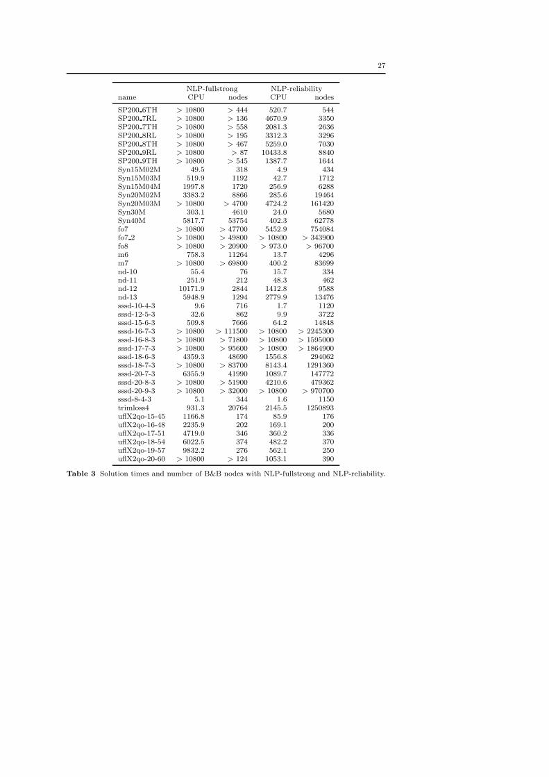
NLP-fullstrong NLP-reliabilityname CPU nodes CPU nodes

BatchS101006M 267.5 336 11.1 446BatchS121208M 1093.3 504 27.4 594BatchS151208M 3216.1 1310 114.9 2276BatchS201210M 3847.8 1122 176.8 2132CLay0204H 103.3 234 7.9 1143CLay0204M 9.0 224 0.7 1311CLay0205H 3441.6 2257 193.0 11191CLay0205M 220.2 1923 19.2 17934CLay0303M 0.9 35 0.8 784CLay0304H 90.2 117 191.7 11196CLay0304M 11.6 131 48.8 21942CLay0305H 4344.0 2318 252.0 11977CLay0305M 391.3 3096 19.8 16250FLay04H 133.6 652 38.9 2512FLay04M 4.7 618 1.6 2608FLay05H > 10800 > 11900 4686.0 101128FLay05M 290.7 15142 115.3 100838FLay06M > 10800 > 205800 9944.4 5477058RSyn0805M02M > 10800 > 1505 2363.0 43214RSyn0805M03M > 10800 > 593 7112.4 63848RSyn0820M > 10800 > 31400 1338.3 111676RSyn0830M > 10800 > 11800 2542.2 167782RSyn0830M03H > 10800 > 0 808.4 144RSyn0830M04H > 10800 > 0 3668.6 518RSyn0840M03H > 10800 > 0 1697.8 128RSyn0840M04H > 10800 > 0 4388.0 514SLay06H 136.8 92 3.9 99SLay06M 5.5 87 0.2 101SLay07H 492.3 126 11.8 196SLay07M 19.8 147 0.5 205SLay08H 1925.2 224 30.9 298SLay08M 67.9 229 1.1 259SLay09H 6623.2 323 68.5 395SLay09M 214.5 345 2.3 362SLay10H > 10800 > 0 1282.0 5486SLay10M 2200.8 1781 47.6 5787SP200 1RL > 10800 > 340 893.8 778SP200 1TH > 10800 > 489 825.6 1292SP200 2RL > 10800 > 56 > 10800 > 3900SP200 2TH > 10800 > 100 1848.1 2514SP200 3RL > 10800 > 125 1431.5 1668SP200 3TH > 10800 > 546 930.5 1289SP200 4RL > 10800 > 313 2477.6 3790SP200 5RL > 10800 > 99 4345.0 2325SP200 5TH > 10800 > 456 2360.8 3224SP200 6RL > 10800 > 179 4858.1 4294


27

NLP-fullstrong NLP-reliabilityname CPU nodes CPU nodes

SP200 6TH > 10800 > 444 520.7 544SP200 7RL > 10800 > 136 4670.9 3350SP200 7TH > 10800 > 558 2081.3 2636SP200 8RL > 10800 > 195 3312.3 3296SP200 8TH > 10800 > 467 5259.0 7030SP200 9RL > 10800 > 87 10433.8 8840SP200 9TH > 10800 > 545 1387.7 1644Syn15M02M 49.5 318 4.9 434Syn15M03M 519.9 1192 42.7 1712Syn15M04M 1997.8 1720 256.9 6288Syn20M02M 3383.2 8866 285.6 19464Syn20M03M > 10800 > 4700 4724.2 161420Syn30M 303.1 4610 24.0 5680Syn40M 5817.7 53754 402.3 62778fo7 > 10800 > 47700 5452.9 754084fo7 2 > 10800 > 49800 > 10800 > 343900fo8 > 10800 > 20900 > 973.0 > 96700m6 758.3 11264 13.7 4296m7 > 10800 > 69800 400.2 83699nd-10 55.4 76 15.7 334nd-11 251.9 212 48.3 462nd-12 10171.9 2844 1412.8 9588nd-13 5948.9 1294 2779.9 13476sssd-10-4-3 9.6 716 1.7 1120sssd-12-5-3 32.6 862 9.9 3722sssd-15-6-3 509.8 7666 64.2 14848sssd-16-7-3 > 10800 > 111500 > 10800 > 2245300sssd-16-8-3 > 10800 > 71800 > 10800 > 1595000sssd-17-7-3 > 10800 > 95600 > 10800 > 1864900sssd-18-6-3 4359.3 48690 1556.8 294062sssd-18-7-3 > 10800 > 83700 8143.4 1291360sssd-20-7-3 6355.9 41990 1089.7 147772sssd-20-8-3 > 10800 > 51900 4210.6 479362sssd-20-9-3 > 10800 > 32000 > 10800 > 970700sssd-8-4-3 5.1 344 1.6 1150trimloss4 931.3 20764 2145.5 1250893uflX2qo-15-45 1166.8 174 85.9 176uflX2qo-16-48 2235.9 202 169.1 200uflX2qo-17-51 4719.0 346 360.2 336uflX2qo-18-54 6022.5 374 482.2 370uflX2qo-19-57 9832.2 276 562.1 250uflX2qo-20-60 > 10800 > 124 1053.1 390

Table 3 Solution times and number of B&B nodes with NLP-fullstrong and NLP-reliability.

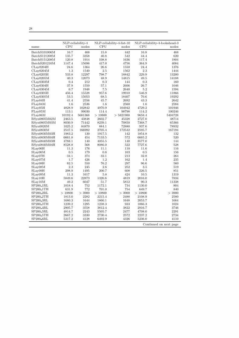
28

NLP-reliability-4 NLP-reliability-4-list-10 NLP-reliability-4-lookahead-3name CPU nodes CPU nodes CPU nodes

BatchS101006M 16.7 466 15.8 442 16.8 468BatchS121208M 135.7 3358 40.8 542 44.4 620BatchS151208M 120.8 1914 108.8 1636 117.4 1804BatchS201210M 1147.4 15696 417.0 4756 364.9 4084CLay0204H 24.6 1364 26.6 1550 24.4 1376CLay0204M 1.3 1540 2.5 1562 2.3 1444CLay0205H 533.8 12297 798.7 18842 229.9 13200CLay0205M 40.3 12073 48.9 14815 49.5 14188CLay0303M 0.4 212 0.3 144 0.3 160CLay0304H 37.9 1550 57.1 2606 26.7 1046CLay0304M 6.7 1948 7.5 2640 5.2 1594CLay0305H 456.4 15528 957.6 19910 546.9 11866CLay0305M 53.5 15053 68.5 18407 70.6 19292FLay04H 41.4 2556 45.7 2692 43.3 2642FLay04M 1.6 2536 1.6 2560 1.6 2584FLay05H 4828.9 102842 4970.9 104942 4729.2 101946FLay05M 113.1 99030 114.4 98798 114.2 100246FLay06M 10192.4 5681368 > 10800 > 5821900 9658.4 5404728RSyn0805M02M 2463.5 43848 2602.7 45328 2727.0 48714RSyn0805M03M 8030.9 71442 8239.1 70850 7368.7 65366RSyn0820M 1025.2 84870 884.1 72880 937.6 78932RSyn0830M 2547.5 166992 2705.4 172542 2595.7 167194RSyn0830M03H 1983.2 130 1917.5 142 1854.8 132RSyn0830M04H 6661.8 454 7133.5 572 6665.2 520RSyn0840M03H 4788.1 140 4055.5 140 3577.0 144RSyn0840M04H 8528.8 568 8086.0 522 7727.6 528SLay06H 11.3 176 11.1 110 11.6 116SLay06M 0.5 179 0.6 163 0.5 156SLay07H 34.1 374 32.1 213 32.8 264SLay07M 1.7 426 1.2 162 1.4 235SLay08H 82.5 550 76.2 297 96.6 560SLay08M 2.3 245 2.6 252 3.5 519SLay09H 298.9 1495 200.7 608 226.5 851SLay09M 11.3 1617 5.8 424 10.5 1319SLay10H 5849.6 22873 1326.6 4819 2016.0 7834SLay10M 49.2 6047 51.7 5812 90.3 11338SP200 1RL 1018.4 752 1172.1 734 1130.0 804SP200 1TH 631.9 772 701.0 754 649.7 840SP200 2RL > 10800 > 3900 > 10800 > 3900 > 10800 > 3900SP200 2TH 1813.0 2282 2215.4 2488 2108.9 2580SP200 3RL 1680.3 1644 1866.1 1648 2053.7 1664SP200 3TH 1239.2 1295 1238.3 933 1066.3 1024SP200 4RL 2905.7 3558 3812.4 3822 2916.7 3746SP200 5RL 4814.7 2243 5505.7 2477 4708.0 2291SP200 5TH 2667.2 3330 2730.4 2572 2237.2 2734SP200 6RL 5317.2 4128 6492.9 4326 5236.0 4110


29

NLP-reliability-4 NLP-reliability-4-list-10 NLP-reliability-4-lookahead-3name CPU nodes CPU nodes CPU nodes

SP200 6TH 744.8 548 836.2 428 700.0 460SP200 7RL 4608.6 3122 6379.2 3190 4771.0 3102SP200 7TH 2700.3 3554 2512.3 2621 2177.6 2569SP200 8RL 3852.9 3244 5057.4 3394 3809.6 3380SP200 8TH 4407.2 5526 4181.4 4026 4386.0 5130SP200 9RL 9844.3 8382 > 10800 > 3900 10209.7 8606SP200 9TH 1584.4 1738 1612.9 1560 1592.1 1692Syn15M02M 8.4 444 7.3 416 7.3 422Syn15M03M 52.9 1654 52.3 1712 49.5 1618Syn15M04M 276.6 6394 230.6 4914 249.5 5410Syn20M02M 306.9 21442 328.3 20844 332.5 21960Syn20M03M 4853.7 170968 4957.2 170142 5639.4 179566Syn30M 22.7 5260 23.8 5408 22.1 5050Syn40M 406.6 62518 386.9 58232 425.2 63030fo7 2807.2 430852 > 10800 > 1488800 3415.7 520406fo7 2 4266.7 531558 1137.4 163255 733.7 105658fo8 > 10800 > 991400 > 10800 > 874700 > 10800 > 823400m6 34.7 10398 68.4 20009 15.7 4751m7 1045.3 223058 307.6 60711 152.4 30946nd-10 17.1 262 20.0 326 19.5 314nd-11 55.2 458 57.2 466 55.9 450nd-12 1523.9 10050 1597.3 10674 1377.2 9492nd-13 2543.7 11652 3164.0 13604 2074.4 9052sssd-10-4-3 2.1 1160 3.2 2008 2.8 1736sssd-12-5-3 7.6 2400 9.7 3224 11.0 3570sssd-15-6-3 128.2 30072 86.5 20476 70.2 16278sssd-16-7-3 > 10800 > 2189100 585.1 116568 10040.7 2014152sssd-16-8-3 > 10800 > 1546400 > 10800 > 1617400 > 10800 > 1533700sssd-17-7-3 > 10800 > 1835200 2154.3 365816 8232.1 1450838sssd-18-6-3 5792.2 1088550 5410.4 1063808 2735.1 522384sssd-18-7-3 4437.0 693292 > 10800 > 1664600 8790.1 1311906sssd-20-7-3 2734.9 363620 691.4 93324 632.6 86976sssd-20-8-3 5706.6 645892 > 10800 > 1229900 > 10800 > 1195200sssd-20-9-3 > 10800 > 998000 > 10800 > 1021200 > 10800 > 974600sssd-8-4-3 2.0 1176 2.1 1226 1.6 832trimloss4 3235.2 1758206 3218.0 1701174 2494.9 1396042uflX2qo-15-45 141.6 174 140.9 174 144.9 180uflX2qo-16-48 258.9 202 259.4 202 263.1 204uflX2qo-17-51 479.8 332 482.7 336 489.8 334uflX2qo-18-54 667.9 374 649.3 390 652.3 376uflX2qo-19-57 894.5 244 906.1 272 898.0 264uflX2qo-20-60 1495.2 368 1521.6 388 1534.1 372

Table 4 Solution times and number of B&B nodes with NLP-reliability-4, NLP-reliability-4-list-10 and NLP-reliability-4-list-10-lookahead-3.

30

QP-fullstrong cold QP-fullstrong QP-reliabilityname CPU nodes CPU nodes CPU nodes

BatchS101006M 30.3 434 36.9 434 9.3 452BatchS121208M 90.3 560 117.4 560 23.8 616BatchS151208M 296.7 1444 380.4 1444 97.4 2000BatchS201210M 420.3 1446 524.0 1446 175.5 2236CLay0204H 20.2 806 23.2 801 7.5 1135CLay0204M 2.4 867 2.8 867 0.7 1314CLay0205H 485.9 4821 601.9 4928 192.8 11191CLay0205M 51.7 5478 64.2 5476 17.7 15596CLay0303M 1.1 564 1.2 608 1.6 1048CLay0304H 598.7 22056 661.2 21178 388.1 22026CLay0304M 95.9 22458 107.0 22640 41.7 19004CLay0305H 443.0 4826 604.9 4815 277.1 13984CLay0305M 79.6 5638 103.2 5638 18.4 16210FLay04H 39.0 1816 41.2 1824 38.5 2504FLay04M 1.7 1822 1.9 1822 1.6 2682FLay05H 3022.9 51532 3296.3 51756 4661.5 101146FLay05M 86.4 51038 97.8 51074 115.8 100852FLay06M 5309.1 2084902 6200.1 2081112 10556.3 5897892RSyn0805M02M 6030.7 36180 > 10800 > 23000 2323.1 42528RSyn0805M03M > 10800 > 18300 > 10800 > 6100 7584.3 66758RSyn0820M 1161.9 56448 2178.4 56448 1408.1 118062RSyn0830M 4427.2 134812 9175.5 134816 2463.6 162652RSyn0830M03H 503.4 130 951.5 132 345.3 138RSyn0830M04H 2037.9 283 3797.6 285 2364.0 510RSyn0840M03H 1064.8 144 1381.8 108 534.4 138RSyn0840M04H 3165.8 306 5812.2 307 2881.4 552SLay06H 8.9 84 9.8 84 2.8 114SLay06M 0.8 95 1.2 95 0.1 101SLay07H 27.0 134 29.8 127 8.9 200SLay07M 2.1 134 3.8 134 0.4 205SLay08H 97.3 223 106.1 223 22.8 276SLay08M 6.0 200 11.9 200 0.8 259SLay09H 313.6 341 341.6 330 57.0 393SLay09M 16.0 356 36.2 365 1.6 362SLay10H 3114.4 1754 3742.1 1751 1268.8 5486SLay10M 122.2 1772 346.1 1772 41.5 5787SP200 1RL 1175.5 1146 926.3 862 538.6 676SP200 1TH 611.6 658 554.1 658 434.3 864SP200 2RL 2743.9 1874 > 10800 > 4800 > 10800 > 3900SP200 2TH 3405.3 3046 3339.3 3046 1577.4 2622SP200 3RL 1062.3 658 1353.8 1590 1135.8 1694SP200 3TH 1016.5 1046 866.0 1046 798.8 1313SP200 4RL 2306.2 2450 2664.5 3730 2536.8 3804SP200 5RL 4810.9 1417 4798.2 2657 3455.9 2297SP200 5TH 2091.2 2216 2012.4 2216 2243.8 3220SP200 6RL 5061.6 3670 5420.3 4992 4541.1 4382


31

QP-fullstrong cold QP-fullstrong QP-reliabilityname CPU nodes CPU nodes CPU nodes

SP200 6TH 536.3 494 483.6 494 419.7 540SP200 7RL 4499.9 2046 4084.1 3136 4126.1 3378SP200 7TH 2269.2 2612 2200.3 2612 2330.2 3326SP200 8RL 2672.1 1808 4085.0 4078 2977.7 3310SP200 8TH 3889.9 4054 3608.8 4054 4764.3 7028SP200 9RL 2214.0 760 > 10800 > 8400 9793.0 8920SP200 9TH 1216.8 1524 1313.8 1524 1191.9 1684Syn15M02M 6.3 388 9.7 388 3.8 418Syn15M03M 48.4 1248 77.9 1248 37.6 1648Syn15M04M 250.9 3954 408.1 3954 284.7 7176Syn20M02M 404.7 16354 674.3 16354 345.9 23596Syn20M03M 5876.0 124108 10140.9 124108 4973.2 169328Syn30M 33.3 4880 50.6 4880 22.6 5398Syn40M 587.9 55228 887.3 55228 415.1 64984fo7 4490.4 385668 > 10800 > 239400 6432.9 886104fo7 2 2362.4 192554 2564.6 169086 > 10800 > 860100fo8 > 10800 > 401900 > 10800 > 289200 > 5328.9 > 450300m6 118.2 17518 175.1 20692 339.4 90110m7 2511.9 225436 2761.9 191716 663.8 139521nd-10 10.3 110 12.1 110 12.7 320nd-11 41.6 280 47.5 280 46.7 472nd-12 1707.7 5552 2002.6 5550 1397.6 9548nd-13 1326.9 3074 1433.0 3078 2752.9 13412sssd-10-4-3 1.5 678 1.8 668 1.4 1056sssd-12-5-3 2.9 624 3.6 594 13.2 5128sssd-15-6-3 57.4 8860 74.8 8694 48.3 11106sssd-16-7-3 4527.5 583408 6167.1 575306 > 10800 > 2279200sssd-16-8-3 4169.4 415102 6192.8 431732 > 10800 > 1594900sssd-17-7-3 1174.5 121728 1693.4 121998 > 10800 > 1836100sssd-18-6-3 546.4 73472 758.5 73532 1284.5 244742sssd-18-7-3 4587.7 461528 3643.5 263990 7590.0 1185160sssd-20-7-3 556.0 47100 803.6 47814 710.8 98820sssd-20-8-3 4823.5 338080 6910.8 337978 4971.0 565740sssd-20-9-3 > 10800 > 529800 > 10800 > 360400 > 10800 > 978600sssd-8-4-3 0.8 308 1.0 352 1.6 1228trimloss4 478.4 56419 526.7 61786 2459.7 1366666uflX2qo-15-45 184.9 174 198.0 174 72.0 176uflX2qo-16-48 322.0 202 333.8 202 137.1 200uflX2qo-17-51 688.9 352 735.3 352 316.3 336uflX2qo-18-54 901.0 388 976.0 388 409.5 368uflX2qo-19-57 1117.5 278 1211.8 278 467.8 250uflX2qo-20-60 2027.4 392 2138.4 392 896.2 390

Table 5 Solution times and number of B&B nodes with QP-fullstrong (with and withoutwarm starts) and QP-reliability.

32

LP-fullstrong Bonmin Hybridname CPU nodes CPU nodes

BatchS101006M 41.3 464 15.5 2012BatchS121208M 114.0 634 56.9 5856BatchS151208M 306.4 1458 64.8 7126BatchS201210M 401.8 1170 73.9 7462CLay0204H 15.5 526 7.1 1201CLay0204M 2.8 489 1.2 760CLay0205H 491.3 4366 80.1 11984CLay0205M 63.8 4576 11.6 7201CLay0303M 1.7 614 1.0 1074CLay0304H 646.1 22698 69.5 25258CLay0304M 111.5 22032 14.1 14882CLay0305H 360.2 4723 121.9 20616CLay0305M 90.7 5283 17.9 8034FLay04H 30.5 1162 7.3 2538FLay04M 2.1 1182 7.1 2242FLay05H 2483.0 43330 307.6 103328FLay05M 108.8 43202 80.9 77038FLay06M 6872.6 1709732 > 10800 > 3418713RSyn0805M02M 9147.7 77654 212.6 55870RSyn0805M03M > 10800 > 28200 135.1 15638RSyn0820M 1319.1 56820 7.4 3606RSyn0830M 5123.8 155972 4.4 1636RSyn0830M03H 411.7 138 32.3 62RSyn0830M04H 2349.9 442 72.9 324RSyn0840M03H 502.1 116 32.6 126RSyn0840M04H 2165.5 325 58.4 160SLay06H 8.9 138 26.2 1576SLay06M 1.5 103 1.8 370SLay07H 24.6 196 132.5 13022SLay07M 5.4 360 4.0 2430SLay08H 102.9 568 217.3 11362SLay08M 10.9 255 9.8 4362SLay09H 179.3 454 1180.5 104126SLay09M 29.1 668 47.5 23010SLay10H 5058.8 9297 > 10800 > 744043SLay10M 665.9 9129 509.8 221578SP200 1RL 5651.9 4922 > 10800 > 1219551SP200 1TH 2931.0 4266 > 10800 > 877437SP200 2RL > 10800 > 8300 > 10800 > 1641695SP200 2TH 8105.2 9086 > 10800 > 606517SP200 3RL > 10800 > 3900 > 10800 > 1074241SP200 3TH 2783.2 3334 > 10800 > 570829SP200 4RL 7924.2 8882 > 10800 > 1261129SP200 5RL > 10800 > 3900 > 10800 > 1106807SP200 5TH 7543.8 9748 > 10800 > 686015SP200 6RL > 10800 > 3900 > 10800 > 1201837


33

LP-fullstrong Bonmin Hybridname CPU nodes CPU nodes

SP200 6TH 2274.5 2740 > 10800 > 634600SP200 7RL > 10800 > 3900 > 10800 > 1126801SP200 7TH 5131.6 6971 > 10800 > 681875SP200 8RL > 10800 > 7900 > 10800 > 1137771SP200 8TH 9888.4 12462 > 10800 > 638302SP200 9RL > 10800 > 3900 > 10800 > 1247269SP200 9TH 3915.2 4982 > 10800 > 834099Syn15M02M 6.6 310 0.2 0Syn15M03M 46.6 930 1.1 30Syn15M04M 164.3 1840 2.1 106Syn20M02M 335.7 9320 0.8 98Syn20M03M 4833.6 72012 1.3 44Syn30M 39.8 5114 0.2 36fo7 5394.3 297670 320.1 249178fo7 2 2526.4 125582 214.7 179242fo8 > 10800 > 301900 567.0 414508m6 147.9 12984 52.4 57786m7 1666.7 87530 84.0 77236nd-10 9.1 100 2.8 434nd-11 37.0 240 5.2 710nd-12 1163.8 4210 69.0 15360nd-13 839.9 2050 93.5 18006sssd-10-4-3 5.5 2490 1.3 1646sssd-12-5-3 22.1 5564 29.4 50476sssd-15-6-3 256.0 41562 7407.0 4865798sssd-16-7-3 9617.5 1350244 > 10800 > 4482231sssd-16-8-3 > 10800 > 1073600 > 10800 > 5418301sssd-17-7-3 2146.5 271570 > 10800 > 5166701sssd-18-6-3 4016.5 561284 461.9 556350sssd-18-7-3 > 10800 > 1110200 > 10800 > 4487101sssd-20-7-3 > 10800 > 1036700 > 10800 > 4857701sssd-20-8-3 > 10800 > 877100 > 10800 > 5122301sssd-20-9-3 > 10800 > 693700 > 10800 > 4962121sssd-8-4-3 2.5 1218 1.0 706trimloss4 528.8 55350 746.9 444832uflX2qo-15-45 82.4 186 55.5 2290uflX2qo-16-48 162.1 230 295.8 9808uflX2qo-17-51 318.3 326 236.9 7052uflX2qo-18-54 472.8 358 953.8 22050uflX2qo-19-57 485.5 246 2005.1 43596uflX2qo-20-60 863.9 360 2937.8 55514

Table 6 Solution times and number of B&B nodes with LP-fullstrong and Bonmin Hybridalgorithm.

More Branch-and-Bound Experiments in Convex Nonlinear ...More Branch-and-Bound Experiments in Convex...

Documents

Transcript of More Branch-and-Bound Experiments in Convex Nonlinear ...More Branch-and-Bound Experiments in Convex...