On the Cost of Unsuccessful Searches in Search Trees with

Two-way Comparisons

Marek Chrobak∗ Mordecai Golin† J. Ian Munro‡ Neal E. Young§

March 10, 2021

Abstract

Search trees are commonly used to implement access operations to a set of stored keys. Ifthis set is static and the probabilities of membership queries are known in advance, then one canprecompute an optimal search tree, namely one that minimizes the expected access cost. For anon-key query, a search tree can determine its approximate location by returning the inter-keyinterval containing the query. This is in contrast to other dictionary data structures, like hashtables, that only report a failed search. We address the question “what is the additional cost ofdetermining approximate locations for non-key queries”? We prove that for two-way comparisontrees this additional cost is at most 1. Our proof is based on a novel probabilistic argumentthat involves converting a search tree that does not identify non-key queries into a random treethat does.

1 Introduction

Search trees are among the most fundamental data structures in computer science. They are usedto store a collection of values, called keys, and allow efficient access and updates. The most commonoperations on such trees are search queries, where a search for a given query value q needs to returnthe pointer to the node representing q, provided that q is among the stored keys.

In scenarios where the keys and the probabilities of all potential queries are fixed and knownin advance, one can use a static search tree, optimized so that its expected cost for processingsearch queries is minimized. These trees have been studied since the 1960s, including a classic workby Knuth [16] who developed an O(n2) dynamic programming algorithm for trees with three-waycomparisons (3wcst’s). A three-way comparison “q : k” between a query value q and a key k hasthree possible outcomes: q < k, q = k, or q > k, and thus it may require two comparisons, namely“q = k” and “q < k”, when implemented in a high-level programming language. This was in factpointed out by Knuth himself in the second edition of “The Art of Computer Programming” [17,§6.2.2 ex. 33]. It would be more efficient to have each comparison in the tree correspond to just

∗University of California at Riverside. Research supported by NSF grants CCF-1217314 and CCF-1536026†Hong Kong University of Science and Technology. Research funded by HKUST/RGC grant FSGRF14EG28 and

RGC CERG Grant 16208415.‡University of Waterloo. Research funded by NSERC Discovery Grant 8237-2012 and the Canada Research Chairs

Programme.§University of California at Riverside. Research supported by NSF grant IIS-1619463.

1

arX

iv:2

103.

0105

2v2

[cs

.DS]

9 M

ar 2

021

one binary comparison. Nevertheless, trees with two-way comparisons (2wcst’s) are not as wellunderstood as 3wcst’s, and the fastest algorithm for computing such optimal trees runs in timeΘ(n4) [2, 4, 6, 7].

Queries for keys stored in the tree are referred to in the literature as successful queries, whilequeries for non-key values are unsuccessful. Every 3wcst inherently supports both types of queries.The search for a non-key query q in a 3wcst determines the “location” of q — the inter-key intervalcontaining q. (By an inter-key interval we mean an inclusion-maximal open interval not containingany key.) Equivalently, it returns q’s successor in the key set (if any). This feature is a by-productof 3-way comparisons — even if this information is not needed, the search for q in a 3wcst producesthis information at no additional cost. In contrast, other commonly used dictionary data structures(such as hash tables) provide only one bit of information for non-key queries — that the query isnot a key. This suffices for some applications, for example in parsing, where one needs to efficientlyidentify keywords of a programming language. In other applications, however, returning the non-key query interval (equivalently, the successor) is useful. For example, when search values areperturbed keys (say, obtained from inaccurate measurements), identifying the keys nearest to thequery may be important.

With this in mind, it is reasonable to consider two variants of 2wcst’s: 2wcstloc’s, whichare two-way comparison search trees that return the inter-key interval of each non-key query (justlike 3wcst’s), and 2wcstnil’s, that only return the “not a key” value ⊥ to report unsuccessfulsearch (analogous to hash tables). Since 2wcstnil trees provide less information, they can costless than 2wcstloc’s. To see why, consider an example (see Figure 1) with keys K = 1, 2, eachwith probability 1/5. Inter-key intervals (−∞, 1), (1, 2), (2,∞) each have probability 1/5 as well.The optimum 2wcstloc tree (which must determine the inter-key interval of each non-key query),has cost 12/5, while the optimum 2wcstnil tree (which need only identify non-keys as such) hascost 9/5. Note that 2wcstloc trees are much more constrained; they contain exactly 2n+ 1 leaves.2wcstnil trees may contain between n + 1 and 2n + 1 leaves. (More precisely, these statementshold for non-redundant trees — see Section 2.)

To our knowledge, the first systematic study of 2wcst’s was conducted by Spuler [21, 22], whosedefinition matches our definition of 2wcstnil’s. Prior to that work, Andersson [3] presented someexperimental results in which using two-way comparisons improved performance. Earlier, variousother types of search trees called split trees, which are essentially restricted variants of 2wcst’s,were studied in [20, 15, 19, 12, 14]. (As pointed out in [5], the results in [21, 22, 14] contain somefundamental errors.)

Our contribution. The discussion above leads naturally to the following question: “for two-waycomparison search trees, what is the additional cost of returning locations for all non-key queries”?We prove that this additional cost is at most 1. Specifically (Theorem 1 in Section 3), for any2wcstnil T

∗ there is a 2wcstloc T′ solving the same instance, such that the (expected) cost of a

query in T ′ is at most 1 more than in T ∗. We find this result to be somewhat counter-intuitive,since, as illustrated in Figure 1, a leaf in a 2wcstnil may represent queries from multiple (perhapseven all) inter-query intervals, so in the corresponding 2wcstloc it needs to be split into multipleleaves by adding inequality comparisons, which can significantly increase the tree depth. The proofuses a probabilistic construction that converts T ∗ into a random 2wcstloc T

′, increasing the depthof each leaf by at most one in expectation.

The bound in Theorem 1 is tight. To see why, consider an example with just one key 1 whoseprobability is ε ∈ (0, 12) and inter-key intervals (−∞, 1) and (1,∞) having probabilities ε and 1−2ε,

2

q < 2

2

q = 2

(2,+∞)

1/5 1/5 1/5

q < 1

q = 1

1 (1,2)

1/5 1/5

(-∞,1)

n

n

n ny

y

y

y

q = 1

1

2

q = 2

⊥

1/5

1/5 3/5

y n

ny

Figure 1: Identifying non-keys can cost more. In this example, all keys and inter-key intervals haveprobability 1

5 . The cost of the 2wcstnil on the left is 1 · 15 + 2 · 15 + 2 · 35 = 95 . The cost of the

2wcstloc on the right is 2 · 15 + 3 · 15 + 3 · 15 + 2 · 15 + 2 · 15 = 125 . We use the standard convention

for graphical representation of search trees, with queries in the internal nodes, and with searchproceeding to the left child if the answer to the query is “yes” and to the right child if the answeris “no”.

respectively. The optimum 2wcstnil has cost 1, while the optimum 2wcstloc has cost 2−ε. Takingε arbitrarily close to 0 establishes the gap. (As in the rest of the paper, in this example the allowedcomparisons are “=” and “<”, but see the discussion in Section 5.)

Successful-only model. Many authors have considered successful-only models, in which the treessupport key queries but not non-key queries. For 3wcst’s, Knuth’s algorithm [16] can be usedfor both the all-query and successful-only variants. For 2wcst’s, in successful-only models thedistinction between 2wcstloc and 2wcstnil does not arise. Alphabetic trees can be considered as2wcst trees, in the successful-only model, restricted to using only “<” comparisons. They can bebuilt in O(n log n) time [13, 10]. Anderson et al. [2] gave an O(n4)-time algorithm for successful-only2wcst’s that use “<” and “=” comparisons. With some effort, their algorithm can be extended tohandle non-key queries too. A simpler and equally fast algorithm, handling all variants of 2wcst’s(successful only, 2wcstnil, or 2wcstloc’s) was recently described in [7].

Application to entropy bounds. For most types of two-way comparison search trees, the entropyof the distribution is a lower bound on the optimum cost. This bound has been widely used,for example to analyze approximation algorithms (e.g. [18, 23, 4, 6]). Its applicability to “20-Questions”-style games (closely related to constructing 2wcst’s) was recently studied by Dagal etal. [8, 9]. But the entropy bound does not apply directly to 2wcstnil’s. Section 4 explains why,and how, with Theorem 1, it can be applied to such trees.

Other gap bounds. To our knowledge, the gap between 2wcstloc’s and 2wcstnil’s has not pre-viously been considered. But gaps between other classes of search trees have been studied. An-dersson [3] observed that for any depth-d 3wcst, there is an equivalent 2wcstloc of depth atmost d + 1. Gilbert and Moore [11] showed that for any successful-only 2wcst (using arbitrarybinary comparisons), there is one using only “<” comparisons that costs at most 2 more. This wasimproved slightly by Yeung [23]. Anderson et al. [2, Theorem 11] showed that for any successful-only 2wcst that uses “<” and “=” comparisons, there is one using only “<” comparisons thatcosts at most 1 more. Chrobak et al. [4, 6, Theorem 2] leveraged Yeung’s result to show that forany 2wcstloc (of any kind, using arbitrary binary comparisons) there is one using only “<” and“=” comparisons that costs at most 3 more. The trees guaranteed to exist by the gap bounds

3

in [11, 23, 2, 4, 6] can be computed in O(n log n) time, whereas the fastest algorithms known forcomputing their optimal counterparts take time Θ(n4).

2 Preliminaries

Without loss of generality, throughout the paper assume that the set of keys is K = 1, 2, . . . , n(with n ≥ 0) and that all queries are from the open interval U = (0, n+ 1).

In a 2wcstloc T each internal node represents a comparison between the query value, denotedby q, and a key k ∈ K. There are two types of comparison nodes: equality comparison nodes〈q= k〉, and inequality comparison nodes 〈q <k〉. Each comparison node in T has two children, oneleft and one right, that correspond to the “yes” and “no” outcomes of the comparison, respectively.For each key k there is a leaf k in T and for each i ∈ 0, 1, . . . , n there is a leaf identified byopen interval (i, i+ 1). For any node N of T , the subtree of T rooted at N (that is, induced by Nand its descendants) is denoted TN .

Consider a query q ∈ U . A search for q in a 2wcstloc T starts at the root node of T and followsa path from the root towards a leaf. At each step, if the current node is a comparison 〈q= k〉 or〈q <k〉, if the outcome is “yes” then the search proceeds to the left child, otherwise it proceeds tothe right child. A tree is correct if each query q ∈ U reaches a leaf ` such that q ∈ `. Note that ina 2wcstloc there must be a comparison node 〈q= k〉 for each key k ∈ K.

The input is specified by a probability distribution (α, β) on queries, where, for each key k ∈ K,the probability that q = k is βk and for each i ∈ 0, 1, . . . , n the probability that q ∈ (i, i + 1)is αi. As the set of queries is fixed, the instance is uniquely determined by (α, β). The cost of agiven query q is the number of comparisons in a search for q in T , and the cost of tree T , denotedcost(T ), is the expected cost of a random query q. (Naturally, cost(T ) depends on (α, β), but theinstance is always understood from context, so is omitted from the notation.) More specifically,for any query q ∈ U , let depthT (q) denote the query depth of q in T — the number of comparisonsmade by a search in T for q. Then cost(T ) is the expected value of depthT (q), where random queryq is chosen according to the query distribution (α, β).

The definition of 2wcstnil’s is similar to 2wcstloc’s. The only difference is that non-key leavesdo not represent the inter-key interval of the query: in a 2wcstnil, each leaf either represents a keyk as before, or is marked with the special symbol ⊥, representing any non-key query. A 2wcstnil

may have multiple leaves marked ⊥, and searches for queries in different inter-key intervals mayterminate at the same leaf.

Also, the above definitions permit any key (or inter-key interval, for 2wcstloc’s) to have morethan one associated leaf, in which case the tree is redundant. Formally, for any node N , denote byUN the set of query values whose search reaches N . (For the root, UN = U .) Call a node N ofT redundant if UN = ∅. Define tree T to be redundant if it contains at least one redundant node.There is always an optimal tree that is non-redundant: any redundant tree T can be made non-redundant, without increasing cost, by splicing out parents of redundant nodes. (If N is redundant,replace its parent M by the sibling of N , removing M and TN .) But in the proof of Theorem 1 itis technically useful to allow redundant trees.

For any non-redundant 2wcstloc tree T , the cost is conventionally expressed in terms of leafweights: each key leaf N = k has weight wN = βk, while each non-key leaf N = (i, i+ 1) hasweight wN = αi. In this notation, letting leaves(T ) denote the set of leaves of T and depthT (N)

4

denote the depth of a node N in T ,

cost(T ) =∑

L∈ leaves(T )

wL · depthT (L). (1)

But the proof of Theorem 1 uses only the earlier definition of cost, which applies in all cases(redundant or non-redundant, 2wcstloc or 2wcstnil).

3 The Gap Bound

This section proves Theorem 1, that the additional cost of returning locations of non-key queriesis at most 1. The proof uses a probabilistic construction that converts any 2wcstnil (a tree thatdoes not identify locations of unsuccessful queries) into a random 2wcstloc (a tree that does). Theconversion increases the depth of each leaf by at most 1 in expectation, so increases the tree costby at most 1 in expectation.

Theorem 1. Fix some instance (α, β). For any 2wcstnil tree T ∗ for (α, β) there is a 2wcstloc

tree T ′ for (α, β) such that cost(T ′) ≤ cost(T ∗) + 1.

Proof. Let T ∗ be a given 2wcstnil. Without loss of generality assume that T ∗ is non-redundant.We describe a randomized algorithm that converts T ∗ into a random 2wcstloc tree T ′ for (α, β)with expected cost E[cost(T ′)] ≤ cost(T ∗) + 1. Since the average cost of a random tree T ′ satisfiesthis inequality, some 2wcstloc tree T ′′ must exist satisfying cost(T ′′) ≤ cost(T ∗) + 1, proving thetheorem. Our conversion algorithm starts with T = T ∗ and then gradually modifies T , processingit bottom-up, and eventually produces T ′.

For any key k ∈ K, let `k denote the unique ⊥-leaf at which a search for k starting in theno-child of 〈q= k〉 would end. Say that a leaf ` has a break due to k if k separates the query set U`of `; that is, ∃q, q′ ∈ U` with q < k < q′. Note that `k is the only leaf in the tree that can have abreak due to k.

In essence, the algorithm converts T ∗ into a (random) 2wcstloc tree T ′ by removing the breaksone by one. For each equality test 〈q= k〉 in T ∗, the algorithm adds one less-than comparison node〈q <k〉 near 〈q= k〉 to remove any potential break in `k due to k. (Here, by “near” we mean thatthis new node becomes either the parent or a child or a grandchild of 〈q= k〉.) This can increasethe depth of some leaves. The algorithm adds these new nodes in such a way that, in expectation,each leaf’s depth will increase by at most 1 during the whole process. In the end, if ` is a ⊥-leafthat does not have any breaks, then U` represents an inter-key interval. (Here we also use theassumption that T ∗ is non-redundant.) Thus, once we remove all breaks from ⊥-leaves, we obtaina 2wcstloc tree T ′.

To build some intuition before we dive into a formal argument, let’s consider a node N = 〈q=B〉,where B is a key, and suppose that leaf `B has a break due to B. The left child of N is leaf B, andlet t denote the right subtree of N . We can modify the tree by creating a new node N ′ = 〈q <B〉,making it the right child of N , with left and right subtrees of N ′ being copies of t (from whichredundant nodes can be removed). This will split `B into two copies and remove the break dueto `B, as desired. Unfortunately, this simple transformation also can increase the depth of someleaves, and thus also the cost of the tree.

In order to avoid this increase of depth, our tree modifications also involve some local rebalancingthat compensates for adding an additional node. The example above will be handled using a case

5

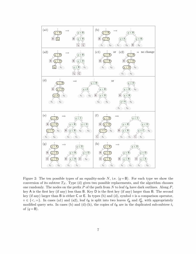
analysis. As one case, suppose that the root of t is a comparison nodeM = 〈q A〉, where ∈ <,=is any comparison operator and A is a key smaller than B. Denote by t1 and t2 the left and rightsubtrees of M . Our local transformation for this case is shown in Figure 2(b). It also introducesN ′ = 〈q <B〉, as before, but makes it the parent of N . Its left subtree is M , whose left and rightsubtrees are t1 and a copy of t2. Its right subtree is N , whose right subtree is a copy of t2. As canbe easily seen, this modification does not change the depth of any leaves except for `B. It is alsocorrect, because in the original tree a search for any query r ≥ B that reaches N cannot descendinto t1.

The full algorithm described below breaks the problem into multiple cases. Roughly, in caseswhen `B is deep enough in the subtree T ∗N of T ∗ rooted at N , we show that T ∗N can be rebalancedafter splitting `B. Only when `B is close to N we might need to increase the depth of T ∗N .

Conversion algorithm. The algorithm processes all nodes in T ∗ bottom-up, via a post-order nodetraversal, doing a conversion step Convert(N) on each equality-test node N of T ∗. (Post-ordertraversal is necessary for the proof of correctness and analysis of cost.) More formally, the algorithmstarts with T = T ∗ and executes Process(T ), where Process(TN ) is a recursive procedure thatmodifies the subtree rooted at node N in the current tree T as follows:

Process(TN ):For each child N2 of N , do Process(TN2).If N is an equality-test node, Convert(N).

(By definition, if N is a leaf then Process(TN ) does nothing.)

Procedure Process() will create copies of some subtrees and, as a result, it will also createredundant nodes in T . This might seem unnatural and wasteful, but it streamlines the descriptionof the algorithm and the proof. Once we construct the final tree T ′, these redundant nodes can beremoved from T ′ following the method outlined in Section 2.

Subroutine Convert(N), where N is an equality-test node 〈q=B〉, has three steps:

1. Consider the path from N to `B. Let P be the prefix of this path that starts at N andcontinues just until P contains either

(i) the leaf `B, or

(ii) a second comparison to key B, or

(iii) any comparison to a key smaller than B, or

(iv) two comparisons to keys (possibly equal) larger than B.

Thus, prefix P contains N and at most two other nodes. In case (iii), the last node on Pwith comparison to a key smaller than B will be denoted 〈q A〉, where ∈ =, < is thecomparison operation and A is this key. If P has a comparison to a key larger than B, denotethe first such key by D; if there is a second such key, denote it C if smaller than D, or E iflarger.

2. Next, determine the type of N . The type of N is whichever of the ten cases (a1)-(h) in Fig. 2matches prefix P . (We show below that one of the ten must match P .)

3. Having identified the type of N , replace the subtree TN rooted at N (in place) by the re-placement for its type from Fig. 2.

6

(a1)q = B

B `B

q = B

B q < B

`′B `′′B

yn

yn

y n

=⇒ (b)q = B

B q A

t1 t2

q < B

q A

t1 t2

q = B

B t2

yn

y n

y

y n

n

yn

=⇒

(a2)q = B

B q < D

`B t1

q = B

B q < D

q < B

`′B `′′B

t1

yn

y n

yn

y

y n

n

=⇒ (c1)q = B

B q < B

t1 t2

(c2)q = B

B q < D

q < B

t1 t2

t3

yn

y n

yn

y

y n

n

or ⇒ no change

(d)q = B

B q < D

q A

t1 t2

t3

q < B

q A

t1 t2

q = B

B q < D

t2 t3

q < D

q = B

B q < B

q A

t1 t2

t2

t3

yn

y

y n

n

y

y n

n

yn

y n

y

yn

y

y n

n

n

=⇒ or

(e)q = B

B q < D

q < C

t1 t2

t3

q < C

q = B

B q < B

t1 t1

q < D

t2 t3

yn

y

y n

n

y

yn

y n

n

y n

=⇒ (f)q = B

B q < D

q = C

C t1

t2

q < C

q = B

B q < B

t1 t1

q < D

q = C

C t1

t2

yn

y

yn

n

y

yn

y n

n

y

yn

n

=⇒

(g)q = B

B q = D

D q < D

t1 t2

q < D

q = B

B q < B

t1 t1

q = D

D t2

yn

yn

y n

y

yn

y n

n

yn

=⇒ (h)q = B

B q = D

D q < E

t1 t2

q < D

q = B

B q < B

t1 t1

q = D

D q < E

t1 t2

yn

yn

y n

y

yn

y n

n

yn

y n

=⇒

Figure 2: The ten possible types of an equality-node N , i.e. 〈q=B〉. For each type we show theconversion of its subtree TN . Type (d) gives two possible replacements, and the algorithm choosesone randomly. The nodes on the prefix P of the path from N to leaf `B have dark outlines. Along P ,key A is the first key (if any) less than B. Key D is the first key (if any) larger than B. The secondkey (if any) larger than B is either C or E. In types (b) and (d), symbol is a comparison operator, ∈ <,=. In cases (a1) and (a2), leaf `B is split into two leaves `′B and `′′B, with appropriatelymodified query sets. In cases (b) and (d)-(h), the copies of `B are in the duplicated sub-subtree tiof 〈q=B〉.

7

For example, N is of type (b) if the second node N2 on P does a comparison to a key less thanB; therefore, as described in (1) (iii) above, N2 is of the form 〈q A〉. For type (b), the new subtreesplits P by adding a new comparison node 〈q <B〉, with yes-child N2 and no-child N , with subtreescopied appropriately from TN . (These trees are copied as they are, without removing redundancies.So after the reduction the tree will have two identical copies of t2.) For type (d), there are twopossible choices for the replacement subtree. In this case, the algorithm chooses one of the twouniformly at random.

Intuitively, the effect of each conversion in Fig. 2 is that leaf `B gets split into two leaves, onecontaining the queries smaller than B and the other containing the queries larger than B. This isexplicit in cases (a1) and (a2) where these two new leaves are denoted `′B and `′′B, and is implicitin the remaining cases. The two leaves resulting from the split may still contain other breaks, forkeys of equality tests above N . (If it so happens that B equals min U`B or max U`B , meaning thatB is not actually a break, then the query set of one of the resulting leaves will be empty.)

This defines the algorithm. Let T ′ = Process(T ∗) denote the random tree it outputs. Asexplained earlier, T ′ may be redundant.

Correctness of the algorithm. By inspection, Convert(N) maintains correctness of the tree whileremoving the break for N ’s key B, without introducing any new breaks. Hence, provided thealgorithm completes successfully, the tree T ′ that it outputs is a correct tree. To complete theproof of correctness, we prove the following claim.

Claim 2. In each call to Convert, some conversion (a1)-(h) applies.

Proof. Consider the time just before Step (3) of Convert(N). Let key B, subtree TN , and pathP be as defined for steps (1)–(3) in converting N . Recall that N is 〈q=B〉. Assume inductivelythat each equality-test descendant of N , when converted, had one of the ten types. Let N2 be thesecond node on P , N ’s no-child. Let N3 be the third node, if any. We consider a number of cases.

Case 1. N2 is a leaf: Then N is of type (a1).

Case 2. N2 is a comparison node with key less than B: Then N is of type (b).

Case 3. N2 is a comparison node with key B: Then N2 cannot do an equality test to B, becauseN does that, the initial tree was irreducible, and no conversion introduces a new equality test. SoN is of type (c1).

Case 4. N2 is a comparison node with key larger than B: Denote N2’s key by D. In this case Phas three nodes. There are two sub-cases:

Case 4.1. N2 does a less-than test (N2 is 〈q <D〉): By definition of P and `B, the yes-child ofN2 is the third node N3 on P . If N3 is a leaf, then N is of type (a2). Otherwise N3 is acomparison node. If N3’s key is smaller than B, then N is of type (d). If N3’s key is B, then Nis of type (c2). (This is because B has at most one equality node in TN , as explained in Case 3.)If N3’s key is larger than B and less than D, then N is of type (e) or (f).

To finish Case 4.1, we claim that N3’s key cannot be D or larger. Suppose otherwise forcontradiction. Let N3 be 〈q D′〉, where D′ ≥ D. By inspection of each conversion type, noconversion produces an inequality root whose yes-child has larger key, so N2 was not producedby a previous conversion. So N2 was in the original tree T ∗, where, furthermore, N2’s yes-subtreecontained a node with the key D′. (This holds whether N3 itself was in T ∗, or N3 was producedby some conversion, as no conversion adds new comparison keys to its subtree.) This contradictsthe irreducibility of T ∗, proving the claim.

8

Case 4.2. N2 does an equality test (N2 is 〈q=D〉): By the recursive nature of Process(), thetree rooted at N2 must be the result of applying Process() to the earlier no-child of N =〈q=B〉. Further it must be the result of a Convert() operation (since Process() of an inequalitycomparison just returns that inequality comparison as root). Consider the previous conversionthat producedN2. Inspecting the conversion types, the only conversions that could have producedN2 (with equality test at the root) are types (a1), (a2), (c1), and (c2). Each such conversionproduces a subtree TN2 where N2’s no-child does some less-than test 〈q <X〉 to a key at least aslarge as the key of the root, that is X ≥ D. This node is now N3.

So, if X = D, then N is of type (g), while if X > D, then N is of type (h).

In summary, we have shown that at each step of our algorithm at least one of the cases in Fig. 2applies. This completes the proof of Claim 2.

Cost estimate. Continuing the proof of Theorem 1, we now estimate the cost of T ′, the random treeproduced by the algorithm. To prove E[cost(T ′)] ≤ cost(T ∗) +1, we prove that, in expectation, thecost of each query r increases by at most 1. More precisely, we prove that for every query r ∈ U ,we have E[depthT ′(r)] ≤ depthT ∗(r) + 1.

Fix any query r ∈ U . We distinguish two cases, depending on whether r is a key or not.

Case 1. r ∈ K: Then key r has one equality node 〈q= r〉 in T ∗. By inspection, each conversion (b)or (d)-(h) increases the query depth of the key B of converted node 〈q=B〉 (i.e., N) by 1, and, inexpectation, does not increase any other query depth. For example, consider a conversion of type(d). The depth of the root of subtree t1 either increases by one or decreases by one, and, sinceeach is equally likely, is unchanged in expectation. Likewise for t3 and the first copy of t2. Thedepth of the root of the second copy of t2 is unchanged. Also, the queries r that descend into t2in TN can be partitioned into those smaller than B, and those larger. For either random choice ofreplacement subtree, the former descend into the first copy of t2, the latter descend into the secondcopy. Hence, in expectation, if r = B then this conversion increases the query depth of r by atmost 1, and if r ∈ U − B then r’s query depth does not increase.

By inspection of the two remaining conversion types, (a1) and (a2), each of those increases thedepth of the queries in `B’s query set by 1, without increasing the query depth of any other query.Since r ∈ K, query r is not in leaf `B for any such conversion. Hence, conversions (a1) and (a2)don’t increase r’s query depth.

So at most one conversion step in the entire sequence can increase r’s query depth (in expecta-tion) — the conversion whose root is the equality-test node for r, which increases the query depthby at most 1. It follows that the entire sequence increases the query depth of r by at most 1 inexpectation.

Case 2. r 6∈ K: In this case, r has no equality node in T ∗. As observed in Case 1, the only conversionstep that can increase the query depth of r (in expectation) is an (a1) or (a2) conversion of a node〈q=B〉 where `B is r’s leaf (that is, r ∈ U`). This step increases r’s query depth by 1.

So consider the tree just before such a conversion step applied to the subtree TN , where case (a1)or (a2) is applied and r’s leaf is `B. We show the following property holds at that time:

Claim 3. There was no earlier step whose conversion subtree contained the leaf of r.

Proof. To justify this claim, we consider cases (a1) and (a2) separately. For case (a1), r’s leafhas no processed ancestors. (A “processed” node is any node in the replacement subtree of any

9

previously implemented conversion.) But there is no conversion type that produces such a leaf,proving the claim in this case. The argument in case (a2) is a bit less obvious but similar: in thiscase r’s leaf is a yes-child and its parent is an inequality node that is the only processed ancestorof this leaf. By inspection of each conversion type, for each conversion that produces a leaf withonly one processed ancestor (which would necessarily be the root for the converted subtree), thisancestor is either an equality test (cases (a1), (a2), (c1), (c2)), or has this leaf be a no-child of itsparent (the second option of case (d), with t3 being a leaf). Thus no such conversion can producea subtree of type (a2) with r’s leaf being `B, completing the proof of the claim.

We then conclude that in this case (r 6∈ K), there is at most one step in which the expectedquery depth of r can increase; and if it does, it increases only by 1, so the total increase of r’s querydepth is at most 1 in expectation.

Summarizing, in either Case 1 or 2, the entire sequence of operations increases r’s query depthby at most one in expectation (with respect to the random choices of the algorithm), that isE[depthT ′(r)] ≤ depthT ∗(r) + 1. Since this property holds for any r ∈ U , applying linearity ofexpectation (and using depthT ((i, i+ 1)) to represent the depth in T of queries in inter-key interval(i, i+ 1)),

E[cost(T ′)] = E[∑n

i=1 βi depthT ′(i) +∑n

i=0 αi depthT ′((i, i+ 1))]

=∑n

i=1 βiE[depthT ′(i)] +∑n

i=0 αiE[depthT ′((i, i+ 1))]

≤∑n

i=1 βi(1 + depthT ∗(i)) +∑n

i=0 αi(1 + depthT ∗((i, i+ 1)))

= 1 + cost(T ∗).

This completes the proof of Theorem 1.

4 Application To Entropy Bounds

In general, a search tree determines the answer to a query from a set of some number m of possibleanswers. In the successful-only model there are n possible answers, namely the key values. In thegeneral 2wcstloc model there are 2n+1 answers: the n key values and the n+1 inter-key intervals.In the 2wcstnil model there are n + 1 answers: the n key values and ⊥. Let p be a probabilitydistribution on the m answers, namely pj is the probability that the answer to a random queryshould be the jth answer. It is well-known that any binary-comparison search tree T that returnssuch answers in its leaves satisfies cost(T ) ≥ H(p), where H(p) =

∑j pj log2

1pj

is the Shannon

entropy of p. This fact is a main tool used for lower bounding the optimal cost of search trees [1].The entropy bound can be weak when applied directly to 2wcstnil’s. To see why, consider a

probability distribution (α, β) on keys and inter-key intervals. Since 2wcstnil’s do not actuallyidentify inter-key intervals, the answers associated with a 2wcstnil are the key values and the⊥ symbol representing the “not a key” answer, so the corresponding distribution is (A, β), forA =

∑i αi. Thus the entropy lower bound is

cost(T ∗) ≥ H(A, β) = A log21

A+∑i

βi log21

βi

10

for any 2wcstnil tree T ∗. On the other hand, by Theorem 1, cost(T ∗) ≥ cost(T ′) − 1 for some2wcstloc tree T ′. The entropy lower bound cost(T ′) ≥ H(α, β) applies to T ′, giving the followinglower bound:

Corollary 4. For any 2wcstnil tree T ∗ for any input (α, β), cost(T ∗) ≥ H(α, β)− 1.

To see that this bound can be stronger, consider the following extreme example. Suppose thatβk = 1/n2 for all k, and that αi = 1

n+1

(1− 1

n

)for all i. Then A = 1 − 1

n ,∑

k βk log21βk

=

Θ(log2(n)/n), and∑

i αi log21αi

= log2 n−O(log(n)/n). The direct entropy lower bound, H(A, β),is

A log21

A+∑k

βk log21

βk= Θ

( 1

n

)+ Θ

( log n

n

)= o(1).

In contrast the lower bound in Corollary 4 is

−1 +∑i

αi log21

αi+∑k

βk log21

βk= log2(n)− o(1)− 1,

which is tight up to lower-order terms.Generally, the difference between the lower bound from Corollary 4 and the direct entropy lower

bound is AH(α/A) − 1. This is always at least −1. A sufficient condition for the difference tobe large is that A = ω(1/ log n), with Ω(n) αi’s distributed more or less uniformly (i.e., αi/A =Ω(1/n)), so H(α/A) = Θ(log n).

5 Final Comments

The proof of Theorem 1 is quite intricate. It would be worthwhile to find a more elementaryargument. We leave this as an open problem.

We should point out that bounding the gap by a constant larger than 1 is considerably easier.For example, one can establish a constant gap result by following the basic idea of our conversionargument in Section 3 but using only a few simple rotations to achieve rebalancing. (The valueof the constant may depend on the rebalancing strategy.) Another idea involves “merging” eachkey k in T ∗ and the adjacent failure interval (k, k + 1) into one key with probability βk + αk,computing an optimal (successful-only) tree T ′ for these new merged keys, and then splitting theleaf corresponding to this new key into two leaves, using an equality comparison. A careful analysisusing the Kraft-Mcmillan inequality and the construction of alphabetic trees in [1, Theorem 3.4]shows that cost(T ′) ≤ cost(T ∗) + 1, proving a gap bound of 2. (One reviewer of the paper alsosuggested this approach.) Reducing the gap to 1 using this strategy does not seem possible though,as the second step inevitably adds 1 to the gap all by itself.

Theorem 1 assumes that the allowed comparisons are “=” and “<”, but the proof can beextended to also allow comparison “≤” (that is, each comparison may be any of =, <,≤) byconsidering a few additional cases in Figure 2. In the model with three comparisons, we do notknow whether the bound of 1 in Theorem 1 is tight.

One other intriguing and related open problem is the complexity of computing optimum 2wcst’s.The fastest algorithms in the literature for computing such optimal trees run in time Θ(n4) [2, 4,6, 7]. Speed-up techniques for dynamic programming based on Monge properties or quadran-gle inequality, now standard, were used to develop an O(n2) algorithm for computing optimal

11

3wcst’s [16]. These techniques do not seem to apply to 2wcst’s, and new techniques would beneeded to reduce the running time to o(n4).

Acknowledgments We are grateful to the anonymous reviewers for their numerous and insightfulcomments that helped us improve the presentation of our results.

References

[1] R. Ahlswede and I. Wegener. Search Problems. John Wiley and Sons, New York, NY, USA,1987.

[2] R. Anderson, S. Kannan, H. Karloff, and R. E. Ladner. Thresholds and optimal binarycomparison search trees. Journal of Algorithms, 44:338–358, 2002.

[3] A. Andersson. A note on searching in a binary search tree. Softw., Pract. Exper., 21(10):1125–1128, 1991.

[4] M. Chrobak, M. J. Golin, J. I. Munro, and N. E. Young. Optimal search trees with 2-waycomparisons. In Khaled Elbassioni and Kazuhisa Makino, editors, Algorithms and Computa-tion. ISAAC 2015, volume 9472 of Lecture Notes in Computer Science, pages 71–82. SpringerBerlin Heidelberg, 2015. See [6] for erratum. doi:10.1007/978-3-662-48971-0_7.

[5] M. Chrobak, M. J. Golin, J. I. Munro, and N. E. Young. On Huang and Wong’s algorithm forGeneralized Binary Split Trees, 2021. arXiv:1901.03783.

[6] M. Chrobak, M. J. Golin, J. I. Munro, and N. E. Young. Optimal search trees with two-waycomparisons, 2021. Includes erratum for [4]. arXiv:1505.00357.

[7] M. Chrobak, M. J. Golin, J. I. Munro, and N. E. Young. A simple algorithm for optimal searchtrees with two-way comparisons, 2021. arXiv:2103.01084.

[8] Y. Dagan, Y. Filmus, A. Gabizon, and S. Moran. Twenty (simple) questions. In Proceedings ofthe 49th Annual ACM SIGACT Symposium on Theory of Computing (STOC’17), pages 9–21,2017.

[9] Y. Dagan, Y. Filmus, A. Gabizon, and S. Moran. Twenty (short) questions. Combinatorica,39(3):597–626, 2019.

[10] A.M. Garsia and M.L. Wachs. A new algorithm for minimum cost binary trees. SIAM Journalon Computing, 6:622–642, 1977.

[11] E.N. Gilbert and E.F. Moore. Variable-length binary encodings. Bell System Technical Journal,38:933–967, 1959.

[12] J. H. Hester, D. S. Hirschberg, S. H. Huang, and C. K. Wong. Faster construction of optimalbinary split trees. Journal of Algorithms, 7:412–424, 1986.

[13] T. C. Hu and A. C. Tucker. Optimal computer search trees and variable-length alphabeticalcodes. SIAM Journal on Applied Mathematics, 21:514–532, 1971.

12

[14] S-H. S. Huang and C. K. Wong. Generalized binary split trees. Acta Informatica, 21(1):113–123, 1984.

[15] S-H. S. Huang and C. K. Wong. Optimal binary split trees. Journal of Algorithms, 5:69–79,1984.

[16] D. E. Knuth. Optimum binary search trees. Acta Informatica, 1:14–25, 1971.

[17] D. E. Knuth. The Art of Computer Programming, Volume 3: Sorting and Searching. Addison-Wesley Publishing Company, Redwood City, CA, USA, 2nd edition, 1998.

[18] K. Mehlhorn. Nearly optimal binary search trees. Acta Informatica, 5:287–295, 1975.

[19] Y. Perl. Optimum split trees. Journal of Algorithms, 5:367–374, 1984.

[20] B. A. Sheil. Median split trees: a fast lookup technique for frequently occurring keys. Com-munications of the ACM, 21:947–958, 1978.

[21] D. Spuler. Optimal search trees using two-way key comparisons. Acta Informatica, 31(8):729–740, 1994.

[22] D. Spuler. Optimal search trees using two-way key comparisons. PhD thesis, James CookUniversity, 1994.

[23] R. W. Yeung. Alphabetic codes revisited. IEEE Transactions on Information Theory, 37:564–572, 1991.

13