Moral hazard and moral motivation:

Corporate social responsibility as labor market screening

Kjell Arne Brekke and Karine Nyborg

June 14, 2005

Abstract

Morally motivated individuals behave more cooperatively than predicted by standard theory. Hence,

if a firm can attract workers who are motivated by ethical concerns, moral hazard problems like shirking

can be reduced. We show that firms may be able to use their corporate social responsibility profile

as a screening device to attract more productive workers. Both pooling and separating equilibria are

possible. Even when a substantial share of the workers have no moral motivation, all firms with low

social responsibility profile could be driven out of business.

Keywords: Keywords: Self-image, teamwork, shirking, voluntary abatement.

JEL codes: D21, D62, D64, J31, Q50, Z13.

Address: The Ragnar Frisch Centre for Economic Research, Gaustadalléen 21, N-0349 Oslo, Nor-

way (both authors). E-mail addresses: karine.nyborg@frisch.uio.no (Nyborg, corresponding author),

k.a.brekke@frisch.uio.no (Brekke).

Acknowledgements: Funding from the Research Council of Norway through the SAMSTEMT program

is gratefully acknowledged. Part of this project was undertaken while Brekke was employed by the Center

for Development and the Environment, University of Oslo.

1

1 Introduction

Many private firms make a considerable effort to be, or at least to appear, socially responsible. They

contribute to charity, invest in costly abatement equipment even when pollution would have been legal, or

commit themselves voluntarily to ethical principles increasing their production costs, such as abstaining from

the use of child labor in developing countries.1 But why would a private firm pay to promote social values?

And if a firm incurs extra costs for the sake of social responsibility, will it not be wiped out of the market

by less responsible competitors?

In this paper, we will demonstrate that firms with high and low social responsibility may coexist in long-

term equilibrium. A main reason for this is that firms may use their social responsibility profile to attract

more productive workers. In fact, if unobservable worker effort is sufficiently important for firm productivity,

every firm with a low social responsibility profile could be driven entirely out of business. While our model

does assume some moral motivation among workers, these results hold even when a large share of the workers

have no moral concerns whatsoever.

Recent research has demonstrated that a substantial number of individuals behave more cooperatively

than predicted by standard economic models. They cheat less, exert more effort, and contribute more to

public goods.2 Such individuals are, of course, attractive partners in economic interactions. The problem is

that it is hard to observe whether an individual is a "cooperative type" or not.3

In our model, a worker’s behavior in one context indicates how he can be expected to behave in another

context as well. This occurs because cooperative behavior is assumed to originate from an underlying general

principle of ethics, and because the concern for this principle differs between workers. By combining a high

1For example, in the spring of 2004, Exxon, Chiquita, McDonald’s, Coca-Cola and Ford Motor Company all had statements

of committment to environmental and social values figuring prominently on their homepages, together with reports of costly

measures taken to promote these values.2 See, e.g. Camerer 2003, Fehr and Falk 2002, Schram 2000; for theoretical analyses see e.g. Sudgen 1984, Fehr and Schmidt

1999, Bolton and Ockenfels 2000.3Frank (1988) suggests that this has been so important throughout history that humans have evolved observable biological

signals of intention, like blushing when telling a lie.

2

level of social corporate responsibility (for example, environment-friendly production) with relatively low

wages, firms can attract workers who shirk less than others.4 The logic of our argument thus has much in

common with that of standard screening models (Stiglitz 1975).

We will assume that the firm’s choice of social responsibility profile is discrete: Either it pays a fixed

social responsibility cost, and is termed "green", or it does not pay this cost and is termed "brown". The

long-term market equilibrium can either be characterized by pooling of workers (only brown firms, or only

green firms) or by separation (some green and some brown firms, and the workers with strongest moral

motivation being employed by the green firms). This will depend on the costs of being socially responsible,

on the strength and heterogeneity of workers’ moral motivation, and on the importance of unobservable

effort for firm productivity.

In the economics literature, there is some evidence indicating that some people prefer their employer to

be socially responsible. Frank (2003), using data for Cornell graduates and controlling for sex, curriculum,

and academic performance, found a large and statistically significant compensating salary differential among

recent Cornell graduates, with the jobs rated as less socially responsible earning substantially higher wages.

Frank also asked survey respondents to choose between pairs of hypothetical jobs, where the nature of

the work was similar while the employers’ social responsibility reputation was different. After picking their

preferred job from each pair, subjects were asked to state the wage differential required to make them reverse

their choice. The results were striking: For example, 88 percent preferred to work as an ad copywriter for

the American Cancer Society rather than for Camel Cigarettes, and the average reported switching premium

was, in this case, as high as $24,333 per year.5 However, while our argument requires morally motivated

workers to prefer employment in a green rather than brown firm, ceteris paribus, their willingness to pay (in

terms of lower wages in green firms) need not necessarily be large. A small, but strictly positive willingness

to pay can be sufficient to allow screening, which in turn directs the most productive workers toward the

4For a related point, see Heyes (2005).5 See also Reinikka and Svensson (2003), who found that religious non-profit primary health care facilities, providing more

services with a public good element and charging lower prices than private for-profit facilities, hired qualified medical staff

significantly below the market wage.

3

green firms.

Our intuitive understanding of "moral motivation" follows Brekke et al. (2003), although the formal-

ization below will differ slightly. Individuals are assumed to have preferences for a good self-image.6 To

assess his self-image, an individual evaluates his own actual behavior using a simplified version of Kant’s

categorical imperative. In contrast to Brekke et al. (2003), we allow for heterogeneity in individuals’ moral

motivation, exploring the consequences of this in long-term market equilibrium. Our formalization implies,

in fact, a perfect correlation between a worker’s unobservable effort and his willingness to pay for having a

green employer. While the analysis hinges crucially on the existence of a correlation between these aspects of

worker behavior, our main argument requires neither a perfect correlation, nor that the correlation originates

from the specific ethical principle we propose.

Corporate social responsibility has been defined by the EU Commission as “a concept whereby companies

integrate social and environmental concerns in their business operations and in their interaction with their

stakeholders on a voluntary basis” (EU Commission 2002, p.5, our emphasis). It has been pointed out

previously that for private firms, voluntary adoption of costly measures promoting social goals may be

profitable if customers have an extra willingness to pay for products produced in a "responsible" way (Arora

and Gangopadhyay 1995, Moon et al. 2002, Björner et al. 2004); or if firms expect that they can preempt

the introduction of taxes or regulations (Maxwell et al. 2000). While we acknowledge the relevance of these

explanations, we will disregard both of them in the analysis below, in order to focus exclusively on the issue

of worker motivation.

2 Firms

Consider an economy characterized by a perfectly competitive labor market and full employment. There

is a large number of firms, characterized by team production with unobservable (or at least unverifiable)

6Other papers incorporating concepts of self-image in economic models include Akerlof and Kranton (2000), and Bénabou

and Tirole (2002, 2003, 2004).

4

individual effort. Since employers cannot distinguish between different workers’ effort, individual wages

are equal for all workers within a given firm.7 Suppose that the cost-minimizing production technology is

well-known and available to everyone. Then, entry and exit from the industry will ensure that in long-term

equilibrium, there will be no rents. The production function, yh = f(Lh), where yh is production in firm h,

is thus assumed to be the same for all firms, with f 0 > 0 and f 00 < 0. Let Lh be effective labor input in firm

h, which depends on the number of employees in firm h, Nh, and their effort, in the following way:

Lh = Nh(1 + µeh) (1)

where eh is the average effort level among firm h’s workers (i.e. eh = (P

i ei)/Nh, where the sum is over all i

employed by firm h), and µ > 0 is a parameter measuring the impact of effort on effective labour. If a worker

i is just present at work, displaying the minimum performance consistent with not being fired, then ei = 0.8

If a worker exerts more effort than this minimum level, ei > 0. Hence, ei can be regarded as the worker’s

voluntary and unpaid contribution to the firms’ productivity. Since individual effort is unobservable and

workers’ salary is fixed, the firm faces a moral hazard problem.

Assume that an end-of-pipe abatement technology is available at a fixed cost A, reducing firms’ polluting

emissions to zero (i.e. a level where environmental damages do not occur) if installed. Hence, there can

be two types of firms: green firms pay A and do not pollute; while brown firms use the same production

technology, but have not installed the cleaning equipment, so they pollute the environment and have lower

fixed costs. Below, let τh reflect whether firm h has chosen to be green, so that τh = 1 if firm h is green,

and τh = 0 if firm h is brown.

In long-term equilibrium, each firm type (if existing) has zero profit, so revenues must equal costs. In

addition to labor costs and abatement costs, we assume that there is a fixed cost F in production, reflecting

7Holmstrom (1982) shows that moral hazard problems in teams could, in principle, be solved through incentive schemes

involving group penalties. Below, we will assume that workers regard their own contribution to average productivity as negligible.

This implies that, in contrast to Holmstrom’s model, group penalties will not be effective.8This implies that there must be some minimum effort level below which even lower effort would be observable.

5

capital costs. Normalizing the product price to 1, this implies

yh = NhWh + F + τhA (2)

for every firm h, where Wh is the wage per worker offered by the firm. In equilibrium, this wage must equal

total production value per worker, after subtraction of the fixed costs:

Wh = [f(Nh(1 + µeh))− F − τhA]/Nh (3)

Firms maximize profits, taking equilibrium wages for each firm type as exogenously given; but since green

firms must cover their abatement costs, the equilibrium wage may be different for green and brown firms:

Wh = w(τh) (4)

For any τh, profit maximization with respect to the number of workers implies that the productivity of the

marginal worker should equal his wage:

f 0(Nh(1 + µeh))(1 + µeh) = w(τh) (5)

Equations (3) and (5) imply that in equilibrium, revenues less fixed costs per worker equals the value of

marginal productivity. This determines the number of firms in equilibrium.

The optimal number of workers in each firm, Nh, depends on workers’ average effort. Nevertheless, as

established by the following Lemma, in equilibrium effective labor input (Lh) in each firm does not depend

on average effort. This means that in each firm type, wages are increasing in workers’ average effort.

Lemma 1 Assuming zero profit in long run equilibrium, it follows that wages are set at

w(τh) = f 0(L(τh))(1 + µeh) (6)

where L(τh), the effective labor input for a firm of type τh, is fixed, independent of workers’ efforts.

Proof. See Appendix.

If workers’ effort increase, new firms will be established, so total production is affected by effort; produc-

tion per firm, however, is not.

6

For green firms there is no pollution, while for brown firms there is a fixed emission coefficient z > 0 per

unit of production. Hence, environmental quality is deteriorated by pollution in the following way:

E = E0 −HXh=1

([1− τh]zf(Lh)) (7)

where H is the (endogenous) total number of firms. If there is no pollution, E will stay at a base level E0.

3 Workers

Assume that there are N workers with identical utility functions

Ui = u(xi,E, ei) + Si (8)

where xi is individual i’s private consumption, measured in monetary units, E is environmental quality,

which is a pure public good, and ei is a measure of the effort the individual exerts while at work. The utility

function is increasing in consumption and environmental quality, and decreasing in effort. Si is a measure

of benefits derived from keeping a self-image as a socially responsible individual. Additive separability in

the latter variable is assumed for the case of simplicity. Further, u is assumed to be quasiconcave. Workers

maximize their utility by choosing in which firm to seek employment, and then, given their employer, how

much effort to exert while at work.

Any worker i’s income is given by the wage per worker offered by i’s employer.9 Hence the individual’s

budget constraint is given by

xi = w(τ i). (9)

9To keep the analysis simple, we will discuss this as if each individual works full-time in one and only one firm. However,

in the formal analysis below, we must allow the marginal worker in each firm to share his time between two employers; hence

there may be one worker who is partly employed by a green firm and partly by a brown firm. For the sake of simplicity, we will

ignore this complication. Since the economy is large, and workers will be assumed to disregard the effect of their own effort on

equilibrium wages, this simplification does not substantially affect our results.

7

where τ i is the corporate social responsibility profile of the firm where i chooses to work, and w(τ i) is i’s

wage. Let τ i = 0 if i works for a brown firm, and τ i = 1 if i works for a green firm.10 Firms are assumed

to be large enough to make it infeasible for a single worker to notice the change in average productivity

resulting from a change in his own individual effort. Consequently, the worker will regard equilibrium wage

rates, as well as environmental quality, as exogenously fixed.

Let us now turn to the issue of self-image. Workers prefer regarding themselves as socially responsible

individuals. To determine his self-image, a worker evaluates his own actions, referring to some general

principle of ethics. Here, we will assume that the starting point for this evaluation is Immanuel Kant’s

categorical imperative: One should act only according to those maxims that can be consistently willed as

a universal law (see Audi 1995, p. 403)). The categorical imperative has much in common with other

well-known and widely accepted ethical views, such as the Biblical assertion that you should treat others as

you would want others to treat yourself (Matthew 7.12).11 In the present model, a worker has two choices

to make: Which type of firm to work for (τ i), and how much effort to exert (ei). Thus, we find it reasonable

to say that i acts in a way that "can be consistently willed as a universal law" if i chooses ei, τ i such that

if everybody else had made those same choices, i.e. if ej = ei and τj = τ i for every j = 1, ..., N , then social

welfare would have been maximized (Brekke et al., 2003). To make things as simple as possible, assume that

every worker has a utilitarian view of social welfare V :

V =NXj=1

Uj . (10)

Let eV (ei, τ i) denote social welfare (10) if everybody made the same choices as i. Further, let αi ∈ [0, α],where α < 1, be an individual-specific parameter indicating how important social welfare considerations are

10Note that while τh denotes the firm’s choice of "greenness", τ i denotes the worker’s choice. If τ i = 0, then we also have

τh = 0 if i works for firm h.11 In a Norwegian survey from 1999, 88 percent of those who recycled household waste agreed or agreed partly to the following

statement: "I recycle partly because I think I should do what I want others to do". See Brekke et al. (2003) and Bruvoll et al.

(2002).

8

for individual i’s self-image. Then we assume that self-image is determined as

Si = αi(eV (ei, τ i)) (11)

Note that the categorical imperative defines one’s moral responsibility vis-a-vis society without referring

to others’ actual behavior.12 There is thus no presumption that the worker thinks others will in fact follow

his example. When evaluating the moral stance of his action, the worker does not consider the actual impact

on social welfare, but the hypothetical impact if his choice was to be made a universal law: "What would

happen if everybody did this?" The more favorable the answer to this question is — i.e., the better the social

welfare consequences if everybody made the same choices as i — the better is i’s self-image.13

Lemma 2 establishes that individual utility can be formulated without reference to others’ self-image,

implying that utility and welfare are well-defined. Let eY (ei, τ i) denote the value of any variable Y in the

hypothetical case that ej = ei and τ j = τ i for all j ∈ {1, ..., N}.Then we have the following:

Lemma 2 IfPN

j=1 αj < 1, individual utility can be written as

Ui = u(xi, E, ei) + αiNKu(x(ei, τ i), E(ei, τ i), ei) (12)

where K = 1/[1−PNj=1 αj ] > 0.

Proof. See Appendix.

The assumptionPN

j=1 αj < 1 ensures that K is well-defined and finite, thus ruling out extreme altruism.

In the economics literature, there has been quite some discussion of whether "altruistic benefits" should

be counted in social welfare calculations (see, for example, Milgrom 1993, Johansson 1992). Lemma 2

12 In contrast, Sugden (1984) suggests that one’s moral obligation is limited by the lowest contribution actually made by

another member of one’s peer group.13Our formalization here is slightly different from that of Brekke et al. (2003). There, the question "what would happen to

social welfare if everybody acted like me?" was used to identify the morally ideal contribution, while self-image was determined

by the distance between this ideal contribution and one’s actual contribution. Here social welfare calculations enter more

directly. While the underlying ethical principle is very similar, the latter approach is simpler and better suited for analysis of

multiple social dilemmas.

9

establishes that in the present model, individuals’ benefit from "being moral" at least does not affect their

assessments of what is in fact morally right. The intuitive reason is that if everybody else did in fact act

just like i, those others’ self-image would be affected in similar ways as i’s too.

Before proceeding, it is useful to make sure that "green" always corresponds to "socially responsible"

within the current model. If, for example, cleaning equipment were so expensive that workers judged

abatement to be socially inferior to no abatement, they would consider brown technology as the most socially

responsible choice. To avoid confusion, we will thus assume that the following condition holds:

eV (ei, 1) > eV (ei, 0) (13)

4 Workers’ behavior

When maximizing utility, workers must consider, for any combination of firm type and effort level, whether

the benefit in terms of a better self-image outweighs its costs in terms of lower consumption and/or higher

effort. The self-image benefit depends on the properties of eV (ei, τ i).Although the worker considers his own impact on average effort, wage levels, and environmental quality

to be negligible, the effects could not be neglected if everybody behaved just like him. If everybody increased

their effort marginally, this would increase the equilibrium wage, and thus consumption, by f 0. It would also

increase everybody’s disutility of effort. However, if the worker is employed by a brown firm, the increased

total production would be accompanied by reduced environmental quality.

Lemma 3 When ei increases marginally, the resulting change in eV (ei, τ i) depends on the social benefits ofchanged consumption, environmental quality and effort levels if everybody behaved like i:

∂ eV (ei, τ i)/∂ei = NK(µu0xf0 − µu0E([1− τ i]zf(L(0))

N

L(0)) + u0e) (14)

where L(0) is effective labor input per brown firm.

Proof. See Appendix.

10

Differentiating (8) with respect to ei, taking τ i as given, yields the following first order condition for

utility maximization:

αi∂ eV (ei, τ i)/∂ei = −ueInserting from (14) gives

αiNK(µu0xf0 − µu0E([1− τ i]zf(L(0))

N

L(0)) + u0e) = −ue. (15)

Assuming an interior solution, the optimal effort level for a morally motivated worker is the level where

marginal benefit of effort, in terms of a better self-image, just equals the marginal disutility of effort.

Note that the worker thus provides less effort than that he would consider morally best: To maximize the

hypothetical social welfare if everybody acted like him, he should choose ei such that ∂ eV (e∗i , τ i)/∂ei = 0,while utility maximization implies ∂ eV (ei, τ i)/∂ei = −ue/αi > 0. Hence, although the worker stretches

himself towards his conception of a morally ideal behavior, he stops short of reaching that ideal.

As long as ∂ eV (ei, τ i)/∂ei > 0, individuals with a stronger moral motivation — that is, individuals with

a higher αi — receive a higher marginal compensation for their effort than others, in terms of improved

self-image.

Proposition 1 Assume that u0e = 0 for e = 0 and that u00ee < 0. Then (a) for τ i = 1, ei is strictly increasing

in αi, (b) for τ i = 0, then either ∂ eV (0, 0)/∂ei ≤ 0 and ei = 0 for all αi or ∂ eV (0, 0)/∂ei > 0 and ei is strictlyincreasing in αi. Finally (c) if ∂ eV (ei, 1)/∂ei > ∂ eV (ei, 0)/∂ei any given worker with αi > 0 will exert more

effort if he works in a green firm than if he works in a brown firm.

Proof. See Appendix.

When workers are morally motivated, and ∂ eV (0, τ i)/∂ei > 0, then workers choose ei > 0. Note that sinceu0(0) = 0, it follows from (15) that ∂ eV (0, 1)/∂ei > 0, and thus workers choose ei > 0 at least in the green

firms. Hence, not unexpectedly, moral motivation alleviates the moral hazard problems in team production

pointed out by Holmstrom (1982).

In brown firms, however, this effect is partly offset by the worker’s concern that he contributes to pollution.

11

If ∂ eV (ei, 1)/∂ei > ∂ eV (ei, 0)/∂ei, which will hold for sufficiently small abatement costs, any strictly positiveeffort level would have yielded a higher self-image benefit if he had rather worked for a green firm.14

Consequently, morally motivated workers will have a strictly positive willingness to pay to work in a

green rather than a brown firm. This means that in equilibrium, green firms may be able to hire workers at

a lower wage than brown firms. This willingness to pay, let us denote it φi, can be defined implicitly as

u(w(0)− φi, E, e1i ) + αi(eV (e1i , 1)) = u(w(0), E, e0i ) + αi(eV (e0i , 0)) (16)

where eτi should be interpreted as the effort individual i would provide if working in a firm of type τ ∈ {0, 1}.

Without further restrictions on the utility function we cannot guarantee that effort is increasing in αi,

since there will in general be both income effects and substitution effects. With reasonable assumptions,

however, workers with a stronger moral motivation will indeed have a higher willingness to pay. This holds,

for example, if the utility function is linearly separable and strictly concave in ei. The proposition below

specifies conditions under which willingness to pay is increasing in the moral motivation parameter αi.

Lemma 4 Assume that u(xi, E, ei) = bu(xi, E) + u(ei), where bu0x > 0, bu0E > 0, u0(0) = 0 and u00 < 0, then,

φi is a strictly increasing function of αi.

Proof. See Appendix.

It may seem trivial to point out that a substantial willingness to pay for working in green firms can enable

such firms to survive in the long run, in spite of abatement costs, due to lower wages. Nevertheless, as we

will demonstrate below, workers’ willingness to pay need not be substantial for green firms to survive. The

crucial feature is that if pay were equal in both firm types, some fraction of the workers would strictly prefer

green firms. Even with a quite marginal level of willingness to pay, this allows for labor market screening.

Consequently, green firms may survive not primarily due to lower wages, but because their workers are more

productive. Let us now turn to this issue.

14Green firms are larger than brown firms, since they need to cover the fixed cost of abatement. Hence, marginal productivity

is lower in green firms, making it conceivable that ∂ eV (ei, 1)/∂ei < ∂ eV (ei, 0)/∂ei. However, for sufficiently small A, the differencein size will be so small that the worker’s concern for the contributing to pollution will dominate.

12

5 Attracting productive workers: Market equilibrium

All else equal, a profit maximizing firm prefers to hire workers with a high moral motivation, since these

workers exert higher effort (or, equivalently, shirk less) when productivity cannot be observed. The problem

is, of course, how can the firm know who is morally motivated?

Let φ(αi) be i’s willingness to pay for working in a green rather than a brown firm, as a function of the

worker’s moral motivation parameter αi. A worker i prefers working in a green firm if15

w(1) ≥ w(0)− φ(αi). (17)

If green firms pay a strictly lower wage than brown firms, the only applicants to jobs in green firms will

be those who have a sufficiently high φ(αi). Since not only willingness to pay, but also the worker’s effort

level increase in αi, firms may be able to use a green profile, combined with a relatively low wage, as a

screening device to attract more productive workers.

To see this, let α denote a threshold such that all i with αi > α strictly prefer to work in a green firm,

and all i with αi < α strictly prefer a brown firm.16 For both firm types, average productivity varies with

the level of α: A very high α, for example, means that there are only a few green firms, but since they

employ workers with unusually strong moral motivation, average productivity of green firms is high. When

α is low, on the other hand, the number of green firms is large, but their average productivity is lower. A

similar (but reverse) reasoning holds for the brown firms.

Let ∆w(α) denote the brown firms’ compensating ability, i.e. the maximum extra wage a brown firm is

able to offer as compared to a green firm, given the threshold α.17 If green firms can in fact offer higher

wages than brown firms — which can occur, due to the green firms’ more productive workers — the maximum15Recall that w(1) is the wage in green firms and w(0) the wage in brown firms.16 If α = 0 no worker strictly prefers to work in a brown firm, and if α > α = maxi αi then nobody prefers to work in a green

firm. Note that if individual i chooses green, so does every j for whom αj > αi; and if i chooses brown, so does every j with

αj < αi. The distribution of αi is kept fixed throughout the discussion below.17Formally,

∆w(α) = f 0(L(0))(1 + µe0(α))− f 0(L(1))(1 + µe1(α))

taking into account that the average productivity of workers, eh(α), are functions of the threshold α.

13

wage difference is negative.1819 Let individuals be sorted by their αi, so that we always have αi ≤ αi+1. We

can now state our main results.

Proposition 2 For a separating equilibrium to exist (i.e. there are both green and brown firms in equilib-

rium), there must exist an individual m and an individual m+ 1 such that

φ(αm+1) ≥ ∆w(αm) ≥ φ(αm) (18)

where m is the marginal worker employed by a brown firm. If no such worker exists, the equilibrium will be

a pooling equilibrium with only green or only brown firms. If φ(αi) > ∆w(αi) for all αi, then all firms will

be green, while if φ(αi) < ∆w(αi) for all αi, all firms will be brown.

Proof. See Appendix.

While willingness to pay is unambiguously increasing in αi, as shown in Lemma 4, note that the slope of

∆w(α) may be positive or negative. The figures below are thus based on a numerical example (details can

be found in the Appendix). Figure 1 depicts workers’ willingness to pay (the thick broken line) as a function

of i, whereas the solid line illustrates the maximum wage difference when α = αi. Here, all i with αi > α∗

will be employed by green firms (in this case, about half the labour stock), while the rest are employed by

brown firms.

Figure 1 about here

It is interesting to compare this to an alternative model without screening of workers, in which individual

effort and willingness to pay were uncorrelated20 . While green firms still pay slightly lower wages, they no18 In the case where no brown firms exist, we define ∆w(α) as the maximum extra wage an entrying brown firm would be able

to offer, provided that it would only be able to hire workers with αi = 0. ∆w(α) is similarly defined for α = α.19Note that ∆w(α) is not continuous with a discrete labour force, and while φ(α) is continuous, αi only takes a finite number

of values. The screening equilibrium may thus fail to exist, even when the smoothed curves ∆w(α) and φ(α) intersects. A formal

solution to the existence problem would be to assume that firms are uncertain about values of αi, and that the probability

distribution of αi is continuous. To simplify the analysis we have ignored this problem, which is similar to the lack of equilibrium

in any ordinary market with discrete prices and quantities.20 See Appendix B.1 for details.

14

longer have more productive workers, so being green pays only if willingness to pay is quite high. In Figure

1, the thin broken line shows the maximum wage difference ∆w(αi) in such a model. Without screening,

brown firms would be able to offer a wage exceeding every worker’s willingness to pay; hence no green firms

could exist in equilibrium. With screening, however, the maximum wage difference is much smaller, and we

get a separating equilibrium with both types of firms.

A common claim is that due to their abatement costs, green firms will be driven out of business by less

altruistic competitors. Here, this may in fact be turned upside down: If φ(αi) > ∆w(αi) for all αi, it is the

brown firms that are driven out of business. The following shows that this is not an empty condition.

Proposition 3 For other parameters fixed, and if there exist individuals i, j such that αi 6= αj , then there

exists a constant A > 0, such that

φ(α) > ∆w(α) for all α ∈ [0, α] if A < A.

Proof. See appendix.

The proposition demonstrates that if abatement costs are low (but strictly positive), then all brown firms

are driven out of business. In this case, green firms can offer a higher wage than any potential brown entrant,

since the workers of green firms are, on average, more productive than those an entering brown firm would

be able to recruit.21 Note that the assumptions of Proposition 3 do not rule out the possibility that a

substantial part of the labour force has no moral motivation whatsoever, αi = 0. The only requirement is

that there is at least some heterogeneity (αi 6= αj). Thus, if abatement is inexpensive, the importance of

screening outweights the cost of abatement, and brown firms will be driven out of business.

Screening, which is crucial for the above result, is more important the larger effect effort has on produc-

tivity. In our model, this is measured by the parameter µ. In fact, a shift in this parameter can be sufficient

to move the economy from an initial situation with no green firms to another with only green firms.

21To see this, note that φ(0) = 0. The proposition then implies that in the case with low abatement cost (A < A), we have

∆w(0) < φ(0) = 0.

15

Figure 2 about here

This is illustrated in Figure 2a and b, where all parameter values are kept as in Figure 1, except µ,

which is lower in Figure 2a and higher in Figure 2b (see Appendix B for details). In the case depicted in

Figure 2a, willingness to pay falls short of the maximum wage difference for all workers, so there are no green

firms in equilibrium. Then, µ increases, creating the situation shown in Figure 2b, with no brown firms in

equilibrium.

Since each worker with ei > 0 becomes more productive than before when µ increases, willingness to pay

to work in a green firm actually becomes higher (because in brown firms, higher productivity induce a larger

environmental externality). However, for small α the willingness to pay is still small, so the most important

effect is on the maximum wage difference curve: When worker effort is very important for productivity,

getting highly motivated workers is crucial. Consequently, in the new equilibrium, there are no brown firms

at all. If a brown entrant should emerge, it would only recruit the very least motivated workers, and thus

not be able to survive.22

6 Conclusions

Our analysis has demonstrated that firms may be able to use their social corporate responsibility profile as

a screening device to attract more productive workers. Consequently, green firms may be able to survive

in the long run. The screening mechanism could even be powerful enough to drive all brown firms out of

business, even when a substantial proportion of workers have no moral motivation at all.

In our model, some workers strictly prefer to work in a green rather than a brown firm, and the strength

of this preference is perfectly correlated with worker productivity. This occurs because workers’ self-image

depends on the extent to which they adhere to a general principle of ethics, and because the strength of such

22Due to the complexity of the model we have not been able to prove as a general result that increasing µ always (weakly)

increases the share of green firms.

16

moral motivation differs between workers. The correlation between different aspects of a worker’s behavior

is the driving force of the mechanisms described in our paper. A similar (possibly imperfect) correlation

originating from some other cause than the ethical principle we propose would produce equilibria similar to

those described here.

One should not, however, draw the conclusion that workers’ moral motivation provides an easy and

satisfactory solution to society’s environmental and/or shirking problems. In the formal model above, green

firms were assumed to have no environmentally damaging emissions at all, but in practice there may of course

be damages even from green firms. Moreover, although moral motivation does to some extent internalize

external effects, our model does not ensure that the market equilibrium is socially optimal. In fact, within

a slightly different model of moral motivation, Brekke et al. (2003) demonstrated that in general there

is undersupply of public goods in equilibrium, even if moral motivation is strong: As the public good is

approaching its socially optimal level, the marginal self-image improvement of contributing decreases, while

the individual cost of contributing does not. Hence, individuals will contribute more than in a traditional

model, but still less than the socially optimal level.

How would public policy measures like green taxes perform in a market like the one considered above?

Consider the introduction of a pollution tax in a market where some, but not all firms are green. The effect

of this may in fact depend on how workers perceive this tax. If they believe that the tax is insufficiently

low, the tax may work more or less as in standard neoclassical models. However, if workers perceive the tax

as a correctly set Pigou tax, internalizing external effects completely, there will be no need for the workers

to take an individual responsibility for the firm’s pollution: If the firm compensates society sufficiently for

the damages it causes, both types of firms will be perceived as equally socially beneficial. The implication is

that a green tax can in fact crowd out moral motivation completely. If the tax is indeed an adequate Pigou

tax, however, there is no real need for workers to take responsibility anyway — so the latter is not necessarily

a problem from a social welfare point of view. It would be a problem, however, if workers think that the tax

is a sufficient Pigou tax, while it is, in fact, insufficient.

Our analysis assumes that all firms are identical except for their choice of greenness. However, if firms

17

differ in the sense that non-observable effort is more important for some firms than for others, these firms

may be more likely to use a high corporate social responsibility profile as a screening mechanism to attract

reliable workers. This would be an interesting extension to explore in future research.

Another possible extension of the model is to look further into the issue of fairness. In our model it

is assumed that pure rents to capital owners are zero in the long-run equilibrium, implying that increased

average productivity would benefit all workers through higher wages. However, in some contexts it seems

plausible that workers would think, instead, that if productivity increases, capital owners (or CEOs) will

reap the gains for themselves. If, moreover, workers consider this unfair, the question "what would happen if

every worker acted like me?" would have a very different answer than those derived above. Within the logic of

our model, this would seriously undermine workers’ work morale. This may provide one possible explanation

of the findings of Fehr and Falk (2002) and others, indicating that perceptions about the employer’s good

intentions towards the worker is important for workers’ willingness to exert unobservable effort.

References

[1] Akerlof, G. A., and R. E. Kranton (2000): Economics and Identity, Quarterly Journal of Economics

115 (3), 715-753.

[2] Arora, S., and S. Gangopadhyay (1995): Toward a Theoretical Model of Voluntary Overcompliance,

Journal of Economic Behavior and Organization 28, 289-309.

[3] Audi, R. (ed.) (1995): The Cambridge Dictionary of Philosophy, Cambridge, UK: Cambridge University

Press.

[4] Benabou, R., and J. Tirole (2002): Self-Confidence and Personal Motivation, Quarterly Journal of

Economics 117 (3), 871-915.

[5] Benabou, R., and J. Tirole (2003): Intrinsic and Extrinsic Motivation, Review of Economic Studies 70

(3), 489-520.

18

[6] Benabou, R., and J. Tirole (2004): Incentives and Prosocial Behaviour. Center for Economic Policy

Research: CEPR Discussion Paper 4633.

[7] Björner, T.B., L.G. Hansen, and C.S. Russell (2004): Environmental Labeling and Consumers’ Choice

— an Experimental Analysis of the Effect of the Nordic Swan, Journal of Environmental Economics and

Management 47 (3), 411-434.

[8] Bolton, G.E. and A. Ockenfels (2000): ERC: A Theory of Equity, Reciprocity, and Competition, Amer-

ican Economic Review, 92 (1), 166-193.

[9] Brekke, K. A., Lurås, H., Nyborg, K. (1996): Allowing Disagreement in Evaluations of Social Welfare,

Journal of Economics 63, 303-324.

[10] Brekke, K. A., S. Kverndokk, and K. Nyborg (2003): An Economic Model of Moral Motivation, Journal

of Public Economics 87 (9-10), 1967-1983.

[11] Bruvoll, A., B. Halvorsen, and K. Nyborg (2002): Households’ Recycling Efforts, Resources, Conserva-

tion & Recycling 36 (4), 337-354.

[12] Camerer, C.F. (2003): Behavioral Game Theory. Experiments in Strategic Interaction. New

York/Princeton: Russel Sage Foundation/Princeton University Press.

[13] European Union Commission (2002): Communication from the Commission concerning Corporate Social

Responsibility: A business contribution to Sustainable Development. COM(2002) 347 final. Available

at http://europa.eu.int/eur-lex/pri/en/dpi/cnc/doc/2002/com2002_0347en01.doc.

[14] Fehr, E., and A. Falk (2002): Psychological Foundations of Incentives, European Economic Review 46,

687-724.

[15] Fehr, E. and K. M. Schmidt (1999): A Theory of Fairness, Competition, and Cooperation, Quarterly

Journal of Economics 114, 817-868.

[16] Frank, Robert H. (1988) Passion within Reason; the Strategic Role of the Emotions, Norton.

19

[17] Frank, Robert H. (2003): What Price the Moral High Ground? Ethical Dilemmas in Competitive

Environments, Princeton University Press.

[18] Heyes, A. (2005): The Economics of Vocation or ‘Why is a Badly Paid Nurse a Good Nurse’? Journal

of Health Economics 24 (3), 561-569.

[19] Holmstrom, B. (1982): Moral Hazard in Teams, Bell Journal of Economics 13, 324-340.

[20] Johansson, P.O. (1992): Altruism in Cost-Benefit Analysis, Environmental and Resource Economics

2(6), 605-613.

[21] Maxwell, J.W., T. P. Lyon, and S.C. Hackett (2000): Self-Regulation and Social Welfare: The Political

Economy of Corporate Environmentalism. Journal of Law and Economics 43 (2), 583-618.

[22] Milgrom, P. (1993): Is Sympathy an Economic Value? Philosophy, Economics, and the Contingent

Valuation Method, in J.A. Hausman (ed.): Contingent Valuation: A Critical Assessment, New York:

North-Holland, 417-435.

[23] Moon, W., W.J. Florkowski, B. Bruckner, and I. Schonhof (2002): Willingness to Pay for Environmental

Practices: Implications for Eco-Labeling, Land Economics 78 (1), 88-102.

[24] Reinikka, R., and J. Svensson (2003): Working for God? Evaluating Service Delivery of Religious Not-

for-Profit Health Care Providers in Uganda. Policy Research Working Paper Series 3058, Washington,

DC: The World Bank.

[25] Schram, A. (2000): Sorting Out the Seeking: The Economics of Individual Motivations, Public Choice

103 (3-4), 231-58.

[26] Stiglitz, J. E. (1975): The Theory of "Screening", Education, and the Distribution of Income, American

Economic Review 65 (3), 283-300.

[27] Sugden, R. (1984): Reciprocity: The Supply of Public Goods through Voluntary Contributions, The

Economic Journal 94, 772-787.

20

A Proofs of Propositions and Lemmas

Proof. (Lemma 2):

Acknowledging that individual income and environmental quality may depend on others’ behavior,

eV (ei, τ i) can be written aseV (ei, τ i) = NX

j=1

(u(xj(ei, τ i), E(ei, τ i), ej) + Sj) s.t. ej = ei and τ j = τ i for all j.

Let eY (ei, τ i) denote the value of any variable Y in the hypothetical case that ei = ej and τ j = τ i for all

i, j ∈ {1, ..., N}. Inserting from (11), using that ej = ei and τ j = τ i for all j, and rearranging, then gives

eV (ei, τ i)− NXj=1

αj eV (ei, τ i) = NXj=1

(u(x(ei, τ i), E(ei, τ i), ei))

Since everybody acts like i, has the same "material" utility function u(·), and agrees on the social welfare

function, both ei and eV (ei, τ i) must be the same for all. This implies thateV (ei, τ i) = NK(u(x(ei, τ i), E(ei, τ i), ei)) (19)

where K = 1/[1−PNj=1 αj ]. Using equations (8) and (11), we then have

Ui = u(xi, E, ei) + αiNK(u(x(ei, τ i), E(ei, τ i), ei)).

Proof. (Lemma 1):

Combining (3) - (5), we get

[f(Nh(1 + µeh))− F − τhA]/Nh = f 0(Nh(1 + µeh))(1 + µeh)

Using (1), this can be rewritten as

[f(Lh)− F − τhA]/Lh = f 0(Lh) (20)

Monotonicity and concavity of f implies that, given τh, this equation has a unique solution for Lh:

Lh = L(τh) (21)

21

Inserting this in (5), using (1), and rearranging, we get

w(τh) = f 0(L(τh))(1 + µeh).

Proof. (Lemma 3):

Differentiation of (19) with respect to ei, taking τ i as given, yields

∂ eV (ei, τ i)/∂ei = NK[u0x(∂ex/∂ei) + u0E(∂ eE/∂ei) + u0e)] (22)

Let us calculate ∂ex/∂ei and u0E∂ eE/∂ei separately. (5), (1), (21), and the fact that by assumption, τh = τ i,

for all h, we have

ex(ei, τ i) = (1 + µei)f0(L(τ i))

Differentiating, we get

∂ex(ei, τ i)/∂ei = µf 0(L(τ i)) (23)

Further, using (7);

eE(ei, τ i) = E0 − z[1− τ i]H(f(Nh(1 + µei))

The number of firms, H, is endogenous, but when τ i is the same for everyone, all firms will have the same

number of workers. Hence, in this case,

H = N/Nh = N((1 + µei)

L(τ i))

and we can write

eE(ei, τ i) = E0 − [z(1− τ i)N(1 + µei)

L(τ i)f(L(τ i))]

The term in square brackets above always equals zero when τ i = 1, hence we can replace L(τ i) in this

expression with L(0) (effective labor input per brown firm). Differentiating with respect to ei then gives

∂ eE(ei, τ i)/∂ei = −[1− τ i]µzf(L(0))N

L(0). (24)

Inserting (23) and (24) in (22) and rearranging gives (14), which is the statement to be proved.

22

Proof. (Proposition 1): Differentiation of (15) gives

deidαi

=NK(µu0xf 0 − µu0E([1− τ i]zf(L(0))

NL(0) + u0e)

−u00ee(1 +NKαi)

The denominator is strictly positive. Hence, if the numerator is strictly positive, effort is increasing in

αi.

(a) When τ i = 1, we have that

deidαi

=NK(µu0xf 0 + u0e)−u00ee(1 +NKαi)

> 0.

To see why the inequality holds, note that the first order conditition

αi∂ eV (ei, τ i)/∂ei = −uehas an interior solution, since u0e(0) = 0, and hence µf 0u0x + u0e = −u0e/(NKαi) > 0 for αi > 0.

(b) When τ i = 0, we have that

deidαi

=NK(µu0xf 0 − µu0E(zf(L(0))

NL(0)) + u0e)

−u00ee(1 +NKαi).

Now, if ∂ eV (0, 0)/∂ei ≤ 0, αiV (ei, 0) + u(ei) obviously has its maximum at ei = 0 (since ei ≥ 0). Otherwise,

with ∂ eV (0, 0)/∂ei > 0, the first order condition has an interior solution, and henceµu0xf − µu0E(zf(L(0))

N

L(0)) + u0e =

−u0eNKαi

> 0

and dei/dαi > 0.

(c) From the first order condtion

αi∂ eV (ei, τ i)/∂ei = −uethe claim that effort is higher in green firms is a direct consequence of the assumption ∂ eV (ei, 1)/∂ei >

∂ eV (ei, 0)/∂ei.Proof. (Lemma 4): Using eq. (16), and rearranging, we get

bu(w(0)− φi, E)− bu(w(0), E) = αi[eV (e0i , 0)− eV (e1i , 1)] + u(e0i )− u(e1i ).

23

Differentiating this implicitly with respect to αi gives

−bu0x(w(0)− φi, E)dφidαi

= eV (e0i , 0)− eV (e1i , 1) + de0idαi

hu0(e0i ) + αi eV 0

e (e0i , 0)

i− de1i

dαi

hu0(e1i ) + eV (e1i , 1)i (25)

With an interior solution, the two terms in square brackets both equal zero, due to the first order condition

for effort. For a worker in a brown firm, we may have a corner solution; in this case de0idαi

= 0, and the term

de0idαi

hu0(e0i ) + αi eV 0

e (e0i , 0)

i= 0. For a worker in a green firm the solution is always interior, see Proposition

1 (a). Hence

dφidαi

= −eV (e0i , 0)− eV (e1i , 1)bu0x(w(0)− φi, E)

From (13), we know that eV (ei, 1) > eV (ei, 0) for any given ei. However, here we may have that e0i 6= e1i , since

workers exert higher effort in green firms. Effort has a social cost. Nevertheless, we know that e0i < e1i only

if eV (e1i , 1) > eV (e0i , 1); hence eV (eGi , 1) > eV (eBi , 1) > eV (eBi , 0),and

dφidαi

> 0.

Proof. (Proposition 2): For a separating equilibrium to exist, there must a) exist a worker m + 1 who

prefers green firms in equilibrium, and b) another worker m who prefers brown firms in equilibrium, with

αm+1 ≥ αm. The first equality in (18), φ(αm+1) ≥ ∆w(αm), ensures a), due to (17). Since workers disregard

their own impact on equilibrium wages, the fact that we could have ∆w(αm) 6= ∆w(αm+1) will not affect

behavior. The second inequality in (18), ∆w(αm) ≥ φ(αm), ensures b).This follows immediately from the

definition of φi . If φ(αi) > ∆w(αi) for all αi, then no matter how the market is divided into green and brown

firms, the marginal worker will always strictly prefer green. The proof of the reverse inquality is similar.

Before proving Proposition 3, we first need a lemma.

Lemma 5 For a fixed α, φ(α) is decreasing in A, while ∆w(α) is increasing in A.

24

Proof. From the definition of φ

u(w(0)− φ(αi), E, e1i ) + αi(eV (e1i , 1)) = u(w(0), E, e0i ) + αi(eV (e0i , 0))

Now, a positive shift in A does not affect the technology of the brown firm, and hence the right hand side is

unaffected by the shift. On the left hand side, u(w(0)− φ(αi), E, e1i ) + αi(eV (e1i , 1)) changes due to changesin e1i which can be ignored due to the first order condition for optimal effort e

1i . In addition there is a direct

effect ∂V /∂A > 0 since abatement is more costly, and hence social welfare decreases. It follows that φ(αi)

must decrease to offset the shift in V .

For ∆w(α), we note that wages in the brown firm are unaffected by changes in A, while by the definition

(3), W 1 must be decreasing in A.

Proof. (Proposition 3): Note first that with A = 0, there is no cost of abatement, and brown and green

firms are equally large. It follows that ∂ eV (ei, 1)/∂ei > ∂ eV (ei, 0)/∂ei as the only difference is the marginalsocial cost of pollution. Thus by Proposition 1 any worker will provide more effort in a green than a brown

firm. This result and screening ensures that green firms are most productive, and hence ∆w(α) < 0 while

φ(α) > 0. Let AM be the maximum A consistent with eq. (13). Next, as A → AM , the wage differences

will increase while φ(α) → 0. Now if ∆w(α) is strictly positive for some A < AM , define A∗(α) to be the

value of A such that φ(α) = ∆w(α). If ∆w(α) ≤ 0 for all A < AM then A∗(α) = AM . Now, A∗(α) must be

continuous, since both ∆w(α) and ∆w(α) are continuous functions of A. As ∆w(α) < φ(α) for A = 0, it

further follows that A∗(α) must be bounded away from zero. It follows that A∗(α) will exhibit a strictly

postive minimum on a closed interval containing the support of αi.

B A worked example

Our figures are based on the following example. Let

f(L) = Lγ .

25

Inserting into (20) yields

L(1) = (F +A

1− γ)1/γ

L(0) = (F

1− γ)1/γ

Thus, wages in the two firms are

w(0) = f 0(L(0))(1 + µeB) = γ(F

1− γ)(γ−1)/γ(1 + µeB)

w(1) = f 0(L(1))(1 + µeG) = γ(F +A

1− γ)(γ−1)/γ(1 + µeG)

Next, let

u(x,E, e) = x+ βE − 1beb with b > 1

Now,

φ(α) = αheV (eG(α), 1)− eV (eB(α), 0)i

= αNK

∙f 0(L(1))(1 + µeG(α))− f 0(L(0))(1 + eB(α)) + β(1 + eB(α))zf(L(0))

N

L(0)

¸= αNK

∙γ(F +A

1− γ)(γ−1)/γ(1 + µeG(α))− (γ − βzN)(

F

1− γ)(γ−1)/γ(1 + eB(α))

¸

Since we assume that effort enhances self-image even in brown firms, it follows that γ > βzN .

From (15) we find that

eG(α) = µb/(b−1)∙

αNK

1 + αNK(f 0(L(1))

¸1/(b−1)= µb/(b−1)

∙αNK

1 + αNKγ(F +A

1− γ)(γ−1)/γ

¸1/(b−1)eB(α) = µb/(b−1)

∙αNK

1 + αNK

µf 0(L(0)− βzf(L(0))

N

L(0)

¶¸1/(b−1)= µb/(b−1)

∙αNK

1 + αNK

µ(γ − βzN)(

F

1− γ)(γ−1)/γ

¶¸1/(b−1)Given these effort levels, we can compute e for the two types of firm and different values of α. In the

simulations we assume NK = 200, γ = 0.5, βzN = 0.3, and b = 1.5. In figure 1, µ = 3, in Figure 2(a) µ = 2

and in Figure 2(b) µ = 4. Wages and willingness to pay are measured in dollars.

26

B.1 No screening

The case with no screening in Figure 1 assumes that the self-image function (11) is replaced by

Si = δiψ(e) + αiσ(τ i)

where ψ and σ are functions which are weighted by weights δi and αi. The weight αi is as before while δi is

identically distributed but independent of αi. All other functional forms and parameter values are kept as

in the worked example above. In Figure 1 we have, for comparison, calibrated the self-image functions such

that effort as a function of δi corresponds to effort in green firms as a function of αi, that is, an individual

with effort weight δi in the alternative model, and an individual working in a green firm and with moral

motivation αi = δi in the original model, will both provide exactly the same effort. Similarly, the willingness

to pay function φ(αi) is the same in both models.

27

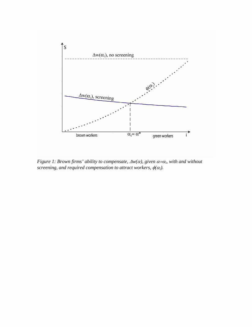
Figure 1: Brown firms’ ability to compensate, ∆w(α), given α=αi, with and without screening, and required compensation to attract workers, φ(αi).

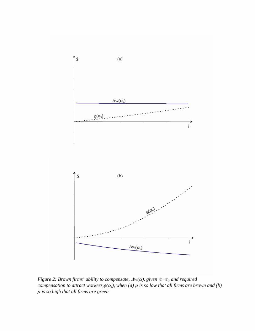
Figure 2: Brown firms’ ability to compensate, ∆w(α), given α=αi, and required compensation to attract workers,φ(αi), when (a) µ is so low that all firms are brown and (b) µ is so high that all firms are green.