Monte Carlo Simulation of correlated classical and …bonitz/si08/talks/August_6th/Morning... ·...
66
Monte Carlo Simulation of correlated classical and quantum plasmas Alexey Filinov Institut f¨ ur Theoretische Physik und Astrophysik, Christian-Albrechts-Universit¨ at zu Kiel, D-24098 Kiel, Germany Alexey Filinov Monte Carlo Simulation of correlated classical and quantum plasm Introduction: many-body methods in quantum mechanics Statistical physics: partition function, statistical weights, DM Path Integral MC as a stochastic method for thermodynamics Quantum statistics. PIMC for bosons and fermions Practical issues. Applications
Transcript of Monte Carlo Simulation of correlated classical and …bonitz/si08/talks/August_6th/Morning... ·...

Monte Carlo Simulation of correlated classical andquantum plasmas
Alexey Filinov
Institut fur Theoretische Physik und Astrophysik, Christian-Albrechts-Universitat zuKiel, D-24098 Kiel, Germany
August 6, 2008
Alexey Filinov Monte Carlo Simulation of correlated classical and quantum plasmas
Introduction: many-body methods in quantum mechanics
Statistical physics: partition function, statistical weights, DM
Path Integral MC as a stochastic method for thermodynamics
Quantum statistics. PIMC for bosons and fermions
Practical issues. Applications

Methods for many-body problems
Many-body Schrodinger equation
HΨ(R) = EΨ(R), H = −1
2
Xi
∇2i +
Xi
Vext(ri ) +Xi<j
1
|ri − rj |
We are interested in
energy spectrum: ground state, low-excited states
expectation values of operators 〈Ψn|A|Ψn〉/〈Ψn|Ψn〉Theoretical approaches (scaling with system size):
1 Direct diagonalization (CI) ∼ N6:– most exact method but only small systems
2 Mean field (DFT, HF) ∼ N3:– large system sizes, approximation on exchange/correlation
3 Quantum MC (VMC, DMC, GFMC, PIMC) ∼ N4:– calculations with full inclusion of many-body correlation effects, mostaccurate benchmark for medium-large systems
Alexey Filinov Monte Carlo Simulation of correlated classical and quantum plasmas

Direct diagonalization and mean-field solutions
Direct diagonalization:
Solve the matrix eigenvalue problem in a complete orthonormal basis set of wavefunctions (CI method)
ΨCI =KX
i=1
ci Φi ,
KXi=1
〈Φi |H|Φj〉cj = ECI
KXi=1
〈Φi |Φj〉cj
Alexey Filinov Monte Carlo Simulation of correlated classical and quantum plasmas

Direct diagonalization and mean-field solutions
Mean-field
Starting point – non-interacting Hartree-Fock wave functions.We introduce (Ψ1, . . . ,ΨN) – occupied orbitals and (ΨN+1, . . .) – virtual orbitals.
DHF (r1, . . . , rN) =
˛˛ Ψ1(r1) Ψ1(r2) . . . Ψ1(rN)
......
. . ....
ΨN(r1) ΨN(r2) . . . ΨN(rN)
˛˛
Spin orbitals: Ψi (r) = Φi (r)χSi (σ)Spatial part, Φi (r), satisfy HF-equations:"
−1
2∇2 + Vext(r) +
NXj=1
Zdr′|Φj(r
′)|2
|r − r′|
#Φi (r) +
hVHF Φi
i(r) = εi Φi (r)
Now we consider excitations to virtual orbitals: single, double, three, . . . -bodyexcitations
Ψ = c0 DHF + c1 D1 + c2 D2 + . . .
Goal: Construct more compact form of Ψ.
Alexey Filinov Monte Carlo Simulation of correlated classical and quantum plasmas

Variational Monte Carlo (VMC)
– Stochastic solution of Scrodinger equation.
Consider expectation values of the Hamiltonian on Ψ
Ev = 〈Ψ|H|Ψ〉/〈Ψ|Ψ〉 =
ZdR
HΨ(R)
Ψ(R)
!|Ψ(R)|2R
dR ′ |Ψ(R ′)|2=
=
ZdR EL(R) ρ(R) = 〈EL(R)〉ρ
where EL(R) is local energy and ρ(R) = A |Ψ(R)|2 is the distribution function,R = (r1, . . . , rN).Two main steps of VMC:
1 Sample R using ρ(R): random walk in the space of degrees of freedom
2 Average local energy
Ev = 〈EL(R)〉ρ =1
M
MXi=1
EL(Ri )± σE/√
M, σ2E = 〈(EL(R)− Ev )2〉ρ
Use zero-variance principle to find best estimation of a true wave function
Consider Ψ→ Ψ0, EL(R) =HΨ0(R)
Ψ0(R)= E0 = const | ⇒ σE → 0.
Alexey Filinov Monte Carlo Simulation of correlated classical and quantum plasmas

Variational Monte Carlo (continued)
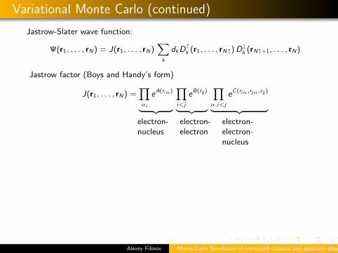
Jastrow-Slater wave function:
Ψ(r1, . . . , rN) = J(r1, . . . , rN)X
k
dkD↑k (r1, . . . , rN↑) D↓k (rN↑+1, . . . , rN)
Jastrow factor (Boys and Handy’s form)
J(r1, . . . , rN) =Yαi
eA(riα)
| z Yi<j
eB(rij )
| z Yα,i<j
eC(riα,rjα,rij )
| z where A,B,C are polynomials of scaled variables r = b r/(1 + αr) of the n-order
and recover most of the correlation energy Ecorr = Eexact − EHF .Practical notes:
Jastrow factors are optimized by variance/energy minimization
Orbitals and set of dk coefficients in determinantal part are obtained:– Hartree-Fock or DFT (LDA, GGA)– CI or multi-configuration self-consistent field calculations– Optimized by energy minimization
References: Foulkes et al., Rev.Mod.Phys. 73, 33 (2001);Filippi, Umrigar, J.Chem.Phys. 105, 213 (1996) and references therein.
Alexey Filinov Monte Carlo Simulation of correlated classical and quantum plasmas

Variational Monte Carlo (continued)
Jastrow-Slater wave function:
Ψ(r1, . . . , rN) = J(r1, . . . , rN)X
k
dkD↑k (r1, . . . , rN↑) D↓k (rN↑+1, . . . , rN)
Jastrow factor (Boys and Handy’s form)
J(r1, . . . , rN) =Yαi
eA(riα)
| z Yi<j
eB(rij )
| z Yα,i<j
eC(riα,rjα,rij )
| z where A,B,C are polynomials of scaled variables r = b r/(1 + αr) of the n-order
and recover most of the correlation energy Ecorr = Eexact − EHF .
Practical notes:
Jastrow factors are optimized by variance/energy minimization
Orbitals and set of dk coefficients in determinantal part are obtained:– Hartree-Fock or DFT (LDA, GGA)– CI or multi-configuration self-consistent field calculations– Optimized by energy minimization
References: Foulkes et al., Rev.Mod.Phys. 73, 33 (2001);Filippi, Umrigar, J.Chem.Phys. 105, 213 (1996) and references therein.
Alexey Filinov Monte Carlo Simulation of correlated classical and quantum plasmas
Variational Monte Carlo (continued)
Jastrow-Slater wave function:
Ψ(r1, . . . , rN) = J(r1, . . . , rN)X
k
dkD↑k (r1, . . . , rN↑) D↓k (rN↑+1, . . . , rN)
Jastrow factor (Boys and Handy’s form)
J(r1, . . . , rN) =Yαi
eA(riα)
| z Yi<j
eB(rij )
| z Yα,i<j
eC(riα,rjα,rij )
| z
where A,B,C are polynomials of scaled variables r = b r/(1 + αr) of the n-orderand recover most of the correlation energy Ecorr = Eexact − EHF .Practical notes:
Jastrow factors are optimized by variance/energy minimization
Orbitals and set of dk coefficients in determinantal part are obtained:– Hartree-Fock or DFT (LDA, GGA)– CI or multi-configuration self-consistent field calculations– Optimized by energy minimization
References: Foulkes et al., Rev.Mod.Phys. 73, 33 (2001);Filippi, Umrigar, J.Chem.Phys. 105, 213 (1996) and references therein.
Alexey Filinov Monte Carlo Simulation of correlated classical and quantum plasmas
electron-electron-nucleus
electron-electron
electron-nucleus

Variational Monte Carlo (continued)
Jastrow-Slater wave function:
Ψ(r1, . . . , rN) = J(r1, . . . , rN)X
k
dkD↑k (r1, . . . , rN↑) D↓k (rN↑+1, . . . , rN)
Jastrow factor (Boys and Handy’s form)
J(r1, . . . , rN) =Yαi
eA(riα)
| z Yi<j
eB(rij )
| z Yα,i<j
eC(riα,rjα,rij )
| z
where A,B,C are polynomials of scaled variables r = b r/(1 + αr) of the n-orderand recover most of the correlation energy Ecorr = Eexact − EHF .
Practical notes:
Jastrow factors are optimized by variance/energy minimization
Orbitals and set of dk coefficients in determinantal part are obtained:– Hartree-Fock or DFT (LDA, GGA)– CI or multi-configuration self-consistent field calculations– Optimized by energy minimization
References: Foulkes et al., Rev.Mod.Phys. 73, 33 (2001);Filippi, Umrigar, J.Chem.Phys. 105, 213 (1996) and references therein.
Alexey Filinov Monte Carlo Simulation of correlated classical and quantum plasmas
electron-electron-nucleus
electron-electron
electron-nucleus

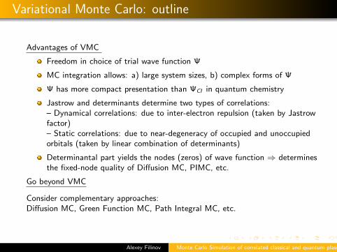
Variational Monte Carlo: outline
Advantages of VMC
Freedom in choice of trial wave function Ψ
MC integration allows: a) large system sizes, b) complex forms of Ψ
Ψ has more compact presentation than ΨCI in quantum chemistry
Jastrow and determinants determine two types of correlations:– Dynamical correlations: due to inter-electron repulsion (taken by Jastrowfactor)– Static correlations: due to near-degeneracy of occupied and unoccupiedorbitals (taken by linear combination of determinants)
Determinantal part yields the nodes (zeros) of wave function ⇒ determinesthe fixed-node quality of Diffusion MC, PIMC, etc.
Go beyond VMC
Alexey Filinov Monte Carlo Simulation of correlated classical and quantum plasmas

Variational Monte Carlo: outline
Advantages of VMC
Freedom in choice of trial wave function Ψ
MC integration allows: a) large system sizes, b) complex forms of Ψ
Ψ has more compact presentation than ΨCI in quantum chemistry
Jastrow and determinants determine two types of correlations:– Dynamical correlations: due to inter-electron repulsion (taken by Jastrowfactor)– Static correlations: due to near-degeneracy of occupied and unoccupiedorbitals (taken by linear combination of determinants)
Determinantal part yields the nodes (zeros) of wave function ⇒ determinesthe fixed-node quality of Diffusion MC, PIMC, etc.
Go beyond VMC
Dependence of the results on a trial wave function
No systematic procedure to construct analytical form of Ψ. One choses Ψbased on physical intuition
Easier to construct good Ψ for closed than for open shells.
The VMC wave function optimized for the energy is not necessary well suitedfor other quantities.
Alexey Filinov Monte Carlo Simulation of correlated classical and quantum plasmas
Variational Monte Carlo: outline
Advantages of VMC
Freedom in choice of trial wave function Ψ
MC integration allows: a) large system sizes, b) complex forms of Ψ
Ψ has more compact presentation than ΨCI in quantum chemistry
Jastrow and determinants determine two types of correlations:– Dynamical correlations: due to inter-electron repulsion (taken by Jastrowfactor)– Static correlations: due to near-degeneracy of occupied and unoccupiedorbitals (taken by linear combination of determinants)
Determinantal part yields the nodes (zeros) of wave function ⇒ determinesthe fixed-node quality of Diffusion MC, PIMC, etc.
Go beyond VMC
Consider complementary approaches:Diffusion MC, Green Function MC, Path Integral MC, etc.
Alexey Filinov Monte Carlo Simulation of correlated classical and quantum plasmas

Path Integral Monte Carlo: Applications
Path Integral Monte Carlo (PIMC) is an exact quantum-statistical method to getequilibrium properties.General description of the path integral formalism: Feynman (1972), Schulman(1981), Kleinert (1990).
Fermionic systems:
1 Dense hydrogen: Pierleoni et al. (1994), Magro et al. (1996), Militzer,Pollock (2000), V.Filinov, Bonitz, Ebeling et al. (2001)
2 Crystallization of one-component plasma: Jones, Ceperley (1996)
3 Electron-hole plasma: Shumway and Ceperley (1999)
4 Electrons in quantum dots: Egger, Hausler, Mac, Grabert (1999), Filinov,Bonitz, Lozovik (2001)
5 . . .
Alexey Filinov Monte Carlo Simulation of correlated classical and quantum plasmas

Path Integral Monte Carlo: Applications
Path Integral Monte Carlo (PIMC) is an exact quantum-statistical method to getequilibrium properties.General description of the path integral formalism: Feynman (1972), Schulman(1981), Kleinert (1990).
Bosonic systems:
1 Study of superfluid phase transition in 4He: Pollock and Ceperley(1984,1987)
2 Superfluidity in 4He clusters: Sindzingre et al. (1991)
3 Hard-sphere bosons: Gruter et al. (1996), Krauth, Holtzmann (1996)
4 Melting transition of molecular hydrogen surfaces: Wagner, Ceperley (1996)
5 Off-diagonal long-range order in solid 4He: Boninsegni, Prokof’ev, Svistunov(2006), Clark, Ceperley (2007)
6 . . .
Alexey Filinov Monte Carlo Simulation of correlated classical and quantum plasmas

Statistical Mechanics
Consider an average of observable A in canonical ensemble: fixed (N,V ,T ).
The probability that a system can be found in an energy eigenstate Ei isgiven by a Boltzmann factor (in thermal equilibrium)
A = 〈A〉(N,V , β) =
Pi e−Ei/kBT 〈i |A|i〉P
i e−Ei/kBT(1)
where 〈i |A|i〉 - expectation value in quantum state |i〉Direct way to proceed:→ Solve the Schrodinger equation for a many-body systems→ Calculate for each state with a non-negligible statistical weight e−Ei/kBT
matrix elements 〈i |A|i〉This approach is unrealistic !→ Even if we solve N-particle Schrodinger equation number of states which
contribute to the average would be astronomically large, e.g. 101025
!→ Direct numerical evaluation is unfeasible
We need another approach ! Equation (1) can be simplified in classical limit.
Alexey Filinov Monte Carlo Simulation of correlated classical and quantum plasmas

Statistical Mechanics: choice of basis
Idea:
1 Rewrite Eq. (1) in a from which does not depend on a specific basis
Z =X
i
e−Ei/kBT =X
i
〈i |e−βH |i〉 = Tr[e−βH ] =X
j
〈j |e−βH |j〉
where |j〉 is an arbitrary basis set, full and orthonormal.
2 Examples: eigenfunctions of momentum and position operators
pi |p〉 = pi |p〉, ri |r〉 = ri |r〉,
K |P〉 =
NX
i=1
pi
2mi
!|P〉 =
NX
i=1
pi
2mi
!|P〉
V |R〉 =“X
Vext (ri ) + Vij (ri , rj)”|R〉 =
“XVext(ri ) + Vij(ri , rj)
”|R〉
3 Both kinetic and potential operators are not diagonal in momentum or
coordinate representations, but separately e−βK , e−βV are
〈r |e−βK |r ′〉 =
Zdp′dp′′〈r |p′〉〈p′|e−β
Ppi/2mi |p′′〉〈p′′|r ′〉 =
NYi=1
λ−dND e
− π
λ2D
(ri−r′i )2
Alexey Filinov Monte Carlo Simulation of correlated classical and quantum plasmas

Statistical Mechanics: operator decomposition
Commutation relations. Baker-Campbell-Hausdorf formula:For any pair X , Y of non-commuting operators [X , Y ] = XY − YX 6= 0
eτ X eτ Y = eZ (2)
Z = τ(X +Y )+τ 2
2[X ,Y ]+
τ 3
12([X ,X ,Y ] + [Y ,Y ,X ])+
τ 4
24[X ,Y ,Y ,X ]+O(τ 5)
Consider now X = K , Y = V and τ = β/M 1 (M 1).General approach to factorize the exponent
eτ(K+V ) =nY
j=1
eajτK ebjτV + O(τ n+1)
Set of coeff. ai , bi are determined by required order of accuracy from Eq. (2).
Operator decomposition. Lower order factorization schemes
First order: eτ(K+V ) = eτK eτV eO(τ2)
Second order: eτ(K+V ) = e12τK eτV e
12τK eO(τ3)
Fourth order: eτ(K+V ) = e16τV e
12τK e
16τ V e
12τK e
16τV eO(τ5),
V = V +1
48τ 2[V , [K ,V ]] - correction to classical potential
Alexey Filinov Monte Carlo Simulation of correlated classical and quantum plasmas

Statistical Mechanics: classical partition function
We start from the simplest first order factorization applied at inverse
temperature β: e−β(K+V ) = e−βK e−βV eO(β2[K ,V ])
Using [K ,V ] ∼ ~ and considering quasi-classical limit ~→ 0 and hightemperatures β → 0 we can write
Trhe−βH
i≈
XR,P,R′,P′
〈R|e−βV |R ′〉〈R ′|P ′〉〈P ′|e−βK |P〉〈P|R〉 = ZNVT · Q idealNVT
→ Full partition function is written in terms of ideal gas partition functionQ ideal
NVT and configuration integral ZNVT .
Alexey Filinov Monte Carlo Simulation of correlated classical and quantum plasmas
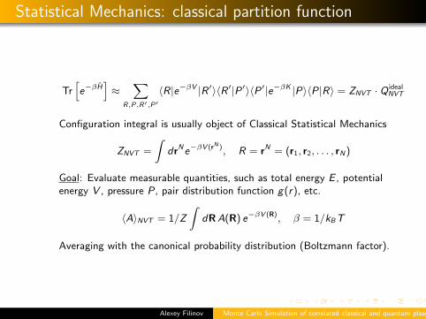
Statistical Mechanics: classical partition function
Trhe−βH
i≈
XR,P,R′,P′
〈R|e−βV |R ′〉〈R ′|P ′〉〈P ′|e−βK |P〉〈P|R〉 = ZNVT · Q idealNVT
Configuration integral is usually object of Classical Statistical Mechanics
ZNVT =
ZdrNe−βV (rN ), R = rN = (r1, r2, . . . , rN)
Goal: Evaluate measurable quantities, such as total energy E , potentialenergy V , pressure P, pair distribution function g(r), etc.
〈A〉NVT = 1/Z
ZdR A(R) e−βV (R), β = 1/kBT
Averaging with the canonical probability distribution (Boltzmann factor).
Alexey Filinov Monte Carlo Simulation of correlated classical and quantum plasmas

Statistical Mechanics: classical partition function
Trhe−βH
i≈
XR,P,R′,P′
〈R|e−βV |R ′〉〈R ′|P ′〉〈P ′|e−βK |P〉〈P|R〉 = ZNVT · Q idealNVT
The ideal gas part Q idealNVT still should be treated quantum mechanically.
Consider N particles in a box of volume V = L3
εk =~2k2
2m, k =
π
L(nxx + nyy + nzz),
∆nx =L
πdkx =
L
π~dpx ,
Xnx ,ny ,nz
→ L3
(π~)3
∞Z0
dp
Q idealNVT =
1
N!
„V
(2π~)3
Zdp e−βp2/2m
«N
=V N
N!λdND
, λ2D =
2π~2β
m
Alexey Filinov Monte Carlo Simulation of correlated classical and quantum plasmas
Statistical Mechanics: density matrix, paths integration
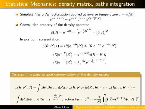
Simplest first order factorization applied at inverse temperature τ = β/M:
e−τ(K+V ) = e−τK e−τV eO(τ2[K ,V ])
Convolution property of the density operator
ρ(β) = e−βH =he−
βM
HiM
= [ρ(τ)]M
In position representation:
ρ(R,R ′; τ) = 〈R|e−τ H |R ′〉 ≈ 〈R|e−τK e−τV |R ′〉
〈R|e−τ V |R ′〉 = e−τV (R)δ(R − R ′),
〈R|e−τ T |R ′〉 = λ−3Nτ e
− πλ2
τ(R−R′)2
.
Discrete time path-integral representation of the density matrix
ρ(R,R ′;β) =
ZdR1dR2 . . .dRM−1 ρ(R,R1; τ)ρ(R1,R2; τ) · · · ρ(RM−1,R
′; τ) =
=
ZdR1dR2 . . .dRM−1 e
−MP
m=1Sm
, action term: Sm = − π
λ2τ
NYi=1
(rmi −rm−1
i )2+τV (rmi )
Alexey Filinov Monte Carlo Simulation of correlated classical and quantum plasmas

Thermodynamic Averages
Goal:
Obtain exact thermodynamic equilibrium configuration R = (r1, r2, . . . , rN) ofinteracting particles at given temperature T , particle number, N, externalfields etc.
Evaluate measurable quantities, such as total energy E , potential energy V ,pressure P, pair distribution function g(r), etc.
〈A〉(N, β) = 1/Z
ZdR A(R) e−βV (R), β = 1/kBT
Monte Carlo approach: approximate a continuous integral by a sum over set ofconfigurations xi sampled with the probability distribution p(x)Z
f (x) · p(x) dx ≈ 1
M
MXi=1
f (xi )p = 〈f (x)〉p
We need to sample with Boltzmann probability, pB(Ri ) = e−βV (Ri )/Z .
〈A〉 =1
M
Xi
A(Ri ) pB(Ri ) = 〈A(R)〉pB
⇒ Direct sampling with pB is not possible. Unknown normalization Z .
Alexey Filinov Monte Carlo Simulation of correlated classical and quantum plasmas

Thermodynamic Averages
Goal:
Obtain exact thermodynamic equilibrium configuration R = (r1, r2, . . . , rN) ofinteracting particles at given temperature T , particle number, N, externalfields etc.
Evaluate measurable quantities, such as total energy E , potential energy V ,pressure P, pair distribution function g(r), etc.
〈A〉(N, β) = 1/Z
ZdR A(R) e−βV (R), β = 1/kBT
Monte Carlo approach: approximate a continuous integral by a sum over set ofconfigurations xi sampled with the probability distribution p(x)Z
f (x) · p(x) dx ≈ 1
M
MXi=1
f (xi )p = 〈f (x)〉p
We need to sample with Boltzmann probability, pB(Ri ) = e−βV (Ri )/Z .Solution: Metropolis algorithm ⇒ lecture by Henning Baumgatner
Use Metropolis Monte Carlo procedure (Markov process) to sample allpossible configurations by moving individual particles.
Compute averages from fluctuating microstates.
Alexey Filinov Monte Carlo Simulation of correlated classical and quantum plasmas

Metropolis sampling method
Alexey Filinov Monte Carlo Simulation of correlated classical and quantum plasmas
Metropolis algorithm (1953)
1 Start from initial (random) configuration R0.
2 Using transition probability T (Ri → Ri+1) propose anew configuration: random displacement of one ormore particles.
3 Compute energy difference between two states:∆E = V (Ri+1)− V (Ri )
4 Consider two possibilities:
∆E ≤ 0 : always accept new configuration∆E > 0 : accept new configuration withprobability p = e−β∆E
5 Repeat steps (2)-(4) to obtain more and moreaccurate estimation: A = 〈A〉 ± δA with the error
estimation δA =
qτAσ
2A
M

Metropolis sampling method
⇒ Using Metropolis algorithm we sufficiently reduce a number sampledconfigurations to M ∼ 106 . . . 108.⇒ We account only configurations with non-vanishing weights: e−βV (Ri ).
Alexey Filinov Monte Carlo Simulation of correlated classical and quantum plasmas
Metropolis algorithm (1953)
1 Start from initial (random) configuration R0.
2 Using transition probability T (Ri → Ri+1) propose anew configuration: random displacement of one ormore particles.
3 Compute energy difference between two states:∆E = V (Ri+1)− V (Ri )
4 Consider two possibilities:
∆E ≤ 0 : always accept new configuration∆E > 0 : accept new configuration withprobability p = e−β∆E
5 Repeat steps (2)-(4) to obtain more and moreaccurate estimation: A = 〈A〉 ± δA with the error
estimation δA =
qτAσ
2A
M

Ergodicity
In simulations of classical systems we need to consider only configurationintegral
QclassNVT = Tr
he−βH
i=
1
N!
„2πmkBT
h2
«3N/2 ZdrN e−βV (rN )
The average over all possible microstates rN of a system is called ensembleaverage.
This can differ from real experiment: we perform a series of measurementsduring a certain time interval and then determine average of thesemeasurements.Example: Average particle density at spatial point r
ρ(r) = limt→∞1
t
tZ0
dt′ ρ(r, t′; rN(0), pN(0))
Alexey Filinov Monte Carlo Simulation of correlated classical and quantum plasmas

Ergodicity
System is ergodic: the time average does not depend on the initialconditions.→ We can perform additional average over many different initial conditions(rN(0), pN(0))
ρ(r) =1
N0
XN0
limt→∞1
t
tZ0
dt′ ρ(r, t′; rN(0), pN(0))
N0 is a number of initial conditions: same NVT , different rN(0), pN(0).
ρ(r) = 〈ρ(r)〉NVE time average = ensemble average
Nonergodic systems: glasses, metastable states, etc.
Alexey Filinov Monte Carlo Simulation of correlated classical and quantum plasmas

Quantum mechanical averages: distinguishable particles
Quantum mechanical average using N-particle wave function (pure ensemble)
〈A〉(N, β) = Tr [Aρ] = 1/Z
ZdR A(R)ψ∗(R)ψ(R)
Direct generalization to coherent superposition of N-particle wave functions
Finite temperatures (T > 0, mixed ensemble): use N-particle density matrixρ(r, r, β) instead of wave function
〈A〉(N, β) = 1/Z
ZdR A(R) ρ(R,R, β) =
= 1/Z
ZdRdR1 . . .dRM−1 A(R) ρ(R,R1; τ) . . . ρ(RM−1,R; τ) =
= 1/Z
ZdRdR1 . . .dRM−1 A(R) e
−MP
m=1Sm
Monte Carlo sampling is possible since diagonal density matrix is positive
P(R,R1, . . . ,RM−1) = e−
MPm=1
Sm
/Z = e−S(R)/Z = P(R) ≥ 0
Alexey Filinov Monte Carlo Simulation of correlated classical and quantum plasmas

Path Integral presentation
ρ(R,R ′;β) =
ZdR1dR2 . . .dRM−1 ρ(R,R1; τ)ρ(R1,R2; τ) · · · ρ(RM−1,R
′; τ) =
=
ZdR1dR2 . . .dRM−1 e
−MP
m=1Sm
, action term: Sm = − π
λ2τ
NYi=1
(rmi −rm−1
i )2+τV (rmi , r
mij )
Density matrix corresponds to a system of interacting polymers with classicalaction S :
“Spring” terms hold polymers (paths) together
Polymers interaction is specified by V (ri , rij)
Alexey Filinov Monte Carlo Simulation of correlated classical and quantum plasmas

Basic numerical issues of PIMC
1 How to sample the paths:it is necessary to explore the whole coordinate space for each intermediatepoint. This is very time consuming. To speed up convergence: move severalslices (points of path) at once.
2 How to construct more accurate actions:use effective interaction potentials which take into account two, three andhigher order correlation effects. More accurate actions help to reduce thenumber of time slices by a factor of 10 or more.
3 How to calculate physical properties:Expectation values of physical observables, e.g. energy, momentumdistribution, etc. can be calculated in different ways called estimators.Convergence can be improved by using an estimator with smaller statisticalvariance.
Alexey Filinov Monte Carlo Simulation of correlated classical and quantum plasmas

Trajectory sampling: local moves
For direct sampling of microstates distributed with
P(R) = e−S(R)/Z = e−
MPm=1
Sm
/Z
we need normalization factor Z - partition function.
Solution: use Metropolis algorithm to construct a sequence of microstateswith relative transition probabilities
T (Ri → Rf ) =P(Rf )
P(Ri )=
P(R ′,R ′1, . . . ,R′M−1)
P(R,R1, . . . ,RM−1)=
e−
MPm=1
S(R′m)
/Z
e−
MPm=1
S(Rm)
/Z
Probability of transition is defined by change in the actions of the final andinitial states
T (Ri → Rf ) = e−[S(Rf )−S(Ri )] = e−∆Skin−∆Sv
Alexey Filinov Monte Carlo Simulation of correlated classical and quantum plasmas

Trajectory sampling: local moves
Probability of transition is defined by change in the actions of the final andinitial states
T (Ri → Rf ) = e−[S(Rf )−S(Ri )] = e−∆Skin−∆Sv
Simple single slice path-sampling: move of rk → r′k involves segmentsrk−1, rk and rk−1, rk
∆Skin =π
λ2D(τ)
h(rk−1 − r′k)2 − (rk−1 − rk)2 + (r′k − rk+1)2 − (rk − rk+1)2
i,
∆Sv = τXi<j
ˆV (r′k(ij))− V (rk(ij))
˜Problem: local path sampling is stacked to a position of fixed end-points ⇒Exceedingly slow trajectory diffusion.
Alexey Filinov Monte Carlo Simulation of correlated classical and quantum plasmas
r′kr′krkrk

Trajectory sampling: multi-slice moves
Consider a general problem of constructing of a trajectory of a free particle(V = 0) connecting two end points r and r′.
Probability for a specific trajectory (product of free-particle imaginary-timepropagators)
T [Rn(r, r′, pτ)] =
p−1Ym=0
ρF (rm, rm+1, τ), ρF (rm, rm+1, τ) =1
λdτ
e−π(rm−rm+1)2/λ2τ
Normalization:PRn
T [Rn(r, r′, pτ)] =R
dr1 . . . drp−1T [Rn(r, r′, pτ)] = ρF (r, r′, pτ)
For sampling we use the normalized probability
T [Rn(r, r′, pτ)]
ρF (r, r′, pτ)=ρF (r, r1, τ)ρF (r1, r′, (p − 1)τ)
ρF (r, r′, pτ)· ρF (r1, r2, τ)ρF (r2, r′, (p − 2)τ)
ρF (r1, r′, (p − 1)τ)
× ρF (r2, r3, τ)ρF (r3, r′, (p − 3)τ)
ρF (r2, r′, (p − 2)τ). . .
ρF (rm−2, rm−1, τ)ρF (rm−1, r′, τ)
ρF (rm−2, r′, 2τ)
Each term in the product represents a normal (Gaussian) distribution aroundthe mid-point Rm and variance σm (m = 1, . . . , p − 1)
α =p −m
p −m + 1, Rm = αrm + (1− α)r′, σm =
rα
2πλτ
Alexey Filinov Monte Carlo Simulation of correlated classical and quantum plasmas

Trajectory sampling: multi-slice moves (continued)
T [Rn(x0, x6, 6τ)]
ρF (x0, x6, 6τ)=ρF (x0, x1, τ)ρF (x1, x6, 5τ)
ρF (x0, x6, 6τ)· ρF (x1, x2, τ)ρF (x2, x6, 4τ)
ρF (x1, x6, 5τ)
× ρF (x2, x3, τ)ρF (x3, x6, 3τ)
ρF (x2, x6, 4τ)· ρF (x3, x4, τ)ρF (x4, x6, 2τ)
ρF (x3, x6, 3τ)· ρF (x4, x5, τ)ρF (x5, x6, τ)
ρF (x4, x6, 2τ)
x0
x6
k = 1
x1
k = 2
x2
k = 3
x3
k = 4
x4
k = 5
x5
output
Alexey Filinov Monte Carlo Simulation of correlated classical and quantum plasmas

Construction of inter-particle exchange
1 Select a time interval along the imaginary time axis β.
2 Select at random a particle (e.g. shown by red trajectory).
3 Choose a second particle (green trajectory) from all neighbours N(i → f )within a distance of λD(4τ).
4 Sample new trajectories (rm+1i(j) , r
m+2i(j) , r
m+3i(j) ) using the free particles DM: ρF .
5 Determine number of neighbours for the reverse move N(f → i) and acceptor reject based on the change in potential action SV
A(i → f ) = min
»1,
N(f → i)
N(i → f )e−∆SV
–
Alexey Filinov Monte Carlo Simulation of correlated classical and quantum plasmas
4τ

Construction of inter-particle exchange
1 Select a time interval along the imaginary time axis β.
2 Select at random a particle (e.g. shown by red trajectory).
3 Choose a second particle (green trajectory) from all neighbours N(i → f )within a distance of λD(4τ). The exchange probability is proportional to
ρ(rmi , r
mj , P12r
m+4i , P12r
m+4j ) ∝ exp[−π(rm
i − rm+4j )2/λ2
D(4τ)]
4 Sample new trajectories (rm+1i(j) , r
m+2i(j) , r
m+3i(j) ) using the free particles DM: ρF .
5 Determine number of neighbours for the reverse move N(f → i) and acceptor reject based on the change in potential action SV
A(i → f ) = min
»1,
N(f → i)
N(i → f )e−∆SV
–
Alexey Filinov Monte Carlo Simulation of correlated classical and quantum plasmas
4τ

Construction of inter-particle exchange
1 Select a time interval along the imaginary time axis β.
2 Select at random a particle (e.g. shown by red trajectory).
3 Choose a second particle (green trajectory) from all neighbours N(i → f )within a distance of λD(4τ).
4 Sample new trajectories (rm+1i(j) , r
m+2i(j) , r
m+3i(j) ) using the free particles DM: ρF .
5 Determine number of neighbours for the reverse move N(f → i) and acceptor reject based on the change in potential action SV
A(i → f ) = min
»1,
N(f → i)
N(i → f )e−∆SV
–
Alexey Filinov Monte Carlo Simulation of correlated classical and quantum plasmas
4τ

Construction of inter-particle exchange
1 Select a time interval along the imaginary time axis β.
2 Select at random a particle (e.g. shown by red trajectory).
3 Choose a second particle (green trajectory) from all neighbours N(i → f )within a distance of λD(4τ).
4 Sample new trajectories (rm+1i(j) , r
m+2i(j) , r
m+3i(j) ) using the free particles DM: ρF .
5 Determine number of neighbours for the reverse move N(f → i) and acceptor reject based on the change in potential action SV
A(i → f ) = min
»1,
N(f → i)
N(i → f )e−∆SV
–Alexey Filinov Monte Carlo Simulation of correlated classical and quantum plasmas
4τ

Fermions/bosons: exchange operator
Alexey Filinov Monte Carlo Simulation of correlated classical and quantum plasmas
Any many-particle permutation state can be constructed by action of thepermutation operator P on the distinguishable density matrix:
Pρdist(r1, . . . rN, r1, . . . rN) =Yij
Pij ρdist(r1, . . . rN, r1, . . . rN)
Pij ρ(r1, . . . rN, . . . , ri , . . . , rj , . . .) = (±1) ρ(r1, . . . rN, . . . , rj , . . . , ri , . . .)
We can restore identical permutations bytwo successive pair-transpositions:
P34
»12345
12534
–→»
12345
12354
–,
P45
»12345
12354
–→»
12345
12345
–
Two identical permutations:ˆ
1212
˜.
One three particle permutation:ˆ
345534
˜.

Fermionic/bosonic density matrix
Due to the Fermi/Bose statistics the total density matrix should beantisymmetric/symmetric under arbitrary exchange of identical particles (e.g.electrons, holes, bosonic atoms). We replace ρ→ ρA/S for fermions/bosons.
Construct ρA/S as superposition of all N! permutations.Example: two types (e,h) of particles with particle numbers Ne and Nh
ρ(Re ,Rh,Re ,Rh;β) = (Ne !Nh!)−1XPe ,Ph
(−1)Pe (−1)Phρ(Re ,Rh, PeRe , PhRh;β)
Overall possible number of permutations: N = Ne ! · Nh!. Total densitymatrix is antisymmetric.
Illustration: 2 electrons and 2 holes. N = 2! · 2! permutations.
Alexey Filinov Monte Carlo Simulation of correlated classical and quantum plasmas

Cycle-length distribution: T -dependence
Alexey Filinov Monte Carlo Simulation of correlated classical and quantum plasmas
System: Fully spin polarized N electrons(or bosons) in 2D parabolic quantum dot.
Classical system: only identitypermutations.
Ideal/Interacting identical particles atT → 0: equal probability of allpermutations length L.
Ideal bosons: threshold value givescondensate fraction.

Cycle-length distribution: ideal Bose gas in traps
Cq – Number of permutation cycles with length q.
Partition function
ZN(β) =X Cq restr.
NYq=1
Z1(qβ)Cq
Cqq!qCq,
NXq=1
qCq = N
Number of particles occupying energy level Ei
〈Ni 〉 (β) =NX
q=1
e−qβEi
Z1(qβ)〈qCq〉
Mean energy
〈E〉 (β) =NX
q=1
E1(qβ) 〈qCq〉
Quantum mechanical moment of inertia. Superfluid fraction in a trappedsystem
Iqm = β 〈L2z〉 = 2~2
NXq=1
qβe−qβ~ω⊥
(1− e−qβ~ω⊥)2〈qCq〉
γs = 1− Iqm
IclassAlexey Filinov Monte Carlo Simulation of correlated classical and quantum plasmas

BEC/Superfluidity in macroscopic systems
In Path Integral presentation presence of the off-diagonal long-range order andsuperfluidity is related to the winding number: number of times the long cycleswind around simulation box.
Alexey Filinov Monte Carlo Simulation of correlated classical and quantum plasmas
ODLRO in solid 4He:
N. Prokof’ev, B. Svistunov, M. Boninsegni, PRE 74, 036701
(2007)
−10−10
−5
−5
0
0
5
5
10
10
n(r, r′)|r−r′|→∞ → N0
BEC: non-vanishing one-particle density ma-trix at large distances
n(r, r′) = N0φ∗0 (r)φ0(r′) +
Xi 6=0
niφ∗i (r)φi (r
′)Superfluid fraction:
γsf =ρs
ρ=
m〈W 2z 〉
2~2βρ
NXi=1
(rPi−r) = WL

Phase transition: normal solid-superfluid gas
Alexey Filinov Monte Carlo Simulation of correlated classical and quantum plasmas
rs = 32.9
rs = 33.4
rs = 34
N = 60bosonic excitons.Material: ZnSe.Effective dipole moment:
d = 6.6aB(ZnSe).
(realized by Ez = 20 kV/cmin 30 nm QW).Mass-asymmetry:
mh/me = 2.46
rs > 33.4→ Exciton crystal. Localexchanges of 2-7 atoms.
rs ≈ 33→ Crystal melting. Globalmacroscopic exchanges.

Phase transition: solid-superfluid gas (continued)
Structual transition is described byLindemann parameters: ur = 〈δr 2〉/a2
Simulation parameters:Number of excitons: N = 60 and 90Temperature: T = 3 · 10−4HaEffective exciton mass: mx = 3.46me
Dipole moment: d = 6.6aB
Critical density of solid-superfluid gastransition and onset of superfluidity:
ρ∗a2B ≈ 0.0033
Estimations for typical semiconductors:
(ZnSe-based QW)ρ∗ ≈ 3.5 · 109cm−2, T = 0.203K(GaAs-based QW)ρ∗ ≈ 3.74 · 1010cm−2, T = 0.044K
Alexey Filinov Monte Carlo Simulation of correlated classical and quantum plasmas

Fermion sign problem. Concepts of fermionic PIMC (1)
Metropolis algorithm gives the same distribution of permutations for bothFermi and Bose systems. The reason is that for sampling permutations weuse the modulus of the off-diagonal density matrix.
ρS/A(R,R;β) =1
N!
XP
(±1)Pρ(R, PR;β) =
=1
N!
XP
(±1)P
ZdR1 . . .dRM−1 ρ(R,R1;β) . . . ρ(RM−1, PR;β)
Bosons: all permutations contribute with the same (positive) sign
Fermions: positive and negative terms (corresponding to even and oddpermutations) are close in their absolute value and cancel each other.
Accurate calculation of this small difference is drastically hampered with theincrease of quantum degeneracy (low T, high density).
Alexey Filinov Monte Carlo Simulation of correlated classical and quantum plasmas

How to overcome fermion problem in Quantum MC
Universal solution is not known !!!
Alexey Filinov Monte Carlo Simulation of correlated classical and quantum plasmas
How to overcome fermion problem in Quantum MC
1 Fixed-node (fixed-phase) approximation
Use restricted (reduced) area of PIMC integration which contains only evenpermutations. Most of the area with the cancellation of even and oddpermutations are excluded using an approximate trial ansatz for theN-particle fermion density matrix. Requires knowledge of nodes of DM.
References: D.M.Ceperley, Fermion Nodes, J. Stat. Phys. 63, 1237 (1991);D.M.Ceperley, Path Integral Calculations of Normal Liquid 3He, Phys. Rev.Lett. 69, 331 (1992).
Alexey Filinov Monte Carlo Simulation of correlated classical and quantum plasmas

How to overcome fermion problem in Quantum MC
2 Direct PIMC
Do not sample individual permutations in the sum. Instead use the fullexpression presented in a form of an determinant. In this case the absolutevalue of the determinant is used in the sampling probabilities. Its valuebecomes close to zero in the regions of equal contributions of even and oddpermutations and Monte Carlo sampling successfully avoids such regions.
References: V.S.Filinov, M.Bonitz, W.Ebeling, and V.E.Fortov,Thermodynamics of hot dense H-plasmas: Path integral Monte Carlosimulations and analytical approximations, Plasma Physics and ControlledFusion 43, 743 (2001).
Alexey Filinov Monte Carlo Simulation of correlated classical and quantum plasmas

How to overcome fermion problem in Quantum MC
3 Multilevel-blocking PIMC
Trace the cancellations of permutations by grouping the path coordinatesinto blocks (levels). Use numerical integration to get good estimation of thefermion density matrix at lower temperature. Further use it in the samplingprobabilities of path coordinates on the next level (corresponding to thedensity matrix at even lower temperature). Most of the sign fluctuations arealready excluded at higher levels and sampling at low levels (lowertemperatures) becomes more efficient.
References: R.Egger, W.Hausler, C.H.Mak, and H.Grabert, Crossover fromFermi Liquid to Wigner Molecule Behavior in Quantum Dots, Phys. Rev.Lett. 82, 3320 (1999).
Alexey Filinov Monte Carlo Simulation of correlated classical and quantum plasmas
Why go behond Canonical ensemble
Alexey Filinov Monte Carlo Simulation of correlated classical and quantum plasmas
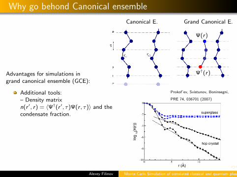
Advantages for simulations ingrand canonical ensemble (GCE):
Additional tools:– Density matrixn(r ′, r) = 〈Ψ†(r ′, τ)Ψ(r , τ)〉 and thecondensate fraction.
– µ is an input parameter, and 〈N〉µ is asimple diagonal property.– Compressibility, kVT = 〈(N − 〈N〉)2〉µ .Solve ergodicity issue for disorder problems
Allows for efficient sampling ofexponentially rare event
Prokof’ev, Svistunov, Boninsegni,
PRE 74, 036701 (2007)
Grand Canonical E.Canonical E.
Ψ(r)
Ψ†(r)

Why go behond Canonical ensemble
Alexey Filinov Monte Carlo Simulation of correlated classical and quantum plasmas
Advantages for simulations ingrand canonical ensemble (GCE):
Additional tools:– Density matrixn(r ′, r) = 〈Ψ†(r ′, τ)Ψ(r , τ)〉 and thecondensate fraction.– µ is an input parameter, and 〈N〉µ is asimple diagonal property.– Compressibility, kVT = 〈(N − 〈N〉)2〉µ .
Solve ergodicity issue for disorder problems
Allows for efficient sampling ofexponentially rare event
Grand Canonical E.Canonical E.
Ψ(r)
Ψ†(r)
5
10
15
20
25
30
35
40
45
50
55
60
0 20 40 60 80 100
Ave
rage
par
ticle
num
ber
N
Chemical potential µ in K
Average particle number for chemical potential (T=0.5 K)
100 200 300 400 500 600 700 800 900 1000 5
10
15
20
25
30
35
40
45
50
55
60
λ0.50.60.70.80.91.0
µ
〈N〉µ

Why go behond Canonical ensemble
Alexey Filinov Monte Carlo Simulation of correlated classical and quantum plasmas
Advantages for simulations ingrand canonical ensemble (GCE):
Additional tools:– Density matrixn(r ′, r) = 〈Ψ†(r ′, τ)Ψ(r , τ)〉 and thecondensate fraction.– µ is an input parameter, and 〈N〉µ is asimple diagonal property.– Compressibility, kVT = 〈(N − 〈N〉)2〉µ .Solve ergodicity issue for disorder problems
Allows for efficient sampling ofexponentially rare event
e−2R
p(x)dx

Improved high-temperature action
We need to improve the simple factorization formula for unbound potentials,e.g. V (r) = −1/r
ρ(R,R′, τ) ≈NY
i=1
ρF (ri , r′i , τ) · exp
24−τYj<k
u(rjk)
35⇒ Sampling is not possible as the DM can not be normalized.
Take into account two-body correlations “exactly”
ρ(R,R′; τ) ≈NY
i=1
ρF (ri , r′i ; τ)×Yj<k
ρ[2](rj , rk , r′j , r′k ; τ)
ρF (ri , r′i ; τ)ρF (rk , r′k ; τ)+ O(ρ[3]),
Three-body and higher order terms become negligible by decreasingτ = β/M.
Two-body density matrix ρ[2] can be obtained by solving two-particleproblem.
Replace singular potentials with finite effective potentials defined as
ρ(r, r′;β) = ρF (r, r′;β) expˆ−βU(r, r′;β)
˜Alexey Filinov Monte Carlo Simulation of correlated classical and quantum plasmas

Methods to obtain two-body density matrix
Sum over eigenstates of the Hamiltonian
ρ(r, r′, τ) =X
i
e−τEi Ψ∗i (r) Ψi (r′)
Can be used if all eigenstates are known analytically, e.g. for Coulombpotential (Pollock Comm. Phys. 52, 49 (1988)).
Feynman-Kac formula
ρ(r, r′;β) =
Z r(β)=r′
r(0)=r
Dr(τ) exp
24− βZ0
“mr2(τ)/2 + u12(r(τ)) dτ
”35 =˙e−u12
¸ρF
The average from e−u12 = exp
"−
βR0
u12(r(τ)) dτ
#can be calculated by a
Monte Carlo procedure by sampling all Gaussian random walks from r to r′.
Alexey Filinov Monte Carlo Simulation of correlated classical and quantum plasmas

Methods to obtain two-body density matrix
Matrix squaring technique (Klemm and Storer, 1974).Expansion in partial waves
ρ2D(r, r′;β) =1
2π√
r r ′
+∞Xl=−∞
ρl(r , r ′;β)e i lΘ,
ρ3D(r, r′;β) =1
4πr r ′
+∞Xl=0
(2l + 1) ρl(r , r ′;β) Pl(cos Θ)
Convolution equation for DM Semi-classical approximation: to start thematrix-squaring iterations
Perturbative: Kelbg, Ebeling, Deutsch, Feynman, Kleinert (1963-1995)
Φ (rij , β) =qi qj
rij
241− e−
r2ij
λ2ij +√π
rijλijγij
„1− erf
»γij
rijλij
–«35 .
Alexey Filinov Monte Carlo Simulation of correlated classical and quantum plasmas

Effective pair potential
Two-body effective pair potential: U(r, r′;β) = − 1β
ln [ρ(r, r′;β)/ρF (r, r′;β)] .
(a): Diagonal effective electron-proton potential (in units of Ha) for several cases:the DKP Φ0(r;β), the improved DKP Φ(r;β), variational potential W Ω,xm
1 , pairpotential Up corresponding to the “exact” density matrix. Each potential is givenat at three temperature values: 5 000, 40 000, 125 000 and 320 000 K. (b): thefunction U(β) + β∂U(β)/∂β for the same approximations and temperatures.
Alexey Filinov Monte Carlo Simulation of correlated classical and quantum plasmas
0 2 4 6-2.5
-2.0
-1.5
-1.0
-0.5
0.0
0 2 4 6
-1.5
-1.0
-0.5
0.0
Upair
ΦKelbg
W ω, xm
Φ0
Kelbg
320 000 K
125 000 K
40 000 K
r/aB
5 000 K
U(β)a)
Upair
ΦKelbg
W ω, xm
Φ0
Kelbg
r/aB
320 000 K
125 000 K
40 000 K 5 000 K
U(β)+β∆U(β)/∆βb)

Estimators for thermodynamic averages
Quantities of interest: energy, pressure (equation of state), specific heat, structurefactor, pair distribution functions, condensate or superfluid fraction, etc.
All quantities can be obtained by averaging with the thermal density matrix or asderivatives of partition function Z.
1 We usually calculate only ratios of integrals. Free energy and entropy requirespecial techniques.
E = − ∂
∂β(lnZ) = − 1
Z
∂Z
∂β= − 1
Z
ZdR
∂ρ(R,R;β)
∂β.
2 The variance of some estimators can be large: 〈A〉 = 1M
MPi=1
A(Ri )±σA/√
M
3 Many quantities are defined as dynamical quantities, but we are limited toonly imaginary time (static properties) or linear response results.
Alexey Filinov Monte Carlo Simulation of correlated classical and quantum plasmas

Estimators for thermodynamic averages
Quantities of interest: energy, pressure (equation of state), specific heat, structurefactor, pair distribution functions, condensate or superfluid fraction, etc.
All quantities can be obtained by averaging with the thermal density matrix or asderivatives of partition function Z.
1 We usually calculate only ratios of integrals. Free energy and entropy requirespecial techniques.
E = − ∂
∂β(lnZ) = − 1
Z
∂Z
∂β= − 1
Z
ZdR
∂ρ(R,R;β)
∂β.
2 The variance of some estimators can be large: 〈A〉 = 1M
MPi=1
A(Ri )± σA/√
M
E =dMN
2β−
*M−1Xi=0
Mm
2~2β2(Ri − Ri+1)2
+ρ(R;β)
+
*1
M
M−1Xi=0
V (Ri )
+ρ(R;β)
.
3 Many quantities are defined as dynamical quantities, but we are limited toonly imaginary time (static properties) or linear response results.
Alexey Filinov Monte Carlo Simulation of correlated classical and quantum plasmas

Estimators for thermodynamic averages
Quantities of interest: energy, pressure (equation of state), specific heat, structurefactor, pair distribution functions, condensate or superfluid fraction, etc.
All quantities can be obtained by averaging with the thermal density matrix or asderivatives of partition function Z.
1 We usually calculate only ratios of integrals. Free energy and entropy requirespecial techniques.
E = − ∂
∂β(lnZ) = − 1
Z
∂Z
∂β= − 1
Z
ZdR
∂ρ(R,R;β)
∂β.
2 The variance of some estimators can be large: 〈A〉 = 1M
MPi=1
A(Ri )± σA/√
M
Use virial estimators, e.g. Ri = R0 + λ∆
iPm=1
ξm, i = 1, . . . ,M − 1.
E =dN
2β+
fiV (R) + β
∂V (R)
∂R
∂R
∂β
flρ(R;β)
.
3 Many quantities are defined as dynamical quantities, but we are limited toonly imaginary time (static properties) or linear response results.
Alexey Filinov Monte Carlo Simulation of correlated classical and quantum plasmas
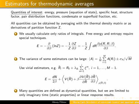
Estimators for thermodynamic averages
Quantities of interest: energy, pressure (equation of state), specific heat, structurefactor, pair distribution functions, condensate or superfluid fraction, etc.
All quantities can be obtained by averaging with the thermal density matrix or asderivatives of partition function Z.
1 We usually calculate only ratios of integrals. Free energy and entropy requirespecial techniques.
E = − ∂
∂β(lnZ) = − 1
Z
∂Z
∂β= − 1
Z
ZdR
∂ρ(R,R;β)
∂β.
2 The variance of some estimators can be large: 〈A〉 = 1M
MPi=1
A(Ri )± σA/√
M
Use virial estimators, e.g. Ri = R0 + λ∆
iPm=1
ξm, i = 1, . . . ,M − 1.
E =dN
2β+
fiV (R) + β
∂V (R)
∂R
∂R
∂β
flρ(R;β)
.
3 Many quantities are defined as dynamical quantities, but we are limited toonly imaginary time (static properties) or linear response results.
Alexey Filinov Monte Carlo Simulation of correlated classical and quantum plasmas

Discussion
Quantum and classical Monte Carlo methods are actively developingcomputational tools for exact treatment of many-body systems in equilibrium. Inthis lecture we give an introduction to path integral Monte Carlo simulations.
Almost exact method for thermodynamics of quantum systems at anyinteraction strength.
There are many technical and simulation details covers in recent reviewpapers.
Problems remain to be solved:– Fermion sign problem– Limitations to several hundred particles due to large computationaldemands– Efficient simulations of spin and magnetic effects
Alexey Filinov Monte Carlo Simulation of correlated classical and quantum plasmas