Monte Carlo Path Tracing - cs.princeton.edu · Monte Carlo Path Tracing COS 526, Fall 2016 Tom...
64
Monte Carlo Path Tracing COS 526, Fall 2016 Tom Funkhouser Slides from Rusinkiewicz , Shirley
Transcript of Monte Carlo Path Tracing - cs.princeton.edu · Monte Carlo Path Tracing COS 526, Fall 2016 Tom...
Monte Carlo Path Tracing
COS 526, Fall 2016
Tom Funkhouser
Slides from Rusinkiewicz, Shirley
Outline
• Motivation
• Monte Carlo integration
• Variance reduction techniques
• Monte Carlo path tracing
• Sampling techniques
• Conclusion
Motivation
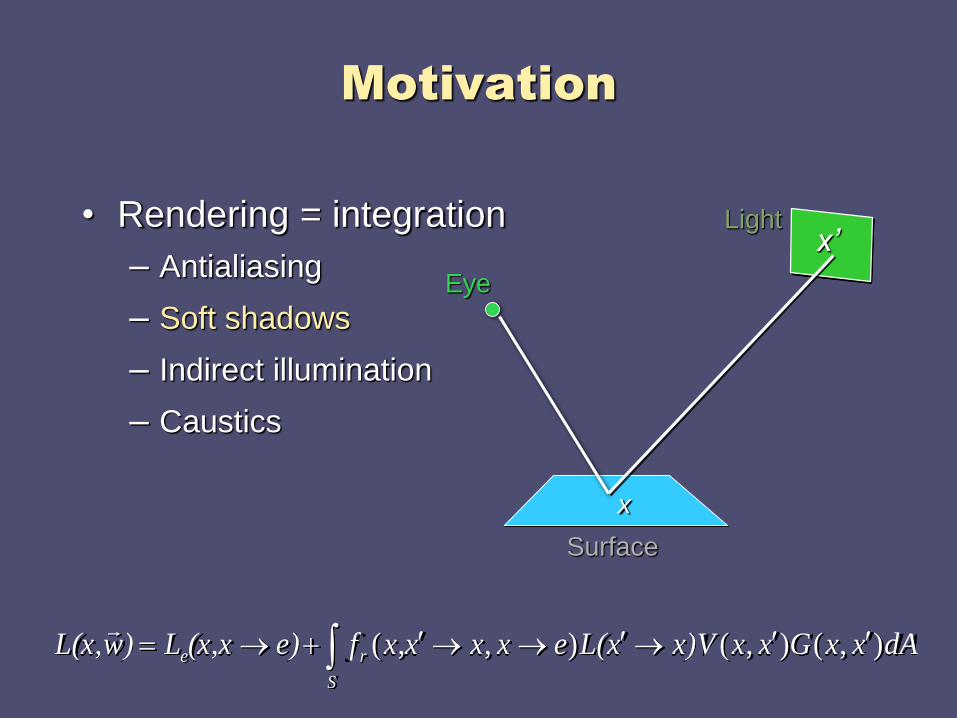
• Rendering = integration
– Antialiasing
– Soft shadows
– Indirect illumination
– Caustics

Motivation
• Rendering = integration
– Antialiasing
– Soft shadows
– Indirect illumination
– Caustics
Surface
Eye
Pixel
x
dAe)L(xLS
P
Motivation
• Rendering = integration
– Antialiasing
– Soft shadows
– Indirect illumination
– Caustics
Surface
Eye
Light
x
x’
dAxxGxxx)VxL(exxxxfe)(x,xL)wL(x,S
re ),(),(),,(
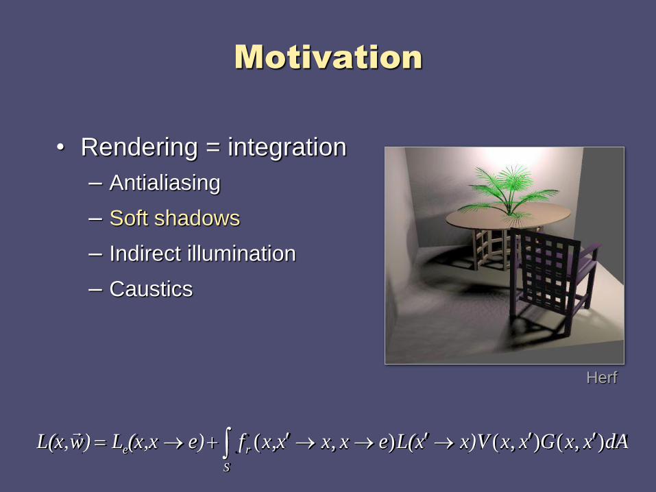
Motivation
• Rendering = integration
– Antialiasing
– Soft shadows
– Indirect illumination
– Caustics
Herf
dAxxGxxx)VxL(exxxxfe)(x,xL)wL(x,S
re ),(),(),,(
Motivation
• Rendering = integration
– Antialiasing
– Soft shadows
– Indirect illumination
– Caustics
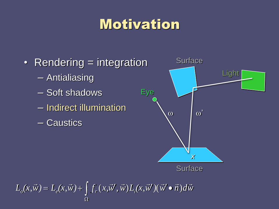
wdnw)w(x,Lwwxf)w(x,L)w(x,L ireo
)(),,(
Surface
Eye
Light
x
w
Surface
w’
Motivation
• Rendering = integration
– Antialiasing
– Soft shadows
– Indirect illumination
– Caustics
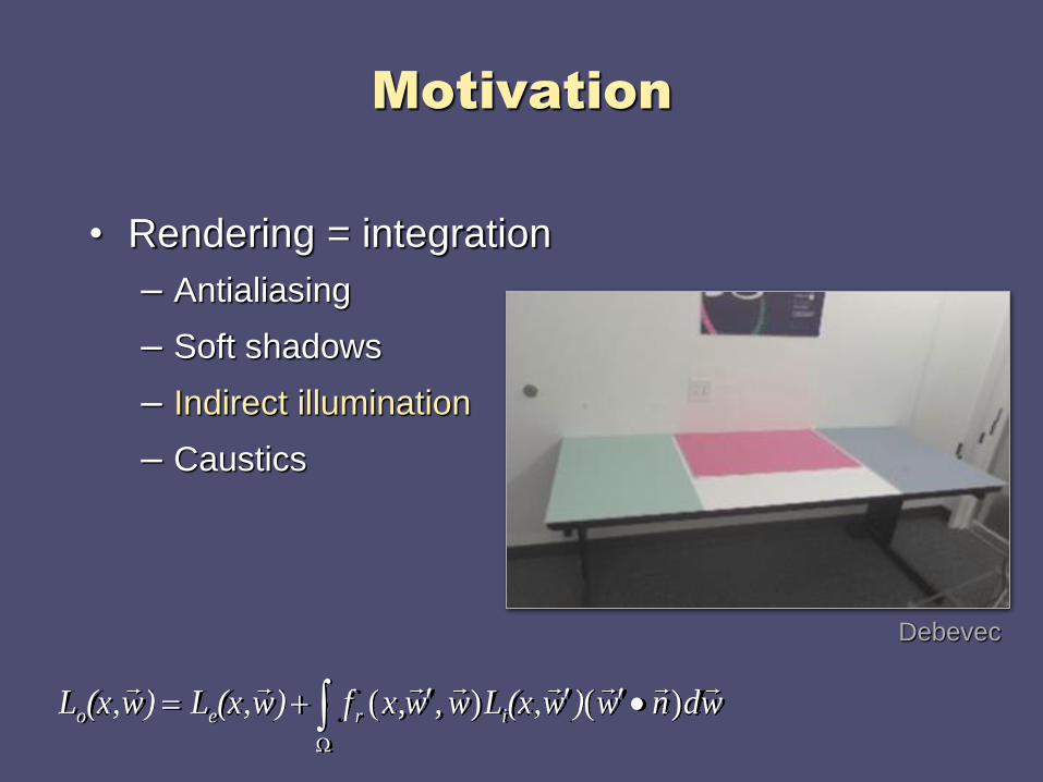
Debevec
wdnw)w(x,Lwwxf)w(x,L)w(x,L ireo
)(),,(
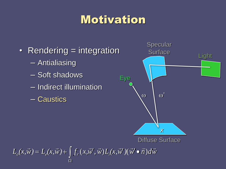
Motivation
• Rendering = integration
– Antialiasing
– Soft shadows
– Indirect illumination
– Caustics
Diffuse Surface
Eye
Light
x
w
Specular
Surface
w’
wdnw)w(x,Lwwxf)w(x,L)w(x,L ireo
)(),,(

Motivation
• Rendering = integration
– Antialiasing
– Soft shadows
– Indirect illumination
– Caustics
Jensen
wdnw)w(x,Lwwxf)w(x,L)w(x,L ireo
)(),,(
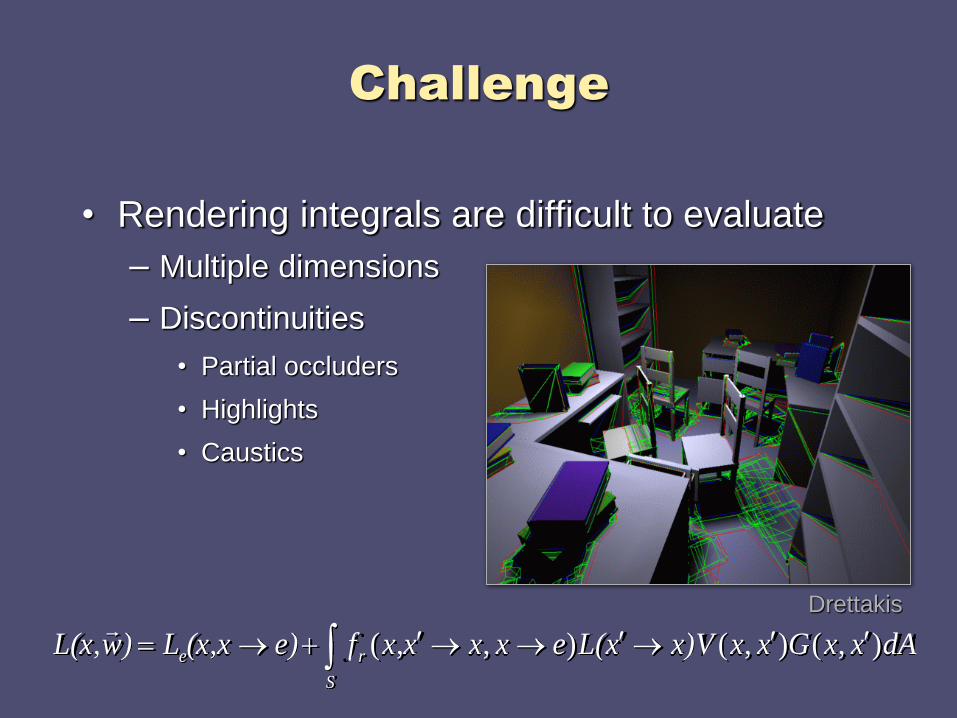
Challenge
• Rendering integrals are difficult to evaluate
– Multiple dimensions
– Discontinuities
• Partial occluders
• Highlights
• Caustics
Drettakis
dAxxGxxx)VxL(exxxxfe)(x,xL)wL(x,S
re ),(),(),,(

Challenge
• Rendering integrals are difficult to evaluate
– Multiple dimensions
– Discontinuities
• Partial occluders
• Highlights
• Caustics
Jensen
dAxxGxxx)VxL(exxxxfe)(x,xL)wL(x,S
re ),(),(),,(
Outline
• Motivation
• Monte Carlo integration
• Variance reduction techniques
• Monte Carlo path tracing
• Sampling techniques
• Conclusion
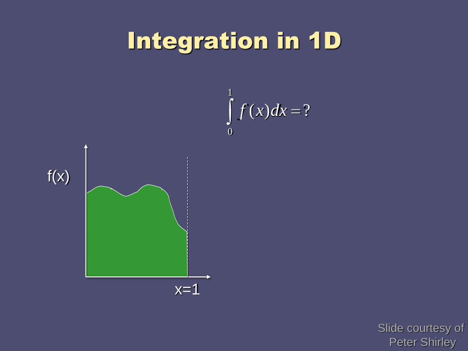
Integration in 1D
x=1
f(x)
?)(
1
0
dxxf
Slide courtesy of
Peter Shirley

We can approximate
x=1
f(x)g(x)
1
0
1
0
)()( dxxgdxxf
Slide courtesy of
Peter Shirley

Or we can average
x=1
f(x)
E(f(x))
))(()(
1
0
xfEdxxf
Slide courtesy of
Peter Shirley
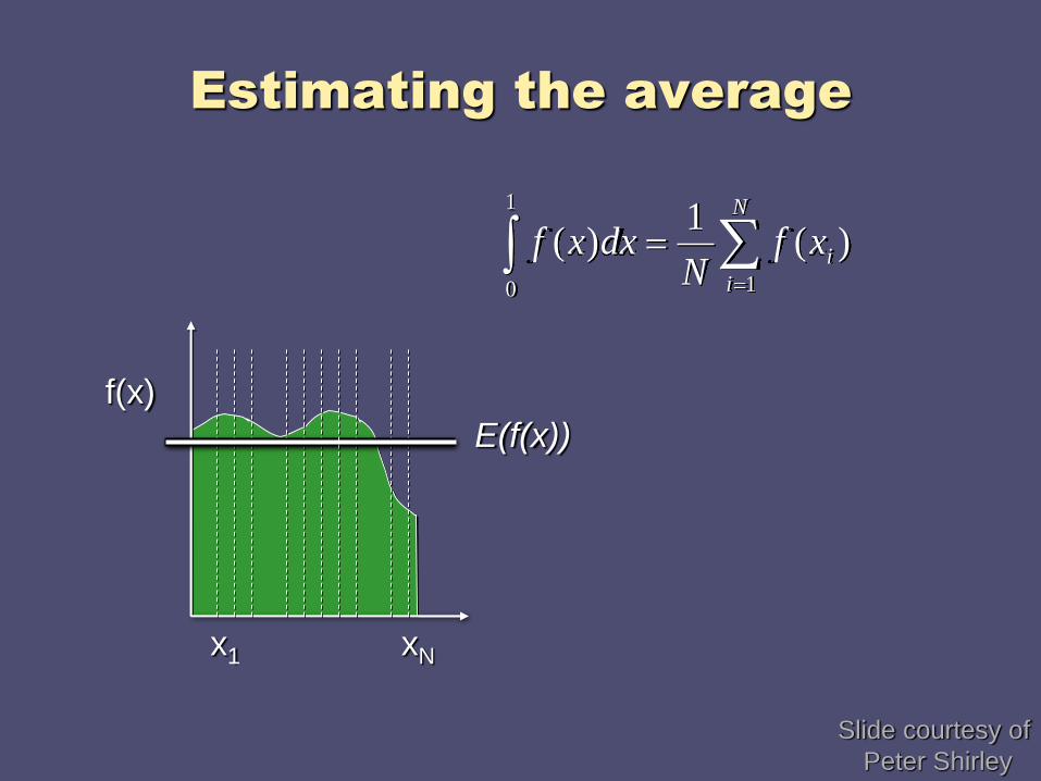
Estimating the average
x1
f(x)
xN
N
i
ixfN
dxxf1
1
0
)(1
)(
E(f(x))
Slide courtesy of
Peter Shirley
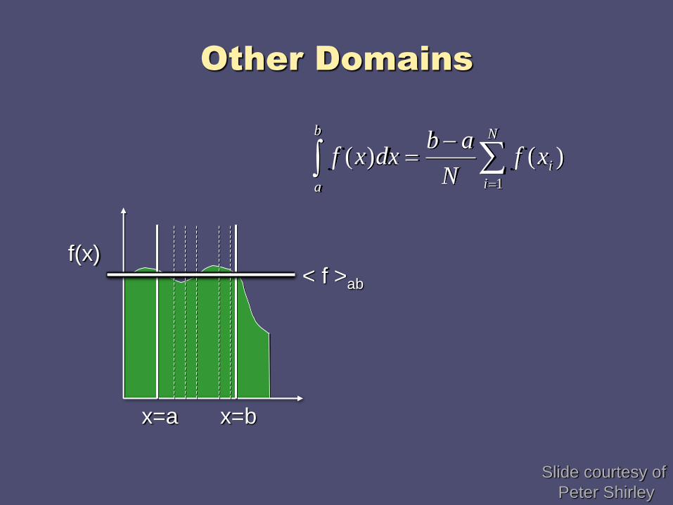
Other Domains
x=b
f(x)< f >ab
x=a
N
i
i
b
a
xfN
abdxxf
1
)()(
Slide courtesy of
Peter Shirley
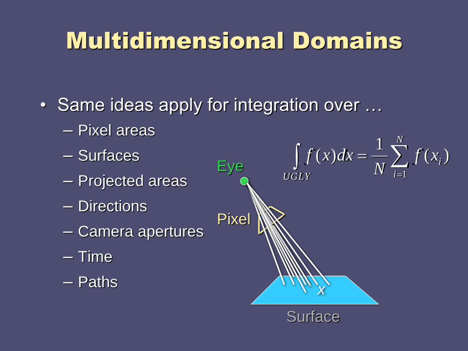
Multidimensional Domains
• Same ideas apply for integration over …
– Pixel areas
– Surfaces
– Projected areas
– Directions
– Camera apertures
– Time
– Paths
N
i
i
UGLY
xfN
dxxf1
)(1
)(
Surface
Eye
Pixel
x

Efficiency?
x1 xN
E(f(x))
2
1
))](()([1
)( xfExfN
xfVarN
i
i
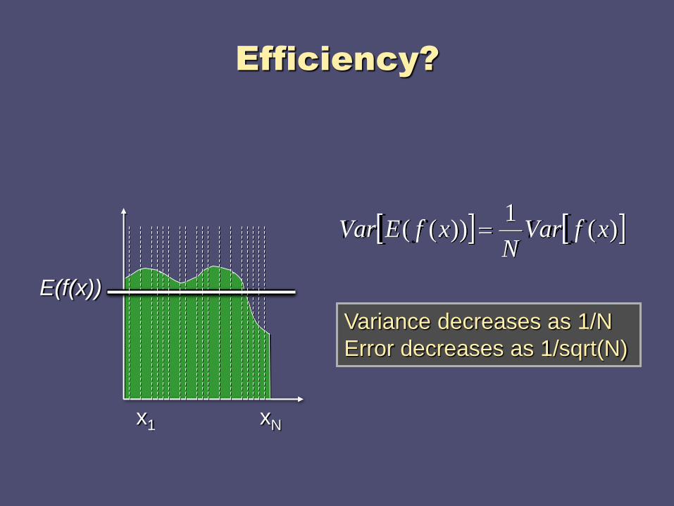
Efficiency?
x1 xN
E(f(x))
)(1
))(( xfVarN
xfEVar
Variance decreases as 1/N
Error decreases as 1/sqrt(N)
Outline
• Motivation
• Monte Carlo integration
• Variance reduction techniques
• Monte Carlo path tracing
• Sampling techniques
• Conclusion
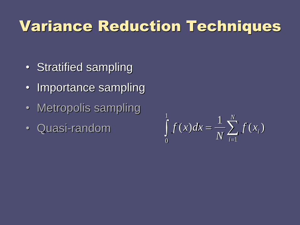
Variance Reduction Techniques
• Stratified sampling
• Importance sampling
• Metropolis sampling
• Quasi-random
N
i
ixfN
dxxf1
1
0
)(1
)(

Stratified Sampling
• Estimate subdomains separately
x1 xN
Ek(f(x))
Arvo
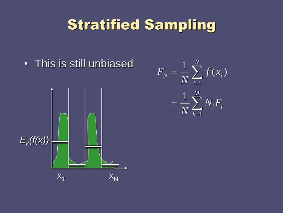
Stratified Sampling
• This is still unbiased
M
k
ii
N
i
iN
FNN
xfN
F
1
1
1
)(1
x1 xN
Ek(f(x))
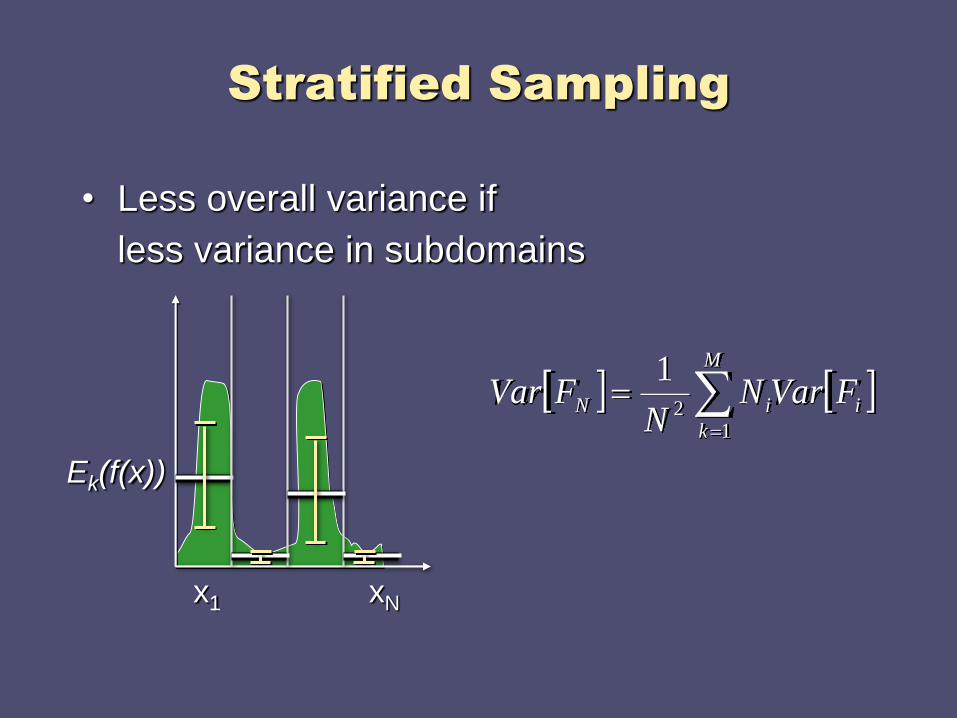
Stratified Sampling
• Less overall variance if
less variance in subdomains
M
k
iiN FVarNN
FVar1
2
1
x1 xN
Ek(f(x))

Variance Reduction Techniques
• Stratified sampling
• Importance sampling
• Metropolis sampling
• Quasi-random
N
i
ixfN
dxxf1
1
0
)(1
)(
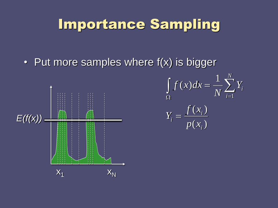
Importance Sampling
• Put more samples where f(x) is bigger
)(
)(
1)(
1
i
ii
N
i
i
xp
xfY
YN
dxxf
x1 xN
E(f(x))
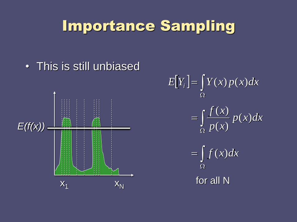
Importance Sampling
• This is still unbiased
x1 xN
E(f(x))
dxxf
dxxpxp
xf
dxxpxYYE i
)(
)()(
)(
)()(
for all N
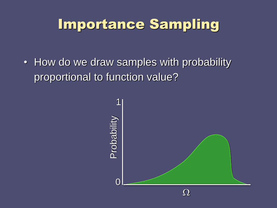
Importance Sampling
• How do we draw samples with probability
proportional to function value?
Pro
babili
ty
0
1
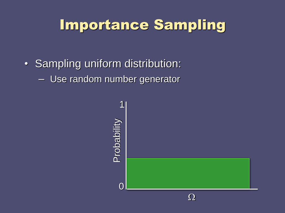
Importance Sampling
• Sampling uniform distribution:
– Use random number generator
Pro
babili
ty
0
1
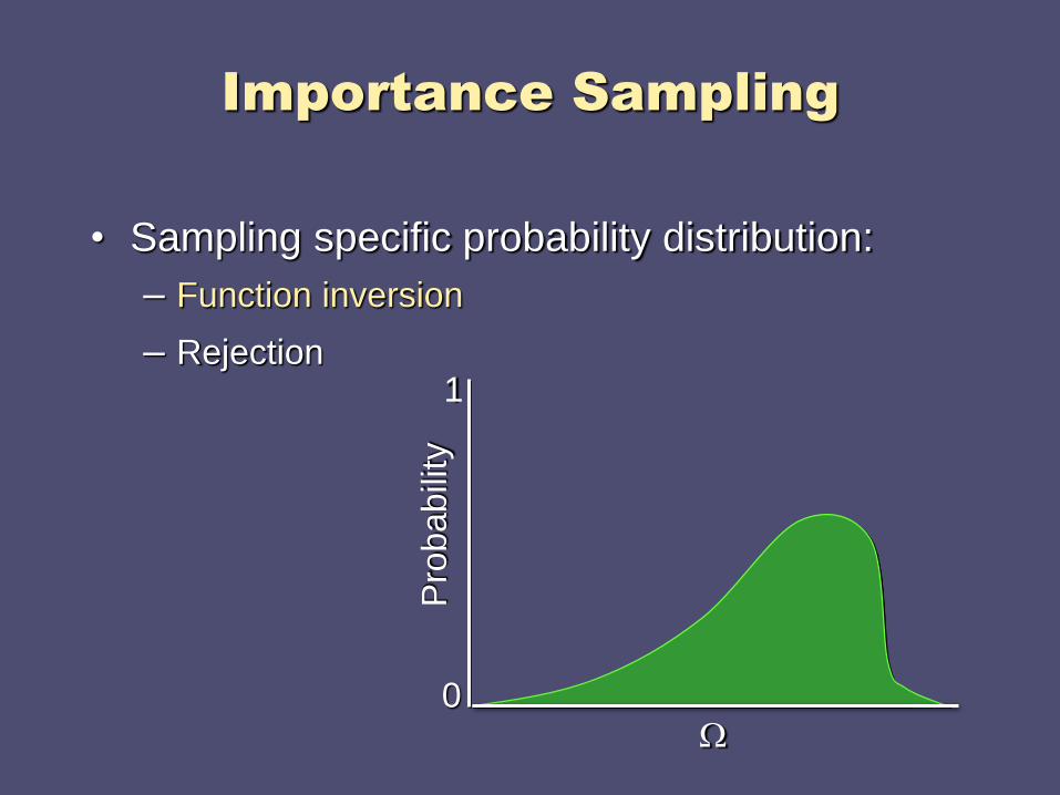
Importance Sampling
• Sampling specific probability distribution:
– Function inversion
– Rejection
Pro
babili
ty
0
1
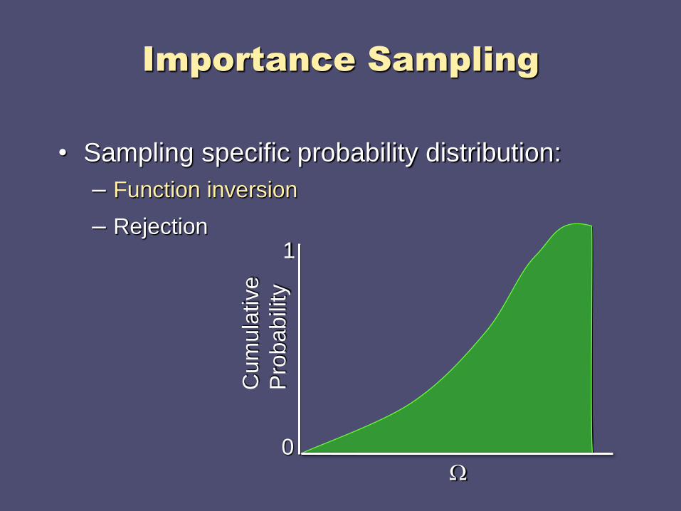
Importance Sampling
• Sampling specific probability distribution:
– Function inversion
– RejectionC
um
ula
tive
Pro
babili
ty
0
1

Importance Sampling
• Sampling specific probability distribution:
– Function inversion
– RejectionC
um
ula
tive
Pro
babili
ty
0
1
y
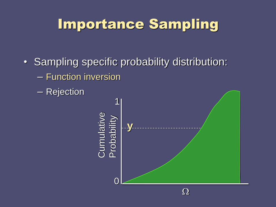
Importance Sampling
• Sampling specific probability distribution:
– Function inversion
– RejectionC
um
ula
tive
Pro
babili
ty
0
1
y

Importance Sampling
• Sampling specific probability distribution:
– Function inversion
– RejectionC
um
ula
tive
Pro
babili
ty
0
1
y
x

Importance Sampling
• Sampling specific probability distribution:
– Function inversion
– RejectionC
um
ula
tive
Pro
babili
ty
0
1

Importance Sampling
• Sampling specific probability distribution:
– Function inversion
– Rejection
Pro
babili
ty
0
1

Importance Sampling
• Sampling specific probability distribution:
– Function inversion
– Rejection
Pro
babili
ty
0
1
x
x
x
x x
xx
x
x x
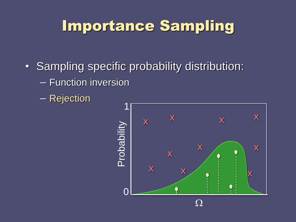
Importance Sampling
• Sampling specific probability distribution:
– Function inversion
– Rejection
Pro
babili
ty
0
1
x
x
x
x x
xx
x
x x

Combining Multiple PDFs
• Balance heuristic
– Use combination of samples generated for each PDF
– Number of samples for each PDF chosen by weights
– Near optimal
Outline
• Motivation
• Monte Carlo integration
• Variance reduction techniques
• Monte Carlo path tracing
• Sampling techniques
• Conclusion
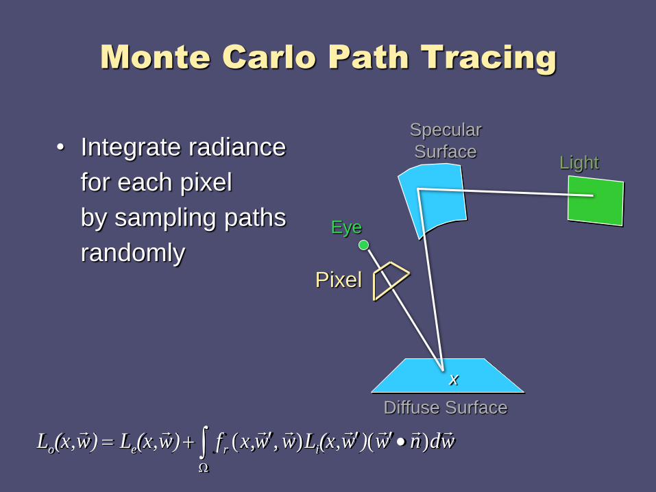
Monte Carlo Path Tracing
• Integrate radiance
for each pixel
by sampling paths
randomly
Diffuse Surface
Eye
Light
x
Specular
Surface
Pixel
wdnw)w(x,Lwwxf)w(x,L)w(x,L ireo
)(),,(

Monte Carlo Path Tracer
• For each pixel, repeat n times:
– Choose a ray with p=camera, d=(q,f) within pixel
– Pixel color += (1/n) * TracePath(p, d)
• Use stratified sampling
to select rays within
each pixel
N
i
i
UGLY
xfN
dxxf1
)(1
)(
Surface
Eye
Pixel
x

TracePath
• TracePath(p, d) returns (r,g,b):
– Trace ray (p, d) to find nearest intersection p’
– Sample radiance leaving p’ towards p
Surface
x p’
pd
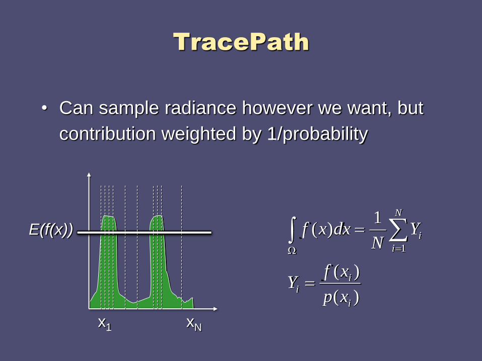
TracePath
• Can sample radiance however we want, but
contribution weighted by 1/probability
)(
)(
1)(
1
i
ii
N
i
i
xp
xfY
YN
dxxf
x1 xN
E(f(x))

• TracePath(p, d) returns (r,g,b):
– Trace ray (p, d) to find nearest intersection p’
– If random() < pemit then
• Emitted:
return (1/ pemit) * (Lered, Legreen, Leblue)
• Reflected:
generate ray in random direction d’
return (1/ (1pemit)) * fr(d d’) * (nd’) * TracePath(p’, d’)
TracePath

• TracePath(p, d) returns (r,g,b):
– Trace ray (p, d) to find nearest intersection p’
– If Le = (0,0,0) then pemit = 0
else if fr = (0,0,0) then pemit = 1
else pemit = .9
– If random() < pemit then
• Emitted:
return (1/ pemit) * (Lered, Legreen, Leblue)
• Reflected:
generate ray in random direction d’
return (1/ (1pemit)) * fr(d d’) * (nd’) * TracePath(p’, d’)
TracePath
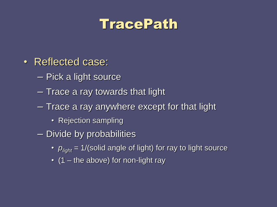
• Reflected case:
– Pick a light source
– Trace a ray towards that light
– Trace a ray anywhere except for that light
• Rejection sampling
– Divide by probabilities
• plight = 1/(solid angle of light) for ray to light source
• (1 – the above) for non-light ray
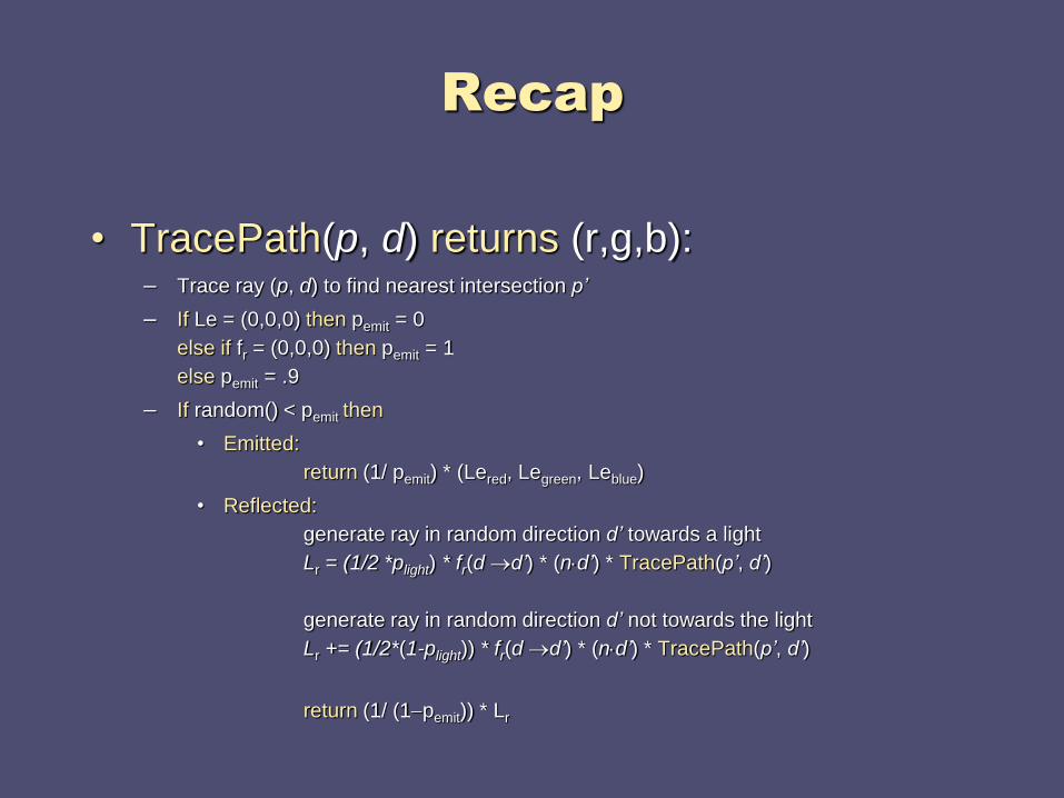
TracePath
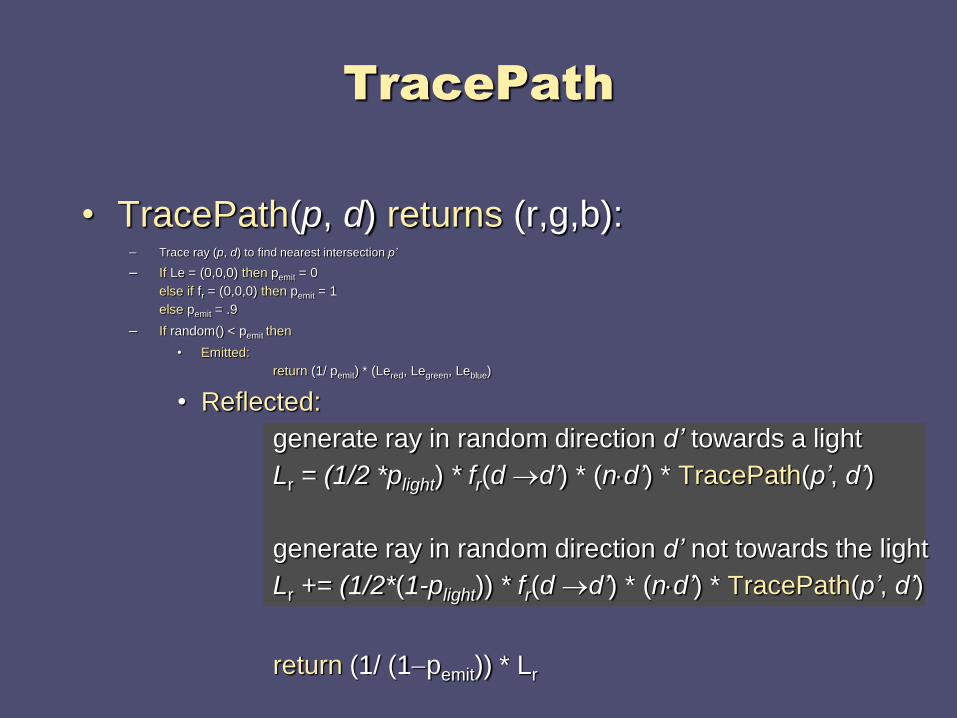
• TracePath(p, d) returns (r,g,b):– Trace ray (p, d) to find nearest intersection p’
– If Le = (0,0,0) then pemit = 0
else if fr = (0,0,0) then pemit = 1
else pemit = .9
– If random() < pemit then
• Emitted:
return (1/ pemit) * (Lered, Legreen, Leblue)
• Reflected:
generate ray in random direction d’ towards a light
Lr = (1/2 *plight) * fr(d d’) * (nd’) * TracePath(p’, d’)
generate ray in random direction d’ not towards the light
Lr += (1/2*(1-plight)) * fr(d d’) * (nd’) * TracePath(p’, d’)
return (1/ (1pemit)) * Lr
TracePath
Reflected Ray Sampling
• Uniform directional sampling:
how to generate random ray on hemisphere?
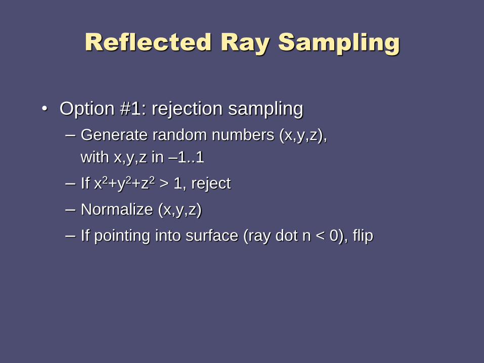
Reflected Ray Sampling
• Option #1: rejection sampling
– Generate random numbers (x,y,z),
with x,y,z in –1..1
– If x2+y2+z2 > 1, reject
– Normalize (x,y,z)
– If pointing into surface (ray dot n < 0), flip

Reflected Ray Sampling
• Option #2: inversion method
– In polar coords, density must be proportional to sin q
(remember d(solid angle) = sin q dq df)
– Integrate, invert cos-1
• So, recipe is
– Generate f in 0..2p
– Generate z in 0..1
– Let q = cos-1 z
– (x,y,z) = (sin q cos f, sin q sin f, cos q)
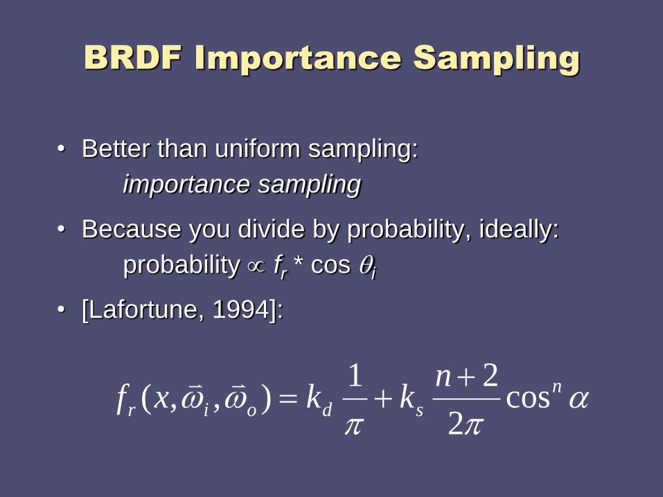
BRDF Importance Sampling
• Better than uniform sampling:
importance sampling
• Because you divide by probability, ideally:
probability fr * cos qi
• [Lafortune, 1994]:
pp
ww n
sdoir
nkkxf cos
2
21),,(
BRDF Importance Sampling
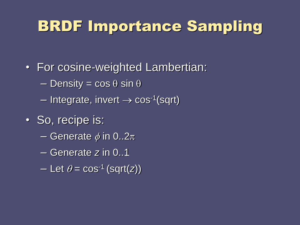
• For cosine-weighted Lambertian:
– Density = cos q sin q
– Integrate, invert cos-1(sqrt)
• So, recipe is:
– Generate f in 0..2p
– Generate z in 0..1
– Let q = cos-1 (sqrt(z))
BRDF Importance Sampling
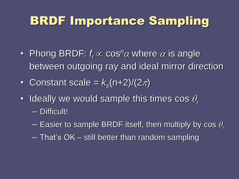
• Phong BRDF: fr cosn where is angle
between outgoing ray and ideal mirror direction
• Constant scale = ks(n+2)/(2p)
• Ideally we would sample this times cos qi
– Difficult!
– Easier to sample BRDF itself, then multiply by cos qi
– That’s OK – still better than random sampling
BRDF Importance Sampling
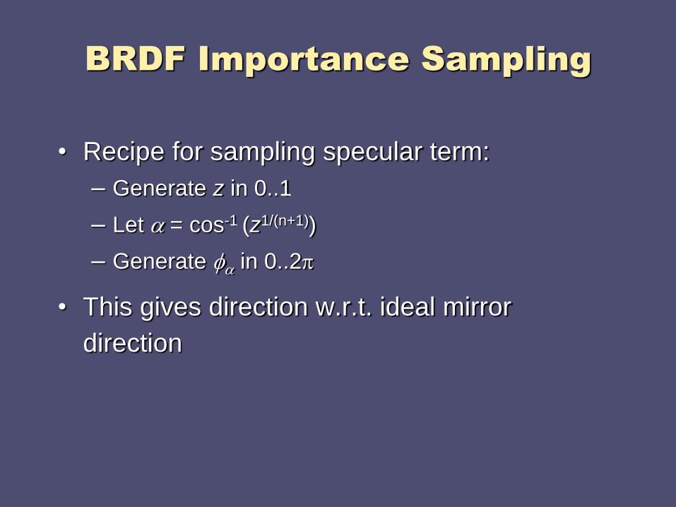
• Recipe for sampling specular term:
– Generate z in 0..1
– Let = cos-1 (z1/(n+1))
– Generate f in 0..2p
• This gives direction w.r.t. ideal mirror
direction
BRDF Importance Sampling
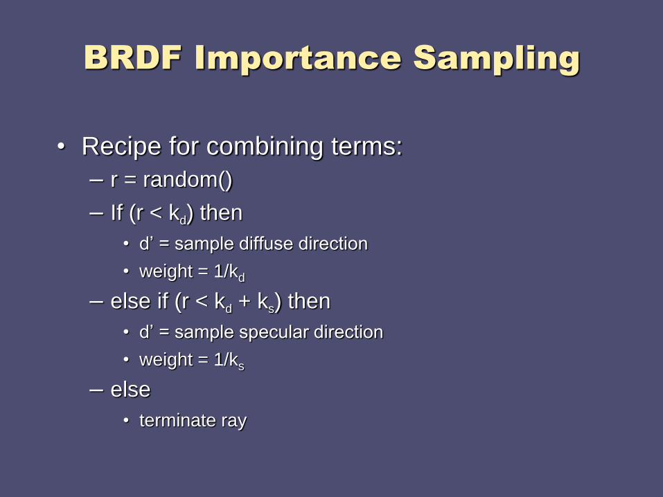
• Recipe for combining terms:
– r = random()
– If (r < kd) then
• d’ = sample diffuse direction
• weight = 1/kd
– else if (r < kd + ks) then
• d’ = sample specular direction
• weight = 1/ks
– else
• terminate ray
• TracePath(p, d) returns (r,g,b):– Trace ray (p, d) to find nearest intersection p’
– If Le = (0,0,0) then pemit = 0
else if fr = (0,0,0) then pemit = 1
else pemit = .9
– If random() < pemit then
• Emitted:
return (1/ pemit) * (Lered, Legreen, Leblue)
• Reflected:
generate ray in random direction d’ towards a light
Lr = (1/2 *plight) * fr(d d’) * (nd’) * TracePath(p’, d’)
generate ray in random direction d’ not towards the light
Lr += (1/2*(1-plight)) * fr(d d’) * (nd’) * TracePath(p’, d’)
return (1/ (1pemit)) * Lr
Recap
Monte Carlo Path Tracing
• Advantages
– Any type of geometry (procedural, curved, ...)
– Any type of BRDF (specular, glossy, diffuse, ...)
– Samples all types of paths (L(SD)*E)
– Accuracy controlled at pixel level
– Low memory consumption
– Unbiased - error appears as noise in final image
• Disadvantages
– Slow convergence
– Noise in final image
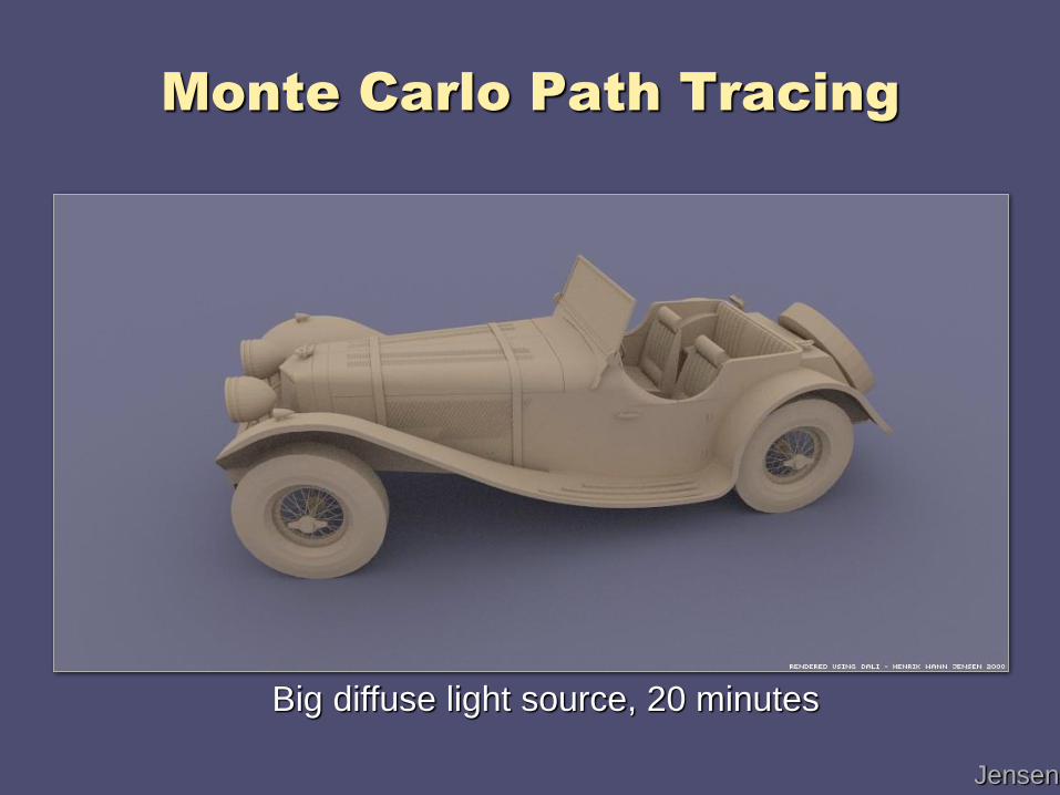
Monte Carlo Path Tracing
Big diffuse light source, 20 minutes
Jensen

Monte Carlo Path Tracing
1000 paths/pixel
Jensen
Summary
• Monte Carlo Integration Methods
– Very general
– Good for complex functions with high dimensionality
– Converge slowly (but error appears as noise)
• Conclusion
– Preferred method for difficult scenes
– Noise removal (filtering) and
irradiance caching (photon maps)
used in practice
More Information
• Books– Realistic Ray Tracing, Peter Shirley
– Realistic Image Synthesis Using Photon Mapping, Henrik Wann Jensen
• Theses– Robust Monte Carlo Methods for Light Transport Simulation, Eric Veach
– Mathematical Models and Monte Carlo Methods for Physically Based
Rendering, Eric La Fortune
• Course Notes– Mathematical Models for Computer Graphics, Stanford, Fall 1997
– State of the Art in Monte Carlo Methods for Realistic Image Synthesis,
Course 29, SIGGRAPH 2001