
MONTE CARLO CALCULATIONS OF REFLECTED …/67531/metadc131064/m2/1/high... · A solution to the...
56
MONTE CARLO CALCULATIONS OF REFLECTED INTENSITIES FOR REAL SPHERICAL ATMOSPHERES APPROVED: ' >" 'U Major Professor Minor Professor Director of the Department of Physics
Transcript of MONTE CARLO CALCULATIONS OF REFLECTED …/67531/metadc131064/m2/1/high... · A solution to the...
MONTE CARLO CALCULATIONS OF REFLECTED
INTENSITIES FOR REAL SPHERICAL
ATMOSPHERES
APPROVED: ' > "
'U Major Professor
Minor Professor
Director of the Department of Physics

MONTE CARLO CALCULATIONS OP REFLECTED
INTENSITIES POR REAL SPHERICAL
ATMOSPHERES
THESIS
Presented'to the Graduate Council of the
North Texas State University In Partial
Fulfillment of the Requirements
For the Degree of
MASTER OP SCIENCE
By-
John A. Montgomery, B»A.
Denton, Texas
January, 1969
TABLE OF CONTENTS
Page LIST OF ILLUSTRATIONS IV
Chapter
I. INTRODUCTION . . . . . . . . . . . . . 1
Motivation Problem Definition Previous Research Methodology
II. THE MODEL ATMOSPHERE . 10
Geometry Parameters
III. THE ALGORITHM . . . . . . . . . . . . 17
Photon Selection Pathlength Selection Tau Calculation Determination of the Scattering Point The Scattering Event Post-scattering Direction Cosines Detector and Local Coordinate System Flux Calculation Determination of Angular Dependence Intensity Calculation
IV. COMPARISON OF RESULTS AND CONCLUSION 35
Comparison of Results Conclusion
APPENDIX » . 40
BIBLIOGRAPHY . . 51
ill

LIST OF ILLUSTRATIONS
Figure
1. The Earth-Atmosphere System to Scale .
2. The Coordinate Systems
3. Photon Selection
Flowchart of the Scattering Simulation 4.
5.
6.
7.
8*
9.
10.
Results of Spherical Case Compared to Those of Coulson et al. forX« .1, 0 . <
Results of Spherical Case Compared to Those of Coulson et al. for X = 1, V 0
Results of Spherical Case Compared to Those of Coulson et al. for "C = 1, .8 . . .
Results of Cumulative Rayleigh Case Compared to Those of Coulson et al, for X * .1, A.," 0. ,
Results of Spherical Case Compared to Those of Adams for t • 1, 0
Results of Spherical Case Compared to Those of Adams for T e l , .8 . . . . .
Page
41
42
43
44
45
46
, 47
. 48
, 49
, 50
iv

CHAPTER I
INTRODUCTION
Motivation
There are several motivating factors leading to a study
of light scattering in spherical planetary atmospheres. These
are briefly discussed in this section, and are based upon the
importance and applicability of such a study.
Importance
A long recognized need in radiative transfer theory has
been the development of a solution to the problem of light
scattering in spherical planetary atmospheres. This need is
discussed by 0. I. Smoktli (13). A successful technique must,
in effect, solve the transfer equations for a spherical model
sufficiently complex as to approach reality. It should
accurately predict and explain phenomena arising from atmos-
pheric sphericity.
Applicability
Such a solution to the spherical problem would have
application to a myriad of atmospheric scattering phenomena.
An extension of the understanding of the earth"s atmosphere
might become possible due to the greater realism of the

model considered—a model capable of involving numerous
light-scattering processes and atmospheric sphericity.
A solution to the inverse problem becomes feasible If
one has a means of calculating emergent radiation as a
function of atmospheric parameters. The inverse problem
is the determination of meteorological quantities such as
temperature from external measurements of emergent radiation,
and might have utility in the solution of the Venus problem.
Problem Definition
Before proceeding, the spherical problem as considered
herein must be defined. The intended quantitative determi-
nation, parameterization, and problem restrictions are
expressly delineated.
Desired Determination
To calculate the emergent radiation field, a realistic
atmospheric model and algorithm must be developed. The radi-
ation field may be characterized by the emergent intensities
of scattered light. This is possible only if the algorithm
determines these intensities as dependent upon atmospheric
and angular parameters.
Parameters
The parameters to be considered are as follows:
1. The total optical thickness of the atmosphere.
2. The altitude-dependent extinction coefficients.
3. The altitude-dependent cross-sections.

4. The albedo of the planet surface.
5. The angular dependence of the emergent
intensities.
Restrictions
This solution to the spherical problem is restricted by
several simplifying assumptions.
Atmospheric parameters are considered constant over radial
distanoes that are small compared to the atmospheric thickness.
The ground is taken as a homogeneous Lambert surface, although
different albedoes may be used. Uniform incident solar flux
is assumed, where the flux is normalized to unity over an area
perpendicular to the direction of incidence. Further simplifi-
cations are made by assuming azimuthal symmetry with respect
to the incident direction, and by disregarding polarization
effects.
Previous Research
There are many references in the literature to research
on light scattering in planetary atmospheres. These reports
are primarily concerned, analytically and numerically, with
the plane-parallel approximation. To date, most attempts to
formulate and solve the spherical problem have been largely
unsuccessful. The two approaches are considered in turn.
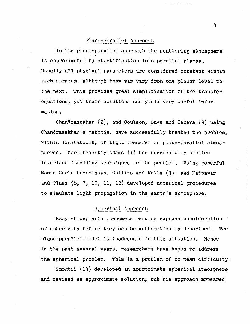
Plane-Parallel Approach
In the plane-parallel approach the scattering atmosphere *
Is approximated by stratification into parallel planes.
Usually all physical parameters are considered constant within
each stratum, although they may vary from one planar level to
the next. This provides great simplification of the transfer
equations, yet their solutions can yield very useful infor-
mation.
Chandrasekhar (2), and Coulson, Dave and Sekera (4) using
Chandrasekhar's methods, have successfully treated the problem,
within limitations, of light transfer in plane-parallel atmos-
pheres. More recently Adams (1) has successfully applied
invariant imbedding techniques to the problem. Using powerful
Monte Carlo techniques, Collins and Wells (3), and Kattawar
and Plass (6, 7, 10, 11, 12) developed numerical procedures
to simulate light propagation in the earth's atmosphere.
Spherical Approach
Many atmospheric phenomena require express consideration *
of sphericity before they can be mathematically described. The
plane-parallel model is inadequate In this situation. Hence
in the past several years, researchers have begun to address
the spherical problem. This is a problem of no mean difficulty,
Smoktii (13) developed an approximate spherical atmosphere
and devised an approximate solution, but his approach appeared

to be cumbersome and of limited utility. A valuable algorithm
for two classes of problems has been developed by Marchuk and
Mlkhailov (8, 9) at Novosslblrsk.
Comparison of the Two Approaches
The plane-parallel and spherical approaches have certain
relative advantages.
The plane-parallel approach has the advantage of producing
a simpler mathematical representation with correspondingly
simpler solutions. However, the plane-parallel model is
representative of reality only over short lateral distances,
has singularities in the equations for unit albedo, and is
unable to describe some of the more interesting facets of
atmospheric radiation, such as twilight phenomena.
The spherical Approach provides a more realistic model,
capable of including most atmospheric phenomena. If Monte
Carlo techniques are applied the complexity of the model is
limited primarily by practicality. Even using the Monte Carlo
method the spherical equations of transfer are very difficult
to solve.
Methodology
In this section the methods used, together with the reasons
for their selection, will be discussed.

Model
The purpose iB to develop a realistic spherical model
which utilizes commonly used atmospheric data. This model
has several strong likenesses to the plane-parallel one
after sphericity is discounted, providing a means of com-#
parison to the analogous plane-parallel case.
The model includes two basic types of atmospheric
scattering—Rayleigh scattering, which is molecular, and
Mie scattering from spherical aerosols. For Mie scattering
it is assumed that the dielectric constants of the Individual
particles are known; hence the scattering indicatrioes may
be determined.
Algorithm
The algorithm developed relies heavily on Monte Carlo
simulation of the scattering processes. These processes are
essentially a finite Markov Chain. The method computes the
emergent intensities of light which experiences multiple
scattering and reflection. Rayleigh, Mie, and Lambert events
are considered.
A general discussion of Monte Carlo techniques and their
development is given by Hammersley and Handscomb (5), but is
beyond the scope of this paper. Some important considerations
are discussed, however.
The Monte Carlo technique is applicable to a problem
which consists of a sequence of events where the probability

for the occurrence of each event is known. The sequence may
be simulated by Monte Carlo and the total probability for all
events determined. Light scattering in an atmosphere is such
a sequence; hence the Monte Carlo method is applicable.
As discussed by Plass and Kattawar (11, p. 415), the
Monte Carlo method applied to radiative transfer problems
has these advantages:
1. The atmospheric parameters may vary with
height in any desired manner.
2. Any scattering function may be considered
regardless of the anisotropy,
3. The angular distribution of surface-scattered
radiation may be varied.
4. The number of detectors and angles where
intensities are determined Is limited only
by practicality.
However, a disadvantage of the method is that the standard
deviation of the results is inversely proportional to the
square root of the computing time.
CHAPTER BIBLIOGRAPHY
1. Adams, Charles, "Solutions of the Equations of Radiative Transfer by an Invariant Imbedding Approach," unpublished master's thesis, Department of Physics, North Texas State University, Denton, Texas, 1968.
2. Chandrasekhar, S., Radiative Transfer, New York, Dover Publications, Inc., I960.
3. Collins, D. G. and M, B. Wells, Monte Carlo Codes for Study of Light Transport in the Atmosphere, Vol. I, 2 volumes, Fort Worth, Radiation Research Associates, Inc., 1965.
4. Coulson, K. L., J. V. Dave, and Z. Sekera, Tables Related to Radiation Emerging from a Planetary Atmosphere with Raylelgh Scattering. Berkeley. University of California Press, 19<5<n
5. Hammersley, J. M. and D. C. Handscomb, Monte Carlo Methods, New York, John Wiley and Sons, Inc., 1964.
6. Kattawar, G. W. and G. N. Plass, "Electromagnetic Scattering from Absorbing Spheres," Applied Opticss VI (August, 1967). 1377-1382.
7. Kattawar, G. W. and G. N. Plass, "Resonance Scattering from Absorbing Spheres," Applied Optics, VI (September, 1967). 1549-1554.
8. Marchuk, G. I. and G. A. Mlkhailov, "Results of the Solution ' of Certain Problems of Atmospheric Optics by the Monte Carlo Method," Izv,, Atmospheric and Oceanic Physics, III (1967), 227-231.
9« Marchuk, G. I. and G. A. Mikhailov, "The Solution of Problems of Atmospheric Optics by a Monte Carlo Method," Izv., Atmospheric and Oceanic Physics, III (1967), 147-155.
10. Plass, G. N. and G. W. Kattawar, "influence of Single Scattering Albedo on Reflected and Transmitted Light from Clouds," Applied Optloa. VII (February, 1968), 361-367.
8

11. Plass, G. N. arid G. W. Kattawar, "Monte Carlo Calculations of Light Scattering from Clouds," Applied Optica, VII (March, 1968), 415-419.
12. Plass, G. N. and G. W. Kattawar,"Radiant Intensity of
Light Scattered from Clouds," Applied Optics, VII (April, 1968), 699-704.
13. Smoktli, 0. I., "Multiple Scattering of Light in a 1(
Homogeneous Spherically Symmetrical Planetary Atmosphere, Izv., Atmospheric and Oceanic Physics, III (1967)# 140-146.
CHAPTER II
THE MODEL ATMOSPHERE
The model atmosphere considered herein la a spherical
shell concentric with the planet, and of finite extent. The
ratio of atmospheric radius to planetary radius is sixty-five
sixty-fourths, corresponding to 6500 kilometers and 6400
kilometers respectively for the earth. Arbitrary units may
be used, as in this calculation, as long as the proper ratio
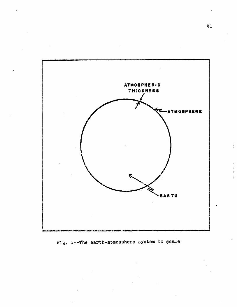
is preserved. In Figure 1 the model cross-section is shown
to scale. The comparative thinness of the atmosphere empha-
sizes the fact that its curvature must be considered in a
realistic model.
Geometry
Figure 2 is a representation of the atmosphere-earth
system with the atmospheric thickness exaggerated for clarity.
Although only the upper hemisphere Is shown, the model includes
the entire sphere.
All coordinates and direction cosines are determined relative
to a coordinate system fixed in the planet, as shown in Figure 2.
Points are specified in either cartesian or spherical coordinates
as dictated by ease of determination*
10
11
The solar flux is Incident on the negative-x hemisphere
in a direction parallel to the x axis. It is assumed parallel,
unpolarized, and of unit strength.
Zone Structure
The atmosphere is divided into ten concentric spherical
zones which are analogous to the parallel planes of the plane-
parallel model.
Each .zone is referenced by the index of the outermost
radius of the zone. That is, the 1-th zone oontalns all points
of radius r such that
Ri-1* r i Ri*
The planet surface is considered the inner boundary of the
first zone.
All zones have nearly the same optical thickness
but different physical thicknesses. For a total atmospheric
optical thickness X , it is required that
i -i - i
The atmospheric parameters are considered constant within
each zone, but may vary from one zone to the next.
Detector Bands
The outer rim of the atmosphere is divided into five
detector bands. These bands are of equal width in ,
where JJ^is the cosine of the nadir angle . Equal spacing

12
in ensures that the detector bands have equal areas. The
assumption of azlmuthal symmetry relative to the incident
direction requires that all points with the same f L in a
given detector band are equivalent. Although those with
different are not equivalent within a given band, practi-
cality requires that they be treated as such.
The detector bands allow determination of the angular
dependence of emergent intensities on the planet nadir
angle ©0, where ©o is shown in Figure 2. Any reasonable
number of bands may be used.
Local Coordinate System
To determine the angular dependence of the emergent
intensities at the points of emergence, local coordinate
systems are constructed at these points. In these local
systems the angular dependencies may be ascertained.
A local coordinate system with origin at the detector
point is shown in Figure 2. The local x'y1 plane is tangent
to the atmospheric rim, and the z1 axis is outwardly normal.
The x' axis is required to be in a plane containing the radius
vector to the point of emergence, and the planet x axis. This
x1 axis is so directed that the incident flux makes a local ft
angle of zero relative to it.
As it is impossible to determine the angular dependence
in the local system on all possible angles of emergence, the
13
local system Is divided into a finite number of angular
bins. All emergent photons passing through a given bin
are treated as equivalent.
The bins are determined by the cosine of the local
zenith angle 9, while the & bins are determined by the local
azimuth angle,0, As azimuthal symmetry is assumed for the
model atmosphere, no distinction need be made as to which
side of the x® axis the 0 bins lie.
Parameters
It is now apropos to discuss the means of determining
the atmospheric parameters which describe the model atmosphere.
Tau
The total atmospheric d e p t h m a y be specified as any
reasonable value. For the calculation they range from one-
tenth to ten.
Extinction Coefficients
The atmospheric extinction coefficients are determined
by the method of Collins and Wells (1/ p. 22) „ Once ti is
selected, the extinction coefficient of each zone may be
computed in the following manner. Let h be the height
above the planet surface, and £(h) the extinction coefficient
at h. The dependence of C on h is given by
C(h) « oce~Bh,
where ocis determined by ^ , and B is a constant•determining

14
the height dependence of atmospheric density. Beta is taken
as 0.0125 for the earth, hence
E(h) = C C e " °, 0 1 2 5 h .
Alpha is determined by the requirement that
where h1 is the maximum height of the atmosphere, and B
is positive. This has the solution
^ » { <VB) e~ B h * «/k.
Taking the limit as h increases without bound, and solving
for ce 3 we find that
CL - 0.0125^ v
Hence,
E(h) - 0.0125Ue"*0,0125h.
The extinction coefficient of each zone, may be ' i
determined by picking the S ( h ) within eaoh such that the
relationship 10
t ( E i t t) X S5 *"
is satisfied, where t 1 is the physical thickness of each zone,
Proas-sections
The cross-sections for Rayleigh and Mie total scattering
and absorption are determined by physical measurements.

15
Scattering Functions
The scattering functions for aerosols are those computed
by Kattawar and Plass (2). Their computational method is
discussed in the article.
Albedo
The earth's surface albedo may be varied according to
calculatlonal need. However, an albedo of eight-tenths is
usually assumed for the earth.
CHAPTER BIBLIOGRAPHY
1, Collins, D. G. and M. B. Wells, Monte Carlo Codes for Study of Light Transport in the Atmosphere, Vol. II, 2 volumes, Port Worth, Radiation Research Associates, Inc., 1965.
2. Kattawar, G. W. and G. N. Plass, "Electromagnetic Scattering from Absorbing Spheres," Applied Optics, VI (August, 1967), 1377-1382.
16

CHAPTER III
THE ALGORITHM
The algorithm which simulates the light scattering
process Is described In this chapter. Implementation of
the algorithm Is effected by a program written for an
International Business Machines 360/50 Computer.
The separate computations required are presented
approximately in their order of performance in the simu-
lation process. This is done because each computation is
logically dependent on those preceding It.
Rejection techniques used to model the theoretical
distribution functions have been tested separately before
inclusion In the program. These techniques use the multi-
plicative congruentlal random-number generator provided in
the International Business Machines Scientific Subroutine *
Package.
Several variance-reducing techniques are used in the
algorithm. Each technique has two parts. These are sampling
from a biased distribution, then removing the bias. The
distribution Is biased in a way which increases the number
of events occurring In regions of Interest. Such a bias effec-
tively Increases the population of events in the desired region,
IT
18
thus decreasing the variance. This bias must be removed
after the desired computations have been performed in
order to preserve reality. The bias removal is effected
by assigning to each event a statistical weight determined
by the true probability of its occurrence. Examples of
this may be seen in the photon and pathlength selections.
Photon Selection
The first step in simulating the scattering sequence
is the selection of a photon to be followed. Both its
direction and coordinates must be chosen.
Each photon is incident in the positive x direction
in the planet system. Hence If we let S be a unit vector
in the photon direction* A ^ Jf% A S « & ^ ^ly + ®
where a, b, c are the direction cosines of § in the planet
system. For the inoident photon b and c are zero while
a is unity.
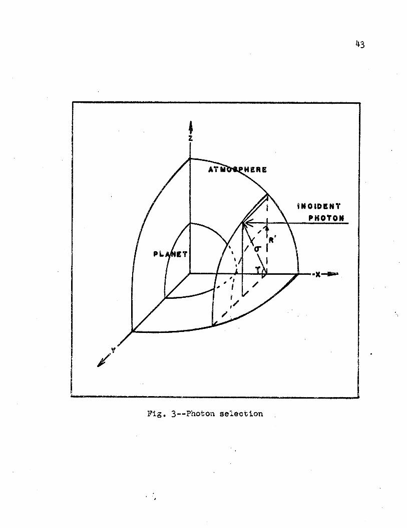
Assuming uniform incident flux and azimuthal symmetry,
a photon has uniform probability of incidence on any element
of a plane area perpendicular to S. As the photon Is actu-
ally incident on the atmosphere, it must be incident on the
rim of a disk of radius cr , perpendicular to S. This radius
must be determined as shown in Figure 3•
For Increased flexibility it is desired to be able
to bias the ©"distribution so that <r may be selected in
19
the range
R ' £ <r £ RA,
where R! Is in the range
0 £ R' < RA,
and R a is the radius of the atmosphere. Requiring that
A
n 2<rd<r - 1 , 'R'
one finds that , 2 o -1
N * (Ra - R' ) .
Hence, we may require that
CT • (CR2- R I 2)(R a2 - R*2)"1,
where CCis a random number in (0,1). Solving this
expression for 0* , the distribution-modelling formula is
found to be
0" 88 (R1 + &(RA2 " R'2) )*.
This reduces to the formula of Marchuk and Mikhailov (3, p.152)
when R® is zero. #
For R$ not zero, sampling <f in this manner introduces
bias into the calculation. The bias may be removed by a
statistical weight factor, w. If P( 0*) is the probability
of choosing 0* in (0, R A) and P'(0~) is the probability of
choosing CTln (R',RA), then the weight factor is given by
W - P( C)/P ' (Cr ) . :

20
Now
P (<r) dor a 2<t/ra2
and P'(<T) dflT- 2<T/(RA2 - R«2),
hence W * 1 - R,2/Ra2*
For R1 equal to zero the weight is unity. Not only does this
allow a shifting of <T as desired, but it also has the effeot
of reducing the variance in certain regions of interest.
To completely specify the point of incidence, an
azimuthal angle must be chosen. If T is the angle between O" and
the planet y axis, then T must be uniformly distributed in (0,21T).
Gamma is specified by
sinT * sin (2TT<£ ),
cos Tf - cos (2*trc),
where <C is a random number in (0,1). The coordinates of the point
of incidence (x,y,z), are given by
x • - ( r a 2 ~ < r 2 ) K
y " <rcos*f ,
z • qrsinf . «
This is shown in Figure 3.
Pathlength Selection
To decrease the computational time it is necessary to
require that no photon escape the atmosphere. If this is not
done a significant number of incident photons esoape before
experiencing a oolllsion. The requirement is satisfied In the
determination of P, the optical pathlength traversed by a photon
21
before collision. Two exponential distributions In optical
pathlength are used, one of which is truncated to ensure
that the photons remain within the atmosphere.
If a photon moving in direction § sees the planet along
its path, the unbiased exponential distribution is used. In
this case the photon cannot escape without scattering either
in the atmosphere or from the ground. Solving the equation
.P
flt • I -p« e dP®,
o
where <£ is a random number, gives a means of sampling from
this distribution. The solution for P is
P » -ln(l-<).
If £ is distributed uniformly in (0,1), then (1- (t ) is
distributed uniformly in (0,1). Hence P » -ln( <£).
A means of sampling from the truncated distribution
is needed when the photon does not see the planet along its
path, and could thus escape. This is accomplished by solving
the equation P ~PS
e 1 - e-T max
<£ . ^ e dPs
where is the total optical pathlength through the v ulc&X
A
atmosphere along S. The solution for P is
p . - m (1 - <t(l - e - W ) )
which, in the limit as X max i n c r e a s e a without bound, yields P . -In (1 - * )
as before.

22
Sampling from the truncated distribution introduces a
removable bias. The bias is removed by assigning an initial
statistical weight, w equal to unity, to the incident photons.
Each time P is sampled from the truncated exponential distri-
bution, the photon's statistical weight is reduced by the mX
factor (1 - © m a x ) . This is the probability that a collision
will occur before the photon escapes the atmosphere.
The above method is described by Cashwell and Everett (l).
Tau Calculation
The optical pathlength T , traversed in passing through
the atmosphere zones, is used in the selection of P, determi-
nation of the statistical weight, computation of scattering -
point coordinates, and calculation of emergent fluxes. A
large proportion of' the total computing time is required for
the tau calculations; hence they must be performed in the
optimal manner.
The calculations fall into two classes. These classes
involve the strictly outgoing photon and the incoming photon.
Only -the most general method within each class is discussed.
Let R a be the radius of the point where a photon begins
moving in the § direction, and let £ a be a unit vector along R g.
A photon is said to be strictly outgoing If
cos^to >
where A f*
COS • Rg* S.
Otherwise, the photon la said to be incoming.
23
Outgoing Photon
In this case t is computed by a method given by
Mateer (4), Let H * RS - RT ,
5 • cos"*1 (Rj* §),
K » (1 • H/R8 )sin5 .
The distance from R| to the i-th zone boundary along S is
given by
DT - (R? - K 2 R | )i - ( R | - K%2 ) * ,
where i is the index of any zone whose R^ is greater than
R S . If j is the index of the innermost zone whose Rj is a
greater than the total optical pathlength along S is
given by
X * fri , <Di " Di-i)Ei+DjEr max l *** J *
Incoming Photon
The treatment of incoming photons is more complicated,
as in this case the photon may penetrate each zone more than
once.
Let D be the distance of closest approach of an ca
incoming photon to the origin of the planet system, where
D c a * R$ I sir.5 1.
Further, let D H e within the j-th zone. Define Pc as ca
the point in the k-th zone where the photon began moving
in the S direction, and L to be the distance between

2k
and PQ such that
t - (R2 - D§a)i.
It is desired to begin at Pn and move towards D„Q w C o
A along S, computing theti traversed in each zone. The
optical pathlength.traversed in the k-th zone is given by
2 .4
k* (L - (Rfj-l - D o a)
5)E
D is the distance traversed in the \ th zone, where « P L
D| = L - (H^ 1 - D c a)2.
Thus D 1E 1 .
This procedure is followed until the incoming photon
reaches the D c a. On the outgoing side, Mateex's method (4)
may be used to compute the remainder of "£max.> Hence m a x
ia the sum of the T! 's on the inooming side and those on the
outgoing side.
Determination of the Scattering Point
Once the optical pathlength to collision, P, has been
determined, the coordinates of the scattering point may be
calculated. This is effected by computing the the photon
sees along beginning at PQ. At each zone the cumulative
is compared to P and the distance, D, accumulated. If TJ
is less than P the calculation continues until a value is
reached such that % is greater than, or equal to, P. Hence
if X becomes greater than, or equal to, P in the i-th zone,

25
the total physical distance along S to the scattering-point
is DT = D - { % - P)/Ci.
The coordinates of the scattering-point are given by
X • x + aQ,, ,
Y • y ^ bQj. ,
Z = z * 0 % ,
where (x, y, z) are the coordinates of P0, and (a, b, c) are
the direction cosines of
The Scattering Event
Three types of scattering events may occur in the model
atmosphere. The means of determining the scattering type,
and of modelling the scattering event is discussed in this
section.
Determination of Scattering Type
The three types of events fall into two scattering
classifications—ground scattering and atmospheric scattering.
If during the computation of the scattering-point coordinates
the photon strikes the ground while TJ is less than P, a ground-
scattering event is said to occur. Ground-scattering events
are treated as Lambert scattering events, while atmospheric
scattering may be either Rayleigh or Mie.
The means of selecting the type of atmospheric scattering
is described by Collins and Wells (2, p. 38). To determine
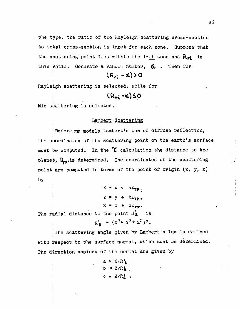
26
the type, the ratio of the Rayleigh scattering cross-section
to total cross-section is input for each zone. Suppose that
the scattering point lies within the i-th zone and is
this ratio. Generate a random number, & . 'Then for
( R p i - c t ) > 0
Rayleigh scattering Is selected, while for
i r k -<0 i o
Mle scattering Is selected.
Lambert Scattering
Before cne models Lambert's law of diffuse reflection,
x>rdinates of the scattering point on the earth's surface
le computed. In the % calculation the distance to the
, C^,is determined. The coordinates of the scattering
are computed in terms of the point of origin (x, y, z)
the c
must
plane
point
by
X * x * aD^p
Y - y 4- bD-yp, s
Z * z + cDtp «
The radial distance to the point R$ is
| - (X2^ Y 2* z2)h
The scattering angle given by Lambert's law is defined
with respect to the surface normal, which must be determined.
The direction cosines of the normal are given by
a - X/R'a ,
b • Y/R^ >
c . Z/Rl .
27
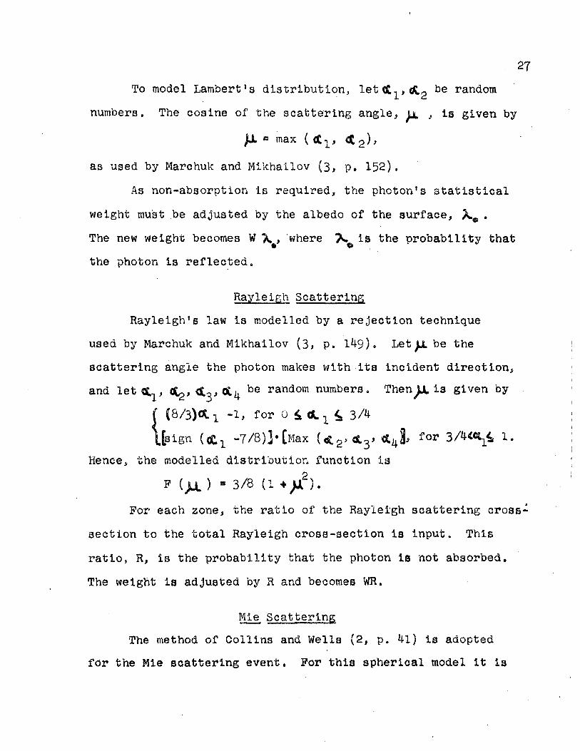
To model Lambert's distribution, let cC^, <£2 be random
numbers. The cosine of the scattering angle, jjL , is given by
JJL • max ( <t1, <t2),
as used by Marchuk and Mikhailov (3, p. 152).
As non-absorption is required, the photon's statistical
weight must be adjusted by the albedo of the surface, X , .
The new weight becomes W \ #, where Is the probability that
the photon is reflected.
Rayleigh Scattering
Rayleigh's law is modelled by a rejection technique
used by Marchuk and Mikhailov (3, p. 1^9). Let JL be the
scattering angle the photon makes with its incident direction,
and let oCg, b e random numbers. T h e n i s given by
( C 8 / 3 K 1 -1, for 0 £ «L 1 3 A
\[slgn (c£1 -7/8)]'[Max (* 2> diy for 3 / W ^ 1.
Hence, the modelled distribution function is
F (JUL ) " 3/ 8 U + >A2).
For each zone, the ratio of the Rayleigh scattering cross-
section to the total Rayleigh cross-section is input. This
ratio, R, is the probability that the photon is not absorbed.
The weight is adjusted by R and becomes WR.
Mle Scattering
The method of Collins and Wells (2, p. 4l) is adopted
for the Mle scattering event. For this spherical model it Is

28
possible to have as many Mie functions as zones. The index
of the zone in which the Mie scattering occurs is the index
of the Mie function to be used. The variety of Mie functions
allows the inclusion of different types of Mie scattering
within the same mo£el. For example one may have different
types of clouds at various layers in the atmosphere.
The cumulative Mie scattering angular distribution is
input for each Mie function. The scattering angle is selected
from this distribution. For each zone there are gs| possible
values k j. These are computed such that there is equal
probability between^JLk j and Jl T h e l n d e x i s determined
such that
(J-l)/ N k £ <£ <, J/Kk,
where cC is a random number. The cosine , / x , of the scattering
angle relative to the incident direction is determined by inter-
polating linearly between JJL and ^ ^ j.
For the zone in which the photon is scattered, the ratio
of the Mie scattering cross-section to the total Mie cross-
section is input. This ratio, R M , is the probability that
the photon is not absorbed. The statistical weight is adjusted
by and becomes WR^.
Post-Scattering Direction Cosines
After collision an azlmuthal angle must be selected and
new direction cosines determined.

29
Aa azimuthal symmetry Is assumed the azimuthal angle
must be selected In the interval (0, 2TT) In a plane perpen-
dicular to the Incident direction. Note however, that for
Lambert scattering the incident direction is taken to be the
outward normal to the scattering surface. The azimuthal
angle,p , is specified by
sin$f • sin (2TT<t),
cos0 a cos (2TTQL),
where & is a random number.
The new direction cosines may now be computed using the
method of Marchuk and Mikhailov (3, p. 149). Let S be the
pre-scattering direction denoted by
S 2£ • bly ^ f
and the new direction specified by
S1 = a'lx* b«ly4-c»lz.
L e t b e the cosine of the scattering angle. Define
(1 - } 1 2 F CO3 0 ,
(1 -p?)1 strip ,
k s as,.- bgg,. The new direction cosines are now given by
a8 = - K/(14 lcl)3V
b« s b[jJL - K/(l + lolfl
c« j. • k sign (c).

3°
Detector and Local Coordinate System
If D Is the distance along S to the rim of the atmosphere,
then the coordinates of the detector point are given by
x 0 * x aD,
y 0 = y + hD,
Z p S SS cD,
where (x, y, z) is the scattering point and (a, b, o) are the
new direction cosines.
The local coordinate system has origin at the detector
point and is subject to previously discussed requirements.
It is necessary to specify mathematically the local x1, y', z1
directions in the planet system. The 1 . direction is known z
to be normal to the atmospheric surface and is in the &
direction, where 1 is the unit vector towards the point R
y#J z§). Now
i ly
and
* ^ R * 1X^
A A
V - V* V hence
a
Sc* ~ x XR *> /* ^ v« 1v' " ^1R* l±' R*
where * , A A LH
Performing this, one finds that *
lp • ^D^x ^ V * *D
ix. = (yp • zl > - ( x
Dyp) - t ' p V V
p2 ®2 «2 RD RD KD

31
A ^
In general 1„, Is not a unit vector. Normalizing, 1„. is
found to be (yj * z d ^ i* - (xpyp) V - (xpyp) V
rD Rp(yp zp)^ Rp(yp+ zp)^
A \ A, The coefficients of lx„ ly, lz are the direction cosines
, . A
(d|, b|, C|), of lxi in the planet system. Hence the local
coordinate system is completely specified.
Flux Calculation
After each collision where the photon is directed outward,
a flux contribution to the detector penetrated is computed.
This raw flux, FR, is computed by
pH - w e ,
A where If is the optical pathlength to the detector along S and
-t
W is the statistical weight. The factor £ is the probability
that the photon reaches the detector without scattering.
Petermination of Angular Pependence
The angular dependence of the emergent flux in the local
system Is now determined. The cosine,p. , of the angle the
emergent flux makes with the local zenith is given by H A
)k = S • lzt, ' *
where ya is the oosine of 9, The projection of S on the x«

32
axis Is
Sx, » t* lx, = aa% «• bb% *• oc%, A
where S Is the direction of the emergent flux» However,
sx« Is also given by
1§1 sin 9 cos
where
sin 9 = (1 -)l2)K
The cosine of the local azimuthal angle, 0, is given by
cos 0 = (aa 4» bb * cc^)/sln 9,
for sin 9 not zero. If sin 9 is zero, cos # is taken to
be unity. The angle $ is given by
$ a cos [(aa^ * bb^ • CC| )/sin 9^ .
The cosine,^ , of the planet nadir angle is determined
by comparing the x coordinate of the detector point with the
x boundaries of the detector bands.
Once the angular dependence of the fluxes has been
determined, the fluxes are recorded In bins according to their
angular dependence.
Termination
The photon continues this scattering cycle, as shown by
the flow chart given in Figure 4, until its weight drops below
a termination criterion. When this occurs the photon is
terminated, a new one selected, and the process begins anew*

33
Intensity Calculation
After the desired number of photons have been processed,
the Intensities of the emergent radiation are computed from
the fluxes,
Let Fr be the total raw flux. The average flux
contribution per photon is given by
P * Fr/2.Nh*)Ao,
where the width of the detector bands. The effective
number of photons considered,N Is
N /(I - R'2/RI ),
as defined for photon selection and N is the number of
histories processed.
The intensity may now be computed from the flux.
Solving the equation
P . yidjjLcty
For I, which is assumed constant over a interval, yields
I - 2F/ [(02 ~ *
The 0 values only cover the interval (0, IT )] hence
X - F/Kfc, -0l)(>jf2 - M* )3 •
With little extra effort the intensity Is determined
for the case when the albedo Is zero, regardless of the
albedo assumed for the planet. This Is effected by separately
recording the flux contributions of photons that have not yet
experienced a Lambert reflection.
CHAPTER BIBLIOGRAPHY
1. Cashwell, E. D. and C. J. Everett, Practical Manual on the Monte Carlo Method for Random Walk Problems, New York, Pergamon Press, Inc., 1959.
2. Collins, D. G. and M. B. Wells, Monte Carlo Codes for Study of Light Transport In the Atmosphere, Vol. I, 2 volumes, Port Worth, Radiation Research Associates, Inc., 1965.
3• Marchuk, G. I. and G, A. Mikhailov, "The Solution of Problems of Atmospheric Optics by a Monte Carlo Method,' Izv., Atmospheric and Oceanic Physios, III (1967)* 147-155.
4, Mateer, C. L.', 'Laboratory of Atmospheric Sciences, Boulder, Colorado, letter, March, 1968,
3 4
CHAPTER IV
COMPARISON OP RESULTS AND CONCLUSION
Comparison of Results
No spherical results have been given in the literature
that are suitable for comparison to the values obtained
from this calculation. However, f o r b e t w e e n 0.40 and
0.80, the results obtained from this spherical model should
have very nearly the same values as those obtained from the
similar plane-parallel model. Comparisons will be made to the
well substantiated results of Coulson et aL (2) and Adams (1).
These results are determined within different 0 bins, As the
values of the reflected intensities are not strongly 0 depen-
dent, all results are averaged over 0 .
Results Compared to Those of Coulson et al.
Even though Coulson1s results (2) are for the vector
case, the results of the spherical calculation should closely
approximate them.
The Coulson and spherical results are compared in Figure 5
for the case » 0.10 and 0. For * 0.80, the histogram
showing the spherical results is much lower than the Coulson
curve for JL near the looal horizon, becoming slightly higher
35

36
near the zenith. A lower intensity is expected for the
spherical model in the region^JL* a s this includes
a much smaller volume of space than does the plane-parallel
model for JJL = 0.10. For |JL • 0.40, the plane-parallel
intensity is again larger for jx • 0.10 and slightly smaller
for towards the zenith. The overall agreement of the two
models is excellent.
Figure 6 shows the results of Coulson et_ aL compared
to the spherical results for the case X • 1.00 and ^ • 0.0.
The s 0.80 histogram shows excellent agreement with the
Coulson curve for yi greater than 0.20, and the expected lower
intensity near the horizon. For JJl » 0.40, the histogram
again shows the same type of agreement with Coulson's values.
The spherical results are compared to Coulson8s in
Figure 7* for the case X « 1.00 and « 0.80. The JUL - 0.80
histogram shows good agreement with Coulson's curve, especially
in the range from - 0.20 to JJL - 0.80. The elevated
value for jx » 0.80 to 0.90 is probably just a statistical
fluctuation, as it has not appeared consistently in the results.
For ji r 0.40, the plane-parallel case shows a slightly
larger reflected intensity up to Jl * 0.70, but matches very
closely for JL closer to the zenith.
In Figure 8 the results of the cumulative Rayleigh case
of Mie scattering are compared to those of Coulson et_ al. for
X - 0 .10 and X • 0.0. If the Mie scattering routine works

37
properly the cumulative Rayleigh distribution should show
the same emergent, intensities as pure Rayleigh scattering. *
Por 0,B0, the spherical intensities are quite close to
those of the plane-parallel case, especially for JL towards
the zenith. The case where * 0,40 shows a similar likeness
to Coulson's results.
Por all the above cases, it is noted that the spherical
case is in exoellent agreement with the plane-parallel within
the limitations imposed by the disparity between the two
models.
Results Compared to Those of Adams
The results of the algorithm are now compared to those
of the plane-parallel model devised by Adams (1). The values
that are used are for Adams1 solar case, where the incident
solar beam is assumed unpolarized. The 0 -averaged values to
be compared are those for 0.80 and 0.807 for Adams', since
he uses different values. *
Figure 9 shows the plane-parallel results compared to
the spherical results for % - 1.0 and ^ « 0.0. The spherical
model yields results that are, again, in excellent agreement
with those of the plane-parallel case. The spherical intensity
values are slightly lower than the plane-parallel values towards
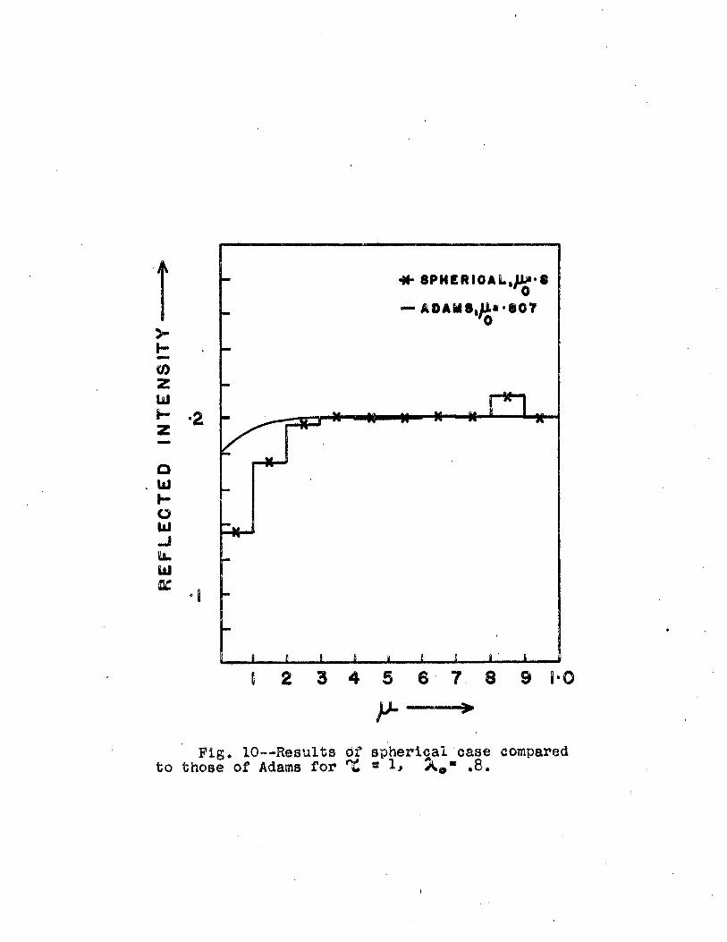
the horizon, and in better agreement towards the zenith. Figure 10 shows the comparison for the case *£ = 1.0 and
JA = 0.80. The agreement is very good for Li between 0.20

38
and 0,80. For smaller the spherical model yields
lower intensities than the plane-parallel case, as expected.
The general agreement between Adams' results and those
of this algorithm are excellent.
Conclusion
The results of the algorithm show excellent agreement
with those of the analogous plane-parallel cases of Coulson et al>
and Adams, which are well substantiated.
On the basis of these comparisons it is concluded that
the spherical model and algorithm developed herein provide
the best representation of the spherical scattering atmosphere
developed to date. This method should have numerous important
applications, and may be extended to explain phenomena occur-
ring in many types of spherical atmospheres.

CHAPTER BIBLIOGRAPHY
1. Adams, Charles, "Solutions of the Equations of Radiative Transfer by an Invariant Imbedding Approach," unpublished master's thesis, Department of Physics, North Texas State University, Denton, Texas, 1968.
2. Coulson, K. L., J. V. Dave, and Z, Sekera, Tables Related to Radiation Emerging from a Planetary Atmosphere with Raylelgh Scattering, Berkeley, University of California Press, 19557
39

APPENDIX
40
41
A T M 0 8 P H E R I 0
THI0KNE88
IEAWTH
Fig. 1—The earth-atmosphere system to eoale

42
• X -
LOOAL SYSTEM
/^PLANET ¥ N
^ SYSTEM
Pig. 2—The coordinate systems
43
I
ATMOSPHERE
INCIDENT
PHOTON
/
Fig. 3—Photon selection

44
©
8ELE0T A
PHOTON
© DETERMINE
© S E L E C T
IP 9T8EE8 YE8^ THE
PLANET
J RHO
COMPUTE
t MAX
COMPUTE INITIAL
PLUX
C O M P U T E
W E I i H T
8 E L E 0 T
RHO
1
.AMBER T
8 E L E 0 T
ANOLE
DETERMINE 80ATTERIN8 TYPE
MIE
SELECT
AN8LE
DETERMINE NEW DIRECTION COSINES
RAYLEISH
YES DETERMINE IP IT 8EES
THE PLANET
COMPUTE t TO RIM A PLUX
OOMPUTE INTENSITY
SELECT
ANSLE
Pig. 4—Flowchart of the scattering simulation

45
I • 0 6 -> s~ '05
co z Ul I- ' 0 4
a uj *03
o UJ -J n- ,Q2 UJ
•Oi
— 0 0 U L 8 0 N i \ Pg « \ • SPHERICAL
— 0 0 U L 8 0 N
\\ •E-IPHERIOAL
\ Q
IJL**4 ' 0
A -
J- L J L
2 3 .4 »5 -6 •? -8 -9 10
JJL >
Pig. 5—Results of spherical oase compared to those of Coulson et al for X *"

46
t CO z til h-
Q su H O til
I&. til ac
•2 h
8PHERI0AL,JlP>»
— 00UL80N,U».« */©
* 8PHERiOAL^JL»*4
OOULSOIMJM*4 *0
J JL J L
'Z "3 *4 • 5 *6 »7 • 8 °9 1*0 • — • >
Fig. 6—Results of spherical case oompared to those of Coulson et al for T " 1* X 9 0.

47
I >-I-
(0 z fijj H Z
o m H o HI -I II. Ill
•flbcaeslte r - U _
8PHCRICAL,jl«*i
— 00UL8OM,U**9 'O
•#§* 8PHEfllOALtJ^*4
-- 00ULS0N,ll««4 0
Pig. 7—Results of spherical case compared to those of Coulson efe al for " 1* % 0
m .8.

•06
1 >
t •05 CO z III i - •04 z
a 1*1 ' 0 3 o Li -J 1*. yj •02 a:
•01 - # •
8PHERI0AL,UL«*S 'O
— OOUL8ON|U«a0 'O
-*• 8PHERI0AL^-4
Q0UL80N,p-4
' » 8 fi I I t i •I °2 -3 -4 -5 -6 -7 -8 -9 1 0
j i >
Pig. 8—Results of cumulative Rayleigh case compared to those of Coulson et al for s . 1 , ° <

I > I-
*© z III H z
a ui H o yi -§
ii. ui a:
•#*8PHCRI0AL|li**f '0
— ADAM9«|l«»t07
I I I ii i t
I 2 3 -4 -5 -6 T -8 -9 1*0
Pig. 9—Results of spherical case compared to those of Adams for t * 1, " 0.
> t CO
liJ I—
Q til
i— o UJ _J u. yj
§c
* 8PHERI0Al,JLU*8
— ADAM8|1L* *807 'o
M % i M
r r - m
, m K
i e i i _L L
I 2 3 4 5 6 7 8 9 80 p- >
Pig. 10—Results of spherical case compared to those of Adams for *X " 1* A # " ,8.
BIBLIOGRAPHY
Books
Cashwell, E. D. and C. J. Everett, Practical Manual on the ' Monte Carlo Method for Random Walk Problems, New York, Pergamon Press, Inc., 1959.
Chandrasekhar, S., Radiative Transfer, New York, Dover Publications, Inc., I960.
Coulson, K.L., J. V. Dave, and Z. Sekera, Tables Related to Radiation Emerging from a PI ane t ary At mo s'phe r e w ft h Raylelgh Scattering, Berkeley, University of California Press, I960.
Hammersley, J. M. and D. C. Handscomb, Monte Carlo Methods, New York, John Wiley and Sons, Inc., 196^
Articles
Kattawar, G. W. and G. N. Plass, "Electromagnetic Scattering from Absorbing Spheres," Applied Optics, VI (August, 1967)# 1377-1382.
Kattawar, G. W. and G. N. Plass, "Resonance Scattering from Absorbing Spheres," Applied Optics, VI (September, 1967)> 15119-1555.
Marchuk, G. I. and G. A. Mlkhailov, "Results of the Solution of Certain Problems of Atmospheric Optics by the Monte Carlo Method," Izv., Atmospheric and Oceanic Physics, III (1967). 227-231.
Marohuk, G. I. and G. A. Mlkhailov, "The Solution of Problems of Atmospheric Optics by a Monte Carlo Method," Izv., Atmospheric and Oceanic Physics, III (1967)? 147-155.
Plass, C-. N. and G. W. Kattawar, "Influence of Single Scattering Albedo on Refleoted and Transmitted Light from Clouds," Applied Optica, VII (February, 1968), 361-367.
51

52
Plass, G. N, and G. W. Kattawar, "Monte Carlo Calculations of Light Scattering from Clouds," Applied Optics. VII (March, 1968); 415-419.
Plass, G. N. and G. W. Kattawar, "Radiant Intensity of Light 6o9t?o5ed f r° m c l o u d s>" Applied Optics, VII (April, 1 9 6 8 ) ,
Smoktii, 0. I., "Multiple Scattering of Light in a Homogeneous Spherically Symmetrical Planetary Atmosphere," Izv., Atmospheric and Oceanic Physics, III ( 1 9 6 7 ) , HO-146.
Reports
Collins, D. G. and M. B, Wells, Monte Carlo Codes for Study 21 Light Transport in the Atmosphere, VoIi7"l"and"TT^ Port Worth, Radiation Research Associates, Inc., 1965 .
Unpublished Materials
Adams, Charles, "Solutions of the Equations of Radiative Transfer by an Invariant Imbedding Approach," unpublished master's thesis, Department of Physics, North Texas State University. Denton, Texas, 1968 .
Private Communications
Mateer, C. L., Laboratory of Atmospheric Sciences, Boulder, Colorado, letter, March, 1968 .