Montana Water Center Annual Technical Report FY … · Montana Water Center Annual Technical Report...
263
Montana Water Center Annual Technical Report FY 2008 Montana Water Center Annual Technical Report FY 2008 1
Transcript of Montana Water Center Annual Technical Report FY … · Montana Water Center Annual Technical Report...

Montana Water CenterAnnual Technical Report
FY 2008
Montana Water Center Annual Technical Report FY 2008 1

Introduction
The Montana University System Water Center is located at Montana State University in Bozeman, wasestablished by the Water Resources Research Act of 1964. Each year, the Center's Director at Montana StateUniversity works with the Associate Directors from the University of Montana - Missoula and Montana Tech- Butte to coordinate statewide water research and information transfer activities. This is all in keeping withthe Center's mission to investigate and resolve Montana's water problems by sponsoring research, fosteringeducation of future water professionals and providing outreach to water professionals, water users andcommunities. To help guide its water research and information transfer programs, the Montana Water Centerseeks advice from an advisory council to help set research priorities. During the 2007/2008 research year, theMontana Water Research Advisory Council members were:
Gretchen Rupp, Director and Steve Guettermann, Assistant Director for Outreach, Montana Water Center
Marvin Miller, Montana Bureau of Mines &Geology and MWC Associate Director
Don Potts, University of Montana and MWC Associate Director
Mark Aagenes, Montana Trout Unlimited, Conservation Director
Jeff Tiberi, Montana Association of Conservation Districts, Executive Director
J. P. Pomnichowski, Montana State Legislator
Daniel Sullivan, Montana Department of Agriculture, Technical Services Bureau Chief
Tyler Trevor, Montana University System, Associate Commissioner
Mike Volesky, Montana Governor's Office, Natural Resources Policy Advisor
Larry Dolan, Hydrologist - Montana Department of Natural Resources and Conservation
Hal Harper, Chief Policy Advisory - Governor's Office
John Kilpatrick, Director - Montana Water Science Center; U.S. Geological Survey
Glenn Phillips, Fisheries Division - Montana Fish, Wildlife & Parks
Richard Opper, Director - Montana Department of Environmental Quality
Introduction 1

Research Program Introduction
Through its USGS funding, the Montana Water Center partially funded three new water research projects andcontinued funding for five other projects for faculty at three of Montana's state university campuses. TheMontana Water Center requires that each faculty research project directly involve students in the field and/orwith data analysis and presentations. This USGS funding also provided research fellowships to three studentsinvolved with water science and aquatic habitat research. Here is an introduction to their work, with thesecond year research projects listed first.
Dr. Chris Gammons of Montana Tech and his team, studied "Temporal and spatial changes in theconcentration and isotopic composition of nitrate in the Upper Silver bow Creek drainage, Montana: Year 2."The project received $6,800. Gammons' graduate student Beverly Plumb presented this work in her master'sdissertation.
Dr. Joel Harper of the University of Montana received $8,941 for his project titled "Historical and futurestreamflow related to small mountain glaciers in the Glacier Park Region, Montana." Considerable progresswas made to use data garnered through field work and incorporate it into computer modeling.
Dr. Clayton Marlow and graduate student Richard Labbe, received $2,000 for their work titled "Sediment andheavy metal source determination and reduction at a reclaimed abandoned mine site, Alta Mine, JeffersonCounty, Montana." Labbe presented the final results in his dissertation at Montana State University during the2008 spring semester.
Dr. Lucy Marshall of Montana State University, received $17,000 for her study of "Predictive modeling ofsnowmelt dynamics: thresholds and the hydrologic regime of the Tenderfoot Creek Experimental Forest,Montana." Work has focused on the development of conceptual snowmelt/hydrologic models.
Dr. Steve Parker, Montana Tech, received $8,585 for his research project: "Carbon cycling and the temporalvariability in the concentration and stable carbon isotope composition of dissolved inorganic and organiccarbon in streams." This work has been key with getting a team of student field researchers involved in datacollection and analysis of specific diel cycles.
Dr. Winsor Lowe of the University of Montana and his team was awarded $6,930 for studying "TheImportance of Ecologically Connected Streams to the Biological Diversity of Watersheds: a case study in theSt. Regis River subbasin, Montana." This project promises to have impact in how the state will address itsobligations under the national Clean Water Act.
Denine Schmitz of Montana State University's Department of Land Resources and Environmental Sciencesreceived $17,000 for research of "Modeling the Potential for Transport of Contaminated Sediment from aMine-Impacted Wetland." Dr. Joel Cahoon assumed responsibility for the project when Schmitz and familyassumed new job responsibilities out of state.
Dr. Andrew Wilcox in the Department of Geosciences at the University of Montana is capitalizing on the rareopportunity to study river channel changes following the removal of a 100 year old hydroelectric dam with hisproject "Evolution of channel morphology and aquatic habitat in the Middle Clark Fork River followingremoval of Milltown Dam." Wilcox was funded $15,818.00.
Student Research Fellows The Water Center's Student Water Research Fellowship Program awarded researchgrants to three Montana University System graduate students. Each showed competence in studying a waterresource problem that is impacting water quality or an aquatic species. They are:
Research Program Introduction
Research Program Introduction 1

Matt Corsi, a Fish and Wildlife doctoral student at the University of Montana received $3,000 for his study of"The Consequences of Introgressive Hybridization: Implications for Westslope Cutthroat TroutConservation."
Sabrina Behnke of Montana State University's Center for Biofilm Engineering received $1,000 for herdrinking water quality work to determine how susceptible detached biofilm particles are to chlorinedisinfection. Sabrina is continuing her work as a doctoral student.
Tyler Smith, a Master's student in MSU's Civil Engineering Department received $1,000 for his work,"Predictive Modeling of Snowmelt and the Hydrologic Response: Tenderfoot Creek Experimental Forest,MT." An outcome of this project was the development of a piece of hydrologic modeling software calledS.P.L.A.S.H. Tyler is also continuing his studies as a doctoral student.
Research Program Introduction
Research Program Introduction 2

Carbon cycling and the temporal variability in theconcentration and stable carbon isotope composition ofdissolved inorganic and organic carbon in streams
Basic Information
Title: Carbon cycling and the temporal variability in the concentration and stable carbonisotope composition of dissolved inorganic and organic carbon in streams
Project Number: 2006MT89BStart Date: 3/1/2006End Date: 9/1/2009
Funding Source: 104BCongressional
District: At large
ResearchCategory: Climate and Hydrologic Processes
Focus Category: Geochemical Processes, Hydrogeochemistry, Water QualityDescriptors:
PrincipalInvestigators: Stephen Parker, Douglas Cameron
Publication
Carbon cycling and the temporal variability in the concentration and stable carbon isotope composition of dissolved inorganic and organic carbon in streams
Carbon cycling and the temporal variability in the concentration and stable carbon isotope composition of dissolved inorganic and organic carbon in streams1

ORI GIN AL PA PER
Temporal Variability in the Concentration and StableCarbon Isotope Composition of Dissolved Inorganicand Organic Carbon in Two Montana, USA Rivers
Stephen R. Parker Æ Simon R. Poulson Æ M. Garrett Smith ÆCharmaine L. Weyer Æ Kenneth M. Bates
Received: 27 February 2009 / Accepted: 30 July 2009� Springer Science+Business Media B.V. 2009
Abstract Here we report diel (24 h) and seasonal differences in the concentration and
stable carbon isotope composition of dissolved inorganic (DIC) and organic carbon (DOC)
in the Clark Fork (CFR) and Big Hole (BHR) Rivers of southwestern Montana, USA. In
the CFR, DIC concentration decreased during the daytime and increased at night while
DOC showed an inverse temporal relationship; increasing in the daytime most likely due to
release of organic photosynthates and decreasing overnight due to heterotrophic con-
sumption. The stable isotope composition of DIC (d13C-DIC) became enriched during the
day and depleted over night and the d13C-DOC displayed the inverse temporal pattern.
Additionally, the night time molar rate of decrease in the concentration of DOC was up to
two orders of magnitude smaller than the rate of increase in the concentration of DIC
indicating that oxidation of DOC was responsible for only a small part of the increase in
inorganic carbon. In the BHR, in two successive years (late summer 2006 & 2007), the
DIC displayed little diel concentration change, however, the d13C-DIC did show a more
typical diel pattern characteristic of the influences of photosynthesis and respiration
indicating that the isotopic composition of DIC can change while the concentration stays
relatively constant. During 2006, a sharp night time increase in DOC was measured;
opposite to the result observed in the CFR and may be related to the night time increase in
flow and pH also observed in that year. This night time increase in DOC, flow, and pH was
not observed 1 year later at approximately the same time of year. An in-stream mesocosm
chamber used during 2006 showed that the night time increase in pH and DOC did not
occur in water that was isolated from upstream or hyporheic contributions. This result
suggests that a ‘‘pulse’’ of high DOC and pH water was advected to the sampling site in the
BHR in 2006 and a model is proposed to explain this temporal pattern.
S. R. Parker (&) � M. G. Smith � C. L. Weyer � K. M. BatesDepartment of Chemistry and Geochemistry, Montana Tech of The University of Montana,1300 W. Park St., Butte, MT 59701, USAe-mail: [email protected]
S. R. PoulsonDepartment of Geological Sciences and Engineering, University of Nevada-Reno, 1664 N. Virginia St.,Reno, NV 89557-0138, USA
123
Aquat GeochemDOI 10.1007/s10498-009-9068-1
Keywords Dissolved organic carbon � Carbon isotopes � Dissolved inorganic carbon �Diel
1 Introduction
Investigations over the past 20 years have shown that diel (24 h) changes in the con-
centration of chemical species in flowing systems are reproducible processes that play an
integral role in the health and water quality of river systems. Healthy rivers can exhibit
large diel pH, dissolved O2 (DO), and CO2 cycles that are largely driven by aquatic
plants and microbes which alternately consume or produce CO2 depending on whether
photosynthesis or respiration is the dominant process (Odum 1956; Pogue and Anderson
1994; Nagorski et al. 2003; Parker et al. 2005, 2007a). These short term variations are
driven by the daily photoperiod, which influences: aquatic photoautotrophs; instream
temperature cycles; changes in dissolved gas gradients between air and water; and affect
either directly or indirectly concentration changes in metals and metalloids (e.g., Nimick
et al. 2003, 2005; Jones et al. 2004; Gammons et al. 2005; Parker et al. 2007a, b and
references therein). While researchers investigating the mechanisms influencing diel
processes have provided great insight into the ‘‘driving forces’’ behind these daily
changes, there is still much that is not well understood. By gaining deeper insight into the
underlying mechanisms controlling diel concentration changes of important dissolved and
particulate species we will be able to develop a better fundamental understanding of how
streams function. This knowledge will help scientists, resource managers and others make
better predictions on how streams will respond to shifting conditions caused by climate
change, changing agricultural practices, restoration activities, nutrient fluxes and
development.
Previous work has demonstrated that there is a significant and reproducible diel cycle
in the stable isotope composition of dissolved inorganic carbon (d13C-DIC) in both the
Clark Fork River (CFR) and Big Hole River (BHR) in Montana, USA as well as a
substantial cycle in the 18O composition of dissolved molecular oxygen (d18O-DO) in the
BHR and other streams (Parker et al. 2005, 2007a, 2009). These daily changes in the
isotope composition of the DIC and DO are caused by the combined effects of photo-
synthesis and respiration of aquatic plants and microbes as well as gas-exchange and
groundwater influx. Additionally, d13C-DIC has been used as a tracer of the origins and
sources of carbon in watersheds (e.g., Gaiero et al. 2005), but these data must be used
carefully since substantial diel changes in d13C-DIC can occur (up to 4.5%, Parker et al.
2009).
Dissolved organic carbon (DOC) represents a significant pool of reduced carbon in most
aquatic ecosystems that is readily available to heterotrophic microorganisms as an energy
source (McKnight et al. 1997; Volk et al. 1997). It has also been suggested that the DOC
pool may be the largest source of carbon for microbial activity (Kaplan and Bott 1982;
Hobbie 1992). Additionally, it has been shown that different size classes of DOC mole-
cules exist and that the distribution can change over a diel period (Amon and Benner 1996;
Zeigler and Fogel 2003). Depending on the size and composition of the DOC some classes
of molecules may be more refractory than others and consequently consumed at different
rates (Thurman 1985; Zeigler and Fogel 2003).
The types and concentration of the DOC can have a significant influence on the chemical
composition of surface waters such as the bioavailability of metal ions and the absorption of
Aquat Geochem
123
light in the visible and UV ranges (McKnight et al. 1997). Much of the literature examining
DOC in rivers has concentrated on sources of organic carbon and its fate and transport to
downstream areas (e.g., Thurman 1985; Olivie-Lanquet et al. 2001; Bianchi et al. 2004,
2007; Hood et al. 2005; Dalzell et al. 2007). Several researchers have shown that diel
changes in DOC concentration occur in streams and can be attributed to daily changes in the
level of productivity of algal communities (e.g., Manny and Wetzel 1973; Kaplan and Bott
1982; Harrison et al. 2005; Spencer et al. 2007). However, there is little literature that
reports investigations of temporal changes in DOC and the 13C-composition of DOC (d13C-
DOC) simultaneously on a diel scale in surface waters (Zeigler and Fogel 2003). Since
community respiration is using the DOC as a carbon source and other aquatic species are
producing organic molecules as a consequence of their daily productivity, it is reasonable to
expect changes in the isotopic composition of the DOC as it is influenced by the daily
changes in the rates of metabolic activity (Barth and Veizer 1999; Zeigler and Fogel 2003;
Zeigler and Brisco 2004).
DOC can include water soluble forms of amino acids, carbohydrates, organic acids,
alcohols as well as fulvic and humic acids (Thurman 1985). Sources of DOC in streams can
include decomposition of detrital organic matter, importation of organics from external
(allochothonous) sources and in-stream production by aquatic plants and microbes
(autochthonous). Microbes using DOC as a carbon source will produce CO2 from respi-
ration with a carbon isotope signature characteristic of the organic carbon substrate (Clark
and Fritz 1997). In temperate regions, plant organic matter, that serves as the carbon source
for microbial respiration has a d13C of -20 to -30% (Clark and Fritz 1997). In contrast,
atmospheric CO2 has d13C of -7 to -8.5% (NOAA 2008) and consequently DIC pro-
duced by gas exchange will be isotopically enriched compared to that produced by
respiration.
A significant portion of DOC in natural waters falls in the category of natural organic
matter (NOM), and most of the NOM fits into the operationally defined subcategories of
fulvic acids (FA) and humic acids (HA; Thurman 1985; Macalady 1998). The fulvic and
humic acids as well as other organic acids are well known for their ability to complex
metal ions in solution (Saar and Weber 1982; Clapp et al. 1998). It is known that the fulvic
and humic acids can contribute to daily variations in surface water iron concentrations by
affecting Fe redox cycling through changes in the photoreactivity of Fe in the aqueous
system (Voelker et al. 1997; Hrncir and McKnight 1998).
In this study, we investigated diel changes in the concentration of DOC and DIC in two
different rivers systems (CFR and BHR). These rivers are geographically close but
exhibited approximately inverse diel patterns in the concentration of DOC during the late
summer of 2006. An in-stream mesocosm chamber was used in the BHR during 2006 to
compare diel cycles and levels of DOC and DIC that were isolated from the flowing water
column or hyporheic water exchanges. A follow-up study was conducted in the BHR
1 year later to assess the reproducibility of the diel DOC pattern observed the previous
year. Additionally, in order to identify possible sources of DOC in the BHR a series of
seeps (streamside springs) and shallow sediment water was sampled during the follow-up
work in 2007. The rates of DOC consumption and DIC production in the CFR were
compared in order to determine what portion of the inorganic carbon being produced
resulted from the oxidation of DOC. The d13C-DOC was examined in the CFR as well as
the d13C-DIC in the CFR and BHR. These isotope results are used here in conjunction with
the seep and chamber data to investigate the relationship of the diel changes in DOC and
DIC to the processes influencing these changes. Models are presented to help interpret the
Aquat Geochem
123
diel behavior of DOC in the CFR and the differences in the diel behavior of DOC observed
in the BHR between 2006 and 2007.
2 Field Sites
2.1 CFR Site
The field site on the Clark Fork River (46�2305100N; 112�4403300W; sampling site CFRG)
was within the city limits of Deer Lodge, MT and directly across from the USGS gaging
station (Fig. 1, USGS Gage #12324200, 1,372 m elevation). Streamflow measurements
were taken from the USGS gaging station which records every 15 min. The Clark Fork
here is a second order stream with a discharge of roughly 0.6–60 m3 s-1 depending on the
time of year. The river in the study reach has moderate alkalinity (*3,200–3,700 leq l-1;
Parker et al. 2007a) and a pH range of about 8.0–9.0 during the summer months. Aquatic
plants are dominated by Cladophora and diatom algae (Watson 1989). The mining and
smelting centers of Butte and Anaconda are situated at the headwaters of the upper Clark
Fork River along Silver Bow and Warm Springs Creeks, respectively (Fig. 1) such that the
floodplain and streambed of the upper Clark Fork River contain highly elevated quantities
of metals and metalloids (e.g., Fe, Cu, Zn, Pb, Cd, As) deposited as the result of mining,
milling, and smelting activities (Moore and Luoma 1990). Currently, most of the heavy
metal load in Silver Bow Creek is removed by a lime treatment facility at Warm Springs
(Fig. 1). However, elevated concentrations of dissolved arsenic have been measured in the
water exiting the treatment ponds ([40 lg L-1) during summer base-flow periods (Duff
2001; Gammons et al. 2007). Diel changes in the concentration of metals and arsenic in the
upper CFR have been previously characterized (Brick and Moore 1996; Parker et al.
2007a; Gammons et al. 2007).
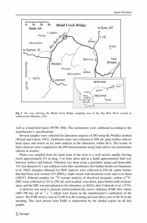
2.2 BHR Site
The field site near the Mudd Creek Bridge on the Big Hole River (45�4802800N,
113�1805100W; sampling site BHRG) was about 50 m upstream from the USGS gaging
station (Fig. 2; USGS Gage #6024540, 1795 m). Annual flows range from 5 to 140 m3 s-1
depending on time of year. Flow data for this site was obtained from the USGS gaging
station which records discharge every 15 min. The BHR is a headwater tributary to the
Missouri River and is a free-flowing river draining a sparsely-populated, high elevation
basin (*1,900 m above sea level) of approximately 7,200 km2 in extent. This river is
relatively pristine and there is little historical impact from mining or industrial sources. The
principal activities in the basin are agriculture and recreation.
Previous work (Gammons et al. 2001; Ridenour 2002; Wenz 2003; Parker et al. 2005)
has summarized the general geochemical characteristics of the Big Hole River. Overall, the
Big Hole River at Mudd Creek Bridge can be classified as a Na–Ca-bicarbonate water, with
alkaline pH and low to moderate alkalinity (1,500–1,800 leq L-1). The lower alkalinity of
the BHR versus the CFR described above results in lower buffering capacity of the BHR
stream water that often leads to larger ranges in and higher absolute values of pH during
summer low flow periods.
Aquat Geochem
123

3 Methods
3.1 Field Methods
3.1.1 Clark Fork River
Diel sample collection on the CFR began on 27 July 2006 at 11:15 and continued until
13:15 on 28th of July. All times are reported as local time (MDT, GMT—0600).
In situ temperature, pH, specific conductivity (SC), dissolved oxygen (DO) concen-
tration and percent O2 saturation were measured at each sampling time with a Hydrolab
MS-5 datasonde (Luminescent DO probe) or an In Situ Troll 9000 (Clark DO probe) as
State of Montana
Butte
State of Montana
ButteDeer Lodge
Anaconda Warm Springs Treatment Ponds
Clark Fork River
Warm Springs Creek
Willow Creek
Mill Creek
Treatment Ponds
Washoe Smelter
I-90
Opportunity Tailings Ponds
Butte
Silver Bow Creek
Creek
10 km
USGS
CFRG site
Deer Lodge
Gaging Station
Clark Fork
140
ClarkRiver
I-90
1450
00
Scale: 1 km
112° 45‘
46° 22.5‘
N
Fig. 1 Location map of theupper Clark Fork River showingButte, MT; Anaconda, MT;Warms Springs Ponds,Opportunity Ponds and the CFRGsampling site on the Clark ForkRiver near Deer Lodge, Montana,USA
Aquat Geochem
123
well as a hand-held meter (WTW 340i). The instruments were calibrated according to the
manufacturer’s specifications.
Several samples were collected for laboratory analysis of DO using the Winkler method
(Wetzel and Likens 1991). Unfiltered water was collected in 500 mL glass bottles with no
head space and stored on ice until analysis in the laboratory within 48 h. The results of
these analyses were compared to the DO measurements using hand and in situ instruments
(shown in results).
Water was sampled from the main stem of the river in a well mixed, rapidly flowing
reach approximately 0.5 m deep, 3 m from shore and at a depth approximately half way
between surface and bottom. Filtration was done using a peristaltic pump and disposable
142 mm diameter 0.1 lm cellulose-ester filter membranes (for further details see Gammons
et al. 2005). Samples (filtered) for DOC analysis were collected in 250 mL amber bottles
that had been acid washed (5% HNO3), triple rinsed with deionized water and oven dried
(100�C). Filtered samples for 13C-isotope analysis of dissolved inorganic carbon (d13C-
DIC) were collected in 125 or 250 mL acid-washed, oven dried, glass bottles with no head-
space and the DIC was precipitated in the laboratory as SrCO3 after Usdowski et al. (1979).
A detector was used to measure photosynthetically active radiation (PAR) flux values
(400–700 nm, lE m-2 s-1) which were based on the manufacturer’s calibration of the
sensor. The PAR went to zero at 21:00 h in the evening and rose above zero at 06:30 in the
morning. This dark period (zero PAR) is represented by the shaded region on all diel
graphs.
Mudd Creek Bridge
River
I-15
Hol
e
to Butte, MT
2876m
2844mPintler
Mountains
Scale, km0 10 3020
Scale, km0 10 3020
Wisdom
Twin Bridges
Melrose
BigH
to Salmon, ID3105m
B
Mountains
Wisdom
Jackson
g
3400m
3237m
eaverhead R
a
Pioneer
Mountains
MONTANAange
Missouri
River
Billings
Helena
Butte Map Detail
Fig. 2 Site map showing the Mudd Creek Bridge sampling area of the Big Hole River located insouthwestern Montana, USA
Aquat Geochem
123

All samples collected in the field were stored on ice, in sealed plastic bags and returned
to the laboratory immediately following the field work.
3.1.2 Big Hole River
Two separate diel samplings occurred on the BHR approximately 1 year apart: 8 to 9
August 2006 and 31 July to 1 Aug 2007. Sampling was performed similar to that described
in the previous section on the Clark Fork site. Alkalinity was measured in the field using a
Hach titrator and standardized H2SO4. Samples from seeps above the main sampling site
were collected with a clean 60 mL syringe that was triple rinsed with sample water and
then filtered using 0.2 lm PES syringe filters into glass bottles. Sediment pore water was
collected at two locations near the sampling site with a 60 mL syringe that was inserted
approximately 12 cm into the shallow sediments in the middle of the river. The syringe
plunger was very slowly withdrawn to minimize water from being pulled around the barrel
of the syringe from the above river; taking 2–3 min to fill the 60 mL volume. This water
was filtered using 0.2 lm PES filters into glass bottles.
An isolation chamber was used during the 2006 sampling that was made from a 10 cm
inside diameter clear acrylic plastic cylinder 22 cm long. One end was sealed and the other
end was removable (both clear acrylic). Each end had a tubing connector fastened to a
drilled and threaded hole in the center. Prior to the start of the diel sampling, the chamber
was filled approximately half-full with cobbles ranging from 2 to 10 cm in diameter
collected from the sampling site that were covered with attached periphyton and biofilms.
The chamber lid was sealed with silicone vacuum grease and held in place with an elastic
strap. Clear plastic tubing was used to connect the chamber to a peristaltic pump mounted
on a tethered platform in the river, then to a low volume flow chamber on a datasonde and
back to the chamber. The chamber and datasonde were placed on the river bottom at a
depth of *0.5 m. At the beginning of the sampling period, the chamber was flushed with
river water, filled and purged to remove most of the trapped air. The chamber water was
sampled every 2 h as described previously for DOC and DIC; then flushed and refilled with
fresh river water. The datasonde connected to the chamber recorded pH, temperature, DO,
and SC every 30 min throughout the diel period.
3.2 Analytical Methods
A pre-concentration step for samples for d13C-DOC analysis was performed by evapo-
rating 250 mL of filtered river water to near-dryness at 50�C and resuspending in 4 mL of
1% H3PO4.
The SrCO3 precipitates (described above) for d13C-DIC and the DOC concentrates for
d13C-DOC were analyzed using a Eurovector elemental analyzer interfaced to a Micromass
Isoprime stable isotope ratio mass spectrometer after Harris et al. (1997) and Gandhi et al.
(2004), respectively. Replicate analyses (three per sample set) indicated an average relative
standard deviation (RSD) of 0.95% for d13C-DOC and 0.55% for d13C-DIC.
All analyses for total carbon (TC) and DOC were performed at Montana Tech using an
Ionics (Model 1505) Total Carbon Analyzer (combustion method). All samples for TC
analysis used filtered, unacidified water. Samples for DOC analysis used filtered water that
was acidified to 1% (v/v) with concentrated H3PO4 and sparged for 5 min with N2. These
samples were then sparged in the instrument for an additional 3 min with CO2-free air and
analyzed. Standards were prepared from a stock solution of 1,000 mg l-1 potassium
hydrogen phthalate (KHP) prior to each analysis. All glassware used for carbon analyses
Aquat Geochem
123

was acid-washed and oven dried prior to use (100�C). DIC was determined by subtracting
DOC concentration from TC. Replicate analyses indicated an RSD of 5% for DOC and
DIC.
3.3 Modeling
The partial pressure of dissolved (wet) CO2 (pCO2, latm) was calculated for the CFR and
BHR with the modeling program CO2SYS (Lewis and Wallace 1998) using the temper-
ature, pH and either the total alkalinity or DIC to determine the carbon speciation.
4 Results and Discussion
4.1 Clark Fork River
4.1.1 Field Results
Temperature, flow, pH, and specific conductivity from the diel sampling on the CFR in
2006 are show in Fig. 3. A diel pH change of approximately 0.6 units (range 7.8–8.4) was
observed which is attributed to daytime net consumption of CO2 by aquatic photosynthesis
and night time production of CO2 by community respiration. The temperature reached a
daytime maximum of 24.6�C and night time minimum of 16.5�C. A diel change in flow of
approximately 13% was observed most likely due to evapo-transpiration in the streamside
riparian zones (Bond et al. 2002). The dissolved oxygen reached a daytime high of 158%
of saturation (385 lmol L-1) and a night time low of 65% (164 lmol L-1). DO con-
centrations (n = 3) determined by Winkler titration were in good agreement with instru-
ment readings (Fig. 3c). The pCO2 was above atmospheric partial pressure (*252 latm)
during the whole diel period; decreasing during the day and increasing at night (Fig. 3c).
4.1.2 DOC and DIC
DOC showed a 1.8-fold diel change in concentration from a minimum of 124 to a max-
imum of 231 lmol C L-1 (Fig. 4a). At the same time the average concentration of DIC
was *52-times higher than that of the DOC. The DIC showed a *5-fold diel change in
concentration from a minimum of 3.4 to a maximum of 17.0 mmol C L-1 (Fig. 4a). The
diel change in DOC is most likely produced by release of soluble organic carbon com-
pounds (i.e., amino acids, sugars, organic acids) by photosynthetic organisms during the
daytime (Kaplan and Bott 1982; Vymazal 1994 and references therein) followed by
consumption of those soluble organics by heterotrophic microbes during the night. The
gradual increase in DOC after about 23:00 suggests a net accumulation due heterotrophic
processing of larger insoluble organics from sediments or particulates (Zeigler and Fogel
2003). The DIC concentration decreased during the daytime due to removal of CO2 by
photosynthesis and increased at night due to community respiration.
The molar ratio of DIC/DOC reached a minimum of 16 at *17:00 and a maximum of
104 at *06:00 the following morning (Fig. 4b). This large increase in DIC relative to
DOC at night suggests that oxidation of DOC contributed only a small part of the increase
in DIC and that the majority of DIC was produced from other sources (e.g., aerobic or
anaerobic respiration of microbes within the sediment bed; or groundwater influx). The
Aquat Geochem
123
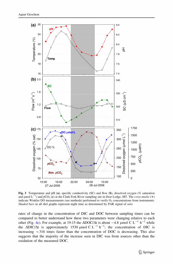
rates of change in the concentration of DIC and DOC between sampling times can be
compared to better understand how these two parameters were changing relative to each
other (Fig. 4c). For example, at 19:15 the DDOC/Dt is about -4.8 lmol C L-1 h-1 while
the DDIC/Dt is approximately 1530 lmol C L-1 h-1; the concentration of DIC is
increasing *316 times faster than the concentration of DOC is decreasing. This also
suggests that the majority of the increase seen in DIC was from sources other than the
oxidation of the measured DOC.
(o C)
24
26
8.2
8.4(a)
(b)
(c)
pH
Tem
pera
ture
(
18
20
22
pH
7.6
7.8
8.0
Temp
16 7.4
1 ) 1.6
2.0
-1)530
540
SC
Flo
w (
m3 s
-
0.8
1.2
SC
(µ S
cm
-
510
520Flow
5 0
n (%
sat
)
150
175
(µm
ol L
-1)
300
350
m)1250
1500
1750
DO %
DO µmol/L
Dis
solv
ed o
xyge
n
75
100
125
Dis
solv
ed o
xyge
n (
150
200
250
pCO
2 (
µ atm
250
500
750
1000DO %
pCO2
Atm pCO2
10:00 16:00 22:00 04:00 10:0050
D
1000
27-Jul-2006 28-Jul-2006
Atm. pCO2
Fig. 3 Temperature and pH (a), specific conductivity (SC) and flow (b), dissolved oxygen (% saturationand lmol L-1) and pCO2 (c) at the Clark Fork River sampling site in Deer Lodge, MT. The cross marks (1)indicate Winkler DO measurements (see methods) performed to verify O2 concentrations from instruments.Shaded bars in all diel graphs represent night time as determined by PAR signal of zero
Aquat Geochem
123

4.1.3 d13C-DOC and d13C-DIC
The isotopic composition of DOC (d13C-DOC) and DIC (d13C-DIC) also showed changes
over the sampling period (Fig. 5). Diel changes in d13C-DIC have been observed previ-
ously in the CFR and BHR (Parker et al. 2005, 2007a). Photosynthesis removes CO2 during
the day with a reported isotopic depletion of about -29% (Falkowski and Raven 1997);
such that the residual DIC becomes isotopically enriched. Gas-exchange with atmospheric
C L
-1)
12
16
20
C L
-1)
200
240DIC (mmol C L-1)
DOC (µmol C L-1)
(a)
DIC
(m
mol
C
4
8
12
DO
C (
µmol
C
160
120
120
DIC/DOC
(b)
DIC
/DO
C
40
80
0
h-1)
0
2000
h-1
)10
20
(c) ∆DIC
∆DIC
/ ∆t (
µmol
L-1
-4000
-2000
0∆D
OC
/∆t (
µmol
L-1
-10
0
10
27-Jul-2006 28-Jul-2006 10:00 16:00 22:00 04:00 10:00
∆
-8000
-6000 ∆
-30
-20∆DOC
Fig. 4 DOC (lmol C L-1) and DIC (mmol C L-1) at CFRG during diel sampling in 2006 (a); molar ratioof DIC to DOC at CFRG (b) and the rate of change in DIC (mmol C L-1 h-1) and DOC (lmol C L-1 h-1)(c). Error bars represent 5% RSD based on replicate determinations
Aquat Geochem
123

CO2 (d13C = -7 to -8.5%) will tend to elevate the d13C-DIC which had an average value
over the diel period of -12.4%. However, as reported in Sect. 4.1.1 the pCO2 was above
atmospheric levels during the diel period such that the net flux of CO2 would have been
from the water to the atmosphere for the 24-h period. Diffusional fractionation associated
with CO2 outgassing should have caused the d13C-DIC to become isotopically heavier but
the opposite was observed, with the d13C-DIC becoming increasingly depleted over night.
This is consistent with community respiration being the dominant process which was
influencing the d13C-DIC.
The d13C-DOC showed the inverse isotopic diel trend to that of the DIC. The con-
centration of DOC increased during the day (Fig. 4a) due to soluble organics that were
‘‘leaking’’ from photosynthetic organisms and since photosynthesis discriminates against13C it follows that the DOC produced during this time will be isotopically depleted. Zeigler
and Fogel (2003) suggested that the daytime decrease in d13C-DOC observed in a tidal
wetland was due to the exudation of carbohydrates produced by phytoplankton and
macrophytes. As photosynthesis decreased in the late afternoon (*17:00), community
respiration consumed this pool of soluble (isotopically light) organics, discriminating
against the heavier isotope (kinetically) such that the remaining DOC pool becomes iso-
topically enriched (concentration decreasing, Fig. 4a). It is also possible that these
‘‘leaking’’, isotopically light photosynthates such as carbohydrates are more readily bio-
available and are used first for respiration (Zeigler and Fogel 2003). After *23:00 the
isotopic composition of the pool stabilizes at approximately -26.9%. The d13C of the
local aquatic and streamside vegetation was not measured during this study, but temperate
region C3 plants should have an isotope composition in the range of -20 to -30% (Clark
and Fritz 1997). Consequently, this d13C-DOC plateau from 01:00 to 09:00 may reflect the
DOC being produced by microbial degradation of detritus with an isotope signature typical
of temperate region vegetation. This is consistent with the increase in DOC concentration
after 23:00 (discussed above) being due to heterotrophic degradation of organic detritus
accumulated within the sediment bed.
-11.0 -26.0
)
12 0
-11.5
)
-26.5
DOCδ13
C-D
IC (
‰
-12.5
-12.0
13C
-DO
C (
‰
-27.0
DIC
δ
-13.5
-13.0
δ1
-27.5
10:00 16:00 22:00 04:00 10:00-28.0
6002-luJ-826002-luJ-72
Fig. 5 d13C-DOC and d13C-DIC values measured during diel sampling in the CFR. Error bars represent aRSD of 0.95% for d13C-DOC and 0.55% for d13C-DIC
Aquat Geochem
123

During the night as community respiration consumes the isotopically light DOC and
insoluble organic matter in the sediments, it produces light CO2 which causes the d13C-
DIC to continue dropping until photosynthesis reverses the trend starting about 06:30
(Parker et al. 2009).
4.2 Big Hole River
4.2.1 Field and Isolation Chamber Results
Diel samplings were conducted on the BHR in two successive years during late summer,
low flow conditions (2006 and 2007) within 8 days of the same date each year (Fig. 6). The
hydrographs for a 6–7-day period bracketing the sampling for the 2 years show that the
average flow in 2007 was about 1.7-times higher than in 2006 during the sampling period
and that different temporal flow patterns were present in the 2 years (Fig. 7). The flow
during the diel sampling period in 2006 showed a *2.7-fold minimum to maximum
increase and exhibited a sharp decrease during the late afternoon (*17:00) followed by a
gradual increase with a maximum at about 01:00–03:00 (Fig. 6b). The flow in 2007
showed a *1.3-fold minimum to maximum increase during the sampling period with a
gradual decrease throughout the afternoon reaching a minimum about 21:00 through 02:00
followed by a gradual increase through the following morning (Fig. 6e). The 2007 pattern
is more typical of one expected to be produced by evapo-transpiration from productive
2006
)
249.2
2007
)
249.2pH Temp
Tem
pera
ture
(o C
)
18
20
22
pH
8.0
8.4
8.8
Tem
pera
ture
(o C
)
18
20
22pH
8.0
8.4
8.8
Temp
Temp
pH
T
14
16
7.6
T
14
16
7.6
2.5
3.0
165
170
2.5
3.0
165
170Flow
Flo
w (
m3 s
-1)
1.5
2.0
2.5
SC
(µ S
cm
-1)
150
155
160
Flo
w (
m3 s
-1)
1.5
2.0
2.5
SC
(µ S
cm
-1)
150
155
160
Flow
SC
SC
1.0145
1.0145
t) 120
150
-1)400
500
m)
3000
t)120
150
-1)400
500
m)
3000DO%
DO%pCO2
DO
(%
sat
60
90
DO
(µm
ol L
100
200
300
pCO
2 (µa
tm
1000
2000
DO
(%
sat
60
90
DO
(µm
ol L
100
200
300
pCO
2 (µa
tm
1000
2000DO µmol/L
DO µmol/LpCO2 Atm. pCO2 Atm pCO
09:00 15:00 21:00 03:00 09:00
300 09:00 15:00 21:00 03:00 09:00
30
100
0
8-Aug-2006 9-Aug-2006 31-Jul-2007 1-Aug-2007
p 2 Atm. pCO2
(a)
(b)
(c) (f)
(e)
(d)
Fig. 6 Temperature and pH (a; 2006) and (d; 2007); flow and specific conductivity (SC) (b; 2006) and (e;2007); and dissolved oxygen (% saturation and lmol L-1) (c; 2006) and (f; 2007) for the BHR. The crossmarks (1) indicate Winkler DO measurements (see methods) performed to verify O2 concentrations frominstruments
Aquat Geochem
123

upstream riparian zones (Bond et al. 2002) while the pattern observed in 2006 is not well
understood (discussed below).
The pH variation observed in 2006 is very unusual with a sharp pH drop in late
afternoon (*17:00), at approximately the same time that the flow dropped (Fig. 6a). This
was followed by a gradual increase in pH with a maximum at *03:00; approximately the
same time that the flow peaked in 2006. The late afternoon decrease in flow in 2006
described above was also accompanied by a sharp increase in specific conductivity (SC) at
the same time (*18:00, Fig. 6b). The SC dropped after this time with a minimum at
*03:00, the same time that the flow reached a maximum. The behavior of DO in 2006 was
‘‘normal’’ with the exception of a small shoulder at approximately 19:00 which corre-
sponds to the sharp flow decrease in the late afternoon (Fig. 6c). In contrast to the CFR
described above, the pCO2 in the BHR in 2006 was below atmospheric levels
(*252 latm) for the 24-h sampling period (Fig. 6c) which is due to the high pH (avg. 9.1)
and high productivity as shown by the large diel change in O2 concentration (37–152%
sat.) during this base flow period. The late afternoon drop in pH described above (*17:00)
was mirrored by a small increase in pCO2 followed by a night time decrease as the pH
began to rise. This is an unusual pCO2 pattern since it usually increases over night due to
community respiration and decreasing pH, as observed in the CFR (Fig. 3c).
In 2007, the changes in flow, SC, and pH were more typical of ‘‘normal’’ stream
behavior (Fig. 6d, e). The diel change in DO was not as large in 2007 as in 2006 and was
possibly modulated by the larger flow (Fig. 6f). Maximum stream temperature was higher
in 2007 than 2006 which also decreased O2 solubility. The pCO2 during 2007 was above
atmospheric levels except for a brief period in the afternoon (*16:00–20:00) and showed a
more ‘‘typical’’ pattern (Fig. 6f). The higher pCO2 levels are in part due to the lower pH
values in 2007 (avg. 8.1) versus 2006 (avg. 9.1).
An isolation chamber with stream water plus cobbles and attached periphyton was used
during the 2006 sampling (Fig. 8a). This allowed a comparison of temperature, pH, and
DO between the river and water in the chamber which was isolated from chemical species
3.5
4.0
2007
10:00Start
11:00End
-1
2 5
3.0
2007F
low
m3
2.0
2.52006
1.0
1.5
Days
0.51 2 3 4 5 6 7
s
Fig. 7 Hydrographs (USGS gage data) for the BHR site for a 6–7 day period around the field work in 2006and 2007. Red lines show the sampling period in both years and dashed lines show the approximate starting(10:00) and ending (11:00) times for sampling
Aquat Geochem
123
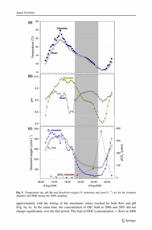
transported to the sampling site from upstream or from hyporheic discharge (Fig. 9).
Consequently, the observed changes in chemistry of the chamber water were dominated by
interactions with the enclosed benthic materials. Temperature and DO both in the chamber
and in the river were similar through the diel period although at night the DO in the
chamber did reach a minimum of about 31 lmol L-1 versus 115 lmol L-1 in the river
(Fig. 9a, c). This night time difference in DO was most likely due to the absence of gas
exchange with the atmosphere in the chamber. The pH in the chamber did not show the
same unusual pattern displayed in the river (Fig. 9b). Since the chamber was refilled with
river water every 2 h, it does show evidence of a subdued version of the decrease in pH
seen in the river at *19:00–20:00. The pH in the water isolated in the chamber showed a
0.13 unit change in pH versus 0.86 units in the river in the time period from 17:00 to 19:00.
Since the pH profile in the chamber was similar to the more typical pattern found in river
systems (i.e., CFR Fig. 3a) and that it was refilled with river water every 2 h emphasizes
the temporal period over which the pH modification can occur. The pCO2 in the chamber
(Fig. 9c), similar to pH, showed a more typical diel behavior and did not show the small
increase around 19:00 as was seen in the river. The potential causes of these differences in
the diel pH and pCO2 patterns in 2006 between the river and the chamber will be discussed
in the next section.
4.2.2 DOC and DIC
A 4.6-fold minimum to maximum diel change in DOC in the BHR was observed in 2006
while no regular diel change in DOC concentration was observed in 2007 (Fig. 10a, b).
The night time peak in DOC concentration in 2006 occurred at *01:00, which coincides
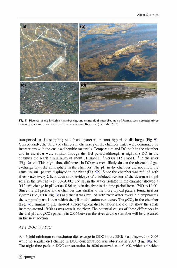
Fig. 8 Pictures of the isolation chamber (a), streaming algal mats (b), area of Ranunculus aquatilis (riverbuttercups, c) and river with algal mats near sampling area (d) in the BHR
Aquat Geochem
123
approximately with the timing of the maximum values reached by both flow and pH
(Fig. 6a, b). At the same time, the concentration of DIC both in 2006 and 2007 did not
change significantly over the diel period. The load of DOC (concentration 9 flow) in 2006
24
26
Chamber
(a)
Tem
pera
ture
(o C
)
18
20
22
River
14
16
9.5
10.0 Chamber(b)
pH
8.5
9.0River
8.0
mol
L-1
)
400
500
450
600O2 chamber
(c)
Dis
solv
ed o
xyge
n (µ
m
100
200
300
pCO
2 (
µ atm
)
150
300
O2 river
6002-guA-96002-guA-8
08:00 13:00 18:00 23:00 04:00 09:00
D 100
0pCO2 chamber
Fig. 9 Temperature (a), pH (b) and dissolved oxygen (% saturation and lmol L-1) (c) for the isolationchamber and BHR during the 2006 sampling
Aquat Geochem
123
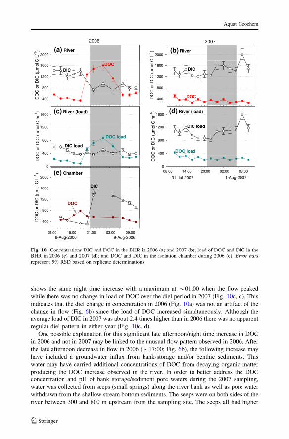
shows the same night time increase with a maximum at *01:00 when the flow peaked
while there was no change in load of DOC over the diel period in 2007 (Fig. 10c, d). This
indicates that the diel change in concentration in 2006 (Fig. 10a) was not an artifact of the
change in flow (Fig. 6b) since the load of DOC increased simultaneously. Although the
average load of DIC in 2007 was about 2.4 times higher than in 2006 there was no apparent
regular diel pattern in either year (Fig. 10c, d).
One possible explanation for this significant late afternoon/night time increase in DOC
in 2006 and not in 2007 may be linked to the unusual flow pattern observed in 2006. After
the late afternoon decrease in flow in 2006 (*17:00; Fig. 6b), the following increase may
have included a groundwater influx from bank-storage and/or benthic sediments. This
water may have carried additional concentrations of DOC from decaying organic matter
producing the DOC increase observed in the river. In order to better address the DOC
concentration and pH of bank storage/sediment pore waters during the 2007 sampling,
water was collected from seeps (small springs) along the river bank as well as pore water
withdrawn from the shallow stream bottom sediments. The seeps were on both sides of the
river between 300 and 800 m upstream from the sampling site. The seeps all had higher
2006C
L-1
)
2000
2007
C L
-1)
2000(a) River (b) River
C o
r D
IC (
µmol
C
800
1200
1600
C o
r D
IC (
µmol
C
800
1200
1600DOCDIC DIC
DO
C
400 DO
C
400
C h
r-1)
1600(c) River (load)
C h
r-1)
1600(d) River (load)
DOC
OC
or
DIC
(µm
ol
400
800
1200
OC
or
DIC
(µm
ol
400
800
1200
DIC load
DOC load
DOC load
DIC load
DO
0 08:00 14:00 20:00 02:00 08:00
DO
0
31-Jul-2007 1-Aug-2007
ol C
L-1
)
1600
2000(e) Chamber
DIC
DOC
OC
or
DIC
(µm
o
800
1200
1600 DIC
8-Aug-2006 9-Aug-2006 09:00 15:00 21:00 03:00 09:00
D 400
Fig. 10 Concentrations DIC and DOC in the BHR in 2006 (a) and 2007 (b); load of DOC and DIC in theBHR in 2006 (c) and 2007 (d); and DOC and DIC in the isolation chamber during 2006 (e). Error barsrepresent 5% RSD based on replicate determinations
Aquat Geochem
123

DOC concentrations and lower pH values than the river water at the sampling site (Fig. 11;
Table 1). The average DOC concentration of the seeps was 1,385 lmol C L-1 while the
average DOC in the river over the diel period was 341 lmol C L-1. The DOC concen-
tration of the shallow sediment water sampled was similar to that of the river (Fig. 11),
which is characteristic of shallow, short range hyporheic flow paths (Poole et al. 2008). The
average pH of the seep waters was 6.8 while the average pH of the river during the 2007
diel sampling was 8.1 (9.1 in 2006). This suggests that if the night time increase in DOC in
2006 was due to a significant influx of bank storage water, then the pH should have
decreased simultaneously; not increased. This is not to suggest that streamside/ground-
water contributions of DOC and other solutes did not occur but that those contributions
were relatively constant while the large night time increase in DOC was produced by a
separate process.
Another hypothesis that has been considered to explain the large diel changes in flow
that have been observed periodically during late summer in the BHR has been the presence
of large stretches of algae and macrophytes (Ranunculus aquatilis and other species) that
float to the surface during the day while they are actively photosynthesizing, effectively
forming an ‘‘in-stream’’ dam (see Fig. 8b–d). At night these photosynthetic organisms sink
toward the bottom allowing the trapped water to flow down the river as a wave. This model
is consistent with stream flow observations in this reach of the river during a similar flow
regime in 2005 when the river stage (water level) increased and the flow decreased (C.
Gammons personal communication). This might explain the decrease in flow in the late
afternoon during 2006 followed by an increase in water at night from upstream as the in-
stream damming action ceased. This pulse of water that was retarded by the plants and
algae during the day may have been higher in pH due to photosynthetic removal of CO2
and contain higher amounts of DOC due to leakage of organic photosynthates as discussed
above in Sect. 4.1.2.
This model that conceptualizes a ‘‘wave’’ of water moving down the river can be further
analyzed by looking at the SC of the water over the diel period. The average diel SC of the
river was significantly lower in 2006 (157 lS cm-1 ± 6.7; n = 51) than that of the seeps
L-1)
2500
3000
SeepsO
C (
µ mol
C L
1500
2000
DO
500
1000
River
Seds
10:00 16:00 22:00 04:00 10:000
31-Jul-2007 1-Aug-2007
Fig. 11 Concentration of DOC (lmol C L-1) in seeps (red), shallow sediments (green) and the BHR (opentriangles) during the 2007 sampling site
Aquat Geochem
123

sampled in 2007 (avg. 329 lS cm-1; range: 124–622). Additionally, the effect of the
higher SC of the seeps on the river SC was investigated with a synoptic survey through the
sampling area in 2007. This survey showed consistently higher conductivity water near
the stream banks (avg. 157 ± 4.6 lS cm-1, n = 8) than in the middle of the channel (avg.
147 ± 3.9 lS cm-1, n = 49) which shows that additions of water from streamside areas
were entering the river. Assuming that the chemistry of the seep/groundwater was similar
in the 2 years, the increase in SC of the river observed in 2006 (Fig. 6b) during the late
afternoon when the flow decreased is consistent with a lower volume of river water (lower
SC) relative to groundwater (higher SC). This was then followed by a decrease in SC as the
flow increased in the first part of the night (*21:00–01:00; Fig. 6b) possibly related to an
increase in the volume of river water being advected into the sampling area relative to the
groundwater contributions.
In further support of this model, the DOC concentration and pH in the isolation chamber
did not display the same night time increase observed in the river in 2006 (Fig. 10e). This
difference in DOC and pH behavior between the chamber and the river is consistent with
the model described above suggesting that a ‘‘slug’’ of water migrated downstream that
was higher in pH; passing the BHR sampling site between 17:00 and 01:00. If the increase
in DOC and pH was produced by aquatic vegetation in the direct area of the sampling site,
it should have been observed at some level in the chamber as well as in the river. Addi-
tionally, the DIC concentration in the chamber showed a pattern that is more ‘‘typical’’ of
productive systems with the DIC decreasing during the day, while photosynthesis is the
dominant metabolic process, resulting in a net removal of CO2; followed by increasing
CO2 at night as community respiration returns it to the water column (Fig. 10e). This was
the same pattern observed for the DIC concentration in the CFR (Fig. 4a).
Another possible cause of the large and reproducible abnormal flow cycle observed in
2006 could have been a significant daily change in irrigation withdrawals upstream from
Table 1 Concentrations of DOC from seeps and sediments from the Big Hole River sampled during 2007
Site T (�C) pH SC DO % sat DO lmol/L DOC lmol C/L Location
Seep 1a 20.8 6.76 130 75.2 165 1,252 N 45�48.4290; W 113�19.1470
Seep 1b NA NA NA NA NA 1,442 N 45�48.4290; W 113�19.1470
Seep 2a 25.2 6.88 129 105.2 206 1,155 N 45�48.4330; W 113�19.1640
Seep 2b NA NA NA NA NA 963 N 45�48.4330; W 113�19.1640
Seep 3 19.5 6.23 157 52.0 117 770 N 45�48.4330; W 113�19.1740
Seep 4 23.0 7.12 157 135.5 288 1,252 N 45�48.4360; W 113�19.1950
Seep 5a 20.1 6.91 622 0.9 2.0 1,536 N 45�48.7080; W 113�19.5640
Seep 5b 11.7 7.05 608 43.9 119 1,252 N 45�48.7080; W 113�19.5640
Seep 6 23.4 6.91 167 104.7 214 964 N 45�48.4390; W 113�19.1960
Seep 7 15.6 6.23 124 123.4 278 2,867 N 45�48.4390; W 113�19.2030
Seep 8 11.4 6.83 582 25.0 68 1,442 N 45�48.7120; W 113� 19.5790
Seep 9 10.1 7.40 617 58.8 165 1,725 N 45�48.7070; W 113�19.5670
Sed 1 NA NA NA NA NA 674 N 45�48.4500; W 113�18.7500
Sed 2 NA NA NA NA NA 193 N 45�48.4500; W 113�18.7500
All seeps are between 300 and 800 m upstream from BHR sampling site
T temperature; pH in standard units; SC specific conductivity (lS/cm); NA not available
Aquat Geochem
123
the sampling site. The hydrologist for the Montana Department of Natural Resources and
Conservation indicated: (1) that there was no one irrigation structure that could remove that
amount of water upstream from our site; (2) that the irrigators generally don’t turn their
ditches on and off, especially on a regular schedule; and (3) most irrigators were not
withdrawing water at that time of year due to low flows (M. Roberts personal communi-
cation). Consequently it seems unlikely that there was any anthropogenic cause of the flow
pattern observed in 2006.
These explanations for the abnormal flow, pH, and DOC behavior observed in 2006 are
currently the focus of a continued investigation to better understand the hydrology and
biogeochemistry of the upper Big Hole River.
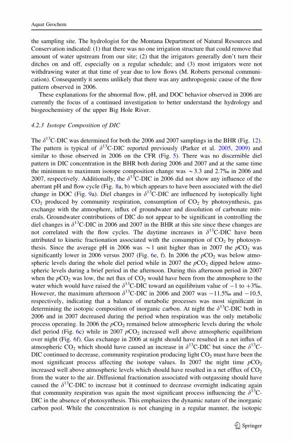
4.2.3 Isotope Composition of DIC
The d13C-DIC was determined for both the 2006 and 2007 samplings in the BHR (Fig. 12).
The pattern is typical of d13C-DIC reported previously (Parker et al. 2005, 2009) and
similar to those observed in 2006 on the CFR (Fig. 5). There was no discernible diel
pattern in DIC concentration in the BHR both during 2006 and 2007 and at the same time
the minimum to maximum isotope composition change was *3.3 and 2.7% in 2006 and
2007, respectively. Additionally, the d13C-DIC in 2006 did not show any influence of the
aberrant pH and flow cycle (Fig. 8a, b) which appears to have been associated with the diel
change in DOC (Fig. 9a). Diel changes in d13C-DIC are influenced by isotopically light
CO2 produced by community respiration, consumption of CO2 by photosynthesis, gas
exchange with the atmosphere, influx of groundwater and dissolution of carbonate min-
erals. Groundwater contributions of DIC do not appear to be significant in controlling the
diel changes in d13C-DIC in 2006 and 2007 in the BHR at this site since these changes are
not correlated with the flow cycles. The daytime increases in d13C-DIC have been
attributed to kinetic fractionation associated with the consumption of CO2 by photosyn-
thesis. Since the average pH in 2006 was *1 unit higher than in 2007 the pCO2 was
significantly lower in 2006 versus 2007 (Fig. 6e, f). In 2006 the pCO2 was below atmo-
spheric levels during the whole diel period while in 2007 the pCO2 dipped below atmo-
spheric levels during a brief period in the afternoon. During this afternoon period in 2007
when the pCO2 was low, the net flux of CO2 would have been from the atmosphere to the
water which would have raised the d13C-DIC toward an equilibrium value of -1 to ?3%.
However, the maximum afternoon d13C-DIC in 2006 and 2007 was -11.5% and -10.5,
respectively, indicating that a balance of metabolic processes was most significant in
determining the isotopic composition of inorganic carbon. At night the d13C-DIC both in
2006 and in 2007 decreased during the period when respiration was the only metabolic
process operating. In 2006 the pCO2 remained below atmospheric levels during the whole
diel period (Fig. 6c) while in 2007 pCO2 increased well above atmospheric equilibrium
over night (Fig. 6f). Gas exchange in 2006 at night should have resulted in a net influx of
atmospheric CO2 which should have caused an increase in d13C-DIC but since the d13C-
DIC continued to decrease, community respiration producing light CO2 must have been the
most significant process affecting the isotope values. In 2007 the night time pCO2
increased well above atmospheric levels which should have resulted in a net efflux of CO2
from the water to the air. Diffusional fractionation associated with outgassing should have
caused the d13C-DIC to increase but it continued to decrease overnight indicating again
that community respiration was again the most significant process influencing the d13C-
DIC in the absence of photosynthesis. This emphasizes the dynamic nature of the inorganic
carbon pool. While the concentration is not changing in a regular manner, the isotopic
Aquat Geochem
123

composition of the pool was being modified by changing metabolic rates in this highly
productive system and this was reflected by the diel pattern of d13C-DIC.
5 Conclusions
Diel concentration cycles in DOC were observed in both the CFR and the BHR in 2006 but
very different temporal patterns were observed in these two rivers. No change in DOC
concentration was observed at the same location in the BHR approximately 1 year later
(2007) suggesting that the presence of diel changes in DOC concentration are dependent on
conditions that can change from year-to-year such as different flow regimes (Fig. 6b, e).
The average flow in the BHR in 2007 was *1.7 times higher than in 2006 and had a
different temporal pattern suggesting that the presence of the observed diel changes in
DOC may be linked to circumstances present during extreme low, base flow conditions.
During these extreme low flow events the volume of water in the river is low in relation to
the mass of attached periphyton which could amplify effects such as instream damming
caused by aquatic plants and algae. These hydrologic and biogeochemical dynamics are
not well understood and are the subjects of further study.
The DOC cycle in the BHR in 2006 reached a maximum concentration at *01:00, which
is approximately the time that the flow reached its maximum (Fig. 6b, 7). The pH during the
2006 sampling showed an unusual bi-phasic pattern with a maximum around 14:00 and then
again at about 02:00. Between these two maximums there was a steep drop in pH with a
minimum at *17:00; coincident with the steep drop in flow. Normally pH will reach a
minimum in the early morning (*07:00 in 2007, Fig. 6d). This pH increase during the night
could not have been caused directly by photosynthesis removing CO2 from the water.
However, since the flow increased at the same time this pattern is consistent with a mass of
water moving into this reach that was chemically modified (higher pH, lower conductivity).
Two hypotheses that have been suggested above to explain these data are: (1) increased flow
from streamside regions and/or benthic sediments at night as evapo-transpiration decreased;
-10
2007
‰) -12
-11
δ13C
-DIC
(
-14
-13
2006
-16
-15
20:00 02:00 08:00 14:00 20:00 02:00 08:00 14:00Day 1 Day 2
Fig. 12 d13C-DIC at the BHR site during the 2006 (blue squares) and 2007 (open circles) during dielsamplings. Error bars represent 3% RSD based on duplicate determinations
Aquat Geochem
123

and (2) the possibility that algae and macrophytes in upstream reaches float up and partially
dam the river during the day due to photosynthesis and then sink at night, releasing the
water. The second hypothesis has been suggested to explain the large diel changes in flow
previously observed in this middle reach of the BHR of up to 2.8 m3 s-1 (100% minimum to
maximum) in a period of as little as 2 h (USGS gage data, not shown). These large flow
cycles observed in the past have had similar timing and trends to those of the 2006 flow
reported in this study.
The first explanation is partially supported by preliminary results of samples collected
from a number of seeps along the BHR above the sampling site in 2007. The water from
these seeps had DOC concentrations *4-times higher on the average than the river
(Fig. 11). At the same time water extracted from shallow benthic sediments had DOC
concentrations similar to that of the river. The pH of the water from the seeps was in
general lower than that of the river (avg., 6.8 vs. 8.1; Table 1). Consequently, this makes it
seem unlikely that the increase in pH in conjunction with the increase in DOC observed in
2006 was due to a large influx of water from bank storage in streamside areas above the
sampling site.
The latter explanation predicts a ‘‘slug’’ of water moving downstream that would be of
higher pH due to photosynthetic removal of CO2 during the day and have a higher con-
centration of DOC due to leakage of soluble organic photosynthates. It is interesting to
note that the d13C-DIC during both 2006 and 2007 had the same pattern and in 2006
appeared to show no influence from the observed flow and pH increase during the night
(Fig. 11). This suggests that the biologic processing of inorganic carbon is acting at a time
scale resulting in a ‘‘normal’’ d13C-DIC pattern.
In the CFR, the DOC showed an inverse temporal pattern to that observed in the BHR in
2006. The DOC in the CFR reached a maximum concentration at *16:00 which is con-
sistent with ‘‘leakage’’ of photosynthates during this active photosynthetic period. The
d13C-DOC became isotopically depleted during the afternoon most likely due to incor-
poration of ‘‘light’’ organics produced by photosynthesis and then became enriched during
the night as microbial oxidation of DOC consumed lighter carbon containing compounds at
a faster rate. It is also possible that the isotopically heavier DOC is in part a different class
of compounds that was more recalcitrant and less readily oxidized than the isotopically
lighter, recently synthesized compounds. Additionally, a comparison of the rates of change
in the concentration of DOC and DIC indicates that the night time increase in DIC can not
be solely attributed to microbial oxidation of DOC.
This study emphasizes the importance of the need for a better understanding of the
dynamic nature of diel changes in the concentration of both dissolved inorganic and
organic species in rivers. It also underscores the fact that different patterns of DOC con-
centration can occur seasonally in the same aquatic system. Additionally, it demonstrates a
need to better quantify the types of organic compounds included in the DOC pool in
relation to both the isotopic composition as well as how readily available these forms are
for heterotrophic oxidation. These results also highlight the fact that significant short term
temporal changes in DOC can occur and monitoring protocols for DOC need to take diel
concentration changes into account. Also, predicting diel concentration patterns based on
prior behavior may not always be reliable as shown by the BHR results for 2006 and 2007.
The night time pH maximum observed in the BHR during 2006 that coincided with the
large concentration increase of DOC suggests that these two occurrences may have been
caused by the same process which is also related to the simultaneous increase in flow.
Unfortunately, these ‘‘anomalous’’ flow occurrences don’t happen every year as seen in
2007 but do need to be further investigated when they do happen. This may lead to
Aquat Geochem
123

significant insight into the function and response of riverine systems to drought/low flow
and changing land use conditions.
Acknowledgments We thank Heiko Langer, David Nimick and Blaine McClesky for their help withanalytical work. Chris Gammons has been an invaluable resource of information on the CFR and BHR andprovided productive critical insight for this work. This work was funded by the Montana Water Centerthrough a grant from the USGS 104(b) Water Resources Research Program as well as the Montana TechUndergraduate Research Program. S. Poulson was funded by NSF, EAR-0738912. This manuscript wasgreatly improved by the comments of two anonymous reviewers.
References
Amon RMW, Benner R (1996) Bacterial utilization of different size classes of dissolved organic matter.Limniol Ocenaogr 41:41–51
Barth JAC, Veizer J (1999) Carbon cycle in St. Lawrence aquatic ecosystems at Cornwall (Ontario),Canada: seasonal and spatial variations. Chem Geol 159:107–128
Bianchi TS, Filley T, Dria K, Hatcher PG (2004) Temporal variability in sources of organic carbon in thelower Mississippi River. Geochim Cosmochim Acta 68:959–967
Bianchi TS, Wysocki LA, Stewart M, Filley TR, McKee BA (2007) Temporal variability in terrestrial-derived sources of particulate organic carbon in the lower Mississippi River and its upper tributaries.Geochim Cosmochim Acta 71:4425–4437
Bond BJ, Jones JA, Moore G, Phillips N, Post D, McDonnell JJ (2002) The zone of vegetation influence onbaseflow revealed by diel patterns of streamflow and vegetation water use in a headwater basin. HydrolProcess 16:1671–1677
Brick CM, Moore JN (1996) Diel variation of trace metals in the upper Clark Fork River, Montana. EnvironSci Technol 30:1953–1960
Clapp CE, Hayes MHB, Senesi N, Griffith SM (eds) (1998) Humic substances and organic matter in soil andwater environments: characterization, transformations, and interactions. International Humic Sub-stances Society, Inc., St. Paul
Clark ID, Fritz P (1997) Environmental isotopes in hydrogeology. Lewis Pub, New YorkDalzell BJ, Filley TR, Harbor JM (2007) The role of hydrology in annoual organic carbon loads and
terrestrial organic matter export from a Midwestern agricultural watershed. Geochim Cosmochim Acta71:1448–1462
Duff BC (2001) Arsenic treatability study utilizing aeration and iron adsorption-coprecipitation at the WarmSprings Ponds. MS thesis, Montana Tech. Butte, MT USA
Falkowski PG, Raven JA (1997) Aquatic photosynthesis. Blackwell Sciences, MaldenGaiero D, Probst JL, Depetris PJ, Gauthier-Lafaye F, Stille P (2005) d13C tracing of dissolved inorganic
carbon sources in Patagonian rivers (Argentina). Hydrol Process 19(17):3321–3344Gammons CH, Ridenour R, Wenz A (2001) Diurnal and longitudinal variations in water quality along the
Big Hole River and tributaries during the drought of August, 2000. Mont Bur Mines Geol 424:39Open-File Report
Gammons CH, Nimick DA, Parker SR, Cleasby TE, McClesky RB (2005) Diel behavior of iron and otherheavy metals in a mountain stream with acidic to neutral pH: Fisher Creek, MT, USA. GeochimCosmochim Acta 69:2505–2516
Gammons CH, Grant TM, Nimick DA, Parker SR, DeGrandpre MD (2007) Diel changes in water chemistryin an arsenic-rich stream and treatment-pond system. Sci Total Env 384:433–451
Gandhi H, Wiegner TN, Ostrom PH, Kaplan LA, Ostrom NE (2004) Isotopic (13C) analysis of dissolvedorganic carbon in stream water using an elemental analyzer coupled to a stable isotope mass spec-trometer. Rapid Commun Mass Spectrom 18:903–906
Harris D, Porter LK, Paul EA (1997) Continuous flow isotope ratio mass spectrometry of carbon dioxidetrapped as strontium carbonate. Commun Soil Sci Plant Anal 28:747–757
Harrison JA, Matson PA, Fendorf SE (2005) Effects of a diel oxygen cycle on nitrogen transformations andgreenhouse gas emissions in a eutrophied subtropical stream. Aquat Sci 67(3):308–315
Hobbie JE (1992) Microbial control of dissolved organic carbon in lakes—research for the future. Hyd-robiologia 229:169–180
Hood E, Williams MW, McKnight DM (2005) Sources of dissolved organic matter (DOM) in a rockymountain stream using chemical fractionation and stable isotopes. Biogeochemistry 74(2):231–255
Aquat Geochem
123

Hrncir DC, McKnight D (1998) Variation in photoreactivity of iron hydroxides taken from an AcidicMountain Stream. Environ Sci Technol 32:2137–2141
Jones CA, Nimick DA, McCleskey B (2004) Relative effect of temperature and pH on diel cycling ofdissolved trace elements in Prickly Pear Creek, Montana. Water Air Soil Pollut 153:95–113
Kaplan LA, Bott TL (1982) Diel fluctuations of DOC generated by algae in a piedmont stream. LimnolOceanogr 27(6):1091–1100
Lewis E, Wallace DWR (1998) Program developed for CO2 system calculations. ORNL/CDIAC-105.Carbon Dioxide Information Analysis Center, Oak Ridge National Laboratory, U.S. Department ofEnergy, Oak Ridge, Tennessee; http://cdiac.ornl.gov/oceans/co2rprt.html
Macalady DL (ed) (1998) Perspectives in environmental chemistry. Oxford University Press, New YorkManny BA, Wetzel RG (1973) Diurnal changes in dissolved organic and inorganic carbon and nitrogen in a
hardwater stream. Freshw Biol 3:31–43McKnight DM, Harnish R, Wershaw RL, Baron JS, Schiff S (1997) Chemical characteristics of particulate,
colloidal and dissolved organic material in Loch Vale Watershed, Rocky Mountain National Park.Biogeochemistry 36:99–124
Moore JN, Luoma SN (1990) Hazardous wastes from large-scale metal extraction. Environ Sci Technol24:1279–1285
Nagorski SA, Moore JN, McKinnon TE, Smith DB (2003) Scale-dependent temporal variations in streamwater geochemistry. Environ Sci Technol 37:859–864
Nimick DA, Gammons CH, Cleasby TE, Madison JP, Skaar D, Brick CM (2003) Diel cycles in dissolvedmetal concentrations in streams—occurrence and possible causes. Water Resour Res 39:1247. doi:10.1029/WR001571
Nimick DA, Cleasby TE, McClesky RB (2005) Seasonality of diel cycles of dissolved trace metal con-centrations in a Rocky Mountain Stream. Env Geol 47:603–614
NOAA (2008) Climate monitoring and diagnostics laboratory, carbon cycle greenhouse gases 2008.http://www.cmdl.noaa.gov/ccgg/iadv
Odum HT (1956) Primary production in flowing waters. Limnol Oceanogr 1:102–117Olivie-Lanquet G, Gruau G, Dia A, Riou C, Jaffrezic A, Henin O (2001) Release of trace elements in
wetlands: role of seasonal variability. Water Res 35(4):943–952Parker SR, Poulson SR, Gammons CH, DeGrandpre MD (2005) Biogeochemical controls on diel cycling of
stable isotopes of dissolved oxygen and dissolved inorganic carbon in the Big Hole River, Montana.Environ Sci Technol 39:7134–7140. doi:10.1021/es0505595
Parker SR, Gammons CH, Poulson SR, DeGrandpre MD (2007a) Diel changes in pH, dissolved oxygen,nutrients, trace elements, and the isotopic composition of dissolved inorganic carbon in the upper ClarkFork River, Montana, USA. Appl Geochem 22:1329–1343. doi:10.1016/j.apgeochem.2007.02.007
Parker SR, Gammons CH, Jones CA, Nimick DA (2007b) Role of hydrous iron oxide formation in atten-uation and diel cycling of dissolved trace metals in a stream affected by acid rock drainage. Water AirSoil Pollut 181:247–2663. doi:10.1007/s11270-006-9297-5
Parker SR, Gammons CH, Poulson SR, Weyer CL, Smith MG, Babcock JN, Oba Y (2009) Diel behavior ofstable isotopes (18-O & 13-C) of dissolved oxygen and dissolved inorganic carbon in Montana, USArivers, and in a mesocosm experiment. Chemical Geology. doi:10.1016/j.chemgeo.2009.06.016
Parkhurst DL, Appelo CAJ (1999) User’s guide to PHREEQC (Version 2)—a computer program forspeciation, batch-reaction, one-dimensional transport, and inverse geochemical calculations: U.S.Geological Survey Water-Resources Investigations Report 99-4259: 310, http://wwwbrr.cr.usgs.gov/projects/GWC_coupled/phreeqc/
Pogue TR, Anderson CW (1994) Processes controlling dissolved oxygen and pH in the Upper WillametteRiver Basin. US Geol Surv. Water-Resources Investigations Report 95-4205
Poole GC, O’Daniel SJ, Jones KL, Woessner WW, Bernhardt ES, Helton AM, Stanford JA, Boer BR,Beechie TJ (2008) Hydrological spiraling: the role of multiple interactive flow paths in stream eco-systems. River Res Applic 24(7):1018–1031. doi 10.1002/rra.1099
Ridenour R (2002) A seasonal and spatial chemical study of the Big Hole River, Southwest Montana. M.S.Thesis, Montana Tech of The University of Montana, Butte, MT
Saar RA, Weber JH (1982) Fulvic acid: modifier of metal-ion chemistry. Environ Sci Technol 16:510A–517A
Spencer RGM, Pellerin BA, Bergamaschi BA, Downing BD, Kraus TEC, Smart DR, Dahlgren RA, HernesPJ (2007) Diurnal variability in riverine dissolved organic matter compostion determined by in situoptical measurements in the San Joaquin River (California, USA). Hydrol Process 21:3181–3189. doi:10.1002/hyp.6887
Thurman EM (1985) Organic geochemistry of natural waters. Kluwer Acad. Pub, Boston
Aquat Geochem
123

Usdowski E, Hoefs J, Menschel G (1979) Relationship between 13C and 18O fractionation and changes inmajor element composition in a recent calcite-depositing spring—a model of chemical variations withinorganic CaCO3 precipitation. Earth Planet Sci Lett 42:267–276
Voelker BM, Morel BM, Sulzberger B (1997) Iron redox cycling in surface waters: effects of humicsubstances and light. Environ Sci Technol 31:1004–1111
Volk CJ, Volk CB, Kaplan LA (1997) Chemical composition of biodegradable dissolved organic matter instreamwater. Limnol Oceanogr 42(1):39–44
Vymazal J (1994) Algae and element cycling in wetlands. Lewis Publishers, CRC Press, Inc., Boca Raton, p222
Watson V (1989) Maximum levels of attached algae in the Clark Fork River. Proc Mont Acad Sci 49:27–35Wenz AC (2003) Diurnal variations in the water quality of the Big Hole River. M.S. Thesis, Montana Tech
of The University of Montana, Butte, MTWetzel RG, Likens GE (1991) Limnological analysis, 2nd edn. Springer-Verlag, NYZeigler SE, Brisco SL (2004) Relationships between the isotopic composition of dissolved organic carbon
and its bioavailability in contrasting Ozark streams. Hydrobiologia 513:153–169Zeigler SE, Fogel ML (2003) Seasonal and diel relationships between the isotopic compositions of dissolved
and particulate organic matter in freshwater ecosystems. Biogeochemistry 64:25–52
Aquat Geochem
123
Temporal and spatial changes in the concentration andisotopic composition of nutrients in the upper Silver BowCreek drainage, Montana: Year 2
Basic Information
Title: Temporal and spatial changes in the concentration and isotopic composition of nutrientsin the upper Silver Bow Creek drainage, Montana: Year 2
Project Number: 2007MT145BStart Date: 3/1/2007End Date: 12/31/2008
Funding Source: 104BCongressional
District: at large
ResearchCategory: Water Quality
Focus Category: Nitrate Contamination, Hydrogeochemistry, Surface WaterDescriptors:
PrincipalInvestigators: Chris Gammons
Publication
Plumb, Beverly 2009 Geochemistry of Nutrients in Silver Bow Creek, Butte, Montana "MSDissertation" Department of Geoscience, Montana Tech of the University of Montana, Butte, MT 85pgs
1.
Temporal and spatial changes in the concentration and isotopic composition of nutrients in the upper Silver Bow Creek drainage, Montana: Year 2
Temporal and spatial changes in the concentration and isotopic composition of nutrients in the upper Silver Bow Creek drainage, Montana: Year 21
Temporal and spatial changes in the concentration and isotopic composition
of nutrients in the upper Silver Bow Creek drainage, Montana: Year 2
Primary Investigator: Dr. Chris Gammons
Department of Geological Engineering
Montana Tech of the University of Montana
2009

1
Abstract
From the late 1800‟s to the 1970‟s, mine waste from mining activities in the
Butte, Montana area was discharged into Silver Bow Creek. This created a toxic
environment and destroyed most of the aquatic life in the stream. Beginning in 1999 and
continuing to the present day, extensive reclamation activities along Silver Bow Creek
and the historic mining district have improved environmental conditions in the Butte
area, and metal concentrations in upper Silver Bow Creek now meet aquatic life
standards. However, previous work has shown the existence of very high nutrient
concentrations in Silver Bow Creek. Now that the metal toxicity has been eliminated,
symptoms of severe eutrophication are evident, such as uncontrolled growth of aquatic
plants and algae.
This research examined the geochemistry of nutrients (nitrate, nitrite, ammonia,
phosphate) in upper Silver Bow Creek, with special attention to spatial and seasonal
changes in nutrient concentrations and loads. Synoptic samples for nutrient analysis were
collected at 10 to 15 monitoring locations every 4-6 weeks, beginning in May of 2006
and ending in August of 2007. Samples were collected on a regular basis at 4 sites on
Blacktail Creek, at the mouth of Basin Creek, at 3 sites on upper Silver Bow Creek
upstream of Rocker, and at the points-of-discharge from the Montana Pole, Lower Area
One, and Butte Silver Bow wastewater treatment plant (WWTP) facilities. The results
show that nutrient concentrations and loads in Silver Bow Creek as it leaves the Butte
Summit Valley are very high, even when compared to national reference conditions for
„developed basins‟. The largest nutrient source is the WWTP, which contributes over
80% of the total N load, mainly in the form of ammonia (NH4+ + NH3). This ammonia is
then gradually oxidized to nitrate, resulting in a substantial increase in the concentration
and load of nitrate as Silver Bow Creek makes its way from Butte to Rocker. The
oxidation process consumes dissolved oxygen (DO), and creates very low DO
concentrations, in some cases to values less than 1 mg/L. Because the oxidation of
ammonia to nitrate is faster in warm vs. cold water, the nighttime depletion of DO is most
extreme during summer baseflow conditions. Diurnal changes in the rate of ammonia
oxidation also result in 24-h changes in the concentrations of ammonia and nitrate in
Silver Bow Creek.
Two sets of samples were also collected in this study for analysis of δ15
N-nitrate,
δ18
O-nitrate and δ15
N-ammonia. The results show that both forms of N in Silver Bow
Creek (ammonia, nitrate) are consistent with having been derived primarily from human
and animal waste. There are few if any consistent differences between the isotopic
compositions of the various point sources and non-point sources of N in the watershed.
Attempts to use isotopes to fingerprint sources of nutrients are further complicated by the
fact that in-stream fractionation of N-isotopes occurs during bacterial oxidation of
ammonia to nitrate.

2
1.0 INTRODUCTION
1.1 Research Objectives
Starting in the late 1800‟s mine waste containing high metal concentrations from
the mining, milling and smelting in and around Butte, MT was discharged into Silver
Bow Creek. These high metal concentrations created a toxic environment in Silver Bow
Creek and virtually annihilated aquatic life (Moore and Luoma, 1990). Beginning in
1999, a massive cleanup effort began to remove toxic tailings from the Silver Bow Creek
floodplain, to reconstruct a new stream channel, and to reestablish floodplain and
streamside vegetation. Restoration of the upper 10 km of Silver Bow Creek is now
complete, and already there are signs that trout are returning to the stream (Frandsen,
2006; Forsell, 2006). However, whereas huge progress has been made to remove metals
contamination from Silver Bow Creek, another serious issue has been neglected nutrient
overload.
Although nutrients such as nitrate (NO3-) and phosphate (PO4
3-) are essential for
all forms of life, too many nutrients in a stream environment can have undesirable effects
(e.g., Redfield, 1958; Mueller and Helsel, 1996). These include rapid growth of algae
and weeds, increase in turbidity, blockage of sunlight, and large seasonal and diurnal (24-
h) swings in pH and dissolved oxygen (DO) concentration. Collectively, these symptoms
are often referred to as eutrophication. Nutrient levels in the Clark Fork River watershed
are elevated, due to both point- and non-point source pollution (Samuels and Hallock,
1994; Watson and Gestring, 1996; Dodds et al., 1997; TSWQC, 2005, 2007). The former

3
include municipal sewage effluents, industrial discharges, and livestock feedlots. The
latter include septic tanks, fertilizers, and domestic animal waste.
The main objective of this research was to collect samples of upper Silver Bow
Creek and its main tributaries over a 16 month period to determine spatial and seasonal
trends in nutrient concentrations and loads (load = concentration x stream discharge).
The city of Butte is located at the headwaters of the Clark Fork watershed, and therefore
any nutrients leaving the study area have an impact on downstream waters, including
Silver Bow Creek and the upper Clark Fork River. Another objective was to collect
preliminary information on the stable isotopic composition of nitrate and dissolved
ammonium (NH4+) in Silver Bow Creek as well as the known point-sources of high N
contamination. These data were then used to test if stable isotopes have potential to be
used as tracers of the origins or chemical transformations of N throughout the upper
Clark Fork watershed, as has been shown to be the case in previous studies elsewhere
(e.g., Coplen, 1993; Wassenaar, 1995; Bohlke and Denver, 1996; Kendall, 1998; Kellman
and Hillaire-Marcel, 2003; Deutsch et al., 2005).
1.2 Site Description
Silver Bow Creek begins at the confluence of Blacktail Creek and the Metro
Strom Drain (MSD) in Butte, MT (Fig. 1). As of this writing, the population of Butte,
MT is around 31,000. However, in the “heyday” of mining in the mid-1900s Butte is
reported to have had a population of > 80,000 people. The average low temperature in
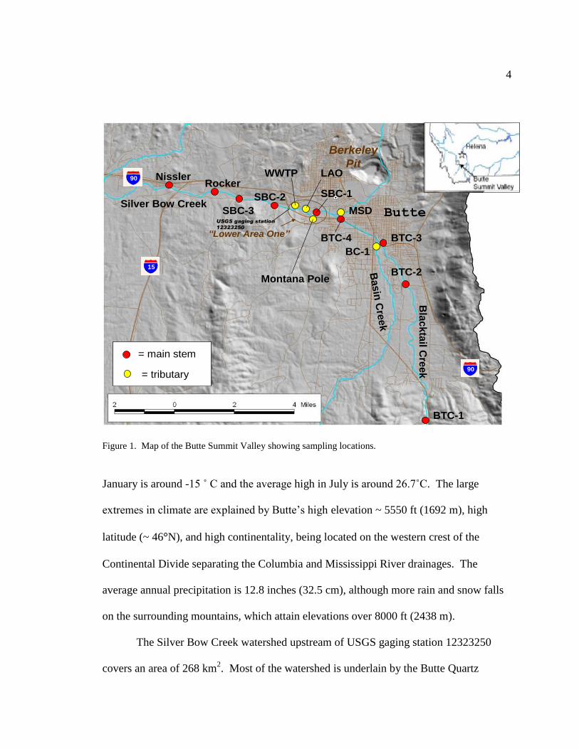
4
= main stem
= tributary
= main stem
= tributary
Bla
ckta
ilC
reek
Basin
Cre
ek
Silver Bow CreekButte
Montana Pole
LAOWWTP
1515
9090
1515
9090
Berkeley
Pit
BTC-1
BTC-2
BTC-3
BC-1
MSD
BTC-4
SBC-1
““Lower Area OneLower Area One””
NisslerRocker
SBC-3
SBC-2
Nissler Rocker
USGS gaging station
12323250
= main stem
= tributary
= main stem
= tributary
Bla
ckta
ilC
reek
Basin
Cre
ek
Silver Bow CreekButte
Montana Pole
LAOWWTP
1515
9090
1515
9090
Berkeley
Pit
BTC-1
BTC-2
BTC-3
BC-1
MSD
BTC-4
SBC-1
““Lower Area OneLower Area One””
NisslerRocker
SBC-3
SBC-2
Nissler Rocker
USGS gaging station
12323250
= main stem
= tributary
= main stem
= tributary
Bla
ckta
ilC
reek
Basin
Cre
ek
Silver Bow CreekButte
Montana Pole
LAOWWTP
1515
9090
1515
9090
Berkeley
Pit
BTC-1
BTC-2
BTC-3
BC-1
MSD
BTC-4
SBC-1
““Lower Area OneLower Area One””
NisslerRocker
SBC-3
SBC-2
Nissler Rocker
USGS gaging station
12323250
Figure 1. Map of the Butte Summit Valley showing sampling locations.
January is around -15 ˚ C and the average high in July is around 26.7˚C. The large
extremes in climate are explained by Butte‟s high elevation ~ 5550 ft (1692 m), high
latitude (~ 46 N), and high continentality, being located on the western crest of the
Continental Divide separating the Columbia and Mississippi River drainages. The
average annual precipitation is 12.8 inches (32.5 cm), although more rain and snow falls
on the surrounding mountains, which attain elevations over 8000 ft (2438 m).
The Silver Bow Creek watershed upstream of USGS gaging station 12323250
covers an area of 268 km2. Most of the watershed is underlain by the Butte Quartz
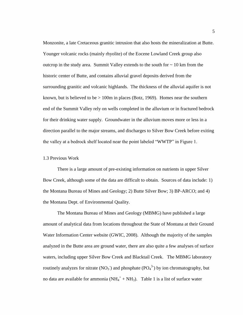
5
Monzonite, a late Cretaceous granitic intrusion that also hosts the mineralization at Butte.
Younger volcanic rocks (mainly rhyolite) of the Eocene Lowland Creek group also
outcrop in the study area. Summit Valley extends to the south for ~ 10 km from the
historic center of Butte, and contains alluvial gravel deposits derived from the
surrounding granitic and volcanic highlands. The thickness of the alluvial aquifer is not
known, but is believed to be > 100m in places (Botz, 1969). Homes near the southern
end of the Summit Valley rely on wells completed in the alluvium or in fractured bedrock
for their drinking water supply. Groundwater in the alluvium moves more or less in a
direction parallel to the major streams, and discharges to Silver Bow Creek before exiting
the valley at a bedrock shelf located near the point labeled “WWTP” in Figure 1.
1.3 Previous Work
There is a large amount of pre-existing information on nutrients in upper Silver
Bow Creek, although some of the data are difficult to obtain. Sources of data include: 1)
the Montana Bureau of Mines and Geology; 2) Butte Silver Bow; 3) BP-ARCO; and 4)
the Montana Dept. of Environmental Quality.
The Montana Bureau of Mines and Geology (MBMG) have published a large
amount of analytical data from locations throughout the State of Montana at their Ground
Water Information Center website (GWIC, 2008). Although the majority of the samples
analyzed in the Butte area are ground water, there are also quite a few analyses of surface
waters, including upper Silver Bow Creek and Blacktail Creek. The MBMG laboratory
routinely analyzes for nitrate (NO3-) and phosphate (PO4
3-) by ion chromatography, but
no data are available for ammonia (NH4+ + NH3). Table 1 is a list of surface water

6
sampling sites for which historical chemical data are available in GWIC. Additional data
exist on GWIC for sampling locations in the Lower Area One region that no longer exist,
due to re-construction activities. As an example, Figure 2 shows GWIC data for Silver
Bow Creek collected at USGS gaging station 12323250, which is located immediately
downstream of the point of discharge for the Butte waste water treatment plant (WWTP).
The data are inconsistent, both in terms of the concentrations measured and also with
respect to the timing of when the samples were collected. Nonetheless, the results show
many sampling dates with highly elevated nutrient concentrations (e.g., greater than 1
mg/L N or P), underscoring the nature of the nutrient problem in the watershed. Data
collected by MBMG are fewer for most of the other Silver Bow Creek sampling stations
listed in Table 1, and are not shown here.
. Table 1. Surface water sampling station in GWIC database.
GWIC ID# Description Site name, this
research
127593 Blacktail Creek at USGS gage 12323240 BTC-4
127536 Silver Bow Creek below Blacktail Creek
217884 Silver Bow Creek above MT Pole, SW-06a SBC-1
164317 Silver Bow Creek below MT Pole, SW-05
161467 Montana Pole effluent MT Pole
4851 BSB Sewage Treatment Plant effluent WWTP
4930 Silver Bow Creek at USGS gage 12323250
196457 Silver Bow Creek at SS-08, upstream of Rocker SBC-3
217882 Silver Bow Creek at SS-14
149881 Silver Bow Creek at Miles Crossing

7
0.1
1
10
Jan-
82
Jan-
84
Jan-
86
Jan-
88
Jan-
90
Jan-
92
Jan-
94
Jan-
96
Jan-
98
Jan-
00
Jan-
02
Jan-
04
co
ncen
trati
on
, m
g/L
as N
or
P
NO3 PO4
Figure 2. Concentrations of nitrate and phosphate in Silver Bow Creek at USGS gaging station 12323250
between 1982 and 2003. Data from GWIC (2008).
In 2004, the MBMG published a report (Carstarphen et al., 2004) that
documented the occurrence of elevated nitrate levels in many shallow groundwater wells
in the Butte Summit Valley. This report also included results from two synoptic
sampling events along Blacktail Creek and upper Silver Bow Creek, down to the USGS
gaging station 12323250. The study concluded that there were significant loadings of
nitrate to Blacktail Creek as it makes its way through the Butte Summit Valley, and that
the most likely cause of this nutrient contamination was groundwater influx. Carstarphen
et al. (2004) also published some stable isotopic results for 18
O and 15
N of nitrate in
Butte groundwater wells and concluded that the main source of nitrate was not synthetic
fertilizer, but more likely human and/or animal waste. The more recent report of LaFave

8
(2008) expanded on the earlier work of Carstarphan et al. (2004), and drew similar
conclusions.
During 2003-2004, a study was conducted on concentrations of nutrients in upper
Silver Bow Creek by Water & Environmental Technologies, Inc. (WET, 2004). This
one-year study gathered data from 8 locations in the watershed, including several stations
sampled in the present research. The overall conclusions of the study were that upper
Silver Bow Creek is severely impacted by high concentrations of nutrients, including
nitrate, ammonia, and phosphate. Numerous point and non-point sources of nutrient
contamination were inferred to be present, including the WWTP effluent and other
discharging waters in the Lower Area One area, as well as suspected groundwater gains
in the stream reach extending from Lower Area One downstream to Rocker. This study
was one of the first investigations that documented high concentrations of ammonia in
Silver Bow Creek.
Butte Silver Bow (BSB) monitors the effluent water chemistry from the WWTP
on a monthly basis. Although this information is not freely available, data collected
between 1996 and 2006 were kindly provided by BSB for this research, and are
summarized in Figure 3. This graph shows a gradual increase in the concentrations of
total N and total P in the WWTP effluent during the past 10 years. It also shows that very
little of the nitrogen exiting the plant is present in oxidized form (e.g., as nitrite, NO2-, or
nitrate, NO3-). The majority is ammonia (NH4
+ + NH3), with some additional N in
dissolved organic form (data not shown). The scatter in the data underscores the high
amount of short-term variability in the water quality discharged from the WWTP.
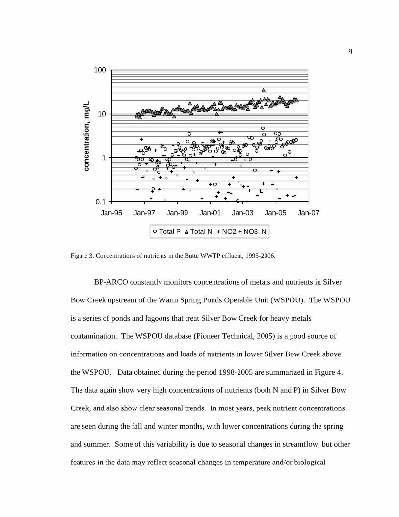
9
0.1
1
10
100
Jan-95 Jan-97 Jan-99 Jan-01 Jan-03 Jan-05 Jan-07
co
ncen
trati
on
, m
g/L
Total P Total N NO2 + NO3, N
Figure 3. Concentrations of nutrients in the Butte WWTP effluent, 1995-2006.
BP-ARCO constantly monitors concentrations of metals and nutrients in Silver
Bow Creek upstream of the Warm Spring Ponds Operable Unit (WSPOU). The WSPOU
is a series of ponds and lagoons that treat Silver Bow Creek for heavy metals
contamination. The WSPOU database (Pioneer Technical, 2005) is a good source of
information on concentrations and loads of nutrients in lower Silver Bow Creek above
the WSPOU. Data obtained during the period 1998-2005 are summarized in Figure 4.
The data again show very high concentrations of nutrients (both N and P) in Silver Bow
Creek, and also show clear seasonal trends. In most years, peak nutrient concentrations
are seen during the fall and winter months, with lower concentrations during the spring
and summer. Some of this variability is due to seasonal changes in streamflow, but other
features in the data may reflect seasonal changes in temperature and/or biological

10
productivity of the stream. For example, it is interesting to note that the
ammonia/(nitrate+nitrite) ratio of water entering the WSPOU is much higher in the
winter than in the summer. This topic will be discussed in a later section of this
research.
Finally, the Montana Dept. of Environmental Quality (MDEQ) has a large amount
of monitoring data on the water quality of upper Silver Bow Creek available upon
request, most of which is summarized in the form of annual reports (e.g., MDEQ, 2006).
0.01
0.1
1
10
Jan-
97
Jan-
98
Jan-
99
Jan-
00
Jan-
01
Jan-
02
Jan-
03
Jan-
04
Jan-
05
Co
nc
en
tra
tio
n, m
g/L
as
N o
r P
ammonia nitrate + nitrite phosphate
Figure 4. Nutrient concentrations in Silver Bow Creek above WSPOU, 1997-2005. Data from Pioneer
Technical (2005).

11
3.0 METHODS
3.1 Field methods
3.1.1 Synoptic sampling
Twelve synoptic sampling events were conducted on Silver Bow Creek for this
research and they occurred in May, June, October, November and December of 2006, and
January, March, April, May, June, July, and August of 2007. Field measurements and
water samples were taken at a number of sites along Silver Bow Creek and its major
tributaries (Figure 1, Table 2
Table 2. Sample sites used in this study.
Site name Location km below
BTC-1
BTC-1 Blacktail Creek at Thompson Park 0
BTC-2 Blacktail Creek at intersection with 4 Mile Road 8.0
BTC-3 Blacktail Creek at Father Sheehan Park 10.4
BC-1 Mouth of Basin Creek, near BTC-3 10.4
BTC-4 Blacktail Creek at Butte Visitors‟ Center, just upstream of
USGS gage 12323240 13.5
MSD Mouth of Butte Metro Storm Drain 13.7
SBC-1 Silver Bow Creek upstream of MT Pole 14.8
MT Pole Point discharge from Montana Pole 14.8
LAO Point discharge from Lower Area One 15.2
WWTP Point discharge from Butte wastewater treatment plant 15.8
SBC-2 Silver Bow Creek at first frontage road bridge below I-90
overpass 16.9
SBC-3 Silver Bow Creek at second frontage road bridge,
upstream of Rocker, MT 18.8
Nissler Silver Bow Creek at old bridge near Nissler, just west of
Interstate 15 overpass 22.5
Fairmont Silver Bow Creek at bridge to Fairmont Hot Springs 39.8
Opportunity Silver Bow Creek at bridge near USGS gage 12323600 45.9

12
The sites include four locations along Blacktail Creek (BTC), the mouth of Basin
Creek (BC), the mouth of the Butte Metro Storm Drain (MSD), the effluent from the
Montana Pole plant (MT Pole), the discharge from the Lower Area One treatment facility
(LAO), the effluent from the Butte Wastewater Treatment Plant (WWTP), and several
locations along Silver Bow Creek (SBC), stretching from Butte to Opportunity. Because
the focus of this research was nutrient loading in the Butte Summit Valley, stations along
Silver Bow Creek downstream of Rocker, MT were sampled infrequently.
Although many agencies collect water quality samples for Silver Bow Creek at
USGS gaging station 12323250, the stream at this location is directly below the
confluence of the WWTP effluent and upper Silver Bow Creek, and is poorly mixed.
The zone of incomplete mixing extends for several hundred meters below the gaging
station. For this reason, SBC-2 was used in this research to monitor nutrient loads in
Silver Bow Creek at the point where it exits the Butte Summit Valley.
Figure 5 shows the hydrograph for Silver Bow Creek at USGS gaging station
12323250 during the 2-year study. Dates of sampling related to this research are shown
by the green squares. It is worth noting that none of the sampling events in this study
captured thunderstorms or major spring runoff events. This was intentional, as it was
reasoned that downstream synoptic trends in nutrient concentrations and loads would be
easier to see during steady, baseflow conditions. Measuring synoptic trends in nutrient
concentrations and loads during storm events was not an original objective of the
research, and would require more manpower and time.

13
0
20
40
60
80
100
120
1/1
/06
3/3
/06
5/3
/06
7/3
/06
9/2
/06
11/2
/06
1/2
/07
3/4
/07
5/4
/07
7/4
/07
9/3
/07
11/3
/07
Flo
w,
cfs
sampling dates, this thesis
Figure 5. Hydrograph for Silver Bow Creek during the study period, showing dates of major sampling
events in this research. Data were obtained from the USGS website for Station 12323250, Silver Bow
Creek below Blacktail Creek.
At each site a width- and depth-integrated water sample was collected in a plastic
1-liter Nalgene bottle by holding the bottle at arms length upstream of the sampler and
then progressing across the creek and up and down the water column. These samples
were then filtered on site to 0.2 µm using a disposable PES syringe filter and transferred
to high density polyethylene bottles for further sample analysis in the lab. These bottles
were stored in a cooler on ice or in a refrigerator until analysis. A Hydrolab MS-5
datasonde was used to measure pH, dissolved oxygen (DO), water temperature, and
specific conductivity (SC). The Hydrolab was calibrated in the laboratory to the
manufacturer‟s instructions on the morning before sampling. Field parameters were
recorded along with the date and time in a field book. Other field measurements, such as
turbidity and alkalinity, were sometimes measured, following the methods outlined
below.

14
Streamflow was measured directly at BTC-1, BTC-2, and BTC-3 using a Marsh-
McBirney current meter, a measuring tape, and a top-setting wading rod. At least 10
velocity measurements were taken across each stream section at a depth of 4/10ths from
the bottom of the streambed. Flows at MT Pole and WWTP were taken within 1 hour of
a field visit from gages within the treatment plants at each site. Steamflows at BTC-4,
SBC-2, and Opportunity were taken from USGS gaging stations 12323240, 12323250,
and 12323600. Streamflows at Basin Creek and LAO were not measured directly, but
instead were approximated using a specific conductivity (SC) mass balance, according to
the following equation:
SC1*Q1 + SC2*Q2 = SC3*Q3
where Q1, Q2 and Q3 are the streamflows of the main stem upstream, the tributary
stream, and the main stem downstream, respectively. By measuring the SC at each
location, and by measuring either Q1 or Q3, it was then possible to estimate Q2, the flow
of the tributary.
3.1.2 Diurnal sampling
On July 11-12, 2006, 10 samples were collected over a 24-h period at three
locations to test for diurnal changes in nutrient concentration. The sites included the
WWTP outfall, SBC-1B (Silver Bow Creek immediately upstream of the WWTP
outfall), and SBC-3 (Silver Bow Creek upstream of Rocker). Samples were collected
manually, filtered in the field, and analyzed for nutrient concentrations as described

15
above. Field measurements of water temperature (T), pH, SC, and DO were collected
during each visit with hand-held meters.
The July diurnal investigation showed extremely low concentrations of dissolved
oxygen at SBC-3 during the night. To further investigate this phenomenon, and to map
out the extent of the night-time oxygen sag, a DO traverse of Silver Bow Creek was made
in the pre-dawn hours of August 6, 2006. Two Montana Tech undergraduate students
started sampling at 4:00 AM and quickly moved downstream from SBC-1B to Nissler,
recording T-pH-SC-DO with the MS-5 datasonde. The last measurements were taken at
5:45 AM, just as the sky was starting to lighten. Also, 24-h profiles in T-pH-SC-DO
were made using a Hydrolab Datasonde 3, a Hydrolab Minisonde 5, and an In-Situ Troll
9000 datasonde at 7 locations between August 14 and 17, 2006. All meters were
calibrated on the morning of 8/14/06. The Datasonde 3 was put into the WWTP outfall,
the Minisonde 5 was put into Silver Bow Creek at SBC-2, and the Troll was put into
Silver Bow Creek immediately above the WWTP outfall (station SBC-1B). The next
morning, the Datasonde 3 was moved to Silver Bow Creek at Rocker (behind the Town
Pump station) and the Troll was moved to station SBC-3. Then, on the morning of
August 16, all three units were moved to Silver Bow Creek at Nissler bridge, and side-
by-side 24-h data sets were collected.
3.1.3 Collection of water samples for stable isotope analysis
Water samples for stable isotopic analysis of δ15
N-nitrate, δ18
O-nitrate and δ15
N-
ammonia were collected on October 10, 2006, and June 26-28, 2007. At each site, 2 x 1

16
gallon HDPE containers were filled with filtered water, using a peristaltic pump and 142
mm diameter, 0.1 µm cellulose-ester filter membranes. The containers were first rinsed
with 50 mL of filtered site water. One of the sample bottles was used for isotopic
analysis of nitrate, while the other was used for ammonia. Duplicate filtered samples
were collected in smaller plastic bottles for conventional nutrient analysis (see below),
and field parameters were obtained using the MS-5 datasonde. Both bottles were filled to
near volume and were frozen (the plastic bottles expanded upon freezing but did not
break or leak). The bottles were shipped in a cooler to the stable isotope laboratory at the
University of Waterloo, Ontario. Because of a lab error, no ammonia isotope results
were obtained for the 2007 sampling.
3.2 Analytical Methods
3.2.1 Alkalinity
Alkalinity was measured by taking a raw, unfiltered sample and titrating it with a
HACH digital titrator and 0.16 or 1.6 N sulfuric acid cartridges. A 100 mL volume of
water was measured in a volumetric flask to obtain accurate volumes. Then the 100 mL
sample was poured into an Erlenmeyer flask with a stirring rod. The Erlenmeyer flask
was placed on a battery-operated stir plate. A bromcresol green-methyl red indicator
packet was added to the flask and the stirrer was turned on to make sure adequate mixing
took place. The solution started out blue-green in color (alkaline) and turned pinkish-red
at the pH endpoint of 4.5. The alkalinity (units of mg/L CaCO3, eq) was then measured
directly from the readout on the titrator.
17
3.2.2 Turbidity
Turbidity measurements were taken in the field with a HACH 2100P portable
turbidimeter. The 1-L composite sample bottle was used, and was shaken to re-suspend
any solids before loading the cuvette for the instrument. Two measurements were taken
on each sample and the average of the measurements was used. The turbidimeter was
periodically calibrated with standards ranging between 0 and 100 NTU (Nephelometric
Turbidity Units).
3.2.3 Ammonia
Filtered and refrigerated samples were analyzed for total dissolved ammonia
(NH4+ + NH3) within 12-h of collection using a HACH portable spectrophotometer. The
Nessler Method (HACH method 8038) was used, which is accurate for a range of 0.02 to
2.50 mg/L NH3 as N. The Nessler Method uses the Nessler Reagent, which is a solution
of potassium tetraiodomercurate(II) in potassium hydroxide. The Nessler Reagent reacts
with ammonia and gives a yellow color. Waste from this procedure contains mercury
and was therefore treated as hazardous waste. The colorimeter was zeroed with a
solution of deionized (DI) water to which the HACH reagents were added. Calibration
was checked during each analytical session by running at least one standard solution
containing 0.1 to 1.0 mg/L NH3 as N. Some of the samples collected in this study had
NH3 concentrations above the linear range of the colorimeter, and therefore were diluted
prior to analysis.
18
3.2.4 Nitrite
Filtered and refrigerated samples were analyzed for dissolved nitrite (NO2-) within
12-h of collection using a HACH portable spectrophotometer. The Diazotization Method
(HACH Method 8507) was followed, which uses sulfanilic acid and chromotropic acid
to react with nitrite to produce a pink color. Method 8507 is good for a range of 0.002 to
0.300 mg/L NO2- as N. For samples with high nitrite concentrations, an independent
measure of NO2- was obtained by ion chromatography (IC) (see below). In most cases,
the agreement between the colorimetric and IC results for nitrite was excellent (see
Appendix 3), despite the fact that the sample holding times for IC analysis were often > 1
week. Because of its lower detection limits, all results reported in this research were
obtained by colorimetry unless specified otherwise.
3.2.5 Phosphate
Filtered and refrigerated samples were analyzed for soluble reactive phosphate
(PO43-
) within 12-h of collection using a HACH portable spectrophotometer. The
PhosVer 3 method (HACH Method 8048) was used, in which molybdate is added to the
sample water after pH adjustment, and then ascorbic acid reduces this complex and gives
the solution a blue color. This method is accurate for concentrations of phosphate in the
range of 0.01 to 1.6 mg/L PO43-
as P. The instrument was calibrated during each session
using freshly prepared PO43-
standards. For samples with high phosphate concentrations,
an independent measure of PO43-
was obtained by ion chromatography (IC) (see below).

19
In most cases, the agreement between the colorimetric and IC results for phosphate was
good (see Appendix 3). Because of its lower detection limits, all results reported in this
research were obtained by colorimetry unless specified otherwise.
3.2.6 Nitrate
Early in this project concentrations of dissolved nitrate were determined by
colorimetry, following the Cd-reduction method (HACH Method 8171). However,
laboratory analysis of split samples by IC showed that the colorimetric method was
inaccurate, and therefore was discontinued after June, 2006. After this time, all nitrate
analyses were performed by IC (see below).
3.2.7 Anions/Ion Chromatography
Beginning in July of 2006, all samples collected in this study were analyzed for a
suite of anions by ion chromatography (IC) at the Murdock Environmental Laboratory,
Missoula, MT. Filtered samples for IC analysis were collected in 60 cc HDPE bottles
and stored on ice or in the refrigerator prior to shipment to the Murdock lab. Samples
shipped to Missoula were transported in a small cooler with ice packs, and the samples
were analyzed within 2 weeks of collection. No preservative was added to the bottles.
The Murdock lab followed standard EPA procedures, and provided quantification of
dissolved nitrate, nitrite, phosphate, chloride, sulfate, and fluoride. As pointed out
above, most of the data reported in this research for nitrite and phosphate were obtained
colorimetrically. Nonetheless, the IC results provided a convenient check on the
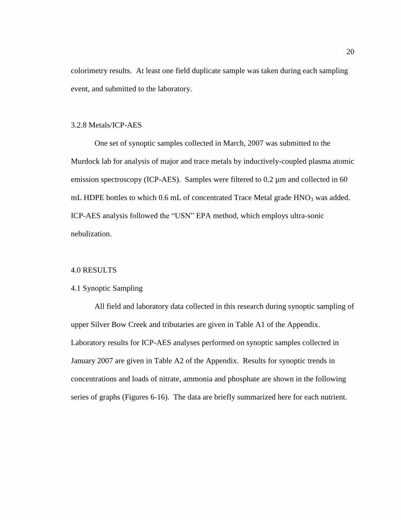
20
colorimetry results. At least one field duplicate sample was taken during each sampling
event, and submitted to the laboratory.
3.2.8 Metals/ICP-AES
One set of synoptic samples collected in March, 2007 was submitted to the
Murdock lab for analysis of major and trace metals by inductively-coupled plasma atomic
emission spectroscopy (ICP-AES). Samples were filtered to 0.2 µm and collected in 60
mL HDPE bottles to which 0.6 mL of concentrated Trace Metal grade HNO3 was added.
ICP-AES analysis followed the “USN” EPA method, which employs ultra-sonic
nebulization.
4.0 RESULTS
4.1 Synoptic Sampling
All field and laboratory data collected in this research during synoptic sampling of
upper Silver Bow Creek and tributaries are given in Table A1 of the Appendix.
Laboratory results for ICP-AES analyses performed on synoptic samples collected in
January 2007 are given in Table A2 of the Appendix. Results for synoptic trends in
concentrations and loads of nitrate, ammonia and phosphate are shown in the following
series of graphs (Figures 6-16). The data are briefly summarized here for each nutrient.

21
4.1.1 Ammonia
Ammonia concentrations and loads were typically low before the addition of the
WWTP at km 15.8. An exception was March 2007, when significant concentrations of
ammonia were detected in lower Blacktail Creek. The source of this ammonia loading
could have been melting of valley snow and washing of animal waste stored over the
winter period into the streams. However, on all sampling dates, by far the biggest
increase in ammonia load occurred from the WWTP. The WWTP effluent averaged
about 12 mg/L ammonia as N during the study period, which is consistent with historical
data supplied by BSB (Fig. 3). Since the flow of the WWTP discharge is a significant
fraction of the total flow in Silver Bow Creek, this resulted in a very sharp increase in
ammonia concentrations and loads in the main stream. On several sampling dates,
concentrations of total dissolved ammonia (NH4+ + NH3) at SBC-2 exceeded EPA
regulatory standards for aquatic life, which are dependent on both pH and temperature
(EPA, 1999). Below SBC-2, the ammonia concentrations in Silver Bow Creek steadily
decrease with further distance downstream, as ammonia is oxidized to nitrite and nitrate.
During the cold winter months ammonia concentrations stayed elevated all the way to the
Warm Springs treatment ponds, a trend that is also seen in the historical data from the
WSPOU (Fig. 4). As discussed below, this is probably mostly due to the slower rates of
ammonia oxidation in cold vs. warm water.

22
0
1
2
3
0 5 10 15 20
co
nc
en
tra
tio
n, m
g/L
km downstream from BTC-1
NH4-N
NO3-N
PO4-P
0
2
4
6
0 5 10 15 20
loa
d, k
g/h
ou
r
km downstream of BTC-1
NH4-N
NO3-N
PO4-P
Figure 6. Synoptic samples of May 22, 2006

23
0
1
2
3
0 5 10 15 20
co
nc
en
tra
tio
n, m
g/L
km downstream from BTC-1
NH4-N
NO3-N
PO4-P
0
2
4
6
8
0 5 10 15 20
loa
d, k
g/h
ou
r
km downstream of BTC-1
NH4-N
NO3-N
PO4-P
Figure 7. Synoptic samples of June 29, 2006

24
0
1
2
3
4
5
6
0 5 10 15 20
co
nc
en
tra
tio
n, m
g/L
km downstream from BTC-1
NH4-N
NO3-N
PO4-P
0
2
4
6
8
10
12
0 5 10 15 20
loa
d, k
g/h
ou
r
km downstream of BTC-1
NH4-N
NO3-N
PO4-P
Figure 8. Synoptic samples of October 10, 2006
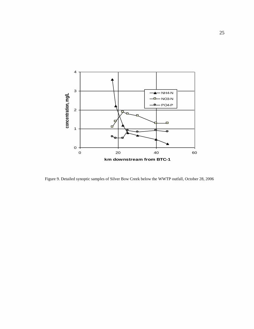
25
0
1
2
3
4
0 20 40 60
km downstream from BTC-1
conc
entr
atio
n, m
g/L NH4-N
NO3-N
PO4-P
Figure 9. Detailed synoptic samples of Silver Bow Creek below the WWTP outfall, October 28, 2006

26
0
1
2
3
4
5
6
7
0 10 20 30 40 50
co
nc
en
tra
tio
n, m
g/L
km downstream from BTC-1
NH4-N
NO3-N
PO4-P
Up
pe
r site
s fr
oze
n
0
2
4
6
8
10
12
14
0 10 20 30 40 50
loa
d, k
g/h
ou
r
km downstream of BTC-1
NH4-N
NO3-N
PO4-P
Up
per sites
froze
n
Lower sites frozen
Figure 10. Synoptic samples December 18, 2006

27
0
1
2
3
4
5
6
7
8
9
0 10 20 30 40
co
nc
en
tra
tio
n, m
g/L
km downstream from BTC-1
NH4-N
NO3-N
PO4-P
Up
pe
r site
s fro
ze
n
0
2
4
6
8
10
12
14
0 10 20 30 40
loa
d, k
g/h
ou
r
km downstream of BTC-1
NH4-N
NO3-N
PO4-P
Up
pe
r site
s fro
ze
n
Lower sites frozen or partially frozen
Figure 11. Synoptic samples of January 29, 2007
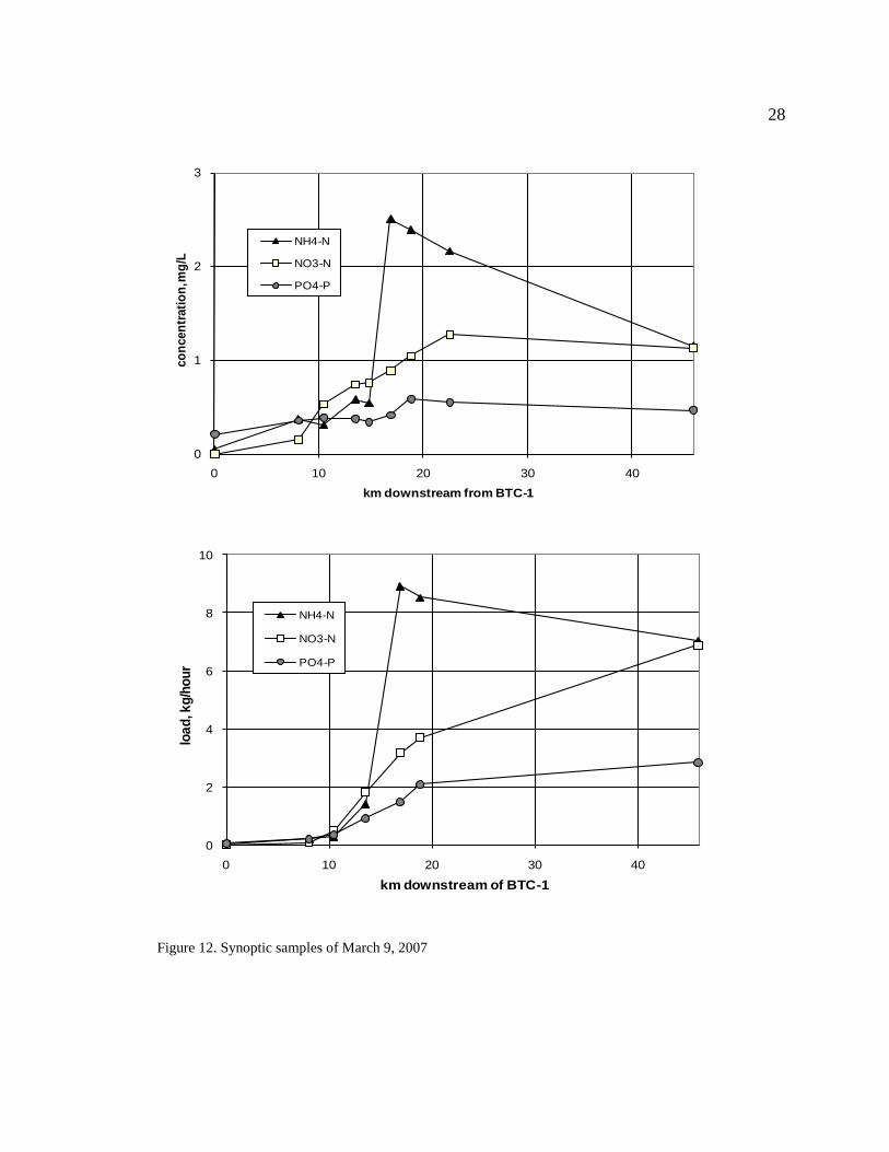
28
0
1
2
3
0 10 20 30 40
co
ncen
trati
on
, mg
/L
km downstream from BTC-1
NH4-N
NO3-N
PO4-P
0
2
4
6
8
10
0 10 20 30 40
loa
d, k
g/h
ou
r
km downstream of BTC-1
NH4-N
NO3-N
PO4-P
Figure 12. Synoptic samples of March 9, 2007
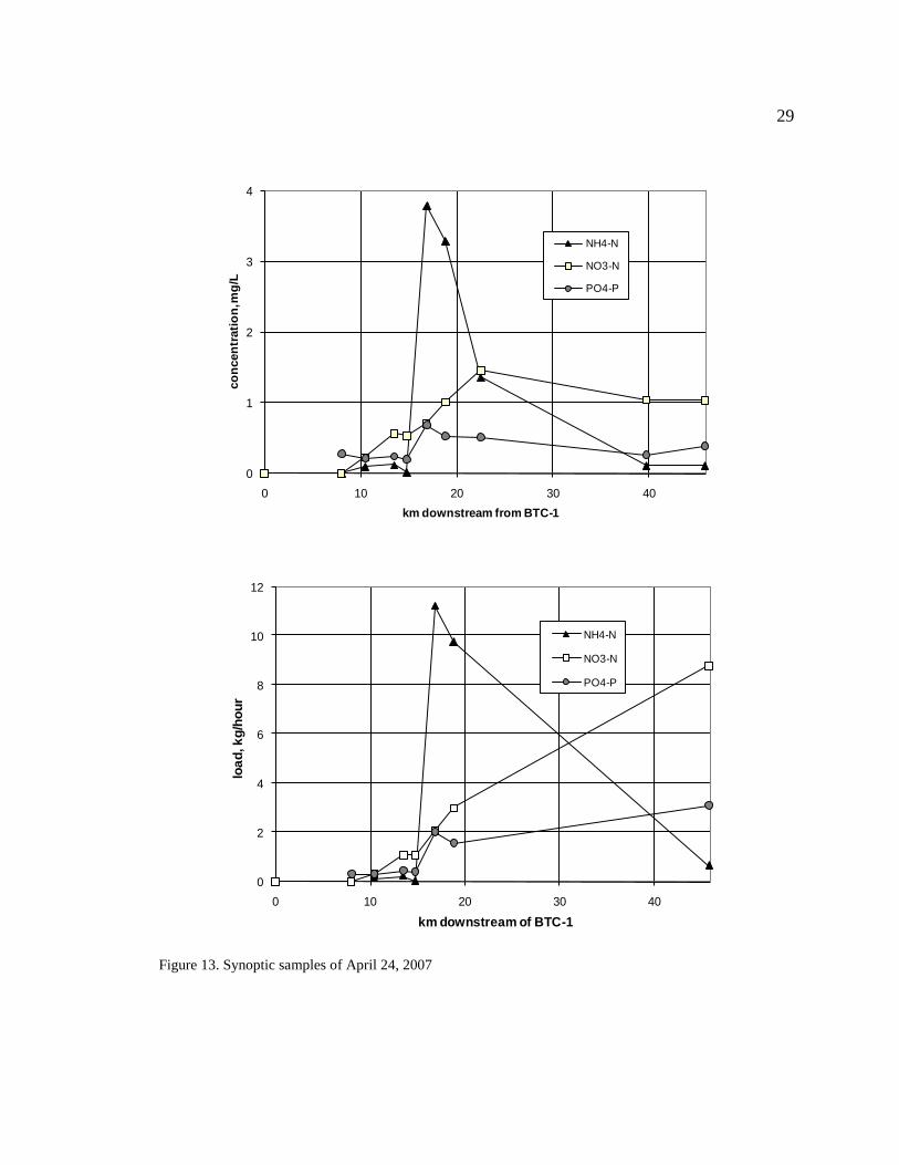
29
0
1
2
3
4
0 10 20 30 40
co
ncen
trati
on
, mg
/L
km downstream from BTC-1
NH4-N
NO3-N
PO4-P
0
2
4
6
8
10
12
0 10 20 30 40
loa
d, k
g/h
ou
r
km downstream of BTC-1
NH4-N
NO3-N
PO4-P
Figure 13. Synoptic samples of April 24, 2007

30
0
1
2
0 10 20 30 40
co
ncen
trati
on
, mg
/L
km downstream from BTC-1
NH4-N
NO3-N
PO4-P
0
2
4
6
8
0 10 20 30 40
loa
d, k
g/h
ou
r
km downstream of BTC-1
NH4-N
NO3-N
PO4-P
Figure 14. Synoptic samples of May 31, 2007

31
0
0.5
1
1.5
2
2.5
3
0 10 20 30 40 50
co
ncen
trati
on
, m
g/L
km downstream from BTC-1
NH4-N
NO3-N
PO4-P
0
2
4
6
8
10
0 10 20 30 40 50
load
, kg
/ho
ur
km downstream of BTC-1
NH4-N
NO3-N
PO4-P
Figure 15. Synoptic samples of June 19, 2007

32
0
1
2
3
4
5
0 5 10 15 20 25
km downstream from BTC-1
co
nc
en
tra
tio
n, m
g/L
NH4-N
NO3-N
PO4-P
Figure 16. Synoptic samples of July 27, 2007

33
0
1
2
3
0 10 20
co
ncen
trati
on
, mg
/L
km downstream from BTC-1
NH4-N
NO3-N
PO4-P
0
2
4
6
0 10 20
loa
d, k
g/h
ou
r
km downstream of BTC-1
NH4-N
NO3-N
PO4-P
Figure 17. Synoptic samples of August 31, 2007

34
4.1.2 Nitrate
Nitrate concentrations and loads showed a significant increase between sites
BTC-1 and BTC-4. Concentrations of dissolved nitrate exceeded 1 mg/L as N on most
sampling dates at BTC-4 and SBC-1. This has been shown in other studies (WET, 2004;
Carstarphen et al., 2004; Lafave, 2008) and been attributed to the effects of non-point
sources of nutrients as Blacktail Creek makes its way through the Butte Summit Valley.
Below station SBC-1, further additions of nitrate come from the Montana Pole and Lower
Area One (LAO) treatment facilities. The WWTP discharge adds relatively little nitrate
directly to Silver Bow Creek, since most of the nitrogen leaving the WWTP is in reduced
form as ammonium ion. However, oxidation of ammonium to nitrate is probably the
main reason for the observed increases in nitrate concentrations and loads on most dates
in Silver Bow Creek between Lower Area One and SBC-3. Because the rate of this
oxidation is slower in the cooler months, nitrate values increase more gradually
downstream of SBC-2 in winter as opposed to summer.
The above findings cast doubt on the conclusion of WET (2004) that increases in
nitrate concentration below Lower Area One are due to discharging groundwater and/or
seepage of nutrients from a nearby meat packing operation. Based on specific
conductance transects (C. Gammons, pers. commun.), it is considered unlikely that much
groundwater enters Silver Bow Creek below the Interstate 90 bridge at Lower Area One
during normal baseflow conditions.

35
4.1.3 Phosphate
Concentrations and loads of phosphate were typically low in Blacktail Creek and
upper Silver Bow Creek (at SBC-1). The confluence of the WWTP effluent caused an
abrupt increase in phosphate concentrations and loads. Below the WWTP,
concentrations of phosphate-P in Silver Bow Creek were highly elevated on all sampling
dates, falling in the range 0.3 to 1.0 mg/L as P.
4.1.4 Oxidation of ammonia to nitrate
Figure 18 shows detailed changes in the speciation of dissolved nitrogen below
the WWTP outfall, measured on samples collected August 9, 2006. The WWTP
typically discharges 3 to 10 cfs of water containing dissolved ammonium concentrations
above 10 mg/L as N. This ammonium is then oxidized by microbes to nitrite, as shown
by the following equation:
OHHNOONH2223
5.1 (1).
Microbes that oxidize ammonia to nitrite include species of the genera Nitrosomonas, and
Nitrosospira (Kowalchuk 2001). The nitrite is then further oxidized to nitrate, as shown
by the following equation:
3225.0 NOONO (2).
Bacteria that oxidize nitrite to nitrate include Nitrobacter, and Nitrospira (Kowalchuk
2001). The combination of reactions (1) and (2) result in the observed synoptic profiles
in nitrate, nitrite, and ammonia concentrations shown in Figure 18. In general, nitrite

36
concentrations are elevated until all of the ammonia is oxidized, at which point nitrite
drops to undetectable levels.
0.01
0.1
1
10
0 1 2 3 4 5 6
km below mixing zone
pp
m a
s N
nitrate
ammonia
nitrite
Figure 18. Detailed changes in speciation of nitrogen below the WWTP outfall on August 9, 2006.
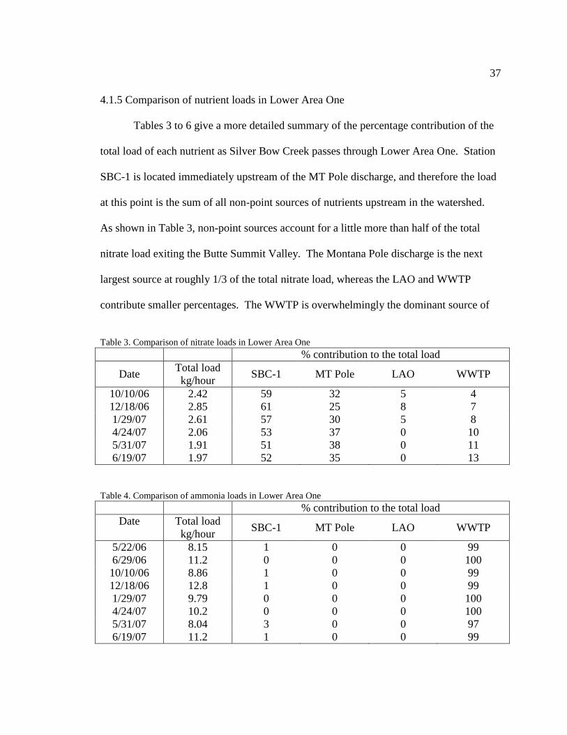
37
4.1.5 Comparison of nutrient loads in Lower Area One
Tables 3 to 6 give a more detailed summary of the percentage contribution of the
total load of each nutrient as Silver Bow Creek passes through Lower Area One. Station
SBC-1 is located immediately upstream of the MT Pole discharge, and therefore the load
at this point is the sum of all non-point sources of nutrients upstream in the watershed.
As shown in Table 3, non-point sources account for a little more than half of the total
nitrate load exiting the Butte Summit Valley. The Montana Pole discharge is the next
largest source at roughly 1/3 of the total nitrate load, whereas the LAO and WWTP
contribute smaller percentages. The WWTP is overwhelmingly the dominant source of
Table 3. Comparison of nitrate loads in Lower Area One
% contribution to the total load
Date Total load
kg/hour SBC-1 MT Pole LAO WWTP
10/10/06 2.42 59 32 5 4
12/18/06 2.85 61 25 8 7
1/29/07 2.61 57 30 5 8
4/24/07 2.06 53 37 0 10
5/31/07 1.91 51 38 0 11
6/19/07 1.97 52 35 0 13
Table 4. Comparison of ammonia loads in Lower Area One
% contribution to the total load
Date Total load
kg/hour SBC-1 MT Pole LAO WWTP
5/22/06 8.15 1 0 0 99
6/29/06 11.2 0 0 0 100
10/10/06 8.86 1 0 0 99
12/18/06 12.8 1 0 0 99
1/29/07 9.79 0 0 0 100
4/24/07 10.2 0 0 0 100
5/31/07 8.04 3 0 0 97
6/19/07 11.2 1 0 0 99

38
Table 5. Comparison of total N loads (ammonia + nitrate loads)
% contribution to the total load
Date Total load
kg/hour SBC-1 MT Pole LAO WWTP
5/22/06 10.7 11 2 3 84
6/29/06 14.1 8 4 2 87
10/10/06 11.3 14 7 1 78
12/18/06 15.6 12 5 1 82
1/29/07 12.4 12 6 1 81
4/24/07 12.2 9 6 0 84
5/31/07 10.0 12 7 0 80
6/19/07 13.1 9 5 0 86
Table 6. Comparison of phosphate loads in Lower Area One
% contribution to the total load
Date Total load
kg/hour SBC-1 MT Pole LAO WWTP
5/22/06 1.31 19 1 1 79
6/29/06 1.40 5 1 1 93
10/10/06 1.55 1 1 0 97
12/18/06 1.82 4 1 0 95
1/29/07 1.81 6 1 0 93
4/24/07 3.23 13 1 1 85
5/31/07 1.19 34 2 1 63
6/19/07 3.58 13 1 8 79
ammonia and phosphate loading (Tables 4, 6). When nitrate and ammonia are combined
(total dissolved N), the WWTP contributed > 78% of the total N load on all sampling
dates (Table 5). As mentioned above, most of the ammonia that is released by the
WWTP eventually oxidizes to nitrate. Thus, the total N load is a more useful metric then
nitrate alone to evaluate the impacts of the WWTP on nutrients in Silver Bow Creek.
4.1.6 Comparison of Nutrient Loads in Silver Bow Creek to Reference Conditions

39
To better compare the nutrient loads in Silver Bow Creek to other watersheds
nationwide, the average annual load exiting the Butte Summit Valley was divided by the
drainage area of the basin (103 sq. miles) and then converted to metric units to calculate
the “nutrient yield” (kg/km2/year). This was compared to the average runoff (cm/year),
which was taken as the average discharge at USGS gaging station 12323250 over the
entire 2006 and 2007 calendar years divided by the area of the watershed. Figure 19
shows how Silver Bow Creek compares with reference conditions established for U.S.
rivers in “developed” and “undeveloped” basins (Smith et al. 2003). The results show
that the N and P yields for Silver Bow Creek plot well above the national trends for
“developed” basins. However, if the effects of the WWTP were removed Butte Summit
Valley would have nutrient loads below the national average yields of other developed
basins. This is an important result, and underscores the need to improve nutrient removal
in the Butte Silver Bow wastewater treatment plant to restore Silver Bow Creek to a more
natural condition. Of course, any new upgrades to the treatment plant are unlikely to
remove 100% of the nutrient load. However, even if nutrient removal were 80-90%, this
would go a long ways to improving the eutrophication problem in Silver Bow Creek

40
0.1
1
10
100
1000
10000
0.01 0.1 1 10 100 1000
Runoff, cm/yr
N Y
ield
, k
g/k
m2/y
r
U.S. Developed Basins
U.S. Reference Basins
A.
0.01
0.1
1
10
100
1000
0.01 0.1 1 10 100 1000
Runoff, cm/yr
P Y
ield
, kg
/km
2/y
r
SBC with WWTP SBC without WWTP
U.S. Developed Basins
U.S. Reference Basins
B.
Figure 19. Comparison of estimated annual N and P yield from Silver Bow Creek with national average for
developed and reference basins (from Smith et al., 2003)

41
4.2 Diurnal sampling
4.2.1 Diurnal nutrient sampling of July, 2006
On July 11-12, 2006, a set of diurnal samples was taken at three locations (SBC-
1B, WWTP, and SBC-3) to see how the nutrient levels changed throughout the day.
Although the data are scattered, there appears to have been an increase in nitrate
concentrations during the night at SBC-1B, which is above the WWTP outfall. Previous
studies have shown that dissolved nitrate concentrations have a tendency to increase at
night in streams in the upper Clark Fork River basin (Brick and Moore, 1996; Gammons
et al., 2007; Parker et al., 2007), and elsewhere (Scholefield et al., 2005) although the
reasons why are not known with confidence. Neither ammonia nor nitrite followed a
clear diurnal pattern at SBC-1B, although there is a possible trend to higher
concentrations during the day (Figure 20). The single very high nitrite value at 13:00
may have been an error.

42
0
0.5
1
1.5
2
2.5
3
8:30 14:30 20:30 2:30 8:30
mg
/L N
O3
- -N,
NH
4+-N
0.000
0.005
0.010
0.015
0.020
0.025
0.030
0.035
0.040
0.045
0.050
mg
/L N
O2
- -N
NO3-N
NH4-N
NO2-N
Figure 20. Diurnal changes in nutrients at SBC-1B
The concentrations of nutrients in the WWTP outfall showed quite a bit of
variation over the 24-h period (Fig. 21), but the changes didn‟t follow a clear diurnal
pattern. Concentrations of ammonia-N were much higher than nitrate-N at all times of
the day, although there is a possible trend of higher ammonia/nitrate ratios at night and
lower ratios during the day. This could reflect a more rapid rate of oxidation of ammonia
to nitrate during the warm daylight hours. Concentrations of nitrite also increased at
night, relative to daytime.

43
0
5
10
15
20
25
30
8:30 14:30 20:30 2:30 8:30
mg
/L N
H4+-N
0
0.2
0.4
0.6
0.8
1
1.2
1.4
mg
/L N
O3
- -N,
NO
2- -N
NH4-N
NO3-N
NO2-N
Figure 21. Diurnal changes in nutrients at the WWTP outfall.
More systematic diurnal changes in nutrient concentration were noted at SBC-3
compared to the other stations (Fig. 22). Concentrations of ammonia and nitrite
increased at night, and decreased during the day, whereas nitrate followed the reverse
pattern. These diel patterns are due to the biological activity in the water, which is
dependent on both sunlight and temperature. During the day when the water
temperatures are higher and dissolved oxygen is being produced by photosynresearch, the
ammonia oxidizes faster. This causes the ammonia concentrations to be lower during the
day and higher at night. Since ammonia oxidizes to nitrate, the concentrations of nitrate
vary in an inverse fashion to those of ammonia. Overall the diurnal trends in nitrite
appear to follow ammonia closer than nitrate, although the correlation isn‟t perfect.

44
0
0.5
1
1.5
2
2.5
3
3.5
4
8:30 14:30 20:30 2:30 8:30
mg
/L N
O3
- -N, N
H4+-N
0
0.05
0.1
0.15
0.2
0.25
0.3
0.35
0.4
mg
/L N
O2
- -N
NO3-N
NH4-N
NO2-N
Figure 22. Diurnal changes in nutrients at SBC-3.
Based on the preliminary data collected in this research, it is clear that
concentrations of ammonia and nitrate in Silver Bow Creek change depending on the
time of day. These changes are more noticeable below the WWTP outfall as compared to
above the outfall. More detailed investigations of diurnal nutrient cycling in Silver Bow
Creek are in progress (Babcock and Gammons, 2008; Babcock, in preparation).
45
4.2.2 Dissolved Oxygen Concentrations and the Silver Bow Creek “Dead Zone”
On August 6, 2006, starting at 4:00 a.m. and ending around 6:00 a.m., DO
concentrations were taken at 8 locations along Silver Bow Creek in the pre-dawn hours.
The results (Fig. 23) show that DO values above the WWTP were near 8 mg/L in the pre-
dawn hours. However, the DO concentrations for all stations below the WWTP fell
below 5 mg/L, with the most severe DO depletions (< 2 mg/L) at the SBC-3 and “Town
Pump” monitoring sites. These unusually low DO concentrations are believed to be
caused by the oxidation of ammonia from the WWTP in the absence of photosynresearch
(e.g., see Dunnette and Avedovech, 1983). The reach of critically low DO concentrations
is denoted the “Dead Zone” in Figure 23. This term is often used to describe hyper-
eutrophic waters, including ocean waters such as the northern Gulf of Mexico (Malakoff,
1998; Dodds, 2006), that show extreme hypoxia during certain times of the year. In the
middle part of the Silver Bow Creek Dead Zone, concentrations of DO clearly dropped to
levels that would be lethal to trout on the morning of August 6, 2006.
To further investigate the extent of the Silver Bow Creek Dead Zone, 24-h
changes in dissolved oxygen concentration were measured at 6 locations above and
below the WWTP outfall on August 14-17, 2006 (Figure 24). The DO profile above the
WWTP showed higher DO concentrations during the daytime and lower concentrations
at night, as expected, although the levels stayed above the aquatic life standard of 5 mg/L
over the entire 24 hour period. The WWTP outlet had a fairly steady DO concentration
around 4 mg/L, indicating O2 consumption. This value was also close to the DO levels
measured at the WWTP outfall during each monthly visit (see data in Appendix A1).

46
0
2
4
6
8
10
mg
/L D
O
Silver Bow CreekSto
rm D
rain
Butte
WWTP
1515
9090
1515
5 ppm
Dead ZoneDead ZoneDead Zone
SBC-1B
Figure 23. Dissolved oxygen concentrations in Silver Bow Creek in the pre-dawn hours of August 6, 2006
Monitoring stations in Silver Bow Creek below the WWTP clearly showed the serious
impacts of the sewage treatment outfall. At SBC-2, DO concentrations dropped below 4
mg/L during both nights (Fig. 24). At SBC-3, DO concentrations dropped below 1 mg/L
for roughly 10 hours during the late afternoon and nighttime period. At the Town Pump
site, nighttime O2 concentrations dropped below 2 mg/L. By the time the stream got to
the Nissler site, most of the ammonia was probably already oxidized, and therefore the
nighttime depletion in O2 was less extreme. Nonetheless, Figure 24 shows that O2 levels
dropped below 4 mg/L at Nissler for over 6 hours. At Nissler, all three datasondes were
placed in the water side-by-side over the 24 hour sampling period. Figure 24 shows how
well their DO profiles matched.
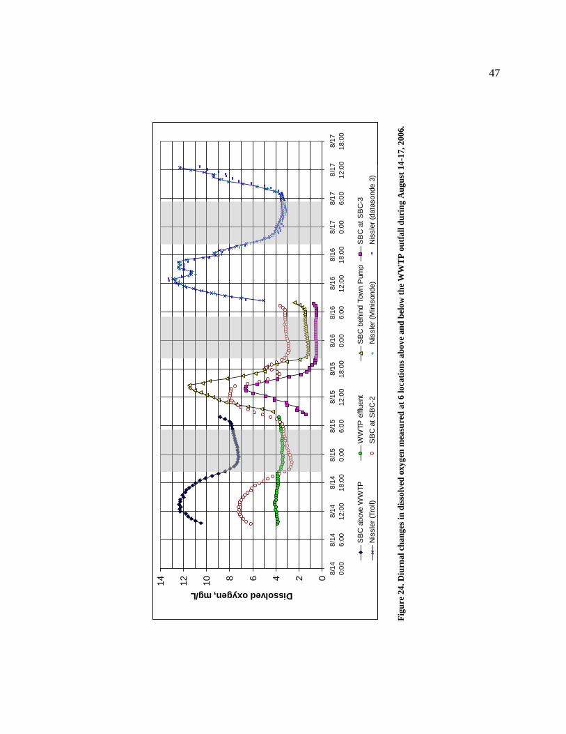
47
02468
10
12
14
8/1
4
0:0
0
8/1
4
6:0
0
8/1
4
12
:00
8/1
4
18
:00
8/1
5
0:0
0
8/1
5
6:0
0
8/1
5
12
:00
8/1
5
18
:00
8/1
6
0:0
0
8/1
6
6:0
0
8/1
6
12
:00
8/1
6
18
:00
8/1
7
0:0
0
8/1
7
6:0
0
8/1
7
12
:00
8/1
7
18
:00
Dissolved oxygen, mg/L
SB
C a
bove
WW
TP
WW
TP
effl
uent
SB
C b
ehin
d T
ow
n P
um
pS
BC
at
SB
C-3
Nis
sle
r (T
roll)
SB
C a
t S
BC
-2N
issle
r (M
inis
onde)
Nis
sle
r (d
ata
sonde 3
)
Fig
ure
24
. D
iurn
al
cha
ng
es i
n d
isso
lved
oxy
gen
mea
sure
d a
t 6
lo
ca
tio
ns
ab
ov
e an
d b
elo
w t
he
WW
TP
ou
tfa
ll d
uri
ng
Au
gu
st 1
4-1
7,
20
06.

48
4.2 Stable isotopes
The results of stable isotope analysis of samples collected in this research during
October 2006 and June 2007 are summarized in Table 7 and Figure 25. The 2006
samples were collected at the same time as the synoptic nutrient sampling of 10/10/06.
Table 7. Stable isotope results
Location Sample Date δ15
N-NO3 δ18
O-NO3 δ15
N-NH4
Samples from October, 2006
MT Pole 10/10/06 12.1 0.7 n.a.
LAO 10/10/06 9.9 10.0 n.a.
WWTP 10/10/06 n.a. n.a. 10.1 (7.6)
SBC-1 10/10/06 10.5 -1.2 n.a.
SBC-3 10/10/06 5.0 (5.3) 1 -2.4 (-1.9)
1 16.5 (14.9)
1
Samples from June, 2007
MT Pole 6/26/07 12.7 (12.3) 1
2.0 n.a.
SBC-1 6/26/07 11.2 3.2 n.a.
SBC-2 6/28/07 8.6 5.4 n.a.
SBC-2B2 6/28/07 7.9 1.7 n.a.
SBC-3 6/28/07 7.8 -3.0 n.a.
Town Pump 6/28/07 8.3 -5.0 n.a.
Nissler 6/28/07 11.4 -5.4 n.a. 1 Values in parentheses are laboratory duplicates.
2 SBC-2B is located mid-way
between SBC-2 and SBC-3. n.a. = not analyzed.
Supporting field and nutrient concentration data for the 2007 isotope samples are given in
Table A1 of the Appendix.
As shown in Figure 25, the stable isotopic compositions of nitrate from the
various waters sampled in this study are similar to those collected by previous workers
for shallow alluvial groundwater wells in the Butte Summit Valley. As discussed by
LaFave (2008), the range in isotopic composition for nitrate in Summit Valley
groundwater is most consistent with derivation of N from human or animal waste,
although lesser contributions from other sources (such as chemical fertilizer, munitions,
or acid rain) cannot be discounted. Ammonium from the WWTP shows an N-isotope

49
composition within the ranges of δ15
N-NO3 from the groundwater wells and Silver Bow
Creek samples and therefore cannot be used to differentiate the WWTP from other
nitrogen sources.
15N-nitrate, ‰
-5 0 5 10 15 20 25 30 35
18O
nitra
te,
‰
-20
-15
-10
-5
0
5
10
15
20
25
GW wells, HKM
GW wells, MBMG
Silver Bow Creek
Montana Pole
LAO
SBC water
air
SBC-3 DO
WWTP ammonia
SBC-3 ammonia
denitrification trend
chemicalfertilizers
range in predicted 18
Onitrate
from in-stream oxidation of ammonia
NO3
NH4-NO3
NH4
Figure 24. Stable isotope composition of nitrate from Silver Bow Creek compared to other results. The
green-hatched boxes show the isotopic composition of nitrate that would be obtained after leaching and
oxidation of synthetic NO3, synthetic NH4, or a 1:1 mixt
Nitrate from the MT Pole effluent is isotopically enriched in δ15
N relative to the
rest of the samples, and this may reflect denitrification of nitrate in the anaerobic plume
at Montana Pole. The line labeled “denitrification trend” in Figure 25 shows the
predicted pathway that residual nitrate would take during microbial denitrification
(reduction of NO3- to N2). This is a slope of 1:2 on the graph (Böttcher et al., 1990).
50
Overall, isotopic evidence for denitrification is weak for the groundwater and surface
waters sampled in this study, even for Montana Pole.
None of the samples, with one possible exception, plot in the boxes for synthetic
(chemical) fertilizer. The exception is a Montana Pole groundwater monitoring well
collected by MBMG. The reason that there are 3 boxes for chemical fertilizer is that the
source of the fertilizer could be nitrate, ammonium-nitrate, or ammonium. Synthetic
nitrate always has δ18
O-nitrate close to δ18
O-air, which is near +23 ‰ (Kroopnik and
Craig, 1972). If synthetic ammonium was the fertilizer source used, then oxidation of
this ammonium after application would result in nitrate that has 1/3 of its O from air, and
2/3 from water. This is because, in the microbial oxidation of ammonium to nitrate, two
O atoms come from water and one from air (Wassenaar, 1995; Clark and Fritz, 1997;
Kendall and Aravena, 2000). Stream water in Butte is isotopically light, and has an
average δ18
O value near -17 ‰ (Gammons et al., 2006). The central position of the box
labeled “NH4” was thus calculated by mass balance: 2/3*-17‰ (water) + 1/3*23‰ (air)
= -3.7 ‰. For a mixed ammonium-nitrate fertilizer, 2/3rd
‟s of the O atoms in the final
nitrate would be inherited from air, and 1/3 from local water, resulting in a predicted
δ18
O-nitrate value of +9.7 ‰.
SBC-3 ammonia is highly enriched in 15
N compared to ammonia coming from the
WWTP outfall: the δ15
N-NH4 values are +16‰ and +8‰, respectively (Table 7). The
enrichment in 15
N with distance downstream may be due to preferential oxidation of
isotopically-light ammonium by microbes such as Nitrosomonas sp., leaving isotopically
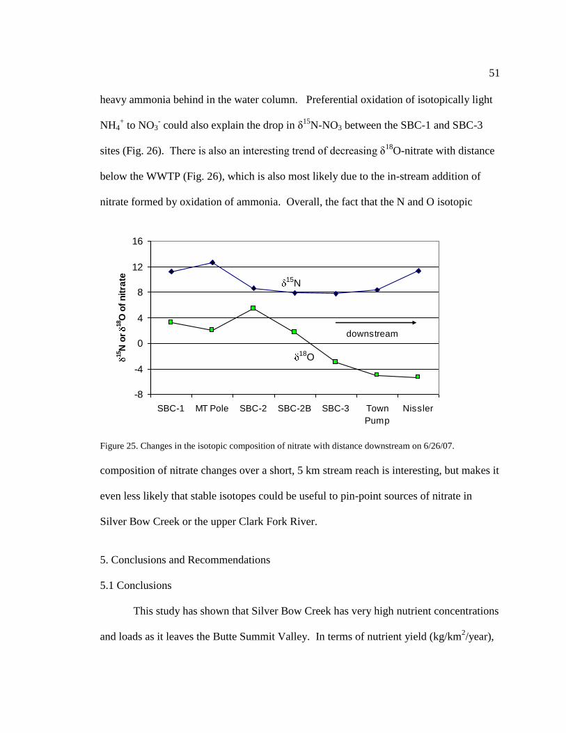
51
heavy ammonia behind in the water column. Preferential oxidation of isotopically light
NH4+ to NO3
- could also explain the drop in δ
15N-NO3 between the SBC-1 and SBC-3
sites (Fig. 26). There is also an interesting trend of decreasing δ18
O-nitrate with distance
below the WWTP (Fig. 26), which is also most likely due to the in-stream addition of
nitrate formed by oxidation of ammonia. Overall, the fact that the N and O isotopic
-8
-4
0
4
8
12
16
SBC-1 MT Pole SBC-2 SBC-2B SBC-3 Town
Pump
Nissler
15N
or
18O
of
nit
rate 15N
18O
downstream
Figure 25. Changes in the isotopic composition of nitrate with distance downstream on 6/26/07.
composition of nitrate changes over a short, 5 km stream reach is interesting, but makes it
even less likely that stable isotopes could be useful to pin-point sources of nitrate in
Silver Bow Creek or the upper Clark Fork River.
5. Conclusions and Recommendations
5.1 Conclusions
This study has shown that Silver Bow Creek has very high nutrient concentrations
and loads as it leaves the Butte Summit Valley. In terms of nutrient yield (kg/km2/year),

52
the amount of N and P leaving the watershed is far in excess of average national trends
for “developed basins” (Smith et al., 2003). The largest source of nutrient contamination
is the Butte wastewater treatment plant (WWTP), which contributes over 80% and 60%
of the total N and total P loads, respectively, during normal baseflow conditions. When
the contribution from the WWTP is removed, Silver Bow Creek has a nutrient yield more
consistent with national averages for developed basins. Besides the WWTP, significant
loads of nitrate and phosphate in upper Silver Bow Creek come from non-point sources in
the Butte Summit Valley, as well as discharges of groundwater from the Montana Pole
and Lower Area One treatment plants.
Most of the N exiting the WWTP is in the form of ammonium (NH4+). The
ammonium is then oxidized to nitrate by bacteria as the water moves downstream, and
this oxidation reaction occurs faster when the temperature is warmer. Since the rate of
oxidation is temperature dependent, both seasonal and diurnal fluctuations occur in
ammonia and nitrate concentrations in Silver Bow Creek. Oxidation of ammonia to
nitrate also results in downstream increases in nitrate concentrations and loads. These
should not be misinterpreted as being due to the influx of nitrate-rich groundwater.
During mid-summer, low-flow conditions, dissolved oxygen concentrations in
Silver Bow Creek below the WWTP drop below 2 mg/L during the night, creating a
“dead zone” where aquatic life is severely impaired. Oxidation of ammonium is believed
to be the main source of this extreme depletion in dissolved oxygen. Besides playing a
dominant role in consumption of dissolved oxygen, concentrations of ammonium in
53
Silver Bow Creek below WWTP are sometimes high enough to be toxic to aquatic life
based on current EPA standards.
The stable isotopic composition of nitrate and ammonium in Silver Bow Creek is
most consistent with derivation from human and animal waste. With the possible
exception of the discharge pipe from the Montana Pole plant, none of the waters sampled
show clear isotopic evidence for denitrification. Below the WWTP outfall, oxidation of
ammonium to nitrate results in significant changes in the O and N isotopic composition
of nitrate, making it difficult if not impossible to use stable isotopes to discriminate
between multiple sources of N contamination to the watershed.
5.2. Recommendations
Based on this study, it is clear that improvements should be made to the Butte-
Silver Bow wastewater treatment plant to remove N and P prior to discharge to Silver
Bow Creek. The “dead zone” between Butte and Rocker will most likely return each
summer so long as current conditions prevail. As well, nutrient loads from the WWTP
create a large crop of biomass (aquatic plants and algae) in the stream that is further
evidence of hyper-eutrophic conditions. If improvements are made to the WWTP,
nutrient loads in SBC would be much closer to nation-wide reference conditions for
developed watersheds.
Future nutrient monitoring efforts in upper Silver Bow Creek should include both
ammonia-N and nitrate-N. Apparent increases in nitrate concentration and load in Silver
Bow Creek between the WWTP outfall and the town of Rocker are likely due to
54
oxidation of ammonia, not to the input of nitrate from groundwater or additional off-
stream sources. Future nutrient monitoring should also take diurnal cycling into account,
especially below the WWTP outfall. Concentrations measured depends on the time of
day. This is especially true for dissolved oxygen and the nitrogen compounds (nitrate
and ammonium).
The USGS monitoring station below the WWTP is not a good place to collect water
quality samples because Silver Bow Creek is poorly mixed at this location. Samplers
need to take care to collect width- and depth-integrated samples to obtain a representative
bulk sample. Better yet, it is recommended to move the water quality collection point to
the first frontage road bridge, roughly 0.6 km downstream (SBC-2 of this study).
All of the data in this research were collected during baseflow-to-moderately high
flow conditions. Additional studies should be undertaken to look at loads and
concentrations of nutrients exiting Butte during Spring runoff and storm events. For
example, it is possible that there is a flush of nutrients off Butte Hill during storms, some
of which is incompletely processed through the WWTP, and some of which enters
directly into the streams.
Based on the results of this research, it seems unlikely that stable isotopes of N can
be used to pinpoint sources of N-contamination in the upper Silver Bow Creek basin.
However, this study did show interesting changes in δ18
N and δ18
O of nitrate as it passes
downstream from Butte to Rocker and beyond. Further work is recommended to
investigate the causes of these isotopic trends..

55
6.0 References
Babcock J. (in preparation) Diurnal cycling of metals and nutrients in Silver Bow Creek,
Montana. M.S. Research, Montana Tech of The University of Montana.
Babcock J. and Gammons C.H. (2008) Diurnal cycling of nutrients in a hyper-eutrophic
stream: Silver Bow Creek, Montana. Proc. 2008 Montana Water Center Conference,
http://www.awra.org/state/montana/pdfs/2008_proceedings_screen.pdf
Bohlke J.K. and Denver J.M. (1996) Combined use of groundwater dating, chemical, and
isotopic analysis to resolve the history and fate of nitrate contamination in two
agricultural watersheds, Atlantic Costal Plain, Maryland: Water Resources Research
31, 2319-2339.
Böttcher J., Strebel O., Voerkelius S. and Schmidt H. L. (1990) Using isotope
fractionation of nitrate-nitrogen and nitrate-oxygen for evaluation of microbial
denitrification in a sandy aquifer. Journal of Hydrology 114, 413-424.
Botz M. K. (1969) Hydrogeology of the upper Silver Bow Creek drainage area, Montana.
Montana Bureau of Mines and Geology, Bulletin 75, 32 pp.
Brick C. M. and Moore J. N. (1996) Diel variation of trace metals in the upper Clark Fork
River, Montana. Envir. Sci. Technol. 30, 1953-1960.
Carstarphen C.A., LaFave, J.I., and Patton, T.W. (2004) Water levels and nitrate in
Warne Heights, upper Summit Valley, Silver Bow County, Montana, Mont. Bur.
Mines Geol. Ground-water Open-File Report 18, 52 pp.

56
Clark I. and Fritz P., 1997. Environmental Isotopes in Hydrogeology. Lewis Pub., New
York.
Coplen T. B. (1993) Use of environmental isotopes, in Alley, W.A., ed, Regional
Ground-Water Quality: New York, Van Nostrand Reinhold, Chap. 10, p. 227-254.
Deutsch B., Liskow I., Kahle P. and Voss M. (2005) Variations in the 15
N and 18
O
values of nitrate in drainage water of two fertilized fields in Mecklenburg-
Vorpommern (Germany). Aquatic Sciences 67, 156-165.
Dodds W.K. (2006) Nutrients and the “dead zone”: the link between nutrient ratios and
dissolved oxygen in the northern Gulf of Mexico. Frontiers in Ecology and the
Environment 4(4), 211-217.
Dodds W.K., Smith V.H., and Zander B. (1997) Developing nutrient targets to control
benthic chlorophyll levels in streams: A case study of the Clark Fork River. Water
Research 31, 1738-1750.
Dunnette D.A. and Avedovech R.M. (1983) Effect of an industrial ammonia discharge on
the dissolved oxygen regime of the Willamette River, Oregon. Water Research 17,
997-1007.
EPA (1999) 1999 Update of ambient water quality criteria for ammonia. U.S.
Environmental Protection Agency, Document EPA-822-R-99-014, 153 pp.
Forsell, R. (2006) “Fish in Silver Bow Creek”. Montana Standard. October 14, 2006.
Frandsen A. (2006) Mining megasite cleanup. The Water Report, Envirotech Publ,
Eugene OR, v. 26, 10-25.
57
Gammons C. H., Poulson S. R., Pellicori D. A., Roesler A., Reed P. J., Petrescu E. M.
(2006) The hydrogen and oxygen isotopic composition of precipitation, evaporated
mine water, and river water in Montana, USA. Journal of Hydrology 328, 319-330.
Gammons C.H., Grant T.M., Nimick D.A., Parker S.R., and DeGrandpre M.D. (2007)
Diel changes in water chemistry in an arsenic-rich stream and treatment-pond system.
Science of the Total Environment 384, 433-451.
GWIC (2008) Ground Water Information Center. Montana Bureau of Mines and
Geology, http://mbmggwic.mtech.edu/
Kellman, L.M. and Hillaire-Marcel, C. (2003) Evaluation of nitrogen isotopes as
indicators of nitrate contamination sources in an agricultural watershed. Agriculture,
Ecosystems and the Environment 95, p. 87-102.
Kendall C. (1998) Tracing nitrogen sources and cycles in catchments. In: C. Kendall and
J. J. McDonnell (eds.), Isotope Tracers in Catchment Hydrology. Elsevier,
Amsterdam, pp. 519–576.
Kendall, C.A. and Aravena, R. (2000) Nitrate isotopes in groundwater systems, in Cook,
P.G. and Herczeg, A.L eds, Environmental Tracers in Subsurface Hydrology: Boston,
Kluwer Academic Publishers, Chap. P, p. 261 – 298.
Kowalchuk, G.A. and Stephen, J. (2001) Ammonia-Oxidizing Bacteria: A Model for
Molecular Microbial Ecology. Annu. Rev. Microbiol 55: 485-529.
Kroopnik P.M. and Craig H. C. (1972) Atmospheric oxygen: Isotopic composition and
solubility fractionation. Science 175, 54-55.

58
LaFave J. (2008) Nitrate in the ground water and surface water of the Summit Valley
near Butte, Montana. Montana Bureau of Mines and Geology, Ground-Water Open
File Report 22, 26pp.
Malakoff D. (1998) Death by suffocation in the Gulf of Mexico. Science 281, 190-192.
MDEQ (2006) Monitoring report for 2005: Streamside Tailings Operable Unit, Silver
Bow Creek/Butte Area NPL Site. Montana Department of Environmental Quality,
Helena, MT, 139 pp.
Moore J.N. and Luoma S.N. (1990) Hazardous wastes from large-scale metal extraction.
Environmental Science and Technology 24, 1279-1285.
Mueller D. K. and Helsel D. R. (1996) Nutrients in the nation‟s waters too much of a
good thing? U.S. Geological Survey, Circular 1136, 24 p.
Parker S. R., Gammons C. H., Poulson S. R., and DeGrandpre M. D. (2007) Diel changes
in pH, dissolved oxygen, nutrients, trace elements, and the isotopic composition of
dissolved inorganic carbon in the upper Clark Fork River, Montana, USA. Applied
Geochemistry 22, 1329-1343.
Pioneer Technical (2005) Warm Springs Ponds five-year review report. Pioneer
Technical Services, Inc., Butte, Montana, 40 pp. plus figures.
Redfield A.C. (1958) The biologic control of chemical factors in the environment.
American Scientist 64, 205-221.
Scholefield D., Le Goff, T., Braven J., Ebdon L., Long T., and Butler M. (2005)
Concerted diurnal patterns in riverine nutrient concentrations and physical conditions.
Science of the Total Environment 344, 201-210.

59
Smith R.A., Alexander R.B., and Schwarz G.E. (2003) Natural background
concentrations of nutrients in streams and rivers of the conterminous United States.
Environmental Science and Technology 37, 3039-3047.
TSWQC (2005) Status Report: The Clark Fork River Voluntary Nutrient Reduction
Program, 2002-2005. Document available online at the following Tri-State Water
Quality Council website: http://www.tristatecouncil.org/documents/05vnrp_eval.pdf.
TSWQC (2007) Clark Fork-Pend Oreille Watershed Management Plan: Management
Strategies for the Next Decade: 2007-2017. Document available online at the
following Tri-State Water Quality Council website:
http://www.tristatecouncil.org/documents/07cfpo_wmplan_000.pdf
Wassenaar L.I. (1995) Evaluation of the origin and fate of nitrate in the Abbotsford
Aquifer using the isotopes of 15
N and 18
O in NO3-. Applied Geochemistry 10, 391-
405.
Watson, V. and Gestring, B. (1996) Monitoring algae levels in the Clark Fork River.
Intermountain Journal of Sciences. 2:2, 17-26.
WET (2004) Nutrient source assessment, Upper Silver Bow Creek watershed. Water &
Environmental Technologies (WET). Available online at:
http://www.tristatecouncil.org/documents/04ucf_goal1.pdf.
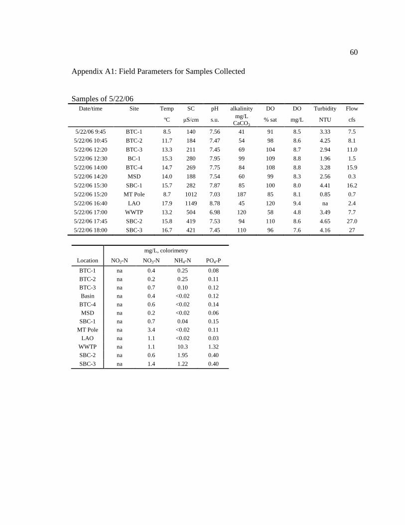
60
Appendix A1: Field Parameters for Samples Collected
Samples of 5/22/06
Date/time Site Temp SC pH alkalinity DO DO Turbidity Flow
ºC μS/cm s.u. mg/L
CaCO3 % sat mg/L NTU cfs
5/22/06 9:45 BTC-1 8.5 140 7.56 41 91 8.5 3.33 7.5
5/22/06 10:45 BTC-2 11.7 184 7.47 54 98 8.6 4.25 8.1
5/22/06 12:20 BTC-3 13.3 211 7.45 69 104 8.7 2.94 11.0
5/22/06 12:30 BC-1 15.3 280 7.95 99 109 8.8 1.96 1.5
5/22/06 14:00 BTC-4 14.7 269 7.75 84 108 8.8 3.28 15.9
5/22/06 14:20 MSD 14.0 188 7.54 60 99 8.3 2.56 0.3
5/22/06 15:30 SBC-1 15.7 282 7.87 85 100 8.0 4.41 16.2
5/22/06 15:20 MT Pole 8.7 1012 7.03 187 85 8.1 0.85 0.7
5/22/06 16:40 LAO 17.9 1149 8.78 45 120 9.4 na 2.4
5/22/06 17:00 WWTP 13.2 504 6.98 120 58 4.8 3.49 7.7
5/22/06 17:45 SBC-2 15.8 419 7.53 94 110 8.6 4.65 27.0
5/22/06 18:00 SBC-3 16.7 421 7.45 110 96 7.6 4.16 27
mg/L, colorimetry
Location NO2-N NO3-N NH4-N PO4-P
BTC-1 na 0.4 0.25 0.08
BTC-2 na 0.2 0.25 0.11
BTC-3 na 0.7 0.10 0.12
Basin na 0.4 <0.02 0.12
BTC-4 na 0.6 <0.02 0.14
MSD na 0.2 <0.02 0.06
SBC-1 na 0.7 0.04 0.15
MT Pole na 3.4 <0.02 0.11
LAO na 1.1 <0.02 0.03
WWTP na 1.1 10.3 1.32
SBC-2 na 0.6 1.95 0.40
SBC-3 na 1.4 1.22 0.40

61
Samples of 6/29/2006
Date/time Site Temp SC pH alkalinity DO DO Turbidity Flow
ºC μS/cm s.u. mg/L
CaCO3 % sat mg/L NTU cfs
6/29/06 16:10 BTC-1 13.8 163 7.87 56 98 8.1 4.08 5.8
6/29/06 16:50 BTC-2 na 193 7.59 na 89 7.0 7.72 na
5/22/06 15:00 BTC-3 17.9 216 7.77 74 113 8.7 5.14 11.8
5/22/06 15:20 BC-1 20.0 248 8.46 na 109 8.1 na 3.3
5/22/06 14:00 BTC-4 18.6 279 8.17 93 141 11.0 3.08 13.5
5/22/06 13:30 SBC-1 18.3 298 8.70 94 159 12.4 3.15 13.0
5/22/06 13:00 MT Pole 8.6 1035 7.20 184 98 9.5 1.15 1.1
5/22/06 10:20 LAO 20.8 1111 8.86 88 102 7.5 1.10 1.7
5/22/06 11:00 WWTP 15.6 530 7.10 145 43 3.5 3.22 11.2
5/22/06 9:20 SBC-2 16.1 475 7.61 104 105 8.6 3.68 25.9
5/22/06 8:30 SBC-3 15.2 469 7.48 98 110 9.1 2.06 21.2
mg/L colorimetry
Location NO2-N NO3-N NH4-N PO4-P
BTC-1 na 0.2 0.16 na
BTC-2 na 0.2 0.05 0.17
BTC-3 na 0.5 <0.02 0.14
Basin na 0.3 0.21 0.15
BTC-4 0.009 0.4 <0.02 0.17
SBC-1 0.046 0.8 <0.02 0.05
MT Pole na 4.6 <0.02 0.18
LAO 0.009 1.6 <0.02 0.05
WWTP 0.028 0.9 9.8 1.14
SBC-2 0.054 1.2 2.60 0.39
SBC-3 0.091 1.8 1.41 0.49

62
Samples of 10/10/06
Date/time Site Temp SC pH alkalinity DO Turbidity Flow
ºC μS/cm s.u. mg/L
CaCO3 % sat NTU cfs
10/10/06 17:00 BTC-1 3.8 197 7.57 61 99 1.60 3.1
10/10/06 16:50 BTC-2 6.5 238 7.53 64 112 2.00 1.6a
10/10/06 15:50 BTC-3 8.6 275 7.89 105 108 1.70 4.4
10/10/06 16:30 BC-1 7.8 335 7.77 112 111 0.96 0.7
10/10/06 15:30 BTC-4 9.0 349 7.41 109 113 3.30 9.8
10/10/06 15:30 MSD 7.9 465 6.85 99 108 2.15 0.5
10/10/06 14:40 SBC-1 8.2 363 7.48 110 110 6.60 10.7
10/10/06 14:20 MT Pole 9.4 1076 6.90 202 109 0.27 0.9
10/10/06 13:40 LAO 8.8 1134 8.67 35 100 0.40 1.4
10/10/06 13:16 WWTP 15.5 548 6.79 146 57 4.10 6.4
10/10/06 12:15 SBC-2 9.7 512 7.26 116 99 12.60 19.4
10/10/06 11:15 SBC-3 9.1 516 7.25 116 111 9.40 19.8
avalue in question due to very low stream velocities
mg/L, colorimetry IC-Murdock
Location NO2-N NH4-N PO4-P NO2-N NO3-N PO4-P F Cl SO4
BTC-1 0.012 0.08 0.07 <0.2 <0.13 <0.25 0.27 5.0 25.5
BTC-2 0.008 0.06 0.04 <0.2 0.24 <0.25 0.25 8.4 33.8
BTC-3 0.017 0.06 0.09 <0.2 0.80 <0.25 0.21 9.0 32.4
Basin 0.005 <0.02 0.19 <0.2 0.65 <0.25 0.24 5.7 48.0
BTC-4 0.017 0.10 0.07 <0.2 1.20 <0.25 0.30 13.8 40.1
MSD 0.016 0.12 0.05 <0.2 0.29 <0.25 0.58 11.3 110
SBC-1 0.050 0.10 0.02 <0.2 1.30 <0.25 0.36 15.3 48.7
MT Pole 0.028 0.12 0.14 <0.2 8.30 <0.25 0.48 52.2 267
LAO 0.023 <0.02 0.03 <0.2 0.89 <0.25 0.74 51.0 488
WWTP 0.044 13.4 2.31 0.24 0.16 2.10 0.23 42.5 44.5
SBC-2 0.034 5.7 0.77 <0.2 1.40 0.46 0.28 28.5 86.4
SBC-3 0.035 4.7 0.67 <0.2 1.40 0.44 0.34 28.6 86.5

63
Samples 10/28/06
Date/time Site Temp SC pH DO
ºC μS/cm s.u. % sat
10/28/06 10:50 WWTP 13.8 538 6.70 48
10/28/06 11:15 SBC-2 7.0 521 6.88 88
10/28/06 11:25 SBC-3 6.1 524 6.95 98
10/28/06 12:05 Nissler 5.7 525 7.19 110
10/28/06 12:50 MT Livestock 6.0 519 7.23 113
10/28/06 13:00 Miles Xing 5.7 553 7.13 99
10/28/06 13:45 Fairmont 5.6 491 7.55 114
10/28/06 14:00 Opportunity 6.9 484 7.55 116
mg/L, colorimetry
Location NO2-N NO3-N NH4-N PO4-P
WWTP 0.177 0.8 12.8 1.80
SBC-2 0.073 1.1 3.60 0.59
SBC-3 0.076 1.4 2.20 0.51
Nissler 0.055 1.9 1.18 0.51
MT livestock 0.045 1.8 0.79 0.92
Miles Xing 0.035 1.7 0.65 0.84
Fairmont 0.026 1.3 0.42 0.92
Opportunity 0.024 1.3 0.20 0.85

64
Samples of 12/18/06
Date/time Site Temp SC pH DO flow
ºC μS/cm s.u. % sat cfs
12/18/06 12:55 BTC-4a 1.5 340 6.63 93 9.2
12/18/06 13:35 SBC-1 -0.1 363 7.17 96 11.4
12/18/06 13:25 MT Pole 9.2 1061 6.83 109 0.9
12/18/06 14:25 LAO 1.6 1264 8.74 101 1.6
12/18/06 14:10 WWTP 9.8 554 6.96 50 7.3
12/18/06 14:45 SBC-2 2.7 520 7.10 87 21.0
12/18/06 15:00 SBC-3 1.9 500 7.23 95 21
12/18/06 15:20 Nissler -0.1 534 7.41 93 frozen
12/18/06 15:40 Miles Xing -0.2 587 7.16 88 frozen
12/19/06 12:30 Fairmont 0.0 541 7.22 108 frozen
12/19/06 12:55 Opportunity -0.1 596 7.33 111 frozen a Sites upstream of BTC-4 were frozen.
mg/L, colorimetry IC-Murdock
Location NO2-N NH4-N PO4-P NO2-N NO3-N PO4-P F Cl SO4
BTC-4 0.035 0.03 0.09 <0.06 1.5 <0.25 0.24 13.2 41.5
SBC-1 0.012 0.07 0.07 <0.06 1.5 <0.25 0.27 15.1 44.6
MT Pole 0.019 0.01 0.14 <0.3 7.6 <1.25 0.43 51.7 257
LAO 0.009 0.04 0.03 <0.6 1.4 <2.5 0.79 61.4 508
WWTP 0.164 17.1 2.32 0.22 0.25 1.9 0.22 42.6 40.3
SBC-2 0.080 5.80 0.85 <0.12 1.4 0.84 0.29 28.3 80.3
SBC-3 0.071 4.00 0.53 <0.06 1.7 0.47 0.31 26.2 81.8
Nissler 0.065 5.30 0.63 <0.12 2.0 0.56 0.31 30.2 90.3
Miles Xing 0.019 1.28 0.43 <0.06 2.0 0.34 0.49 44.8 119
Fairmont 0.015 1.49 0.41 <0.06 2.0 0.28 0.36 33.4 97.2
Opportunity 0.014 1.59 0.40 <0.06 2.3 0.27 0.43 35.1 114
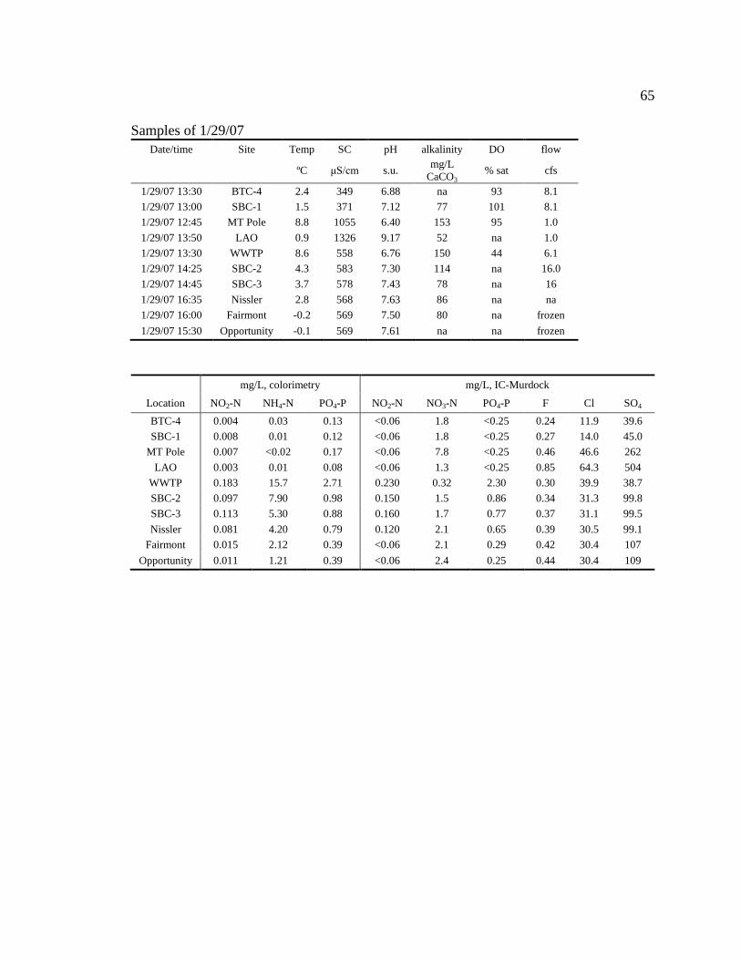
65
Samples of 1/29/07
Date/time Site Temp SC pH alkalinity DO flow
ºC μS/cm s.u. mg/L
CaCO3 % sat cfs
1/29/07 13:30 BTC-4 2.4 349 6.88 na 93 8.1
1/29/07 13:00 SBC-1 1.5 371 7.12 77 101 8.1
1/29/07 12:45 MT Pole 8.8 1055 6.40 153 95 1.0
1/29/07 13:50 LAO 0.9 1326 9.17 52 na 1.0
1/29/07 13:30 WWTP 8.6 558 6.76 150 44 6.1
1/29/07 14:25 SBC-2 4.3 583 7.30 114 na 16.0
1/29/07 14:45 SBC-3 3.7 578 7.43 78 na 16
1/29/07 16:35 Nissler 2.8 568 7.63 86 na na
1/29/07 16:00 Fairmont -0.2 569 7.50 80 na frozen
1/29/07 15:30 Opportunity -0.1 569 7.61 na na frozen
mg/L, colorimetry mg/L, IC-Murdock
Location NO2-N NH4-N PO4-P NO2-N NO3-N PO4-P F Cl SO4
BTC-4 0.004 0.03 0.13 <0.06 1.8 <0.25 0.24 11.9 39.6
SBC-1 0.008 0.01 0.12 <0.06 1.8 <0.25 0.27 14.0 45.0
MT Pole 0.007 <0.02 0.17 <0.06 7.8 <0.25 0.46 46.6 262
LAO 0.003 0.01 0.08 <0.06 1.3 <0.25 0.85 64.3 504
WWTP 0.183 15.7 2.71 0.230 0.32 2.30 0.30 39.9 38.7
SBC-2 0.097 7.90 0.98 0.150 1.5 0.86 0.34 31.3 99.8
SBC-3 0.113 5.30 0.88 0.160 1.7 0.77 0.37 31.1 99.5
Nissler 0.081 4.20 0.79 0.120 2.1 0.65 0.39 30.5 99.1
Fairmont 0.015 2.12 0.39 <0.06 2.1 0.29 0.42 30.4 107
Opportunity 0.011 1.21 0.39 <0.06 2.4 0.25 0.44 30.4 109

66
Samples of 3/9/07
Date/time Site Temp SC pH DO DO Turbidity flow
ºC μS/cm s.u. % sat mg/L NTU cfs
3/9/07 10:45 BTC-1 0.6 202 7.09 101 11.9 3.50 2.1
3/9/07 11:30 BTC-2 1.1 165 6.44 91 10.4 4.72 5.6
3/9/07 12:30 BTC-3 3.4 204 6.55 98 10.6 5.20 9.2
3/9/07 12:30 Basin 0.6 158 6.61 92 10.8 53.0 7.6
3/9/07 13:30 BTC-4 3.9 241 6.77 93 10.0 16.3 24.0
3/9/07 14:00 MT Pole 8.7 1056 6.78 120 11.0 0.75 1.0
3/9/07 14:30 SBC-1 4.2 252 6.80 96 10.2 15.5 25
3/9/07 15:10 LAO 2.5 1101 8.67 87 9.6 0.55 2.1
3/9/07 15:00 WWTP 9.1 511 6.50 55 5.1 3.70 6.5
3/9/07 15:40 SBC-2 5.6 376 7.01 92 9.4 11.5 35.0
3/9/07 15:50 SBC-3 6.2 397 6.94 98 9.8 10.0 35
3/9/07 16:20 Nissler 6.6 413 7.10 106 10.6 9.00 na
3/9/07 16:50 Opportunity na na na na na na 60.0
mg/L, colorimetery mg/L, IC-Murdock
Location NO2-N NH4-N PO4-P NO2-N NO3-N PO4-P F Cl SO4
BTC-1 0.004 0.05 0.21 <0.06 <0.13 <0.25 0.23 9.1 17.7
BTC-2 0.009 0.37 0.36 <0.06 0.16 <0.25 0.12 8.3 15.9
BTC-3 0.009 0.31 0.38 <0.06 0.53 <0.25 0.13 9.0 21.7
Basin 0.013 0.82 0.49 <0.06 <0.13 0.35 0.12 5.3 12.3
BTC-4 0.010 0.58 0.38 <0.06 0.74 <0.25 0.14 9.8 25.1
SBC-1 0.014 0.54 0.34 <0.06 0.76 <0.25 0.14 10.8 27.0
MT Pole 0.006 <0.02 0.25 <0.3 7.4 <1.25 0.46 49.0 254.9
LAO 0.010 0.04 0.16 <0.6 <1.3 <2.5 0.85 74.0 410.0
WWTP 0.173 12.1 1.99 0.25 0.63 1.20 0.44 38.8 41.6
SBC-2 0.043 2.50 0.41 0.073 0.89 0.35 0.27 21.1 53.4
SBC-3 0.056 2.39 0.58 0.076 1.0 0.36 0.31 22.5 60.3
Nissler 0.047 2.16 0.55 0.073 1.3 0.36 0.35 24.0 66.1
Opportunity 0.014 1.15 0.46 <0.06 1.1 0.28 0.34 21.0 59.3

67
Samples of 4/24/07 Date/time Site Temp SC pH DO DO Turbidity flow
ºC μS/cm s.u. % sat mg/L NTU cfs
4/24/2007 10:10 BTC-1 2.6 133 6.15 102 11.4 8.70 10.3
4/24/2007 11:00 BTC-2 7.4 175 6.61 106 11.1 4.30 11.3
4/24/2007 11:35 BTC-3 7.1 203 6.74 109 10.7 3.30 13.8
4/24/2007 12:00 BC-1 8.9 319 7.40 120 11.3 7.40 1.0
4/24/2007 12:40 BTC-4 9.5 261 7.32 129 12.1 2.40 19.0
4/24/2007 13:15 SBC-1 10.6 276 7.48 128 11.6 2.80 20.0
4/24/2007 13:10 MT Pole 8.8 1027 6.85 116 10.7 0.40 1.0
4/24/2007 14:00 LAO 10.3 1101 8.58 103 9.3 0.55 1.9
4/24/2007 13:55 WWTP 11.7 514 6.65 49 4.3 12.7 6.7
4/24/2007 14:30 SBC-2 12.5 407 7.09 107 9.3 3.70 29.0
4/24/2007 14:45 SBC-3 13.5 414 7.29 112 9.5 6.70 29
4/24/2007 15:30 Nissler 15.0 423 7.64 127 10.5 4.00 na
4/24/2007 16:00 Fairmont 12.1 400 8.24 123 11.1 na na
4/24/2007 15:20 Opportunity 11.6 399 8.65 133 12.3 na 59.0
mg/L, colorimetry mg/L, IC-Murdock
Location NO2-N NH4-N PO4-P NO2-N NO3-N PO4-P F Cl SO4
BTC-1 na na na <0.06 <0.13 <0.25 0.14 6.2 15.1
BTC -2 0.004 1.78a 0.29 <0.06 <0.13 <0.25 0.21 8.3 21.0
BTC-3 0.002 0.1 0.22 <0.06 0.2 <0.25 0.21 9.2 24.6
BC-1 na na na <0.06 0.5 <0.25 0.23 6.4 44.6
BTC-4 <.002 0.1 0.24 <0.06 0.6 <0.25 0.25 11.9 32.2
SBC-1 0.008 0.0 0.20 <0.06 0.5 <0.25 0.27 12.8 34.9
MT Pole 0.003 0.5 0.27 <0.3 7.5 <1.25 0.43 49.3 265
LAO 0.002 0.01 0.20 <0.6 <1.3 <2.5 0.88 50.4 459
WWTP 0.181 14.9 4.04 0.3 0.3 2.24 0.23 43.4 41.2
SBC-2 0.062 3.8 0.68 0.1 0.7 0.48 0.31 23.5 68.3
SBC-3 0.100 3.3 0.53 0.2 1.0 0.43 0.32 23.6 71.4
Nissler 0.098 1.36 0.52 0.2 1.5 0.37 0.35 24.5 75.2
Fairmont 0.028 0.11 0.27 <0.06 1.0 <0.25 0.31 19.2 74.3
Opportunity 0.020 0.11 0.38 <0.06 1.0 <0.25 0.33 19.3 75.5
aValue seems too high.

68
Samples of 5/31/07
Date/time Site Temp SC pH Alkalinity DO DO Turbidity flow
ºC μS/cm s.u. mg/L CaCO3 % sat mg/L NTU cfs
5/31/2007 11:45 BTC-1 8.6 137 7.15 36 na na 5.0 14.5
5/31/2007 12:15 BTC-2 11.0 181 7.09 65 107 9.6 5.9 13.8
5/31/2007 12:45 BTC-3 12.6 202 7.20 67 105 9.1 3.0 15.9
5/31/2007 13:15 BC-1 15.1 202 7.53 63 113 9.2 2.1 6.4
5/31/2007 13:45 BTC-4 15.2 236 7.52 75 117 9.5 3.6 26
5/31/2007 14:45 SBC-1 15.9 260 7.71 76 118 9.5 3.2 25.9
5/31/2007 14:29 MT Pole 8.4 1099 6.50 186 96 9.1 0.4 1.0
5/31/2007 15:30 LAO 16.0 1145 8.70 37 110 8.8 0.8 1.7
5/31/2007 15:10 WWTP 14.0 531 6.84 123 52 4.3 3.5 6.4
5/31/2007 16:00 SBC-2 17.0 376 7.28 88 94 7.4 2.3 35
5/31/2007 16:45 SBC-3 18.0 384 7.26 79 90 6.9 2.8 35
5/31/2007 17:15 Nissler 19.1 399 7.28 83 91 6.8 3.9 na
5/31/2007 17:45 Fairmont 9.6 330 7.57 88 103 9.6 6.8 na
5/31/2007 18:15 Opportunity 11.0 335 7.81 85 110 9.8 9.1 90.0
mg/L, colorimetry mg/L, IC-Murdock
Location NO2-N NH4-N PO4-P NO2-N NO3-N PO4-P F Cl SO4
BTC-1 0.002 0.09 0.12 <0.06 <0.13 <0.25 0.14 4.2 12.6
BTC-2 0.004 0.14 0.14 <0.06 <0.13 <0.25 0.23 5.9 15.4
BTC-3 0.001 0.04 0.19 <0.06 0.20 <0.25 0.22 6.6 18.2
BC-1 <.002 0.09 0.15 <0.06 <0.13 <0.25 0.14 2.2 26.7
BTC-4 0.003 0.10 0.19 <0.06 0.39 <0.25 0.23 8.0 25.3
SBC-1 0.004 0.10 0.15 <0.06 0.37 <0.25 0.26 9.0 27.9
MT Pole <.002 <0.02 0.21 <0.3 7.1 <1.25 0.44 49.8 267
LAO 0.004 <0.02 0.10 <0.6 <1.3 <2.5 0.91 46.2 445
WWTP 0.290 12.0 1.16 0.39 0.33 1.6 0.28 38.4 42.5
SBC-2 0.075 1.94 0.39 0.11 0.61 0.27 0.30 17.1 55.1
SBC-3 0.106 1.57 0.44 0.14 0.91 0.29 0.31 17.7 57.5
Nissler 0.124 1.03 0.53 0.16 1.4 0.34 0.32 18.9 60.7
Fairmont 0.020 0.08 0.30 <0.06 0.75 <0.25 0.23 10.5 50.9
Opportunity 0.014 0.01 0.24 <0.06 0.75 <0.25 0.26 10.7 53.1
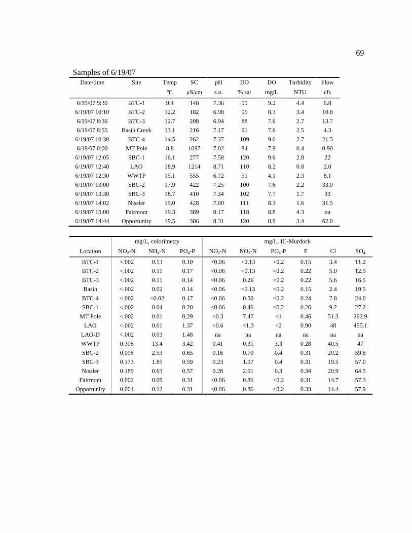
69
Samples of 6/19/07
Date/time Site Temp SC pH DO DO Turbidity Flow
ºC μS/cm s.u. % sat mg/L NTU cfs
6/19/07 9:30 BTC-1 9.4 148 7.36 99 9.2 4.4 6.8
6/19/07 10:10 BTC-2 12.2 182 6.98 95 8.3 3.4 10.8
6/19/07 8:36 BTC-3 12.7 208 6.94 88 7.6 2.7 13.7
6/19/07 8:55 Basin Creek 13.1 216 7.17 91 7.6 2.5 4.3
6/19/07 10:30 BTC-4 14.5 262 7.37 109 9.0 2.7 21.5
6/19/07 0:00 MT Pole 8.8 1097 7.02 84 7.9 0.4 0.90
6/19/07 12:05 SBC-1 16.1 277 7.58 120 9.6 2.8 22
6/19/07 12:40 LAO 18.9 1214 8.71 110 8.2 0.8 2.0
6/19/07 12:30 WWTP 15.1 555 6.72 51 4.1 2.3 8.1
6/19/07 13:00 SBC-2 17.9 422 7.25 100 7.6 2.2 33.0
6/19/07 13:30 SBC-3 18.7 410 7.34 102 7.7 1.7 33
6/19/07 14:02 Nissler 19.0 428 7.00 111 8.3 1.6 31.5
6/19/07 15:00 Fairmont 19.3 389 8.17 118 8.8 4.3 na
6/19/07 14:44 Opportunity 19.5 386 8.31 120 8.9 3.4 62.0
mg/L, colorimetry mg/L, IC-Murdock
Location NO2-N NH4-N PO4-P NO2-N NO3-N PO4-P F Cl SO4
BTC-1 <.002 0.13 0.10 <0.06 <0.13 <0.2 0.15 3.4 11.2
BTC-2 <.002 0.11 0.17 <0.06 <0.13 <0.2 0.22 5.0 12.9
BTC-3 <.002 0.11 0.14 <0.06 0.26 <0.2 0.22 5.6 16.5
Basin <.002 0.02 0.14 <0.06 <0.13 <0.2 0.15 2.4 19.5
BTC-4 <.002 <0.02 0.17 <0.06 0.50 <0.2 0.24 7.8 24.0
SBC-1 <.002 0.04 0.20 <0.06 0.46 <0.2 0.26 9.2 27.2
MT Pole <.002 0.01 0.29 <0.3 7.47 <1 0.46 51.3 262.9
LAO <.002 0.01 1.37 <0.6 <1.3 <2 0.90 48 455.1
LAO-D <.002 0.03 1.48 na na na na na na
WWTP 0.308 13.4 3.42 0.41 0.31 3.3 0.28 40.5 47
SBC-2 0.098 2.53 0.65 0.16 0.70 0.4 0.31 20.2 59.6
SBC-3 0.173 1.85 0.59 0.23 1.07 0.4 0.31 19.5 57.0
Nissler 0.189 0.63 0.57 0.28 2.01 0.3 0.34 20.9 64.5
Fairmont 0.002 0.09 0.31 <0.06 0.86 <0.2 0.31 14.7 57.3
Opportunity 0.004 0.12 0.31 <0.06 0.86 <0.2 0.33 14.4 57.9

70
Samples of 7/27/07
Date/time Site Temp SC pH DO DO Turbidity Flow
ºC μS/cm s.u. % sat mg/L NTU cfs
7/27/07 8:30 BTC-1 12.0 212 7.16 96 8.4 2.5 2.3
7/27/07 9:00 BTC-2 14.5 244 6.83 82 6.8 6.1 1.7
7/27/07 10:00 BTC-3 13.8 289 7.30 104 8.8 3.3 4.0
7/27/07 10:30 BC 13.7 352 7.77 104 8.8 4.0 0.44
7/27/07 12:00 BTC-4 17.5 354 7.72 134 10.5 1.8 9.2
7/27/07 12:20 SBC-1 18.0 394 8.16 151 11.6 2.2 9.2
7/27/07 12:18 MT Pole 9.75 1079 6.99 75 7.0 1.8 na
7/27/07 12:20 WWTP 18.4 518 6.92 56 4.3 na 7.4
7/27/07 14:00 SBC-2 20.9 559 7.77 118 8.6 na na
7/27/07 14:20 SBC-3 22.0 548 7.77 108 7.7 na na
7/27/07 15:00 Nissler 21.3 543 8.49 161 11.7 na na
mg/L, colorimetry mg/L, IC-Murdock
Location NO2-N NH4-N PO4-P NO2-N NO3-N PO4-P F Cl SO4
BTC-1 na 0.02 0.14 <0.06 <0.13 <0.2 0.29 4.1 9.6
BTC-2 na <0.02 0.13 <0.06 0.24 <0.2 0.24 6.3 18.5
BTC-3 na 0.04 0.13 <0.06 0.85 <0.2 <0.05 8.4 26.8
Basin na <0.02 0.09 <0.06 0.42 <0.2 0.21 5.7 41.0
BTC-4 na <0.02 0.12 <0.06 0.86 <0.2 <0.05 8.4 26.8
MT Pole na <0.02 0.18 <0.6 7.6 <2 <0.5 51.3 261
SBC-1 0.007 <0.02 0.16 <0.06 1.0 <0.2 0.31 15.9 41.5
WWTP 0.168 7.05 1.30 <0.06 0.15 0.68 0.28 38.2 40.8
SBC-2 0.157 3.38 0.47 <0.06 1.2 0.24 0.36 30.5 90.4
SBC-3 0.123 0.23 0.43 <0.06 4.1 0.25 0.40 30.4 94.8
Nissler 0.220 0.09 0.49 <0.06 3.1 0.27 0.45 29.3 103

71
Samples of 8/31/07
Date/time Site SC pH DO DO flow
μS/cm s.u. % sat mg/L cfs
8/30/07 13:30 BTC-1 213 8.28 82 7.1 1.3
8/30/07 14:00 BTC-2 253 8.76 62 5.2 0.61
8/30/07 15:00 BTC-3 296 8.12 90 7.6 2.6
8/30/07 14:45 BC-1 327 8.56 89 7.7 0.39
8/31/07 11:55 BTC-4 369 7.66 55 5.0 6.7
8/31/07 11:40 SBC-1 401 8.18 103 9.1 na
8/31/07 11:30 MT Pole 1033 6.90 80 7.6 na
8/31/07 12:30 WWTP 479 6.96 91 6.8 na
8/31/07 12:50 SBC-2 650 7.61 54 4.4 15
8/31/07 13:10 SBC-3 579 7.68 80 6.5 15
8/31/07 13:25 Nissler 590 8.37 64 5.3 na
HACH colorimetery IC-Murdock
Location NO2-N NH4-N PO4-P NO2-N NO3-N PO4-P F Cl SO4
BTC-1 0.003 <0.02 0.11 <0.1 <0.13 <0.1 0.35 4.3 11.8
BTC-2 0.007 <0.02 0.17 <0.1 0.27 <0.1 0.22 7.9 31.5
BTC-3 0.008 <0.02 0.16 <0.1 1.2 <0.1 0.17 9.5 33.4
Basin 0.006 <0.02 0.06 <0.1 0.30 <0.1 0.19 5.6 44.6
BTC-4 0.018 <0.02 0.18 <0.1 1.4 <0.1 0.29 15.3 37.5
SBC-1 0.0017 <0.02 0.09 <0.1 1.1 <0.1 0.37 17.6 51.1
MT Pole 0.003 <0.02 0.29 <0.5 7.7 <0.5 0.41 50.8 263.2
WWTP 0.451 7.6 1.00 0.59 1.0 0.55 0.29 38.2 40.6
SBC-2 0.261 2.7 0.85 0.32 1.6 0.23 0.43 33.9 132.3
SBC-3 0.208 0.68 0.42 0.27 3.0 0.32 0.44 33.5 131.7
Nissler
Bridge 0.007 <0.02 0.45 <0.1 2.7 0.33 0.47 32.1 147.5
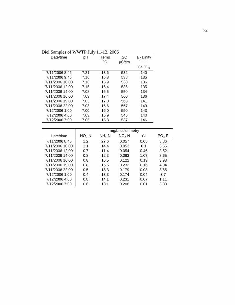
72
Diel Samples of WWTP July 11-12, 2006 Date/time pH Temp SC alkalinity
˚C μS/cmm g / L
CaCO3
7/11/2006 8:45 7.21 13.6 532 140
7/11/2006 9:45 7.16 15.8 538 135
7/11/2006 10:00 7.16 15.9 538 136
7/11/2006 12:00 7.15 16.4 536 135
7/11/2006 14:00 7.08 16.5 550 134
7/11/2006 16:00 7.09 17.4 560 136
7/11/2006 19:00 7.03 17.0 563 141
7/11/2006 22:00 7.03 16.6 557 149
7/12/2006 1:00 7.00 16.0 550 143
7/12/2006 4:00 7.03 15.9 545 140
7/12/2006 7:00 7.05 15.8 537 146
Date/time NO3-N NH4-N NO2-N Cl PO4-P
7/11/2006 8:45 1.2 27.6 0.057 0.05 3.86
7/11/2006 10:00 1.1 14.4 0.053 0.1 3.65
7/11/2006 12:00 0.7 11.4 0.054 0.46 3.52
7/11/2006 14:00 0.8 12.3 0.063 1.07 3.65
7/11/2006 16:00 0.8 16.5 0.122 0.19 3.93
7/11/2006 19:00 0.8 15.6 0.232 0.16 4.04
7/11/2006 22:00 0.5 18.3 0.179 0.08 3.65
7/12/2006 1:00 0.4 13.3 0.174 0.04 3.7
7/12/2006 4:00 0.8 14.1 0.231 0.07 1.11
7/12/2006 7:00 0.6 13.1 0.208 0.01 3.33
mg/L, colorimetry

73
Diel Samples of SBC-1B July 11-12, 2006 Date/time pH temp SC alkalinity staff gage flow
˚C μS/cmm g / L c f s
CaCO3
7/11/2006 8:30 7.9 13.6 532 95 0.69 19.1
7/11/2006 10:30 8.4 15.2 517 95 0.67 17.7
7/11/2006 12:30 8.6 17.7 508 93 0.68 18.4
7/11/2006 14:30 8.7 19.4 502 95 0.67 17.7
7/11/2006 17:00 8.7 20.8 501 91 0.67 17.7
7/11/2006 20:00 8.4 19.1 479 96 0.67 17.7
7/11/2006 23:00 7.8 17.4 514 93 0.67 17.7
7/12/2006 2:00 7.7 16.0 519 101 0.66 17.1
7/12/2006 5:00 7.7 15.0 542 97 0.62 14.4
Date/time NO3-N NH4-N NO2-N Cl2 PO4-P
7/11/2006 8:30 0.5 0.19 0.017 0.02 0.33
7/11/2006 10:30 1.5 0.19 0.017 0.50 0.32
7/11/2006 12:30 1.3 0.47 0.045 0.22 0.37
7/11/2006 14:30 1.4 0.38 0.026 0.03 0.24
7/11/2006 17:00 1.4 0.33 0.011 0.08 0.35
7/11/2006 20:00 1.2 0.09 0.006 0.02 0.31
7/11/2006 23:00 0.7 0.12 0.003 0.01 0.68
7/12/2006 2:00 1.3 0.14 0.008 0.02 0.27
7/12/2006 5:00 2.5 0.06 0.010 0.02 0.2
7/12/2006 8:00 1.4 0.16 0.012 0.01 0.33
mg/L, colorimetry

74
Diel Samples of SBC-3 July 11-12, 2006 Date/time pH temp SC DO DO alkalinity staff gage flow
˚C μS/cmp p m % s a t m g / L c f s
CaCO3
7/11/2006 9:15 7.75 14.7 522 8.6 103 94 0.46 18.2
7/11/2006 11:00 7.93 17.4 527 10.1 129 103.5 0.52 21.6
7/11/2006 13:00 7.73 19.7 517 8.8 117 NA 0.525 21.9
7/11/2006 15:00 8.11 511 10.5 144 98 0.52 21.6
7/11/2006 18:00 7.46 21.2 515 5.9 81 88 0.5 20.5
7/11/2006 21:10 7.2 18.4 523 2.53 33 95 0.51 21.0
7/11/2006 23:59 7.21 17 525 2.6 33 104 0.5 20.5
7/12/2006 3:00 7.2 15.8 526 2.4 30 106 0.49 19.9
7/12/2006 6:00 7.23 14.8 534 2.6 32 106.9 0.42 16.0
Date/time NO3-N NH4-N NO2-N Cl PO4-P
7/11/2006 9:15 3.5 1.40 0.072 0.13 1
7/11/2006 11:00 2.4 1.85 0.071 0.14 1.25
7/11/2006 13:00 2.3 2.21 0.05 0.2 1.08
7/11/2006 15:00 2.5 1.92 0.146 0.07 1.15
7/11/2006 18:00 2.3 2.00 0.352 0.04 1.37
7/11/2006 21:10 1.6 2.86 0.32 0.02 1.27
7/11/2006 23:59 1.7 2.94 0.25 0.02 1.31
7/12/2006 3:00 1.8 2.61 0.23 0.00 1.06
7/12/2006 6:00 2.1 2.06 0.21 0.01 1.02
mg/L, colorimetry
time
km below
mixing zone pH SC Temp NH4+
as N NO2- as N
NO3- as
N
13:30 0.0 7.15 566 17.7 5.00 0.065 1.1
14:15 0.5 7.24 558 17.7 4.38 0.235 1.5
14:30 1.0 7.19 552 18.5 2.52 0.310 2.1
14:40 1.9 7.30 545 17.2 0.15 0.099 3.1
14:50 2.9 7.75 557 16.2 0.08 0.042 2.4
15:10 4.8 8.75 559 17.5 0.11 0.038 2.8

75
Appendix A2: ICP-AES analyses of synoptic samples (filtered to 0.2 µm) collected in
January 2007. All data in mg/L. PQL = practical quantification limit.
B Ba Ca Cu K Li Mg
PQL 0.01 0.006 0.1 0.01 5.6 0.006 0.4
WWTP 0.17 0.021 27.9 0.02 11.5 0.013 7.9
FAIRMONT 0.06 0.031 57.4 0.03 9.3 0.024 12.4
FAIRMONT-B 0.06 0.031 57.7 0.03 8.9 0.023 12.4
LAO 0.21 0.011 155.7 b.d. 12.1 0.121 40.6
MT. POLE 0.07 0.040 129.8 b.d. 9.4 0.050 29.6
NISSLER 0.10 0.034 51.2 b.d. 9.8 0.024 12.3
SBC-1 0.02 0.051 39.5 b.d. 7.5 0.012 9.7
Opportunity 0.07 0.030 58.1 0.03 8.6 0.026 12.6
SBC-3 0.10 0.034 50.6 b.d. 10.2 0.024 12.2
BTC-4 0.02 0.053 38.6 b.d. 6.7 0.008 9.5
SBC-2 0.10 0.035 50.9 b.d. 9.3 0.024 12.4
Mn Na P S Si Sr Zn
PQL 0.00 0.9 0.07 0.1 0.06 0.01 0.004
WWTP 0.08 38.9 2.43 13.5 9.23 0.15 0.061
FAIRMONT 0.32 29.1 0.34 32.2 12.46 0.32 0.289
FAIRMONT-B 0.32 29.0 0.33 32.5 12.47 0.32 0.288
LAO 0.72 60.7 b.d. 178.0 8.41 1.04 0.033
MT. POLE b.d. 41.5 0.10 83.5 14.81 0.70 0.004
NISSLER 0.24 31.6 0.75 30.3 10.90 0.32 0.085
SBC-1 0.16 15.9 b.d. 14.6 12.04 0.24 0.044
Opportunity 0.29 29.3 0.32 33.2 12.44 0.32 0.287
SBC-3 0.24 31.3 0.90 30.4 10.52 0.30 0.083
BTC-4 0.05 14.6 b.d. 13.1 12.10 0.22 0.013
SBC-2 0.20 30.4 0.97 30.7 10.60 0.29 0.066
NOTE: The following elements were analyzed but were below detection (PQL shown in
parentheses): As (0.028), Cd (0.004), Fe (0.1), Mo (0.01), Ni (0.01), Pb (0.09).

76
Appendix A3: QA/QC
Table A3-1 contains values of standards measured with the HACH spectrophotometer.
The ammonia and phosphate values all agreed within 0.2 mg/L or less. The nitrate values
were at times greater that 1.0 mg/L off. Independent checks of samples by HACH and
ion chromatography (IC) showed that the HACH method was unreliable. Therefore
nitrate values starting in August were taken form the IC rather than the HACH. Table A3-
2 shows laboratory duplicates measured with the HACH spectophotometer. Again, these
results show poor reproducibility for the HACH nitrate method, and therefore the IC was
used for nitrate analysis beginning in August 2006.
Table A3-1. Measurement of standards (all units in mg/L as N or as P)
Nutrient Date Conc. Standard Conc. Measured difference
Ammonia 5/18/2006 1.2 1.1 0.1
Ammonia 6/30/2006 1.0 1.0 0.0
Ammonia 6/30/2006 2.0 2.1 0.1
Ammonia 5/31/2007 1.0 0.80 0.2
Nitrate 9/25/2006 0.50 0.70 0.2
Nitrate 9/25/2006 0.05 0.10 0.0
Nitrate 9/25/2006 0.11 0.20 0.1
Nitrate 9/25/2006 0.16 0.30 0.1
Nitrate 12/18/2006 0.27 0.30 0.0
Nitrate 5/18/2006 3.0 3.1 0.0
Nitrate 6/30/2006 10.0 7.3 2.7
Nitrate 6/30/2006 1.0 1.1 0.1
Nitrate 7/11/2006 2.0 1.0 1.0
Nitrate 7/11/2006 3.0 1.7 1.3
Phosphate 12/18/2006 1.0 1.1 0.1
Phosphate 5/31/2007 1.0 1.2 0.2

77
Table A3-2. Laboratory duplicates. All data in mg/L as N or P.
Nutrient Date Site Measurement Duplicate Difference
Ammonia 7/11/2006 SBC-3 1.9 1.9 0.1
Ammonia 10/10/2006 WWTP 19.0 15.3 3.7
Ammonia 12/18/2006 MT Pole 0.00 0.00 0.00
Ammonia 12/18/2006 SBC-2 7.4 6.7 0.7
Nitrate 7/11/2006 WWTP 0.70 1.10 0.40
Nitrate 8/8/2006 MT Pole 5.0 4.5 0.5
Nitrate 10/10/2006 WWTP 0.70 0.90 0.20
Nitrite 7/11/2006 SBC-3 0.15 0.14 0.01
Nitrite 7/11/2006 SBC-3 0.35 0.35 0.00
Nitrite 7/11/2006 SBC-3 0.25 0.25 0.01
Nitrite 8/8/2006 BTC-4 0.03 0.02 0.01
Nitrite 10/10/2006 SBC-2 0.04 0.03 0.00
Nitrite 12/18/2006 Nissler 0.07 0.07 0.00
Nitrite 8/29/2007 SBC-3 0.20 0.22 0.02
Phosphate 5/22/2006 LAO 0.09 0.09 0.00
Phosphate 1/29/2007 SBC-2 3.0 2.9 0.1
Table A3-3 shows field duplicates that were taken and analyzed as separate samples with
the HACH spectrophotometer. All duplicate samples gave values for all nutrients within
0.04 mg/L.
Table A3-3. Field duplicates
Nutrient Date Site Measurement Duplicate Difference
Ammonia 5/31/0007 Basin Creek 0.11 0.08 0.03
Nitrite 5/31/0007 Basin Creek 0.00 0.00 0.00
Phosphate 5/31/0007 Basin Creek 0.45 0.49 0.04
Ammonia 8/29/2007 Nissler -0.02 -0.05 0.03
Nitrite 8/29/2007 Nissler 0.02 0.02 0.00
Phosphate 8/29/2007 Nissler 1.4 1.4 0.0
For samples with high PO4 concentration it was possible to get independent analyses of
PO4 from the HACH spectrophotometer as well as by IC. Figure A3-1 shows a generally
good agreement between the two methods, although the HACH values overall were
slightly higher than those from the IC. From personal communication with the Murdock
laboratory manager (Heiko Langner) it was found that the IC-PO4 numbers have a large
associated uncertainty due to overlaps on the IC column with more abundant solutes.
Therefore, the HACH results were used in this study. It was also possible to get
independent checks on nitrite by HACH and IC (Fig. A3-2). In general the results were
well-correlated, but the HACH numbers were consistently lower than the IC values. The
most likely reason for the discrepancy is the longer holding times for the IC compared to
the HACH analyses. Ammonia is unstable in the presence of oxygen, and therefore it is
almost certain that some oxidation of ammonia to nitrite occurred during storage and
prior to IC analysis.

78
0
0.5
1
1.5
2
2.5
3
3.5
4
4.5
0 0.5 1 1.5 2 2.5 3 3.5 4 4.5
PO4-P, mg/L, IC
PO
4-P
, m
g/L
, H
AC
H
Figure A3-1:Phosphate comparison IC and HACH
0
0.2
0.4
0.6
0.8
1
0 0.2 0.4 0.6 0.8 1
NO2-N, mg/L, IC
NO
2-N
, m
g/L
, H
AC
H
Figure A3-2. Nitrite comparison IC and HACH

Historical and Future Streamflow Related to Small MountainGlaciers in the Glacier Park Region, Montana
Basic Information
Title: Historical and Future Streamflow Related to Small Mountain Glaciers in the GlacierPark Region, Montana
Project Number: 2007MT148BStart Date: 3/1/2007End Date: 2/28/2009
Funding Source: 104BCongressional
District: At large
Research Category: Climate and Hydrologic ProcessesFocus Category: Climatological Processes, Water Supply, Models
Descriptors:Principal
Investigators: Joel Harper
Publication
Meierbachtol, T W, J.T. Harper, J.N. Moore, 2007, Modeling Spring Snowmelt Dynamics in aNorthern Rockies Basin using a Modified Temperature-Index Model, Eos Trans. AGU, 88(52), FallMeet. Suppl., Abstract C21B-0475.
1.
Bleha, J. A. and J.T. Harper, 2007, Snowmelt Water Generation in a Large Mountain Basin ofNorthwest Montana from a MODIS Driven Model, in M. Gribb, editor, Proceedings of Symposiumon Environmental Sensing, Oct. 25-26, 2007, Boise Id, Inland Northwest Research Alliance Inc., p.83-86.
2.
Reardon, B.A., J.T. Harper, and D.B. Fagre, 2008, Mass balance of a cirque glacier in the U.S. RockyMountains, Proceedings of The Mass Balance Measurement and Modeling Workshop, 26-28 March2008, Skeikampen, Norway, International Glaciological Society, p. 1-5.
3.
Reardon, B.A., J.T. Harper, and D.B. Fagre, 2008, Volume and Surface Mass Balance Changes ofSperry Glacier, Glacier National Park, Montana, Abstracts Mountain Climate Research Conference,Silverton, Colorado, Consortium for Integrated Climate Research in Western Mountains.
4.
Kramer, M., and J. T. Harper (2007), Historical Changes in Streamflow Related to Small MountainGlaciers in the Glacier Park Region, Montana, U.S.A., paper presented at Workshop on Glaciers inWatershed and Global Hydrology, International Commission for Snow and Ice Hydrology, IAHS,Obergurgl, Austria.
5.
Nathan Taylor, UM Geosciences. �Ice Volume Changes in Sperry Glacier, Glacier National Park,From 1950-2007� Completed: 5/2008
6.
Historical and Future Streamflow Related to Small Mountain Glaciers in the Glacier Park Region, Montana
Historical and Future Streamflow Related to Small Mountain Glaciers in the Glacier Park Region, Montana1
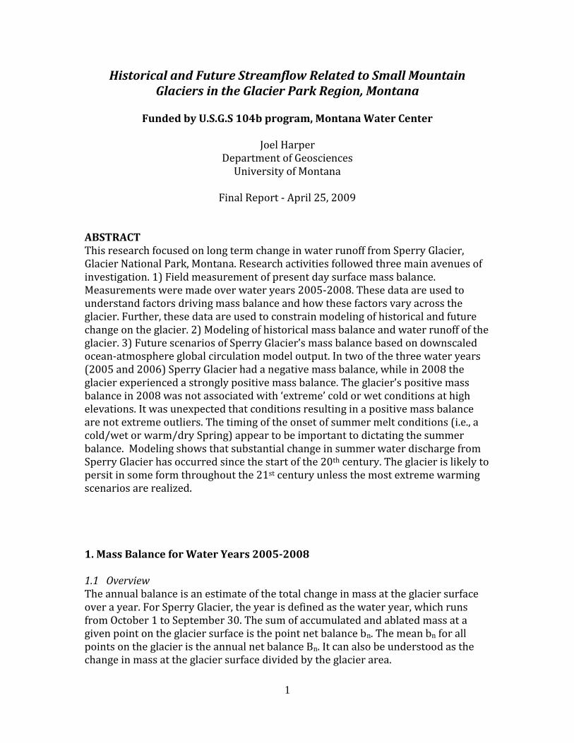
1
Historical and Future Streamflow Related to Small Mountain Glaciers in the Glacier Park Region, Montana
Funded by U.S.G.S 104b program, Montana Water Center
Joel Harper
Department of Geosciences University of Montana
Final Report - April 25, 2009
ABSTRACT This research focused on long term change in water runoff from Sperry Glacier, Glacier National Park, Montana. Research activities followed three main avenues of investigation. 1) Field measurement of present day surface mass balance. Measurements were made over water years 2005-2008. These data are used to understand factors driving mass balance and how these factors vary across the glacier. Further, these data are used to constrain modeling of historical and future change on the glacier. 2) Modeling of historical mass balance and water runoff of the glacier. 3) Future scenarios of Sperry Glacier’s mass balance based on downscaled ocean-atmosphere global circulation model output. In two of the three water years (2005 and 2006) Sperry Glacier had a negative mass balance, while in 2008 the glacier experienced a strongly positive mass balance. The glacier’s positive mass balance in 2008 was not associated with ‘extreme’ cold or wet conditions at high elevations. It was unexpected that conditions resulting in a positive mass balance are not extreme outliers. The timing of the onset of summer melt conditions (i.e., a cold/wet or warm/dry Spring) appear to be important to dictating the summer balance. Modeling shows that substantial change in summer water discharge from Sperry Glacier has occurred since the start of the 20th century. The glacier is likely to persit in some form throughout the 21st century unless the most extreme warming scenarios are realized. 1. Mass Balance for Water Years 2005-2008 1.1 Overview The annual balance is an estimate of the total change in mass at the glacier surface over a year. For Sperry Glacier, the year is defined as the water year, which runs from October 1 to September 30. The sum of accumulated and ablated mass at a given point on the glacier surface is the point net balance bn. The mean bn for all points on the glacier is the annual net balance Bn. It can also be understood as the change in mass at the glacier surface divided by the glacier area.

2
The point net balance bn can be calculated for any point for which both bw and bs are known by summing the two values. A positive sum represents a net gain in mass at the point, while a negative sum represents a net loss in mass. For Sperry Glacier, a direct calculation of bn is possible for the ablation stake points each year. The interpolated bw and bs values also allow bn to be estimated for each 10 m cell by summing the two grids. The mean value for the cells approximates the annual net balance Bn. This method for determining Bn can be used for 2005 and 2006 because there were sufficient snow depth measurements to interpolate bw across the glacier. For 2007 and 2008, Bn is estimated by adding the scaled Bw and the Bs determined through interpolation. 1.2 Methodology We used two methods for calculating Bn. For 2005 and 2006, grids of interpolated bw and bs were both available, allowing calculations of bn for each of the 10 m cells by summing the two grids. The mean bn value is equivalent to the Bn for the glacier as a whole. For 2007 and 2008, only one of the two grids was available, the grid of interpolated bs values. We calculated Bn by summing the Bw value for each year derived via scaling and the Bs value for each year taken from the interpolated grid of bs values. 1.3 Results for 2005 and 2006 water years Maps of interpolated bn for 2005 and 2006 show similar spatial patterns. In both years, the area with the most negative bn values was near the west margin of the glacier, in the area of crevasses and shallow snow. The areas with the highest values were below the headwall and the cirque walls, while the headwall itself showed both positive and negative mass balances. In both years, most of the lower part of the glacier had bn values between -1.00 to -2.00 m w.e. However, while the line where accumulation and ablation are equal – the zero contour – was at different elevations in the two years. In the basin below the headwall, the line was between 2500 and 2550 m elevation both years but in 2006 the line was lower and extended northeast under the cirque wall whereas in 2005 there were only a few patches of positive mass balance under the cirque wall. The maps also showed that the two years had very different accumulation- area ratio (AAR). This measure is the ratio of the area in which the bn is positive to the area of the entire glacier surface. For the glacier area in the denominator of this ratio we used the total area of the interpolated cells – 0.828 km2 - which is slightly smaller than the actual area of the glacier - 0.841 km2. The AAR for 2005 was 0.08, only 1/3 the of 2006 value of 0.24. Both values are well below the ratio of 0.6-0.7 considered typical of a glacier with a positive mass balance.
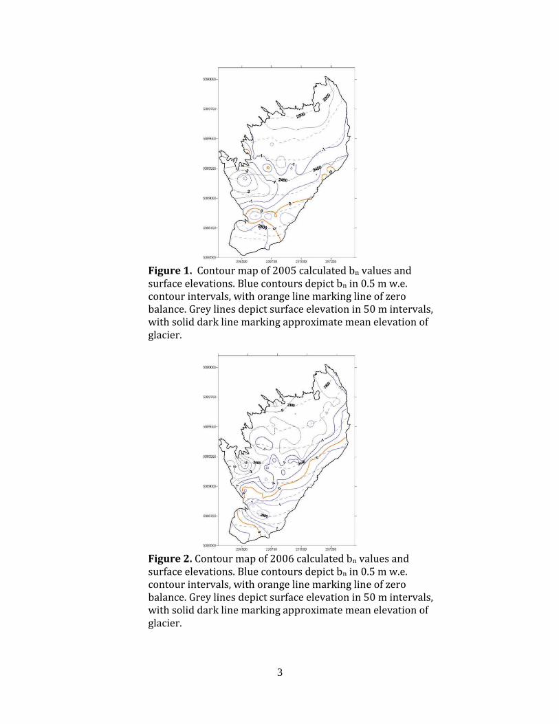
3
Figure 1. Contour map of 2005 calculated bn values and surface elevations. Blue contours depict bn in 0.5 m w.e. contour intervals, with orange line marking line of zero balance. Grey lines depict surface elevation in 50 m intervals, with solid dark line marking approximate mean elevation of glacier.
Figure 2. Contour map of 2006 calculated bn values and surface elevations. Blue contours depict bn in 0.5 m w.e. contour intervals, with orange line marking line of zero balance. Grey lines depict surface elevation in 50 m intervals, with solid dark line marking approximate mean elevation of glacier.

4
The differences between the 2005 and 2006 interpolated bn values were greatest at the extremes. The median values for the two years were nearly identical, as were the 75th-percentile values, with the 25th percentile values similar. Thus the middle 50% of the values were both similar and similarly distributed. For the other two quartiles, particularly the uppermost quartile, the two year’s values were more different. In 2005, the mean and median values were with 0.05 m w.e.; in 2006, the mean was considerably further from the median and closer to the 75th percentile. In 2005, the glacier lost 8.88 x 10⁵ m3 water while gaining just 2.3 x 10⁴ m3, for a net volume change of -8.65 x 10⁵ m3 of water. Dividing that net change by the gridded area results in an annual net balance Bn for the year of -1.04 m w.e. That figure is slightly lower than the mean interpolated bn due to the equation used to determine volume on the grid; the latter is likely a slightly better estimate of bn because the math is simpler. The volume of water lost at the glacier surface in 2006 was 8.53 x 10⁵ m3, only slightly lower than in 2005. The volume gained, however, was 1.54 x 10⁵ m3, 6.5 times greater than in the prior year. The resulting net change for the year was -6.99 x 10⁵ m3 of water, for an annual net balance of -0.84 m w.e. The mean bn of -0.81 was slightly more positive and is again a slightly better estimate of Bn. 1.4 Results 2007 and 2008 water years For these two years, computing the Bn required subtracting the interpolated Bs from the Bw value derived by scaling. However, the ablation stake data provided measured bw values that could be included in the scaling, so the Bw estimate was revised (Table 1). The revised Bw values were each 0.04 m w.e. greater than the previous versions, but the increases seem reasonable. The 2005 value is still within 3% of the interpolated value, and the mean measured bw for 2007 and 2008 are almost certainly underestimate the actual values.
Table 1 2007 2008
Scaled Bw 2.35 3.08
Interpolated Bs -3.97 -2.36
Bw-Bs -1.62 0.72
Mean stake bw 2.44 3.18
Mean stake bs -3.97 -2.4
Mean stake bn -1.53 0.78 Total Grid Area (m2) 808900 808900 Net delta Volume (m3)
-1309090 584952
Without interpolating values we cannot compare spatial patterns with previous years, but other comparisons are possible. Multiplying the total grid area for the Bs

5
computations – slightly smaller than the grid used for the previous two years – by the Bn provides an estimate of net volume change for the glacier in each of the two years. In 2007, the glacier lost a net volume of 1.31 x 10⁶ m3 of water – 86% more than the previous year. In contrast, the glacier gained 5.85 x 10⁵ m3 of water. 1.5 Cumulative Balance: Over the four years of study, an average of 10.4 m w.e. accumulated at any given point on the glacier surface, but 13.11 m w.e. was ablated over the same period (Table 2). The cumulative mass balance for the four years was -2.77 m w.e., with a mean annual balance of -0.69 m w.e. The average volume change each year was -5.72 x 10⁵ m3 of water, for a net volume change over the period was -2.29 x 10⁶ m3. Table 2.
2005 2006 2007 2008 Cumulativ
e Sum Annual Mean Range
Bw (m w.e.)
2.18 2.79 2.35 3.08 10.4 2.60 0.9
Bs (m w.e.)
-3.18 -3.60 -3.97 -2.36 -13.11 -3.28 1.61
Bn(m w.e.)
-1.06 -0.81 -1.62 0.72 -2.77 -0.69 2.34
Net D Volume (m3)
-86481
9
-698469
-130909
0
584952
-2287426 -
571857
1894042
2. Historical Change in Sperry Glacier 2.1. Change in Runoff over the 20th Century
Direct measurements of runoff from Sperry Glacier (or any other GNP glacier)
are not available. We employ two methods to compute present day summer ablation
from the glacier and make the assumption that all ablation results in runoff. First, we
employed a distributed energy balance model, adjusted from Brock and Arnold (2000),
using data from an on-site meteorological station. This modeling supports the notion that
little ablation results from sublimation or evaporation and that shortwave energy is the
dominant source for melting the ice. Second, we made direct measurement of surface
melt using an ablation stake network and continuous measurements of melt at a single
point with a sonic ranger. Ablation measurements showed daily melt rates averaged 56 to
59 mm w.e. during summer and revealed little to no elevation gradient along the glacier.
The distributed energy balance model slightly underestimated the daily melt, and had a
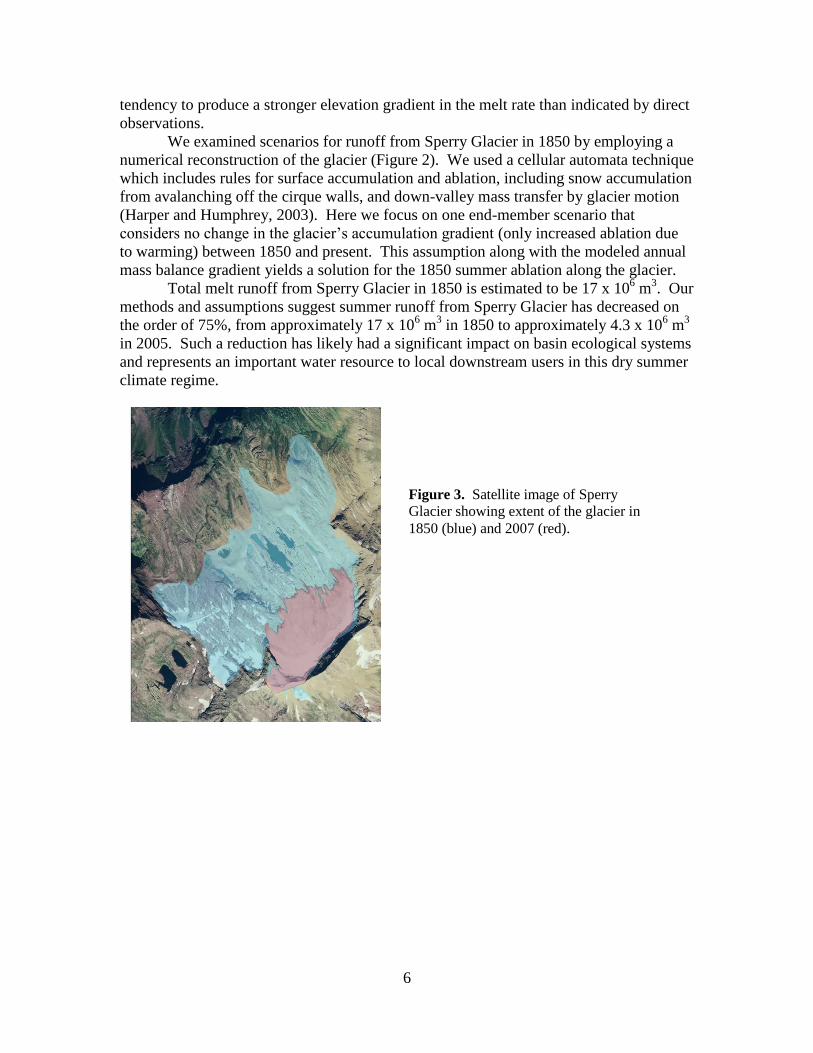
6
tendency to produce a stronger elevation gradient in the melt rate than indicated by direct
observations.
We examined scenarios for runoff from Sperry Glacier in 1850 by employing a
numerical reconstruction of the glacier (Figure 2). We used a cellular automata technique
which includes rules for surface accumulation and ablation, including snow accumulation
from avalanching off the cirque walls, and down-valley mass transfer by glacier motion
(Harper and Humphrey, 2003). Here we focus on one end-member scenario that
considers no change in the glacier’s accumulation gradient (only increased ablation due
to warming) between 1850 and present. This assumption along with the modeled annual
mass balance gradient yields a solution for the 1850 summer ablation along the glacier.
Total melt runoff from Sperry Glacier in 1850 is estimated to be 17 x 106 m
3. Our
methods and assumptions suggest summer runoff from Sperry Glacier has decreased on
the order of 75%, from approximately 17 x 106 m
3 in 1850 to approximately 4.3 x 10
6 m
3
in 2005. Such a reduction has likely had a significant impact on basin ecological systems
and represents an important water resource to local downstream users in this dry summer
climate regime.
Figure 3. Satellite image of Sperry
Glacier showing extent of the glacier in
1850 (blue) and 2007 (red).

7
2.2. Ice Volume Changes 1950-2007 Digital elevation models of Sperry Glacier were constructed from two USGS topographic maps based on surveys of the glacier conducted in 1950 and 1960. A third digital elevation model was produced from data collected during a 2007 survey of the glacier’s surface and surrounding rock margin. This latter survey was done with a kinematic GPS survey system utilizing an established local base station and a rover outfitted with Trimble R7 receivers. Post processing of these data allowed for cm-scale vertical and horizontal accuracy. Digital elevation models were gridded into 10m2 cells via a standard Kriging algorithm. The grids were differenced in order to calculate volume changes between the survey years.
These results provide insight into the rate of ice volume loss of glaciers in Glacier National Park, and constitute figures from which mass balance values could be derived and then compared to current on-going field measurements. The implications of this research are highly relevant at both local and global scales. Locally, up to 75% of water resources in the Rocky Mountain West come from mountain snow, with glaciers filling an important niche as storage reservoirs that provide water during the late summer drought typical for the region. Global scale implications include insight into the fate of runoff from small mountain glaciers. These glaciers are the dominant contributor to current worldwide sea level rise, though the functions by which this is occurring are not yet fully understood.
Figure 4. Modeled geometry and mass balance of Sperry Glacier. Left
panel shows 2007 extent of the glacier. Colors indicate surface mass
balance from a spatially distributed energy balance model. Hotter colors
indicate more negative mass balance. Right panel shows 1850 geometry of
the glacier from a cellular automata model and a spatially prescribed net
mass balance.
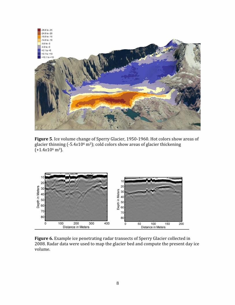
8
Figure 5. Ice volume change of Sperry Glacier, 1950-1960. Hot colors show areas of glacier thinning (-5.4x10⁶ m3); cold colors show areas of glacier thickening (+1.4x10⁶ m3).
Figure 6. Example ice penetrating radar transects of Sperry Glacier collected in 2008. Radar data were used to map the glacier bed and compute the present day ice volume.
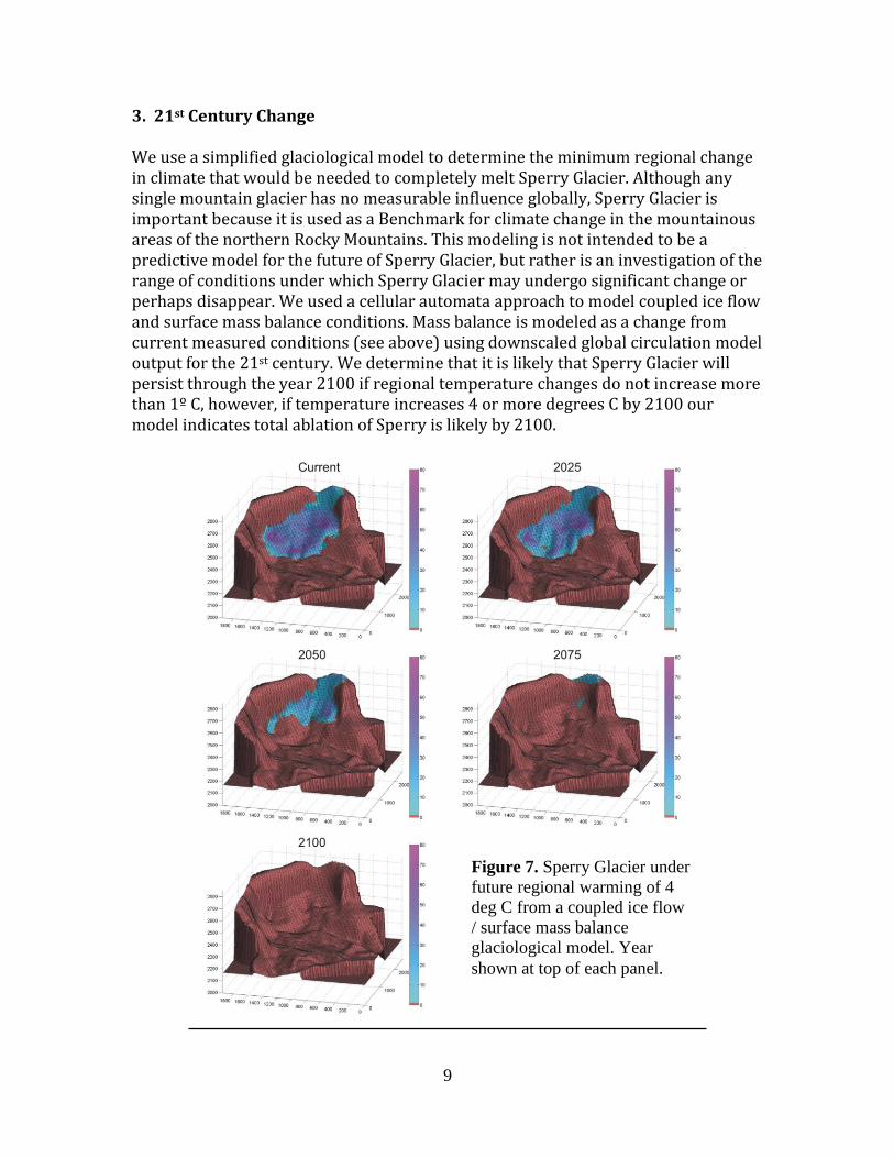
9
3. 21st Century Change We use a simplified glaciological model to determine the minimum regional change in climate that would be needed to completely melt Sperry Glacier. Although any single mountain glacier has no measurable influence globally, Sperry Glacier is important because it is used as a Benchmark for climate change in the mountainous areas of the northern Rocky Mountains. This modeling is not intended to be a predictive model for the future of Sperry Glacier, but rather is an investigation of the range of conditions under which Sperry Glacier may undergo significant change or perhaps disappear. We used a cellular automata approach to model coupled ice flow and surface mass balance conditions. Mass balance is modeled as a change from current measured conditions (see above) using downscaled global circulation model output for the 21st century. We determine that it is likely that Sperry Glacier will persist through the year 2100 if regional temperature changes do not increase more than 1º C, however, if temperature increases 4 or more degrees C by 2100 our model indicates total ablation of Sperry is likely by 2100.
Figure 7. Sperry Glacier under
future regional warming of 4
deg C from a coupled ice flow
/ surface mass balance
glaciological model. Year
shown at top of each panel.

10
Students Involved In (And Supported By) This Research Joel Brown, Ph.D. candidate, Geophysics Michiel Kramer, Ph.D. candidate, Geosciences Blase Reardon, M.S. candidate, Geosciences Nathan Taylor, undergraduate senior, Geosciences James St. Clair, undergraduate senior, Geosciences and Physics Public Outreach Involving This research • Presentation. “Role of Ice Movement in the Response of Glacier Park Glaciers to Climate Change” Waterton-Glacier Parks Science and History Day, July 27, 2006. • Invited guest speaker, Big Sky Science Partnership Summer Institute, June 19, 2008 - Presented an afternoon session on Climate Change and Climate Science Research to ~45 middle school teachers. • Keynote Address (1 hr banquet address) “Glacier Melt and Sea Level Rise: Myths, Realities and Wildcards”, NOAA Great Divide Weather Workshop, Great Falls, MT. October 4, 2007. • Invited Presentation, Glacier-Waterton Peace Park Science Symposium “From
Glacier Park to Greenland: Why Small Glaciers Matter to Sea Level Rise”. July 22, 2008.
Undergradute Senior Thesis Nathan Taylor, UM Geosciences. “Ice Volume Changes in Sperry Glacier, Glacier National Park, From 1950-2007” Completed: 5/2008 Conference Presentations and Publications Kramer, M., and J. T. Harper (2007), Historical Changes in Streamflow Related to
Small Mountain Glaciers in the Glacier Park Region, Montana, U.S.A., paper presented at Workshop on Glaciers in Watershed and Global Hydrology, International Commission for Snow and Ice Hydrology, IAHS, Obergurgl, Austria.
Reardon, B. A., J. T. Harper, and D. B. Fagre (2008), Mass Balance Sensitivity Of
Cirque Glaciers In The Northern U.S. Rocky Mountains, Montana, U.S.A, in Workshop on mass balance measurements and modeling, edited by J. O. Hagen, et al., pp. 1-5, International Glaciological Society, Skeikampen, Norway.
11
Reardon, B.A., J.T. Harper, and D.B. Fagre, 2008, Climatic And Topographic Influences On The Mass Balance Of A Receding Cirque Glacier, Glacier National Park, Montana, Mountain Climate Research Conference, Silverton Colorado, Consortium for Integrated Climate Research in Western Mountains.
Moore, J. N., J. T. Harper, W. W. Woessner, and S. Running (2007), Headwaters of the
Missouri and Columbia Rivers WATERS Test Bed site: Linking Time and Space of Snow Melt Runoff in the Crown of the Continent, Eos Trans. AGU, 88(52), Fall Meet. Suppl., Abstract H13A-0964.

Predictive Modeling of Snowmelt Dynamics: Thresholdsand the Hydrologic Regime of the Tenderfoot CreekExperimental Forest, Montana
Basic Information
Title: Predictive Modeling of Snowmelt Dynamics: Thresholds and the Hydrologic Regimeof the Tenderfoot Creek Experimental Forest, Montana
Project Number: 2007MT150BStart Date: 3/1/2007End Date: 2/28/2009
Funding Source: 104BCongressional
District: At Large
Research Category: Climate and Hydrologic ProcessesFocus Category: Hydrology, Climatological Processes, Models
Descriptors:Principal
Investigators: Lucy Marshall, Brian Leonard McGlynn, Tyler Smith
Publication
Jencso, K. J., B. L. McGlynn, M. N. Gooseff, S. M. Wondzell, and K. E. Bencala. 2009. HydrologicConnectivity Between Landscapes and Streams: Transferring Reach and Plot Scale Understanding tothe Catchment Scale, Water Resources Research. doi:10.1029/2008WR007225.
1.
Smith, T. J., and L. A. Marshall (2008), Bayesian methods in hydrologic modeling: A study of recentadvancements in Markov chain Monte Carlo techniques, Water Resources Research, 44, W00B05,doi:10.1029/2007WR006705.
2.
Smith, T. J., and L. A. Marshall (2009), Exploring uncertainty and model predictive performanceconcepts via a modular snowmelt-runoff modeling framework, Environmental Modelling & Software,Under Review
3.
Smith, T. J. 2008. A Conceptual Precipitation-Runoff Modeling Suite: Model Selection, Calibrationand Predictive Uncertainty Assessment. M.S. thesis, Montana State Univ., Bozeman, MT.
4.
Smith, T. J., and L. A. Marshall. 2008. Development and Application of a ParsimoniousSnow-Hydrologic Modeling Suite: Investigating the Link Between Model Complexity and PredictiveUncertainty. Eos Trans. AGU, 89(53), Fall Meet. Suppl. AGU Fall Meeting 2008. December 15-19.San Francisco, California.
5.
Jencso, K. J., B. L. McGlynn, M. N. Gooseff, S. M. Wondzell, and K. E. Bencala. 2009. HydrologicConnectivity Between Landscapes and Streams: Transferring Reach and Plot Scale Understanding tothe Catchment Scale, Water Resources Research. doi:10.1029/2008WR007225.
6.
Predictive Modeling of Snowmelt Dynamics: Thresholds and the Hydrologic Regime of the Tenderfoot Creek Experimental Forest, Montana
Predictive Modeling of Snowmelt Dynamics: Thresholds and the Hydrologic Regime of the Tenderfoot Creek Experimental Forest, Montana1

Final Report for USGS 104b Grant: Predictive Modeling of Snowmelt
Dynamics: Thresholds and the Hydrologic Regime of the Tenderfoot
Creek Experimental Forest, Montana
Principal Investigators:
Lucy Marshall, Assistant Professor of Watershed Analysis, Department of Land Resources and
Environmental Sciences, Montana State University.
Brian McGlynn, Associate Professor of Watershed Hydrology, Department of Land Resources and
Environmental Sciences, Montana State University.
Abstract This project was aimed at advancing understanding of the first-order controls on snowmelt runoff
processes for improved forecasting and water resource management. The need for this improved insight
is particularly relevant given our reliance in the inland northwest region on mountain water resources,
and our relatively poor understanding of thresholds and controls on runoff generation in mountain
environments. We addressed these themes via a synthesis of field observations, data analyses and
conceptual model development. We undertook our activities at a regional test watershed, the
Tenderfoot Creek Experimental forest, located in the Little Belt Mountains in central Montana.
Our field observations and modeling approaches provided insight to the variables controlling runoff
source areas and the utility of different data for quantifying these. Our analyses indicated topographic
controls on runoff and the variability of this through time. We implemented a modular suite of 30 model
structures to assess the relative importance of different elements of watershed runoff. Our results
emphasize the importance of characterizing the spatial distribution of snowmelt (strongly correlated to
aspect and elevation), and its temporal variability according to climatic indicators such as temperature
and radiation. These results are transferable to other catchments and will help guide future conceptual
models of watershed behavior in mountainous regions.
A self‐contained graphical user interface was developed to integrate the modeling framework and
associated analyses into a freely available modeling software package. The Simulation and Prediction
Lab for Analysis of Snowmelt Hydrology (SPLASH) has been successfully programmed to perform model
selection, parameter calibration, uncertainty analysis, and model evaluation.
This project provided training for two graduate students in field hydrology methods and modeling.
These students were highly productive and successful over the duration of the project. Additionally,
three journal manuscripts and numerous presentations disseminated the main scientific findings of this
project to the greater scientific community.
Introduction and Overview In mountainous areas across the western United States including Montana, winter snowpack controls
regional water resources, supplying water to downstream, lower elevation valleys partially because of

reduced evaporation, greater water deposition, and storage until spring snowmelt. To date, little
research has been conducted in the Montana region on the linkages between snow accumulation, melt
timing, topographic structure, runoff source areas, and streamflow residence time. Although there is a
strong desire to more efficiently predict and model snowmelt driven streamflow yield and timing, the
primary controls on watershed runoff and flow dynamics are poorly understood.
Forecasting watershed response to incident and accumulated precipitation is more easily achieved via
the use of simulation modeling. Such hydrological models play an important role in testing our
understanding of the watershed response to precipitation, whether it is to elucidate more information
on the unobservable processes occurring or to simulate past or future scenarios for better water
resource management. In recent years, hydrologic
modelers have increasingly recognized the
importance of incorporating uncertainty in the
modeling process. Modeling by its nature is only an
approximation of the processes occurring and
significant uncertainties arise in mathematically
expressing complex non-linear watershed
dynamics.
This project aimed to improve understanding and
quantitative modeling of snow accumulation and
melt, watershed streamflow generation, and the
effect of watershed topographic structure on
watershed processes. We focused our efforts on
continued data collection, isotopic analyses of
streamflow residence times, and conceptual model
comparisons.
Research was conducted at Tenderfoot Creek
Experimental Forest (TCEF). The TCEF was
established in 1961, and consists of seven gauged
watersheds (Figure 1). The forest is representative
of the vast expanses of lodgepole pine found east
of the continental divide and is the only USDA
experimental forest formally dedicated to research on subalpine forests on the east slope of the
northern Rocky Mountains.
Objectives 1. To synthesize extensive existing field observations at the Tenderfoot Creek Experimental Forest
into a conceptual predictive modeling framework evaluating the first order controls on spatio-
temporal runoff dynamics, new snowmelt/old groundwater runoff partitioning and the impact
of terrain and forest practices.
Figure 1. Site location and instrumentation of the
TCEF catchment. (a) Catchment location in the Rocky
Mountains, MT. (b) Catchment flumes, well transects,
and SNOTEL instrumentation locations. Transect
extents are not drawn to scale.

2. To initiate watershed tracer experiments quantifying new snowmelt runoff direct contributions
to streamflow and resident (old) groundwater contributions to spring runoff across sub-
watersheds to explicate the residence time of new water within in each of 7 watersheds and
better inform conceptual model underpinnings.
Methodology This project focused on three main activities: hydrometric and isotopic data collection, analysis of
detailed field measurements to inform conceptual modeling, and implementation of a modular
predictive modeling framework.
Hydrologic Data Collection
This project helped support existing infrastructure and allowed for new data collection at the project test watershed. Under this project, continuing data collection included:
Stream flow Monitored discharge at the outlets of 7 nested watersheds Monitored real time specific conductance and temperature at 8 locations
Wells and piezometers Installed (many existing) and monitored (real‐time water level data collection)
100 wells 20 piezometers
Lysimeters Installed recording snowmelt lysimeters
Rainfall Built and installed an incremental rainfall sampler Monitored 5 existing recording rain gauges
We additionally collected water samples for isotopic, dissolved organic carbon (DOC), and major ion
analysis from stream flumes, groundwater wells, piezometers, snow and soil lysimeters, and rainfall
sampler.
Data Analyses
Since the project inception (and following reviewer comments), the project evolved to consider
topographic and water table data (additional to isotopic analyses) to help inform conceptual model
underpinnings and to address major project objectives. In steep headwater catchments with shallow
soils, topographic convergence and divergence is a hypothesized first‐order control on the distribution
of soil water and groundwater. Additionally, hillslope‐riparian water table connectivity represents the
linkage between the dominant catchment landscape elements (hillslopes and riparian zones) and the
channel network. To explore these concepts, we combined digital elevation model (DEM) based terrain
analyses with high frequency water table measurements. Using these, we tested the relationship
between watershed topography and hillslope-riparian‐ stream shallow groundwater connectivity.

We quantified water table connectivity (Figure 2) based on 146 recording wells and piezometers
distributed
across transects
within
Tenderfoot
Creek.
Correlations
were observed
between the
longevity of
water table
connectivity
and the size of
each transect’s
upslope
accumulated
area (Jencso et
al., 2009). We
applied this relationship to the entire stream network to quantify landscape scale connectivity through
time and determine its relationship to catchment scale runoff dynamics. We found that the shape of the
estimated annual landscape connectivity duration curve was highly related to the catchment flow
duration curve (Figure 2). This research suggests internal catchment landscape structure (topography
and topology) as a 1st order control on
runoff source area and whole
catchment response characteristics.
We made additional analyses of isotopic
data to discretize new (snowmelt
runoff) and old (groundwater)
contributions to streamflow. The model
we implemented computes transfer
functions for event water and pre-event
water calculated from a time-variable
event water fraction (Weiler et al.,
2003). This undertaking helped to
identify several obstacles in using
traditional residence time analyses for a
watershed system such as TCEF. The
biggest stumbling block to these
analyses is adequately characterizing the
snowmelt contribution to runoff, due to the strong spatial variability of snow melt patterns across the
watershed. Figure 3 illustrates the inability of classical transfer function models to capture patterns of
Figure 2. A) Upland-stream water table connectivity as a function of upslope accumulated
area. This relationship defines the fraction of the stream network hydrologically
connected to uplands and can be used either as a spatially explicit variable or as a space-
time distribution. B) Flow duration curve and fractional upland stream connectivity curves
for one TCEF subwatershed. Note relationship between connectivity and discharge.
Figure 3. Observed and predicted streamflow from runoff
component of residence time model

runoff. These findings helped support conceptual model methodologies (detailed following). Our project
evolved to focus on characterizing the variability in snow melt rates due to elevation and aspect across
the watershed.
Modeling
We developed and implemented a modular modeling framework that applies model parameter
estimation and uncertainty analysis quantification for a range of hydrologic models. We applied the
modeling framework using existing observations from the Stringer Creek watershed, located within
TCEF. Thirty unique modular structures, ranging in complexity from very simple to moderately complex,
were developed and included in the modeling suite. The suite of models was constructed in a modular,
component‐wise fashion to allow for different conceptualizations of soil moisture accounting, runoff
routing, and snowmelt accounting. We used findings from our data analyses to help guide conceptual
modeling development, focusing on characterizing spatial variability in snowmelt rates, and spatial
variability in runoff source areas.
In implementing the modeling approach we compared three recently developed Markov chain Monte
Carlo algorithms necessary to for model calibration (parameter estimation) and uncertainty analysis
under a Bayesian inferential approach (Smith and Marshall, 2008). The predictive modeling framework
was used to assess the effect of model structural complexity on model predictive performance (Figure
4). We assessed each of the models based on their predictive performance, the uncertainty associated
with the model simulations and parameters, and their ability to predict snow water equivalents (Smith
and Marshall, 2009).
A self‐contained graphical user interface was developed to integrate the modeling framework and
associated analyses into a freely available modeling software package. The Simulation and Prediction
Lab for Analysis of Snowmelt Hydrology (SPLASH) has been successfully programmed to perform model
selection, parameter calibration, uncertainty analysis, and model evaluation. This software package
simplifies the complexities required to implement a predictive modeling study and shifts the focus
toward the modeling problem itself through the application of forward‐looking methods in
computational hydrology.

Figure 4. Modeling framework structural uncertainty and streamflow simulation for 'optimal' modular
structure. Inset shows three model simulations corresponding to different conceptualizations of snowmelt.
Results and Conclusions Overall, the project was successful and productive from three main viewpoints: scientific merit and
furthering scientific understanding, graduate student training, and disseminating results via publications
and presentations. These areas are detailed following.
Scientific Merit
Our analyses of water table connectivity strongly indicates topography (as represented by upslope
accumulated area) controls upland-stream connectivity and that this drives runoff generation through
time. The transformative nature of this research is strongly evident. How hillslope inputs along stream
networks are linked to catchment-scale response has traditionally been poorly understood, with
research efforts focused on a specific plot/stream reach. This project provides implications for
watershed drivers that may be transferable to other catchments and allows development of general
principles that can guide future conceptualizations of watershed models.
In undertaking conceptual model development at our test site, we focused on model selection,
calibration, uncertainty analysis, and overall assessment. The results of this case study suggest that a
modular framework is useful in identifying the interactions between and among different process
representations and their resultant predictions of stream discharge. Such an approach can strengthen
model building and address an oft ignored aspect of predictive uncertainty; namely, model structural

uncertainty. Our modeling approach offers insight into the interplay among the modular components
and predictive performance for TCEF. The overriding conclusions are (1) precipitation semi-distribution
methods did little more than provide another degree of freedom to the model structures; (2) net
radiation is an important component in conceptualization of snowmelt accounting methods; and (3) a
model based on topographic similarity may inhibit the overall calibration performance due to the
model’s rigidity in structure.
While the research undertaken in this project has been focused at a local test-site, the methods and
models developed are broad reaching and could be applied to other watersheds. This research should
have significant impact for better understanding of the link between model reliability and predictive
uncertainty in streamflow forecasting for mountainous snow driven watersheds, and for conceptualizing
watershed response based on topographic structure.
Student Training
Two high achieving graduate students were trained under this project. Kelsey Jencso is pursuing a PhD
degree in the department of Land Resources and Environmental Sciences under the tutelage of Dr Brian
McGlynn. Kelsey’s work focused on hydrologic data collection and data analyses related to hydrologic
connectivity. Kelsey has been very successful while working on this project, and was twice awarded the
American Geophysical Meeting Outstanding Student Paper award. He recently published a high quality
manuscript describing his work under this project and is continuing work focused at TCEF. Tyler Smith
recently completed a Master’s degree and was advised by Dr Lucy Marshall. Tyler’s work focused on
model development, model uncertainty assessment, and construction of the modular modeling
software suite. Tyler published one paper describing the uncertainty methods used in this project, and
has an additional manuscript under review describing the modeling framework. Tyler was additionally
awarded and American Geophysical Meeting Outstanding Student Paper award. This is a highly
competitive award, and it speaks highly of the quality of students supported under this project that both
students received the award. Tyler is continuing his research efforts, and has recently commenced a PhD
degree at Montana State University.
Publications
Several journal papers and numerous presentations resulted out of this project.
Journal Manuscripts
Jencso, K. J., B. L. McGlynn, M. N. Gooseff, S. M. Wondzell, and K. E. Bencala. 2009. Hydrologic
Connectivity Between Landscapes and Streams: Transferring Reach and Plot Scale Understanding to the
Catchment Scale, Water Resources Research. doi:10.1029/2008WR007225.
Smith, T. J., and L. A. Marshall (2008), Bayesian methods in hydrologic modeling: A study of recent
advancements in Markov chain Monte Carlo techniques, Water Resources Research, 44, W00B05,
doi:10.1029/2007WR006705.
Smith, T. J., and L. A. Marshall (2009), Exploring uncertainty and model predictive performance concepts
via a modular snowmelt-runoff modeling framework, Environmental Modelling & Software, Under
Review
Smith, T. J. 2008. A Conceptual Precipitation-Runoff Modeling Suite: Model Selection, Calibration and
Predictive Uncertainty Assessment. M.S. thesis, Montana State Univ., Bozeman, MT.
Presentations
Jencso, K, B L McGlynn, M N Gooseff, R Payn, S Wondzell. 2008. Landscape Structure as a 1st Order
Control on Whole Catchment Hydrologic and Solute Response Characteristics Across Contrasting Climate
Conditions. Fall AGU.
Jencso, K, B.L. McGlynn, M.N. Gooseff, S.M. Wondzell, K.E. Bencala, and R.A. Payn. 2008. Topographic
controls on hillslope–riparian water table continuity in a set of nested catchments, Northern Rocky
Mountains, Montana. CUAHSI (Consortium of Universities for the Advancement of Hydrologic Sciences)
Biennial Colloqium on Hydrologic Science and Engineering
Jencso, K, B.L. McGlynn, M.N. Gooseff, S.M. Wondzell, K.E. Bencala, and R.A. Payn. 2007. Topographic
controls on hillslope–riparian water table continuity in a set of nested catchments, Northern Rocky
Mountains, Montana. American Geophysical Union Fall Meeting. Fall, 2007.
Marshall, L. A.. 2008. Modeling the Catchment Via Mixtures: an Uncertainty Framework for Dynamic
Hydrologic Systems. Uncertainty Quantification Workshop. April 25-26, 2008. University of Arizona,
Tucson, Arizona.
Marshall, L. A. and T. J. Smith. 2008. A Study of Recently Developed MCMC Techniques for Efficiently
Characterizing the Uncertainty of Hydrologic Models. Eos Trans. AGU, 89(53), Fall Meet. Suppl. AGU Fall
Meeting 2008. December 15-19. San Francisco, California.
Marshall, L. A. 2007. University of New South Wales, Sydney, Australia (Invited Seminar). Water
resources research in Montana. [INVITED]
McGlynn, B.L., K. Jencso, K. Gardner, M. Gooseff, and R. Payn. 2008. Climate variability effects on
landscape hydrologic connectivity, riparian buffering potential, and solute fluxes. American Geophysical
Union Fall Meeting. Fall, 2008. [INVITED]
McGlynn, B.L. 2008. Hydrologic connectivity from hillslope to landscape scales: Implications for runoff
generation and water quality. NSF EPSCoR Water Dynamics Workshop, Burlington, VT, Nov 9-11, 2008.
[INVITED]
McGlynn, B.L., K. Jencso, R. Payn, M. Gooseff, T. Covino, and J. Seibert. 2007. Conceptualizing, testing,
and transferring watershed characteristic-runoff generation relationships. Fall AGU [INVITED]
Smith, T. J., and L. A. Marshall. 2008. A Flexible Modeling Framework For Rainfall And Snowmelt.
Montana Section of the American Water Resources Association 25th Annual Meeting. October 2-3,
2008. Big Sky, Montana
Smith, T. J., and L. A. Marshall. 2008. Development and Application of a Parsimonious Snow-Hydrologic
Modeling Suite: Investigating the Link Between Model Complexity and Predictive Uncertainty. Eos Trans.
AGU, 89(53), Fall Meet. Suppl. AGU Fall Meeting 2008. December 15-19. San Francisco, California.

Smith, T, L. Marshall. Predictive modeling of snowmelt and the hydrologic response: Tenderfoot Creek
Experimental Forest, MT. American Water Resources Association Montana Section 24th Annual
Meeting. October 11-12, 2007. Lewistown, Montana.
Smith, T, L. Marshall. A Bayesian uncertainty framework for conceptual snowmelt and hydrologic
models applied to the Tenderfoot Creek Experimental Forest. Eos Trans. AGU, 88(52), Fall Meeting
Supplement. American Geophysical Union Fall Meeting. 10-14 December 2007. San Francisco, CA.
References Cited Jencso, K. J., B. L. McGlynn, M. N. Gooseff, S. M. Wondzell, and K. E. Bencala. 2009. Hydrologic
Connectivity Between Landscapes and Streams: Transferring Reach and Plot Scale Understanding to the
Catchment Scale, Water Resources Research. doi:10.1029/2008WR007225.
Smith, T. J., and L. A. Marshall (2008), Bayesian methods in hydrologic modeling: A study of recent
advancements in Markov chain Monte Carlo techniques, Water Resources Research, 44, W00B05,
doi:10.1029/2007WR006705.
Smith, T. J., and L. A. Marshall (2009), Exploring uncertainty and model predictive performance concepts
via a modular snowmelt-runoff modeling framework, Environmental Modelling & Software, Under
Review
Weiler, M., B. McGlynn, K. McGuire, and J. McDonnell 2003. How does rainfall become runoff? A
combined tracer and hydrologic transfer function approach, Water Resources Research, 39, 1315-1327.

Sediment and Heavy Metals Source Determination andReduction at a Reclaimed Abandoned Mine Site, Alta Mine,Jefferson County, MT
Basic Information
Title: Sediment and Heavy Metals Source Determination and Reduction at a ReclaimedAbandoned Mine Site, Alta Mine, Jefferson County, MT
Project Number: 2007MT152BStart Date: 3/1/2007End Date: 2/28/2009
Funding Source: 104BCongressional
District: At large
ResearchCategory: Water Quality
Focus Category: Water Quality, Hydrogeochemistry, SedimentsDescriptors:
PrincipalInvestigators: Clayton B. Marlow
Publication
Labbe, Richard 2008 "Sediment and Heavy Metals Source Determination and Reduction at aReclaimed Abandoned Mine Site, Alta Mine, Jefferson County, MT" M.S. Dissertation; Departmentof Land Resources and Environmental Sciences; Montana State University, Bozeman, MT (73 pgs)
1.
Sediment and Heavy Metals Source Determination and Reduction at a Reclaimed Abandoned Mine Site, Alta Mine, Jefferson County, MT
Sediment and Heavy Metals Source Determination and Reduction at a Reclaimed Abandoned Mine Site, Alta Mine, Jefferson County, MT1

SEDIMENT AND HEAVY METALS SOURCE DETERMINATION AND
REDUCTION AT A RECLAIMED ABANDONED MINE SITE
ALTA MINE, JEFFERSON COUNTY, MT
by
Richard James Labbe
Advising Faculty Professor
Dr. Clayton Marlow
ABSTRACT
Abandoned hardrock metal mines can have an antagonistic effect on soil
productivity, vegetation, and water quality. Specifically, abandoned mines that actively
generate acidity in soil are phytotoxic due to low pH and increased bioavailability of
heavy metals. Arsenic concentrations in mine soils are often elevated, but may not be as
mobile as heavy metals at low pH. Acid mine drainage migration from abandoned mines
is problematic because it leads to water quality impairments that limit water use for
certain activities (i.e. stock watering and irrigation). In this work, a previously reclaimed
abandoned lead and silver mine (Alta Mine Jefferson County, MT) was characterized for
its persistent impacts on soil, vegetation, and water quality. A progressive monitoring
effort linked offsite water quality impacts to deep underground mine workings, shallow
ground water, and metalliferous soils found at the Alta mine. Water quality impacts were
of importance because they significantly hindered the attainment of Total Maximum
Daily Load (TMDL) allocations that were established shortly before this study.
Vegetative cover on the previously reclaimed portion of the mine was measured in 16
transects in conjunction with 30 soil pits excavated on the reclaimed site. By regression
and analysis of variance, sparse vegetative cover was significantly (p<0.1) linked to pH
and acid generation potential. To overcome acidic soil conditions, lime and compost
amendments were tested on site. The amendments significantly (p<0.1) neutralized soil
acidity; however, a corresponding increase in vegetative cover was not observed.
Erosion of the bare unstable slopes caused greater than anticipated seed bank loss that
precluded vegetation establishment. It is anticipated that successful establishment of a
dense vegetative cover on the abandoned mine could prevent erosion and water quality
impacts due to sedimentation. Vegetation may also have minor impacts on landscape
sources of arsenic and heavy metals that were identified in the study; but the most
significant source of water quality impairment, deep underground mine workings, will
persist at the Alta mine under any land treatment.

1
INTRODUCTION
The science of land rehabilitation integrates principles of soil physiochemistry,
plant physiology, and water interactions. Rehabilitation implies the return to a previous
condition; thus, scientists must examine soil characteristics, plant growth requirements,
and the hydrologic regime of disturbed lands if they are to return them to their original
state. In application, land rehabilitation is the practice of attenuating earth disturbances
and revegetating them by ameliorative, adaptive, or agricultural treatment (Ye et al. 2000,
Tordoff et al. 2000). Mining, timber harvest, agriculture, road building, and other
construction activities commonly result in land disturbances that require rehabilitation.
Watershed processes are explicitly linked to land use; thus, the same suite of disturbances
that often require land rehabilitation may also lead to impairments in bodies of water.
Poor agricultural practices, such as over-fertilization or cattle feeding operations, may
lead to excess nutrient loads in streams; also, mine waste may be an important non-point
source of stream impairment by heavy metals. Nearly all anthropogenic land uses,
including those previously named, are potential sources of excess sediment. The
interconnectedness between land disturbance and watershed impairment is important for
scientists, land managers, and regulatory agencies to understand if they are to implement
effective land rehabilitation and watershed restoration strategies.
Problem Statement
The specific problems addressed in this research are the factors that limit the
rehabilitation of lands disturbed by historic, acid-producing, hard rock metal mines and
the persistent impact that these mines have on water quality on the watershed scale.
Sulfide mineral oxidation resulting in low pH and increased heavy metal toxicity reduces
soil productivity and plant vigor; however, it is not the only process that limits the
successful rehabilitation of mined lands. Soil texture, drought, erosion, lack of organic
matter (OM), low nutrients, and steep slopes exemplify the universe of limitations on
effective mine rehabilitation. In addition, site specific limitations may occur due to
abandoned mine features (i.e. adits, shafts, dumps), site accessibility, and budget
constraints. When chemical, physical, logistical, and fiscal limitations are not overcome,
land rehabilitation is not effective; thus, the potential exists for water quality impairments
downstream. Impairments such as sediment, heavy metals, arsenic, sulfates, and pH may
limit water use for drinking, swimming, irrigation, fish and other organisms.

2
Water Quality in Mined Watersheds
Acid Mine Drainage Impairments
Acid drainage is a term assigned to solutions produced from sulfide mineral
weathering that are characterized by low pH and often contain high levels of potentially
toxic trace elements (e.g. Cd, Zn, Pb,Cu, As). Mining disturbances are a common source
of exposed sulfide minerals; so acid drainage is frequently referred to as acid mine
drainage (AMD). A copious amount of work has been published regarding the formation
of AMD. Comprehensive manuscripts (OSU 1971, Evangelou 1995) discuss the
production chemistry, kinetics, role of microorganisms, and control of AMD. Pyrite
(FeS2) is the most common acid-producing Fe-sulfide mineral and is found in many
geological environments (OSU 1971). The oxidation of pyrite by O2 and subsequent acid
production is the summation of 3 intermediate reactions: 1) dissolution of FeS2; 2)
oxidation of Fe 2+
to Fe 3+
; and 3) hydrolysis of Fe 3+
. Reactions 1 and 3 produce a total
of 5 moles of H+; while 1 mole of H
+ is consumed in reaction 2, resulting in 4 moles of
acidity produced for every mole of FeS2 reacted. Also, at low pH (below 3.5) ferric iron
(Fe3+
) oxidation of pyrite can accelerate acid production to a rate of 16 moles of acid per
1 mole of pyrite reacted (Jennings and Dollhopf, 1995). Reactions assigned to AMD
production, though they are charge and mass balanced, have no molecular, mechanistic,
or rate reaction meaning because pyrite oxidation involves many other metastable species
(Evangelou 1995).
The products of AMD have a significant impact on water quality that is not
limited to the spatial confines of mine disturbances. Rather, historic metal mine
disturbances produce water quality impairments that persist throughout entire watersheds
(Sullivan et al. 2000, Caruso 2003, Herr et al. 2003, U.S. EPA 2006). Sediment, metal
hydroxides, and toxic trace elements (e.g. As, Cd, Cu, Pb, and Zn) from abandoned mine
sources have been shown to cause impairments in fluvial ecosystems (Henry et al. 1999,
Soucek et al. 2000a, Soucek et al. 2000b, Niyogi et al. 2001, Niyogi et al. 2002).
AMD Characterization
Products of AMD and evidence of their negative ecological impact may extend to
all reaches within a watershed; however, several factors make it difficult to characterize
and/or model AMD systems. Heavy metal and As transformations and pH shifts can
occur rapidly in AMD systems at the confluence of waters not impacted by AMD or by
rapid dilution during snowmelt or rainfall events (Brooks et al. 2001, Sullivan et al. 2001,
MacDonald et al. 2007). Mixing with alkaline or neutral streams causes distinct changes
in the chemical signature of AMD (Broshears 1996). Metal hydroxide precipitation in
mixing zones is important in determining downstream aqueous chemical composition.

3
Heavy metal concentrations decrease in mixing zones due to coprecipitation with metal
hydroxides (Runkel and Kimball 2002, Butler II 2006).
In addition to chemical changes brought on by hydrologic influences, the
character of AMD impacted streams is dependent on biological and physical factors.
Reduced stream flows due to evapotranspiration by riparian vegetation can amplify heavy
metal concentrations, as photoreduction and microbial reduction of Fe(III) to Fe(II) is
increased during periods of low flow (Sullivan and Drever 2001, Butler II 2006).
Concentrations of heavy metals in the water column increase when Fe is reduced, either
microbially or by photoreduction, because of decreased adsorption on Fe-hydroxides
(Sullivan and Drever, 2001).
Abandoned metal mines that produce AMD have the potential to discharge As
and heavy metals from a variety of sources. Heavy metals and As may be transported in
leachate from tailings, waste rock, and contaminated soils or may be discharged from
mine workings such as portals, shafts, and adits. For this reason, site specific factors are
possibly the most important in determining how products of AMD are transported in
streams. Kimball et al. (2002) identified numerous inflows springs, bogs, diffuse
sources, seeps, and adits along a 12 km reach of Cement Creek, Colorado. Depending on
the nature of each source, inflows either attenuated or contributed to the transport of
heavy metals and other products of AMD. Recent monitoring and modeling efforts
concluded that abandoned mine features (point sources) were likely the most significant
sources of AMD products (Runkel and Kimball 2002, Kimball et al. 2002, Caruso 2003,
and Herr et al. 2003).
Sediment from Abandoned Mines
As early as the beginning of the 20th
century, impacts of excess sediment from
mining sources were assessed (Gilbert 1917). Hydraulic gold mining led to the
production of nearly 8 billion m3 of mining debris in the Yuba, Bear, and American river
watersheds, some of which negatively impacted the San Pablo, San Francisco, and Suisun
Bays. The spatial extent of sediment delivery from abandoned hard rock mines is not as
vast as that from large hydraulic mine sources but resulting overbank deposits and silted
stream channels are the same. Soda Butte Creek drains the historic New World gold
mining district near Yellowstone National Park. A tailings impoundment failure in 1950
resulted in exposed over-bank tailings deposits as far as 25 km downstream (Marcus et al.
2001). The source of the sediment was unmistakably linked to the tailings impoundment
failure by sand-sized pyrite grains, strong oxidation, and sparse vegetative cover. The
tailings also filled abandoned channels as deep as 0.7 m.
Bonta (2000) monitored 3 Ohio watersheds for suspended sediment in their
natural condition, during active mining and reclamation, and after final reclamation.
Maximum suspended sediment concentrations were the highest in each watershed during
mining and reclamation activities; while, minimum concentrations were always in the
undisturbed condition. In one watershed, average post reclamation suspended sediment
loads were decreased by 75% of the load in the undisturbed condition. The decrease was

4
attributed to increased vegetative cover and not lack of stream power because average
stream flows had actually increased following reclamation.
Limits on Soil Productivity and Vegetation Establishment
Establishing a vegetative cover on land disturbed by historic hard rock mining is
an effective way to reduce erosion, limit heavy metal and As leachate, and improve water
quality within a watershed (Brown 2005); however, there are many chemical and
physical limitations to vegetation establishment on these sites.
Mine Waste
Tailings deposits and waste rock dumps are common remnants of abandoned
mine disturbances that produce AMD. Tailings are the by-product of the ore milling and
concentrating process; as such, they are generally made of fine-grained material (Tordoff
2000). Residual sulfide ore minerals and metals content is high in historic mine tailings
because of inefficiencies in past separation processes (Alloway 1995). Poor vegetation
establishment on fluvially deposited tailings on the banks of the upper Clark Fork River
and on the historic Keating gold and copper mine tailings in Montana are just 2 of the
countless examples of the phytotoxicity of tailings (RRU-BRI 2004, Neuman et al. 2005).
Further, pyrite oxidation occurring as deep as 1 m within mine tailings heaps may lead to
a decline in vegetative cover where increased sulfur oxidizing bacteria are present and
neutralization potential is depleted (Schippers et al. 2000).
In contrast to tailings deposits, waste rock piles are typically composed of larger
rock fragments that have been removed from their native location but have not been
milled or processed. Waste rock piles also have the potential to produce AMD by sulfide
mineral oxidation (Lefebvre et al. 2001, Sracek et al. 2004). It cannot be assumed that
tailings or waste rock pile removal will result in successful remediation of AMD. As a
result of AMD solution leaching from waste rock, native soils beneath waste rock piles
may be enriched with metals in soluble secondary minerals (Zhixum 1997). Low pH in
mine waste substrates and soils in contact with mine waste is a crucial limiting factor to
vegetation establishment.
Revegetation and Rehabilitation
Rehabilitation is successful when acid-metalliferous substrates (i.e. impacted
soils, tailings, waste rock) cease to inhibit plant growth and are no longer mobile in the
environment. In situ amendment of substrate that reduces toxic trace element
bioavailability and raises soil pH has emerged as a commonly practiced treatment in
abandoned acid-metal mine rehabilitation
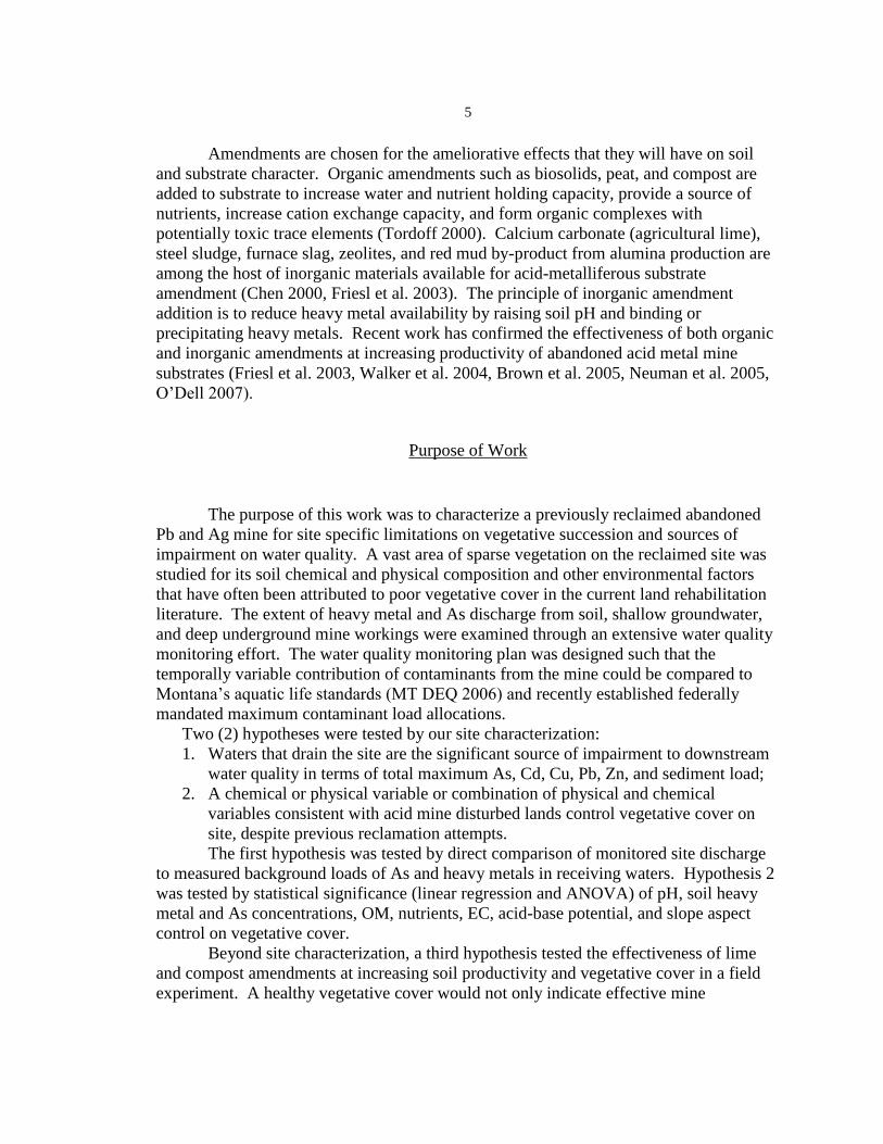
5
Amendments are chosen for the ameliorative effects that they will have on soil
and substrate character. Organic amendments such as biosolids, peat, and compost are
added to substrate to increase water and nutrient holding capacity, provide a source of
nutrients, increase cation exchange capacity, and form organic complexes with
potentially toxic trace elements (Tordoff 2000). Calcium carbonate (agricultural lime),
steel sludge, furnace slag, zeolites, and red mud by-product from alumina production are
among the host of inorganic materials available for acid-metalliferous substrate
amendment (Chen 2000, Friesl et al. 2003). The principle of inorganic amendment
addition is to reduce heavy metal availability by raising soil pH and binding or
precipitating heavy metals. Recent work has confirmed the effectiveness of both organic
and inorganic amendments at increasing productivity of abandoned acid metal mine
substrates (Friesl et al. 2003, Walker et al. 2004, Brown et al. 2005, Neuman et al. 2005,
O’Dell 2007).
Purpose of Work
The purpose of this work was to characterize a previously reclaimed abandoned
Pb and Ag mine for site specific limitations on vegetative succession and sources of
impairment on water quality. A vast area of sparse vegetation on the reclaimed site was
studied for its soil chemical and physical composition and other environmental factors
that have often been attributed to poor vegetative cover in the current land rehabilitation
literature. The extent of heavy metal and As discharge from soil, shallow groundwater,
and deep underground mine workings were examined through an extensive water quality
monitoring effort. The water quality monitoring plan was designed such that the
temporally variable contribution of contaminants from the mine could be compared to
Montana’s aquatic life standards (MT DEQ 2006) and recently established federally
mandated maximum contaminant load allocations.
Two (2) hypotheses were tested by our site characterization:
1. Waters that drain the site are the significant source of impairment to downstream
water quality in terms of total maximum As, Cd, Cu, Pb, Zn, and sediment load;
2. A chemical or physical variable or combination of physical and chemical
variables consistent with acid mine disturbed lands control vegetative cover on
site, despite previous reclamation attempts.
The first hypothesis was tested by direct comparison of monitored site discharge
to measured background loads of As and heavy metals in receiving waters. Hypothesis 2
was tested by statistical significance (linear regression and ANOVA) of pH, soil heavy
metal and As concentrations, OM, nutrients, EC, acid-base potential, and slope aspect
control on vegetative cover.
Beyond site characterization, a third hypothesis tested the effectiveness of lime
and compost amendments at increasing soil productivity and vegetative cover in a field
experiment. A healthy vegetative cover would not only indicate effective mine
6
rehabilitation but could potentially reduce sediment, heavy metal, and As loads from soils
and shallow groundwater. The third hypothesis was:
3. Lime and compost amendments will increase soil productivity and vegetative
cover on experimental treatment plots on the disturbed site.
This hypothesis was tested by the statistical significance of end of growing season soil
and vegetative cover characteristics compared to end of growing season controls.
The results of this work are important to private, state, and federal stakeholders
who may be responsible for the rehabilitation of similar mines in roughly the same
geographic region. This work also exemplifies the complex link between water quality
impairments and acid mine land disturbances. Watershed planners and conservation
districts may consider the results of this work when assessing the impact of abandoned
mines in watersheds of comparable size and character.
Study Site
Location
The study site, located approximately 30 km south of Helena, MT, consists of the
abandoned Alta Mine complex, a small stream referred to as the Alta tributary, and
Corbin Creek immediately above and below its confluence with the Alta tributary (Figure
2). The abandoned Alta mine complex is included in the Colorado Mining District of
Jefferson County, MT (Pioneer 1994). As an abandoned mine, the Alta is not unique. In
fact, it is one of an estimated 6,000 inactive mining and milling sites across Montana
(Pioneer 1994).
The Alta mine complex is divided into an upper mine site and a lower mine site.
The lower site is located in Section 10, T7N, R4W; and the upper site is distributed
between Sections 9 and 10, T7N, R4W. The Alta tributary drains the Alta mine
diagonally from SW to NE across Section 10, T7N, R4W, until it reaches a confluence
with Corbin Creek in the SW1/4 of SW1/4 Section 2, T7N, R4W. The Alta tributary and
Corbin Creek are found at the southern edge of the Lake Helena Watershed in the Upper
Missouri River Drainage Basin. Corbin Creek drains an estimated 442 ha above its
confluence with the Alta tributary. The Alta tributary subwatershed accounts for
approximately 19% (82 ha) of the drainage area. The streams drain to Prickly Pear
Creek, which is the largest stream in the Lake Helena Watershed.
7
Figure 1. Alta Mine Site Location. Points on Montana inlay represent abandoned mines.
Geology and Climate
The elevation of the study site ranges from approximately 1,500 m above mean
sea level (amsl) at the confluence of the Alta tributary and Corbin Creek to 1,905 m-amsl
at the summit of Alta Mountain. Snow in the winter, rain in the spring, and intermittent
thundershowers throughout summer and fall account for precipitation at the site. Snow in
the Alta drainage accumulates primarily on the slopes with northern aspect; while, snow
on the south facing slope tends to melt or sublimate rapidly. The 30-year average
cumulative annual precipitation at the nearest weather station in Boulder, MT is 28.7 cm.
Cumulative precipitation for the latest complete year of record (2006) was 29.3 cm. Both
Deckler (1982) and Tetra Tech (1997) suggested increased precipitation at the Alta Mine
due to orographic effects; and observations made in the summer of 2007 seem to
corroborate this assumption. Cumulative precipitation at the Alta Mine—approximately
190 m above the Boulder weather station—was nearly 6% greater than that observed in
Boulder. Site temperature varies from extreme cold in winter to extreme heat in summer.
Average Monthly temperatures (from Boulder weather station) range from -12 oC to 0
oC
in January and from 7 oC to 26
oC in July (Tetra Tech 1997).

8
The study site is at the north end of the Boulder Batholith and Elkhorn Mountain
volcanics formations. Both formations are igneous and Cretaceous in age; however, the
Batholith is intrusive, while the Elkhorn Mountain volcanics are remnant of lava flows
and volcanic ejecta (Veseth and Montagne 1980). Rocks present on site are
representative of both formations. Quartz monzonite is the primary batholithic rock;
while, rhyolite and dacite tuffs and lava flows account for much of the volcanics (Veseth
and Montagne 1980, Tetra Tech 1997).
Mining History
The Alta mine was the most productive underground lead and silver mine in the
area, owing to an extensive ore body of galena (presumably argentiferous galena), pyrite,
tetrahedrite, and sphalerite (Becraft et al. 1963). Ore was discovered there in 1869; and
the mine operated at its greatest capacity from 1883 to 1896. Minimal amounts of silver
and lead ore were produced after 1896; however, low grade ore, used as silica flux in the
East Helena smelter, was mined in the 1950s. When mining ceased, the site was
abandoned as a pile of waste rock, 13 levels of underground mine workings, and a series
of shafts and adits that opened to the surface on the east side of Alta Mountain. Most
notably, the #8 shaft was a continuous source of metals laden AMD that discharged from
beneath the lower waste rock pile. The waste rock piles consisted of ore minerals
sparsely and heterogeneously distributed within volcanic and batholithic rock materials.
In addition to sulfide minerals from within the Alta ore body, limonite, chalcopyrite, and
quartz were deposited on the lower Alta waste rock dump after exploration in a separate
vein immediately to the southwest. Ore samples from this vein contained 11 % copper.
Samples of crude ore from the Alta ore body were shown to contain 18 – 35 % lead; and
concentrated samples had 12 % zinc.
Reclamation History
Of the estimated 6,000 abandoned mines in Montana, a list of 270 priority
abandoned mine sites was compiled (Pioneer 1994). In 1993, nearly all of the 270 mines
were characterized for their risk to human health and the environment by chemical
degradation and hazardous abandoned structures. Upon characterization, sites were
compared and ranked according to severity of risk. Alta was ranked 17th
amongst the
most threatening mine sites due to metals laden AMD that exceeded nearly all of
Montana’s numeric water quality standards and for its abundance of actively eroding
waste rock dumps with elevated levels of Pb and As (Pioneer 1994).
Reclamation of priority abandoned mine sites is funded largely by the Surface
Mining Control and Reclamation Act (SMCRA) of 1977 and is administered by the
Montana Department of Environmental Quality (MT DEQ 2005). MT DEQ reclaimed
the Alta mine in the summer of 1999. Work done during the reclamation effort included:
removing 117, 741 m3 of waste rock; transporting waste rock to a 2.3 ha repository;

9
reconstructing 274 m of stream channel; re-contouring the 40% slopes with terraces; and
fertilizing, seeding, and mulching the re-contoured area (Tetra Tech 2002). Risk-based
As, Pb, and Mn concentrations were used to determine which portions of the waste rock
to remove. All of the waste rock removal and subsequent reclamation activities were
done exclusively on the lower Alta mine site; while, waste rock piles at the upper mine
and in the Alta tributary below the reclaimed area were left in place. The reclamation
effort did not include surface water or groundwater treatment; however, a failed attempt
to seal the #8 shaft was made in order to eliminate surface discharge (Tetra Tech 2002).
Watershed Restoration
The Clean Water Act (CWA), as amended in 1977, includes programs that aim to
limit the discharge of pollution from industrial point sources, regulate effluent from waste
water treatment plants, and reduce nonpoint source pollution impacts (Gallagher and
Friedman 2001). Section 303(d) of the CWA maintains that each state must assemble a
list of waters that are impaired and the contaminants that impair them. Each state must
assess contaminant sources (point and nonpoint) for a given body of water and determine
the reduction in contaminants needed to support beneficial water uses. The reduced load
is known as a Total Maximum Daily Load (TMDL).
Corbin Creek, the receiving waters of the Alta tributary, has been found to be
impaired by As, Cd, Cu, Pb, Zn, and sediment from its headwaters to its mouth (U.S.
EPA 2006). TMDLs have been established for each of these constituents, along with the
current estimated daily load and the percent reduction required for TMDL attainment
(Table 2). Abandoned mines are estimated to account for 59%, 99%, 96%, 86%, 98%,
and 5% of the As, Cd, Cu, Pb, Zn, and sediment loads in Corbin Creek, respectively. The
remainder of the current load is attributed to dirt roads, timber harvest, natural sources,
and stream bank erosion. Extensive mining and reclamation activities have taken place in
the Corbin Creek watershed above the Alta tributary but not below. Of the many
abandoned metal mines with a potential impact on Corbin Creek, the Alta mine complex
is mentioned by name in the Framework Water Quality Restoration Plan for the Lake
Helena Watershed Planning Area (US EPA 2006); however, the mine’s contribution of
sediment and heavy metals is not directly estimated. Moreover, the document suggests
that the #8 shaft had been sealed during reclamation. While the document recognizes that
limited revegetation of the Alta mine may be a source of sediment and toxic trace
elements, it accounts for less than 0.5 ha of bare ground.

10
Table 1. Corbin Creek TMDL Attainment Goals and Estimated Current Maximum Loads
(US EPA 2006).
Constituent
Estimated Current TMDL
Load (kg day-1
) % Reduction Required (kg day-1
)
Arsenic 0.06 25% 0.045
Cadmium 0.11 97% 0.003
Copper 1.32 89% 0.141
Lead 0.12 66% 0.041
Zinc 72.72 97% 2.045
Siltation 0.59 23% 0.455
Precedent Research
More than a decade before the massive abandoned mine characterization effort
launched by the state of Montana, Deckler (1982) characterized soils and substrates at the
Alta mine. Consistent with the efforts of the state, he found the site to include 2 large
waste piles that were uninhabited by vegetation. The upper Alta waste rock pile was less
acidic (pH from 5.5 to 6.2), coarse textured (and homogenous), and contained lower
concentrations of potentially toxic trace elements than the lower pile. Erosion, nutrient
availability, and overly drained soils were suspected to limit vegetation on the upper pile.
The lower pile was finer textured and more acidic (pH=3.0). Extractable metal levels
were high on the lower waste rock pile but soluble metal levels were low. There was
evidence that metals had leached from upper portions of the waste profile; thus, it is
possible that they reached native soils below. Deckler made several suppositions about
the future reclamation of the site. He concluded that: sufficient cover soil depth must be
maintained on lower slopes to sustain vegetation; upper waste rock material may be used
as a barrier between lower waste rock and cover soil; and mulches would provide
nutrients and decrease incident solar radiation from the bare waste rock piles. Finally,
Deckler (1982) noted that tailings from the nearby Bertha mine were located directly in
the Corbin Creek channel above the Alta tributary at the time of his study. These tailings
were removed in 2002 in a reclamation project separate from the Alta reclamation effort
(MT DEQ 2008).
Schroth (2001) and Schroth and Parnell (2005) provide a thorough account of
geochemical transformations within the Alta waste rock pile prior to its removal and in
the Alta channel following relocation of the pile. They found that schwertmannite
precipitation was an important metal sink within the waste rock pile. It was further
discovered that metal hydroxide precipitation increased upon pile removal; however,
trace element concentrations did not actively decrease by coprecipitation with
schwertmannite. Pre and post waste rock removal concentrations of selected trace
elements in the Alta tributary immediately above Corbin Creek remained relatively
constant (Figure 3).

11
0.01
0.1
1
10
100
1000
Cu Zn Pb Cd As pH
Pre-removal (6/27/99) Post-removal (6/23/00)
Figure 2. Heavy Metal and As Concentrations (mg kg
-1) in Alta Tributary Before and
After Waste Rock Removal. Data are from Schroth (2001).
In effect, Schroth and Parnell (2005) concluded that trace element attenuation by
the waste rock pile was equal to that of attenuation by coprecipitation with Fe-hydroxides
in the channel. All trace elements except for Cu were found to decrease in the direction
of flow in the Alta tributary both before and in the summer after pile removal (Figure 4).
0.01
0.1
1
10
#8 shaft lower Alta above Corbin Corbin below Alta
Cu (pre-removal)
Cu (post-removal)
As (pre-removal)
As (post-removal)
pH (pre-removal)
pH (post-removal)
Figure 3. Cu, As, (mg L
-1) and pH (standard) Along Longitudinal Profile of Alta
Tributary Before and After Waste Rock Removal. Data are from Schroth (2001).
The longitudinal profiles substantiate the idea that pile removal did little to
influence downstream concentrations of heavy metals and arsenic in the first year after
reclamation. Hydrologic regime appears to play an important role in determining
concentrations in Corbin Creek. No surface flow was observed in the creek above the
Alta tributary in 2000. As a result, pH below the Alta tributary was 1 unit less than in

12
1999. Concentrations of Cu and As decreased after mixing with Corbin Creek surface
flows in 1999 but increased or remained constant in 2000—when no flow was observed
in the creek above the confluence with the Alta tributary.
The findings of previous researchers are a time-specific representation of
conditions, processes, and events at the Alta mine. The relevance of each work was
dictated by prevailing site conditions at the time of study. As a means to assess
reclamation alternatives, Deckler (1982) examined the characteristics of two waste rock
piles that had been abandoned for nearly 30 years. Schroth (2001) provided a narrative of
geochemical processes that occurred as a result of transient conditions during the
reclamation effort in the summer of 1999. The current study expands the temporal
coverage of our knowledge about the abandoned Alta mine to include a characterization
of post reclamation site conditions and water quality impacts. The study is relevant
because of an apparent vegetation failure on reclaimed slopes and because of recently
established TMDLs in Corbin Creek.

13
METHODS AND MATERIALS
Soil Survey
Soil Pit Excavation
Post-reclamation soils were surveyed on the Lower Alta reclaimed site in the
summer of 2006. Sharpshooter shovels were used to dig 30 soil pits to completed depths
between 0.6 m and 0.75 m. In most cases, pits were started by scraping surface-exposed
material from the edge of a terrace (Sobek et al. 1978); then, pits were completed by
excavating through topsoil of the adjacent lower terrace to the desired depth. Soil
profiles were described in field notes according to soil color, mottling, moisture, root
zone, and apparent texture. The pits were located on an approximate 25 m grid of the
reclaimed area (Figure 5).
Figure 4. Soil Pit Locations on the Lower Alta Mine Site.
14
To prevent cross contamination between soil pits, they were dug with 2
alternating shovels. Upon completion of a pit, the first shovel was washed and allowed to
air dry while another soil pit was completed with the second shovel. Shovels were
decontaminated with Alconox® detergent dissolved in ambient temperature de-ionized
water at 10 g/L. Decontamination included scrubbing with a wire brush; scrubbing with
a synthetic-bristled brush; and rinsing with de-ionized water for 10 seconds. The
decontamination station was located on the tailgate of our field vehicle. It consisted of a
19 L tub of detergent solution and 15 L of de-ionized rinse water. Shovels were
decontaminated at the end of each sampling day to prevent uncontrolled offsite transfer
of impacted soils.
Soil Sample Collection
Each of the pits was sampled at two intervals: 0 - 15 cm; and 60 - 75 cm.
Sampling at these intervals was completed to remain consistent with the EEECA
sampling protocol (PRC EMI 1997). Between 1 and 1.5 kg of soil was collected from
each interval with multiple scoops of a Corona CT3020 polished aluminum trowel. Soils
were stored and transported in sealed plastic bags, each labeled with soil pit name, date,
and depth interval. As was done with the sharpshooter shovels, trowels were washed
between samples. Four trowels were used for soil sample collection such that two
trowels were in use while the other two were washed. Trowels were carried from the
decontamination station in a separate, clean, dry plastic bag. In addition to soils,
controlled 1.2 mm silica sand was collected with trowels that had been decontaminated at
the time of sampling. The sand, which was transported to the site in a sealed, clean, dry,
plastic bag, underwent all further sample preparation and analysis steps as a blind control.
Like soil samples, it was sampled in 1 to 1.5 kg increments. Trowels were
decontaminated at the end of the day to prevent uncontrolled offsite transfer of impacted
soils.
Soil Sample Preparation
Soil samples were first homogenized by mixing within the sealed plastic bags in
which they were originally collected and transferred; then, they were removed from their
bags and spread onto sheets of brown kraft paper (Sobek et al. 1978) to air dry for at least
24 hours. Each sample was placed on a separate piece of paper and labeled with its soil
pit name, date, and depth interval. While on the kraft paper, each soil sample was mixed
with its own clean spatula in order to accelerate drying and to further homogenize the
samples.
Once samples were dry, they were transferred to clean aluminum pans and
weighed on 10-kg capacity scale. The total weight of each sample was recorded before it
was sieved through a USA Standard No. 10 sieve with 2 mm openings. Each sample was
shaken by hand for approximately 1 minute or until the sample was sufficiently
separated. The samples, less the fraction with particle diameter greater than 2 mm, were

15
returned to their aluminum pans, weighed, and recorded. Only the fraction of each
sample with particle diameter less than 2 mm was retained for soil chemical and textural
analyses. Retained samples were returned to clean, dry, plastic bags and labeled by soil
pit name, depth interval, and date collected. All samples underwent this process as a
minimum of preparation. Additional preparation and methods of specific soil analyses
are outlined below.
Soil Sample Analyses
A multitude of soil physical and chemical properties, known to affect vegetative
succession, were considered in the characterization of the Lower Alta reclaimed site. The
list includes Acid Base Accounting (ABA), heavy metals and arsenic, pH, EC, texture,
rock content, nutrients, and organic matter. Some of the analyses were performed on the
campus of Montana State University; while, others were completed by an independent
laboratory—namely Energy Laboratories Inc. of Billings, MT (Energy Labs).
Rock Content. Rock content of Alta soils was determined as the amount of
material that did not pass through a USA Standard No. 10 (2 mm) sieve (USDA, NRCS
2007). Specifically, rock content of each sample was expressed as a percent of the total
sample by mass.
Soil Texture. Soil texture and class were determined by the hydrometer method
described in Tan (2005) and the USDA Soil Texture Triangle. A mechanical blender was
used to blend 100 g of soil, distilled water (to within 10 cm of the top of a stainless steel
blender cup), and 10 ml of 0.25 M (NaPO3)Na2O (sodium metaphosphate) solution for 15
minutes. The mixture was transferred to a glass ASTM soil testing cylinder; and distilled
water was added until the suspension reached the 1205 ml level. A stirrer was used to
thoroughly mix the suspension; then, a hydrometer was placed in the cylinder.
Hydrometer readings were taken twice at 40 s and again after 2 hrs. The averaged 40 s
readings were taken to be the silt and clay fraction of the soil matrix; and the 2 hr reading
was clay alone. The temperature of the suspension was recorded and used to correct
hydrometer readings to the calibration temperature of 68 oF ( 20
0C).
Paste pH and EC. Saturated pastes (2:1, soil:water) were prepared with soils from
each of the 30 soil pits and sampled depth intervals. The pastes were prepared in 200 ml
paper cups according to Sobek (1978), except that less than 10 mesh soils were used
instead of less than 60 mesh soils. The soils were allowed to wet by capillary action
before being stirred to a thin paste with a spatula. The spatula was rinsed with a jet of de-
ionized water before stirring each sample.
EC was measured with a YSI 3100 Benchtop Conductivity Meter. Before making
EC measurements, the cell constant of the instrument was set at 1.00/cm and it was
calibrated with 8,974 μS and 2,764 μS standard solutions. Additional calibrations were
performed after every 10 soil samples. The YSI 3100 was set to automatically adjust EC
readings with changes in temperature. Measurements were recorded when the digital EC
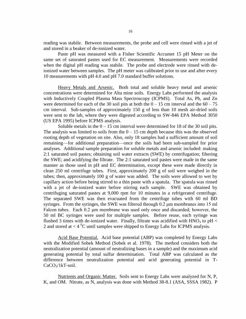
16
reading was stabile. Between measurements, the probe and cell were rinsed with a jet of
and stored in a beaker of de-ionized water.
Paste pH was measured with a Fisher Scientific Accumet 15 pH Meter on the
same set of saturated pastes used for EC measurement. Measurements were recorded
when the digital pH reading was stabile. The probe and electrode were rinsed with de-
ionized water between samples. The pH meter was calibrated prior to use and after every
10 measurements with pH 4.0 and pH 7.0 standard buffer solutions.
Heavy Metals and Arsenic. Both total and soluble heavy metal and arsenic
concentrations were determined for Alta mine soils. Energy Labs performed the analysis
with Inductively Coupled Plasma Mass Spectroscopy (ICPMS). Total As, Pb, and Zn
were determined for each of the 30 soil pits at both the 0 – 15 cm interval and the 60 – 75
cm interval. Sub-samples of approximately 150 g of less than 10 mesh air-dried soils
were sent to the lab, where they were digested according to SW-846 EPA Method 3050
(US EPA 1995) before ICPMS analysis.
Soluble metals in the 0 – 15 cm interval were determined for 18 of the 30 soil pits.
The analysis was limited to soils from the 0 – 15 cm depth because this was the observed
rooting depth of vegetation on site. Also, only 18 samples had a sufficient amount of soil
remaining—for additional preparation—once the soils had been sub-sampled for prior
analyses. Additional sample preparation for soluble metals and arsenic included: making
2:1 saturated soil pastes; obtaining soil water extracts (SWE) by centrifugation; filtering
the SWE; and acidifying the filtrate. The 2:1 saturated soil pastes were made in the same
manner as those used in pH and EC determination, except these were made directly in
clean 250 ml centrifuge tubes. First, approximately 200 g of soil were weighed in the
tubes; then, approximately 100 g of water was added. The soils were allowed to wet by
capillary action before being stirred to a thin paste with a spatula. The spatula was rinsed
with a jet of de-ionized water before stirring each sample. SWE was obtained by
centrifuging saturated pastes at 9,000 rpm for 10 minutes in a refrigerated centrifuge.
The separated SWE was then evacuated from the centrifuge tubes with 60 ml BD
syringes. From the syringes, the SWE was filtered through 0.2 μm membranes into 15 ml
Falcon tubes. Each 0.2 μm membrane was used only once and discarded; however, the
50 ml BC syringes were used for multiple samples. Before reuse, each syringe was
flushed 3 times with de-ionized water. Finally, filtrate was acidified with HNO3 to pH <
2 and stored at < 4 0C until samples were shipped to Energy Labs for ICPMS analysis.
Acid Base Potential. Acid base potential (ABP) was completed by Energy Labs
with the Modified Sobek Method (Sobek et al. 1978). The method considers both the
neutralization potential (amount of neutralizing bases in a sample) and the maximum acid
generating potential by total sulfur determination. Total ABP was calculated as the
difference between neutralization potential and acid generating potential in T-
CaCO3/1kT-soil.
Nutrients and Organic Matter. Soils sent to Energy Labs were analyzed for N, P,
K, and OM. Nitrate, as N, analysis was done with Method 38-8.1 (ASA, SSSA 1982). P
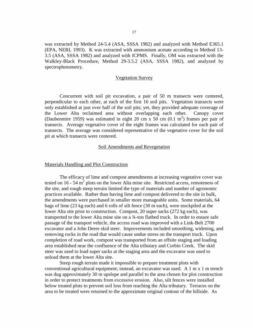
17
was extracted by Method 24-5.4 (ASA, SSSA 1982) and analyzed with Method E365.1
(EPA, NERL 1993). K was extracted with ammonium acetate according to Method 13-
3.5 (ASA, SSSA 1982) and analyzed with ICPMS. Finally, OM was extracted with the
Walkley-Black Procedure, Method 29-3.5.2 (ASA, SSSA 1982), and analyzed by
spectrophotometry.
Vegetation Survey
Concurrent with soil pit excavation, a pair of 50 m transects were centered,
perpendicular to each other, at each of the first 16 soil pits. Vegetation transects were
only established at just over half of the soil pits; yet, they provided adequate coverage of
the Lower Alta reclaimed area without overlapping each other. Canopy cover
(Daubenmire 1959) was estimated in eight 20 cm x 50 cm (0.1 m2) frames per pair of
transects. Average vegetative cover of the eight frames was calculated for each pair of
transects. The average was considered representative of the vegetative cover for the soil
pit at which transects were centered.
Soil Amendments and Revegetation
Materials Handling and Plot Construction
The efficacy of lime and compost amendments at increasing vegetative cover was
tested on 16 - 54 m2 plots on the lower Alta mine site. Restricted access, remoteness of
the site, and rough steep terrain limited the type of materials and number of agronomic
practices available. Rather than having lime and compost delivered to the site in bulk,
the amendments were purchased in smaller more manageable units. Some materials, 64
bags of lime (23 kg each) and 6 rolls of silt fence (30 m each), were stockpiled at the
lower Alta site prior to construction. Compost, 20 super sacks (272 kg each), was
transported to the lower Alta mine site on a ¾-ton flatbed truck. In order to ensure safe
passage of the transport vehicle, the access road was improved with a Link-Belt 2700
excavator and a John Deere skid steer. Improvements included smoothing, widening, and
removing rocks in the road that would cause undue stress on the transport truck. Upon
completion of road work, compost was transported from an offsite staging and loading
area established near the confluence of the Alta tributary and Corbin Creek. The skid
steer was used to load super sacks at the staging area and the excavator was used to
unload them at the lower Alta site.
Steep rough terrain made it impossible to prepare treatment plots with
conventional agricultural equipment; instead, an excavator was used. A 1 m x 1 m trench
was dug approximately 30 m upslope and parallel to the area chosen for plot construction
in order to protect treatments from excessive erosion. Also, silt fences were installed
below treated plots to prevent soil loss from reaching the Alta tributary. Terraces on the
area to be treated were returned to the approximate original contour of the hillside. As
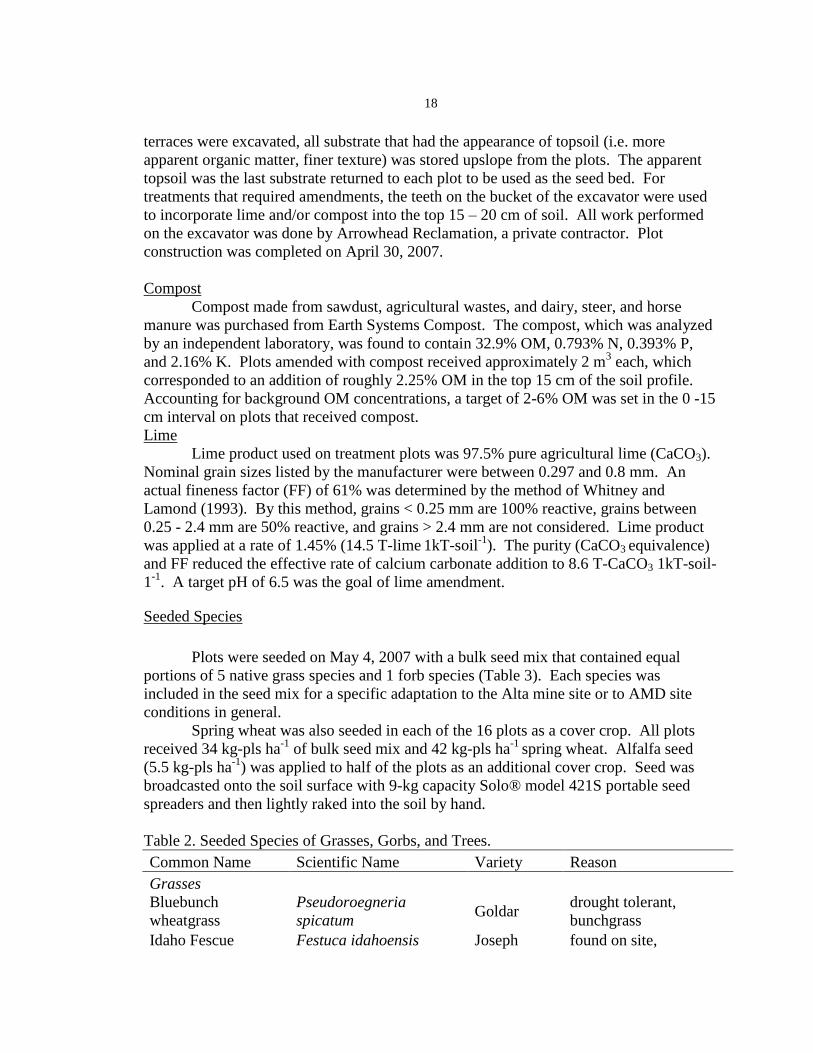
18
terraces were excavated, all substrate that had the appearance of topsoil (i.e. more
apparent organic matter, finer texture) was stored upslope from the plots. The apparent
topsoil was the last substrate returned to each plot to be used as the seed bed. For
treatments that required amendments, the teeth on the bucket of the excavator were used
to incorporate lime and/or compost into the top 15 – 20 cm of soil. All work performed
on the excavator was done by Arrowhead Reclamation, a private contractor. Plot
construction was completed on April 30, 2007.
Compost
Compost made from sawdust, agricultural wastes, and dairy, steer, and horse
manure was purchased from Earth Systems Compost. The compost, which was analyzed
by an independent laboratory, was found to contain 32.9% OM, 0.793% N, 0.393% P,
and 2.16% K. Plots amended with compost received approximately 2 m3 each, which
corresponded to an addition of roughly 2.25% OM in the top 15 cm of the soil profile.
Accounting for background OM concentrations, a target of 2-6% OM was set in the 0 -15
cm interval on plots that received compost.
Lime
Lime product used on treatment plots was 97.5% pure agricultural lime (CaCO3).
Nominal grain sizes listed by the manufacturer were between 0.297 and 0.8 mm. An
actual fineness factor (FF) of 61% was determined by the method of Whitney and
Lamond (1993). By this method, grains < 0.25 mm are 100% reactive, grains between
0.25 - 2.4 mm are 50% reactive, and grains > 2.4 mm are not considered. Lime product
was applied at a rate of 1.45% (14.5 T-lime 1kT-soil-1
). The purity (CaCO3 equivalence)
and FF reduced the effective rate of calcium carbonate addition to 8.6 T-CaCO3 1kT-soil-
1-1
. A target pH of 6.5 was the goal of lime amendment.
Seeded Species
Plots were seeded on May 4, 2007 with a bulk seed mix that contained equal
portions of 5 native grass species and 1 forb species (Table 3). Each species was
included in the seed mix for a specific adaptation to the Alta mine site or to AMD site
conditions in general.
Spring wheat was also seeded in each of the 16 plots as a cover crop. All plots
received 34 kg-pls ha-1
of bulk seed mix and 42 kg-pls ha-1
spring wheat. Alfalfa seed
(5.5 kg-pls ha-1
) was applied to half of the plots as an additional cover crop. Seed was
broadcasted onto the soil surface with 9-kg capacity Solo® model 421S portable seed
spreaders and then lightly raked into the soil by hand.
Table 2. Seeded Species of Grasses, Gorbs, and Trees.
Common Name Scientific Name Variety Reason
Grasses
Bluebunch
wheatgrass
Pseudoroegneria
spicatum Goldar
drought tolerant,
bunchgrass
Idaho Fescue Festuca idahoensis Joseph found on site,
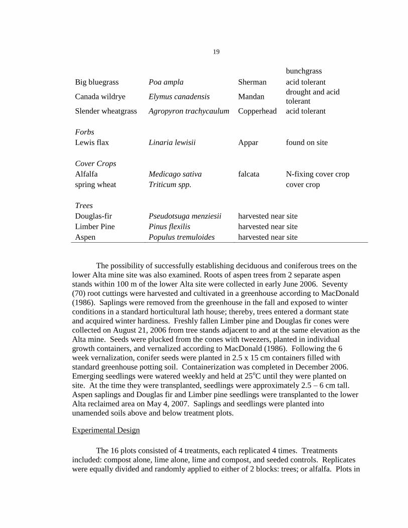
19
bunchgrass
Big bluegrass Poa ampla Sherman acid tolerant
Canada wildrye Elymus canadensis Mandan drought and acid
tolerant
Slender wheatgrass Agropyron trachycaulum Copperhead acid tolerant
Forbs
Lewis flax Linaria lewisii Appar found on site
Cover Crops
Alfalfa Medicago sativa falcata N-fixing cover crop
spring wheat Triticum spp. cover crop
Trees
Douglas-fir Pseudotsuga menziesii harvested near site
Limber Pine Pinus flexilis harvested near site
Aspen Populus tremuloides harvested near site
The possibility of successfully establishing deciduous and coniferous trees on the
lower Alta mine site was also examined. Roots of aspen trees from 2 separate aspen
stands within 100 m of the lower Alta site were collected in early June 2006. Seventy
(70) root cuttings were harvested and cultivated in a greenhouse according to MacDonald
(1986). Saplings were removed from the greenhouse in the fall and exposed to winter
conditions in a standard horticultural lath house; thereby, trees entered a dormant state
and acquired winter hardiness. Freshly fallen Limber pine and Douglas fir cones were
collected on August 21, 2006 from tree stands adjacent to and at the same elevation as the
Alta mine. Seeds were plucked from the cones with tweezers, planted in individual
growth containers, and vernalized according to MacDonald (1986). Following the 6
week vernalization, conifer seeds were planted in 2.5 x 15 cm containers filled with
standard greenhouse potting soil. Containerization was completed in December 2006.
Emerging seedlings were watered weekly and held at 25oC until they were planted on
site. At the time they were transplanted, seedlings were approximately 2.5 – 6 cm tall.
Aspen saplings and Douglas fir and Limber pine seedlings were transplanted to the lower
Alta reclaimed area on May 4, 2007. Saplings and seedlings were planted into
unamended soils above and below treatment plots.
Experimental Design
The 16 plots consisted of 4 treatments, each replicated 4 times. Treatments
included: compost alone, lime alone, lime and compost, and seeded controls. Replicates
were equally divided and randomly applied to either of 2 blocks: trees; or alfalfa. Plots in

20
the alfalfa block were seeded with bulk seed mix and an additional 5.5 kg pls ha-1
alfalfa.
The trees block received only the bulk seed mix; but the conifer seedlings and deciduous
saplings were planted in unamended soils around its perimeter (Figure 6).
Figure 5. Treatment Plot Layout for Experimental Revegetation Trials.
Quantification of Vegetative Cover
As was done in the baseline vegetation survey, canopy cover at the end of the
140-day growing season was measured with the Daubenmire method (1959). A single
diagonal transect from the southeast corner to the northwest corner of each treatment plot
was established. Cover was determined by species in 6 – 0.1 m2
frames spaced
approximately 1.8 m apart on each transect. Tree mortality was determined by counting
the number of living and dead trees at the end of the growing season.
Quantification of Soil Productivity
A composite soil sample from the amended soil depth was collected for each plot
from 4 locations, spaced approximately 2.7 m apart, on the diagonal transect. Samples
were collected in 1 L disposable cups and transferred to plastic bags. Samples were
homogenized by a thorough mixing within the plastic bags and during the drying process
of Sobek et al. (1978).

21
Soil samples derived from the treated plots were analyzed for OM, pH, EC, and
and water extractable Cd, Cu, Pb, Zn, and As. Methods of analysis were consistent with
those previously described except for OM and water extractable heavy metals and As.
OM was determined by the loss on ignition method (Nelson and Sommers 1996) because
it could be done cheaply in-house. Soils subject to loss on ignition (LOI) were ground
first, for 2 minutes in a SPEX Certiprep 8000D ball mill, with 1.27 cm diameter ceramic
balls. Water extractable heavy metals and As were determined from a 1:10 soil solution
because subsamples that remained after LOI were too small to yield a viable extract from
a 2:1 saturated paste; however, ICPMS was stilled used to determine heavy metal and As
concentrations.
Water Quality Monitoring
Surface Water Monitoring Locations
Paired stream flow measurements and sediment, As, and heavy metals samples
were collected at 6 surface water monitoring locations in both the Corbin Creek
watershed and Alta subwatershed throughout the summer of 2007 (Figure 7).
Figure 6. Summer 2007 Alta Sub-Watershed Surface Water Monitoring Locations.
The 6 sampling locations were: below the Upper Alta waste rock pile; at the #8
shaft; below the Lower Alta reclaimed area; above the confluence of the Alta tributary
and Corbin Creek (in the tributary); above the confluence of the Alta tributary and Corbin
Creek (in the creek); and below the confluence of the 2 streams. Monitoring locations in
the Alta tributary were situated in the approximate location described by Scroth (2001).
While the exact geographic location of 1999 and 2000 sample points was not known, the
locations proposed above are likely a close fit. The monitoring location in Corbin Creek
below the Alta tributary was situated well below the mixing zone (Thomann and Mueller
1987) determined by maximum stream velocity, depth, and width. Monitoring locations
allowed for comparison of 2007 As and heavy metal concentrations to heavy metal and
As concentrations present during reclamation (1999) and 1 year removed (2000). In
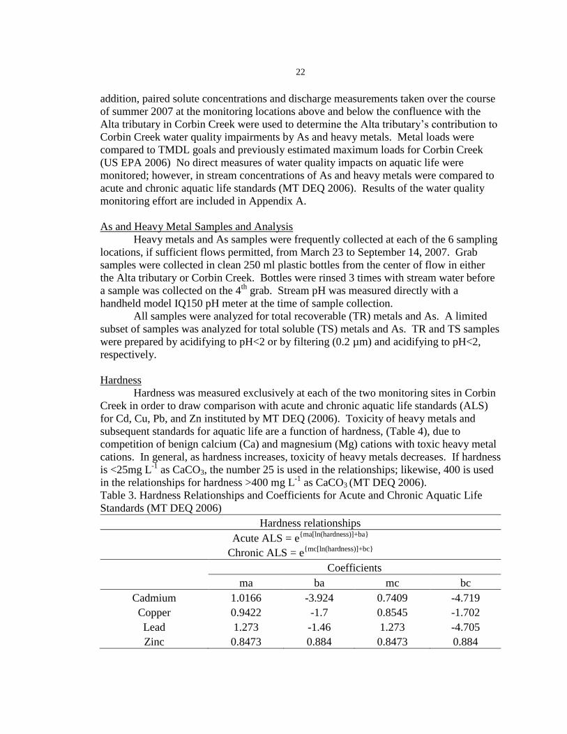
22
addition, paired solute concentrations and discharge measurements taken over the course
of summer 2007 at the monitoring locations above and below the confluence with the
Alta tributary in Corbin Creek were used to determine the Alta tributary’s contribution to
Corbin Creek water quality impairments by As and heavy metals. Metal loads were
compared to TMDL goals and previously estimated maximum loads for Corbin Creek
(US EPA 2006) No direct measures of water quality impacts on aquatic life were
monitored; however, in stream concentrations of As and heavy metals were compared to
acute and chronic aquatic life standards (MT DEQ 2006). Results of the water quality
monitoring effort are included in Appendix A.
As and Heavy Metal Samples and Analysis
Heavy metals and As samples were frequently collected at each of the 6 sampling
locations, if sufficient flows permitted, from March 23 to September 14, 2007. Grab
samples were collected in clean 250 ml plastic bottles from the center of flow in either
the Alta tributary or Corbin Creek. Bottles were rinsed 3 times with stream water before
a sample was collected on the 4th
grab. Stream pH was measured directly with a
handheld model IQ150 pH meter at the time of sample collection.
All samples were analyzed for total recoverable (TR) metals and As. A limited
subset of samples was analyzed for total soluble (TS) metals and As. TR and TS samples
were prepared by acidifying to pH<2 or by filtering (0.2 µm) and acidifying to pH<2,
respectively.
Hardness
Hardness was measured exclusively at each of the two monitoring sites in Corbin
Creek in order to draw comparison with acute and chronic aquatic life standards (ALS)
for Cd, Cu, Pb, and Zn instituted by MT DEQ (2006). Toxicity of heavy metals and
subsequent standards for aquatic life are a function of hardness, (Table 4), due to
competition of benign calcium (Ca) and magnesium (Mg) cations with toxic heavy metal
cations. In general, as hardness increases, toxicity of heavy metals decreases. If hardness
is <25mg L-1
as CaCO3, the number 25 is used in the relationships; likewise, 400 is used
in the relationships for hardness >400 mg L-1
as CaCO3 (MT DEQ 2006).
Table 3. Hardness Relationships and Coefficients for Acute and Chronic Aquatic Life
Standards (MT DEQ 2006)
Hardness relationships
Acute ALS = e{ma[ln(hardness)]+ba}
Chronic ALS = e{mc[ln(hardness)]+bc}
Coefficients
ma ba mc bc
Cadmium 1.0166 -3.924 0.7409 -4.719
Copper 0.9422 -1.7 0.8545 -1.702
Lead 1.273 -1.46 1.273 -4.705
Zinc 0.8473 0.884 0.8473 0.884

23
Hardness (as CaCO3) was determined by analysis of water samples for both Ca
and Mg cations by ICPMS. A single sample per month of study was randomly selected
for hardness determination and considered representative of hardness for the stream until
subsequent samples were taken.
Stream Gaging
The height of the water column was gaged at all surface water sampling locations
except for the #8 shaft and Corbin Creek above the Alta tributary. These sites were
excluded due to a limited number of gaging instruments and because the #8 shaft was not
a suitable location for instrumentation. Gage height was read with Ecotone WM water
level monitors at 15 minute intervals during the summer of 2007.
Discharge (Q) was determined at each monitoring location by 1 of 2 methods: 1) a
calibrated bucket and stopwatch; or 2) the continuity method and a Swoffer 3000 stream
velocity meter. As a rule, Q was determined by calibrated bucket at monitoring locations
at the lower Alta reclaimed site; and the velocity area method was used for sites lower in
the watershed. Sedimentation dams constructed at the lower Alta site in 1999 provided
confined flows over spillways that were easily sampled by calibrated bucket; further, rip
rap placed in the channel during the reclamation effort negated our ability to use a
velocity meter there. Monitoring locations at lower sites had no such spillways but were
free of large rocks that would preclude usage of a velocity meter. Gage heights were
related to stream flow by power function rating curves.
Suspended Sediment Samples and Analysis
Suspended sediment concentrations were monitored at each location except for
the #8 shaft. The height of the water column in both the Alta tributary and Corbin Creek
was insufficiently high to accommodate the use of standard USGS sampling equipment,
US DH-48 and US U-59 samplers. Instead, suspended sediment samples were collected
in an open bottle (US DH-48 variety), as suggested by Edwards and Glysson (1999).
Samples were analyzed according to standard methods (American Public Health
Association 1989) for Total Suspended Solids.
Precipitation
A tipping bucket rain gage with a Hobo® event recorder was deployed on
northeast corner of the lower Alta reclaimed site at approximately 1,710 m amsl. The
gage was situated on a level plane away from objects that would obstruct rain and wind.
The gage was used to record cumulative precipitation, event frequencies, and durations
from March 23 to October 1, 2007.
Snow Water Equivalent
Snow water equivalent was estimated in bi-weekly snow course measurements
from January 22 to April 15, 2007. Measurements were made according to Colbeck et al.
(1990) on a snow course established on the lower Alta reclaimed area. Slopes of south
and north aspect were represented in 10 established measuring locations within the snow
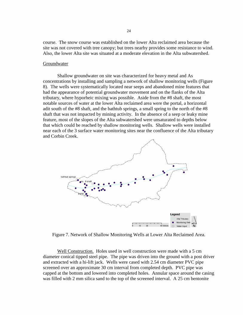
24
course. The snow course was established on the lower Alta reclaimed area because the
site was not covered with tree canopy; but trees nearby provides some resistance to wind.
Also, the lower Alta site was situated at a moderate elevation in the Alta subwatershed.
Groundwater
Shallow groundwater on site was characterized for heavy metal and As
concentrations by installing and sampling a network of shallow monitoring wells (Figure
8). The wells were systematically located near seeps and abandoned mine features that
had the appearance of potential groundwater movement and on the flanks of the Alta
tributary, where hyporheic mixing was possible. Aside from the #8 shaft, the most
notable sources of water at the lower Alta reclaimed area were the portal, a horizontal
adit south of the #8 shaft, and the bathtub springs, a small spring to the north of the #8
shaft that was not impacted by mining activity. In the absence of a seep or leaky mine
feature, most of the slopes of the Alta subwatershed were unsaturated to depths below
that which could be reached by shallow monitoring wells. Shallow wells were installed
near each of the 3 surface water monitoring sites near the confluence of the Alta tributary
and Corbin Creek.
Figure 7. Network of Shallow Monitoring Wells at Lower Alta Reclaimed Area.
Well Construction. Holes used in well construction were made with a 5 cm
diameter conical tipped steel pipe. The pipe was driven into the ground with a post driver
and extracted with a hi-lift jack. Wells were cased with 2.54 cm diameter PVC pipe
screened over an approximate 30 cm interval from completed depth. PVC pipe was
capped at the bottom and lowered into completed holes. Annular space around the casing
was filled with 2 mm silica sand to the top of the screened interval. A 25 cm bentonite

25
clay seal was layered over the sand in each well. Soils found on site were used to fill the
remainder of the annular space. Each well was capped with a 3.8 cm PVC sleeve to
prevent rainfall from entering the casing. Completed depths of the shallow wells ranged
from 114 cm to 200 cm below the ground surface.
Groundwater Sample Collection and Analysis. Shallow groundwater was drawn
from 12 of the monitoring wells in the summer of 2007. First, each well was purged with
a peristaltic pump to confirm a hydraulic connection with groundwater. Approximately 1
hour after purging, samples were pumped into clean 250 ml bottles from wells that
exhibited adequate recovery. The pH of each sample was measured with a handheld
Model IQ150 pH meter and recorded at the time of collection. Samples were filtered (0.2
μm), transferred to a separate clean sample bottle, and acidified to pH < 2. Samples were
analyzed by Energy Laboratories, Inc. of Billings, MT with inductively coupled plasma
mass spectroscopy (ICPMS).
Static Water Level Measurements. A Solinst® water level monitor was used to
establish groundwater depths below the ground surface. Water level measurements were
used to indicate water level recovery during groundwater sampling events. Also, bi-
monthly measurements were made throughout the summer of 2007.
Statistical Methods
Z* test Statistic
Existing soil As and Pb concentrations in the 0 – 15 cm interval were compared to
soil screening levels used in the 1999 reclamation project. The null hypothesis (Ho) was
that observed mean soil As and Pb levels were equivalent to targeted screening levels.
The alternative hypothesis (Ha) being that soil As and Pb concentrations in 2006 were
indeed higher than the screening levels. The hypothesis was tested on the basis of a Z
statistic (Devore and Farnum 2005). Prior to analysis, normal probability plots of the
data were examined and a logarithmic data transformation was made to normalize the
data.
ANOVA Approach to Linear Regression
Single and multifactor linear regression models were constructed in R 2.5.1 to
determine any correlation between soil physical and chemical properties and vegetation
on site. Vegetative cover was used as the dependent variable; and independent variables
included aspect, pH, ABP, OM, nutrients, heavy metals, and arsenic. Association
between dependent and independent variables was measured with the coefficient of
correlation (r); and regression models were considered significant at p<0.1. The aptness
of linear regression models was diagnosed with normal probability plots and plots of
residuals against fitted values. Significant single and restricted variable regression
models were compared to multifactor models by Analysis of Variance (ANOVA), using

26
R version 2.5.1 (2007), to account for variability in vegetation due to cumulative factor
effects. Like regression models, ANOVA models were considered significant at p<0.1.
Wilcoxon Rank Sum Test
The Wilcoxon Rank Sum Test was used to compare the relative quality of soil in
the 0 – 15 cm interval to that of soil in the 60 – 75 cm interval for each of the 30 soil pits.
The comparison was made on the basis of total Pb, As, Zn, OM, ABP, N, P, K, and pH.
It was expected that the test would establish patterns of incomplete waste removal,
upward movement of contaminants, or erosion of topsoil cover material.
The Wilcoxon Rank Sum Test was also used to compare lime and compost
treatment effectiveness at increasing pH, decreasing EC, increasing vegetative cover, and
decreasing available heavy metals and As. The test was used because the assumption of
normality was not appropriate with only 4 replicates of each treatment type. R 2.5.1 was
used to perform statistical computation.

27
RESULTS AND DISCUSSION
Water Quality Monitoring
Hydrograph
Stream flow in the Alta tributary and Corbin Creek was gaged and discharge
hydrographs for summer 2007 were approximated at three locations: at the lower Alta
reclaimed site, in the Alta tributary above Corbin Creek, and in Corbin Creek below the
Alta tributary (Figure 9). Low intermittent flows at the monitoring site between the
upper Alta waste rock dump and lower Alta reclaimed area prevented the establishment
of a hydrograph and limited the monitoring effort at that location. A discharge
hydrograph was not established for the #8 shaft, due to diffuse flows that were not
measurable by a calibrated bucket, stream velocity meter, or Ecotone® water level
monitor. As such, flows recorded at a confined overflow point 50 m downstream were
considered representative of #8 shaft discharge. Corbin creek above the Alta tributary
was not gaged; although, stream flow measurements were made as surface water samples
were collected. Surface water flows were not observed above the confluence with the
Alta tributary from 6/9/2007 to 9/14/2007.
Flow patterns in the Alta tributary immediately above Corbin Creek and in Corbin
Creek immediately below the tributary were typical of low order mountain steams. Peak
discharge at both sites corresponded to spring rain and snowmelt. Seasonal snow
accumulation had completely disappeared from the lower Alta snow course by early
April. Snow water equivalent accounted for 3.5 cm of the total 25.5 cm of precipitation
received in the Alta sub-watershed. At the lower Alta reclaimed site, discharge was
highly variable; and flow patterns were controlled more by mine shaft discharge than by
surface hydrologic processes. Discharge at all locations was low and easily quantified in
L min-1
. Peak flow at all sites occurred on May 22, as the result of an extended late
spring rainfall event. Peak flows were estimated as 239, 137, and 91 L min-1
,
respectively, at Corbin Creek below Alta, the Alta tributary above Corbin Creek, and at
the lower Alta reclaimed site.

28
Figure 8. Rainfall Hyetograph, Snow Water Equivalent, and Mean Daily Discharge for
A.) Corbin Creek Below the Alta Tributary, B.) Alta Tributary Above Corbin Creek, C.)
Alta Tributary Below Lower Alta Reclaimed Area.
Surface Water pH
Each monitoring location had a distinct pH signature. Generally, pH was greatest
in surface flows of Corbin Creek above the confluence with the Alta tributary.
Measurements made at the upper Corbin Creek monitoring location ranged from 7.16 –
8.0 before the stream dried up in early June 2007. Neutral pH at this site might be the
result of lime applied to soils and limestone rip-rap used in the stream channel during the
reclamation of the Bertha tailings. This is a crude indicator that removal of the acidic
tailings (pH < 3.0, Deckler 1982) may have mitigated water quality impacts in Corbin
Creek above the contribution of the Alta tributary.
Stream flow at all other monitoring locations exhibited pH that was well below
neutral. A single pH measurement of the intermittent surface flow between the upper
Alta waste rock pile and lower Alta reclaimed site was 3.5. Trends in pH followed the

29
hydrograph at the remainder of the monitoring locations (Figure 10). Generally, pH was
highest for observations made in the spring and during precipitation events. When peak
hydrograph conditions subsided in early June, a distinct drop in pH was observed at all
locations. The pH drop was likely attributable to less mixing with neutral snow-melt and
shallow meteoric waters.
Decreased pH was nowhere more noticeable than in Corbin Creek below Alta,
where pH dropped by more than 1 unit (from 3.7 to 2.5). The decrease in pH at this
location was due to vanished or reduced mixing with neutral surface waters from above.
Discharge from the #8 shaft had the highest pH (as high as 4.63) of the monitoring
locations in the Alta tributary; but it decreased rapidly in the downstream direction. The
rapid decrease was probably due to sulfide oxidation or the precipitation of Fe-
hydroxides. The stream channel immediately below the #8 shaft was blanketed with
ferric hydroxide precipitates. It was common for pH to have dropped more than 1 unit by
the time flows exited the lower Alta reclaimed site, roughly 180 m downstream. Further
reductions in pH occurred in the downstream direction. Surface flows with the lowest pH
were generally found in the Alta tributary immediately above Corbin Creek.
2
3
4
5
4/22
/2007
5/6/
2007
5/20
/2007
6/3/
2007
6/17
/2007
7/1/
2007
7/15
/2007
7/29
/2007
8/12
/2007
8/26
/2007
9/9/
2007
Date
pH
#8 Shaft Alta Reclaimed Area
Alta above Corbin Corbin below Alta
Figure 9. Temporal Trends in Alta Sub-Watershed pH by Site.
Heavy Metals and As.
Sources of heavy metal and arsenic varied by element and were controlled by pH,
stream flow patterns, and apparent reactive processes. Heavy metal and As monitoring
was only meaningful at or below the #8 shaft. Intermittent stream flow between the
upper Alta waste rock pile and lower Alta reclaimed area was minimal during visits to the
site. Before the flows ceased in early June 2007, two (2) observations of paired flow and
heavy metal and As concentrations were made at the monitoring location between the
upper and lower Alta (Table 5). Loads greater than those observed were likely to have
occurred during peak runoff and high intensity rainfall events; but low aqueous metal and

30
As concentrations would still result in significantly lower transport rates than those
measured at downstream monitoring locations.
Table 4. Heavy Metal and Arsenic Loads From Upper Alta Waste Rock Pile.
Element Load kg day-1
Date Time Flow
M/DD HH:MM L min-1
As Cd Cu Pb Zn
23-Mar 16:00 8.18 ND* ND* 0.12 0.04 0.62
22-Apr 13:00 1.57 0.07 0.005 0.18 0.33 5.04
*ND=Element not detectable by ICPMS
Arsenic was predominately discharged from the #8 shaft and was naturally
attenuated in the downstream direction (Figure 11). As concentrations observed in the #8
shaft discharge ranged from 4.37 – 10.5 mg L-1
but decreased by an average of 73% at
the monitoring location approximately 180 m downstream. Enriched As concentrations
in #8 shaft discharge resulted in the highest loads of any site in the Alta tributary. Stream
flow increased in the downstream direction from March to June; so dilution may have
accounted for some of the decrease in As concentration. However, the decline in As load
was likely due to co-precipitation with noticeable Fe-hydroxides in the channel of the
lower Alta reclaimed site. No measures of Fe-hydroxide production or As sorption were
made in the monitoring effort.
0
0.2
0.4
0.6
0.8
1
1.2
3/23
/07
4/23
/07
5/24
/07
6/24
/07
7/25
/07
8/25
/07
Date
As
(k
g d
ay
-1)
#8 Shaft Alta Reclaimed Area
Above Corbin Creek Corbin Creek Below Alta
Figure 10. Temporal Trend in Alta Sub-Watershed As Loads by Site.
Cu load in the tributary was similar in magnitude to As load; but it exhibited an
opposite trend (Figure 12). Concentrations emerging from the #8 shaft were 0.1 – 0.3 mg
Cu L-1
during spring and early summer and no Cu was observed in shaft discharge (by
ICPMS) from June 11 to September 14, 2007. Cu load increased in the downstream
direction, which implicated an input of leachate from Alta mine soils or waste rock in the
lower reach of the tributary. The highest Cu loads were typically measured at the Alta
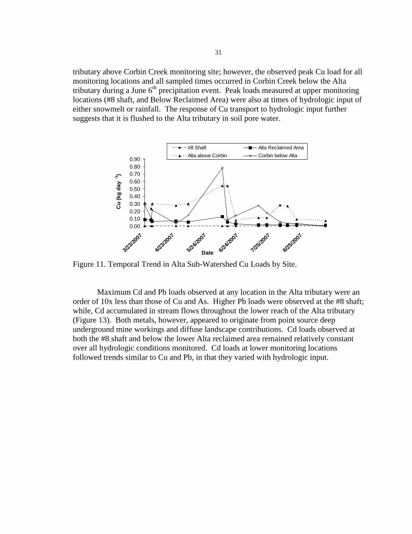
31
tributary above Corbin Creek monitoring site; however, the observed peak Cu load for all
monitoring locations and all sampled times occurred in Corbin Creek below the Alta
tributary during a June 6th
precipitation event. Peak loads measured at upper monitoring
locations (#8 shaft, and Below Reclaimed Area) were also at times of hydrologic input of
either snowmelt or rainfall. The response of Cu transport to hydrologic input further
suggests that it is flushed to the Alta tributary in soil pore water.
0.00
0.10
0.20
0.30
0.40
0.50
0.60
0.70
0.80
0.90
3/23
/200
7
4/23
/200
7
5/24
/200
7
6/24
/200
7
7/25
/200
7
8/25
/200
7
Date
Cu
(k
g d
ay
-1)
#8 Shaft Alta Reclaimed Area
Alta above Corbin Corbin below Alta
Figure 11. Temporal Trend in Alta Sub-Watershed Cu Loads by Site.
Maximum Cd and Pb loads observed at any location in the Alta tributary were an
order of 10x less than those of Cu and As. Higher Pb loads were observed at the #8 shaft;
while, Cd accumulated in stream flows throughout the lower reach of the Alta tributary
(Figure 13). Both metals, however, appeared to originate from point source deep
underground mine workings and diffuse landscape contributions. Cd loads observed at
both the #8 shaft and below the lower Alta reclaimed area remained relatively constant
over all hydrologic conditions monitored. Cd loads at lower monitoring locations
followed trends similar to Cu and Pb, in that they varied with hydrologic input.
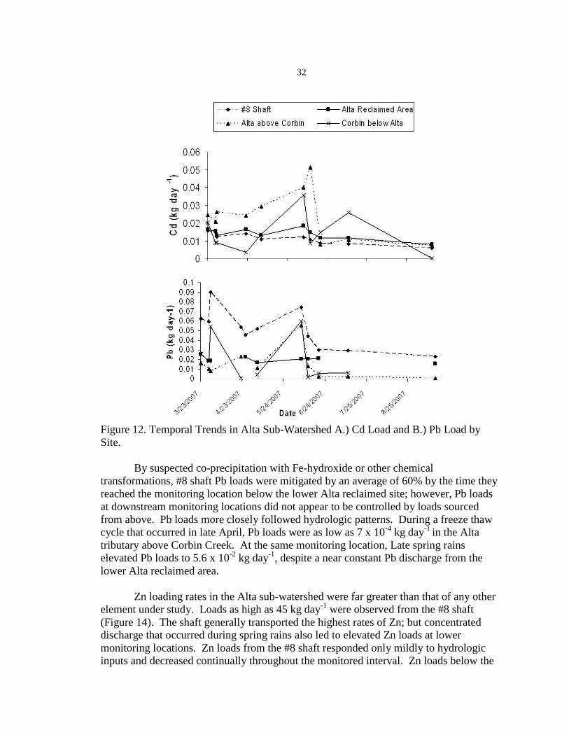
32
Figure 12. Temporal Trends in Alta Sub-Watershed A.) Cd Load and B.) Pb Load by
Site.
By suspected co-precipitation with Fe-hydroxide or other chemical
transformations, #8 shaft Pb loads were mitigated by an average of 60% by the time they
reached the monitoring location below the lower Alta reclaimed site; however, Pb loads
at downstream monitoring locations did not appear to be controlled by loads sourced
from above. Pb loads more closely followed hydrologic patterns. During a freeze thaw
cycle that occurred in late April, Pb loads were as low as 7 x 10⁻⁴
kg day-1
in the Alta
tributary above Corbin Creek. At the same monitoring location, Late spring rains
elevated Pb loads to 5.6 x 10⁻²
kg day-1
, despite a near constant Pb discharge from the
lower Alta reclaimed area.
Zn loading rates in the Alta sub-watershed were far greater than that of any other
element under study. Loads as high as 45 kg day-1
were observed from the #8 shaft
(Figure 14). The shaft generally transported the highest rates of Zn; but concentrated
discharge that occurred during spring rains also led to elevated Zn loads at lower
monitoring locations. Zn loads from the #8 shaft responded only mildly to hydrologic
inputs and decreased continually throughout the monitored interval. Zn loads below the

33
lower Alta reclaimed area were relatively constant throughout the study and did not
decrease with decreasing Zn input from the #8 shaft above.
05
101520253035404550
3/23
/07
4/22
/07
5/22
/07
6/21
/07
7/21
/07
8/20
/07
Date
Zn
(k
g d
ay-1
)
#8 Shaft Below Reclaimed area
Above Corbin Creek Corbin Creek below Alta
Figure 13. Temporal Trends in Alta Sub-Watershed Zn Load by Site.
Heavy Metals and As in Soil-Water and Groundwater.
Concentrations of As, Cu, and Zn were determined in both soil-water and in
shallow groundwater for a random sub-sample of soil pits and monitoring wells,
respectively, on the lower Alta reclaimed area in order to determine the contribution of
the elements from the mine-impacted landscape. Groundwater samples were collected on
August 17th
and limited to wells constructed at the lower Alta reclaimed area because
wells at the Corbin Creek and Alta tributary above Corbin Creek monitoring locations
were dry at the time of sampling. Soil and groundwater source determination was
particularly important in the case of Cu loading to the Alta tributary, as the #8 shaft was
found to be a minimal source of that element. By examination of surface water
concentrations of other heavy metals, it appeared that Cd, Pb, and Zn came from both
deep underground sources and landscape sources. Zn was the only of the three metals
measured in soils and groundwater; and its behavior was treated as a surrogate for Cd and
Pb behavior. As concentrations in soil and shallow groundwater were determined to test
the assumption that As was primarily discharged from the #8 shaft and because As
behaves markedly different in soil and aqueous systems than heavy metals (Inskeep et al.
2002).
Patterns of soil-water and shallow groundwater As, Cu, and Zn concentrations
differed greatly by element (Figure 15). Maximum water extractable Zn concentrations
in soil were lower than groundwater concentrations or surface water quantities at either
the #8 shaft or below the lower Alta reclaimed area; but considerably higher than soil
water concentrations of the other elements. On the date sampled, Zn concentrations at
the shaft and below the reclaimed area were nearly equal. Shallow groundwater Zn
concentrations in wells immediately adjacent to the Alta tributary were indicative of
concentrated surface waters mixing with dilute soil leachate that had accumulated in the
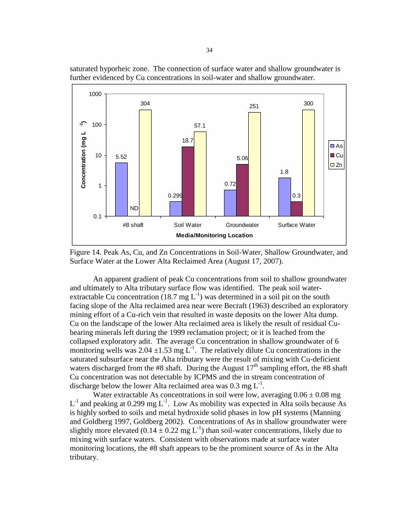
34
saturated hyporheic zone. The connection of surface water and shallow groundwater is
further evidenced by Cu concentrations in soil-water and shallow groundwater.
5.52
0.299
0.72
1.8
18.7
5.06
0.3
304
57.1
251 300
0.1
1
10
100
1000
#8 shaft Soil Water Groundwater Surface Water
Media/Monitoring Location
Co
ncen
trati
on
(m
g L
-1)
As
Cu
Zn
ND
Figure 14. Peak As, Cu, and Zn Concentrations in Soil-Water, Shallow Groundwater, and
Surface Water at the Lower Alta Reclaimed Area (August 17, 2007).
An apparent gradient of peak Cu concentrations from soil to shallow groundwater
and ultimately to Alta tributary surface flow was identified. The peak soil water-
extractable Cu concentration (18.7 mg L-1
) was determined in a soil pit on the south
facing slope of the Alta reclaimed area near were Becraft (1963) described an exploratory
mining effort of a Cu-rich vein that resulted in waste deposits on the lower Alta dump.
Cu on the landscape of the lower Alta reclaimed area is likely the result of residual Cu-
bearing minerals left during the 1999 reclamation project; or it is leached from the
collapsed exploratory adit. The average Cu concentration in shallow groundwater of 6
monitoring wells was 2.04 ±1.53 mg L-1
. The relatively dilute Cu concentrations in the
saturated subsurface near the Alta tributary were the result of mixing with Cu-deficient
waters discharged from the #8 shaft. During the August 17th
sampling effort, the #8 shaft
Cu concentration was not detectable by ICPMS and the in stream concentration of
discharge below the lower Alta reclaimed area was 0.3 mg L-1
.
Water extractable As concentrations in soil were low, averaging 0.06 ± 0.08 mg
L-1
and peaking at 0.299 mg L-1
. Low As mobility was expected in Alta soils because As
is highly sorbed to soils and metal hydroxide solid phases in low pH systems (Manning
and Goldberg 1997, Goldberg 2002). Concentrations of As in shallow groundwater were
slightly more elevated (0.14 ± 0.22 mg L-1
) than soil-water concentrations, likely due to
mixing with surface waters. Consistent with observations made at surface water
monitoring locations, the #8 shaft appears to be the prominent source of As in the Alta
tributary.
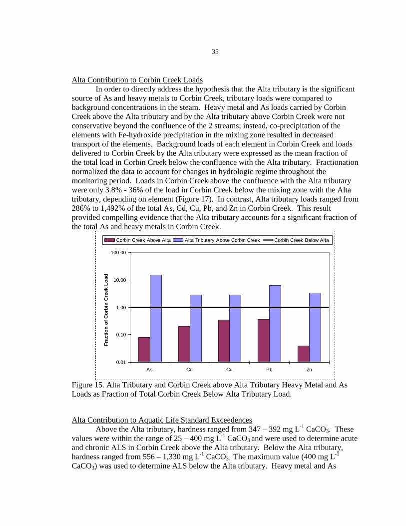
35
Alta Contribution to Corbin Creek Loads
In order to directly address the hypothesis that the Alta tributary is the significant
source of As and heavy metals to Corbin Creek, tributary loads were compared to
background concentrations in the steam. Heavy metal and As loads carried by Corbin
Creek above the Alta tributary and by the Alta tributary above Corbin Creek were not
conservative beyond the confluence of the 2 streams; instead, co-precipitation of the
elements with Fe-hydroxide precipitation in the mixing zone resulted in decreased
transport of the elements. Background loads of each element in Corbin Creek and loads
delivered to Corbin Creek by the Alta tributary were expressed as the mean fraction of
the total load in Corbin Creek below the confluence with the Alta tributary. Fractionation
normalized the data to account for changes in hydrologic regime throughout the
monitoring period. Loads in Corbin Creek above the confluence with the Alta tributary
were only 3.8% - 36% of the load in Corbin Creek below the mixing zone with the Alta
tributary, depending on element (Figure 17). In contrast, Alta tributary loads ranged from
286% to 1,492% of the total As, Cd, Cu, Pb, and Zn in Corbin Creek. This result
provided compelling evidence that the Alta tributary accounts for a significant fraction of
the total As and heavy metals in Corbin Creek.
0.01
0.10
1.00
10.00
100.00
As Cd Cu Pb Zn
Fra
cti
on
of
Co
rbin
Cre
ek L
oad
Corbin Creek Above Alta Alta Tributary Above Corbin Creek Corbin Creek Below Alta
Figure 15. Alta Tributary and Corbin Creek above Alta Tributary Heavy Metal and As
Loads as Fraction of Total Corbin Creek Below Alta Tributary Load.
Alta Contribution to Aquatic Life Standard Exceedences
Above the Alta tributary, hardness ranged from 347 – 392 mg L-1
CaCO3. These
values were within the range of 25 – 400 mg L-1
CaCO3 and were used to determine acute
and chronic ALS in Corbin Creek above the Alta tributary. Below the Alta tributary,
hardness ranged from 556 – 1,330 mg L-1
CaCO3. The maximum value (400 mg L-1
CaCO3) was used to determine ALS below the Alta tributary. Heavy metal and As

36
concentrations measured in the summer of 2007 were compared to ALS established for
each element (Figure 18).

37
Figure 16. Heavy Metal and As Concentrations in Corbin Creek Above and Below the
Alta Tributary Compared to Aquatic Life Standards in Summer of 2007.
Trace element concentrations that exceeded acute and chronic ALS were common
at both monitoring locations in Corbin Creek for all elements with the exception of As.
Only below the confluence with the Alta tributary were exceedances of ALS observed in
the summer of 2007. Exceedances of only the chronic ALS, which is the lower standard,
were observed at the monitoring location in Corbin Creek below the Alta tributary. This
result suggests that of all of the elements considered in this study, As may have the least
amount of impact on the health of aquatic life.
All observed heavy metal concentrations in Corbin Creek at monitoring locations
above and below the Alta tributary exceeded at least the chronic ALS. Pb was the only
metal not concentrated at levels above the acute ALS for all observations made. Even so,
Pb was concentrated to levels above the acute ALS during early spring runoff. The level
of exceedance for Cd, Cu, Pb, and Zn was far greater below the Alta tributary than in
Corbin Creek above, as evidenced by the y-axes in the plot above. Again, the greater
exceedances can be attributed to the disproportionately large loads contributed by the
Alta tributary.
Alta Contribution to TMDL Exceedances
As and heavy metal loading rates measured in Corbin Creek above and below the
Alta tributary were also compared directly to Corbin Creek TMDLs. Loads measured in
the summer of 2007 at both of the Corbin Creek monitoring sites were plotted with the
envelope of TMDL goals and previously estimated maximum daily loads (US EPA 2006)
(Figure 19). Patterns of TMDL exceedances varied by element; but more and greater
exceedances were observed in Corbin Creek below the Alta tributary. Pb and As loads
exceeded the TMDL only during observed periods of high flow and only in Corbin Creek
below the Alta tributary; although, Pb loads in Corbin Creek above the Alta tributary
were very near the TMDL during periods of high flow. Like Pb and As, Zn loads only
exceeded the TMDL in Corbin Creek below the Alta tributary. There, Zn loads routinely,
almost daily, exceeded the TMDL under all hydrologic conditions.

38
Figure 17. Corbin Creek Heavy Metal and As Loads Above and Below the Alta Tributary
Compared to TMDL Goals and EPA Estimated Maximum Loads (US EPA 2006).
The plots provide evidence that TMDLs were not often exceeded by Corbin Creek
background As and heavy metal concentrations alone; but that the Alta tributary
contribution to Corbin Creek resulted in loads that exceeded TMDLs during some or all
hydrologic conditions. Cu and Cd loads measured above the Alta tributary during the
greatest observed flow events were the only exceptions. The combined results of the Alta
tributary load to Corbin Creek background load comparison, ALS comparison, and
TMDL comparison provide evidence to accept the hypothesis that the Alta tributary is
not only the significant source of heavy metals and As but that it hinders attainment of
TMDLs.
Sediment
Sediment transport, estimated by total suspended solids (TSS), was lower than
estimated daily maxima for Corbin Creek (US EPA 2006) throughout the summer at all
monitoring locations. The highest sediment loading rates observed came during the June
39
6, 2007 rainfall event or early spring runoff measured on March 30, 2007 (Table 6).
Concentrations of TSS measured during low flow or baseflow conditions were often
below the detectable limit of the analytical method (APHA 2001). Difficulties in
determining suspended sediment concentrations below the lower Alta reclaimed area
arose because Fe rapidly precipitated in sample bottles before samples could be
transported to the lab; thus, the analysis of suspended sediment was restricted to the Alta
tributary above Corbin Creek and Corbin Creek above and below the Alta tributary.
Table 5. Summer 2007 Alta Tributary and Corbin Creek Sediment Loads and TMDLs.
TMDL
EPA Estimated
Maximum
Measured
Maximum
Monitoring Location kg day-1
kg day-1
kg day-1
Corbin Creek Below Alta 0.45 0.59 0.065
Corbin Creek Above Alta 0.45 0.59 0.037
Alta Tributary Above Corbin Creek -- -- 0.018
No TMDL exceedances were measured at either of the Corbin Creek monitoring
locations. Also, the maximum observed sediment load carried by the Alta tributary was
not above the TMDL established for Corbin Creek. During the monitoring effort,
substantial accumulation of sediment was observed behind each of the sediment traps
installed during the 1999 Alta reclamation project and the 2002 Bertha tailings removal.
It is likely that sediment aggradation is the result of debris flows from low frequency high
intensity rainfall events (Benda 1990) that occurred without observation or prior to the
study. More monitoring data that includes these events are needed to construct a new
sediment transport model or to validate the existing one (US EPA 2006) in Corbin Creek
below the Confluence with the Alta tributary.
Soil Characterization
Soil physical and chemical factors were successfully analyzed as outlined in
methods and materials. A summary of the results of the soil survey are presented below.
Complete results are listed in Appendix B. Where applicable, soil parameters in subsoil
were compared to parameters in topsoil on the basis of the Wilcoxon Rank Sum Test.
Soil Texture
All soils analyzed for texture, from both the surface and at depth, were found to be
either sandy loam or loamy sand. Sand, silt, and clay fractions ranged from 56.1 – 84 %,
8 – 42.5 %, and 0 – 15.6 %, respectively. Rock fragments (> 2 mm) ranged from 24 – 70
% by mass of each sample. The texture, rock content, elevation, and appearance of Alta
soils are consistent with the Comad series (Veseth and Montagne 1980) of well-drained,
weak-structured, granitic soils. Soils of this type may be limiting to a revegetation effort
because of their high erodability and inability to hold moisture.

40
Soil Nutrients and Organic Matter
Soil fertility on the basis of N was typically low on the Alta reclaimed site; and P
levels were low to medium (Table 7). K concentrations were near or below the range for
disturbed soils (150 mg kg-1
– 500 mg kg-1
); and OM was found to be in the low (2.1 –
3.5 %) to very low (<2 %) range (Munshower 1994). The lack of N and P in Alta soils
may be explained conceptually by a cumulative effect of their low OM and coarse
texture. Nutrients are leached from the well-drained soils when there is not sufficient
OM to bind them. Sterile soils will not support vegetation; thus, they will not receive
input of additional OM due to natural plant decay. Eventually, the structureless bare soils
will erode. Merely through the textural and nutrient analyses of Alta soils, there was
impetus for soil amendment with OM.
Table 6. Nutrient (mg kg-1
) concentrations and OM (%) in Alta mine soils
Macronutrient
Interval Nitrate (N) P-Olsen K-extractable OM
0 - 15 cm 2.6 ± 1.07 a 11.1 ± 5.7 a 107.3 ± 41.2 a 2.046 ± 0.84 a
60 - 75 cm 2 ± 1.6 a 14.7 ± 7.8 a 63.7 ± 26.4 b 1.33 ± 0.5 b
Values followed by same letter within columns are not significantly different (p<0.1).
pH and EC
The pH of Alta soils ranged from 2.32 – 7.23 in the 0-15 cm interval and from
2.53 – 6.21 in the 65 – 70 cm interval. More instances of near neutral pH occurred in the
upper interval, which is indicative of remnants of topsoil from the 1999 reclamation
effort. Overall, pH of surface soils was significantly greater than that of subsoils (Table
8); however, many soil samples in both intervals were in the range of acute toxicity to
plants (Rengel 2002).
Table 7. pH (standard units) and EC (μS cm-1
) of Alta mine soils.
Interval pH EC
0 - 15 cm 4.45 ± 1.2 a 535.8 ± 491.1 a
60 - 75 cm 3.45 ± 0.9 b 854 ± 546.7 b
Values followed by same letter within columns are not significantly different (p<0.1).
By EC measurement, salinity of Alta soils was found to be sufficiently lower than
published inhibitory thresholds. Depending on species, salinity is not expected to cause a
reduction in yield of grass or other forage except at levels > 2,300 µS/cm (Cardon et al
2003). EC was lower in surface samples than at depth, which suggested that plant
exposure to salts is limited. The low level of available salts may only prove to be
significant if they contain phytotoxic trace elements. Salts of CdCl+ were increasingly
taken up by wheat and Swiss chard (Beta vulgaris) when dissolved NaCl salts were added
to soil solution (Weggler-Beaton et al. 2000).

41
Heavy Metals and Arsenic
Total Metals and Arsenic. Prior to reclamation in 1999, mean Pb and As
concentrations in the top 75 cm of waste were 3,238 mg kg-1
and 1,063 mg kg-1
,
respectively (PRC EMI 1997). In the reclaimed condition, respective mean
concentrations over the entire 75 cm interval were reduced to 373 mg Pb kg-1
and 337 mg
As kg-1
. The mean Zn concentration of Alta waste from 3 samples taken in 1993 was 300
mg kg-1
(Pioneer 1994), which was actually lower than mean Zn concentrations found in
30 soil pits in summer of 2006. Concentrations of total metals and As in Alta mine
surface soils were not significantly different than concentrations at depth (Table 9). It is
possible that metals have either migrated from mine impacted subsoils into the more
recently applied topsoil by capillarity or that topsoil cover has been removed by erosion.
Table 8. Heavy metals and As (mg kg -1
) in Alta mine soils.
Heavy Metals and As
Interval As Pb Zn Total
0 - 15 cm 316.8 ± 473.8 a 355.7 ± 304.9 a 391.9 ± 120.6 a 1,064.4 ± 756 a
60 - 75 cm 357 ± 336.3 a 390.6 ± 398.3 a 440.3 ± 234 a 1187.9 ± 614 a
Values followed by same letter within columns are not significantly different (p<0.1).
Target removal concentrations of Pb and As used in the 1999 reclamation effort
were 235 mg kg-1
and 323 mg kg-1
, respectively (PRC-EMI 1997). This means that the
waste rock pile was removed until surface concentrations were routinely at or below
targets. Once target levels were reached, removal ceased. Current soil As and Pb
concentrations in the 0 – 15 cm interval were tested against reclamation targets, assuming
a lognormal distribution and a Z* test statistic. The null hypothesis of the test was that
mean soil concentrations were equal to target concentrations; conversely, the alternative
hypothesis was that surface soil concentrations were higher than targets. Though Pb and
As levels in surface soils were indicative of mine impacted materials, neither element was
significantly (p<0.1) concentrated above target levels (Table 10).
Table 9. Recreational clean up levels and current Pb and As in Alta mine soils.
Comparison to Reclamation Targets
Element Target mg
kg-1
mean ± standard deviation
mg kg-1
Z* p
As 323 316.8 ± 473.8 -3.474 0.9997
Pb 235 355.7 ± 304.9 0.694 0.25
Soluble Metals and Arsenic. Water extractable Cu, As, and Zn concentrations
were determined for a random subset of soils in the 0 – 15 cm interval, as this was the
primary rooting depth observed during soil pit excavation. The soluble fraction of these
constituents is not only indicative of bioavailability but also of the amount of potentially
toxic trace elements that may migrate from soil to surface and ground water.
Concentrations were variable but higher for Cu and Zn than for As. Concentrations
42
ranged from 0.07 – 18.7 mg L-1
and 0.01 – 57.1 mg L-1
for Cu and Zn, respectively.
Water soluble As concentrations ranged from non detectable by ICPMS to 0.299 mg L-1
.
Acid-Base Potential
ABP was measured in the 0 – 15 cm interval for all 30 soil pits and in the 60 – 75
cm interval for 7 soil pits. The Wilcoxon Rank Sum Test was used to draw comparison
between intervals. There was not a significant difference (p<0.1) between ABP in
surface soils and ABP at depth. In the 0 -15 cm depth interval, ABP ranged from net acid
neutralizing (13 T-CaCO3 1kT-soil-1-1
) to net acid producing (-57 T-CaCO3 1kT-soil-1
),
with a mean value of -4.23 T-CaCO3 kT-soil-1
. ABP from 8 T-CaCO3 kT-soil-1
to -45 T-
CaCO3 kT-soil-1
were found in the 60 – 75 cm soil interval. Prior to waste rock removal
in 1999, the top 75 cm of waste rock had ABP ranging from -12 T-CaCO3 1kT-soil-1-1
to
-196 T-CaCO3 1kT-soil-1-1
(PRC EMI 1997). Though soils at the Alta mine appeared to
have less acid generating potential than extreme values present in pre-reclamation
substrates, net acid producing values of ABP indicated that low soil pH at the Alta mine
may yet be the result of active sulfide mineral weathering.
Vegetation Survey
Vegetative cover on the Alta reclaimed site was generally sparse. Mean
vegetative cover determined from all sample frames was 11.7 %; yet, it ranged from 0 –
67.5 %. On the slope of north aspect, mean vegetative cover was 21.6 %, as compared to
only 6.1 % on south facing slopes. Bare ground, rocks, and litter were abundant on site.
Together, they accounted for a minimum of 40 % or 45 % of the total area in any given
sample frame on the north or south facing slope, respectively. Much of the sampled area
on the south facing slope was 95 – 100 % bare. Despite having minimal vegetative
cover, 31 different plant species were identified on site (Table 11).
The Alta reclaimed area, with relatively high species richness and low vegetative
cover, does not correspond with patterns of vegetative establishment on 3 reclaimed
mines nearby. Tafi (2006) found only 12 species on a reclaimed site with 38.1 % cover
and 37 species in an area with 70.9 % cover. Of the 31 species found at Alta, 20 were
native and only 12 were seeded during the 1999 reclamation effort. Complete results of
the vegetation survey are tabulated in Appendix B.

43
Table 10. Plant Species Found 7 Years After Reclamation of Alta Mine.
Common Name Scientific Name
Native 1999 Seed Mix
Y/N Y/N
Western Yarrow Achillea millifolium Y Y
Thickspike wheatgrass Agropyron dasystachyum Y Y
Intermdiate wheatgrass Agropyron intermedium N N
Western wheatgrass Agropyron smithii Y N
Slender wheatgrass Agropyron trachycaulum Y N
Redtop Agrostis alba N Y
Ticklegrass Agrostis scrabra N N
Fringed sagewort Artemesia frigeria Y N
Aster Aster spp Y N
Cheatgrass Bromus tectorum N N
Wavyleaf thistle Cirsium undulatum Y N
Idaho fescue Festuca idahoensis Y Y
Sheep fescue Festuca ovina Y N
Rough fescue Festuca scabrella Y Y
Hawk's beard Hierceulum Y N
Dalmation toadflax Linaria dalmatica N N
Lewis flax Linaria lewisii Y Y
Annual ryegrass Lolium multiflorum N Y
Silky Lupine Lupinus sericeus Y N
Alfalfa Medicago sativa N Y
Canada bluegrass Poa compressa N Y
Kentucky bluegrass Poa pratensis N N
Sandberg bluegrass Poa sandbergii Y Y
American bistort Polygonum bistortoides Y N
Quaking aspen Populus tremuloides Y N
Bluebunch wheatgrass Pseudoroegneria spicatum Y Y
Raspberry Rubus Y N
Columbia needlegrass Stipa columbiana Y Y
Green needlegrass Stipa viridula Y N
Western salsify Tragopogon dubius N N
Mullen Verbascum thapsus N N
Correlation between Soil and Vegetative Cover
Univariate and multifactor linear regression models were constructed in R 2.5.1 to
determine correlation between soil physical and chemical properties and vegetative
cover. Results of all linear regression models, including correlation coefficients, p-
values, and diagnostics plots are included in Appendix B.

44
Univariate Models
Single variable models found significantly correlated with vegetative cover were
pH (0 – 15 cm), EC (60 – 75 cm), P (60 – 75 cm), soluble As (0 – 15 cm), and aspect
(Table 12). EC and aspect were negatively correlated; while, pH, P, and As were
positively correlated with vegetative cover.
Table 11. Significant Models for Vegetative Cover on Lower Alta Reclaimed Site.
Results Model Coefficient Intercept r p
Cover ~ As, soluble (0-15cm interval) 108.193 6.145 0.84 0.00058
Cover ~ Aspect -9.36 16.071 -0.49 0.05434
Cover ~ EC (60-75cm interval) -0.01183 18.587 -0.54 0.02987
Cover ~ P (60-75cm interval) 0.41313 0.057 0.6 0.0694
Cover ~ pH (0-15cm interval) 3.775 -6.948 0.48 0.0594
The most unexpected of the single variable regression models was the strong
positive correlation between vegetative cover and soluble As. Plant yield reduction is
expected when levels of bioavailable As are high, as it is a metabolic inhibitor (Kabata-
Penias 2001). At low levels of soluble As, such as those found at Alta, As may not have
any damaging effects on plant growth. Abedin and Meharg (2002) found rice seed
germination to be unaffected by As(V) and As(III) at concentrations up to 2 mg L-1
in soil
solution. Further, root growth was only inhibited by 17% when arsenic was added to soil
solution at 0.5 mg L-1
. Recall that concentrations of As in Alta soil solution ranged from
non-detectable to 0.299 mg L-1
. A possible explanation for the positive correlation
between As and vegetative cover is competition for soil sorption sites between As (V)
and phosphate. As (V) was found to be more strongly sorbed than phosphate over a
range of pH from 3 – 10 when the anions were tested at equimolar concentrations in a
ferrihydrite suspension (Jain and Loeppert 2000). If As (V) has a competitive advantage
for adsorption sites over phosphate, more phosphate may be available to plants. There
was a positive correlation between vegetative cover and P (phosphate), though it was
with P in the 60 – 75 cm depth interval. An equally plausible explanation for the strong
positive correlation between As and vegetative cover is the presence of a single
influential point. The influential point (soil pit 16) had the highest observed vegetative
cover (38.2%), near the highest soil pH (pH=6.46), and the greatest soluble As
concentration (0.299 mg As L-1
). Near neutral pH at the influential point may have
resulted in both higher vegetative cover and soluble As. As noted, however, the enriched
level of soluble As was likely not phytotoxic.
EC (dissolved solids) in the 60 – 75 cm interval were likely not available to plants
growing at the Alta mine; however, EC was negatively correlated with vegetative cover.
As noted above, plant growth would be most heavily dependent on EC when potentially
toxic trace elements account for a portion of the dissolved salts. The relationship of EC
at depth and vegetative cover was considered further in multivariate models.
Vegetative cover was significantly correlated with aspect, as a binomial factor.
Slopes were considered as either north (1) or south (0) of the Alta tributary. Slopes south
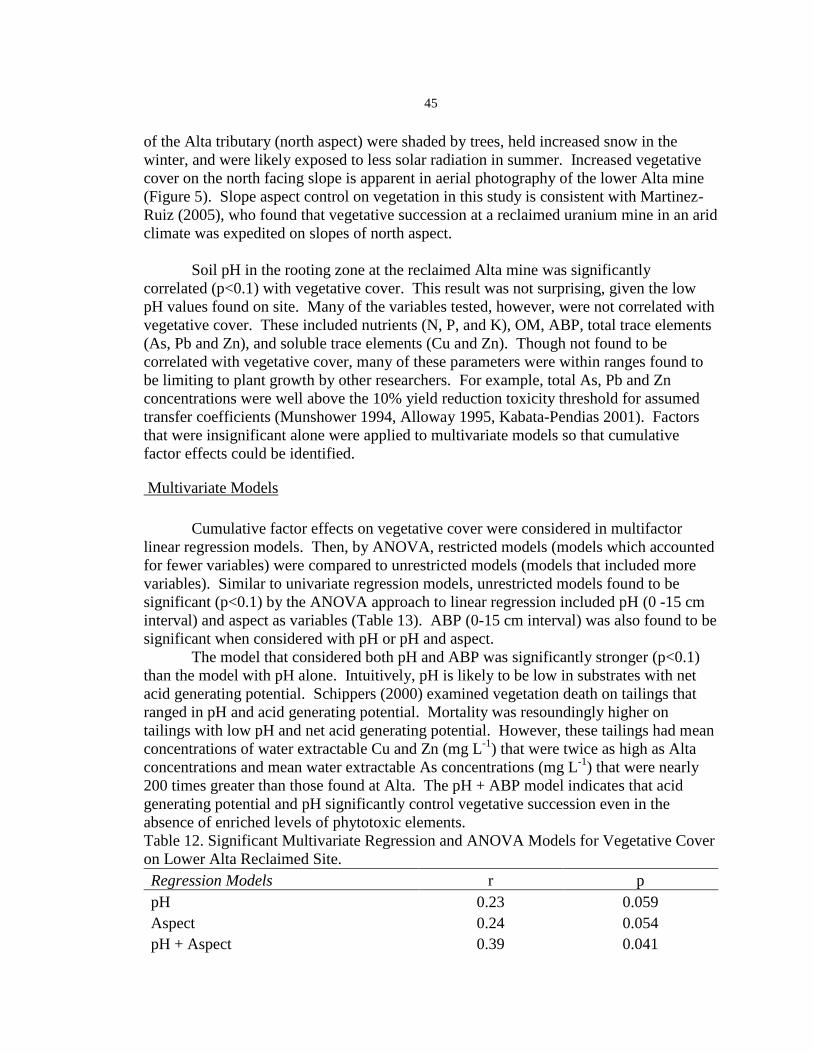
45
of the Alta tributary (north aspect) were shaded by trees, held increased snow in the
winter, and were likely exposed to less solar radiation in summer. Increased vegetative
cover on the north facing slope is apparent in aerial photography of the lower Alta mine
(Figure 5). Slope aspect control on vegetation in this study is consistent with Martinez-
Ruiz (2005), who found that vegetative succession at a reclaimed uranium mine in an arid
climate was expedited on slopes of north aspect.
Soil pH in the rooting zone at the reclaimed Alta mine was significantly
correlated (p<0.1) with vegetative cover. This result was not surprising, given the low
pH values found on site. Many of the variables tested, however, were not correlated with
vegetative cover. These included nutrients (N, P, and K), OM, ABP, total trace elements
(As, Pb and Zn), and soluble trace elements (Cu and Zn). Though not found to be
correlated with vegetative cover, many of these parameters were within ranges found to
be limiting to plant growth by other researchers. For example, total As, Pb and Zn
concentrations were well above the 10% yield reduction toxicity threshold for assumed
transfer coefficients (Munshower 1994, Alloway 1995, Kabata-Pendias 2001). Factors
that were insignificant alone were applied to multivariate models so that cumulative
factor effects could be identified.
Multivariate Models
Cumulative factor effects on vegetative cover were considered in multifactor
linear regression models. Then, by ANOVA, restricted models (models which accounted
for fewer variables) were compared to unrestricted models (models that included more
variables). Similar to univariate regression models, unrestricted models found to be
significant (p<0.1) by the ANOVA approach to linear regression included pH (0 -15 cm
interval) and aspect as variables (Table 13). ABP (0-15 cm interval) was also found to be
significant when considered with pH or pH and aspect.
The model that considered both pH and ABP was significantly stronger (p<0.1)
than the model with pH alone. Intuitively, pH is likely to be low in substrates with net
acid generating potential. Schippers (2000) examined vegetation death on tailings that
ranged in pH and acid generating potential. Mortality was resoundingly higher on
tailings with low pH and net acid generating potential. However, these tailings had mean
concentrations of water extractable Cu and Zn (mg L-1
) that were twice as high as Alta
concentrations and mean water extractable As concentrations (mg L-1
) that were nearly
200 times greater than those found at Alta. The pH + ABP model indicates that acid
generating potential and pH significantly control vegetative succession even in the
absence of enriched levels of phytotoxic elements.
Table 12. Significant Multivariate Regression and ANOVA Models for Vegetative Cover
on Lower Alta Reclaimed Site.
Regression Models r p
pH 0.23 0.059
Aspect 0.24 0.054
pH + Aspect 0.39 0.041
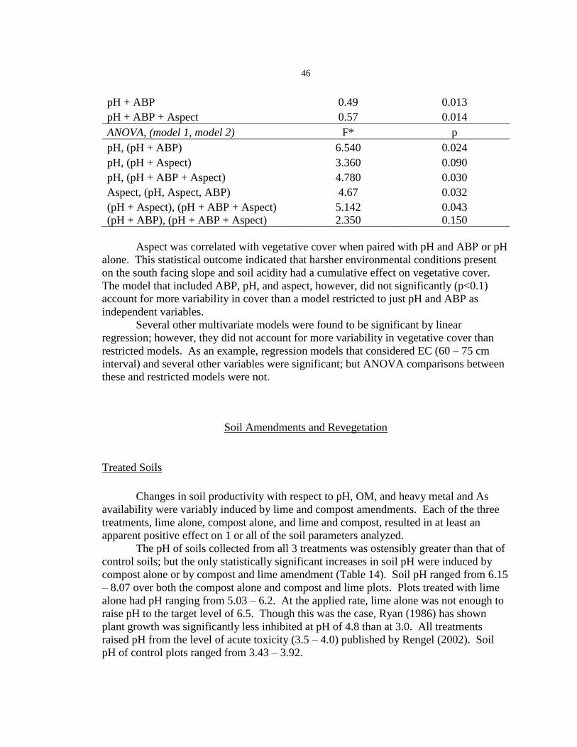
46
pH + ABP 0.49 0.013
pH + ABP + Aspect 0.57 0.014
ANOVA, (model 1, model 2) F* p
pH, (pH + ABP) 6.540 0.024
pH, (pH + Aspect) 3.360 0.090
pH, (pH + ABP + Aspect) 4.780 0.030
Aspect, (pH, Aspect, ABP) 4.67 0.032
(pH + Aspect), (pH + ABP + Aspect) 5.142 0.043
(pH + ABP), (pH + ABP + Aspect) 2.350 0.150
Aspect was correlated with vegetative cover when paired with pH and ABP or pH
alone. This statistical outcome indicated that harsher environmental conditions present
on the south facing slope and soil acidity had a cumulative effect on vegetative cover.
The model that included ABP, pH, and aspect, however, did not significantly (p<0.1)
account for more variability in cover than a model restricted to just pH and ABP as
independent variables.
Several other multivariate models were found to be significant by linear
regression; however, they did not account for more variability in vegetative cover than
restricted models. As an example, regression models that considered EC (60 – 75 cm
interval) and several other variables were significant; but ANOVA comparisons between
these and restricted models were not.
Soil Amendments and Revegetation
Treated Soils
Changes in soil productivity with respect to pH, OM, and heavy metal and As
availability were variably induced by lime and compost amendments. Each of the three
treatments, lime alone, compost alone, and lime and compost, resulted in at least an
apparent positive effect on 1 or all of the soil parameters analyzed.
The pH of soils collected from all 3 treatments was ostensibly greater than that of
control soils; but the only statistically significant increases in soil pH were induced by
compost alone or by compost and lime amendment (Table 14). Soil pH ranged from 6.15
– 8.07 over both the compost alone and compost and lime plots. Plots treated with lime
alone had pH ranging from 5.03 – 6.2. At the applied rate, lime alone was not enough to
raise pH to the target level of 6.5. Though this was the case, Ryan (1986) has shown
plant growth was significantly less inhibited at pH of 4.8 than at 3.0. All treatments
raised pH from the level of acute toxicity (3.5 – 4.0) published by Rengel (2002). Soil
pH of control plots ranged from 3.43 – 3.92.

47
All plots that received compost were within the targeted range of 2 – 6% OM at
the end of the growing season. Control and lime plots, which received no compost, were
below or at the lower end of the targeted range. Soil OM for these plots ranged from 1.8
– 3.0%. The resulting increase in OM was significant for compost and lime treatments
but not for the compost alone treatment; although OM in soils of the compost treatment
was noticeably higher than non-compost plots (Table 14).
Table 13. Soil pH and OM in Treated Soils
Soil pH and OM expressed as mean of 4 replicates
No. of
treatments pH
OM
Treatment (%)
Control 4 3.68 b 2.15 b
Lime 4 5.73 b 2.38 b
Compost 4 7.08 a 4.28 a,b
Compost & Lime 4 7.27 a 5.1 a
Values followed by same letter within columns are not significantly different (p<0.1).
Water extractable metal levels in soils of both the compost and lime and compost
plots were not detectable by 10:1 extraction and ICPMS (Table 15). Pb was not
detectable for all soils tested. Zn in the control soil and lime amended soils appeared
higher than Zn in compost and lime and composted soils; but significant statistical
differences were not found due to non detected (ND) values. Lime treatment resulted in a
significant (p<0.1) difference in extractable As concentration. Relatively low values of
each element were likely not significant inhibitors to plant growth.
Table 14. Water Extractable As and Heavy Metals (mg kg-1
) in Treated Soils.
Extractable Heavy Metals and As
Treatment As Cd Cu Pb Zn
Control 0.22 ± 0.29 a ND - 2.0 13 ± 12.7 ND 84.25 ± 77.3
Lime 0.035 ± 0.01 b ND - 1.0 ND - 12 ND 38 ± 65.8
Compost 0.74 ± 0.72 a ND ND ND ND
Compost &
Lime 0.32 ± 0.037 a ND ND ND ND
Values followed by same letter within columns are not significantly different.(p<0.1)
Vegetative Cover
Despite apparent and statistically significant improvements in the relative soil
productivity of treated soils, canopy cover estimates performed at the end of the growing
season indicated that none of the treatments resulted in vegetation establishment
indicative of rehabilitated lands. Mean canopy cover was 1.48%, 3.38%, 5.53%, and
8.65% on control, lime, compost, and lime and compost treatments, correspondingly.
Neuman (2005) achieved a median canopy cover of 62.5% on plots treated with lime and
compost; and Tafi (2006) classified cover less than 25% as poor in her assessment of 3
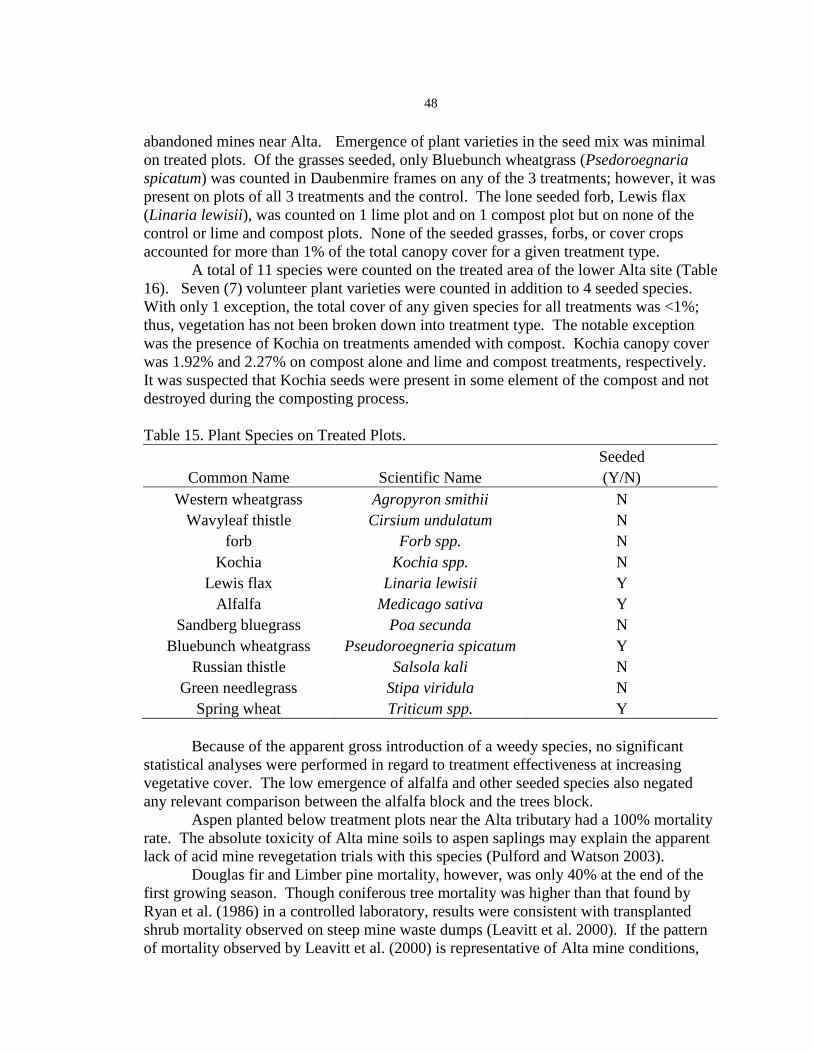
48
abandoned mines near Alta. Emergence of plant varieties in the seed mix was minimal
on treated plots. Of the grasses seeded, only Bluebunch wheatgrass (Psedoroegnaria
spicatum) was counted in Daubenmire frames on any of the 3 treatments; however, it was
present on plots of all 3 treatments and the control. The lone seeded forb, Lewis flax
(Linaria lewisii), was counted on 1 lime plot and on 1 compost plot but on none of the
control or lime and compost plots. None of the seeded grasses, forbs, or cover crops
accounted for more than 1% of the total canopy cover for a given treatment type.
A total of 11 species were counted on the treated area of the lower Alta site (Table
16). Seven (7) volunteer plant varieties were counted in addition to 4 seeded species.
With only 1 exception, the total cover of any given species for all treatments was <1%;
thus, vegetation has not been broken down into treatment type. The notable exception
was the presence of Kochia on treatments amended with compost. Kochia canopy cover
was 1.92% and 2.27% on compost alone and lime and compost treatments, respectively.
It was suspected that Kochia seeds were present in some element of the compost and not
destroyed during the composting process.
Table 15. Plant Species on Treated Plots.
Seeded
Common Name Scientific Name (Y/N)
Western wheatgrass Agropyron smithii N
Wavyleaf thistle Cirsium undulatum N
forb Forb spp. N
Kochia Kochia spp. N
Lewis flax Linaria lewisii Y
Alfalfa Medicago sativa Y
Sandberg bluegrass Poa secunda N
Bluebunch wheatgrass Pseudoroegneria spicatum Y
Russian thistle Salsola kali N
Green needlegrass Stipa viridula N
Spring wheat Triticum spp. Y
Because of the apparent gross introduction of a weedy species, no significant
statistical analyses were performed in regard to treatment effectiveness at increasing
vegetative cover. The low emergence of alfalfa and other seeded species also negated
any relevant comparison between the alfalfa block and the trees block.
Aspen planted below treatment plots near the Alta tributary had a 100% mortality
rate. The absolute toxicity of Alta mine soils to aspen saplings may explain the apparent
lack of acid mine revegetation trials with this species (Pulford and Watson 2003).
Douglas fir and Limber pine mortality, however, was only 40% at the end of the
first growing season. Though coniferous tree mortality was higher than that found by
Ryan et al. (1986) in a controlled laboratory, results were consistent with transplanted
shrub mortality observed on steep mine waste dumps (Leavitt et al. 2000). If the pattern
of mortality observed by Leavitt et al. (2000) is representative of Alta mine conditions,
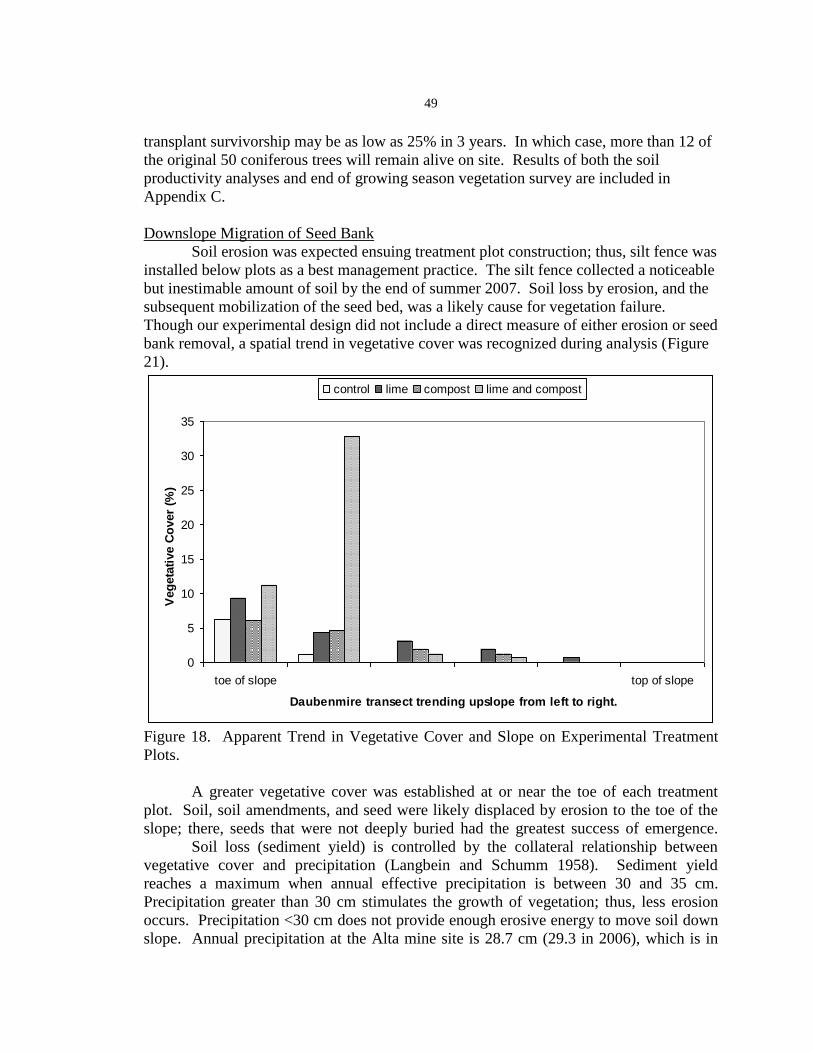
49
transplant survivorship may be as low as 25% in 3 years. In which case, more than 12 of
the original 50 coniferous trees will remain alive on site. Results of both the soil
productivity analyses and end of growing season vegetation survey are included in
Appendix C.
Downslope Migration of Seed Bank
Soil erosion was expected ensuing treatment plot construction; thus, silt fence was
installed below plots as a best management practice. The silt fence collected a noticeable
but inestimable amount of soil by the end of summer 2007. Soil loss by erosion, and the
subsequent mobilization of the seed bed, was a likely cause for vegetation failure.
Though our experimental design did not include a direct measure of either erosion or seed
bank removal, a spatial trend in vegetative cover was recognized during analysis (Figure
21).
0
5
10
15
20
25
30
35
toe of slope top of slope
Daubenmire transect trending upslope from left to right.
Veg
eta
tive C
over
(%)
control lime compost lime and compost
Figure 18. Apparent Trend in Vegetative Cover and Slope on Experimental Treatment
Plots.
A greater vegetative cover was established at or near the toe of each treatment
plot. Soil, soil amendments, and seed were likely displaced by erosion to the toe of the
slope; there, seeds that were not deeply buried had the greatest success of emergence.
Soil loss (sediment yield) is controlled by the collateral relationship between
vegetative cover and precipitation (Langbein and Schumm 1958). Sediment yield
reaches a maximum when annual effective precipitation is between 30 and 35 cm.
Precipitation greater than 30 cm stimulates the growth of vegetation; thus, less erosion
occurs. Precipitation <30 cm does not provide enough erosive energy to move soil down
slope. Annual precipitation at the Alta mine site is 28.7 cm (29.3 in 2006), which is in

50
the range that limits vegetation and practically in the range suggested to yield increased
erosion. In unamended soils, the amount of soil loss is compounded by other controlling
variables like acidity, which has already been shown to effect plant growth.

51
CONCLUSIONS AND RECOMMENDATIONS
Three (3) hypotheses were tested in 2 years (2006 – 2007) of study at the
abandoned reclaimed Alta mine complex: 1) Waters that drain the site are the significant
source of impairment to downstream water quality in terms of total maximum As, Cd,
Cu, Pb, Zn, and sediment load; 2) Alta mine soils are still impacted by chemical or
physical influences that preclude vegetative cover; and 3) Lime and compost
amendments applied to experimental plots would improve soil productivity and
vegetative cover. Each hypothesis was accepted or rejected based on results of field
measurements and monitoring activities, laboratory analyses, and statistical inference.
Water Quality
Results of the 2006 – 2007 monitoring effort indicate that abandoned
underground mine workings, shallow subsurface flow, and soil leachate were all sources
of As and heavy metals in the Alta tributary. The Alta mine sub-watershed is not unlike
numerous other mined watersheds that have been found to discharge As and heavy metals
from various sources and media (Brooks et al. 2001, Sullivan et al. 2001, Kimball et al.
2002). The primary source of individual elements varied; but the source with the highest
overall discharge of As and heavy metals was the 180-m deep #8 shaft. The significant
contribution of AMD discharge from point source abandoned mine features such as adits,
shafts, and portals has been resoundingly confirmed by other researchers (Runkel and
Kimball 2002, Kimball et al. 2002, Caruso 2003, and Herr et al. 2003).
Patterns of As and heavy metal discharge along the longitudinal profile of the
Alta tributary downstream from the #8 shaft revealed that the Alta sub-watershed stores a
portion of the As and heavy metals loads; and solutes that do reach Corbin Creek likely
undergo chemical transformation and attenuate in the mixing zone. Decreases of metal
and As load are common in mixing zones with neutral streams (Runkel and Kimball
2002, Butler II 2006). Nonetheless, loads that remain mobile in Corbin Creek are
attributable to significant water quality impairment and hindrance to TMDL attainment.
During periods of low flow, the Alta tributary is the only source of heavy metals and As
in Corbin Creek. It was observed that flow above the Alta tributary had stopped by June
9, 2007. During flow regimes where background loads are contributed from Corbin
Creek above the Alta tributary, they equal less than 40% of the total load in Corbin Creek
below the confluence. In contrast, Alta tributary loads ranged from 286% to 1,492% of
the total As, Cd, Cu, Pb, and Zn in Corbin Creek. These results support the hypothesis
that the Alta tributary is the major source of As, Cd, Cu, Pb, and Zn in Corbin Creek.
Significantly lower loads in Corbin Creek above the Alta tributary suggest that
reclamation activities performed in the Corbin Creek watershed, namely the removal of
the Bertha tailings pile, were effective at mitigating water quality impairments. The pH
of Corbin Creek above the Alta tributary was neutral, as compared to Alta tributary pH
that ranged from 2.06 to 4.63. Removal of the Bertha tailings pile had positive effects on

52
water quality because no additional source of AMD, like the #8 shaft, was present.
However, AMD products were not the only indices of impaired water quality in the Alta
tributary.
The abundance of bare ground and uncovered waste rock still present in the Alta
sub-watershed has the potential to cause water quality impacts due to sedimentation.
Sediment accumulation in both the Alta tributary and Corbin Creek channels was evident
during the course of the study. It is likely that the sediment is carried by debris flows
during low frequency, high intensity rainfall events. These events were not monitored
during the summer of 2007; thus, further sediment samples taken during thundershowers,
such as those measured by our rain gage in August 2007, are needed to accurately
quantify the Alta tributary sediment load. For this reason, the hypothesis that the Alta
tributary is the major source of sediment in Corbin Creek could neither be accepted nor
rejected. Ideally, however, sediment load reductions could be achieved by revegetation.
Limitations on Revegetation
The physical character of soils at the reclaimed Alta mine was consistent with
soils found naturally around the Boulder Batholith (Deckler 1982, and Veseth and
Montagne 1980); however, the chemical characteristics, in terms of elevated heavy
metals, ABP, and low pH, were consistent with mine waste rock (Pioneer 1994). Acid
base accounting performed on Alta soils proved that much of the substrate was
moderately to highly net acid generating in 2006, seven years after the 1999 reclamation
effort. Soil pH was also indicative of acidic conditions. Vegetative cover was
significantly (p<0.1) controlled by net acid generating potential and low pH in soils.
Cover was also significantly (p< 0.1) influenced by slope aspect. Dry conditions
compounded acid toxicity, especially on the south facing slope. The south facing slope at
the reclaimed Alta mine was generally devoid of vegetation and had numerous eroding
rills. The hypothesis that chemical (soil pH and ABP) and physical (aspect) variables
precluded vegetation on the reclaimed Alta mine site was accepted based on statistical
significance determined by the ANOVA approach to linear regression. Other suspected
variables (i.e. heavy metals and As) were not found to significantly impact vegetative
cover.
Lime and compost amendments used to increase soil productivity on treated plots
on the south facing slope of the Alta mine had marginal success. Lime treatment alone
did not significantly (p<0.1) raise soil pH above control levels or, to the target of 6.5.
Compost alone and compost and lime treatments both resulted in soil pH that was
significantly (p<0.1) better than controls. OM content was also significantly (p<0.1)
greater in compost treated plots, with or without lime, than in control plots. Despite
increased soil productivity, none of the treated plots resulted in vegetative cover that was
indicative of successful land rehabilitation. The hypothesis that lime and compost
amendments would raise both soil productivity and vegetative cover was only partially
accepted. Lime and compost improved soil quality; but vegetation establishment at the
Alta mine was still limited.

53
The precipitation regime in southwest Montana is consistent with a level of
effective annual precipitation that does not support enough vegetation to overcome the
erosion that it creates. Sandy soils on steep south facing slopes were particularly
susceptible to erosion at the Alta mine; thus, experimental plots built during the current
revegetation effort, on the approximate original hill contour, were subject to seed loss.
Seed loss due to unstable topsoil has been the unfortunate outcome of previous attempts
to revegetate steep slopes (Leavitt 2000). Slopes at the Alta site must be significantly
stabilized, by means other than terraces, before vegetation can be established. It cannot
be assumed that a vegetative cover alone will stabilize the slopes.
Bluebunch wheatgrass (Psedoroegnaria spicatum) was the lone seeded grass
species that had any apparent success during the revegetation trial. It appeared in all of
the treatment plots and on the unamended controls. Aspen (Populus tremuloides)
establishment was entirely unsuccessful in the acidic soils of the Alta mine, despite the
tree’s presence nearby. Douglas fir (Pseutosuga menziesii) and limber pine (Pinus
flexilis) exhibited some tolerance to acidic conditions, as predicated by Ryan (1986); but
40% mortality of conifers still occurred.
Abandoned Mines and Watershed Restoration
This study successfully linked abandoned, acid-producing, heavy metal mines to
major downstream water quality impairments. The Alta mine, specifically, is the major
contributing source of contaminants in Corbin Creek. Other mines of similar size, which
are abundant in southwest Montana, may need to be considered for their impact on
surface water quality and TMDL attainment status. Ineffective land rehabilitation may
have a substantial impact on water quality impairments through sediment or As and
heavy metals leached from soils. This may be true of Cu at the Alta mine, since soil-
water extractable concentrations were higher than concentrations in #8 shaft discharge.
However, deep underground mine workings were the most abundant source of other
heavy metals and As discharge at the study site. Consequently, any level of successful
land treatment will have little effect on Corbin Creek heavy metal and As TMDL
attainment status.
Recommendations
Sufficient amounts of waste rock were removed by MT DEQ in 1999 in order to
obtain surface soils at the Alta mine with As and Pb concentrations below a recreational
risk-based standard. These standards appeared to have been met; however, minimal top
soil and fertilizer application did not prevent acid generating substrates from inhibiting
plant growth. It is recommended that more emphasis be placed on soil productivity than
on arbitrary or risk-based soil metal action levels if successful revegetation is an expected
outcome of further reclamation activities at the Alta Mine. In this study, soil productivity
was increased on the south-facing slopes of the Alta reclaimed area with modest amounts
of lime and compost; yet vegetation failure resulted because of unstable slopes. It is

54
recommended that the slopes be stabilized with tackifier or erosion control fabric in
addition to soil amendment. .
It is not expected that more waste will be removed from the Alta sub-watershed;
however, residential real-estate development in the immediate vicinity may provide the
impetus for aesthetic enhancement of the landscape. In the event of further waste
removal, it is recommended that the effort be focused on sediment accumulation in the
Alta tributary channel. This research has shown the channel to be a sink for As and
heavy metals that are suspected to have coprecipitated with Fe-hydroxides in the stream
bed. The stored sediment and heavy metals have the potential to result in downstream
exceedances of aquatic life standards, TMDLs, and other water quality standards if they
are flushed during high magnitude storm events.
It is entirely meaningless to remove the heavy metal and As laden sediment if the
source of heavy metals and As is not addressed. This research identified the #8 shaft as
the most significant source of heavy metals and As in the Alta tributary; thus, the most
progressive action that could be taken at the Alta mine would be the direct treatment of
AMD discharged from the shaft. It was beyond the scope of this research to address
feasible treatment options for shaft discharge. Further research is needed to identify
applicable and cost effective water treatment options.
55
REFERENCES CITED
Abedin, M.J. Meharg, A.A. 2002. Relative toxicity of arsenite and arsenate on
germination and early seedling growth of rice (Oryza sativa L.). Plant and Soil.
243:57 – 66.
Adu-Wusu, C. Yanful, E.K. 2006. Performance of engineered test covers on acid-
generating waste rock at Whistle mine, Ontario. Canadian Geotechnical Journal. 43:1
– 18.
Alloway, B.J. 1995. The origin of heavy metals in soils. In Heavy Metals in Soils2nd
edition [Alloway, B.J. editor]. Glasgow, UK. Blackie academic and professional. 368
p.
American Public Health Association (APHA). 2001. Standard methods for the
examination of water and wastewater: including bottom sediment.
American Society of Agronomy, Inc., Soil Science Society of America, Inc. (ASA,
SSSA). 1982. Methods of soil analysis part 2-chemical and microbiological
properties, 2nd
edition. Madison, WI.
Baker, A.J.M. 1987. Metal Tolerance. New Phytologist. 106:93 – 111.
Ballen, K.G. Graham, P.H. 2002. Regulation of microbial processes by soil pH. In
Handbook of plant growth: pH the master variable [Rengel, Z. editor]. New York,
NY. Marcel Dekker, Inc. 446 p.
Basta, N.T. Ryan, J.A. Chaney, R.L. 2005. Trace element chemistry in residual-treated
soils: key concepts and metal bioavailability. Journal of Environmental Quality.
34:49- 63.
Becraft, G.E. Pinckney, D.M. Rosenblum, S. 1963. Geology and mineral deposits of the
Jefferson City quadrangle, Jefferson and Lewis and Clark Counties, Montana. USGS
Professional Paper 428.
Benda, L. 1990. Influence of debris flows on channels and valley floors in the Oregon
Coast Range, U.S.A. Earth Surface Processes and Landforms. 15(5):457 – 466.
Bonta, J.V. 2000. Impact of coal surface mining and reclamation on suspended sediment
in three Ohio watersheds. Journal of the American Water Resources Association.
36(4):869 – 887.
56
Borgegard, S.O. Rydin, H. 1989. Biomass, root penetration and heavy metal uptake in
birch in a soil cover over copper tailings. The Journal of Applied Ecology. 26: 585 -
595.
Brooks, P.D. McKnight, D.M. Bencala, K.E. 2001. Annual maxima in Zn concentrations
during spring snowmelt in streams impacted by mine drainage. Environmental
Geology. 40:1447 – 1454.
Broshears, R.E. 1996. Reactive solute transport in acidic streams. Water, Air and Soil
Pollution. 90:195 – 204.
Butler II, T.W. 2006. Geochemical and biological controls on trace metal transport.
Environmental Geochemistry and Health. 28:231 – 241.
Cardon, G.E. Davis, J.G. Bauder, T.A. Waskom, R.M. 2003. Salt-affected soils. Colorado
State University Extension Publication no. 0.503.
Caruso, B.S. 2003. Water quality simulation for planning restoration of mined
watersheds. Water, Air, and Soil Pollution. 150:359 -382.
Cela, S. Sumner, M.E. 2002a. Critical concentrations of copper, nickel, lead, and
cadmium in soils based on nitrification. Communications in Soil Science and Plant
Analysis. 33(1):19 – 30.
Cela, S. Sumner, M.E. 2002b. Soil zinc fractions determine inhibition of nitrification.
Water, Air, and Soil Pollution. 141:91 - 104.
Christensen, T.H. 1984. Cadmium soil sorption at low concentrations: I. effect of time,
cadmium load, pH, and calcium. Water, Air, and Soil Pollution. 21:105 – 114.
Colbeck, S., Akitaya, E., Armstrong, R., Gubler, H., Lafeuille, J, Lied, K., McClung, D.,
Morris, E. 1990. The international classification for seasonal snow on the ground:
International Association of Scientific Hydrology. 23 p.
Crowley, D.E. Alvey, S.A. 2002. Regulation of microbial processes by soil pH. In
Handbook of plant growth: pH the master variable [Rengel, Z. editor]. New York,
NY. Marcel Dekker, Inc. 446 p.
Datta, R. Sarkar, D. 2004. Effective integration of soil chemistry and plant molecular
biology in phytoremediation of metals: an overview. Environmental Geosciences. 11:
53 – 63.
Daubenmire, R. 1959. A canopy coverage method of vegetational analysis. Northwest
Science. 33:43-64.

57
Deckler, J.H. 1982. Characterization of four inactive hard rock mines in western
Montana. M.S. thesis, Land Rehabilitation. Montana State University. Bozeman, MT.
Devore, J. Farnum, N. 2005. Applied statistics for engineers and scientists 2nd
edition.
Belmont, CA: Thomson Brooks/Cole. 605p.
Edwards, T.K. Glysson, D.G. 1999. Field Methods for Measurement of fluvial sediment.
U.S. Geological Survey Techniques of Water Resources Investigations, Book 3,
Chapter C2.
Evangelou, V.P. 1995. Pyrite oxidation and its control. Boca Raton, FL: CRC Press. 293
p.
Foth, H.D. Ellis, B.G. 1997. Soil Fertility 2nd
Edition. Boca Raton, FL: CRC Press. 290 p.
Friesl, W. Lombi, E. Horak, O. Wenzel, W.W. 2003. Immobilization of heavy metals in
soils using inorganic amendments in a greenhouse study. Journal of Plant Nutrition
Soil Science. 166:191 – 196.
Gallagher, L.M. 2001. Clean water act. In Enivironmental law handbook [Sullivan T.F.P.
editor]. Rockville, MD. Government Institutes,Inc. 811p.
Gilbert, G.K. 1917. Hydraulic mining debris in the Sierra Nevada. USGS Professional
Paper 105. Wasington D.C. Government Printing Office. 154 p.
Goldberg, S. 2002. Competitive adsorption of arsenate and arsenite on oxides and clay
minerals. Soil Science Society of America Journal. 66:413 – 421.
Henry, T.B. Irwin, E.R. Grizzle, J.M. Wildhaber, M.L. Brunbaugh, W.G. 1999. Acute
toxicity of an acid mine drainage mixing zone to juvenile bluegill and largemouth
bass. Transactions of the American Fisheries Society. 128: 919-928.
Herr, J.W. Chen, C.W. Goldstein, R.A. Herd, R. Brown, M.J. 2003. Modeling acid mine
drainage on a watershed scale for TMDL calculations. Journal of the American Water
Resources Association. 39(2):289 – 300.
Inskeep, W.P. McDermott, T.R. Fendorf, S. 2002. Arsenic cycling in soils and natural
waters: chemical and microbiological processes. In Environmental Chemistry of
Arsenic [Frankenberger Jr., W.T. editor]. New York, NY. Marcel Dekker, Inc. 391p.
Jain, A. Raven, K.P. Loeppert, R.H. 1999. Arsenite and arsenate adsorption on
ferrihydrite: surface charge reduction and net OH- release stoichiometry.
Environmental Science and Technology. 33(8):1179 – 1184.

58
Jain, A. Loeppert, R.H. 2000. Effect of competing anions on the adsorption of arsenate
and arsenite by ferrihydrite. Journal of Environmental Quality. 29:1422 – 1430.
Jennings, S.R., Dollhopf, D.J. 1995. Geochemical characterization of sulfide mineral
weathering for remediation of acid producing mine wastes. Reclamation Research
Unit, Montana State University, Bozeman, MT. Reclamation Research Publ. No.
9502.
Jiang, Q.Q. Singh, B.R. 2004. Effect of different forms and sources of arsenic on crop
yield and arsenic concentration. Water, Air, and Soil Pollution. 74 (3-4):321 – 343.
Jones, C.A. Inskeep, W.P. Neuman, D.R. 1997. Arsenic transport in contaminated
tailings following liming. Journal of Environmental Quality. 26: 433 – 439.
Kabata-Pendias, A. 2001. Trace elements in soils and plants 3rd
edition. Boca Raton,FL:
CRC Press. 413p.
Khan, D.H. Frankland, B. 1983. Plant and Soil. Effects of cadmium and lead on radish
plants with particular reference to movement of metals through soil profile and plant.
Plant and Soil. 70:335 – 345.
Kimball, B.A. Runkel, R.L. Walton-Day, K. Bencala, K.E. 2002. Assessment of metal
loads in watersheds affected by acid mine drainage by using tracer injection and
synoptic sampling: Cement Creek, Colorado, USA. Applied Geochemistry. 17:1183 –
1207.
Kramer, P.A. Zabowski, D. Scherer, G. Everett, G.L. 2000. Native plant restoration of
copper mine tailings: I. substrate effect on growth and nutritional status in a
greenhouse study. Journal of Environmental Quality. 29:1762 – 1769.
Langbein, W.B. Schumm, S.A. 1958. Yield of sediment in relation to mean annual
precipitation. Transactions of the American Geophysical Union.
Leavitt, K.J. Fernandez, G.C.J. Nowak, R.S. 2000. Plant establishment on angle of repose
mine waste dumps. Journal of Range Management. 53:442 – 452.
Lefebvre, R. Hockley, D. Smolensky, J. Gelinas, P. 2001. Multiphase transfer processes
in waste rock piles producing acid mine drainage 1: conceptual model and system
characteristics. Journal of Contaminant Hydrology. 52:1-4, 137 – 164.
Ma, L.Q. Rao, G.N. 1997. Chemical fractionation of cadmium, copper, nickel, and zinc
in contaminated soils. Journal of Environmental Quality. 26:259 – 264.

59
Macdonald, B. 1986. Practical woody plant propagation for nursery growers. Portland,
OR. Timber Press. 669p.
Macdonald, B.C.T. White, I. Astrom, M.E. Keene, A.F. Melville, M.D. Reynolds, J.K.
2007. Discharge of weathering products from acid sulfate soils after a rainfall event,
Tweed River, eastern Australia. Applied Geochemistry. 22: 2695 – 2705,
Manning, B.A. Goldberg, S. 1997. Arsenic(III) and arsenic(V) adsorption on three
California soils. Soil Science. 162(12):886 – 895.
Manning, B.A. Suarez, D.L. 2000. Modeling arsenic(III) adsorption and heterogenous
oxidation kinetics in soils. Soil Science Society of America Journal. 64:128 – 137.
Marin, A.R. Masscheyleyn, P.H. Patrick Jr., W.H. 1993. Soil redox-pH stability of
arsenic species and its uptake on arsenic uptake by rice. Plant and Soil. 152(2):245 -
253
Martinez, C.E. Motto, H.L. 2000. Solubility of lead, zinc, and copper added to mineral
soils. Environmental Pollution. 107: 153 – 158.
Marcus, A.W. Meyer, G.A. Nimmo, D.R. 2001. Geomorphic control of persistent mine
impacts in a Yellowstone Park stream and implications for the recovery of a fluvial
system. Geology. 29(4):355- 358.
Montana Department of Environmental Quality (MT DEQ). 2005. A guide to abandoned
mine reclamation. Published online at:
http://www.deq.state.mt.us/abandonedmines/bluebook.asp. Accessed January 2008.
Montana Department of Environmental Quality (MT DEQ). 2006. Montana numeric
water quality standards. Circular DEQ-7. Helena, MT. 40p.
Montana Department of Environmental Quality (MT DEQ). 2008. Priority mine sites.
Published online at: http://www.deq.state.mt.us/abandonedmines/priority.asp.
Accessed January 2008.
Nelson, D.W. Sommers, L.E. 1996. Total carbon, organic carbon, and organic matter. In
Methods of soil analysis part 3 – chemical methods [Sparks, D.L. editor]. Madison,
WI. Soil Science Society of America. 1390p.
Neuman, D. R. Vandeberg, G.S. Blicker, P.B. Jennings, S.R., Ford, K. 2005.
Phytostabilization of acid metalliferous mine tailings at the Keating sing in Montana.
Presented at the National Meeting of the American Society of Mining and
Reclamation. ASMR.

60
Niyogi, D.K. Lewis, Jr., W.M. McKnight, D.M. 2001. Litter breakdown in mountain
streams affected by mine drainage: biotic mediation of abiotic controls. Ecological
Applications. 11: 506 – 516.
Niyogi, D.K. Lewis, Jr., W.M. McKnight, D.M. 2002. Effects of stress from mine
drainage on diversity, biomass, and function of primary producers in mountain
streams. Ecosystems. 5:554 – 567.
O’Dell, R. Silk, W. Green, P. Claassen, V. 2007. Compost amendment of Cu-Zn
minespoil reduces toxic bioavailable heavy metal concentrations and promotes
establishment and biomass production of Bromus carinatus (Hook and Arn.).
Environmental Pollution. 148:115 – 124.
Ohio State University Research Foundation. 1971. Acid mine drainage formation and
abatement. EPA 14010 FPR 04/71.
O’Neill, P. 1995. Arsenic. In Heavy metals in soils 2nd
edition [Alloway, B.J. editor].
Glasgow, UK. Blackie academic and professional. 368 p.
Peppas, A. Komnitsas, K. Halikia, I. 2000. Use of organic covers for acid mine drainage
control. Minerals Engineering. 13:563 – 574.
Pioneer Technical Services, Inc. 1994. Abandoned hardrock mines priority sites:
summary report. Montana Department of State Lands-Abandoned Mine Reclamation
Bureau.
PRC Environmental Management, Inc. (PRC EMI). 1997. Expanded engineering
evaluation/cost analysis for the Alta Mine Jefferson County, MT. Prepared for
Montana DEQ.
Pulford, I.D. Watson, C. 2003. Phytoremediation of heavy metal-contaminated land by
trees—a review. Environmental Pollution. 29:529 – 540.
R version 2.5.1. (2007). The R foundation for statistical computing. Copyright © 2007.
Reclamation Research Unit. Bitteroot Restoration, Inc. (RRU-BRI). 2004. Clark Fork
River riparian evaluation system a remedial design tool. Prepared for US EPA,
region 8. Montana office.
Reddy, K.J. Wang, L. Gloss, S.P. 1995. Solubility and mobility of copper, zinc, and lead
in acidic environments. Plant and Soil. 171:53 – 58.
61
Rengel, Z. 2002. Role of pH in availability of ions in soil. In Handbook of plant growth:
pH the master variable [Rengel, Z. editor]. New York, NY. Marcel Dekker, Inc. 446
p.
Runkel, R.T. Kimball, B.A. 2002. Evaluating remedial alternatives for an acid drainage
stream: application of a reactive transport model. Environmental Science and
Technology. 36:1093 – 1101.
Ryan, P.J. Gessel, S.P. Zasoski, R.J. 1986. Acid tolerance of pacific northwest conifers in
solution culture. Plant and Soil. 96:239 – 257.
Schippers, A. Jozsa, P.G. Sand, W. Kovacs, Z.M. Marian, M. 2000. Microbiological
pyrite oxidation in a mine tailings heap and its relevance to the death of vegetation.
Geomicrobiology Journal. 17:2, 151 – 162.
Schroth, A.W. 2001. Geochemical pathways and processes in an acid mine drainage
system, Alta mine, MT. M.S. thesis, Geology. Northern Arizona University.
Flagstaff, AZ.
Schroth, A.W. Parnell Jr., R.A. 2005. Trace metal retention through the schwertmannite
to goethite transformation as observed in a field setting, Alta mine, MT. Applied
Geochemistry. 20:907 – 917.
Sobek, A.A. Schuller, W.A. Freeman, J.R. Smith, R.M. 1978. Field and laboratory
methods applicable to overburdens and minesoils. U.S. Environmental Protection
Agency Environmental Protection Technology. Cincinnati, OH: EPA-600/2-78-054.
Soucek, D.J. Cherry, D.S. Currie, R.J. Latimer, H.A. Trent, C.G. 2000a. Laboratory to
field validation in an integrative assessment of an acid mine drainage-impacted
watershed. Environmental Technology and Chemistry. 19: 1036 -1043.
Soucek, D.J. Cherry, D.S. Trent, C.G. 2000b. Relative acute toxicity of acid mine
drainage water column and sediments to Daphnia magna in Puckett’s Creek
watershed, Virginia, USA. Archives of Envirionmental Contamination and
Toxicology. 38: 305 – 310.
Sracek, O. Choquett, M. Gelinas, P. Lefebvre, R. Nicholson, R.V. 2004. Geochemical
characterization of acid mine drainage from a waste rock pile, Mine Doyon, Quebec,
Canada. Journal of Contaminant Hydrology. 69: 45 – 71.
Sullivan, A.B. Drever, J.I. 2001. Spatiotemporal variablilty in stream chemistry in a high-
elevation catchment affected by mine drainage. Journal of Hydrology. 252: 237 –
250.

62
Tafi, T.C. 2006. Reclamation effectiveness at three reclaimed abandoned mine sites in
Jefferson County, Montana. M.S. Thesis, Land Rehabilitation. Montana State
University. Bozeman, MT.
Tan, K.H. 2005. Soil sampling, preparation, and analysis 2nd
edition. Boca Raton, FL:
CRC Press. 623 p.
Temminghoff, E.J.M. Van Der Zee, S.E.A.T.M. De Haan, F.A.M. 1997. Copper mobility
in a copper contaminated sandy soil as affected by pH and solid and dissolved organic
matter. Environmental Science and Technology. 31:1109 – 1115.
Tetra Tech 1997. Hydrogeologic evaluation of the Alta mine site, Jefferson County, MT.
Prepared for MTDEQ.
Tetra Tech. 2002. Construction report for the Alta lower waste rock dump reclamation
project, Jefferson County, MT. Prepared for MT-DEQ.
Thomann, R.V. Mueller, J.A. 1987. Principles of surface water quality modeling and
control. New York, NY. Harper Collins Publishers. 644p.
Tordoff, G.M. Baker, A.J.M. Willis, A.J. 2000. Current approaches to the revegetation of
metalliferous mine wastes. Chemosphere. 41, 219 – 228.
U.S. Department of Agriculture, Natural Resources Conservation Service (USDA,
NRCS). 2007. National Soil Survey Handbook, title 430-VI. [Online] Available:
http://soils.usda.gov/technical/handbook/
U.S. EPA. 1995. In test methods for evaluating solid waste, 3rd
edition, 3rd
update.
Washington, D.C.
U.S. EPA. 2006. Framework water quality restoration plan and total maximum daily
loads (TMDLs) for the Lake Helena Watershed Planning Area: volume II final report.
Prepared for the MT-DEQ.
U.S. Environmental Protection Agency National Research Laboratory (US EPA, NERL).
1993. Methods for the determination of inorganic substances in environmental
samples. EPA/600/R-93/100.
Weggler-Beaton, K. McLaughlin, M.J. Graham, R.D. 2000. Salinity increases cadmium
uptake by wheat and Swiss chard from soil amended with biosolids. Australian
Journal of Soil Research. 38(1): 37 – 47.
Whitney, D.A. Lamond, R.E. 1993. Liming acid soils. Kansas State University
Agricultural Experiment Station and Cooperative Extension Service. MF-1065.

63
Wu, L. Antonovics, J. 1975. Zinc and copper uptake by Agrostis stolinifera, tolerant to
both zinc and copper. New Phytologist. 75:231 – 237.
Xian, X. 1989. Effect of chemical forms of cadmium, zinc, and lead in polluted soils on
their uptake by cabbage plants. Plant and Soil. 113: 257 – 264.
Ye, Z.H. Wong, J.W.C. Wong, M.H. 2000. Vegetation response to lime and manure
compost amendments on lead/zinc mine tailings: a greenhouse study. Restoration
Ecology. 8:3, 289 – 295.
Zhixun, L. Herbert Jr., R.B. 1996. Heavy metal retention in secondary precipitates from a
mine rock dump and underlying soil, Dalarna, Sweden. Environmental Geology. 33:1
– 12.

The Importance of Ecologically Connected Streams to theBiological Diversity of Watersheds: a case study in the St.Regis River subbasin, Montana
Basic Information
Title: The Importance of Ecologically Connected Streams to the Biological Diversity ofWatersheds: a case study in the St. Regis River subbasin, Montana
Project Number: 2008MT165BStart Date: 3/1/2008End Date: 2/28/2010
Funding Source: 104BCongressional
District: At-Large
ResearchCategory: Biological Sciences
Focus Category: Conservation, Management and Planning, EcologyDescriptors:
PrincipalInvestigators: Winsor Lowe
Publication
The Importance of Ecologically Connected Streams to the Biological Diversity of Watersheds: a case study in the St. Regis River subbasin, Montana
The Importance of Ecologically Connected Streams to the Biological Diversity of Watersheds: a case study in the St. Regis River subbasin, Montana1

The Importance of Ecologically Connected Streams to the Biological Diversity of
Watersheds: a case study in the St. Regis River subbasin, Montana
Montana Water Center USGS grant
Interim Report
by
Winsor Lowe, PhD
Assistant Professor Division of Biological Sciences
University of Montana – Missoula
Overview: For this grant, we proposed to (1) identify variables that influence patterns of
IGS distribution and abundance, (2) to use genetics (microsatellite DNA markers) and (3)
mark-capture-recapture (MCR) to assess the importance of connected stream networks to
IGS population persistence and (4) to determine the affect of human disturbance on
stream connectivity. To date, we have completed objectives 2 and 3. This summer, we
will complete our surveys in the St. Regis basin in order to identify variables associated
with IGS distribution and abundance. We will then summarize all of our data to complete
objective 4. Below, we share the results to date on objectives 1 – 3.
Objective 1: To identify variables that influence patterns of IGS distribution and
abundance
Abstract: Stream substrate disturbance is an important driver of community
composition. Substrate moves when the driving forces of water on the stream bed exceed
the resisting forces holding the substrate. Channel morphology can mitigate disturbance
be shifting the balance between driving and resisting forces. We assessed the importance
of high flow disturbance and channel morphology on the occurrence and density of a
stream salamander, Dicamptodon aterrimus (Idaho Giant salamander) in 30 streams in
the St. Regis basin of Montana. We compared support for models that describe D.
aterrimus occurrence and density as a function of channel confinement (bankfull width:
valley width) and the ratio of bankfull flow competence (τ*) to the shear stress required
to set a particle into motion (τc*). These models were compared to the top-ranked models
that described salamander occupancy and density as functions of habitat quality,
connectivity, and fragmentation in a previous study (Sepulveda and Lowe, in press). We
hypothesized that channel geomorphology influences D. aterrimus occupancy and
density during high flow and predicted that streams with low confinement and low τ*: τc*
would have greater occupancy and density. Support for channel confinement’s influence
on salamander occupancy and density was plausible, but had less support than models
from the previous study. Probability of occurrence and density increased as channel
confinement decreased, but τ*: τc* had little effect. Results suggest that salamanders are
(1) resistant to high flow disturbance and/or that (2) that disturbance has low intensity
because high flows do not mobilize the entire stream bed. Experimental studies are
needed to better understand how channel morphology and high flows interact to affect
stream organisms.

Methods: In 2006 and 2007, I surveyed 30 headwater streams in the St. Regis River
basin. Within each stream, I surveyed two 50-m reaches separated by 200 m for D.
aterrimus occurrence and density. The lower reach began 25 m upstream of the
confluence with a similar or higher-order stream. I used a backpack electrofisher to
search for salamanders within the stream. To determine detection probability, all reaches
were surveyed three times within one season. I used D. aterrimus occurrence
(presence/absence) and density within a stream as response variables. Dicamptodon
aterrimus were declared present in a headwater stream if they were detected in at least
one 50-m reach in at least one of the three surveys. I calculated density for each
headwater stream as the mean number of salamanders per m2 captured in the lower and
upper stream reaches over the three surveys.
Channel geomorphology variables: I used channel confinement and the ratio of bankfull
flow competence (τ*) to the shear stress required to set a particle into motion (τc*) as
predictor variables (Table 1). Channel confinement was calculated as the ratio of valley
width to channel width such that high values describe low confinement. Competence is a
dimension-free measure of the shear stress exerted by the flow on the bed and was
calculated as
Dg
gdS
s )(*
,
where ρs and ρ are the sediment and fluid densities, respectively; g is the acceleration of
gravity, d is maximum flow depth, and D is the median particle size (Church 2006).
Because τc* values range from 0.03 to 0.06 in most streams, I set τc* = 0.045 for all
stream reaches.
To estimate channel confinement and τ*:τc*, I measured valley width using USGS
digital elevation maps. In the field, I measured bankfull width at four random, 1-m wide
transects that extended between bank-full channel edges within each reach. At six
random points along each transect, I recorded stream depth and substrate particle
diameter. Stream slope was estimated as the difference in elevation between the upstream
and downstream ends of each plot divided by the distance between these points. Abiotic
variables were averaged across the two study reaches within each headwater stream.
Top-ranked variables: I also estimated variables associated with the top-ranked models
from Sepulveda and Lowe (in press). The top-ranked occupancy model included habitat
connectivity, fragmentation, and alteration and the top-ranked density model included the
proportion of fine and embedded substrate (Table 1). I measured habitat connectivity as
the minimum distance along the stream corridor from the mouth of the sampled
headwater drainage to the mouth of the nearest headwater drainage. I characterized
habitat fragmentation and alteration by road density and forest structure. I quantified road
density as length of roads standardized by headwater drainage area (km of road per km2)
using the 2001 Inventoried Roadless Area data layer for the Clearwater National Forest. I
described forest structure as the density of old-growth trees (trees per km2). I also
recorded the proportion of fine substrate (< 2 mm) and substrate that was embedded,
defined as having visible vertical surfaces buried in either silt or sand (Welsh et al., 1997)

at 6 points along each transect within each study reach. Proportions of embedded and fine
substrate were positively correlated, so I used principle components analysis (PCA) to
produce one axis that accounted for 75% of this variation (coefficients of the first
eigenvector: embedded substrate = 0.71, proportion of fines substrate = 0.71).
Statistical analysis and model selection: To identify predictors of D. aterrimus
occupancy, I compared two sets of models: (1) all possible combinations of the three
channel geomorphology variables and, (2) the top-ranked model from Sepulveda and
Lowe (in press), which included habitat connectivity, fragmentation, and alteration. To
identify predictors of D. aterrimus density, I compared two sets of models: (1) all
possible combinations of the three channel geomorphology variables and, (2) the top-
ranked model from Sepulveda and Lowe (in press), which included the proportion of
fine-embedded substrate. I then used model selection to identify the most plausible
statistical models for predicting D. aterrimus and probability of occurrence and density
when present. Prior to this analysis, I tested for highly correlated pairs of variables (those
with r ≥ 0.7) and used PCA to reduce collinearity among these variables. Logistic
regression was used to determine the relative likelihood of each candidate occupancy
model and multiple linear regression was used to determine the relative likelihood of
each candidate density model. Finally, I used Akaike’s Information Criterion for small
samples (AICc) based methods to select the best models of occurrence and density from
sets of candidate models (Burnham and Anderson, 2002).
I determined strength of support for the model using ΔAICc values and AICc weights
(ω). Models with ΔAICc ≤ 4 for small sample size (n/K < 40; where n = sample size and
K = number of parameters) have empirical support as being plausible (Burnham and
Anderson, 2002). To assess the importance of individual parameters within the presented
models, I calculated importance weights by summing ω values of all models in which the
parameter occurs (Burnham and Anderson, 2002). Parameters with importance weights >
0.20 are considered to be significant (Stoddard and Hayes, 2005). Finally, coefficients (β)
of local and landscape habitat covariates for D. aterrimus occurrence and relative density
where obtained by averaging across all models weighted by ω (i.e., model averaging;
Burnham and Anderson, 2002). Odds ratios were calculated from D. aterrimus
occurrence coefficient estimates as exp(β). An odds ratio of 1.0 indicates no difference
between the proportion of sample points with or without salamanders, while odds ratios
close to zero or substantially >1.0 indicates a large difference. Odds ratios less than 1.0
indicate a negative effect while ratios greater than 1.0 indicate a positive effect (Keating
and Cherry, 2004).
Obj. 2: To use genetics (microsatellite DNA markers) to assess the importance of
connected stream networks to IGS population persistence.
Abstract: The dendritic structure of stream networks provides constraints on the
movement of freshwater organisms with individual, population and community level
consequences. This consistent structural foundation provides a system in which

examination of life-history influences on population genetic structure may reveal general
insight on dispersal in stream networks. We examined the interaction of stream network
structure with life-history and dispersal on population genetic structure of the
facultatively paedomorphic Idaho Giant salamander, Dicamptodon aterrimus in stream
networks of Idaho and Montana. We tested microsatellite data for support of population
structure models by (i) examining hierarchical partitioning of genetic variation in river
networks and (ii) testing for isolation by distance (along stream corridors and overland)
to examine the importance of within-stream and overland gene flow on population
structure. Systematic and controlled sampling within stream network scales revealed that
hierarchical structure of stream networks has a strong effect on gene flow and genetic
structure of D. aterrimus. Analysis of molecular variance (AMOVA) identified
significant structure due to differences among all hierarchical levels (among sub-basin,
among networks, among streams), where the “among network” level was responsible for
the greatest structural influence. Significant isolation by distance was detected within
networks, and in-stream distance was a strong predictor of genetic distance. Genetic
differentiation among streams within networks is driven by limited migration, but
divergence among networks and among sub-basins is driven by genetic drift. These
results identify the influence of stream network structure on evolution of a freshwater
salamander, and show that large spatial scales are important and influenced by stream
network structure. High genetic divergence over small geographic distance accompanied
by drift of adjacent stream networks may have negative effects on the ability of D.
aterrimus to respond to climate change.
Methods: To examine the spatial extent of gene flow and population structure in D.
aterrimus, I collected individuals in a systematic nested hierarchical design. I sampled
individuals in 1st-order streams that were nested within networks of confluent streams
draining into a mainstem river. Stream networks were nested within sub-basins of three
major rivers: the Lochsa (four networks), St. Joe (two networks) and St. Regis (two
networks). I collected 15 D. aterrimus from three 1st-order streams within each network.
Stream networks were selected in sub-basins such that they were separated by a common
ridge running approximately perpendicular to the mainstem river. This orientation
allowed me to test for in-stream and overland gene flow within and among adjacent
networks.
In each stream, I used an LR-20 backpack electrofisher (Smith-Root Inc., Vancouver
WA) to collect salamanders from reaches beginning at least 25 m upstream of the
confluence with a higher-order stream. Survey reaches ranged from 200-391 m in length
(mean survey length± 1 SD: 220 m ± 72.7). Two streams (LWWF and LPEF; Table 1)
were sampled with three 30-m reaches separated by approximately 15 m. I clipped a
small section of tail tissue from captured salamanders and stored it in 95% ethanol. Both
juveniles and adult salamanders were sampled. Snout-vent lengths of sampled animals
ranged from 22 mm-160 mm and weights ranged from <1 g to 130 g. All sampling took
place in July – October of 2008, except for five samples from one stream that were
collected on July of 2007 (LSSP).
Microsatellite amplification and scoring: Fifteen salamanders from each stream were
genotyped at 14 microsatellite loci developed for Dicamptodon tenebrosus and D. copei

(Curtis and Taylor, 2000; Steele et al., 2008). To extract DNA, I digested tissues with
protease in a detergent based cell lysis buffer, then precipitated proteins with an
ammonium acetate solution and DNA with isopropyl alcohol. Isolated DNA was re-
suspended in 100μl TE buffer and diluted 1:10 for polymerase chain reaction (PCR)
amplification in a PTC-100 thermocycler (MJ Research Inc., Waltham, MA) with a total
volume of 10μL. Multiplex reactions followed the QIAGEN microsatellite protocol with
a single PCR touchdown profile: primer annealing started at 67°C and dropped 0.5°C for
20 cycles, followed by 25 cycles with a 57°C annealing temperature. Microsatellite
markers Dte5, D04, D24, and D18 were PCR amplified individually following QIAGEN
microsatellite protocols with separate PCR annealing temperatures. Following individual
PCRs, these markers were pooled with multiplexed markers for fragment analysis. PCR
products were visualized on an ABI3130xl Genetic Analyzer (Applied Biosystems Inc.,
Foster City, CA) in the Murdock DNA Sequencing Facility at the University of Montana,
Missoula, USA. Allele sizes were determined using the ABI GS600LIZ ladder (Applied
Biosystems Inc.) and allele sizes were called with GeneMapper version 3.7 (Applied
Biosystems Inc.).
Genetic Analyses: Using exact tests implemented in GENEPOP version 4.0 (Raymond
and Rousset, 1995), I tested for significant departures from Hardy-Weinberg proportions
and for non-random association of pairs of loci across populations (linkage
disequilibrium). Loci that deviated from HW proportions in each population were
removed from further analyses. After removal of a single locus that deviated from HW
proportions in all populations where it was not fixed for a particular allele, I calculated
genetic diversity within-streams and examined subdivision among hierarchical levels.
Intra-population genetic diversity was calculated as allelic richness (AS), the number
of alleles observed in populations (NA), and expected and observed heterozygosity (HE,
HO) of streams. I then tested for population differentiation and the extent of gene flow
with pairwise FST, a measure of genetic divergence based on the number of different
alleles calculated in Arlequin version 3.1 (Excoffier et al., 2005). The inbreeding
coefficient, FIS was calculated for every locus in each stream to detect significant
heterozygote deficit or excess in streams (GENEPOP; (Raymond and Rousset, 1995).
For a qualitative sense of genetic structure within the data set, I examined pairwise
FST s to assess levels of divergence occurring among streams within networks and sub-
basins. Furthermore, I used a hierarchical analysis of genetic variation (AMOVA
implemented in the hierfstat package in R v 2.8.1, Goudet, 2005) to partition genetic
variance within and among hierarchical scales. I first used the entire data set to assess
patterns of genetic variance throughout the entire sampling area. Specifically, I tested for
structure at four levels: among-subbasins, among networks within subbasins, among
streams within networks, and within streams. To test for influence of local genetic
structure on overall structure, I performed two additional AMOVAs, (i) within the
Lochsa sub-basin, and (ii) within and among the St. Joe and St. Regis sub-basins. The
AMOVAs generated hierarchical F-statistics (Yang, 1998) in which FSB is divergence
among sub-basins, FAN is divergence among networks within sub-basins, FAS is
divergence among streams within networks, FIS is the inbreeding coefficient within
streams, and FST is the global divergence among streams.

Genetic structure was also visually interpreted using principal components analysis
(PCA) which reduces dimensions in a multivariate dataset such that the 1st principal
component (PC1) explains as much of the variance in allele frequencies as possible
(Reich et al., 2008). To maintain quasi-independence of the data set, I removed the
highest frequency allele of each microsatellite locus and performed the PCA on
remaining allele frequencies (Leary et al., 1993). Plots of PC 1 against PC2 were
examined to assess the similarity of allele frequencies among streams within networks,
among networks within sub-basins and among sub-basins.
I used partial Bayesian individual assignment tests (Rannala and Mountain, 1997) to
assign individuals to populations based on the expected probability of multilocus
genotypes occurring in potential sources (GENECLASS2; (Piry et al., 2004). This
method can accurately identify migrants especially when genetic differention is
substantial and many loci are used (Berry et al., 2004). I used Monte Carlo resampling
for 10,000 simulations of reference populations with the same allele frequencies and
number of individuals as sampled populations (Paetkau et al., 2004). Salamanders were
excluded from their sample stream with ≥ 99% confidence of exclusion (p ≤ 0.01) and
conservatively included in another stream when p > 0.33 (Pruett et al., 2008).
Individuals excluded from their stream origin but not included in another stream were
considered potential immigrants or descendents of immigrants from populations not
sampled. I performed three assignment tests with the above standards: (i) assignment of
individuals to sub-basins, (ii) assignment of individuals to networks, and (iii) assignment
of individuals to streams.
To understand the role of gene flow by in-stream dispersal v. overland pathways, I
tested alternative hypotheses of D. aterrimus gene flow resulting in isolation by distance
(IBD). IBD is detected by testing for correlations among matrices of genetic distance
(FST) and geographic distance with Mantel tests that correct non-independence of
pairwise points (Manly, 1997). I used two measures of pairwise distance between
midpoints of survey reaches to test alternate pathways of gene flow with FSTAT version
2.9.3.2 (Goudet, 1995).
To test the hypothesis that D. aterrimus gene flow occurs primarily along stream
corridors, I estimated the correlation between FST and stream distance in each sub-basin.
Stream distance was the shortest pathway along streams connecting two points (ArcGIS
9.2, ESRI, Redlands, CA). Second, I tested the hypothesis that gene flow in D. aterrimus
occurs primarily overland by estimating the correlation between FST and surface distance
in each sub-basin. Surface distance is a straight line distance connecting two points that
corrects for changes in elevation along the path (ArcGIS 9.2, ESRI, Redlands, CA).
Sub-basins were tested separately for IBD to detect regional differences in the scale
and strength of IBD due to in-stream v. overland gene flow. Pairwise stream and surface
distances were significantly correlated (r = 0.88, p < 0.001). Therefore, the strength of
correlations of genetic distance with stream distance v. surface distance were used to
assess in-stream v. overland gene flow.
Obj. 3: To use mark-capture-recapture to assess the importance of connected stream
networks to IGS population persistence.

Abstract: Understanding how dispersal affects community dynamics and emergent
patterns of species diversity is a major goal in stream ecology because dispersal is a
phenomenon occurring in most species and because habitat fragmentation, riparian land
use, and climate change have altered dispersal rates for many freshwater organisms. We
examined the relative contributions of dispersal between stream reaches and local
ecological and evolutionary processes within stream reaches to stream salamander
persistence and coexistence with fish. Empirical data and lab experiments suggest that
salamander and fish interactions in headwater streams are unstable because fish are
predators and superior competitors of salamanders. These data are consistent with
observations across North America that salamanders are largely limited to fishless stream
reaches. However, my data show not only that salamanders persist with fish, but also that
salamanders in reaches with fish have downstream-biased dispersal. These results call
into question the mechanisms allowing for species coexistence and lead to the hypothesis:
dispersal from upper reaches offsets negative effects of fish predation and competition in
lower reaches. In this study, we used mark-recapture methods in multiple headwater
streams to test whether dispersal could foster coexistence between the stream salamander,
Dicamptodon aterrimus (the Idaho giant salamander), and salmonid fish. We estimated
net dispersal rates, apparent survival, recruitment, and realized rate of population growth
of D. aterrimus in upstream reaches without fish and downstream reaches with fish from
multiple streams. Our results suggest that dispersal did not influence population growth
rates or coexistence with fish, and that salamander dispersal between stream reaches is
not the primary mechanism for D. aterrimus × fish coexistence. Apparent survival,
recruitment, and population growth rate did not differ between reaches within a stream.
Population growth was a function of local survival and recruitment, but not of dispersal
because there was no evident difference in net emigration between upstream and
downstream reaches. We did find that D. aterrimus movement within and between stream
reaches was common. These results suggest that local processes within stream reaches,
and not spatial processes between stream reaches, promote D. aterrimus × fish
coexistence.
Methods: To sample salamanders, we used Pollock’s robust design with five primary
sampling periods in each stream (Pollock 1982). During each primary sampling period,
secondary samples occurred 24 hours apart. All unmarked salamanders were individually
marked using fluorescent elastomer (Northwest Marine Technologies, Shaw Island,
Washington, USA) and marked individuals were recorded. The longitudinal position
(distance from the confluence, m), snout-vent length (SVL, mm), and mass (mg) of all
individuals encountered were recorded. To test the retention of fluorescent elastomer, we
clipped tails of all marked salamanders and noted individuals with a clipped tail and no
elastomer mark recaptured in the subsequent secondary period (24 hours later) and
primary period (1 month later).
Movement direction.– To test if net dispersal of D. aterrimus in upstream reaches was
downstream biased and greater than net dispersal in downstream reaches with fish, we
described D. aterrimus movement across all primary sampling periods. Movement of
recaptured individuals was measured as distance along the stream (meters) from the
position of last capture. To quantity movement, we used the frequency distributions of

distances moved, assigning negative values to downstream moves and positive values to
upstream moves, to quantify movement (Skalksi and Gilliam 2000, Lowe 2003). To
determine if salamander movement distributions were consistent within each stream, we
tested for differences in the movement distribution of the two study reaches using a
Kolmogorov-Smirnov test. We assessed directional bias by testing for skewness of the
movement distribution (Zar 1984). To better understand if salamander × fish coexistence
in downstream reaches was influenced by size-biased dispersal rather than dispersal rate,
we also tested if distance moved and directional bias were linked to salamander size
using parametric (t-test) and non-parametric (Spearman Rank correlation and Mann-
Whitney) tests.
To examine if movement distance and direction bias were influenced by our
sampling protocol, seasonal flow pulses, or seasonal breeding migrations, we tested the
hypothesis that the variance of distance moved increased linearly with time, a
characteristic of movement by simple diffusion (Skellam 1951, Turchin 1998, Skalski
and Gilliam 2000, Lowe 2003). We regressed the estimated variance of distance moved
(weighted by sample size) on time (months) using the polynomial equation y = c0 + c1t +
c2t2, where y is the variance and t is time. The hypothesis predicts c0 = 0, c1 > 0, and c2 =
0. Any temporal pulses in movement caused by sampling, discharge, or behavior would
lead to non-diffusive movement.
Apparent survival, population growth rate, and recruitment.– To assess how fish affected
local population dynamics of D. aterrimus, we used the Robust design Pradel (Huggins
closed capture) model in program MARK to model variability in apparent survival (Φ)
and realized population growth rate (λ) by stream reach and time (Pollock and Otto 1983,
Pradel 1996, White and Burnham 1999). Because Pradel models assume demographic
closure and therefore cannot incorporate transitions between populations, individuals that
dispersed between reaches had two recapture histories, each specific to a reach (Lowe et
al. 2003).
The primary parameters of interest were Φ and λ, so we first evaluated models of
capture probability (p) and recapture probability (c) to avoid unnecessary bias and
imprecision in the Φ and λ estimates (Lebreton et al. 1992). We identified the best model
of p and c for each stream by pairing the global model for Φ and λ (reach x primary
sampling period x time) with all possible combinations of p ≠ c (reach x primary
sampling period x time) and p = c (reach x primary sampling period x time). We treated p
and c as nuisance variables and they were not constrained in models that compared Φ and
λ by reach and time (Barker and White 2004, Barker et al. 2005).
To test the prediction that apparent survival was lower in reaches with fish than in
fishless reaches and that realized population growth rate did not differ between reaches
with and without fish, we modeled variability in Φ and λ by stream reach (r) and primary
sampling period. Apparent survival and λ were assumed to vary across primary sampling
periods, but be constant over secondary samples. We used Program MARK to compare
the following five models
Model 1 and 2.– Apparent survival varies by reach (Φ(r)) (Model 1), and apparent
survival is constant between reaches (Φ(.)) (Model 2). Realized population growth is
constant between reaches (λ(.)).

Model 3 and 4.– Apparent survival is constant between reaches (Φ(.)). Realized
population growth rate varies by reach (λ(r)) (Model 3), and realized population growth
rate is constant between reaches (λ(.)) (Model 4).
Model 5.– For Models 1 – 4, we assumed Φ and λ varied across primary sampling
periods because of variation in stream discharge and temperature. For Model 5, we
compared the top-ranked model from Models 1 – 4 to the same model with no variation
across primary sampling periods.
Estimation of Φ and λ allowed for the estimation of recruitment (f) because
ft = λt - Φt
in the Pradel model (Franklin 2001, Williams et al. 2002), where ft is the number of new
individuals entering the population in year t + 1 per individual in the population in year t.
We ranked competing models according to how well they were supported by the
capture data using AICc, AICc weights, and evidence ratios (a multiplicative factor for the
likelihood of the best model compared to an alternative model) (Burnham and Anderson
2002). Parameter estimates were calculated using model averaging (Burnham and
Anderson 2002). Goodness-of-fit tests are not currently possible for the Robust design
Pradel model in program MARK, so we assessed the rank stability of the best-fitting
models by entering ĉ values between 1.0 and 6.0 (e.g., Lebreton et al. 1992, Cooch and
White 2001, Lowe 2003).
To assess if D. aterrimus movement was a function of D. aterrimus density, we
regressed proportion of D. aterrimus individuals that moved greater than 1 m, 5 m, and
10 m against the average density of salamanders (individuals/m2) within each stream
reach across all primary sampling sessions. To be conservative, we used multiple
movement distances (i.e., 1 m, 5 m, and 10 m) because the distance threshold that
delineates dispersal from local movement is not known for D. aterrimus. We transformed
proportional data using the arcsine square root. Estimates of salamander abundance were
taken from our most supported Robust-design Pradel models from each stream. Stream
area was based on field measurements in August 2006 and 2008.
Summary: For this grant, we proposed to identify variables that influence patterns of
IGS distribution and abundance, to use genetics (microsatellite DNA markers) and mark-
capture-recapture (MCR) to assess the importance of connected stream networks to IGS
population persistence and to determine the affect of human disturbance on stream
connectivity. This summer, we will complete our surveys in the St. Regis basin in order
to identify variables associated with IGS distribution and abundance. We have completed
work on genetics.
Modeling the Potential for Transport of ContaminatedSediment
Basic Information
Title: Modeling the Potential for Transport of ContaminatedSediment
Project Number: 2008MT166BStart Date: 3/1/2008End Date: 2/28/2009
Funding Source: 104BCongressional District: At-Large
Research Category: Climate and Hydrologic ProcessesFocus Category: Wetlands, Floods, Models
Descriptors:Principal Investigators: Joel E. Cahoon
Publication
Modeling the Potential for Transport of Contaminated Sediment
Modeling the Potential for Transport of Contaminated Sediment 1

1
Assessing the Potential for Contaminated Sediment Resuspension
from a Mine Impacted Wetland
Jessica Mason1, Joel Cahoon
2, Matthew Blank
3, Denine Schmitz
4
1Department of Civil Engineering, Montana State University
Bozeman, Montana 59717
2Department of Civil Engineering, Montana State University
Bozeman, Montana 59717
3Western Transportation Institute, Department of Civil Engineering, Montana State University
Bozeman, Montana 59717
4Department of Land Resources and Environmental Sciences, Montana State University
Bozeman, Montana 59717
ABSTRACT
Wetlands associated with Montana hard rock mines play a paradoxical role. The benefit of
attenuating flood water and sediment has led to wetlands serving as sinks for metal precipitates
and contaminated sediment. However, during high spring runoff or storm events these wetlands
may become significant sources of resuspended contaminated sediments and generate potential
impacts to downstream recipients. Using a loosely coupled hydraulic model (HEC-RAS) and a
GIS, we explored the influence of flood events of varying magnitude on stream hydraulics and
sediment mobilization across a wetland complex located in the Blackfoot River near Lincoln,
MT. Field survey data provided a topographic template for running the hydraulic model. Spatial
interpolation and geostatistical methods were used to create spatially continuous data surfaces for
model input parameters (i.e. roughness coefficient, D50), measured contaminant concentrations
(As, Cu, Zn, Cd, Pb) for the upper 2 inches of soil, model output parameters (i.e. velocity, water
depth), and critical velocity. Combining critical velocity data layers with modeled velocity and
contaminant concentration data layers allowed us to identify zones with high contaminant
concentrations and a high potential for sediment mobilization in a spatially explicit manner.
Sensitivity analysis showed the one-dimensional hydraulic model to be increasingly sensitive to
roughness coefficients with increasing discharge. Comparison of modeled stream velocity
distributions to measured velocity distributions showed deviations from observed data in shallow
near-bank and over-bank areas. Thorough investigation of differences between modeled and
measured velocity distributions at a range of flows and across several transects at a given site
will help practitioners decide whether or not this approach will be useful and provides an avenue
for future flood risk assessment. We conclude that when carefully applied, this approach may be
a valuable tool for assessing contaminated sediment mobilization risk in areas where data is
limited and/or development of more data intensive models is not feasible.

2
1.0 INTRODUCTION
1.1 EXECUTIVE SUMMARY
Hydrologic and hydraulic analyses are used by scientists and engineers for environmental
and regulatory decisions. The integration of spatial analysis and hydrological modeling by way
of geographic information systems (GIS) is becoming an integral component of flood assessment
practices. The potential environmental impacts to downstream groundwater, surface water, and
sediment quality affect human, aquatic, and riparian resources (Werner 2001). Flood risk
assessment calls for a thorough spatial evaluation of a flood event, where risk is defined as the
relationship between hazards in the area and the area’s vulnerability, and GIS provides a tool for
this type of analysis. This study models the effect of discharge events with varying return
intervals in order to assess the potential for sediment transport from a mine-impacted wetland in
the Upper Blackfoot Mining Complex (UBMC). There has been substantial work to assess and
remediate the impact of the UBMC on aquatic resources by Helena National Forest (HNF),
Montana Department of Environmental Quality (MTDEQ), and the mining company, ASARCO.
Until recently, however, the wetland complex has largely been omitted from environmental
assessments.
The benefit of attenuating flood water and sediment has led to some wetlands serving as
sinks for metal precipitates and contaminated sediment. However, during high spring runoff or
storm events these wetlands may become significant sources of resuspended contaminated
sediment. An essential step for mine-impacted wetland and water resource management and
conservation is the capability to predict the impacts of floods on wetlands (Thompson et al.
2004b). Combining surface water hydrology and hydraulic modeling with a GIS provides a
method for assessing the potential for resuspension of metals from mine-impacted wetlands
currently serving as contaminant sinks. This proof-of-concept report details a methodology that
authorities may use to judiciously apply remediation efforts to impacted wetlands.
Identifying critical shear stresses for channel and floodplain areas for several flood
frequencies provides a relatively straightforward method for assessing the probability of
sediment erosion and transport in contaminated floodplain zones. Erosion is a result of increased
shear stresses on soil particles on the channel bed and overbank surfaces. Large storm events
may cause sediments, typically smaller sediment particles, within a wetland to erode when the

3
critical shear stress is surpassed. Critical shear stress is the maximum unit tractive force a
particle can withstand. Metals that are resuspended, adsorbed to sediments, or precipitated
behave as any other sediment in a fluvial environment (Gibbs 1973). Therefore, improved
understanding and simulation of flood risk analysis will assist water resource managers and
restoration practitioners in future remediation efforts. It is hoped that incorporation of the
methodology presented in this report into current remediation strategies will benefit downstream
recipients of water from the mine-impacted wetland as well as researchers, and state and local
organizations concerned with flood prediction, mapping, and risk assessment.
This report evaluated a method for assessing potential contaminant resuspension given a
data set that included topography, flow, and sediment parameters. Remediation requires
knowledge of the metals distribution and an understanding of the potential for resuspension. We
utilized a loosely coupled modeling technique that integrates a one-dimensional hydraulic model
(HEC-RAS) and a GIS via an extension, HEC-geoRAS. The selected hydraulic model—HEC-
RAS (developed by the U.S. Army Corps of Engineers)—is a widely used model and requires
relatively little input data, especially when coupled with digital elevation models (DEM) in a
GIS. Due to its relative simplicity and low data requirements when compared to more
complicated 2D or 3D hydraulic models, it is believed that this approach is a viable option for
assessment of sediment suspension risk. This is an especially attractive approach for large sites
where costs prohibit the collection of fine scale spatial data needed to accurately parameterize
complex models. The methodology described in this report aims to determine the potential for
resuspension of sediments within inundated areas corresponding to various extreme discharge
events. Locations in the study area that warrant attention from governing agencies and
consultants for possible removal from the dynamic fluvial system are identified.
1.2 BACKGROUND
Risk and mine impacted wetlands
The legacy and future of mining in Montana will likely impact wetlands located
downstream from mine adits and tailings piles for generations. The wetland downstream of the
McLaren Mine in the Stillwater basin is a prime example. The Stillwater wetland has been
assessed for metals distribution and the origin of those metals (Cook 2007; Furniss et al. 1999;
Gurrieri 1998). Cook (2007) found that metals concentrations increased with depth in the

4
floodplain due to sediment trapping and decreased with depth in the channel due to annual
flushing. August et al. (2002) studied a mine-impacted wetland near Leadville, Colorado and
found the wetlands have a finite ability to retain metals and predict they will eventually shift
from being a contamination sink to a source. Despite these risks, no hazard assessments of
metals-laden wetlands have been conducted to date. Instead, most studies point to these wetlands
as sinks that should not be disturbed (e.g. Moore 1992).
The Upper Blackfoot wetland has been studied for several decades. The impact of more
than a century of silver, lead, and zinc mining has drawn attention from federal and state officials
and research scientists. Spence (1975) inventoried the aquatic biota and water quality before and
after a 1975 dam breach that drastically altered water quality in the drainage. The role of the
wetlands in attenuating the impact of mine tailings transport during the flood was considered
limited. Moore (1992) evaluated aquatic biota upstream and downstream of the wetland ten years
later and found that contaminated sediment is transported downstream of the wetland during high
flows. This impacts the food web of the drainage through bioaccumulation. Dolhopf, et al.
(1988) evaluated the wetland for its ability to remove water borne contamination carried from
upstream sources. They estimated that approximately 550 metric tons of iron is deposited in the
wetland. The DEQ recently embarked on a damages assessment that includes the wetland
(TetraTech 2007). This study will map the distribution of contaminants deposited during the dam
breach flood of 1975. Currently, the potential for these contaminants to be resuspended has not
been evaluated.
Most of the focus on mine impacted wetlands has been to identify the source of
contamination and assign responsibility for damages. Most often these wetlands are sinks for
contamination and left in place to protect downstream resources. However, August et al. (2002)
showed that mine impacted wetlands are finite sinks that may eventually become contaminate
sources. Helena National Forest (HNF) is currently removing a major source of metals-laden
sediment upstream of the wetland (an impoundment and tailings dam); however, there remains a
second significant source of surface flow from the Mike Horse Mine adit. Any disturbance to
contaminated sediment (natural, remedial, or constructive) will cause metals resuspension as
well as alter the biogeochemcal environment with an increase in metals mobilization.

5
Modeling floods and erosion
Extensive research and risk assessment of sites with contaminated sediment typically
involves chemical identification and an evaluation of the quantities and location of pollutants.
The inherent risk of erosion of contaminated sediment which eventually leads to transport and
deposition further downstream requires knowledge of sediment behavior and the hydraulic forces
acting on the riverbed (Haag et al. 2001). When contaminated sediments are suspended into the
water during erosion, the bioavailability and toxicity levels usually increase generating
hazardous conditions for aquatic life and downstream recipients. Forstner (2004) suggests a
model for evaluating the mobility of contaminated sediment that incorporates measurements of
sediment regions, shear stress, and critical shear stress. Therefore, assessing the environmental
impacts of contaminated sediment involves an evaluation of the risk of erosion due to hydraulic
forces and potential transport during a flood event.
Intricate analysis and simulation capabilities are available with both hydrologic/hydraulic
models and GIS, and the integration of the two provides a powerful tool for scientific researchers
and policy makers. The widespread availability of spatially distributed data through GIS has
made physically based hydrologic models more useable and spurred the development of
hydrologic models that take advantage of these new data. Engineering hydrology has time-tested
empirical approaches for hydrologic modeling, and the development of hydrologic models that
can better simulate spatially varied hydrology involves a combination of these practices with the
data-handling capabilities of GIS and enhanced processing involved with GIS modules (Sui and
Maggio 1999). Further development of scaling relationships for spatially distributed hydrologic
variables will lead to improved performance of the integrated models. Hydrologic and GIS
models, however, have inherently different temporal data representation schemes. The input,
storage, and management of time varying data are not adequately facilitated by GIS technology
to date. GIS has a rigid spatial-temporal framework that restricts complex hydrological
processes; therefore, coupling hydraulic modeling results and GIS becomes an interactive
process incorporating uncertainty during information exchange (Ogden et al. 2001; Sui and
Maggio 1999).
A variety of software is available that attempts to integrate GIS and hydrologic/hydraulic
models. Loose coupling is the most widely used practice by GIS and hydrologic/hydraulic
modelers. This technique combines a GIS package and hydrologic/hydraulic modeling programs,
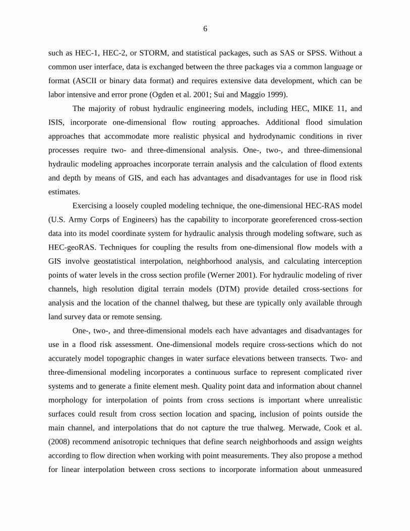
6
such as HEC-1, HEC-2, or STORM, and statistical packages, such as SAS or SPSS. Without a
common user interface, data is exchanged between the three packages via a common language or
format (ASCII or binary data format) and requires extensive data development, which can be
labor intensive and error prone (Ogden et al. 2001; Sui and Maggio 1999).
The majority of robust hydraulic engineering models, including HEC, MIKE 11, and
ISIS, incorporate one-dimensional flow routing approaches. Additional flood simulation
approaches that accommodate more realistic physical and hydrodynamic conditions in river
processes require two- and three-dimensional analysis. One-, two-, and three-dimensional
hydraulic modeling approaches incorporate terrain analysis and the calculation of flood extents
and depth by means of GIS, and each has advantages and disadvantages for use in flood risk
estimates.
Exercising a loosely coupled modeling technique, the one-dimensional HEC-RAS model
(U.S. Army Corps of Engineers) has the capability to incorporate georeferenced cross-section
data into its model coordinate system for hydraulic analysis through modeling software, such as
HEC-geoRAS. Techniques for coupling the results from one-dimensional flow models with a
GIS involve geostatistical interpolation, neighborhood analysis, and calculating interception
points of water levels in the cross section profile (Werner 2001). For hydraulic modeling of river
channels, high resolution digital terrain models (DTM) provide detailed cross-sections for
analysis and the location of the channel thalweg, but these are typically only available through
land survey data or remote sensing.
One-, two-, and three-dimensional models each have advantages and disadvantages for
use in a flood risk assessment. One-dimensional models require cross-sections which do not
accurately model topographic changes in water surface elevations between transects. Two- and
three-dimensional modeling incorporates a continuous surface to represent complicated river
systems and to generate a finite element mesh. Quality point data and information about channel
morphology for interpolation of points from cross sections is important where unrealistic
surfaces could result from cross section location and spacing, inclusion of points outside the
main channel, and interpolations that do not capture the true thalweg. Merwade, Cook et al.
(2008) recommend anisotropic techniques that define search neighborhoods and assign weights
according to flow direction when working with point measurements. They also propose a method
for linear interpolation between cross sections to incorporate information about unmeasured

7
locations. The merging of intricate and accurate channel and floodplain topography produce an
accurate terrain model for flood modeling and groundwater/surface water interaction
investigations. However, the time and expense involved in collecting such high resolution spatial
data may be beyond the scope and budget of many remediation strategies.
Although two- and three-dimensional hydraulic flow models produce descriptive results
for flood analysis, they have high computational requirements and labor-intensive data input
making them difficult to use for decision support systems. The incorporation of higher
dimensions into a hydraulic analysis introduces more uncertainty as the number of assumptions
increases. Rapid assessment of flood impacts is most easily completed with a one-dimensional
hydraulic model, as two- and three-dimensional models require comprehensive data that may not
be readily available for the area of study.
GIS based hydrologic models will likely advance current practices in flood control, flood
mitigation, floodplain mapping, and flood insurance studies. A fully integrated hydrologic and
GIS based system would apply robust modeling techniques and concepts representing spatial and
temporal processes at the same level. GIS provides a powerful tool when coupled with
hydrologic/hydraulic models not only for visualization of flood extents and depths but for further
analysis of flood damage and risk estimates.
1.3 SITE DESCRIPTION
Location
The UBMC is east of Lincoln, Montana in Lewis and Clark County and is located at the
headwaters of the Blackfoot River. The area encompasses several abandoned mines on private
property and the National Forest Service (see Figure 1.1). Once mined for silver, zinc, and lead,
the mines continue to be a source of contamination to local water-ways. The major individual
mines include the Mike Horse Mine, the Anaconda Mine, the Edith Mine, the Paymaster Mine,
and the Carbonate Mine. Smaller mines are located within the Blackfoot River drainage. In
conjunction with a plugged spillway pipe, a 1975 rain-on-snow event lead to a breach in the
Mike Horse tailings impoundment below the Mike Horse Mine. The resulting flood wave
washed tailings down the headwaters of the Blackfoot River (Tate et al. 2002). Combined effects
from the breach and continuous leaching of acid mine drainage from historic mine sites along
tributaries acidified sediments along the floodplain and within a downstream wetland. Within the

8
drainage area, elevations range from 5,200 feet above mean sea level (AMSL) at the marsh
system to 7,500 feet AMSL along the continental divide (Figure 1.1).
Hydrology
Several tributaries contribute runoff to the Blackfoot within the UBMC. The confluence of
Beartrap Creek and Anaconda Creek form the Blackfoot River. Further downstream, the wetland
receives flow from five additional streams (three perennial, two intermittent) during spring
runoff, Shaue Creek, Stevens Gulch, Paymaster Creek, Pass Creek, and Meadow Creek. The
wetland system initiates just upstream of the confluence of the Blackfoot River and Pass Creek
and continues for several miles downstream of the confluence. The total drainage area to the
wetland is 14 square miles. Figure 1.1 denotes drainage areas to the study area.
Climatic data is recorded at the nearby Rogers Pass Station and Lincoln Ranger Station.
Annual precipitation averages are 17.99 inches. The highest annual precipitation in the area was
recorded in 1975 (31.4 inches), the year of the tailings impoundment breach. Until the recent
draining of the reservoir behind the tailings impoundment, water seeped through the earthen dam
and flowed through the overflow pipe during runoff periods maintaining a supply of heavy
metals to downstream tributaries.
Vegetation
The vegetation of the UBMC is characteristic of the Rocky Mountains with some
alterations due to mining activity. The majority of the slopes and transition areas into floodplains
are composed of coniferous forest with lodgepole pine, spruce, and Douglas fir. Mountain big
sagebrush and fescue grassland dominate drier slopes. Wetland and riparian areas within the
study area encompass coniferous and deciduous tree communities as well as shrubs and
herbaceous species. The photos represent vegetation coverage in the marsh study area and
surrounding drainage areas.

9
Geology and Hydrogeology
A mixture of bedrock units are identified within the UBMC, including the Belt Series Spokane
Formation, a diorite sill, and Tertiary-age intrusive bodies. Based on well yield tests, low
bedrock permeability characterizes the site. Permeability is also restricted due to low recharge
areas near the continental divide. Groundwater flows are recharged primarily from snowmelt
from higher elevations to alluvial groundwater systems and tributaries. Major flowpaths include
secondary fractures, joints, and fault zones.
Figure 1.1. The Upper Marsh Study Area (denoted in white above) is located along the
Blackfoot River with several upstream abandoned mines acting as sources of heavy metals
(Data Source: NRIS, MT DEQ)

10
2.0 METHODS AND DATA COLLECTION
The goal of this study was the evaluation of a one-dimensional hydraulic model and the
production of a hazard probability map that encompassed the potential erosive surfaces for the
10, 25, and 100 year recurrence intervals. The identification of drainage areas assisted with the
estimation of flood event discharge values necessary for the hydraulic analysis. A detailed
topographic survey provided the foundational data for the hydraulic model. Soil samples
collected from various points in the wetland by MT DEQ and during field campaigns provided
information on surface roughness and contaminant distributions.
Discharge
Figure 1.2 (A) The Mike Horse Tailings Impoundment is located upstream of Bear Trap
Creek at the headwaters of the Upper Blackfoot River. (B) The upper marsh area is heavily
vegetated and serves as a sink for heavy metals along the Blackfoot River. (C) Pass Creek is a
tributary to the Blackfoot just upstream of the upper marsh area. (D) Velocity measurements
were recorded along reaches to compare to one-dimensional velocity output results.
(A) (B)
(C) (D)

11
Drainage areas (Figure 1.1) for each reach were determined with a GIS. Using the
methods described by Parrett et al. (2004), the drainage area, basin characteristics, annual
precipitation, and active channel width were determined for each reach to estimate discharge
events with 2, 10, 25, 50, 100, 200 and 500 year recurrence intervals. Table 2.1 provides results
from the regression analysis. Discharge estimates were used to parameterize the hydraulic model.
Velocity and stage measurements were taken in each tributary at the same cross section
for thirteen weeks beginning in May and ending in July. Velocity measurements were recorded
every 0.5 ft at a depth six tenths from the bed using a Marsh McBirney. Recorded velocity
measurements across each surveyed cross section provided parameters for an evaluation of the
one-dimensional hydraulic model performance.
Topography and channel geometry
Detailed cross section geometries are necessary to predict flow characteristics in the
wetland, and topographic land surveys were completed using a total station and a survey grade
global positioning system (GPS) device. Variations in topography were also evaluated with an
orthorectified aerial photo and aerial photographs. Using the Delunay triangulation method, an
interpolated surface (TIN) was generated from land survey points and breaklines from the
orthorectified aerial photo. The Delunay triangulation interpolation method had several
advantages: 1) triangles created were as equi-angular as possible, 2) new node values were close
to known observation points, and 3) interpolations were not affected by the sequence of input
data (Hu 1995).
2.1 MODEL DESCRIPTION
The one-dimensional hydraulic model, HEC-RAS, incorporates several parameters to
estimate water surface profiles for steady gradually varied flow. Discharge amounts for each
Anaconda Creek 2.90 13 36 64 129 212 344 538 966
MikeHorse/Bear Trap Creek 1.99 14 37 65 126 200 311 466 784
Shaue Creek 3.28 26 65 109 205 317 485 716 1180
Pass Creek 2.33 24 59 99 185 288 442 653 1080
Paymaster Gulch 0.58 8 21 38 76 122 194 295 506
Meadow Creek 0.64 5 13 24 51 84 135 207 358
Steven's Gulch 0.55 3 10 19 41 69 113 176 311
Qout 1.45 12 32 56 109 173 270 405 680
Drainage Area ID
Drainage
Area (sq.
miles)
2-yr
(cfs)
5-yr
(cfs)
200-yr
(cfs)
500-yr
(cfs)
10-yr
(cfs)
25-yr
(cfs)
50-yr
(cfs)
100-yr
(cfs)
Table 2.1 Drainage areas were estimated for each tributary in the study area and discharges for
flood events were estimated.

12
flood event along contributing reaches and locations of flow changes are required for the
analysis. Surveyed cross section geometries provide detailed topography of the channel and
floodplain areas. The selection of roughness coefficients based on photographs, sediment
samples, and topography transitions is a critical component when incorporating Manning’s
equation to estimate water surface profiles.
One-dimensional hydraulic models are widely used for flood mapping and are typically
simpler to use with minimal amounts of input data in comparison to two- and three-dimensional
models. The U.S. Army Corps of Engineers’ River Analysis System, HEC-RAS, is a robust,
public domain, internationally used hydraulic modeling program. Numerous studies in a variety
of environments, including surface flow through wetlands, have demonstrated HEC-RAS’s
effectiveness in estimating peak discharge (Auble et al. 2005; Johnson et al. 1999). HEC-RAS
calculates one-dimensional, energy-balanced water surface profiles for subcritical and
supercritical conditions. Using an estimated downstream water surface elevation for subcritical
flow, HEC-RAS iteratively determines upstream or downstream water surface profiles. Several
equations are available for calculating channel flow using mass, energy, and momentum
conservation. HEC-RAS has the ability to model an entire network of channels, in either looped
or dendritic configurations.
The model supports several options for incorporating friction equations depending on the
flow regime and profile type. For gradually varied, steady flow estimates, the energy equation is
balanced between successive cross sections. The uniform flow equation, Manning’s equation, is
used to estimate the energy slope at each cross section. To estimate discharges, the Manning
equation combines channel geometry, slope, and an estimate of resistance to flow (roughness
coefficient) to determine stream velocity for turbulent flow on a rough surface. When the
velocity head is rapidly varied (hydraulic jumps, junctions between reaches), the momentum
equation is employed. Further, HEC-RAS offers the capability of entering a roughness
coefficient for each topographic break in a cross-section rather than a single integrated value,
thereby, producing a more accurate representation of spatial variability of roughness across
channel and overbank environments.
Using the energy equation, the robust model estimates water surface profiles between
successive cross sections using the standard step method (Chow 1959). Calculations of flow
depth are carried upstream for subcritical flow and downstream for supercritical flow. An

13
iterative solution calculates unknown water surface elevations at the cross section based on an
assumed water surface elevation, the boundary condition. Total conveyance and velocity head
are used to estimate the friction slope (Sf) and friction head loss (hf).
The energy equation is given by:
(1)
where; y = the thalweg flow depth,
z = the elevation of the channel invert,
α = the velocity head weighting coefficient,
V = the average cross section velocity,
g = the gravitational acceleration, and
he = the head loss.
The friction head loss is estimated through Manning’s equation and accounts for boundary
roughness conditions.
3/4
2
2
2
22
3/4
1
2
2
11
2 RK
nV
RK
nVxxS
nn
f (2)
Δx = the distance between cross sections,
n = Manning’s n,
Kn = the unit correction factor for Manning’s equation, and
R = the hydraulic radius.
The standard step method has several advantages for modeling natural channels. Even if
the water surface elevation is not known at the starting cross section, profile estimates converge
closer to the correct elevation with every step. Therefore, if the elevation at the control section is
unknown, estimates can be made for the initial elevation or computations can begin a few cross
sections away from the desired location.
Manning’s equation assumes uniform flow with consistent channel cross section and
velocity where the energy gradient is equal to the slope of the water surface and stream bed
(Chow 1959). Criticisms of the flow equation include Manning set the exponent of the wetted
perimeter to 2/3 even though his and later research indicates that the value can range from
0.6175 to 0.8395. In addition, the flow equation is dimensionally inhomogeneous and represents
uniform flow rather than non-uniform flow (Pappenberger et al. 2005). The square root of the
slope tends to dampen the uncertainty from energy slopes based on water surface gradient
surveyed in the field.
eh
g
Vzy
g
Vzy
22
2
22
22
2
11
11

14
Selection of Manning’s n Using a Component Method
The combination of calibrated roughness parameters and geometry affect the flood extent
estimates as most hydraulic models are sensitive to these metrics (Marcus et al. 1992;
Pappenberger et al. 2005). Uncertainty arises with approximations of geometry and selection of
roughness values, and it is almost impossible to quantify every source of energy loss in a system.
Roughness coefficients represent the resistance to flood flows in channels and floodplains. Flow
resistance results from sediment size, sediment load, vegetation, sinuosity, contraction and
expansion. Several methods have been developed to estimate values of n, including photographic
comparisons, particle-size based techniques, combinations of roughness generating factors, direct
measurement, and regime equations relating roughness to hydraulic variables (Chow 1959;
Marcus et al. 1992; Pappenberger et al. 2005; Schneider and Arcement 1989).
Roughness coefficients were estimated using the method described by Arcement and
Schneider (1989) for the stream channels and by Cowan (1956) for floodplains. We collected
data for the following parameters: depth of water, sediment size, channel irregularities, changes
in size of channel, channel meanders, obstructions, and vegetation density. Depth and velocity
are two critical factors that will affect the evaluation of flow through the wetland (Kadlec 1990)
and should be considered when selecting a roughness coefficient. Roughness coefficients are
larger if flow depths are small in comparison to the sediment size and decrease with increasing
flow depth if channel banks are not rougher than the bed or if dense vegetation does not intercept
flow in the channel (Schneider and Arcement 1989). The Arcement and Schneider procedure
incorporates the effects of several factors to estimate a roughness coefficient for channel and
floodplain areas. The value of total roughness factor, n, may be computed by the following:
mnnnnnn b )( 4321 (3)
where; nb = a base value of n,
n1 = a correction factor for the effect of surface irregularities,
n2 = a value for variations in shape and size of the channel cross section,
n3 = a value for obstructions,
n4 = a value for vegetation and flow conditions, and
m = a correction factor for channel meandering.
Parameters n1 through n4 are determined through visual observations. Base roughness
values (nb) combine values from Chow (1959), Benson and Dalrymple (1967), and Aldridge and
Garrett (1973). Selecting a base nb value for a channel involves determining if the channel is a

15
stable or sand channel. If the bed consists of firm soil, gravel, cobbles, boulders, or bedrock, it is
classified as stable, while an unlimited supply of sand characterizes a sand channel with grain
sizes ranging from 0.062 to 2mm. Sand bed channel material is transported easily and creates a
resistance to flow with varying bed forms. The movement of sand and the creation of different
configurations is a result of flow velocity, sediment size, bed shear, and temperature.
Floodplain roughness coefficients are estimated with the Cowen method using a similar
procedure for estimating channel roughness. The base roughness value (nb) is selected for the
underlying sediment composition. Adjustment factors for surface irregularities (n1), obstructions
(n3), and vegetation density (n4) are then incorporated into the floodplain roughness coefficient.
The n values for the floodplains are estimated where abrupt changes in resistivity occur,
including topographic breaks, vegetation density, and sediment size changes.
2.2 EROSION
Mine impacted natural wetlands exist in overbank areas throughout Montana, and
evaluating floods for ecosystem impacts aids with making water resource management decisions
(August et al. 2002). Because the mechanism for sediment resuspension in a wetland is erosion,
the dominant controlling factors must be addressed in a model. Soil physical properties,
vegetation, and geomorphology influence friction; therefore, shear stress differs across the
wetland channel and overbank areas (Bendoricchio 2000; Kadlec and Knight 1996).
An essential step for mine-impacted wetland risk assessment is the capability to predict
the impacts of flood events on wetlands (Thompson et al. 2004a). Erosion is a result of increased
forces on soil particles within the channel bed and overbank surfaces and is a function of the
magnitude of resisting channel forces and the hydraulic forces over time (Fischenich et al. 2001).
Predictions of sediment transport and erosion potential depend on empirical equations for natural
channels. Erosion characterization involves predictions of critical shear stress or critical velocity
and is affected by the following parameters: flow properties, sediment composition, climate,
subsurface conditions, channel geometry, biology, and anthropogenic factors. Velocity is a
parameter measured within channel flow; while shear stress is calculated from flow parameters
as a force per unit area. Metals that are resuspended, adsorbed to sediments, or precipitated,
behave as any other sediment in a fluvial environment (Gibbs 1973); therefore, identifying
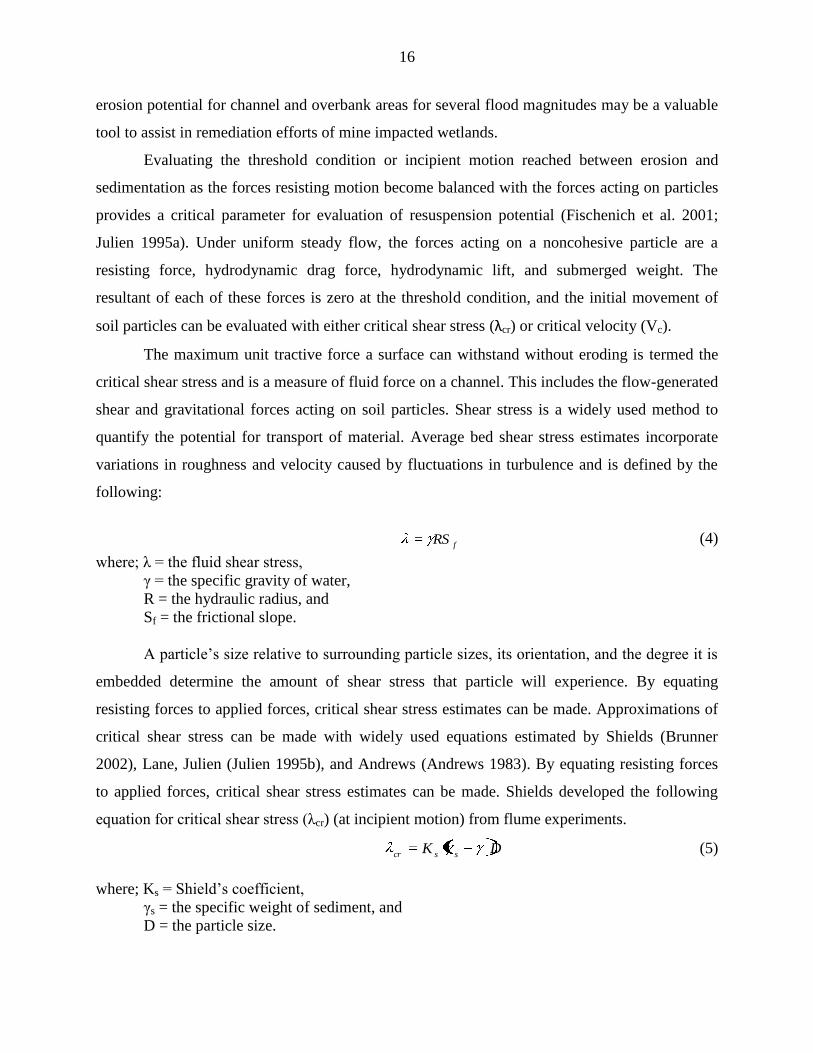
16
erosion potential for channel and overbank areas for several flood magnitudes may be a valuable
tool to assist in remediation efforts of mine impacted wetlands.
Evaluating the threshold condition or incipient motion reached between erosion and
sedimentation as the forces resisting motion become balanced with the forces acting on particles
provides a critical parameter for evaluation of resuspension potential (Fischenich et al. 2001;
Julien 1995a). Under uniform steady flow, the forces acting on a noncohesive particle are a
resisting force, hydrodynamic drag force, hydrodynamic lift, and submerged weight. The
resultant of each of these forces is zero at the threshold condition, and the initial movement of
soil particles can be evaluated with either critical shear stress (λcr) or critical velocity (Vc).
The maximum unit tractive force a surface can withstand without eroding is termed the
critical shear stress and is a measure of fluid force on a channel. This includes the flow-generated
shear and gravitational forces acting on soil particles. Shear stress is a widely used method to
quantify the potential for transport of material. Average bed shear stress estimates incorporate
variations in roughness and velocity caused by fluctuations in turbulence and is defined by the
following:
fRS
(4)
where; λ = the fluid shear stress,
γ = the specific gravity of water,
R = the hydraulic radius, and
Sf = the frictional slope.
A particle’s size relative to surrounding particle sizes, its orientation, and the degree it is
embedded determine the amount of shear stress that particle will experience. By equating
resisting forces to applied forces, critical shear stress estimates can be made. Approximations of
critical shear stress can be made with widely used equations estimated by Shields (Brunner
2002), Lane, Julien (Julien 1995b), and Andrews (Andrews 1983). By equating resisting forces
to applied forces, critical shear stress estimates can be made. Shields developed the following
equation for critical shear stress (λcr) (at incipient motion) from flume experiments.
DK sscr (5)
where; Ks = Shield’s coefficient,
γs = the specific weight of sediment, and
D = the particle size.

17
The hydraulic model estimated average shear stress values for each cross section. Flow
was modeled as subcritical using the normal depth as a boundary condition. Segmented
roughness values across the cross sections in the wetland region and contributing tributaries were
assigned based on sediment size, vegetation coverage, obstructions, and channel meanders. Shear
values were a function of frictional slope, hydraulic radius, and the weight of water and,
therefore, dependent on cross sectional area. Shear stress estimated in the one-dimensional model
is an average shear stress; however, shear stress can also be calculated using log velocity
profiles. The hydraulic radius, a ratio of area to wetted perimeter, heavily influences shear stress
estimates in the hydraulic model. The von Karmen-Prandtl law of velocity distribution (Bergeron
and Abrahams) is another method for estimating shear stress based on log-velocity profiles
plotted as a function of velocity near the channel bed and the natural log of depth over
roughness. Estimating the roughness parameter incorporates uncertainty into shear stress
calculations, but with detailed vertical velocity profiles, the method provides another calibration
estimate for the model.
Critical Velocity
The maximum velocity or critical velocity is the channel velocity that will not permit
erosion, and surpassing the critical velocity results in the initiation of particle motion. An
estimate for critical velocity, developed by Laursen (Akan 2006) is obtained by equating shear
stress to critical shear stress and is based on the concept of tractive force:
2/16/11 DysK
n
KV s
n
c (6)
where: s is the specific gravity of particles (γs/γ). Typical values include 0.039 for Ks and median
diameter (D50) for particle size.
Empirical methods for evaluating velocity and shear stress were developed in flumes.
Natural channels experience high levels of variability and may not experience uniform or steady
flow. The amount of sediment in suspension minimizes turbulence and is not accounted for in the
given estimates of velocity and shear stress. Variation in particle size influences stress in
channels. Larger particles often inhibit smaller particles from motion until significant flows and
higher stress are experienced. Application of this method to our data required the assumption that
flow is steady and the use of an interpolated median particle size distribution.
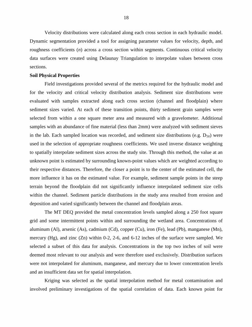
18
Velocity distributions were calculated along each cross section in each hydraulic model.
Dynamic segmentation provided a tool for assigning parameter values for velocity, depth, and
roughness coefficients (n) across a cross section within segments. Continuous critical velocity
data surfaces were created using Delaunay Triangulation to interpolate values between cross
sections.
Soil Physical Properties
Field investigations provided several of the metrics required for the hydraulic model and
for the velocity and critical velocity distribution analysis. Sediment size distributions were
evaluated with samples extracted along each cross section (channel and floodplain) where
sediment sizes varied. At each of these transition points, thirty sediment grain samples were
selected from within a one square meter area and measured with a gravelometer. Additional
samples with an abundance of fine material (less than 2mm) were analyzed with sediment sieves
in the lab. Each sampled location was recorded, and sediment size distributions (e.g. D50) were
used in the selection of appropriate roughness coefficients. We used inverse distance weighting
to spatially interpolate sediment sizes across the study site. Through this method, the value at an
unknown point is estimated by surrounding known-point values which are weighted according to
their respective distances. Therefore, the closer a point is to the center of the estimated cell, the
more influence it has on the estimated value. For example, sediment sample points in the steep
terrain beyond the floodplain did not significantly influence interpolated sediment size cells
within the channel. Sediment particle distributions in the study area resulted from erosion and
deposition and varied significantly between the channel and floodplain areas.
The MT DEQ provided the metal concentration levels sampled along a 250 foot square
grid and some intermittent points within and surrounding the wetland area. Concentrations of
aluminum (Al), arsenic (As), cadmium (Cd), copper (Cu), iron (Fe), lead (Pb), manganese (Mn),
mercury (Hg), and zinc (Zn) within 0-2, 2-6, and 6-12 inches of the surface were sampled. We
selected a subset of this data for analysis. Concentrations in the top two inches of soil were
deemed most relevant to our analysis and were therefore used exclusively. Distribution surfaces
were not interpolated for aluminum, manganese, and mercury due to lower concentration levels
and an insufficient data set for spatial interpolation.
Kriging was selected as the spatial interpolation method for metal contamination and
involved preliminary investigations of the spatial correlation of data. Each known point for
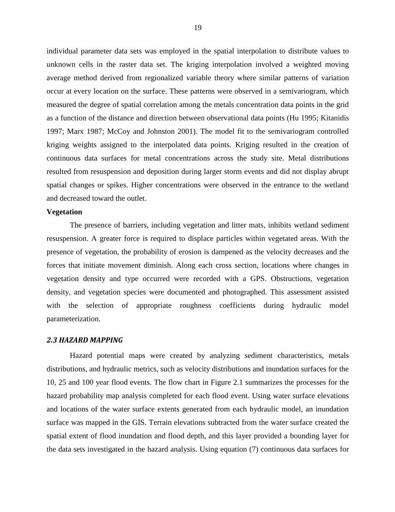
19
individual parameter data sets was employed in the spatial interpolation to distribute values to
unknown cells in the raster data set. The kriging interpolation involved a weighted moving
average method derived from regionalized variable theory where similar patterns of variation
occur at every location on the surface. These patterns were observed in a semivariogram, which
measured the degree of spatial correlation among the metals concentration data points in the grid
as a function of the distance and direction between observational data points (Hu 1995; Kitanidis
1997; Marx 1987; McCoy and Johnston 2001). The model fit to the semivariogram controlled
kriging weights assigned to the interpolated data points. Kriging resulted in the creation of
continuous data surfaces for metal concentrations across the study site. Metal distributions
resulted from resuspension and deposition during larger storm events and did not display abrupt
spatial changes or spikes. Higher concentrations were observed in the entrance to the wetland
and decreased toward the outlet.
Vegetation
The presence of barriers, including vegetation and litter mats, inhibits wetland sediment
resuspension. A greater force is required to displace particles within vegetated areas. With the
presence of vegetation, the probability of erosion is dampened as the velocity decreases and the
forces that initiate movement diminish. Along each cross section, locations where changes in
vegetation density and type occurred were recorded with a GPS. Obstructions, vegetation
density, and vegetation species were documented and photographed. This assessment assisted
with the selection of appropriate roughness coefficients during hydraulic model
parameterization.
2.3 HAZARD MAPPING
Hazard potential maps were created by analyzing sediment characteristics, metals
distributions, and hydraulic metrics, such as velocity distributions and inundation surfaces for the
10, 25 and 100 year flood events. The flow chart in Figure 2.1 summarizes the processes for the
hazard probability map analysis completed for each flood event. Using water surface elevations
and locations of the water surface extents generated from each hydraulic model, an inundation
surface was mapped in the GIS. Terrain elevations subtracted from the water surface created the
spatial extent of flood inundation and flood depth, and this layer provided a bounding layer for
the data sets investigated in the hazard analysis. Using equation (7) continuous data surfaces for

20
water depth, flow velocity, and sediment size for each of the flood events of interest were
combined to produce spatially continuous critical velocity layers. These layers were then
overlaid by modeled velocity distributions to obtain a percent exceedance value. For any given
cell on the hazard potential map, percent exceedance was calculated as follows:
(Vm / Vc )*100 (7)
where; Vm = modeled velocity
Vc = critical velocity
Results of the percent exceedance map suggest areas where the modeled flood velocity is
likely to exceed the threshold condition at which sediment is mobilized. Combining the percent
exceedance data with data surfaces for contaminant distributions of arsenic (As), copper (Cu),
cadmium (Cd), lead (Pb), and zinc (Zn) allows for the creation of hazard potential maps. These
maps provide a qualitative visual tool for assessing the spatial distribution of sediment
contamination and the estimated percent velocity exceedance simultaneously.
2.4 SENSITIVITY ANALYSIS AND ERROR CHECKING
Evaluation of the hydrologic and hydraulic performance of the model within a dynamic
wetland situation was conducted by testing the accuracy and stability of the output in a
sensitivity analysis. In particular, alterations to roughness coefficients, contraction/expansion
coefficients, and spacing of cross-sections addressed the dependence of the output on specific
input variables communicates the model’s limitations. Manning’s roughness coefficients were
globally altered by 10%, -10%, 25%, and -25%. Contraction/expansion coefficients were
adjusted from 0.1/0.3 to 0/0.5, 0/0, and 0.3/0.7. By adjusting the spacing of cross-sections
through interpolation or removal, shortcomings in our topographic survey were identified.
Velocity distribution results from the hydraulic model for selected cross sections were compared
to field velocity measurements.
Metal concentration distributions were spatially interpolated with ordinary kriging and
spherical models. The spherical models were fit using a Monte Carlo analysis which provided
parameter sets that minimized the sum of squared errors. Kriging provides estimates of error
variance for the interpolated contamination levels within the wetland.

21
Se
dim
en
t
Siz
e (
D5
0)
(Ve
cto
r)
Co
nta
min
an
t
Le
ve
ls
(Ve
cto
r)
Se
dim
en
t
Ra
ste
r
Co
nta
min
an
t
Ra
ste
r
Ha
za
rd M
ap
Ra
ste
r
Bo
un
ds a
ll la
ye
rs
Sp
atia
l
Inte
rpo
latio
n
(In
ve
rse
Dis
tan
ce
We
igh
tin
g)
Sp
atia
l
Inte
rpo
latio
n
(Krig
ing
)
Imp
ort
hyd
rau
lic
an
aly
sis
resu
lts to
GIS
Cre
ate
X-s
ectio
n
cu
t lin
es w
ith
wa
ter
su
rfa
ce
ele
v.
(Ve
cto
r)
Cre
ate
bo
un
din
g
po
lyg
on
(V
ecto
r)
Cre
ate
Ra
ste
r o
f
DT
M
Wa
ter
su
rfa
ce
TIN
(Ve
cto
r)
Wa
ter
Su
rfa
ce
Ra
ste
r
Co
mp
are
wa
ter
su
rfa
ce
ra
ste
r w
ith
DT
M r
aste
r
Inu
nd
atio
n
de
pth
ra
ste
r
Cre
ate
flo
od
pla
in
bo
un
da
ry p
oly
go
n
(Ve
cto
r)
Eva
lua
te r
esu
lts
for
hyd
rau
lic s
en
se
DT
M (
TIN
)
La
nd
su
rve
y
po
ints
(Ve
cto
r)
Ge
ne
rate
X-
se
ctio
n
ge
om
etr
ies/
exp
ort
to H
EC
-RA
S
Hyd
rau
lic a
na
lysis
Ve
locity
Ra
ste
r
Critica
l V
elo
city
Ra
ste
r
Ro
ug
hn
ess
Co
effic
ien
t
Ra
ste
r
Flo
w D
ep
th
Ra
ste
r
Co
mp
are
V to
VC
An
aly
sis
of V
c
exce
ed
an
ce
with
[Me
tal]
Figu
re 2
.1.
The
haz
ard
pro
bab
ility
map
flo
w c
har
t d
escr
ibes
th
e p
roce
sses
an
d d
ata
sets
req
uir
ed
fo
r an
alys
is i
n t
he
GIS
an
d
hyd
rau
lic m
od
el.
Se
dim
en
t
Siz
e (
D5
0)
(Ve
cto
r)
Co
nta
min
an
t
Le
ve
ls
(Ve
cto
r)
Se
dim
en
t
Ra
ste
r
Co
nta
min
an
t
Ra
ste
r
Ha
za
rd M
ap
Ra
ste
r
Bo
un
ds a
ll la
ye
rs
Sp
atia
l
Inte
rpo
latio
n
(In
ve
rse
Dis
tan
ce
We
igh
tin
g)
Sp
atia
l
Inte
rpo
latio
n
(Krig
ing
)
Imp
ort
hyd
rau
lic
an
aly
sis
resu
lts to
GIS
Cre
ate
X-s
ectio
n
cu
t lin
es w
ith
wa
ter
su
rfa
ce
ele
v.
(Ve
cto
r)
Cre
ate
bo
un
din
g
po
lyg
on
(V
ecto
r)
Cre
ate
Ra
ste
r o
f
DT
M
Wa
ter
su
rfa
ce
TIN
(Ve
cto
r)
Wa
ter
Su
rfa
ce
Ra
ste
r
Co
mp
are
wa
ter
su
rfa
ce
ra
ste
r w
ith
DT
M r
aste
r
Inu
nd
atio
n
de
pth
ra
ste
r
Cre
ate
flo
od
pla
in
bo
un
da
ry p
oly
go
n
(Ve
cto
r)
Eva
lua
te r
esu
lts
for
hyd
rau
lic s
en
se
DT
M (
TIN
)
La
nd
su
rve
y
po
ints
(Ve
cto
r)
Ge
ne
rate
X-
se
ctio
n
ge
om
etr
ies/
exp
ort
to H
EC
-RA
S
Hyd
rau
lic a
na
lysis
Ve
locity
Ra
ste
r
Critica
l V
elo
city
Ra
ste
r
Ro
ug
hn
ess
Co
effic
ien
t
Ra
ste
r
Flo
w D
ep
th
Ra
ste
r
Co
mp
are
V to
VC
An
aly
sis
of V
c
exce
ed
an
ce
with
[Me
tal]
Figu
re 2
.1.
The
haz
ard
pro
bab
ility
map
flo
w c
har
t d
escr
ibes
th
e p
roce
sses
an
d d
ata
sets
req
uir
ed
fo
r an
alys
is i
n t
he
GIS
an
d
hyd
rau
lic m
od
el.

22
3.0 RESULTS AND DISCUSSION
3.1 HYDRAULIC ANALYSIS
The one-dimensional model estimated water surface elevations and hydraulic parameters
for calculations of critical velocity. Detailed roughness parameters based on sediment size and
vegetation were used to estimate flow across cross sections and, therefore, water surface
elevations and velocity distributions. Some cross sections required critical depth determination
when the energy equation failed to balance within a specific number of iterations.
Estimates of water surface elevations within the natural channel in the one-dimensional
hydraulic model involve several assumptions. Flow was assumed to be steady throughout the
reach and to be gradually varied between cross sections as the energy equation is based on the
theory of a hydrostatic pressure distribution across each cross section. Cross sections were
located along a given reach and satisfied the gradually varied flow assumption. Flow was
considered to be one-dimensional and in the dominant flow direction without considering
velocity in any other direction. The total energy head was assumed to be the same at every point
along a cross section. The energy slope was assumed to be uniform across any given cross
section and between consecutive cross sections.
Velocity distributions in HEC-RAS calculated for a set number of divisions across a
cross section are a function of conveyance and area for each subdivision. Velocity in a natural
channel varies vertically and horizontally, and output from the one-dimensional model is an
average velocity for each segmented area within the channel. Velocity distributions typically
Anaconda Creek 2223 16
Blackfoot Reach 1 (MikeHorse/Bear Trap Creek) 3641 35
Blackfoot Reach 2 4993 70
Shaue Creek 1392 8
Blackfoot Reach 3 4724 28
Pass Creek 1563 8
Blackfoot Reach 4 4487 17
Meadow Creek 1878 5
Blackfoot Reach 5 2448 11
Drainage Area IDNumber of
Cross Sections
Reach
Length
(ft)
Table 3.1. Nine reaches within the study area were modeled with at least five cross sections
to estimate water surface elevations.
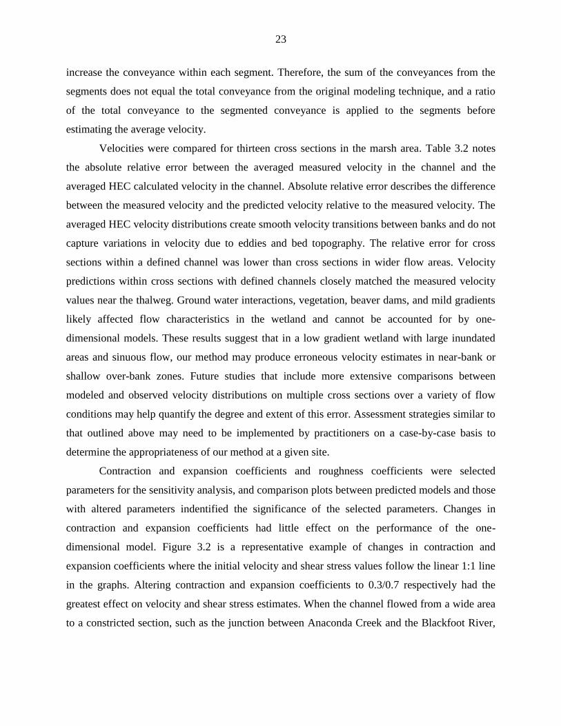
23
increase the conveyance within each segment. Therefore, the sum of the conveyances from the
segments does not equal the total conveyance from the original modeling technique, and a ratio
of the total conveyance to the segmented conveyance is applied to the segments before
estimating the average velocity.
Velocities were compared for thirteen cross sections in the marsh area. Table 3.2 notes
the absolute relative error between the averaged measured velocity in the channel and the
averaged HEC calculated velocity in the channel. Absolute relative error describes the difference
between the measured velocity and the predicted velocity relative to the measured velocity. The
averaged HEC velocity distributions create smooth velocity transitions between banks and do not
capture variations in velocity due to eddies and bed topography. The relative error for cross
sections within a defined channel was lower than cross sections in wider flow areas. Velocity
predictions within cross sections with defined channels closely matched the measured velocity
values near the thalweg. Ground water interactions, vegetation, beaver dams, and mild gradients
likely affected flow characteristics in the wetland and cannot be accounted for by one-
dimensional models. These results suggest that in a low gradient wetland with large inundated
areas and sinuous flow, our method may produce erroneous velocity estimates in near-bank or
shallow over-bank zones. Future studies that include more extensive comparisons between
modeled and observed velocity distributions on multiple cross sections over a variety of flow
conditions may help quantify the degree and extent of this error. Assessment strategies similar to
that outlined above may need to be implemented by practitioners on a case-by-case basis to
determine the appropriateness of our method at a given site.
Contraction and expansion coefficients and roughness coefficients were selected
parameters for the sensitivity analysis, and comparison plots between predicted models and those
with altered parameters indentified the significance of the selected parameters. Changes in
contraction and expansion coefficients had little effect on the performance of the one-
dimensional model. Figure 3.2 is a representative example of changes in contraction and
expansion coefficients where the initial velocity and shear stress values follow the linear 1:1 line
in the graphs. Altering contraction and expansion coefficients to 0.3/0.7 respectively had the
greatest effect on velocity and shear stress estimates. When the channel flowed from a wide area
to a constricted section, such as the junction between Anaconda Creek and the Blackfoot River,

24
shear stress values increased. Error estimates for the flood events indicate that larger flood events
are less affected by changes in contraction and expansion coefficients.
Absolute Relative
Error
Average Measured
Velocity in Channel
Average HEC Calculated
Velocity in Channel(%) (ft/s) (ft/s)
11943 60 0.89 1.43
11633 386 0.40 1.96
10889 8 1.75 1.61
10184 24 1.15 0.87
9762 2 1.03 1.05
9566 151 0.59 1.49
9399 23 0.82 1.01
8594 6 0.74 0.79
7844 35 1.18 0.77
5674 412 0.41 2.12
5387 434 0.39 2.07
4463 13 0.69 0.60
2821 59 0.18 0.29
Cross Section
Velocity Distribution Cross Section 9399.322
0.00
0.20
0.40
0.60
0.80
1.00
1.20
1.40
1.60
434 436 438 440 442 444 446
Station (ft)
Velo
cit
y (
ft/s
)
Measured Velocity HEC Velocity
Figure 3.1. Velocity distributions at one foot increments across a defined cross section are
similar near the thalweg (Station 438) but differ at the edges of the channel water surface.
Table 3.2. Absolute relative error between average measured velocities and HEC average velocity
output vary at thirteen locations in the wetland.
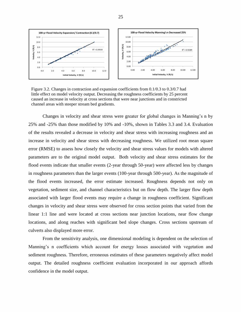
25
Changes in velocity and shear stress were greater for global changes in Manning’s n by
25% and -25% than those modified by 10% and -10%, shown in Tables 3.3 and 3.4. Evaluation
of the results revealed a decrease in velocity and shear stress with increasing roughness and an
increase in velocity and shear stress with decreasing roughness. We utilized root mean square
error (RMSE) to assess how closely the velocity and shear stress values for models with altered
parameters are to the original model output. Both velocity and shear stress estimates for the
flood events indicate that smaller events (2-year through 50-year) were affected less by changes
in roughness parameters than the larger events (100-year through 500-year). As the magnitude of
the flood events increased, the error estimate increased. Roughness depends not only on
vegetation, sediment size, and channel characteristics but on flow depth. The larger flow depth
associated with larger flood events may require a change in roughness coefficient. Significant
changes in velocity and shear stress were observed for cross section points that varied from the
linear 1:1 line and were located at cross sections near junction locations, near flow change
locations, and along reaches with significant bed slope changes. Cross sections upstream of
culverts also displayed more error.
From the sensitivity analysis, one dimensional modeling is dependent on the selection of
Manning’s n coefficients which account for energy losses associated with vegetation and
sediment roughness. Therefore, erroneous estimates of these parameters negatively affect model
output. The detailed roughness coefficient evaluation incorporated in our approach affords
confidence in the model output.
R² = 0.9939
0.0
2.0
4.0
6.0
8.0
10.0
12.0
0.0 2.0 4.0 6.0 8.0 10.0 12.0
Ve
loci
ty, V
(ft
/s)
Initial Velocity, V (ft/s)
100-yr Flood Velocity Expansion/ Contraction (0.3/0.7)
R² = 0.9289
0.00
2.00
4.00
6.00
8.00
10.00
12.00
0.00 2.00 4.00 6.00 8.00 10.00 12.00
Ve
loci
ty, V
(ft
/s)
Initial Velocity, V (ft/s)
100-yr Flood Velocity Manning's n Decreased 25%
Figure 3.2. Changes in contraction and expansion coefficients from 0.1/0.3 to 0.3/0.7 had
little effect on model velocity output. Decreasing the roughness coefficients by 25 percent
caused an increase in velocity at cross sections that were near junctions and in constricted
channel areas with steeper stream bed gradients.
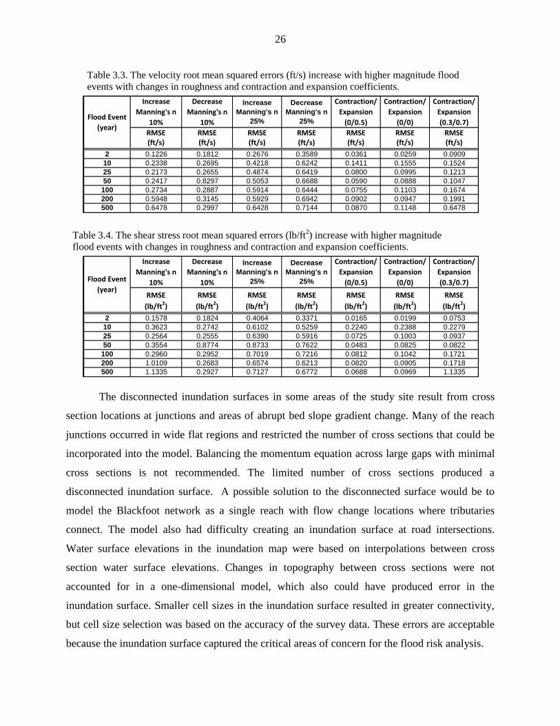
26
The disconnected inundation surfaces in some areas of the study site result from cross
section locations at junctions and areas of abrupt bed slope gradient change. Many of the reach
junctions occurred in wide flat regions and restricted the number of cross sections that could be
incorporated into the model. Balancing the momentum equation across large gaps with minimal
cross sections is not recommended. The limited number of cross sections produced a
disconnected inundation surface. A possible solution to the disconnected surface would be to
model the Blackfoot network as a single reach with flow change locations where tributaries
connect. The model also had difficulty creating an inundation surface at road intersections.
Water surface elevations in the inundation map were based on interpolations between cross
section water surface elevations. Changes in topography between cross sections were not
accounted for in a one-dimensional model, which also could have produced error in the
inundation surface. Smaller cell sizes in the inundation surface resulted in greater connectivity,
but cell size selection was based on the accuracy of the survey data. These errors are acceptable
because the inundation surface captured the critical areas of concern for the flood risk analysis.
Increase
Manning's n
10%
Decrease
Manning's n
10%
Increase
Manning's n
25%
Decrease
Manning's n
25%
Contraction/
Expansion
(0/0.5)
Contraction/
Expansion
(0/0)
Contraction/
Expansion
(0.3/0.7)
RMSE RMSE RMSE RMSE RMSE RMSE RMSE(ft/s) (ft/s) (ft/s) (ft/s) (ft/s) (ft/s) (ft/s)
2 0.1226 0.1812 0.2676 0.3589 0.0361 0.0259 0.0909
10 0.2338 0.2695 0.4218 0.6242 0.1411 0.1555 0.1524
25 0.2173 0.2655 0.4874 0.6419 0.0800 0.0995 0.1213
50 0.2417 0.8297 0.5053 0.6688 0.0590 0.0888 0.1047
100 0.2734 0.2887 0.5914 0.6444 0.0755 0.1103 0.1674
200 0.5948 0.3145 0.5929 0.6942 0.0902 0.0947 0.1991
500 0.6478 0.2997 0.6428 0.7144 0.0870 0.1148 0.6478
Flood Event
(year)
Increase
Manning's n
10%
Decrease
Manning's n
10%
Increase
Manning's n
25%
Decrease
Manning's n
25%
Contraction/
Expansion
(0/0.5)
Contraction/
Expansion
(0/0)
Contraction/
Expansion
(0.3/0.7)
RMSE RMSE RMSE RMSE RMSE RMSE RMSE
(lb/ft2) (lb/ft2) (lb/ft2) (lb/ft2) (lb/ft2) (lb/ft2) (lb/ft2)
2 0.1578 0.1824 0.4064 0.3371 0.0165 0.0199 0.0753
10 0.3623 0.2742 0.6102 0.5259 0.2240 0.2388 0.2279
25 0.2564 0.2555 0.6390 0.5916 0.0725 0.1003 0.0937
50 0.3554 0.8774 0.8733 0.7622 0.0483 0.0825 0.0822
100 0.2960 0.2952 0.7019 0.7216 0.0812 0.1042 0.1721
200 1.0109 0.2683 0.6574 0.6213 0.0820 0.0905 0.1718
500 1.1335 0.2927 0.7127 0.6772 0.0688 0.0969 1.1335
Flood Event
(year)
Table 3.4. The shear stress root mean squared errors (lb/ft2) increase with higher magnitude
flood events with changes in roughness and contraction and expansion coefficients.
Table 3.3. The velocity root mean squared errors (ft/s) increase with higher magnitude flood
events with changes in roughness and contraction and expansion coefficients.
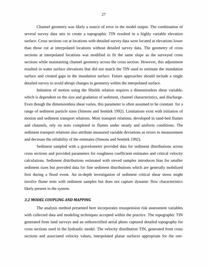
27
Channel geometry was likely a source of error in the model output. The combination of
several survey data sets to create a topographic TIN resulted in a highly variable elevation
surface. Cross sections cut at locations with detailed survey data were located at elevations lower
than those cut at interpolated locations without detailed survey data. The geometry of cross
sections at interpolated locations was modified to fit the same slope as the surveyed cross
sections while maintaining channel geometry across the cross section. However, this adjustment
resulted in water surface elevations that did not match the TIN used to estimate the inundation
surface and created gaps in the inundation surface. Future approaches should include a single
detailed survey to avoid abrupt changes in geometry within the interpolated surface.
Initiation of motion using the Shields relation requires a dimensionless shear variable,
which is dependent on the size and gradation of sediment, channel characteristics, and discharge.
Even though the dimensionless shear varies, this parameter is often assumed to be constant for a
range of sediment particle sizes (Simons and Sentürk 1992). Limitations exist with initiation of
motion and sediment transport relations. Most transport relations, developed in sand-bed flumes
and channels, rely on tests completed in flumes under steady and uniform conditions. The
sediment transport relations also attribute measured variable deviations as errors in measurement
and decrease the reliability of the estimates (Simons and Sentürk 1992).
Sediment sampled with a gravelometer provided data for sediment distributions across
cross sections and provided parameters for roughness coefficient estimates and critical velocity
calculations. Sediment distributions estimated with sieved samples introduces bias for smaller
sediment sizes but provided data for fine sediment distributions which are generally mobilized
first during a flood event. An in-depth investigation of sediment critical shear stress might
involve flume tests with sediment samples but does not capture dynamic flow characteristics
likely present in the system.
3.2 MODEL COUPLING AND MAPPING
The analysis method presented here incorporates resuspension risk assessment variables
with collected data and modeling techniques accepted within the practice. The topographic TIN
generated from land surveys and an orthorectified aerial photo captured detailed topography for
cross sections used in the hydraulic model. The velocity distribution TIN, generated from cross
sections and associated velocity values, interpolated planar surfaces appropriate for the one-

28
dimensional hydraulic model output. Since velocity values at cross sections vary significantly
due to changes in channel slope, cross section geometry, and roughness factors, the planar
surfaces of velocity values between the cross sections maintained velocity values along the cross
sections.
Spatial interpolation of sample points is a common decision making tool for soil
remediation and erosion and deposition studies. Soil properties and contaminant distributions are
difficult to model and track even with a large number of sample points in such a heterogeneous
system. The spatial interpolation tools in the GIS produce distribution surfaces that can be used
for making cost-efficient decisions for remediation strategies, but the results of spatial analysis
differ with interpolation techniques.
Spatial interpolation introduces uncertainty to modeling. Attempts to minimize
uncertainty included selecting interpolation methods appropriate for the data type. Kriging of
contamination sample points attempted to reduce interpolation bias by assigning weights to
observational points dependent on distances between the points and estimation locations as well
as mutual distances among observational points. Semivariograms helped to assess the spatial
dependency of observational data points in which a functional relationship between the spatial
pattern of the sampled points and their observed values was defined. Semivariograms for arsenic,
cadmium, copper, zinc, and lead concentrations were fit with a spherical model (see Figure 3.3),
and parameters from the model were used to interpolate a kriged contamination surface. The
error variance for each kriged surface indicates higher variance further from known points. In
particular, the error variance was high at the edges of the surface where fewer points were used
to interpolate values across the grid. However, most of these areas were beyond the bounding
inundation surface and likely had little effect on our results.

29
For the 10, 25, and 100 year flood events, the combination of distribution maps for
velocity, critical velocity, sediment size, flood extents, and metal contamination (As, Cu, Cd, Pb,
and Zn) help identify areas of potential concern in the wetland. An analysis of the metals of
potential concern identified areas where specific metals exceeded preliminary remediation goals
for residential screening levels and ecological screening levels. Table 3.5 lists the DEQ and
Environmental Protection Agency (EPA) remediation goals for the site.
The velocity surface was compared to the critical velocity surface, and areas where the velocity
exceeded the critical velocity were identified. Percentages of velocity exceeding critical velocity
were high within the wetland study area and were indicated with a three-dimension elevation
map. Spikes in Figure 3.4 indicate areas where velocities exceed critical velocities. Figure 3.4
demonstrates the hazardous areas for the 100 year flood event along with arsenic concentration
distributions. For the 10, 25, and 100 year events, estimated velocities exceed critical velocity by
97 percent, 99 percent, and 76 percent, respectively, in the study area (see Table 3.6). Results
from the potential hazard analysis indicate increasing hazard regions with larger flood events.
Metal concentrations are higher at the entrance of the wetland where tributaries intersect and
where the flood wave from the 1975 breach event lost energy and deposited sediment.
Figure 3.3. The semivariogram for sampled sediment containing arsenic, fit
with a spherical model, demonstrates the decreasing similarity of data
points (blue dots) with increasing distance from known points.

30
4.0 CONCLUSION
Water resource problems, in particular, flood inundation mapping, rely on robust
hydrologic and hydraulic models such as HEC-RAS. Intricate analysis and simulation
Aluminum Arsenic Cadmium Copper Lead Mercury Manganese Zinc
(mg/kg) (mg/kg) (mg/kg) (mg/kg) (mg/kg) (mg/kg) (mg/kg) (mg/kg)
Residential PRG 77,000 40a
37b
3,100b
400b
230b
1.800b
23,000b
TELc
-- 5.9 0.596 35.7 35 0.174 -- 123
PAETc
-- 19 97.5 340 240 0.16 1,400 500
SELc
-- 33 10 110 250 2 1,100 820
Metal
Flood Event
(year)
Total Area Inundated by 100yr
flood in the Upper Marsh
Area Velocity Exceeds
Critical VelocityPercent of Total Marsh
Area where V>Vc
(acres) (acres) (%)
100 57 43 76
25 38 38 99
10 28 27 98
N
As concentration (mg/kg)
0 - 9
10 - 14
15 - 20
21 - 44
45 - 235
As concentration
(mg/kg)
Projection: NAD 1983 Montana State Plane
Data Source: MT DEQ
975
1230
670480
420
Figure 3.4. For a 100-year flood event, areas of potential concern include those where spikes
occur in the surface identifying the magnitude of velocities exceeding critical velocities and
those where contaminant sediment levels are significant.
Table 3.6. A comparison of the upper marsh area indicates areas where velocities for the 10, 25,
and 100 year flood events exceed critical velocities.
Table 3.5. The summary of EPA Region 9 Preliminary Remediation Goals for comparison with
soil, mine waste, and tailings sample data assisted with identifying areas where metal
concentration levels exceeded screening levels in the upper marsh study area. a DEQ Action Level for Arsenic in Surface Soil (DEQ Remediation Division, 2005).
b EPA Region 9 Preliminary Remediation Goals (PRGs) for residential soil (October 2004).
c Percentile screening levels for biological effects.

31
capabilities are available with both hydrologic/hydraulic models and GIS, and the integration of
the two provides a powerful tool for scientific researchers and policy makers. The widespread
availability of spatially distributed data through GIS has made physically based hydrologic
models more useable and spurred the development of hydrologic models that take advantage of
these new data. This approach for evaluating the potential hazards of metals-trapping wetlands
will aid the MT DEQ and the US Forest Service in prioritizing and implementing remediation
action items for the UBMC and similar mine reclamation sites. In this study, the coupling of GIS
and a hydraulic model through HEC-geoRAS produced an inundation surface only after
numerous modeling iterations. The disconnected stream flow results resulted from cell size
selection and were influenced by the wide shallow topography of the site. The inundation surface
bounded resuspension parameters, critical velocity, sediment size, and metal contamination to
model areas of possible resuspension risk. Providing agencies, consultants, and watershed groups
with a viable, low cost, computationally efficient method with minimal data requirements for
quantifying the risk associated with transport of contaminated sediments out of wetlands will aid
these entities in prioritization of restoration efforts and help reduce mining impacts to
downstream communities and environments.
Despite the complex nature of the wetland system, the one-dimensional hydraulic model
proved to be a sufficient tool to estimate the water surface elevations and flow parameters.
Sensitivity analysis showed the one-dimensional hydraulic model to be increasingly sensitive to
roughness coefficients at larger discharges. This highlights the need for careful characterization
and mapping of roughness values if large flood events are being modeled. Comparison of
modeled stream velocity distributions to measured velocity distributions showed deviations from
observed data in shallow near-bank and over-bank areas. Further investigation is needed in this
area to quantify the effect of these deviations on model output for a variety of discharge events.
Thorough investigation of differences between modeled and measured velocity distributions at a
range of flows and across several transects at a given site will help practitioners decide whether
or not this approach will be useful and may improve confidence in modeled output. We conclude
that, if carefully applied, this approach may be a valuable tool for coarse assessments of
contaminated sediment mobilization risk in areas where data is limited and/or development of
more data/computationally intensive sediment transport, 2D or 3D models is not feasible.

32
REFERENCES
Akan, A. O. (2006). Open Channel Hydraulics, Elsevier, Burlington, MA.
Aldridge, B. N., Garrett, J. M., and Highway, D. (1973). Roughness Coefficients for Stream
Channels in Arizona, US Dept. of the Interior, US Geological Survey.
Andrews, E. D. (1983). "Entrainment of gravel from naturally sorted riverbed material." Bulletin
of the Geological Society of America, 94(10), 1225-1231.
Auble, G. T., Scott, M. L., and Friedman, J. M. (2005). "Use of individualistic streamflow-
vegetation relations along the Fremont River, Utah, USA to assess impacts of flow
alteration on wetland and riparian areas." Wetlands, 25(1), 143-154.
August, E. E., McKnight, D. M., Hrncir, D. C., and Garhart, K. S. (2002). "Seasonal variability
of metals transport through a wetland impacted by mine drainage in the Rocky
Mountains." Environmental Science & Technology, 36(17), 3779-3786.
Bendoricchio, G., Luigi Dal Cin, and Jesper Persson. (2000). "Guidelines for free water surface
wetland design." ECOSYSTEMS, 8, 51-91.
Benson, M. A., and Dalrymple, T. (1967). "GENERAL FIELD AND OFFICE PROCEDURES
FOR INDIRECT DISCHARGE MEASUREMENTS."
Bergeron, N. E., and Abrahams, A. D. "Estimating shear velocity and roughness length from
velocity profiles." WATER RESOUR RES, 28(8).
Brunner, G. W. (2002). "HEC-RAS, River Analysis System Hydraulic Reference Manual,
Version 3.1." In: US Army Corps of Engineers, Hydrologic Engineering Center, CPD-69,
1-377.
Chow, V. T. (1959). "Open-channel hydraulics." In: New York/Tokyo, McGraw-Hill, 680.
Cook, S. A. (2007). "Characterization of riparian wetland soils and associated metal
concentrations at the headwaters of the Stillwater River, Montana," Montana State
University, Bozeman, MT.
Dollhopf, D. J., Goering, J. D., Rennick, R. B., Morton, R. B., Gauger, W. K., Guckert, J. B.,
Jones, P. B., Cooksey, K. C., Bucklin, K. E., Weed, R., and Lehman, M. M. (1988).
"Hydrochemical, vegetational and microbiological effects of a natural and constructed
wetland on the control of acid mine drainage." RRU 8804, Montana Abandoned Mine
Reclamation Bureau, Helena, MT.
Fischenich, C., Engineer, R., and Development Center Vicksburg Ms Environmental, L. A. B.
(2001). "Stability Thresholds for Stream Restoration Materials." ENGINEER
RESEARCH AND DEVELOPMENT CENTER VICKSBURG MS
ENVIRONMENTAL LAB.
Furniss, G., Hinman, N. W., Doyle, G. A., and Runnells, D. D. (1999). "Radiocarbon-dated
ferricrete provides a record of natural acid rock drainage and paleoclimatic changes."
Environmental Geology, 37(1), 102-106.
Gibbs, R. J. (1973). "Mechanisms of Trace Metal Transport in Rivers." Science, 180(4081), 71-
73.
Gurrieri, J. T. (1998). "Distribution of metals in water and sediment and effects on aquatic biota
in the upper Stillwater River basin, Montana." Journal of Geochemical Exploration,
64(1-3), 83-100.

33
Haag, I., Kern, U., and Westrich, B. (2001). "Erosion investigation and sediment quality
measurements for a comprehensive risk assessment of contaminated aquatic sediments."
Science of the Total Environment, The, 266(1-3), 249-257.
Hu, J. (Year). "Methods of Generating Surfaces In Environmental GIS Applications." 22-26.11.
Johnson, G. D., Strickland, M. D., Buyok, J. P., Derby, C. E., and Young, D. P. (1999). "
Quantifying impacts to riparian wetlands associated with reduced flows along the
Greybull River, Wyoming " Wetlands, 19(1), 71-77.
Julien, P. Y. (1995a). Erosion and Sedimentation, Cambridge University Press.
Julien, P. Y. (1995b). Erosion and Sedimentation, Cambridge University Press.
Kadlec, R. H. (1990). "Overland Flow in Wetlands: Vegetation Resistance." Journal of
Hydraulic Engineering, 116(5), 691-706.
Kadlec, R. H., and Knight, R. L. (1996). Treatment Wetlands, CRC Press, Boca Raton, Fla.
Kitanidis, P. K. (1997). Introduction to Geostatistics: Applications to Hydrogeology, Cambridge
University Press, Cambridge.
Marcus, W. A., Roberts, K., Harvey, L., and Tackman, G. (1992). "An evaluation of methods for
estimating Manning's n in small mountain streams." Mountain Research and
Development, 12(3), 227-239.
Marx, D. a. K. T. (1987). Practical Aspects of Agricultural Kriging, Arkansas Agricultural
Experiment Station, Fayettville.
McCoy, J., and Johnston, K. (2001). Using ArcGIS spatial analyst, Environmental Systems
Research Institute, Redlands.
Merwade, V., Cook, A., and Coonrod, J. (2008). "GIS techniques for creating river terrain
models for hydrodynamic modeling and flood inundation mapping." Environmental
Modelling and Software, 23(10-11), 1300-1311.
Moore, J. N. (1992). "Mine effluent effects on non-point source contaminants in the Blackfoot
River, Montana." Prepared for Lewis and Clark City-County Health Department.
University of Montana, Geology Department, Missoula, MT.
Ogden, F. L., Garbrecht, J., DeBarry, P. A., and Johnson, L. E. (2001). "GIS and Distributed
Watershed Models. II: Modules, Interfaces, and Models." Journal of Hydrologic
Engineering, 6(6), 515-523.
Pappenberger, F., Beven, K., Horritt, M., and Blazkova, S. (2005). "Uncertainty in the
calibration of effective roughness parameters in HEC-RAS using inundation and
downstream level observations." Journal of Hydrology, 302(1-4), 46-69.
Parrett, C., Johnson, D. R. C. A. G. S., United States, and Bureau of Indian Affairs. (2004).
Methods for estimating flood frequency in Montana based on data through water year
1998, U.S. Dept. of the Interior U.S. Geological Survey ; Denver CO : U.S. Geological
Survey Information Services distributor, Reston, Va.
Schneider, V. R., and Arcement, G. J. (1989). "Guide for Selecting Manning's Roughness
Coefficients for Natural Channels and Flood Plains." Available from the US Geological
Survey, Books and Open-File Reports Section, Box 25425, Federal Center, Denver, CO
80225-0425. Water-Supply Paper 2339, 1989. 38 p, 22 fig, 4 tab, 23 ref.
Simons, D. B., and Sentürk, F. (1992). Sediment transport technology: water and sediment
dynamics, Water Resources Publication.
Spence, L. E. (1975). "Upper Blackfoot River Study, A Preliminary Inventory of Aquatic and
Wildlife Resources." Montana Department of Fish and Game, Missoula, Montana.
34
Sui, D. Z., and Maggio, R. C. (1999). "Integrating GIS with hydrological modeling: practices,
problems, and prospects." Computers, Environment and Urban Systems, 23(1), 33-51.
Tate, E. C., Maidment, D. R., Olivera, F., and Pe, D. J. A. (2002). "Creating a Terrain Model for
Floodplain Mapping." Journal of Hydrologic Engineering, 7, 100.
TetraTech. (2007). "Final sampling and analysis plan. 2007 fall sampling event. Remedial
investigation. Upper Blackfoot Mining Complex." Montana Department of
Environmental Quality, Helena, MT.
Thompson, J. R., Soerenson, H. R., Gavin, H., and Refsgaard, A. (2004a). "Application of the
coupled MIKE SHE/MIKE 11 modelling system to a lowland wet grassland in southeast
England." Journal of Hydrology, 293(1), 151-179.
Thompson, J. R., Sørenson, H. R., Gavin, H., and Refsgaard, A. (2004b). "Application of the
coupled MIKE SHE/MIKE 11 modelling system to a lowland wet grassland in southeast
England." Journal of Hydrology, 293(1-4), 151-179.
Werner, M. G. F. (2001). "Impact of grid size in GIS based flood extent mapping using a 1D
flow model." Physics and Chemistry of the Earth, Part B, 26(7-8), 517-522.
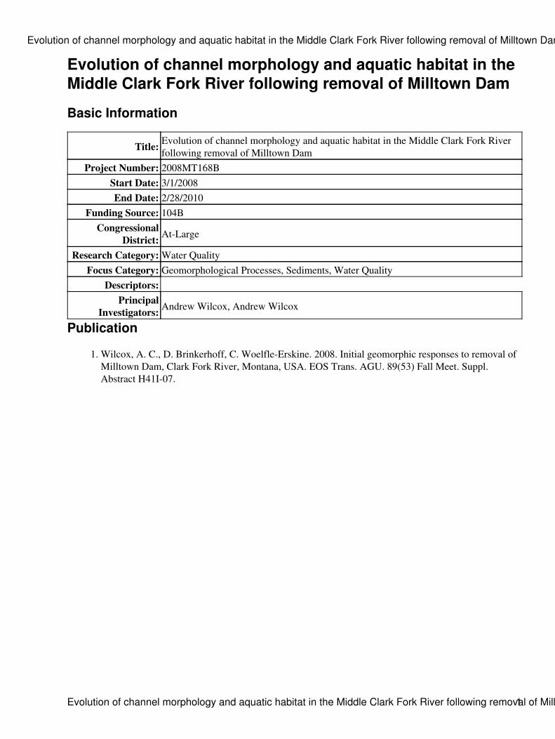
Evolution of channel morphology and aquatic habitat in theMiddle Clark Fork River following removal of Milltown Dam
Basic Information
Title: Evolution of channel morphology and aquatic habitat in the Middle Clark Fork Riverfollowing removal of Milltown Dam
Project Number: 2008MT168BStart Date: 3/1/2008End Date: 2/28/2010
Funding Source: 104BCongressional
District: At-Large
Research Category: Water QualityFocus Category: Geomorphological Processes, Sediments, Water Quality
Descriptors:Principal
Investigators: Andrew Wilcox, Andrew Wilcox
Publication
Wilcox, A. C., D. Brinkerhoff, C. Woelfle-Erskine. 2008. Initial geomorphic responses to removal ofMilltown Dam, Clark Fork River, Montana, USA. EOS Trans. AGU. 89(53) Fall Meet. Suppl.Abstract H41I-07.
1.
Evolution of channel morphology and aquatic habitat in the Middle Clark Fork River following removal of Milltown Dam
Evolution of channel morphology and aquatic habitat in the Middle Clark Fork River following removal of Milltown Dam1

Montana Water Center / USGS Interim report
Evolution of channel morphology and aquatic habitat
in the Middle Clark Fork River following removal of Milltown Dam
Principal Investigator: Andrew Wilcox
Assistant Professor
University of Montana
406-243-4761
We have been investigated geomorphic processes associated with dam removal in the
context of the 2008 removal of Milltown Dam on the Clark Fork River, MT. Funding from the
USGS / Montana Water Center seed grant program has provided an opportunity to conduct time-
sensitive field data collection and analysis, including geomorphic characterization and
geochemical tracer studies, in the months immediately before and after the breach of Milltown
Dam. Our Milltown studies have included:
(1) Documentation of the volume, pattern, and timing of reservoir erosion during the
2008 runoff. This effort combined pre- and post-breach topographic data from Milltown
reservoir and water surface profile measurements throughout the hydrograph that are being used
to reconstruct the spatial and temporal details of sediment evacuation. This effort also entailed
comparison of erosion dynamics in an unconfined reservoir reach (the Clark Fork arm of
Milltown reservoir) versus a confined reservoir reach (the Blackfoot arm of the reservoir). This
analysis documented not only substantial variations in reservoir erosion patterns and mechanisms
(vertical incision versus channel widening) as a function of valley confinement, but also large
variations in the accuracy of sediment transport modeling predictions in these two reservoir
settings.
(2) Collection of bedload transport data during the spring 2008 runoff period, when the
initial downstream sediment pulse moved out of Milltown reservoir.
(3) Development of a preliminary sediment budget for Milltown Reservoir following the
dam breach, combining reservoir erosion estimates (from (1) above), our bedload data, and
USGS suspended flux measurements.
(4) Comparison of measured reservoir erosion and sediment fluxes to predictions based
on HEC-6 modeling by project consultants. This analysis indicated that modeling was reasonably
accurate in the confined BFR arm of Milltown reservoir but had substantial error in the CFR
arm.
(5) Analysis of initial post-removal topographic and textural response upstream and
downstream of Milltown Dam. This effort focused on 2 reaches: the lower 4 km of the Blackfoot
River (BFR) before its confluence with the CFR, and the CFR within 4 km downstream of
Milltown Dam, and entailed pre- and post-breach surveying of 36 cross sections, bed material
sampling, and detailed topographic surveys of lateral and mid-channel bars that we hypothesized
would be locations of active sediment deposition.
(6) Surveying of longitudinal profiles in the lower BFR and in the CFR from Milltown
Dam to 20-km downstream, using a high-resolution, cataraft-based echosounder and GPS
system. These data, combined with qualitative observations collected in the course of these boat-

based surveys about locations of sediment deposition and geomorphic change, are being used to
identify potential transport versus deposition reaches for the next phase of our study.
(7) Sampling and analysis of the size distribution and metals geochemistry of
downstream sediment deposits in order to fingerprint sediment deposits and provide insight into
potential ecosystem effects of contaminated sediment deposition. This effort has included sample
collection extending over 200 km downstream to Thompson Falls, the next downstream
reservoir, at multiple times over the 2008 hydrograph, and measurement of As, Cd, Cu, Zn, Pb,
and Hg concentrations.
(8) Collection and initial analysis of imagery. In summer 2008, high-resolution aerial
photographs were flown from Milltown reservoir to the CFR’s confluence with the Bitterroot
River (paid for by Wilcox startup), and airborne-LIDAR was flown in Milltown reservoir by
contractors to the State of Montana. The LIDAR data have been used as one component of our
analysis of reservoir scour.
(9) Mobilization for data collection, including acquisition of necessary field equipment
for boat-based surveying on a river the size of the CFR (PI’s startup funds), testing and refining
field methods, establishment of field sites, and reconnaissance of additional field sites. Because
of this work we are well positioned for the next phase of field data collection.
Our research has already had impacts in terms of outreach, education, and societal
importance. Three articles featuring this research appeared in the Missoulian. The first of these
appeared on the day of the Milltown Dam breach and detailed our efforts to use the dam removal
to learn about river processes. The second reported on our findings that erosion and downstream
transport of contaminated reservoir sediment had vastly exceeded model predictions and resulted
in widespread downstream deposition. These results heightened public understanding of and
concern about the downstream effects of this dam removal, which had previously received
minimal attention as a result of the focus on the remediation and restoration work upstream of
the dam, in Milltown reservoir. A third article was written by the PI in an effort to clarify our
results. The PI also has spent considerable time discussing our research and results with local
environmental groups (e.g., Clark Fork Coalition, Trout Unlimited, American Whitewater),
citizens, and other media outlets.
Preliminary science outcomes also include a presentation on this research at the Fall 2008
AGU meeting (Wilcox et al. 2008). Two M.S. theses (James Johnsen, Tim Gilbert) partially
supported by the USGS funds will be completed in 2010. The USGS funds have also served as
seed money for a full research proposal submitted earlier this year to the National Science
Foundation, “Sediment routing in gravel-bed rivers following dam removal,” which is pending.
Wilcox, A. C., D. Brinkerhoff, C. Woelfle-Erskine. 2008. “Initial geomorphic responses to
removal of Milltown Dam, Clark Fork River, Montana, USA.” EOS Trans. AGU. 89(53)
Fall Meet. Suppl. Abstract H41I-07.

Student Fellowship: How susceptible to chlorinedisinfection are detached biofilm particles?
Basic Information
Title: Student Fellowship: How susceptible to chlorine disinfection are detached biofilmparticles?
Project Number: 2008MT172BStart Date: 3/1/2008End Date: 12/31/2008
Funding Source: 104BCongressional
District: At-large
Research Category: Biological SciencesFocus Category: Treatment, Toxic Substances, Water Quality
Descriptors:Principal
Investigators: Sabrina Benhke
Publication
Student Fellowship: How susceptible to chlorine disinfection are detached biofilm particles?
Student Fellowship: How susceptible to chlorine disinfection are detached biofilm particles? 1
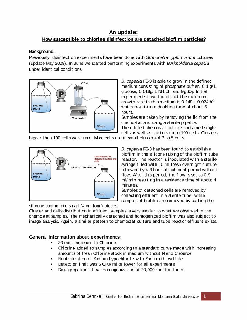
Sabrina Behnke | Center for Biofilm Engineering, Montana State University 1
An update:How susceptible to chlorine disinfection are detached biofilm particles?
Background:Previously, disinfection experiments have been done with Salmonella typhimurium cultures(update May 2008). In June we started performing experiments with Burkholderia cepaciaunder identical conditions.
B. cepacia FS-3 is able to grow in the definedmedium consisting of phosphate buffer, 0.1 g/Lglucose, 0.018g/L NH4Cl, and MgSO4. Initialexperiments have found that the maximumgrowth rate in this medium is 0.148 ± 0.024 h-1
which results in a doubling time of about 6hours.Samples are taken by removing the lid from thechemostat and using a sterile pipette.The diluted chemostat culture contained singlecells as well as clusters up to 100 cells. Clusters
bigger than 100 cells were rare. Most cells are in small clusters of 2 to 5 cells.
B. cepacia FS-3 has been found to establish abiofilm in the silicone tubing of the biofilm tubereactor. The reactor is inoculated with a sterilesyringe filled with 10 ml fresh overnight culturefollowed by a 3 hour attachment period withoutflow. After this period, the flow is set to 0.9ml/min resulting in a residence time of about 4minutes.Samples of detached cells are removed bycollecting effluent in a sterile tube, whilesamples of biofilm are removed by cutting the
silicone tubing into small (4 cm long) pieces.Cluster and cells distribution in effluent samples is very similar to what we observed in thechemostat samples. The mechanically detached and homogenized biofilm was also subject toimage analysis. Again, a similar pattern to chemostat culture and tube reactor effluent exists.
General Information about experiments:• 30 min. exposure to Chlorine• Chlorine added to samples according to a standard curve made with increasing
amounts of fresh Chlorine stock in medium without N and C source• Neutralization of Sodium hypochlorite with Sodium thiosulfate• Detection limit was 5 CFU/ml or lower for all experiments• Disaggregation: shear Homogenization at 20,000 rpm for 1 min.
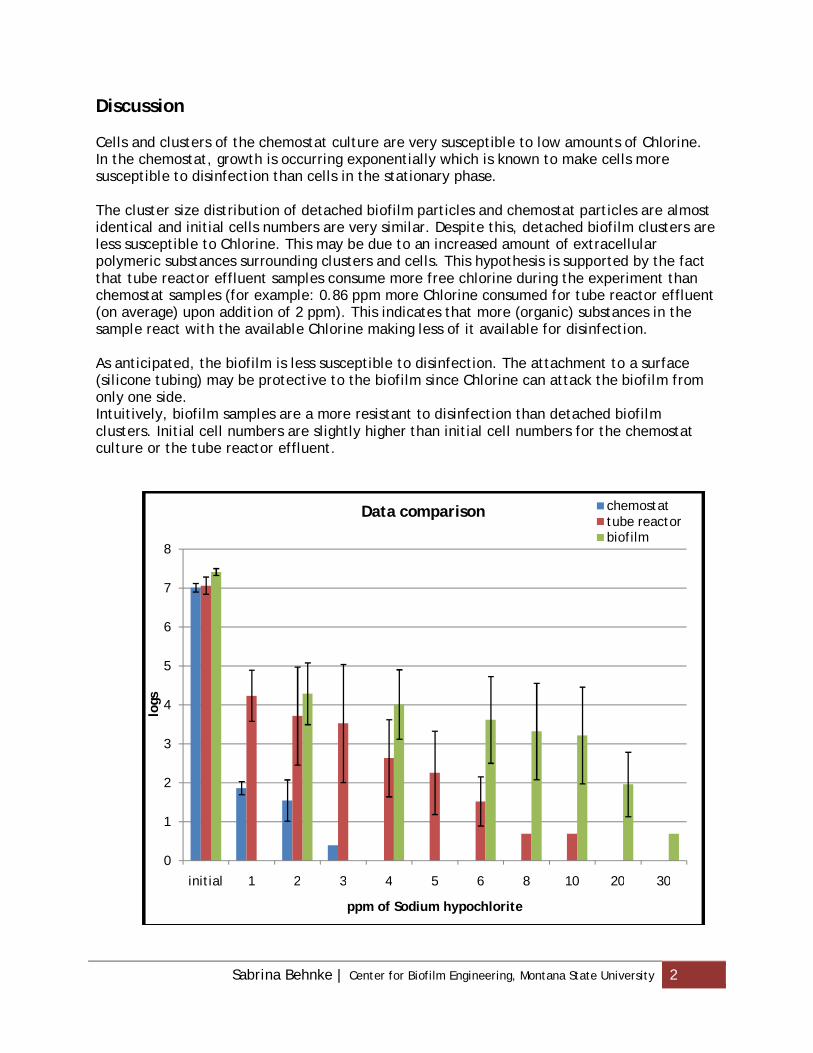
Sabrina Behnke | Center for Biofilm Engineering, Montana State University 2
Discussion
Cells and clusters of the chemostat culture are very susceptible to low amounts of Chlorine.In the chemostat, growth is occurring exponentially which is known to make cells moresusceptible to disinfection than cells in the stationary phase.
The cluster size distribution of detached biofilm particles and chemostat particles are almostidentical and initial cells numbers are very similar. Despite this, detached biofilm clusters areless susceptible to Chlorine. This may be due to an increased amount of extracellularpolymeric substances surrounding clusters and cells. This hypothesis is supported by the factthat tube reactor effluent samples consume more free chlorine during the experiment thanchemostat samples (for example: 0.86 ppm more Chlorine consumed for tube reactor effluent(on average) upon addition of 2 ppm). This indicates that more (organic) substances in thesample react with the available Chlorine making less of it available for disinfection.
As anticipated, the biofilm is less susceptible to disinfection. The attachment to a surface(silicone tubing) may be protective to the biofilm since Chlorine can attack the biofilm fromonly one side.Intuitively, biofilm samples are a more resistant to disinfection than detached biofilmclusters. Initial cell numbers are slightly higher than initial cell numbers for the chemostatculture or the tube reactor effluent.
0
1
2
3
4
5
6
7
8
initial 1 2 3 4 5 6 8 10 20 30
logs
ppm of Sodium hypochlorite
Data comparison chemostattube reactorbiofilm

Student Fellowship: The Consequences of IntrogressiveHybridization: Implications for Westslope Cutthroat TroutConservation
Basic Information
Title: Student Fellowship: The Consequences of Introgressive Hybridization: Implicationsfor Westslope Cutthroat Trout Conservation
Project Number: 2008MT180BStart Date: 3/1/2008End Date: 12/31/2008
Funding Source: 104BCongressional
District: At-large
Research Category: Biological SciencesFocus Category: Ecology, None, None
Descriptors:Principal
Investigators: Matt Corsi
Publication
Student Fellowship: The Consequences of Introgressive Hybridization: Implications for Westslope Cutthroat Trout Conservation
Student Fellowship: The Consequences of Introgressive Hybridization: Implications for Westslope Cutthroat Trout Conservation1

Montana Water Center/USGS Student Fellowship
The Consequences of Introgressive Hybridization: Implications for Westslope
Cutthroat Trout Conservation
by
Matt Corsi
Department of Biological Sciences
University of Montana
Since my last report in June, 2008, I have completed, continued, or begun several
projects. Overall, my dissertation project involves examining the distribution of rainbow and
cutthroat trout hybrid individuals in the Jocko River basin, examining whether individuals with
different hybrid ancestry are different in terms of migration timing, fecundity and growth, as well
as developing a population project model to examine the population implications of different
management scenarios.
In collaboration with Confederated Salish and Kootenai Tribes, I collected fish returning
to spawn and completed collection of fish in tributaries for basin-wide population structure and
hybrid assessment. In late summer and early fall, I obtained genotypes for approximately 500
individual trout in the Jocko River System. In addition, I measured fecundity and removed
otoliths for age and growth estimates. In the coming spring, I will use these genotypes, along
with genotypes collected in previous years, to address migration timing differences between
cutthroat trout, rainbow trout, and their hybrids, as well as to test for differences in fecundity
among the same groups. Finally these genotypes will allow me to complete a fine-scale basin-
wide analysis of the population genetic structure of trout in the Jocko River watershed. Using
this population baseline, I hope to be able to determine with reasonable certainty what breeding
population was the likely source for migratory fish collected during my study. For those fish that
can be reliably assigned to a population, I will examine the relative effects of natal growth
environment and individual level of hybridization on growth rates.
I have begun to develop the population projection model that I will use to evaluate
alternative management strategies for selective passage of migratory cutthroat trout at an
irrigation diversion structure. While this model will eventually include a genetic component to
evaluate the hybridization consequences of allowing migratory rainbow-cutthroat trout to pass the
diversion structure, I have completed the demographic component of the model. The model
suggests, from a purely demographic (not hybridization) standpoint, that passing even a few
migratory individuals above the diversion structure could substantially improve the long-term
population viability of populations upstream of the diversion structure. I presented the results of
this analysis as part of a poster about management of hybrid populations at the American
Fisheries Society 2008 Annual Meeting in Ottawa, Ontario.
The intensive sampling design for fish collection has allowed me to examine both basin-
wide and fine scale spatial structure of the cutthroat and rainbow trout population within the
Jocko River basin. I am beginning an analysis that will address how various spatial sampling
strategies may affect conclusions about hybridization in trout populations. This analysis will
allow managers to better design studies to determine if trout populations are hybridized. These
initial analyses also have spurred a project addressing how sampling approach for population
structure studies have influenced inferences about cutthroat trout life history, genetic migration,
and hybridization. Given that these patterns derive from one hybridized population in the Jocko
River, MT, I am currently working to pull together other data sets of the spatial pattern of
hybridization for westslope cutthroat trout, as well as becoming involved in a project examining
the patterns of hybridization in Snake River cutthroat trout in the Gros Ventre River, WY. Initial
results from samples that I obtained genotypes for this fall indicate a similar landscape pattern to
hybridization as seen in the Jocko River, MT. My project is currently gaining a great deal of
momentum, and I will continue to make substantial gains in the coming year. It is also worth
noting that I completed my comprehensive exams this fall and passed to candidacy in the doctoral
program at the University of Montana.
Student Fellowship: Predictive Modeling of Snowmelt andthe Hydrologic Response:
Basic Information
Title: Student Fellowship: Predictive Modeling of Snowmelt and the HydrologicResponse:
Project Number: 2008MT183BStart Date: 3/1/2008End Date: 11/31/2008
Funding Source: 104BCongressional District: At-large
Research Category: Climate and Hydrologic ProcessesFocus Category: Hydrology, Models, Groundwater
Descriptors:Principal
Investigators: Tyler Smith
Publication
Smith, T. J. and L. A. Marshall (2008). Bayesian methods in hydrologic modeling: A study of recentadvancements in Markov chain Monte Carlo techniques, Water Resources Research, 44, W00B05,doi:10.1029/2007WR006705.
1.
Smith, T. J. 2008. A Conceptual Precipitation-Runoff Modeling Suite: Model Selection, Calibrationand Predictive Uncertainty Assessment. M.S. thesis, Montana State Univ., Bozeman, MT.
2.
Smith, T, L. Marshall. A Bayesian uncertainty framework for conceptual snowmelt and hydrologicmodels applied to the Tenderfoot Creek Experimental Forest. Eos Trans. AGU, 88(52), Fall MeetingSupplement. American Geophysical Union Fall Meeting. 10-14 December 2007. San Francisco, CA.
3.
Student Fellowship: Predictive Modeling of Snowmelt and the Hydrologic Response:
Student Fellowship: Predictive Modeling of Snowmelt and the Hydrologic Response: 1

Montana Water Center/USGS Student Fellowship Final Report
Predictive Modeling of Snowmelt and the Hydrologic Response
by
Tyler Smith Department of Civil Engineering
Montana State University
Because of uncertain mathematical descriptions of the physical hydrologic system,
hydrologists are faced with uncertainty in the prediction of streamflow from a watershed.
This uncertainty is exacerbated in snow-dominated watersheds where the additional
complexity of snowpack simulation must be considered. The research performed in
accordance with the USGS Fellowship project, Predictive Modeling of Snowmelt and the
Hydrologic Response: Tenderfoot Creek Experimental Forest, MT, has been successfully
completed in order to better understand the trade-off between model structural
complexity and predictive performance. In order to quantify this relationship, the project
was divided into four primary research objectives. First, a variety of Markov chain Monte
Carlo techniques, necessary for model parameter estimation and uncertainty analysis
quantification, were explored. Second, a modular modeling framework was established
across a range of structural complexity. An integral component to this objective was to
synthesize the existing observations from the Stringer Creek watershed, located within
Tenderfoot Creek Experimental Forest. Third, the usefulness of alternative data sources for
constraining model predictive uncertainty was investigated. Finally, a self-contained
graphical user interface was developed to integrate the previous objectives into a freely
available modeling software package.
The first objective has successfully resulted in the publication of a paper in a special issue
on model uncertainty analysis in Water Resources Research1, where a series of three
recently developed Markov chain Monte Carlo algorithms necessary to implement model
calibration (parameter estimation) and uncertainty analysis under a Bayesian inferential
approach were implemented and compared in their efficiency and effectiveness. This
objective builds on findings of past studies2, revealing the benefits of newly developed
_____________________________________________________________ 1 Smith, T. J., and L. A. Marshall (2008), Bayesian methods in hydrologic modeling: A study of recent advancements in Markov chain Monte Carlo techniques, Water Resources Research, 44, W00B05, doi:10.1029/2007WR006705. 2 Marshall, L., D. Nott, and A. Sharma (2004), A comparative study of Markov chain Monte Carlo methods for conceptual rainfall-runoff modeling, Water Resources Research, 40, W02501, doi:10.1029/2003WR002378.

methods in better characterizing the full distribution of model parameter values (including
distribution tails) and in more efficiently searching the parameter space. A predictive
modeling framework has been established to analyze the interaction and importance of
model structural complexity and model predictive performance. In doing so, thirty unique
modular structures, ranging in complexity from very simple to moderately complex, have
been developed and included in the modeling suite associated with the modeling
framework. The suite of models was constructed in a modular, component-wise fashion to
address soil moisture accounting and runoff routing, snowmelt accounting, and semi-
distribution of the precipitation inputs to the watershed. This framework then allowed for
the comparison of performance by overall structure and based on individual components.
Each of the models was assessed based on the criteria of performance, uncertainty, and
realism. There was a definite balance between predictive performance and model
complexity with similar performance across a range of structural complexities, indicating
that process description is important to overall simulation of streamflow in conceptual
hydrologic modeling. An alternate data source (snow water equivalents) was used to assess
the realism of internal dynamics of each structure. Finally, a self-contained graphical user
interface was designed to integrate the multiple layers of predictive hydrologic modeling.
The Simulation and Prediction Lab for Analysis of Snowmelt Hydrology (SPLASH) has been
successfully programmed to perform model selection, parameter calibration, uncertainty
analysis, and model evaluation. This software package simplifies the complexities required
to implement a predictive modeling study and shifts the focus toward the modeling
problem itself through the application of forward-looking methods in computational
hydrology.
Dissemination of Findings The research supported by this fellowship has resulted in a published paper in the journal
Water Resources Research, as well as several presentations including the winner of an
outstanding student paper award for the Hydrology Section of the 2007 American
Geophysical Union Fall Meeting. A complete list of the publications and presentations is
listed below.

Smith, T. J. and L. A. Marshall (2008). Bayesian methods in hydrologic modeling: A study of recent advancements in Markov chain Monte Carlo techniques, Water Resources Research, 44, W00B05, doi:10.1029/2007WR006705. Smith, T. J. and L. A. Marshall. 2008. Development and application of a parsimonious snow-hydrologic modeling suite: Investigating the link between model complexity and predictive uncertainty. American Geophysical Union Fall Meeting. 15-19 December 2008. San Francisco, CA. Marshall, L. A. and T. J. Smith. 2008. A study of recently developed MCMC techniques for efficiently characterizing the uncertainty of hydrologic models. American Geophysical Union Fall Meeting. 15-19 December 2008. San Francisco, CA. Smith, T. J. and L. A. Marshall. 2008. A flexible modeling framework for rainfall and snowmelt. American Water Resources Association Montana Section 25th Annual Meeting. 2-3 October 2008. Big Sky, MT. Smith, T. J. and L. A. Marshall. 2008. Advancing Bayesian methods in hydrologic modeling: A study of recently developed Markov chain Monte Carlo techniques. American Statistical Association Montana Chapter Annual Meeting. 16 September 2008. Butte, MT. Smith, T. J. and L. A. Marshall. 2008. A Bayesian uncertainty framework for conceptual snowmelt and hydrologic models applied to the Tenderfoot Creek Experimental Forest. Montana State University Student Research Celebration. 15 April 2008. Bozeman, MT. Smith, T. J. and L. A. Marshall. 2007. A Bayesian uncertainty framework for conceptual snowmelt and hydrologic models applied to the Tenderfoot Creek Experimental Forest. American Geophysical Union Fall Meeting. 10-14 December 2007. San Francisco, CA. Smith, T. J. and L. A. Marshall. 2007. Predictive modeling of snowmelt and the hydrologic response: Tenderfoot Creek Experimental Forest, MT. American Water Resources Association Montana Section 24th
Annual Meeting. 11-12 October 2007. Lewistown, MT.

Information Transfer Program Introduction
Information Transfer Program
The Montana Water Center fills the unique role of coordinating Montana University System (MUS)water-related research, and disseminating and applying its findings for the benefit of the people of the state.And, as Montana is a headwaters state to two of the nation's major river drainage basins: the Missouri and theColumbia, how Montana manages its water and aquatic plants and animals can have far ranging impactsdownstream. Obviously these are not closed systems. Montana's aquatic resources are also impacted by whatcomes into the state, be it acid rain, drought, aquatic nuisance species, or wind carried dust and debris that canincrease snowpack melt. Of course, climate change is a growing concern and, as research is being done todetermine the impact this will have on Montana, the Montana Water Center is part of a multi-disciplinaryeffort to prepare for what seems to be inevitable change. To prepare people need to be informed, and theCenter uses some of its USGS funding to provide forums and outlets for information exchange. During theperiod March 1, 2008 through February 28, 2009, the Montana Water Center drew on its USGS support toconduct programs listed under the Statewide Education and Outreach project.
Information Transfer Program Introduction
Information Transfer Program Introduction 1

Statewide Education and Outreach
Basic Information
Title: Statewide Education and OutreachProject Number: 2008MT187B
Start Date: 3/1/2008End Date: 2/28/2009
Funding Source: 104BCongressional District: At-Large
Research Category: Not ApplicableFocus Category: Hydrology, Surface Water, Groundwater
Descriptors:Principal Investigators: Steve Guettermann
Publication
Whirling Disease Steering Committee of the National Partnership for the Management of Wild andNative Coldwater Fisheries; 2008 Annual Report;http://whirlingdisease.montana.edu/pdfs/2008wdi.pdf (120 pages)
1.
Gretchen Rupp, July 2008 Semi-annual report for the Wildfish Habitat Initiative;http://wildfish.montana.edu/docs/July_2008_semiannual_report.pdf (17 pages)
2.
Statewide Education and Outreach
Statewide Education and Outreach 1

* Worked closely with faculty researchers to engage students in water-related research, writing
papers and professional presentations. In addition, the Water Center encouraged students
engaged in water resource studies to present at conferences. The success of these efforts is
documented by the fact that student involvement with information transfer through the Montana
Water Center rose from approximately two dozen in 2007 to three dozen in 2008.
* Published thirteen Montana Water e-newsletters and distributed them monthly to more than
1,700 professionals, students and decision makers concerned with water resource management; a
special edition was published in March that addressed pharmaceuticals in Montana's water, as a
response to a national study. Newsletter archives are posted at
http://water.montana.edu/newsletter/archives/default.asp.
* In the final stages of a Montana Watersheds Coordination Council website redesign at
http://water.montana.edu/mwcc/default.php - the site is better serving watershed groups
throughout the state, which are also becoming more involved with posting watershed
information.
* Continued the web information network MONTANA WATER, at http://water.montana.edu.
Known as Montana's clearinghouse for water information, this website includes an events page,
news and announcement updates, an online library, water-resource forums and water source
links, a Montana watershed projects database, an expertise directory, water facts and more.
* Completed a project funded by the Montana Department of Environmental Quality to update a
statewide watershed projects database. New projects were added from state agency programs,
federal programs, watershed groups, and NGOs and is now in the process of being turned over to
the Governor's Restoration Initiative program.
* Maintained and circulated a small library of paper documents related to Montana water topics.
* Conducted the state-wide water research meeting on October 2-3, 2008 in Big Sky, Montana.
The theme of this 25th annual meeting was Water Sustainability: Challenges for Montana. It was
held in conjunction with the Montana Section of the American Water Resources Association. A
field trip led by geologist Larry Smith explored the mountainous Big Sky geology and was well
attended. The trip also included the Blue Water Task Force which described how development is
impacted area streams. The conference attracted nearly 150 Montana researchers and policy
makers who took in plenary presentations by Richard Opper, Director of the Montana
Department of Environmental Quality, Eloise Kennedy of the Nature Conservancy, Tom
Osborne, principal of HydroSolutions, Tom Patton, a hydrogeologist at the Montana Bureau of
Mines and Geology and Larry McKay, the GSA Birdsall-Dreiss Distinguished Lecturer for 2008.
Over forty researchers presented information on their latest findings along with nearly 30 poster

displays. The web-based archive of this meeting is found at
http://awra.org/state/montana/events/conf_archives.htm.
* Responded to numerous information requests on water topics ranging from invasive aquatic
species to water rights to streamside setbacks to contaminants and pollutants in Montana's
surface and ground water.
* Assisted elected and appointed officials, particularly those serving on the Montana Legislative
Environmental Quality Council and Water Policy Interim Committee, the Governor's Drought
Advisory Committee and the Water Activities Work Group. The Water Policy Interim
Committee became a standing committee during Montana's 2009 legislative session and the
Water Center expects continued involvement with that group as issues about the state's water and
its use and management become more important and the need to use science and collaboration to
direct policies becomes more accepted.
* Sponsored and participated in Montana's 75th Annual Water School September 22-26, 2008 at
Montana State University for 300 staff members of water and wastewater utilities. This training
covered managing wells and lagoons to process control for water treatment and activated sludge
facilities, treatment plant operation, chemical safety, emergency response, quality assurance
programs, and more; the Montana Water Center was able to get Dr. Robert D. Morris, acclaimed
author of Blue Death, to speak to the public as part of this training.
* Created and distributed 1500 copies of the black-and-white Montana Water 2009 calendar to
elected officials, water resource managers and other partners and supporters; each month features
a different Montana water issue and work agencies and NGOs do to mitigate water-related
management challenges.
* Worked with the Bozeman Film Festival to bring a public showing of the award winning film
FLOW to a local audience, with subsequent post-viewing discussion about the community's
water supply and treatment.
* Worked with the Montana Department of Environmental Quality and the Montana Department
of Transportation to provide professional education to mitigate nonpoint source pollution. The
Montana Watercourse provides comparable outreach to watershed groups, teachers, developers,
and landowners.
* Continued to work with the general public answering questions on water quality, water
quantity, water rights and sustainability issues.

USGS Summer Intern Program
None.
USGS Summer Intern Program 1

Student Support
Category Section 104 BaseGrant
Section 104 NCGPAward
NIWR-USGSInternship
SupplementalAwards Total
Undergraduate 6 0 0 0 6Masters 13 0 0 0 13
Ph.D. 3 0 0 0 3Post-Doc. 0 0 0 0 0
Total 22 0 0 0 22
1

Notable Awards and Achievements
Other work undertaken by the Montana Water Center includes:
The Whirling Disease Initiative - Research is concentrated on understanding how the disease affects troutpopulations, and how management actions may intervene in the process. Dissemination of research and testingresults to fishery managers is also a focus this year.
The goal of the Whirling Disease Initiative and other research enterprises is to develop a clear understandingof the disease cycle, the predisposing environmental factors, and methods for maintaining fisheries despite itspresence. Initiative research has made great strides in the first two areas, and the program is concluding with afocus on assembling, testing and publicizing a toolbox of management methods to support fishery managersas they strive to maintain fisheries in the presence of whirling disease.
Between 1997 and 2006 the Initiative sponsored from six to 20 research projects in each 15-month cycle. Aresearch cycle generally ran from May of one year through December of the following year, allowing for twofield seasons. Broad-scale research investigations begun in May 2006 will conclude at the end of June 2009.One hundred and twenty-four research projects have been carried out by university and public-agencyscientists, and private firms since 1997. More than $5.6 million of federal funds and $4.3 million in matchingfunds have been expended by these research projects. Typically two to four investigators are involved in eachproject, and they bring to the project cash or in-kind match of 25 to 150 percent of the amount of the federalgrant. Students are involved in most projects, either as technicians or, more often, as graduate researchassistants. Summaries of all past and current research projects are available on the Initiative web site at:http://whirlingdisease.montana.edu/.
An interactive map of disease incidence is being mounted on the internet, showing up-to-date information foreight states. Research data from projects funded over the entire course of the initiative are being assembledinto a database that can be used for synoptic studies. Although not a formal Initiative requirement, publicationof research results is strongly encouraged by the Partnership Board and the Steering Committee. To date, atleast 70 peer reviewed publications have been produced.
The Small Systems Technical Assistance Center operated by the Water Center is the flagship of a nationwidenetwork that helps small public water utilities provide safe, reliable and affordable drinking water. This year'sprojects include:
- developing live and electronic training courses on water-system energy efficiency, use of alternative energysources, water loss testing, and water conservation.
- working with the other TACs to develop a more comprehensive website and research and outreach presenceto provide greater nationwide assistance to small public drinking water systems.
The Water Center operates the web site that provides access to the tools developed by all eight technicalassistance centers, and co-sponsors the week-long Montana Water School that draws 250 water treatmentoperators. Its training courses will be presented at a number of national conferences and workshops this year.To date, more than 50,000 water-utility workers have taken the Center's training courses nationwide.
The purpose of the Wild Fish Habitat Initiative is to evaluate the costs and efficacy of measures to bolsterwild fish populations, and publicize the findings among fishery and land managers. A report is submittedsemi-annually to the U.S. Fish & Wildlife Service. The most recent one can be found athttp://wildfish.montana.edu/docs/July_2008_semiannual_report.pdf
Notable Awards and Achievements 1

This year Initiative investigators continue to:
- evaluate the biology of fluvial Arctic grayling to aid restoration efforts in the Big Hole River - test physicaland chemical techniques for eliminating invasive fish species from streams - assess the success of techniquesfor restoration of cutthroat trout in western watersheds - assemble habitat-restoration case histories to assistland managers and fishery biologists in planning new projects.
The Initiative is a scientific adjunct to the Partners for Fish and Wildlife program operated by the U.S. Fishand Wildlife Service for private landowners, aimed to enhance the effectiveness of that program's habitatrestoration projects.
The Montana Watercourse is a statewide program for schools and citizens, providing water information,resources, tools and education. This year's projects include:
- developing and leading water-resource education courses for realtors and teachers - piloting a program ofcertification for volunteer water quality monitors - updating the Landowner's Guide to Montana Wetlands forboth eastern and western Montana - circulating water-resource "teaching trunks" among Montana elementaryschools - completed revision of the Guidebook to Montana Ponds, now in its second printing - operatingKnow-Your-Watershed tours in the Milk and Marias watersheds - organizing the Montana Water Summit forTeachers and Students and received a relatively large grant from Pacific Power & Light in late 2008 for thisspring 2009 event.
Antony Berthelote, as a doctoral student at the University of Montana in the Geosciences Department, wasawarded a trip to the National AWRA Conference in New Orleans by the Montana Section of the AWRA forhis student presentation at the state's water resources conference in Big Sky, Montana, which the MontanaWater Center co-sponsors. The title of his presentation was "Field Observations and Groundwater Modelingas Tools to Mitigate Groundwater Supply Impacts During the Removal of Milltown Dam, Western Montana."Much of Tony's work centers on the impact dam removal can have on the adjacent shallow ground wateraquifers, which has received little study. Tony combines extensive river monitoring, groundwater monitoringand well inventory data with numerical groundwater modeling techniques to forecast areas that wouldexperience groundwater declines.
Notable Awards and Achievements 2