Monoplanar Camera CalibrationIterative Multi-Step Approach

Jorge Batista, Jorge Dias, Helder Araujo, A. Tra^a de AlmeidaInstitute of Systems and Robotics

Department of Electrical Engineering - University ofCoimbraLargo Marques de Pombal-3000 COIMBRA PORTUGAL

Email: jorbat@uc.pt

AbstractA new method for robotics camera calibration based on a linear computation and using a

coplanar group of calibration points is presented in this paper. This new method suppresses the

constraint presented by the RAC calibration model of having an incidence angle between the

optical axis and the calibration plane of at least 30 degrees. The parameters are obtained based on

a multi-step calculation, and the accuracy of the parameters is strongly increased when used on a

iterative calibration. Experimental and simulated analyses results are presented. A comparative

analysis between this new method and the RAC method is presented.

1. IntroductionFrom the mathematical point of view, an image is a projection of a three

dimensional space onto a two dimensional space. Geometric camera calibration is theprocess of determining the 2D-3D mapping between the camera and the worldcoordinate system.

Most of the camera calibration techniques are polarized between approachesclosely related to the classical Photogrammetry approach where accuracy is emphasized,and the approaches geared for automation and robotics, where speed and autonomy areemphasized.

The RAC calibration model presented by R. Tsai [9] [10] was the first cameracalibration model that included radial geometric distortion, uses linear computationmethods and a coplanar group of points for calibration. However, the RAC modelrequires that the angle of incidence between the optical axis and the calibration plane beof at least 30 degrees.

The new method for robotics camera calibration presented in this paper, uses acoplanar group of points, suppressing the constraint of having an incidence angle of atleast 30 degrees required by the RAC model. The computation of the calibrationparameters is linear, and can be decomposed into four steps: (1) rotation matrixcalculation, (2) translation over X and Y axis and horizontal uncertainty scale factorSx, (3) effective focal length, radial distortion coefficient and translation over Z, and (4)image scale factors, image center coordinates and ortoghonality deviation of the imagereferencial axis.

The major contribution for this new method relates with the computation of therotation matrix. The basic principle that leads to the rotation matrix calculation wasfirst presented by Haralick [8] and is based on the fact that there is sufficientinformation on the 2D perspective projection of a rectangle of unknown size in 3Dspace to determine the camera look angle parameters. With the knowledge of therotation matrix, the translation vector and some of the intrinsic parameters can be

BMVC 1993 doi:10.5244/C.7.48

480

obtained using the relationship that defines the same ratio between the image (u",v")and camera (xc,yc) coordinates to obtain the translation in X and Y axis and thehorizontal uncertainty scale factor, followed by the relationship used in the RAC modelto obtain the Z component of the translation vector, and the distortion coefficient k j .The procedure that we use for the computation of the effective focal length/is differentfrom the one presented by Tsai. In this new method we assume an initial value for thefocal length, and we update this value using the Gauss lens law and the perspectivetransformation determined on the plane that includes the line of sight and the opticalaxis of the lens.

With the knowledge of these parameters (Rot,Trans/,k1), the image scale factors,image center coordinates and ortoghonality deviation can be obtained by using theperspective transformation and the transformation between real image coordinates topixels image coordinates.

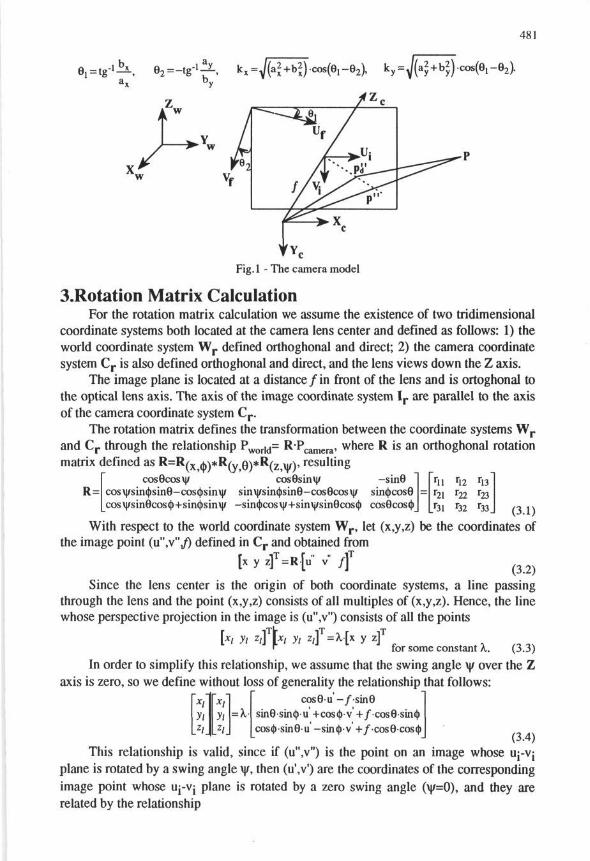
2. Camera ModelIn the following, the underlying camera model (fig. 1) is described briefly, making

note of the parameters that need to be calculated through the calibration procedure.The overall transformation from the 3D object coordinates P(x,y,z) t 0 t n e

computer image frame buffer coordinates p(uf,vj) can be decomposed into thefollowing steps:

1) Rigid body transformation from the object world coordinates to the 3D cameracoordinates system

[xc yc zc] =Rot[x y zf+Trans ^ . l )

where Rot is the rotation matrix and Trans the translation vector.2) Projection from 3D camera coordinate P(xc,yc,zc) to the ideal image coordinate

(u",v ), using perspective projection with pin-hole camera geometry

u" =/••££- v" =/•¥*-zc zc ( 2 2 )

3) Transformation between ideal perspective projection coordinates and real(distorted) perspective projection coordinates, using just one distortion coefficient

Ud Vd ( 2 . 3 )

w h e r e D = l + ( l - 4 k 1 R i d e a l2 ) 1 / 2 , be ing Ri d e a i 2 =u" 2 +v" 2 a n d k j the r ad i a l d i s to r t ion

coefficient.4) Real image coordinate (ud\vd") to computer frame buffer image coordinate

(uf,Vf) transformationuf = axud"+bxvd"+cx v f=ayud"+byvd"+cy ( 2 4 )

where c x and cy represent the image center coordinates (cu,cv) and the remainingparameters relate indirectly to the image scale factors (kx,ky) and the orthogonalitydeviation of the image frame buffer referencial axis (61,62) [6].

Assuming the geometry between the image axis and the frame buffer axispresented in fig 1, the transformation between these coordinate systems can berepresented by

k.cose, •• k-sinG, - -k sin82 ,. kycos62

U f = H ^ T d + H ^ T d +Cu V f = H ^ ) U d + H ^ T d +Cv

being

481

Fig. 1 - The camera model

3.Rotation Matrix CalculationFor the rotation matrix calculation we assume the existence of two tridimensional

coordinate systems both located at the camera lens center and defined as follows: 1) theworld coordinate system W r defined orthoghonal and direct; 2) the camera coordinatesystem C r is also defined orthoghonal and direct, and the lens views down the Z axis.

The image plane is located at a distance/in front of the lens and is ortoghonal tothe optical lens axis. The axis of the image coordinate system I r are parallel to the axisof the camera coordinate system C r .

The rotation matrix defines the transformation between the coordinate systems W r

and C r through the relationship Pworid= R'Pcamera- where R is an orthoghonal rotationmatrix defined as R=R(x,<h)*R(y,6)*R(z,w)' r e s u l t m 8

0 8iR=

cos9cos\|/ cos9sin»j/ —sin9cosv)/sin(|)sin9-cos())sinv|/ sinv|/sin<(>sin9-cos9cosv|/ sin<|)cos9cos\j/sin9cos<])+sin<|)sin\|/ -sin<|)cos\(/+sinysin9cos(j) cos9cos<)> Lr3i '32 '33 J ( 3 1 )

With respect to the world coordinate system W r , let (x,y,z) be the coordinates ofthe image point (u",\"J) defined in C r and obtained from

fx v z]T=Riu" v" f]

Since the lens center is the origin of both coordinate systems, a line passingthrough the lens and the point (x,y,z) consists of all multiples of (x,y,z). Hence, the linewhose perspective projection in the image is (u",v") consists of all the points

[x, y, z,]r[rx, y, y z]

T

for some constant X. (3.3)

In order to simplify this relationship, we assume that the swing angle \|/ over the Zaxis is zero, so we define without loss of generality the relationship that follows:

cos9u —/sin9sin9sin<|)u +cos(|)v'+/cos8sin<()cos<|>-sin9-u'-sin<|>-v'+/-cos9-cos6 „ _v

L J (3.4)This relationship is valid, since if (u",v") is the point on an image whose uj-v;

plane is rotated by a swing angle \|/, then (u',v') are the coordinates of the correspondingimage point whose UJ-VJ plane is rotated by a zero swing angle (y=0), and they arerelated by the relationship

482

|~u'IT cosy sin\|/]ru"][_v'J [-sinv|/ cosyj[v"J (3.5)

The basic observation that leads to the rotation matrix calculation, was firstpresented by Haralick [8] and is based on the fact that there is enough information onthe 2D perspective projection of a rectangle's corners to determine the camera lookangles. Based on this, let us consider the existence of a rectangle of unknown sizelocated perpendicular to the X w axis of the W r coordinate system (fig.2).

Pi/ :

z l/.

x i

°i....

w

If

P3

/

Fig. 2 - Orientation of the rectangle for the rotation matrix calculation

The corners of this rectangle are given byp i=[x i yi zi] p2=[xi y i + w zi] P3=[xi yi Z I+L] P4=[XI yi+w Z I + L ]

where xi>/, and the corresponding perspective projection in the image are.. r .. ..IT „ r .. ,,-iT .. r .. ..-iT „ r .. ,,-iT

Pi =LU1 vlj P2 =LU2 V2j P3 =lu3 V3j P4 =[U4 V4j

Since the pixels coordinates of these points can only be obtained by means of theimage, we need to know in advance the image scale factors and the image centercoordinates. We solve this problem assuming some predefined values for theseparameters, using the same relationships that Tsai uses in the RAC calibration model[9]. We assume an image center located at the center of the image frame buffer (256,256), and scale factors given by the relationships kx=(SxNft)-(dxNcx)"' and ky=dy~

1,where N ^ is the number of frame buffer pixels, N c x is the number of CCD sensors in arow, dx is the distance between CCD sensors in a row, dy that is the distance betweenCCD sensors in a column and finally Sx that represents the horizontal uncertainty scalefactor. We assume in a first stage an unitary uncertainty scale factor.

Let us begin the calculation of the rotation matrix assuming a swing rotation angleequal to zero (y=0), which defines the perspective projection points pj' based on therelationship 3.5. With this assumption, we assume a predefined known swing angle \|/.We also assume a predefined known focal distance/.

Using the relationship 3.4 in order to define the four projective lines of therectangle's corners, we obtain the next matricial equation, which is the basis of thiscomputation.

U| cosB—/sinGUj sin6sin<|)+Vj cos(()+/cos6sin0

•cosbsinG—V: •sin<b+/-cos9-cosd>Jwithi=1..4

The equations 3.5 and 3.6 are sufficient to obtain the three Euler angleswith all the \ i=1 4, and the 3D coordinates of the corners as unknowns.

(3.6)

483

Through the analysis of these matricial relationships, we observe that the first andthird row of equation 3.6 for P t and P2 are identical in order to xj and z j . Conjugatingthese two equations we establish that

/•sin8sin<|>(v2' -v,')+cos6sin<|>(u2 Vj'-ii[ v 2 ^ / c o s ^ U ) - u 2 ) = 0

In an identical manner, the first and third row of equations 3.6 for P3 and P4 areidentical in order to xj and zj+L, which establishes

/•sinesiiKt»(v4'-v3')+cos8sin0(u4 v3 -u3 v4 )+/cos<t>(u3 -u 4 )=0

Multiplying 3.7 by (U3 - 114")and 3.8 by (ui' - 112') and subtracting, results/•sin9-[(v2' -v/)(u3 ' -u4')-(v4' -v3 ')(u/ -u2')]=

=cose[(u4 v 3 -u 3 v ; )^ ; -u 2 ) - (u 2 ' v , ' - u ; v2 ) (u3-u4)]

which by solving for 0 yields

f(u4' v3' -u3' -v^Yu,' -u2')-(u2' v,' -u,' v2')(u3' -u4 ')8=tg~ f •

/ [ ( 2 -v/)(u3 -u4)-(v4 -v3 ).(n,'-u2

The solution for <|> is obtained through the same procedure used for G, multiplyingequation 3.7 by (V4 - V3) and equation 3.8 by (V2 - v\) and subtracting, resulting

[ ]cose[(u2'v1'-u1'v2')(v4'-v3')-(u4 •v3'-u3'-v4)(v2'-v1')]

Observing these last two equations, it is apparent that once \\i is known, then <|> and9 can be solved. The equation that leads to the solution for 9 is not unique, since weobtain a new expression based on the fact that the first and second row of equation 3.6for Pj and P3 are similar in order to xi and yj, and the first and second row of equation3.6 for P2 and P4 are similar in order to xj and yj+W. Using the same procedure asbefore, we obtain an alternate and independent expression for 0, which is

_ l [ ( 2 4 4 2 ) ( i - U 3 ) - ( » 1 V3 - U

- v3 )(u2 - u 4 )-(v2 - v 4 )-(Ul- -

Combining these two expressions for 9 we establish the relationship that togetherwith the equation 3.5 defines the expression that allows the calculation of the last Eulerangle y . Many of the terms included in these equations are \\f rotationally invariant.

Therefore the swing angle \j/ is given by

_ t _,-A(ur-u2")+B-(u3"-U4")+C-(UI"-U3")-D(V2"-V4")

A.(vr-v211)-B-(v3"-v4")-C.(v1--v3")+D.(v2--v4

11) ( J B )

whereA _ u 4 " v 3 " - u 3 " v 4 " _u2"v1"-U|"v2" c = u 2 " v 4 " - u 4 " v 2 " Ul" v3" -u3" V!"

E E F F

E=/[(v2"-v{){»i'-u4")-(v4"-v3")(iii"-u2")] F=/j(v,"-vijnt -u4")-(v2"-v/Xu,"-u3")]

The values obtained for y present an ambiguity of 180 degrees, whereas the valuesfor 9 and $ present an ambiguity of 90 degrees. Values outside this range for the panand tilt angles correspond to the camera looking into the hemisphere behind itself.

484

4. Translation over X and Y and uncertainty scale factor SxUntil now, we assumed that the two coordinate systems W r and C r are located at

the same origin, and that there is no translation between them. This was not a problem,as the computation of the rotation matrix does not require the knowledge of thecoordinates of the rectangle's corners.

Let us now suppose the existence of a translation vector T between both coordinatesystems. Once the rotation matrix is known, points defined in the coordinate system W r

can be converted to the camera coordinate system C r , based on the relationship.^camera=^ot" *\vorid ( w ' t n Rot=RJ). From the ratio between the x and y coordinates of apoint P(xc,yc,zc) defined in C r and its perspective projection u and v coordinates onthe image, we establish the relationship

u"-yc=v"-*c=ud-yc=vxc (4 J)Up to now, we have assumed an unitary uncertainty horizontal scale factor, since

the rotation matrix calculation was not considerably affected by this assumption. This isnot the case for the translation vector. Since we assumed in a first stage a perfect pin-hole camera geometry with a perfectly ortoghonal image and frame buffer coordinatesystems, and the relationship 4.1 remains valid even for image points radially distorted,we obtain the following equation

S ] [Txk I(v f-cx)-Tyky(u f-cy)+Sxkx(v f-cy)X r o t=ky(u f-cx)Y r o t ^ 2 )

by combining equation 4.1 with the referencial relationship P ^ m e ^ R"1. Pworid(with R-1=RT since R is orthogonal) and the relationships uf=Sxkxu"+cx, Vj=kyv"+c ,being Xrot= rn-x+ r21-y+ r31-z, and Yrot= r12-x+ r22-y+ r32-z.

With the knowledge of the uncertainty scale factor, the value assumed in thebeginning for the horizontal scale factor can be updated to be used in the remainingcalculations. If this value obtained for Sx is accurate enough, then its value will be oneif we obtain new values for the rotation matrix and for Tx, Ty and Sx , using theupdated horizontal scale factor. We observed that this conclusion is not valid in the nextiteration, but we converge to it after a few iterations.

It is important to make note that the iterative computation of these calibrationparameters is performed assuming a perfectly orthogonal image and frame buffercoordinate systems. In order to include the computation of this new parameter, newvalues for Tx and T v will be obtained, this time using equations 2.4 combined withequation 4.1, and using the values obtained with the iterative computation for therotation matrix, Tx , Tv and radial distortion coefficient.

5. Translation over Z, Focal length/and Radial distortioncoefficient kj

The basic model that we use in this new methodology for camera calibrationfollows the one presented by Tsai [9], but with a different focal length calculation. Inthat model, in order to integrate the radial distortion, it is assumed the existence of twoconjugate points, one representing the ideal image point projection while the other pointcorresponds to the distorted projection point in the image. The relationship betweenthese points is defined in equations 2.3 of the camera model.

Combining equations 2.3 and the perspective projection relationship yieldsx c /+x c R^/k r u d "T z = ud"zrot y c /+ycRd/k l-vd'T z=vd"-z r o t ( 5 ^

being Rd2=ud"2+vd"2 and z ro t=r13x+r23-y+r33-z.

485

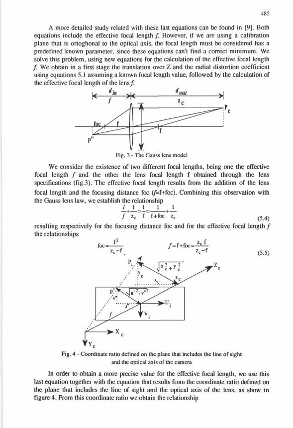
A more detailed study related with these last equations can be found in [9]. Bothequations include the effective focal length /. However, if we are using a calibrationplane that is ortoghonal to the optical axis, the focal length must be considered has apredefined known parameter, since these equations can't find a correct minimum. Wesolve this problem, using new equations for the calculation of the effective focal length/ . We obtain in a first stage the translation over Z and the radial distortion coefficientusing equations 5.1 assuming a known focal length value, followed by the calculation ofthe effective focal length of the lens/.

Fig. 3 - The Gauss lens model

We consider the existence of two different focal lengths, being one the effectivefocal length / and the other the lens focal length f obtained through the lensspecifications (fig.3). The effective focal length results from the addition of the lensfocal length and the focusing distance foe (/=f+foc). Combining this observation withthe Gauss lens law, we establish the relationship

L _L-i-_L_ _L/ zc f f+foc zc ( 5 4 )

resulting respectively for the focusing distance foe and for the effective focal length /the relationships

foc =(5.5)

Fig. 4 - Coordinate ratio defined on the plane that includes the line of sightand the optical axis of the camera

In order to obtain a more precise value for the effective focal length, we use thislast equation together with the equation that results from the coordinate ratio defined onthe plane that includes the line of sight and the optical axis of the lens, as show infigure 4. From this coordinate ratio we obtain the relationship

486

(5.6)that together with the equation 5.5 defines the equations that we use to obtain theeffective focal length/.

6. Scale factors, Image center and Orthogonality deviationof the image referencial axis

We have just described a procedure for the calculation of all the extrinsicparameters as well as some of the intrinsic parameters. This set of parameters togetherwith the parameters whose values were assumed characterize the calibration model.However the values of the parameters calculated are affected by errors due to the factthat the values of the intrinsic parameters were assumed at the beginning.

Based on the knowledge of these parameters and using the relationshipsuf=«Vud"+bx-vd"+Cx v f=ayud"+byvd"+cy ( 6 1 )

we can compute a new solution to the intrinsic parameters ax, ay, b x , b y , c x and cy .The new values calculated for these parameters are much more accurate than the onesinitially assumed.

7. Iterative CalibrationOnce we have calculated more accurate values for the intrinsic parameters

(ax,ay,bx,by,cx,cy.), more accurate calibration parameters can be expected if they areused in an interactive calibration process. Based on that, we can recalibrate, using nowequations 6.1, instead of the relationships of the RAC calibration model.

This iterative procedure is controlled by the accuracy of the image disparity of theprojected calibration points. If the mean value of the image disparity converge to aminimum then the iteration is stopped.

8. Accuracy AnalysisIn order to obtain high accuracy ground truth for the behaviour of this new camera

calibration procedure we simulated the camera calibration setup, taking predefinedvalues for all (he calibration parameters and using these values to obtain noise-freehomologue 2D-3D test and calibration points. Basically, our goal with these simulatedaccuracy analyses is to see how much the values obtained for the calibration parameterswith the calibration process, miss the predefined values from which the calibrationpoints were obtained. We also analized the behaviour of this new method against to thebehaviour of the RAC calibration method, in special, its behaviour with increasingradial distortion and with increasing non-orthogonal image and frame buffer coordinatesystems.

The results obtained with these simulated accuracy analysis are presented ongraphic I on which we can observe that the accuracy of this new method is considerablybetter then the accuracy of the RAC method. However, we observed that this newmethod decreases its performance when the radial distortion increases, while the RACmodel doesn't have its performance considerably change. This results from the fact thatin this new method we assume in the beginning the existence of non radial distortion. Ifthe radial distortion is considerably large, this assumption affects the initial values ofthe iterative process in such a manner, that the convergence of the iterative procedure isnot so good as in the cases of relatively small radial distortion.

487

In the RAC method, if the calibration setup presents an orthogonality deviation ofthe image frame-buffer referencial axis, which results on a calibration points distortionrather than the radial distortion, its performance decreases considerably. This resultsfrom the fact that the RAC model doesn't take into account this type of distortion. Yetfrom the analysis performed with real images, this type of distortion affects thecalibration points, and is one of the reasons why the RAC model presents relativelypoor accuracy when compared with this new method (graph. II).

II

O.OS

O.O+

O.O3

o.ox

O.O1

o

Orthogonal Inalaa

—iMultl—atap 0 ) ...tMurtl-

.—.—IRACBO.OOS <l> tRj

no* gaomatry

-atap 0 0

•vC*>O.OS (II) /

/

aw gaomatry

from tMt to calibration plan* [em} Dlatane* fram tMt to eallbratlon piano

Graph I - Comparative performance analysis between RAC method and Multi-Step method,using simulated images ' \orthogonal geometry: f=25mm, non-orthogonal geometry: f=16mm

(1)*!= -0.000567, e r 8 2 = -0.0627°; (H):k,= -0.000786, 8j-e2= -0.00601°

The behaviour of these two methods is independent of the focal length, and theangle of incidence only affects the performance of the RAC model. As we can see, theaccuracy of the RAC model has better results if the calibration setup presents a non-orthogonal geometry for the optical axis incidence.

Finally, the accuracy of the calibration parameters obtained with this new methodis extremely good, but it's slightly affected for situations of considerably large radialdistortion. In the case of the RAC model, the accuracy of the calibration parameterschanges considerably in the presence of ortoghonality deviation.

In the analysis realized with real images, the performance of this new method wasalways better than the performance of the RAC calibration model, confirming theresults obtained from the simulated analysis. However, we observed that this newmethod is considerably dependant on the accuracy of the corners coordinates of therectangle. This dependence results from the fact that the calculation of the rotationmatrix is done using only the 2D coordinates of the rectangles corners, and nominimum error computation is used. As a result, care must be taken in the selecction ofthe rectangle corners, and with the accuracy of the 2D coordinates of the calibrationpoints.

9. ConclusionA new methodology for robotics camera calibration based on a linear computation

and using a coplanar group of calibration points was presented. The main advantage of

One way of measuring the camera calibration accuracy is to see how much the projective line, that is the raystarting from the lens center passing through the image point, misses the correspondent 3D object point. Theminimum distance between this projective line and the 3D object point is used as an accuracy camera calibrationmeasurement.

488

this new method for camera calibration over the RAC method, is that it doesn'trequire an angle of incidence between the optical axis and the calibration plane over 30degrees, and the uncertainty factor Sx is calculated during the calibration procedure.This method is based on an iterative multi-step approach, and the results obtainedthrough simulated calibrations and real calibrations prove that it is an improvement ofthe RAC method.

11

> from 4**t to •ollbrotlvn plan* [am] Dtstancs from tawt to calibration plans [am]

Graph II - Comparative performance analysis between RAC method andMulti-Step method, using real images in the calibration procedure (f=16mm).

10. References1. H. Martins, J. Birk, R. Kelley, Camera Models Based on Data from Two Calibration Planes,Computer Graphics and Image Processing, vol 17,1981.

2. J. Batista, J. Dias, H. Araujo, A. Trac,a de Almeida, Monoplanar Camera Calibration for Off-the Shelf TV Camera and Lenses - An Iterative Multi-Spet Approach, RecPad93-5l" PortugueseConference of Pattern Recognition, May 13-14, 1993, Porto, Portugal.3. M. Bowman, A. K. Forrest, Transformation Calibration of a Camera Mounted on a Robot,Image and Vision Computing, vol 5, n94, 1987.4. M. Penna, Determining Camera Parameters From The Perspective Projection of aQuadrilateral, Pattern Recognition, vol 24, ns6,1991.5. O. D. Faugeras, G. Toscani, The Calibration Problem for Stereoscopic Vision, Nato ASISeries, Vol. F52,1989.6. R. Kelley, Calibrage des Cameras Video. Application a l'etude de la derive temporale d'unecamera, Rapport de Recherch n2 83.006, LAAS, Toulose, 1983.7. R. Haralick, Using Perspective Transformation in Scene Analysis, CGIP, 13,1980.8. R. Haralick, Determining Camera Parameters from the Perspective Projection of a Rectangle,Pattern Recognition, vol 22, n93, 1989.9. R. Y. Tsai, A Versatile Camera Calibration Technique for High-Accuracy 3D Machine VisionMetrology Using Off-the Shelf TV cameras and Lenses, IEEE Journal of Robotics andAutomation, vol.RA-3, Ns 4, August 1987.10. R. Y. Tsai, R. K. Lenz, Review of RAC-Based Camera Calibration, Vision, vol 5, n93.11. T. Echigo, A Camera Calibration Technique using TTiree Sets of Parallel Lines, MachineVision and Applications, vol 3, pg 159-167,1990.12. W. Chen, B. Jiang, 3D Camera Calibration Using Vanishing Points Concept, PatternRecognition, vol 24, n9 1,1991.