Brown Computer Science Technical Report, TR-CS-02-04

Monitoring Streams – A New Class of Data Management Applications

Don Carney Brown University

dpc@cs.brown.edu

Ugur Cetintemel Brown University

ugur@cs.brown.edu

Mitch Cherniack Brandeis University

mfc@cs.brandeis.edu

Christian Convey Brown University cjc@cs.brown.edu

Sangdon Lee

Brown University sdlee@cs.brown.edu

Greg Seidman Brown University gss@cs.brown.edu

Michael Stonebraker

M.I.T. stonebraker@lcs.mit.edu

Nesime Tatbul Brown University

tatbul@cs.brown.edu

Stan Zdonik

Brown University sbz@cs.brown.edu

Abstract This paper introduces monitoring applications, which we will show differ substantially from conventional business data processing. The fact that a software system must process and react to continual inputs from many sources (e.g., sensors) rather than from human operators requires one to rethink the fundamental architecture of a DBMS for this application area. In this paper, we present Aurora, a new DBMS that is currently under construction at Brandeis University, Brown University, and M.I.T. We describe the basic system architecture, a stream-oriented set of operators, optimization tactics, and support for real-time operation.

1 Introduction Traditional DBMSs have been oriented toward business data processing, and consequently are designed to address the needs of these applications. First, they have assumed that the DBMS is a passive repository storing a large collection of data elements and that humans initiate queries and transactions on this repository. We call this a Human-Active, DBMS-Passive (HADP) model. Second, they have assumed that the current state of the data is the only thing that is important. Hence, current values of data elements are easy to obtain, while previous values can only be found torturously by decoding the DBMS log. The third assumption is that triggers and alerters are second-class citizens. These constructs have been added as an after thought to current systems, and none have an implementation that scales to a large number of triggers. In addition, there is typically little or no support for querying a “trigger base.” Fourth, DBMSs assume that data elements have precise values (e.g., employee salaries), and have little or no support for data elements that are imprecise or out-of-date. Lastly, DBMSs assume that applications require no real-time services.

There is a substantial class of applications where all five assumptions are problematic. Monitoring applications are applications that monitor continuous streams of data. This

class of applications includes military applications that monitor readings from sensors worn by soldiers (e.g., blood pressure, heart rate, position), financial analysis applications that monitor streams of stock data reported from various stock exchanges, and tracking applications that monitor the locations of large numbers of objects for which they are responsible (e.g., audio-visual departments that must monitor the location of borrowed equipment). Because of the high volume of monitored data and the query requirements for these applications, monitoring applications would benefit from DBMS support. Existing DBMS systems, however, are ill suited for such applications since they target business applications.

First, monitoring applications get their data from external sources (e.g., sensors) rather than from humans issuing transactions. The role of the DBMS in this context is to alert humans when abnormal activity is detected. This is a DBMS-Active, Human-Passive (DAHP) model.

Second, monitoring applications require data management extending over the entire history of values reported in a stream, and not just over the most recently reported values. Consider a monitoring application that tracks the location of items of interest, such as overhead transparency projectors and laptop computers, using electronic property stickers attached to the objects. Ceiling-mounted sensors inside a building and the GPS system in the open air generate large volumes of location data. If a reserved overhead projector is not in its proper location, then one might want to know the geographic position of the missing projector. In this case, the last value of the monitored object is required. However, an administrator might also want to know the duty cycle of the projector, thereby requiring access to the entire historical time series.

Third, most monitoring applications are trigger-oriented. If one is monitoring a chemical plant, then one wants to alert an operator if a sensor value gets too high or if another sensor value has recorded a value out of range more than twice in the last 24 hours. Every application could potentially monitor multiple streams of data, requesting alerts if complicated conditions are met. Thus, the scale of trigger processing required in this environment far exceeds that found in traditional DBMS applications.

0

Fourth, stream data is often lost, stale, or imprecise. An object being monitored may move out of range of a sensor system, thereby resulting in lost data. The most recent report on the location of the object becomes more and more inaccurate over time. Moreover, sensors that record bodily functions (such as heartbeat) are quite imprecise, and have margins of error that are significant in size.

Input data streams

Output to applications

Continuous & ad hocqueries

Operator boxes HistoricalStorage

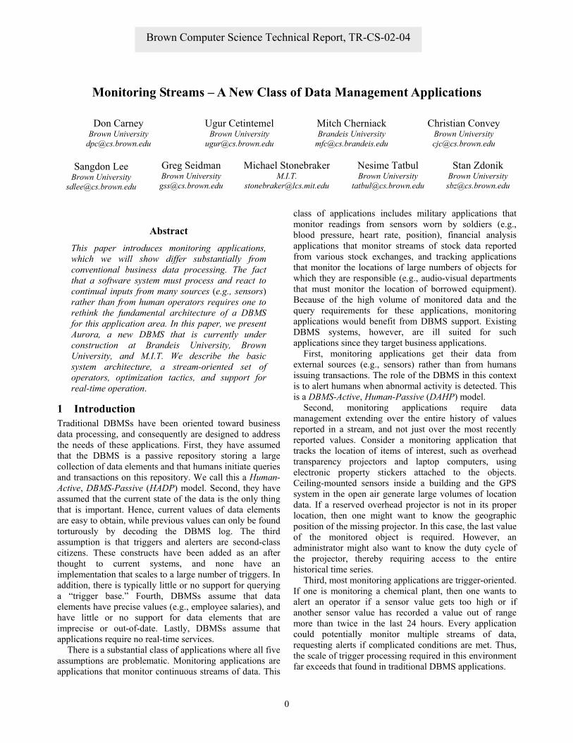
Figure 1: Aurora system model

Lastly, many monitoring applications have real-time requirements. Applications that monitor mobile sensors (e.g., military applications monitoring soldier locations) often have a low tolerance for stale data, making these applications effectively real time. The added stress on a DBMS that must serve real-time applications makes it imperative that the DBMS employ intelligent resource management (e.g., scheduling) and graceful degradation strategies (e.g., load shedding) during periods of high load.

Monitoring applications are very difficult to implement in traditional DBMSs. First, the basic computation model is wrong: DBMSs have a HADP model while monitoring applications often require a DAHP model. In addition, to store time-series information one has only two choices. First, he can encode the time series as current data in normal tables. In this case, assembling the historical time series is very expensive because the required data is spread over many tuples, thereby dramatically slowing performance. Alternately, he can encode time series information in binary large objects (BLOBs) to achieve physical locality, at the expense of making queries to individual values in the time series very difficult. The only system that we are aware of that tries to do something more intelligent with time series data is the Informix Universal Server, which implemented a time-series data type and associated methods that speed retrieval of values in a time series [1].

If a monitoring application had a very large number of triggers or alerters, then current DBMSs would fail because they do not scale past a few triggers per table. The only alternative is to encode triggers in some middleware application. Using this implementation, the system cannot reason about the triggers (e.g., optimization), nor can the triggers be queried because they are outside the DBMS. Moreover, performance is typically poor because middleware must poll for data values that triggers and alerters depend on.

Lastly, no DBMS that we are aware of has built-in facilities for imprecise or stale data. The same comment applies to real-time capabilities. Again, the user must build custom code into his application.

For these reasons, monitoring applications are difficult to implement using traditional DBMS technology. To do better, all the basic mechanisms in current DBMSs must be rethought. In this paper, we describe a prototype system, Aurora, which is designed to better support monitoring applications. We use Aurora to illustrate design issues that would arise in any system of this kind.

Monitoring applications are applications for which streams of information, triggers, imprecise data, and real-time requirements are prevalent. We expect that there will

be a large class of such applications. For example, we expect the class of monitoring applications for physical facilities (e.g., monitoring unusual events at nuclear power plants) to grow in response to growing needs for security). In addition, as GPS-style devices are attached to a broader and broader class of objects, monitoring applications will expand in scope. Currently such monitoring is expensive and is restricted to costly items like automobiles (e.g., Lojack technology). In the future, it will be available for most objects whose position is of interest.

In Section 2, we begin by describing the basic Aurora architecture and fundamental building blocks. In Section 3, we show why traditional query optimization fails in our environment, and present our alternate strategies for optimizing Aurora applications. Section 4 describes the run-time architecture and behavior of Aurora, concentrating on storage organization, scheduling, introspection, and load shedding. In Section 5, we discuss the myriad of related work that has preceded our effort. Finally, we conclude in Section 6.

2 Aurora System Model Aurora data is assumed to come from a variety of data sources such as computer programs that generate values at regular or irregular intervals or hardware sensors. We will use the term data source for either case. In addition, a data stream is the term we will use for the collection of data values that are presented by a data source. Each data source is assumed to have a unique source identifier and Aurora timestamps every incoming tuple to monitor the quality of service being provided.

The basic job of Aurora is to process incoming streams in the way defined by an application administrator. Aurora is fundamentally a data-flow system and uses the popular boxes and arrows paradigm found in most process flow and workflow systems. Hence, tuples flow through a loop-free, directed, graph of processing operations (i.e., boxes). Ultimately, output streams are presented to applications, which must be programmed to deal with the asynchronous tuples in an output stream. Aurora can also maintain historical storage, primarily in order to support ad-hoc queries. Figure 1 illustrates the high-level system model.

Aurora Operators. Aurora contains built-in support for seven primitive operations for expressing its stream processing requirements. The filter box applies a predicate to each incoming tuple, passing only the ones that satisfy

1

the predicate. Merge combines two streams of data into a single stream. Resample is a powerful operation that predicts additional values that are not originally contained in a stream. This operation can be used to create new values in the stream by interpolating between existing values. In addition, Aurora provides a drop box that removes tuples from the stream, and is used primarily to shed load when Aurora is not providing reasonable service (see Section 4.5). Join is a windowed version of the standard relational join. Join pairs elements in separate streams whose distance (e.g., difference in time, relative position, etc.) is within a specified bound. This bound is considered the size of the window for the join. For example, the window might be 30 minutes if one wanted to pair all securities that had the same price within a half hour of each other. In environments where data can be stale or time imprecise, windowed operations are a necessity. The last box is called map and it supports the application of a (user-defined) function to every element of a data stream. Some functions just transform individual items in the stream to other items, while others, such as moving average, apply a function across a window of values in a stream. Hence, map has both a windowed and non-windowed version. A precise definition for each of these operators is contained in Appendix 1.

O1

O4

O3O2

O5 O6

continuous queryview

QOS spec

Persistence spec:“Keep 1 hr”

appstorage

O7 O8 O9

Connectionpoint

ad-hoc query

storage

app

Persistence spec:“Keep 2 hr”

S1 S2

S3

QOS spec

QOS spec

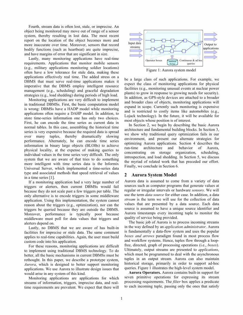
Figure 2: Aurora query model

There are no condition boxes in an Aurora network. Instead, an application would have to include two filter boxes providing both the condition and the converse of the condition. At some inconvenience to an application, this results in a simpler system structure. Additionally, there is no explicit split box; instead, the application administrator can connect the output of one box to the input of several others. This implements an implicit split operation. On the other hand, there is an explicit Aurora merge operation, whereby two streams can be put together. If, additionally, one tuple must be delayed for the arrival of a second one, then a resample box can be inserted in the Aurora network to accomplish this effect.

Aurora Query Model. Aurora supports continual queries (real-time processing), views, and ad-hoc queries all using substantially the same mechanisms. All three modes of operation use the same conceptual building blocks. Each mode processes information flows based on QoS specificationseach output in Aurora is associated with two-dimensional QoS graphs that specify the utility of the output in terms of several performance and quality related attributes (see Section 4.1). The diagram in Figure 2 illustrates the processing modes supported by Aurora.

The topmost path represents a continuous query. In isolation, data elements flow into boxes, are processed, and flow further downstream. In this scenario, there is no need to store any data elements once they are processed. Once an input has worked its way through all reachable paths, that data item is drained from the network. The QoS specification at the end of the path controls how resources are allocated to the processing elements along the path. One can also view an Aurora network (along with some of its applications) as a large collection of triggers. Each path

from a sensor input to an output can be viewed as computing the condition part of a complex trigger. An output tuple is delivered to an application, which can take the appropriate action.

The dark circles on the input arcs to boxes O1 and O2 represent connection points. A connection point is an arc that will support dynamic modification to the network. New boxes can be added to or deleted from a connection point. When a new application connects to the network, it will often require access to the recent past. As such, a connection point has the potential for persistent storage (see Section 4.2). Persistent storage retains data items beyond their processing by a particular box. In other words, as items flow past a connection point, they are cached in a persistent store for some period of time. They are not drained from the network by applications. Instead, a persistence specification indicates exactly how long the items are kept. In the figure, the left-most connection point is specified to be available for two hours. This indicates the beginning of time for newly connected applications will be two hours in the past.

The middle path in Figure 2 represents a view. In this case, a path is defined with no connected application. It is allowed to have a QoS specification as an indication of the importance of the view. Applications can connect to the end of this path whenever there is a need. Before this happens, the system can propagate some, all, or none of the values stored at the connection point in order to reduce latency for applications that connect later. Moreover, it can store these partial results at any point along a view path. This is analogous to a materialized or partially materialized view. View materialization is under the control of the scheduler.

The bottom path represents an ad-hoc query. An ad-hoc query can be attached to a connection point at any time. The semantics of an ad-hoc query is that the system will process data items and deliver answers from the earliest time T (persistence spec.) stored in the connection point until the query branch is explicitly disconnected. Thus, the semantics for an Aurora ad-hoc query is the same as a continuous query that starts executing at tnow− T and continues until explicit termination.

Aurora User Interface. The Aurora user interface cannot be covered in detail because of space limitations.

2

Here, we mention only a few salient features. To facilitate designing large networks, Aurora will support a hierarchical collection of groups of boxes. A designer can begin near the top of the hierarchy where only a few superboxes are visible on the screen. A zoom capability is provided to allow him to move into specific portions of the network, by replacing a group with its constituent boxes and groups. In this way, a browsing capability is provided for the Aurora diagram.

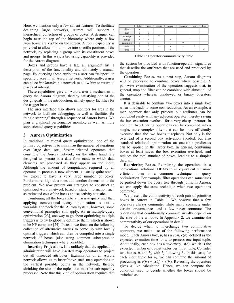
filter map w. map merge resample join drop filter + map ? ?

w. map - ? ? merge + + - +

resample ? ? - - ? join ? ? - - - ? drop + + - + - - +

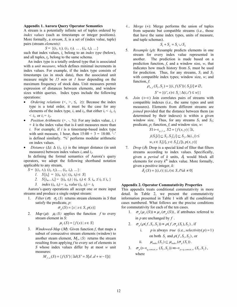
Table 1: Operator commutativity table

Boxes and groups have a tag, an argument list, a description of the functionality and ultimately a manual page. By querying these attributes a user can “teleport” to specific places in an Aurora network. Additionally, a user can place bookmarks in a network to allow him to return to places of interest.

These capabilities give an Aurora user a mechanism to query the Aurora diagram, thereby satisfying one of the design goals in the introduction, namely query facilities for the trigger base.

The user interface also allows monitors for arcs in the network to facilitate debugging, as well as facilities for “single stepping” through a sequence of Aurora boxes. We plan a graphical performance monitor, as well as more sophisticated query capabilities.

3 Aurora Optimization In traditional relational query optimization, one of the primary objectives is to minimize the number of iterations over large data sets. Stream-oriented operators that constitute the Aurora network, on the other hand, are designed to operate in a data flow mode in which data elements are processed as they appear on the input. Although the amount of computation required by an operator to process a new element is usually quite small, we expect to have a very large number of boxes. Furthermore, high data rates add another dimension to the problem. We now present our strategies to construct an optimized Aurora network based on static information such as estimated cost of the boxes and selectivity statistics.

Combining all the boxes into a massive query and then applying conventional query optimization is not a workable approach for the Aurora system; however, some conventional principles still apply. As in multiple-query optimization [23], one way to go about optimizing multiple triggers is to try to globally optimize them, which is shown to be NP-complete [24]. Instead, we focus on the following collection of alternative tactics to come up with locally optimal triggers which can then be compiled into a single network of boxes (also using common subexpression elimination techniques where possible).

Inserting Projections. It is unlikely that the application administrator will have inserted map operators to project out all unneeded attributes. Examination of an Aurora network allows us to insert/move such map operations to the earliest possible points in the network, thereby shrinking the size of the tuples that must be subsequently processed. Note that this kind of optimization requires that

the system be provided with function/operator signatures that describe the attributes that are used and produced by the operators.

Combining Boxes. As a next step, Aurora diagrams will be processed to combine boxes where possible. A pair-wise examination of the operators suggests that, in general, map and filter can be combined with almost all of the operators whereas windowed or binary operators cannot.

It is desirable to combine two boxes into a single box when this leads to some cost reduction. As an example, a map operator that only projects out attributes can be combined easily with any adjacent operator, thereby saving the box execution overhead for a very cheap operator. In addition, two filtering operations can be combined into a single, more complex filter that can be more efficiently executed than the two boxes it replaces. Not only is the overhead of a second box activation avoided, but also standard relational optimization on one-table predicates can be applied in the larger box. In general, combining boxes at least saves the box execution overhead, and reduces the total number of boxes, leading to a simpler diagram.

Reordering Boxes. Reordering the operations in a conventional relational DBMS to an equivalent but more efficient form is a common technique in query optimization. For example, filter operations can sometimes be pushed down the query tree through joins. In Aurora, we can apply the same technique when two operations commute.

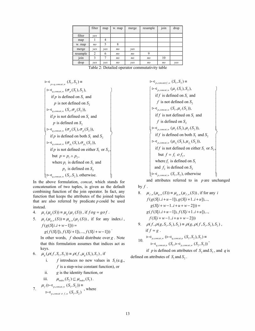
We present the commutativity of each pair of primitive boxes in Aurora in Table 1. We observe that a few operators always commute, while many commute under certain circumstances and a few never commute. The operations that conditionally commute usually depend on the size of the window. In Appendix 2, we examine the commutativity of our operations in detail.

To decide when to interchange two commutative operators, we make use of the following performance model. Each Aurora box, b, has a cost, c(b), defined as the expected execution time for b to process one input tuple. Additionally, each box has a selectivity, s(b), which is the expected number of output tuples per input tuple. Consider two boxes, bi and bj, with bj following bi. In this case, for each input tuple for bi, we can compute the amount of processing as c(bi) + c(bj) × s(bi). Reversing the operators gives a like calculation. Hence, we can compute the condition used to decide whether the boxes should be switched as:

3

1 ( ) / ( ) 1 ( ) / ( ij j i )s b c b s b c b− > −

It is straightforward to generalize the above calculation to deal with cases that involve fan-in or fan-out situations. Moreover, it is easy to see that we can obtain an optimal ordering by sorting all the boxes according to their corresponding ratios in decreasing order. We use this result in a heuristic algorithm that iteratively reorders boxes (to the extent allowed by their commutativity properties) until no more reorderings are possible.

Ad-Hoc Query Optimization. Recall that the semantics of an ad-hoc query is that it must run on all the historical information saved at the connection point(s) to which it is connected. Subsequently, it becomes a normal portion of an Aurora network, until it is discarded.

Aurora processes ad-hoc queries in two steps. First, it runs the portion of the query that uses the historical information in the connection point. The storage system is free to organize this storage in any way that it deems appropriate (e.g., a B-tree). When this finishes, it switches to normal operation on the queue data structures (see Section 4.2). To optimize historical queries, Aurora begins at each connection point and examines the successor box(es). If the box is a filter, then Aurora examines the condition to see if it is compatible with the storage key associated with the connection point. If so, it switches the implementation of the filter box to perform an indexed lookup in the B-tree. Similarly, if the successor box is a join, then Aurora costs performing a merge-sort or indexed lookup, chooses the cheapest one, and changes the join implementation appropriately. Other boxes cannot effectively use the indexed structure, so only these two need be considered. Moreover, once the initial box performs its work on the historical tuples, the index structure is lost, and all subsequent boxes will work in the normal way.

Hence, the initial boxes in an ad-hoc query can “pull” information from the B-tree associated with the corresponding connection point(s). After that, the normal “push” processing associated with Aurora operation takes over. When, the historical operation is finished, Aurora

switches the implementation to the queued data structures, and continues processing in the conventional fashion.

…Q1

…Q2...

…Qi

Buffer manager

…Qj

…Qn

.

.

.

StorageManager

Persistent Store

Scheduler

Router

Catalogs

σ

µ...

Box Processors

inputs outputs

LoadShedder

QoSMonitor

><

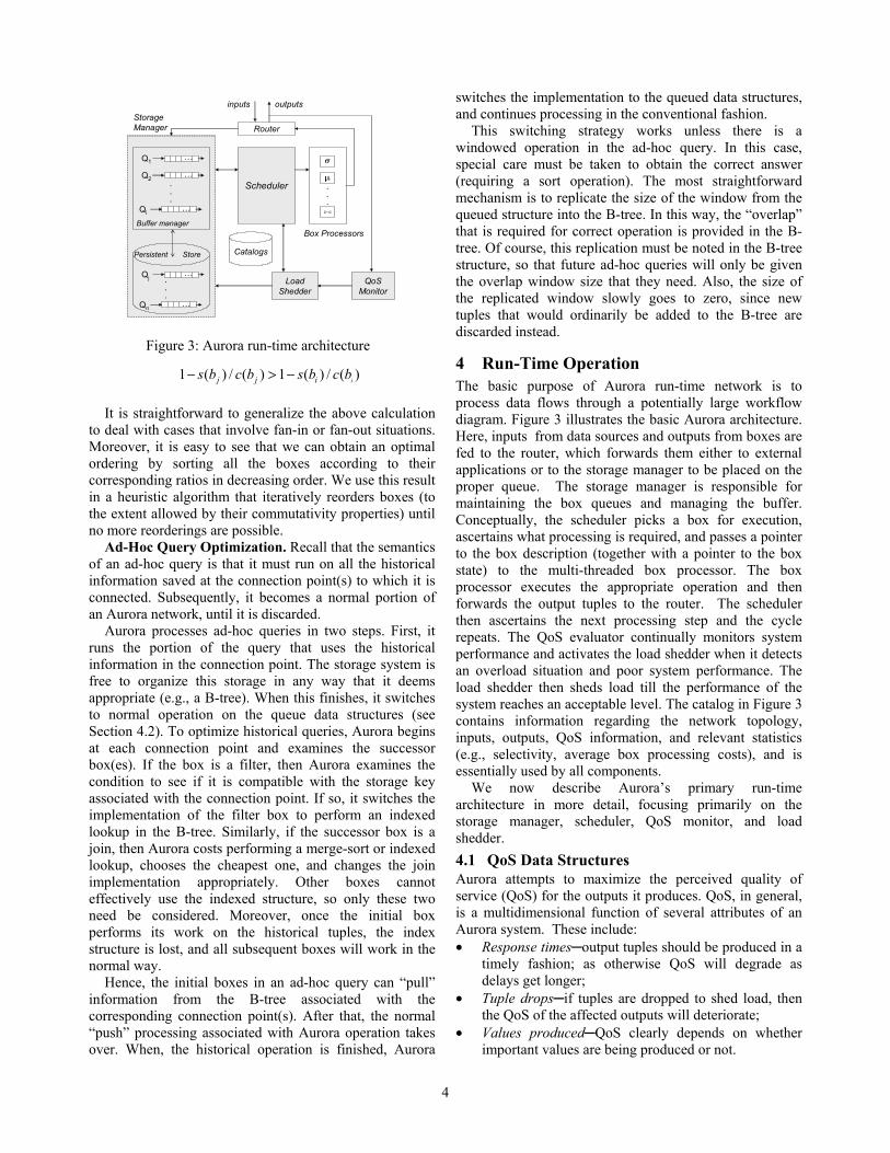
Figure 3: Aurora run-time architecture

This switching strategy works unless there is a windowed operation in the ad-hoc query. In this case, special care must be taken to obtain the correct answer (requiring a sort operation). The most straightforward mechanism is to replicate the size of the window from the queued structure into the B-tree. In this way, the “overlap” that is required for correct operation is provided in the B-tree. Of course, this replication must be noted in the B-tree structure, so that future ad-hoc queries will only be given the overlap window size that they need. Also, the size of the replicated window slowly goes to zero, since new tuples that would ordinarily be added to the B-tree are discarded instead.

4 Run-Time Operation The basic purpose of Aurora run-time network is to process data flows through a potentially large workflow diagram. Figure 3 illustrates the basic Aurora architecture. Here, inputs from data sources and outputs from boxes are fed to the router, which forwards them either to external applications or to the storage manager to be placed on the proper queue. The storage manager is responsible for maintaining the box queues and managing the buffer. Conceptually, the scheduler picks a box for execution, ascertains what processing is required, and passes a pointer to the box description (together with a pointer to the box state) to the multi-threaded box processor. The box processor executes the appropriate operation and then forwards the output tuples to the router. The scheduler then ascertains the next processing step and the cycle repeats. The QoS evaluator continually monitors system performance and activates the load shedder when it detects an overload situation and poor system performance. The load shedder then sheds load till the performance of the system reaches an acceptable level. The catalog in Figure 3 contains information regarding the network topology, inputs, outputs, QoS information, and relevant statistics (e.g., selectivity, average box processing costs), and is essentially used by all components.

We now describe Aurora’s primary run-time architecture in more detail, focusing primarily on the storage manager, scheduler, QoS monitor, and load shedder. 4.1 QoS Data Structures Aurora attempts to maximize the perceived quality of service (QoS) for the outputs it produces. QoS, in general, is a multidimensional function of several attributes of an Aurora system. These include: • Response times─output tuples should be produced in a

timely fashion; as otherwise QoS will degrade as delays get longer;

• Tuple drops─if tuples are dropped to shed load, then the QoS of the affected outputs will deteriorate;

• Values produced─QoS clearly depends on whether important values are being produced or not.

4

QoS

% tuples delivered

1

0

100 0

QoS

delay

1

0

δ

good zone

QoS

output value

1

0

(a) drop-based (b) delay-based (c) value-based

Figure 4: QoS graph types

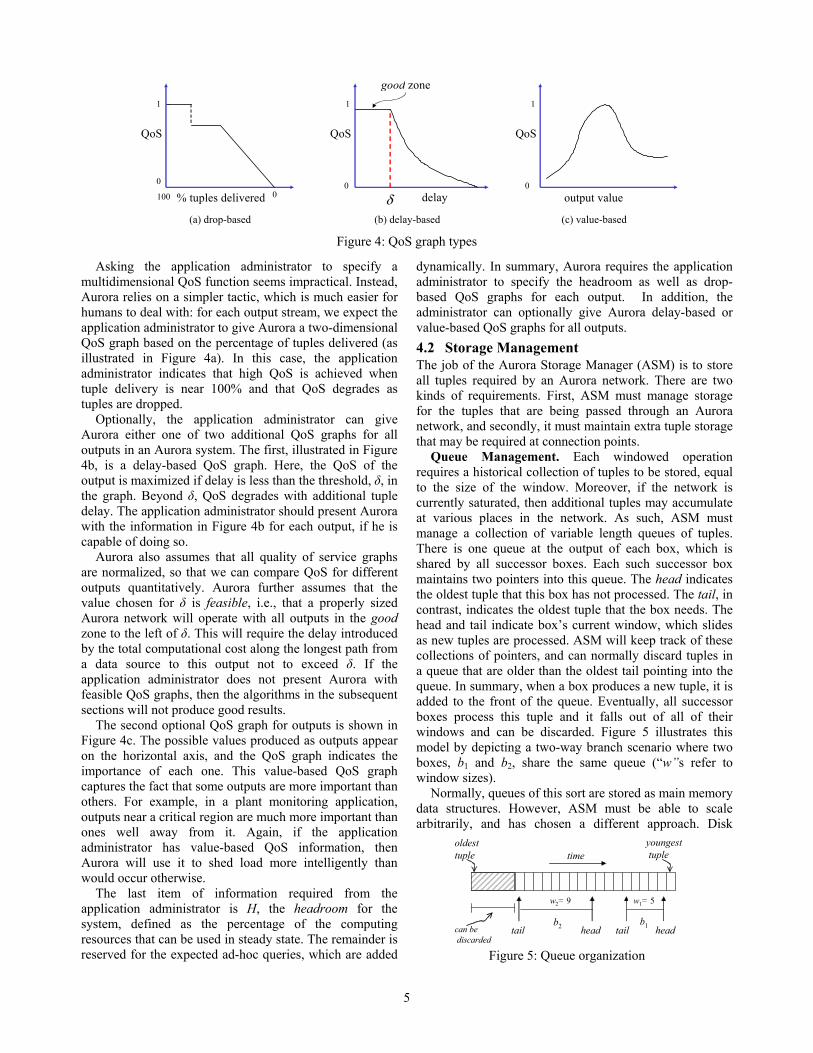
Asking the application administrator to specify a multidimensional QoS function seems impractical. Instead, Aurora relies on a simpler tactic, which is much easier for humans to deal with: for each output stream, we expect the application administrator to give Aurora a two-dimensional QoS graph based on the percentage of tuples delivered (as illustrated in Figure 4a). In this case, the application administrator indicates that high QoS is achieved when tuple delivery is near 100% and that QoS degrades as tuples are dropped.

Optionally, the application administrator can give Aurora either one of two additional QoS graphs for all outputs in an Aurora system. The first, illustrated in Figure 4b, is a delay-based QoS graph. Here, the QoS of the output is maximized if delay is less than the threshold, δ, in the graph. Beyond δ, QoS degrades with additional tuple delay. The application administrator should present Aurora with the information in Figure 4b for each output, if he is capable of doing so.

Aurora also assumes that all quality of service graphs are normalized, so that we can compare QoS for different outputs quantitatively. Aurora further assumes that the value chosen for δ is feasible, i.e., that a properly sized Aurora network will operate with all outputs in the good zone to the left of δ. This will require the delay introduced by the total computational cost along the longest path from a data source to this output not to exceed δ. If the application administrator does not present Aurora with feasible QoS graphs, then the algorithms in the subsequent sections will not produce good results.

The second optional QoS graph for outputs is shown in Figure 4c. The possible values produced as outputs appear on the horizontal axis, and the QoS graph indicates the importance of each one. This value-based QoS graph captures the fact that some outputs are more important than others. For example, in a plant monitoring application, outputs near a critical region are much more important than ones well away from it. Again, if the application administrator has value-based QoS information, then Aurora will use it to shed load more intelligently than would occur otherwise.

The last item of information required from the application administrator is H, the headroom for the system, defined as the percentage of the computing resources that can be used in steady state. The remainder is reserved for the expected ad-hoc queries, which are added

dynamically. In summary, Aurora requires the application administrator to specify the headroom as well as drop-based QoS graphs for each output. In addition, the administrator can optionally give Aurora delay-based or value-based QoS graphs for all outputs. 4.2 Storage Management The job of the Aurora Storage Manager (ASM) is to store all tuples required by an Aurora network. There are two kinds of requirements. First, ASM must manage storage for the tuples that are being passed through an Aurora network, and secondly, it must maintain extra tuple storage that may be required at connection points.

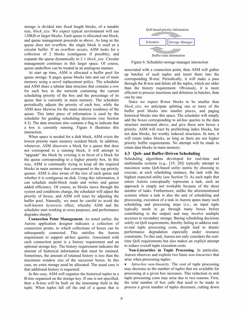
Queue Management. Each windowed operation requires a historical collection of tuples to be stored, equal to the size of the window. Moreover, if the network is currently saturated, then additional tuples may accumulate at various places in the network. As such, ASM must manage a collection of variable length queues of tuples. There is one queue at the output of each box, which is shared by all successor boxes. Each such successor box maintains two pointers into this queue. The head indicates the oldest tuple that this box has not processed. The tail, in contrast, indicates the oldest tuple that the box needs. The head and tail indicate box’s current window, which slides as new tuples are processed. ASM will keep track of these collections of pointers, and can normally discard tuples in a queue that are older than the oldest tail pointing into the queue. In summary, when a box produces a new tuple, it is added to the front of the queue. Eventually, all successor boxes process this tuple and it falls out of all of their windows and can be discarded. Figure 5 illustrates this model by depicting a two-way branch scenario where two boxes, b1 and b2, share the same queue (“w”s refer to window sizes).

Normally, queues of this sort are stored as main memory data structures. However, ASM must be able to scale arbitrarily, and has chosen a different approach. Disk

time

b1

w1= 5

tail head

w2= 9

b2tail head

youngesttuple

oldesttuple

can bediscarded

Figure 5: Queue organization

5

storage is divided into fixed length blocks, of a tunable size, block_size. We expect typical environment will use 128KB or larger blocks. Each queue is allocated one block, and queue management proceeds as above. As long as the queue does not overflow, the single block is used as a circular buffer. If an overflow occurs, ASM looks for a collection of 2 blocks (contiguous if possible), and expands the queue dynamically to 2 × block_size. Circular management continues in this larger space. Of course, queue underflow can be treated in an analogous manner.

Storage Manager

QoS-based priority information

Buffer-state information

Scheduler

Figure 6: Scheduler-storage manager interaction

At start up time, ASM is allocated a buffer pool for queue storage. It pages queue blocks into and out of main memory using a novel replacement policy. The scheduler and ASM share a tabular data structure that contains a row for each box in the network containing the current scheduling priority of the box and the percentage of its queue that is currently in main memory. The scheduler periodically adjusts the priority of each box, while the ASM does likewise for the main memory residency of the queue. This latter piece of information is used by the scheduler for guiding scheduling decisions (see Section 4.3). The data structure also contains a flag to indicate that a box is currently running. Figure 6 illustrates this interaction.

When space is needed for a disk block, ASM evicts the lowest priority main memory resident block. In addition, whenever, ASM discovers a block for a queue that does not correspond to a running block, it will attempt to “upgrade” the block by evicting it in favor of a block for the queue corresponding to a higher priority box. In this way, ASM is continually trying to keep all the required blocks in main memory that correspond to the top priority queues. ASM is also aware of the size of each queue and whether it is contiguous on disk. Using this information, it can schedule multi-block reads and writes and garner added efficiency. Of course, as blocks move through the system and conditions change, the scheduler will adjust the priority of boxes, and ASM will react by adjusting the buffer pool. Naturally, we must be careful to avoid the well-known hysteresis effect, whereby ASM and the scheduler start working at cross purposes, and performance degrades sharply.

Connection Point Management. As noted earlier, the Aurora application designer indicates a collection of connection points, to which collections of boxes can be subsequently connected. This satisfies the Aurora requirement to support ad-hoc queries. Associated with each connection point is a history requirement and an optional storage key. The history requirement indicates the amount of historical information that must be retained. Sometimes, the amount of retained history is less than the maximum window size of the successor boxes. In this case, no extra storage need be allocated. The usual case is that additional history is requested.

In this case, ASM will organize the historical tuples in a B-tree organized on the storage key. If one is not specified, then a B-tree will be built on the timestamp field in the tuple. When tuples fall off the end of a queue that is

associated with a connection point, then ASM will gather up batches of such tuples and insert them into the corresponding B-tree. Periodically, it will make a pass through the B-tree and delete all the tuples, which are older than the history requirement. Obviously, it is more efficient to process insertions and deletions in batches, than one by one.

Since we expect B-tree blocks to be smaller than block_size, we anticipate splitting one or more of the buffer pool blocks into smaller pieces, and paging historical blocks into this space. The scheduler will simply add the boxes corresponding to ad-hoc queries to the data structure mentioned above, and give these new boxes a priority. ASM will react by prefetching index blocks, but not data blocks, for worthy indexed structures. In turn, it will retain index blocks, as long as there are not higher priority buffer requirements. No attempt will be made to retain data blocks in main memory. 4.3 QoS- and Buffer-Driven Scheduling Scheduling algorithms developed for real-time and multimedia systems (e.g., [19, 20]) typically attempt to maximize some QoS-based utility metric by choosing to execute, at each scheduling instance, the task with the highest expected utility (see Section 5). As each tuple that enters Aurora conceptually represents a task, such an approach is simply not workable because of the sheer number of tasks. Furthermore, unlike the aforementioned systems where a task is also the unit of scheduling and processing, execution of a task in Aurora spans many such scheduling and processing steps (i.e., an input tuple typically needs to go through many boxes before contributing to the output) and may involve multiple accesses to secondary storage. Basing scheduling decisions solely on QoS requirements, thereby failing to address end-to-end tuple processing costs, might lead to drastic performance degradation especially under resource constraints. To this end, Aurora not only considers the real-time QoS requirements but also makes an explicit attempt to reduce overall tuple execution costs.

Non-Linearities in Tuple Processing. In particular, Aurora observes and exploits two basic non-linearities that arise when processing tuples: • Intra-box non-linearity. The cost of tuple processing may decrease as the number of tuples that are available for processing at a given box increases. This reduction in unit tuple processing costs may arise due to two reasons. First, the total number of box calls that need to be made to process a given number of tuples decreases, cutting down

6

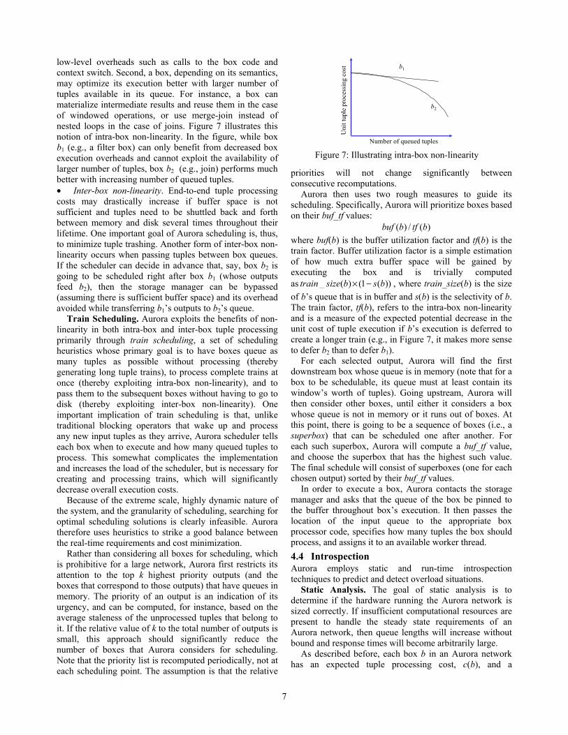
low-level overheads such as calls to the box code and context switch. Second, a box, depending on its semantics, may optimize its execution better with larger number of tuples available in its queue. For instance, a box can materialize intermediate results and reuse them in the case of windowed operations, or use merge-join instead of nested loops in the case of joins. Figure 7 illustrates this notion of intra-box non-linearity. In the figure, while box b1 (e.g., a filter box) can only benefit from decreased box execution overheads and cannot exploit the availability of larger number of tuples, box b2 (e.g., join) performs much better with increasing number of queued tuples.

Number of queued tuples

Uni

t tup

le p

roce

ssin

g co

st b1

b2

Figure 7: Illustrating intra-box non-linearity

• Inter-box non-linearity. End-to-end tuple processing costs may drastically increase if buffer space is not sufficient and tuples need to be shuttled back and forth between memory and disk several times throughout their lifetime. One important goal of Aurora scheduling is, thus, to minimize tuple trashing. Another form of inter-box non-linearity occurs when passing tuples between box queues. If the scheduler can decide in advance that, say, box b2 is going to be scheduled right after box b1 (whose outputs feed b2), then the storage manager can be bypassed (assuming there is sufficient buffer space) and its overhead avoided while transferring b1’s outputs to b2’s queue.

Train Scheduling. Aurora exploits the benefits of non-linearity in both intra-box and inter-box tuple processing primarily through train scheduling, a set of scheduling heuristics whose primary goal is to have boxes queue as many tuples as possible without processing (thereby generating long tuple trains), to process complete trains at once (thereby exploiting intra-box non-linearity), and to pass them to the subsequent boxes without having to go to disk (thereby exploiting inter-box non-linearity). One important implication of train scheduling is that, unlike traditional blocking operators that wake up and process any new input tuples as they arrive, Aurora scheduler tells each box when to execute and how many queued tuples to process. This somewhat complicates the implementation and increases the load of the scheduler, but is necessary for creating and processing trains, which will significantly decrease overall execution costs.

Because of the extreme scale, highly dynamic nature of the system, and the granularity of scheduling, searching for optimal scheduling solutions is clearly infeasible. Aurora therefore uses heuristics to strike a good balance between the real-time requirements and cost minimization.

Rather than considering all boxes for scheduling, which is prohibitive for a large network, Aurora first restricts its attention to the top k highest priority outputs (and the boxes that correspond to those outputs) that have queues in memory. The priority of an output is an indication of its urgency, and can be computed, for instance, based on the average staleness of the unprocessed tuples that belong to it. If the relative value of k to the total number of outputs is small, this approach should significantly reduce the number of boxes that Aurora considers for scheduling. Note that the priority list is recomputed periodically, not at each scheduling point. The assumption is that the relative

priorities will not change significantly between consecutive recomputations.

Aurora then uses two rough measures to guide its scheduling. Specifically, Aurora will prioritize boxes based on their buf_tf values:

( ) / ( )buf b tf b where buf(b) is the buffer utilization factor and tf(b) is the train factor. Buffer utilization factor is a simple estimation of how much extra buffer space will be gained by executing the box and is trivially computed as _ ( ) (1 ( ))ain size b s b× −tr , where train_size(b) is the size of b’s queue that is in buffer and s(b) is the selectivity of b. The train factor, tf(b), refers to the intra-box non-linearity and is a measure of the expected potential decrease in the unit cost of tuple execution if b’s execution is deferred to create a longer train (e.g., in Figure 7, it makes more sense to defer b2 than to defer b1).

For each selected output, Aurora will find the first downstream box whose queue is in memory (note that for a box to be schedulable, its queue must at least contain its window’s worth of tuples). Going upstream, Aurora will then consider other boxes, until either it considers a box whose queue is not in memory or it runs out of boxes. At this point, there is going to be a sequence of boxes (i.e., a superbox) that can be scheduled one after another. For each such superbox, Aurora will compute a buf_tf value, and choose the superbox that has the highest such value. The final schedule will consist of superboxes (one for each chosen output) sorted by their buf_tf values.

In order to execute a box, Aurora contacts the storage manager and asks that the queue of the box be pinned to the buffer throughout box’s execution. It then passes the location of the input queue to the appropriate box processor code, specifies how many tuples the box should process, and assigns it to an available worker thread. 4.4 Introspection Aurora employs static and run-time introspection techniques to predict and detect overload situations.

Static Analysis. The goal of static analysis is to determine if the hardware running the Aurora network is sized correctly. If insufficient computational resources are present to handle the steady state requirements of an Aurora network, then queue lengths will increase without bound and response times will become arbitrarily large.

As described before, each box b in an Aurora network has an expected tuple processing cost, c(b), and a

7

4.5 Load Shedding selectivity, s(b). If we also know the expected rate of tuple production r(d) from each data source d, then we can use the following static analysis to ascertain if Aurora is sized correctly.

When an overload is detected as a result of static or dynamic analysis, Aurora attempts to reduce the volume of Aurora tuple processing via load shedding. The naïve approach to load shedding involves dropping tuples at random points in the network in an entirely uncontrolled manner. This is similar to dropping overflow packets in packet-switching networks [28], and has two potential problems: (1) overall system utility might be degraded more than necessary; and (2) application semantics might be arbitrarily affected. In order to alleviate these problems, Aurora relies on QoS information to guide the load shedding process. We now describe two load shedding schemes that differ in the way they exploit QoS information.

From each data source, we begin by examining the immediate downstream boxes: if box bi is directly downstream from data source di, then, for the system to be stable, the throughput of bi should be at least as large as the input data rate; i.e.,

1/ ( ) ( )i ic b r d≥ We can then calculate the output data rate from bi as:

(1/ ( ), ( )) ( )i imin c b r d s b× i Proceeding iteratively, we can compute the output data

rate and computational requirements for each box in an Aurora network. We can then calculate the minimum aggregate computational resources required per unit time, min_cap, for stable steady-state operation. Clearly, the Aurora system with a capacity C cannot handle the expected steady state load if C is smaller than min_cap. Furthermore, the response times will assuredly suffer under the expected load of ad-hoc queries if

Load Shedding by Dropping Tuples. The first approach addresses the former problem mentioned above: it attempts to minimize the degradation (or maximize the improvement) in the overall system QoS; i.e., the QoS values aggregated over all the outputs. This is accomplished by dropping tuples on network branches that terminate in more tolerant outputs. _C H min cap× <

If load shedding is triggered as a result of static analysis, then we cannot expect to use delay-based or value-based QoS information (without assuming the availability of a priori knowledge of the tuple delays or frequency distribution of values). On the other hand, if load shedding is triggered as a result of dynamic analysis, we can also use delay-based QoS graphs if available.

Clearly, this is an undesirable situation and can be corrected by redesigning applications to change their resource requirements, by supplying more resources to increase system capacity, or by load shedding.

Dynamic Analysis. Even if the system has sufficient resources to execute a given Aurora network under expected conditions, unpredictable, long-duration spikes in input rates may deteriorate performance to a level that renders the system useless. We now describe two run-time techniques to detect such cases.

We use a greedy algorithm to perform load shedding. Let us initially describe the static load shedding algorithm driven by drop-based QoS graphs. We first identify the output with the smallest negative slope for the corresponding QoS graph. We move horizontally along this curve until there is another output whose QoS curve has a smaller negative slope at that point. This horizontal difference gives us an indication of the output tuples to drop (i.e., the selectivity of the drop box to be inserted) that would result in the minimum decrease in the overall QoS. We then move the corresponding drop box as far upstream as possible until we find a box that affects other outputs (i.e., a split point), and place the drop box at this point. Meanwhile, we can calculate the amount of recovered resources. If the system resources are still not sufficient, then we repeat the process.

Our first technique for detecting an overload relies on the use of delay-based QoS information, if available. Aurora timestamps all tuples from data sources as they arrive. Furthermore, all Aurora operators preserve the tuple timestamps as they produce output tuples (if an operator has multiple input tuples, then the earlier timestamp is preserved). When Aurora delivers an output tuple to an application, it checks the corresponding delay-based QoS graph (Figure 4b) for that output to ascertain that the delay is at an acceptable level (i.e., the output is in the good zone).

If delay-based QoS information is not available to guide Aurora in detecting abnormal operation, then Aurora employs a somewhat cruder technique. Specifically, Aurora watches its internal dispatching queue for evidence of sustained growth of one or more of the logical queues (in front of some box(es)). If a buildup is observed for a period of time exceeding a threshold, then Aurora takes corrective action. Of course, longer queue lengths do not necessarily mean that the delivered QoS is bad or unacceptable (e.g., consider train scheduling). Unless delay-based QoS information is available, however, this is the most reliable piece of information used to trigger load shedding.

For the run-time case, the algorithm is similar except that we can use delay-based QoS graphs to identify the problematic outputs, i.e., the ones which are beyond their delay thresholds, and we repeat the load shedding process until the latency goals are met.

In general, there are two subtleties in dynamic load shedding. First, drop boxes inserted by the load shedder should be among the ones that are given higher priority by the scheduler. Otherwise, load shedding will be ineffective in reducing the load of the system. Therefore, the load shedder simply does not consider the inactive (i.e., low priority) outputs, which are indicated by the scheduler.

8

Secondly, the algorithm tries to move the drop boxes as close to the sources as possible to discard tuples before they redundantly consume any resources. On the other hand, if there is a box with a large existing queue, it makes sense to temporarily insert the drop box at that point rather than trying to move it upstream closer towards the data sources.

Presumably, the application is coded so that it can tolerate missing tuples from a data source caused by communication failures or other problems. Hence, load shedding simply artificially introduces additional missing tuples. Although the semantics of the application are somewhat different, the harm should not be too damaging.

Semantic Load Shedding by Filtering Tuples. The load shedding scheme described above effectively reduces the amount of Aurora processing by dropping randomly selected tuples at strategic points in the network. While this approach attempts to minimize the loss in overall system utility, it fails to control the impact of the dropped tuples on application semantics. Semantic load shedding addresses this limitation by using value-based QoS information, if available (recall that value-based QoS graphs specify the relative importance of various values for a given output). Specifically, semantic load shedding drops tuples in a more controlled way; i.e., it drops less important tuples, rather than random ones, using filters.

If value-based QoS information is available, then Aurora can watch each output and build up a histogram containing the frequency with which value ranges have been observed. In addition, Aurora can calculate the expected utility of a range of outputs by multiplying the QoS values with the corresponding frequency values for every interval and then summing these values. To shed load, Aurora identifies the output with the lowest utility interval; converts this interval to a filter predicate; and then, as before, attempts to propagate the corresponding filter box as far upstream as possible to a split point. This strategy, which we refer to as backward interval propagation, admittedly has limited scope because it requires the application of the inverse function for each operator passed upstream (Aurora boxes do not necessarily have inverses). An alternative strategy, forward interval propagation, estimates a proper filter predicate and propagates it in downstream direction to see what results at the output. By trial-and-error, Aurora can converge on a desired filter predicate. Note that a combination of these two strategies can also be utilized. First, Aurora can apply backward propagation until a box, say b, whose operator’s inverse is difficult to compute. Aurora can then apply forward propagation between the insertion location of the filter box and b. This algorithm can be applied iteratively until sufficient load is shed.

5 Related Work A special case of Aurora processing is as a continuous query system. A continuous query system like Niagara [6] is concerned with combining multiple data sources in a

wide area setting, while we are initially focusing on the construction of a general stream processor that can process very large numbers of streams.

Indexing queries [2] is an important technique for enhancing the performance of large-scale filtering applications (e.g., publish/subscribe). In Aurora, this would correspond to a merge of some inputs followed by a fanout to a large number of filter boxes. Query indexing would be useful here, but it represents only one Aurora processing idiom.

As in Aurora, active databases [21, 22] are concerned with monitoring conditions. These conditions can be a result of any arbitrary update on the stored database state. In our setting, updates are append-only, thus requiring different processing strategies for detecting monitored conditions. Triggers evaluate conditions that are either true or false. Our framework is general enough to support queries over streams or the conversion of these queries into monitored conditions. There has also been extensive work on making active databases highly scalable (e.g., [10]). Similar to continuous query research, these efforts have focused on query indexing, while Aurora is constructing a more general system.

Adaptive query processing techniques (e.g., [3, 14, 27]) address efficient query execution in unpredictable and dynamic environments by revising the query execution plan as the characteristics of incoming data changes. Of particular relevance is the Eddies work [3]. Unlike traditional query processing where every tuple from a given data source gets processed in the same way, each tuple processed by an Eddy is dynamically routed to operator threads for partial processing, with the responsibility falling upon the tuple to carry with it its processing state. Recent work [18] extended Eddies to support the processing of queries over streams, mainly by permitting Eddies systems to process multiple queries simultaneously and for unbounded lengths of time. The Aurora architecture bears some similarity to that of Eddies in its division of a single query’s processing into multiple threads of control (one per query operator). However, queries processed by Eddies are expected to be processed in their entirety; there is neither the notion of load shedding, nor quality of service.

Directly related work on stream data query processing architectures shares many of the goals and target application domains with Aurora. The Streams project [4] attempts to provide complete DBMS functionality along with support for continuous queries over streaming data. Aurora’s main emphasis is on efficiently supporting sophisticated continuous queries over a large number of potentially very fast data streams, thus sacrificing some traditional database functionality such as transactions. The Fjords architecture [17] combines querying of push-based sensor sources with pull-based traditional sources by embedding the pull/push semantics into queues between query operators. It is fundamentally different from Aurora in that operator scheduling is governed by a combination of schedulers specific to query threads and operator-queue

9

interactions. Tribeca [26] is an extensible, stream-oriented data processor designed specifically for supporting network traffic analysis. While Tribeca incorporates many of the stream operators and compile-time optimizations Aurora supports, it does not address crucial run-time issues such as scheduling or load shedding. Furthermore, Tribeca does not have the concept of ad-hoc queries, and, thus, does not address relevant storage organization issues.

Tools for mining of stream-based data have received considerable attention lately. Some tools only allow one pass over stored stream data (e.g., [12]), whereas others (e.g., [13]) are interested in addressing data mining problems and, thus, require multiple passes.

Work in sequence databases [25] defined sequence definition and manipulation languages over discrete data sequences. The Chronicle data model [15] defined a restricted view definition and manipulation language over append-only sequences. Aurora’s algebra extends relevant aspects of previous proposals by proposing a binary windowed operator (i.e., join), which is indispensable for continuous query execution over data streams.

Our work is also relevant to materialized views [9], which are essentially stored continuous queries that are re-executed (or incrementally updated) as their base data are modified. However, Aurora’s notion of continuous queries differs from materialized views primarily in that Aurora updates are append-only, thus, making it much easier to incrementally materialize the view. Also, query results are streamed (rather than stored); and high stream data rates may require load shedding or other approximate query processing techniques that trade off efficiency for result accuracy.

Our work is likely to benefit from and contribute to the considerable research on temporal databases [20] and main-memory databases [7], which assume an HADP model, whereas Aurora proposes a DAHP model that builds streams as fundamental Aurora objects. We can also benefit from the literature on real-time databases [16, 20]. In a real-time database system, transactions are assigned timing constraints and the system attempts to ensure a degree of confidence in meeting these timing requirements. The Aurora notion of QoS specification extends the soft and hard deadlines employed in real-time databases to general utility functions. Furthermore, real-time databases associate deadlines with individual transactions, whereas Aurora associates QoS curves with outputs from stream processing and, thus, has to support continuous timing requirements.

There has been extensive research on scheduling tasks in real-time and multimedia systems and databases [19, 20]. The proposed approaches are commonly deadline- (or QoS-) driven; i.e., at each scheduling point, the task that has the earliest deadline or one that is expected to provide the highest QoS (e.g., throughput) is identified and scheduled. In Aurora, such an approach is not only impractical because of the sheer number of potentially schedulable tasks (i.e., tuples), but is also inefficient because of the implicit assumption that all tasks are

memory-resident and are scheduled and executed in their entirety. Note that Eddies scheduling [3, 18] addresses the latter issue by favoring memory-resident tuples for execution. To the best of our knowledge, however, our train scheduling approach is unique in its ability to reduce overall execution costs by exploiting intra- and inter-box non-linearities described here.

The work of [27] takes a scheduling-based approach to query processing; however, they do not address continuous queries, are primarily concerned with data rates that are too slow (we also consider rates that are too high), and they only address query plans that are trees with single outputs.

The congestion control problem in data networks [28] is relevant to Aurora and its load shedding mechanism. Load shedding in networks typically involves dropping individual packets randomly, based on timestamps, or using (application-specified) priority bits. Despite conceptual similarities, there are also some fundamental differences between network load shedding and Aurora load shedding. First, unlike network load shedding which is inherently distributed, Aurora is aware of the entire system state and can potentially make more intelligent shedding decisions. Second, Aurora uses QoS information provided by the external applications to trigger and guide load shedding. Third, Aurora’s semantic load shedding approach not only attempts to minimize the degradation in overall system utility, but also quantifies the imprecision due to dropped tuples.

Aurora load shedding is also related to approximate query answering (e.g., [11]) and data reduction and summary techniques [5, 8], where result accuracy is traded for efficiency. By throwing away data, Aurora bases its computations on sampled data, effectively producing approximate answers using data sampling. The unique aspect of our approach is that our sampling is driven by QoS specifications.

6 Conclusions Monitoring applications are those where streams of information, triggers, real-time requirements, and imprecise data are prevalent. Traditional DBMSs are based on the HADP model, and thus cannot provide adequate support for such applications. In this paper, we have described the architecture of Aurora, a DAHP system, oriented towards monitoring applications. We argued that providing efficient support for these demanding applications not only require critically revisiting many existing aspects of database design and implementation, but also require developing novel proactive data storage and processing concepts and techniques.

In this paper, we first presented the basic Aurora architecture, along with the primitive building blocks for workflow processing. We followed with several heuristics for optimizing a large Aurora network. We then focused on run-time data storage and processing issues, discussing in detail storage organization, real-time scheduling,

10

introspection, and load shedding, and proposed novel solutions in all these areas.

We have started to implement the proposed architecture and shortly expect to have an initial prototype, which we will use to verify the effectiveness and practicality of the Aurora model and related algorithms. In terms of future work, we identified two important research directions. First, we are extending our data and processing model to cope with missing and imprecise data values, which are common in applications involving sensor-generated data streams. Second, we are working on a distributed Aurora architecture that will enable operators to be pushed closer to the data sources, potentially yielding significantly improved scalability, energy use, and bandwidth efficiency.

References [1] Informix White Paper. Time Series: The Next Step for

Telecommunications Data Management. [2] M. Altinel and M. J. Franklin. Efficient Filtering of

XML Documents for Selective Dissemination of Information. In Proc. of the 26th VLDB Conf., 2000.

[3] R. Avnur and J. Hellerstein. Eddies: Continuously Adaptive Query Processing. In Proc. of the SIGMOD Conf., Dallas, TX, 2000.

[4] S. Babu and J. Widom. Continuous Queries over Data Streams. SIGMOD Record, 30(3):109-120, 2001.

[5] D. Barbara, W. DuMouchel, C. Faloutsos, P. J. Haas, J. M. Hellerstein, Y. E. Ioannidis, H. V. Jagadish, T. Johnson, R. T. Ng, V. Poosala, K. A. Ross, and K. C. Sevcik. The New Jersey Data Reduction Report. IEEE Data Engineering Bulletin, 20(4):3-45, 1997.

[6] J. Chen, D. J. DeWitt, F. Tian, and Y. Wang. NiagaraCQ: A Scalable Continuous Query System for Internet Databases. In Proc. of the SIGMOD Conf., Dallas, TX, 2000.

[7] H. Garcia-Molina and K. Salem. Main Memory Database Systems: An Overview. IEEE Transactions on Knowledge and Data Engineering (TKDE), 4(6):509-516, 1992.

[8] J. Gehrke, F. Korn, and D. Srivastava. On Computing Correlated Aggregates over Continual Data Streams. In Proc. of the SIGMOD Conf., Santa Barbara, CA, 2001.

[9] A. Gupta and I. S. Mumick. Maintenance of Materialized Views: Problems, Techniques, and Applications. IEEE Data Engineering Bulletin, 18(2):3-18, 1995.

[10] E. N. Hanson, C. Carnes, L. Huang, M. Konyala, L. Noronha, S. Parthasarathy, J. B. Park, and A. Vernon. Scalable Trigger Processing. In Proc. of the 15th ICDE, Sydney, Austrialia, 1999.

[11] J. M. Hellerstein, P. J. Haas, and H. J. Wang. Online Aggregation. In Proc. of the SIGMOD Conf., 1997.

[12] M. R. Henzinger, P. Raghavan, and S. Rajagopalan. Computing on Data Streams. Compaq Systems

Research Center, Palo Alto, California Technical Report TR-1998-011, May 1998.

[13] C. Hidber. Online Association Rule Mining. In Proceedings of the 1999 ACM SIGMOD International Conference on Management of Data, Philadelphia, PA, 1999.

[14] Z. G. Ives, D. Florescu, M. Friedman, A. Levy, and D. S. Weld. An Adaptive Query Execution System for Data Integration. In Proc. of the SIGMOD Conf., Philadelphia, PA, 1999.

[15] H. V. Jagadish, I. S. Mumick, and A. Silberschatz. View Maintenance Issues for the Chronicle Data Model. In Proc. of the 14th PODS, 1995.

[16] B. Kao and H. Garcia-Molina, “An Overview of Realtime Database Systems,” in Real Time Computing, W. A. Halang and A. D. Stoyenko, Eds.: Springer-Verlag, 1994.

[17] S. Madden and M. J. Franklin. Fjording the Stream: An Architecture for Queries over Streaming Sensor Data. In Proc. of the 18th ICDE, 2002.

[18] S. R. Madden, M. A. Shaw, J. M. Hellerstein, and V. Raman. Continuously Adaptive Continuous Queries Over Streams. In Proc. of the SIGMOD Conf., Wisconsin, USA, 2002.

[19] J. Nieh and M. S. Lam. The Design, Implementation and Evaluation of SMART: A Scheduler for Multimedia Applications. In Proc. 16th ACM Symposium on OS Principles, 1997.

[20] G. Ozsoyoglu and R. T. Snodgrass. Temporal and Real-Time Databases: A Survey. IEEE Transactions on Knowledge and Data Engineering (TKDE), 7(4):513-532, 1995.

[21] N. Paton and O. Diaz. Active Database Systems. ACM Computing Surveys, 31(1):63-103, 1999.

[22] U. Schreier, H. Pirahesh, R. Agrawal, and C. Mohan. Alert: An Architecture for Transforming a Passive DBMS into an Active DBMS. In Proc. of the 17th VLDB Conf., Barcelona, Spain, 1991.

[23] T. K. Sellis. Multiple-Query Optimization. ACM Transactions on Database Systems (TODS), 13(1):23-52, 1988.

[24] T. K. Sellis and S. Ghosh. On the Multiple-Query Optimization Problem. IEEE Transactions on Knowledge and Data Engineering (TKDE), 2(2):262-266, 1990.

[25] P. Seshadri, M. Livny, and R. Ramakrishnan. The Design and Implementation of a Sequence Database System. In Proc. of the 22th VLDB, India, 1996.

[26] M. Sullivan and A. Heybey. Tribeca: A System for Managing Large Databases of Network Traffic. In Proc. of the USENIX Annual Technical Conf., New Orleans, LA, 1998.

[27] T. Urhan and M. J. Franklin. Dynamic Pipeline Scheduling for Improving Interactive Query Performance. In Proc. of the VLDB Conf., 2001.

[28] C. Yang and A. V. S. Reddy. A Taxonomy for Congestion Control Algorithms in Packet Switching Networks. IEEE Network, 9(5):34-44, 1995.

11

Appendix 1. Aurora Query Operator Semantics 4. Merge (+): Merge performs the union of tuples from separate but compatible streams (i.e., those that have the same index types, units of measure, and tuple schemas). �

A stream is a potentially infinite set of tuples ordered by index values (such as timestamps or integer positions). More formally, a stream, S, is a set of (index value, tuple) pairs (stream elements):

1 2 1S S S S+ = ∪ 2 �S = {(i1, t1), (i2, t2), … , (in, tn), …} 5. Resample (ρ): Resample predicts elements in one

stream for every index value represented in another. The prediction is made based on a prediction function, f, and a window size, w, that indicates how much history from S1 must be used for prediction. Thus, for any streams, S1 and S2 with compatible index types; window size, w; and function, f:

such that index values, ij, belong to an index type (below), and all tuples, tj, belong to the same schema.

An index type is a totally ordered type that is associated with a unit measure, which defines minimal increments in index values. For example, if the index type consists of timestamps (as in stock data), then the associated unit measure might be 15 min or 1 hour depending on the maximum frequency of stock data. Unit measures permit expression of distances between elements, and window sizes within queries. Index types include the following operations:

, 1 2 2

1

( , ) {( , ( ')) | [ ] ,

' {( ', ) | ( , ') }}w f S S i f S S i

S i x S i i w

ρ = ≠

= ∈ ∆ ≤

∅

,

≤

≠

S

�

6. Join (>< ) Join correlates pairs of streams with compatible indexes (i.e., the same types and unit measures). Elements from different streams are joined provided that the distance between them (as determined by their indexes) is within a given window size. Thus, for any streams S1 and S2; predicate, p; function, f; and window size, w:

• Ordering relations (<, >, ≤,� ≥): Because the index type is a total order, it must be the case for any elements of the index type, i1 and i2, that either i1 < i2, i2 < i1, or i1 = i2.

• Position Arithmetic (+, -, %): For any index value, i, i + k is the index value that is k unit measures more than i. For example, if i is a timestamp-based index type with unit measure, 1 hour, then 15:00 + 3 = 18:00. ‘-’ is defined similarly. ‘%’ performs modular arithmetic on index values.

, ,

1 1 2 2

1 2

1 2 { ( , ) |

( [ ] , [ ] , ( , ), [ ], [ ]), ( , )}

p f wS S f x y i

j S i S S j S i jw x S i y S j p x y

= ∃

⊆ ⊆ ∆∈ ∈

><

• Distance (∆): ∆ (i1, i2) is the integer distance (in unit measures) between index values i1 and i2.

7. Drop (δ): Drop is a special kind of filter that filters streams according to index values. Specifically, given a period of k units, δk would block all elements for every kth index value. More formally, given a positive integer, k:

In defining the formal semantics of Aurora’s query operators, we adopt the following shorthand notation applicable to any stream,

S = {(i1, t1), (i2, t2),…, (in, in), …}: ( ) {( , ) | ( , ) , % 0}k S i t i t S i kδ = ∈ 1. S [ik] = {(ik, tk) | (ik, tk) ∈ S} 2. S [im…in] = {(ik, tk) | (ik, tk) ∈ S, im ≤ ik ≤ in } 3. index (ik, tk) = ik, value (ik, tk) = tk Appendix 2. Operator Commutativity Properties

Aurora’s query operations all accept one or more input streams and produce a single output stream:

This appendix treats conditional commutativity in more detail. In Table 2, we present the commutativity information presented in Table 1 with all the conditional cases numbered. What follows are the precise conditions for commutativity for each of the ten cases.

1. Filter (σ): σp(S) returns stream elements in S that satisfy the predicate, p:

( ) { | , ( )}p S x x S p xσ = ∈ 1. , if attributes referred to

in are unchanged by . ( ( )) ( ( ))p f f pSσ µ µ σ≡

p f2. Map (µ): µf(S) applies the function f to every

stream element in S: ( ) { ( ) | }f S f x x Sµ = ∈ 2. , if 1 2 1 2( ( , , )) ( , ( ), )p pf S S f S Sσ ρ ρ σ≡

3. Windowed-Map (Μ): Given function f, that maps a subset of consecutive stream elements (window) to another steam element, Μf,w(S) returns the stream resulting from applying f to every set of elements in S whose index values differ by at most w unit measures:

i. is always (i.e., ) on both andp true ( ) 1selectivity p =

1 2, )S1S ( ,f Sρ , or ii. 2 1( ) ( ( ))index index pS Sµ µ σ⊆ .

3. , where

, , 1 2 , , 1 2( ( , )) ( , )p q concat w p q concat wS S S Sσ ∧≡>< ><

, ( ) { ( ') | ( ' [ .. 1])}f wM S f S d S S d d w= ∃ = + −

12

filter map w. map merge resample join drop

filter yes map 1 4

w. map no 5 8 merge yes yes no yes

resample 2 6 no no 9 join 3 7 no no no 10 drop yes yes no yes no no yes

Table 2: Detailed operator commutativity table

13

S

S

)S

1 2, ,

, , 1 2

1

2

, , 1 2

1

2

, ,

( , )

( ( ), ),

if is defined on and is not defined on

( , ( )),

if is not defined on and is defined on

(

p q concat w

q concat w p

q concat w p

q concat w

S S

S S

p Sp S

S S

p Sp S

σ

σ

σ

∧≡><

><

><

><

1 2

1 2

1 2

, , 1 2

1 2

1 2

1 1

2

( ), ( )),

if is defined on both and ( ( ), ( )),

if is not defined on either or , but , where is defined on and is defi

p p

q concat w p p

S S

p SS S

p Sp p p

p Sp

σ

σ σ

= ∧

><

2

, , 1 2

ned on ( , ), otherwise.q concat w

SS S

><

In the above formulation, concat, which stands for concatenation of two tuples, is given as the default combining function of the join operator. In fact, any function that keeps the attributes of the joined tuples that are also referred by predicate could be used instead.

p

4. , if . ( ( )) ( ( ))f g g fS Sµ µ µ µ≡ f g g fο ο=5. , ,( ( )) ( ( )f g w g w fSµ µ µ µ≡

( ( [ .. 1])) ( ( [ ]), ( [ 1]),...,f g S i i w

g f S i f S i f+ − =

, if for any index i ,

. ( [ 1]))S i w+ + −

In other words, should distribute overf g . Note that this formulation assumes that indices act as keys.

6. , if 1 2 1 2( ( , , )) ( , ( ), )g gf S S f S Sµ ρ ρ µ≡i. introduces no new values in (e.g.,

is a step-wise constant function), or ff

1S

ii. g is the identity function, or iii. 2 1( ) (index indexS S )µ µ⊆ .

7. , where , , 1 2

, , 1 2

( ( ,

( , )f p concat w

p concat f w

S S

S Sο

µ ≡><

><

))

S

S

, , 1 2

, , 1 2

1

2

, , 1 2

1

2

, , 1

( , )

( ( ), ),

if is defined on and is not defined on

( , ( )),

if is not defined on and is defined on

( ( ),

p concat f w

p concat w f

p concat w f

p concat w f

S S

S S

f Sf S

S S

f Sf S

S

ο

µ

µ

µ

≡><

><

><

><

1 2

2

1 2

, , 1 2

1 2

1 2

1 1

2 2

,

( )),

if is defined on both and ( ( ), ( )),

if is not defined on either or , but , where is defined on

and is defined on

f

p concat w f f

p

S

f SS S

f Sf f ff S

f S

µ

µ µ

ο=

><

>< , 1 2( , ), otherwiseconcat w S S

and attributes referred to in are unchanged by .

pf

8. , if for any

, , , ,( ( )) ( ( ))f w g w g w f wS Sµ µ µ µ≡( ( [ .. 1]), ( [ 1..

( [ 1.. 2]))( ( [ .. 1]), ( [ 1..

( [ 1.. 2]))

f g S i i u g S i ig S i w i u w

g f S i i u f S i if S i w i u w

+ − ++ − + + −

+ − ++ − + + −

i]),..,

]),..,

u

u

+=

+

9. 1 3 2 1 3 2( , ( , , ), ) ( , ( , , ), )f g S S S g f S S Sρ ρ ρ ρ≡f g=

, if .

10. , , , , , 1 2 3

, , 1 , , 2 3

( ( , ),

( , ( , ))p concat w q concat u

q concat u p concat w

S S S

S S

≡>< ><

>< ><

)

S

if is defined on attributes of and S , and is defined on attributes of and .

p 2S 3 q

1S 2S