®

The contents of this report reflect the views of the authors, who are responsible for the facts and the accuracy of the information presented herein. This document is disseminated under the sponsorship of the Department of Transportation

University Transportation Centers Program, in the interest of information exchange. The U.S. Government assumes no liability for the contents or use thereof.

Monitoring the Effects of Knickpoint Erosion on Bridge Pier and Abutment Structural Damage Due to Scour

Report # MATC-UI-UNL: 471/424 Final Report

A.N. Thanos Papanicolaou, Ph.D.ProfessorDepartment of Civil and Environmental EngineeringIIHR—Hydroscience & EngineeringUniversity of Iowa

David M. Admiraal, Ph.D.Associate ProfessorChristopher Wilson, Ph.D. Assistant Research ScientistClark KephartGraduate Research Assistant

2012A Cooperative Research Project sponsored by the U.S. Department of Transportation Research and Innovative Technology Administration

25-1121-0001-471, 25-1121-0001-424

Monitoring the Effects of Knickpoint Erosion on Bridge Pier

and Abutment Structural Damage Due to Scour

A.N. Thanos Papanicolaou, Ph.D.

Professor

Department of Civil and Environmental Engineering

IIHR—Hydroscience & Engineering

University of Iowa

David M. Admiraal, Ph.D.

Associate Professor

Department of Civil Engineering

University of Nebraska–Lincoln

Christopher Wilson, Ph.D.

Assistant Research Scientist

IIHR—Hydroscience & Engineering

University of Iowa

Clark Kephart

Graduate Research Assistant

Department of Civil Engineering

University of Nebraska–Lincoln

A Report on Research Sponsored by

Mid-America Transportation Center

University of Nebraska-Lincoln

April 2012

ii

Technical Report Documentation Page 1. Report No.

25-1121-0001-471

(also reporting for 25-1121-0001-424)

2. Government Accession No.

3. Recipient's Catalog No.

4. Title and Subtitle

Monitoring the effects of knickpoint erosion on bridge pier and abutment

structural damage due to scour

5. Report Date

April 2012

6. Performing Organization Code

7. Author(s)

A. N. Thanos Papanicolaou, David Admiraal, Christopher Wilson, and Clark

Kephart

8. Performing Organization Report No.

25-1121-0001-471

(also reporting for 25-1121-0001-424)

9. Performing Organization Name and Address

Mid-America Transportation Center 2200 Vine St. PO Box 830851 Lincoln, NE 68583-0851

10. Work Unit No. (TRAIS)

11. Contract or Grant No.

12. Sponsoring Agency Name and Address

Research and Innovative Technology Administration

1200 New Jersey Ave., SE

Washington, D.C. 20590

13. Type of Report and Period Covered

Final Report

July 2010-April 2012

14. Sponsoring Agency Code

MATC TRB RiP No. 28504 15. Supplementary Notes

16. Abstract

The goal of this study was to conduct a field-oriented evaluation, coupled with advanced laboratory techniques, of channel

degradation in a stream of the Deep Loess Region of western Iowa, namely Mud Creek. The Midwestern United States is

an ideal place for such a study considering that ~$1 Billion of infrastructure and farmland has been lost recently to channel

degradation. A common form of channel degradation in this region is associated with the formation of knickpoints, which

naturally manifest as short waterfalls within the channel that migrate upstream. As flow plunges over a knickpoint face,

scouring of the downstream bed creates a plunge pool. This downcutting increases bank height, facilitating bank failure,

stream widening, and damage to critical bridge infrastructure. We conducted a state-of-the-art geotechnical analysis of the

sediments from the knickpoint face, plunge pool, and adjacent stream banks to determine the areas of the streambed near

the bridge infrastructure that favor knickpoint propagation. Soil characterization using particle size distributions and

Gamma Spectroscopy identified a stratigraphic discontinuity at the elevation where the knickpoint forms. An automated

surveillance camera was established to monitor the location of the knickpoint face relative to a fixed datum and provide a

first-order approximation of its migration rate, which was approximately 0.9 m over a 248-day study period. Surveys

conducted of the stream reach also facilitated information about knickpoint migration. Flow measurements using Large-

scale Particle Image Velocimetry were conducted during the study to understand the hydrodynamic conditions at the site.

The results of this research will assist local and federal transportation agencies in better understanding the following: (1)

principal geotechnical and hydrodynamic factors that control knickpoint propagation, (2) identify necessary data for

extraction and analysis to predict knickpoint formation, (3) provide mitigation measures such as grade control structures

(e.g., sheet-pile weirs, bank stabilization measures) near bridge crossings to control the propagation of knickpoints and

prevent further damage to downstream infrastructure.

17. Key Words

Knickpoint, Scour, Bridge Infrastructure Safety 18. Distribution Statement

19. Security Classif. (of this report)

Unclassified 20. Security Classif. (of this page)

Unclassified 21. No. of Pages

51

22. Price

iii

Table of Contents

Acknowledgements viii Disclaimer ix

Executive Summary x Chapter 1 Introduction 1

1.1 Problem Statement 1 1.2 Definitions 4 1.3 Previous Research 6

Chapter 3 Methodology 10 3.1 Study Site 10 3.2 Core Extraction 11

3.3 Core Parameterization 14 3.4 Knickpoint Propagation Using a Time-Lapse Camera 18 3.5 Knickpoint Propagation Using Survey Data 21

3.6 Flow Velocity Distributions Using LPIV 21 Chapter 4 Results 26

4.1 Geotechnical Analysis 26 4.2 Knickpoint Propagation 35 4.3 Flow Velocity Observations – LPIV 40

Chapter 5 Summary and Conclusions 43

References 49

iv

List of Figures

Figure 1.1 (a) Channel straightening of Mud Creek, IA in the 1950s. The

white line is the original channel. The blue line is the creek after straightening;

(b) Channel incision at Mud Creek. 1

Figure 1.2 Knickpoint formation. The circled area is a knickpoint in

Mud Creek, IA. 4 Figure 1.3 Knickpoint processes. A sketch of the steps involved in knickpoint

migration. 5

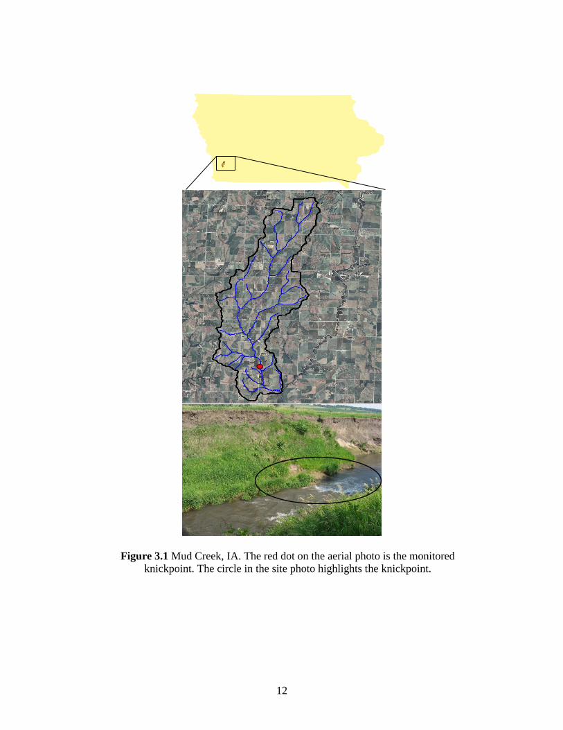
Figure 3.1 Mud Creek, IA. The red dot on the aerial photo is the monitored

knickpoint. The circle in the site photo highlights the knickpoint. 12

Figure 3.2 Core Collection. Cores from the stream banks near the knickpoint

face were collected using a Giddings probe and Shelby tube system. 13 Figure 3.3 Stratigraphic Interpretation. A close-up of the surface section for the

stream bank core used in the stratigraphy analysis. The ruler in

the image is in inches. 15 Figure 3.4 Gamma Scanner. The gamma scanner system at IIHR. Typical

results of a core’s density. 16 Figure 3.5 Measuring Core Bulk Density. A section of the stream bank core

was placed in a vertical frame. A 241

Am sealed source was moved up

and down the core length in conjunction with a gamma energy

detector on the other side of the core. The attenuation of the received

radioactivity was indication of the core density. 17

Figure 3.6 Time-lapse images collected on (a) September 15, 2011

(b) December 3, 2011, and (c) February 12, 2012. 20 Figure 3.7 Corrected Time-lapse images from (a) September 15, 2011

(b) December 3, 2011, and (c) February 12, 2012. 19 Figure 3.8 LPIV image samples: (a) original image sampled from LPIV video

and (b) rectified LPIV image. 23

Figure 3.9 Depiction of subareas associated with interrogation points used for

discharge calculations. 24

Figure 4.1 Stratigraphic Discontinuity. There appears to be a stratigraphic

discontinuity close to the knickpoint with a darker sediment

(in the black circle) overlaying a lighter-colored sediment

(in the red circle). 26

Figure 4.2 Particle Size Distribution. These graphs show key particle size

diameters of the sampled depth intervals in a stream bank core

from the study site. The d16, d50, and d84 for each interval are

plotted relative to depth. The red circle highlighting the 600-650 cm

depth interval corresponds to a coarsening of the overall particle size distribution,

as there are increases in the d50 and d84. This elevation corresponds to the top

elevation of the knickpoint face. 28

v

Figure 4.3 Soil Texture. The percentages of clay, silt, and sand for each depth interval

of a stream bank core from the study site. The red circle highlighting the

600-650 cm depth interval corresponds to a discontinuity in bank stratigraphy.

This discontinuity corresponds to the top elevation of the knickpoint face. 29

Figure 4.4 Soil Ternary Diagram. The soil texture of depth intervals in a stream

bank core based on USDA soil classifications and particle size measurements. Red

circles represent samples above 600 cm, and blue circles represent samples

below 600 cm. The 600-650 cm elevation corresponds to the top elevation

of the knickpoint face. There is a coarsening of sediment below this elevation, as

seen through a shift in the texture as the material becomes sandier. 31 Figure 4.5 Atterberg Limits. The Atterberg limits of select depth intervals were

measured using a fall cone. The samples were chosen because they had a

majority of fine particle sizes. Red circles represent samples above 600 cm,

and blue circles represent samples below 600 cm. The 600-650 cm elevation

corresponds to the top elevation of the knickpoint face. The samples are mostly

characterized as clay with low plasticity. 32 Figure 4.6 Surrogate Bulk Density. The density of a stream bank core was measured

using the attenuation of a gamma radiation source. These graphs show the depth

profile of attenuation count rates for a stream bank core. A high count rate

translates to high transmission of the gamma source through the core, so that

depth interval will have a lower bulk density. The red circles highlight shifts in the

depth profile. 33

Figure 4.7 Stream bed cores. The depth profile of the percent sand of cores

collected along a transect of the stream bed reach near the knickpoint. The zero level

represents the top of the knickpoint face. Old KP represents the core furthest

downstream where the knickpoint was in 2009. The transect moves upstream

as follows: Chute -> Sensors -> Current KP. There appears to be no

difference in the depth profiles; however, there is a coarsening four feet

below the surface. 35

Figure 4.8 Knickpoint migration between July 14, 2011 and March 16, 2012. 36 Figure 4.9 50 cm contours for surveyed data for (a) September 27, 2011, and

(b) March 21, 2012. 38 Figure 4.10 (a) Image of the knickpoint on March 18, 2011, prior to installation

of knickpoint monitoring equipment. Note the previous trench in the foreground

and the previous and new scour holes. (b) Plan view of the current knickpoint

location depicting the approximate location of the current trench. 39 Figure 4.11 Surface velocity distribution measured with LPIV on

(a) September 27, 2011, and (b) March 21, 2012. 41

vi

List of Tables

Table 4.1 Average percentages of sediment size fractions ........................................................... 29 Table 4.2 Summary of cross section discharge calculations, September 27, 2012 ...................... 42

Table 4.3 Summary of cross section discharge calculations, March 21, 2012 ............................. 43 Table 5.1 The main features of inspection form used by the Iowa DOT when inspecting

bridges that recently have experienced a major flood flow ............................................. 47

vii

List of Abbreviations

American Society of Testing and Materials (ASTM)

Hungry Canyons Alliance (HCA)

Iowa Department of Transportation (IDOT)

Large-scale Particle Image Velocimetry (LPIV)

Mid-America Transportation Center (MATC)

Minimum Quadratic Difference (MQD)

viii

Acknowledgments

This grant was awarded by the Mid-America Transportation Center (MATC). The

authors would like to thank Mr. Trevis Huff and Mr. John Thomas, who assisted with the field

work and provided the necessary guidance at the early stages of this project. The authors

additionally would like to thank the Natural Resources Conservation Service and Dr. Art Bettis

for assisting with the cores and their classification. Finally, the authors would like to thank, in

advance, the MATC staff for revising and processing this report.

About IIHR—Hydroscience & Engineering

IIHR—Hydroscience & Engineering is a unit of the College of Engineering at the

University of Iowa. It is one of the nation’s oldest and premier environmental fluids research and

engineering laboratories. IIHR seeks to educate students on conducting research in the broad

fields of river hydraulics, sediment transport, and watershed processes. IIHR has 44 faculty

members and research engineers at the Ph.D. level, 8 postdoctoral scholars, and about 113 M.S.

and Ph.D. graduate students. IIHR’s 30 staff members include administrative assistants

(including grant accounting and reporting support), IT support, and machine/electrical shop

engineers.

ix

Disclaimer

The contents of this report reflect the views of the authors, who are responsible for the

facts and the accuracy of the information presented herein. This document is disseminated under

the sponsorship of the U.S. Department of Transportation’s University Transportation Centers

Program, in the interest of information exchange. The U.S. Government assumes no liability for

the contents or use thereof.

x

Executive Summary

The goal of this study was to conduct a field-oriented evaluation, coupled with advanced

laboratory techniques, of channel degradation in a stream of the Deep Loess Region of western

Iowa, namely, Mud Creek. The Midwestern United States is an ideal place for such a study,

considering that approximately $1 billion of infrastructure and farmland has been lost recently to

channel degradation. A common form of channel degradation in this region is associated with the

formation of knickpoints, which naturally manifest as short waterfalls within the channel that

migrate upstream. As flow plunges over a knickpoint face, scouring of the downstream bed

creates a plunge pool. This downcutting increases bank height, facilitating bank failure, stream

widening, and damage to critical bridge infrastructure. We conducted a state-of-the-art

geotechnical analysis of the sediments from the knickpoint face, plunge pool, and adjacent

stream banks to determine the areas of the streambed near the bridge infrastructure that favor

knickpoint propagation. Soil characterization using particle size distributions and Gamma

Spectroscopy identified a stratigraphic discontinuity at the elevation where the knickpoint forms.

An automated surveillance camera was established to monitor the location of the knickpoint face

relative to a fixed datum, and to provide a first-order approximation of its migration rate, which

was approximately 0.9 m over a 248-day study period. Surveys conducted of the stream reach

also facilitated information about knickpoint migration. Flow measurements using Large-scale

Particle Image Velocimetry were conducted during the study to understand the hydrodynamic

conditions at the site. The results of this research will assist local and federal transportation

agencies in better understanding the following: (1) principal geotechnical and hydrodynamic

factors that control knickpoint propagation, (2) identification of necessary data for extraction and

analysis to predict knickpoint formation, (3) provision of mitigating measures, such as grade

xi

control structures (e.g., sheet-pile weirs, bank stabilization measures), near bridge crossings to

control the propagation of knickpoints and prevent further damage to downstream infrastructure.

1

Chapter 1 Introduction

1.1 Problem Statement

Over the last century, the severity of stream channel erosion in the Deep Loess Region of

western Iowa and eastern Nebraska has increased due to straightening of the stream corridor (fig.

1.1a), coupled with intensive agriculture and highly erodible loess soils. As a result, canyon-like

systems (fig. 1.1b) have formed from persistent down-cutting and widening of the channels.

These “hungry canyons,” as termed by local residents, consume an estimated 450 million metric

tons of eroded sediment annually from channel reaches in the Midwestern United States (Baumel

1994).

Figure 1.1 (a) Channel straightening of Mud Creek, IA in the 1950s. The white line is the

original channel. The blue line is the creek after straightening.

2

Streams in the region are now deep, straight ditches, having once been merely wetlands

or shallow meandering creeks. One example is West Tarkio Creek in western Iowa, where

channel degradation has yielded an estimated loss of 147,000 metric tons/year resulting in a 6 m

increase of channel depth (Simon 1992).

Channel erosion in Midwestern streams has damaged highway- and county-road

infrastructure on a scale of $1.1 billion from scour around bridge piers, pipelines, and fiber-optic

lines, as well as the loss of farmland adjacent to the channels due to stream bank collapses

(Baumel 1994). Governmental agencies, such as the Hungry Canyons Alliance (HCA) and Iowa

Department of Transportation (IDOT), have constructed hundreds of sheet-pile weirs, flumes,

and other grade control structures in the region to stabilize the stream channels and prevent

further damage to the local infrastructure. Despite these remedial actions, the problem still

continues, due mostly to the lack of alluvial sediment delivery and freeze/thaw mechanisms

(Simon and Rinaldi 2000).

Current efforts by city and county engineers, as well as state DOTs, include routine

monitoring of threatened bridges using established procedures and checklists, which have been

Figure 1.1 (b) Channel incision at Mud Creek

B

3

reasonably effective (Nixon 1982). However, the lack of field-oriented research related to

channel degradation processes hinders the development of a truly successful remediation

protocol (May 1989).

To date, laboratory studies have been used almost exclusively. Although these laboratory

studies have provided valuable insight into the mechanisms driving channel degradation, they

cannot capture the complex morphology of degrading channels.

Our goal in this study was to conduct a field-oriented evaluation of channel degradation,

coupled with advanced laboratory methods, in a stream of the Deep Loess Region of western

Iowa, namely, Mud Creek. This system contains multiple knickpoints, a common form of

channel degradation in this region, that move upstream and threaten local and county bridges.

We performed state-of-the-art geotechnical analyses of sediment cores from the knickpoint and

adjacent stream banks to determine if there were specific layers of weakness along which the

streambed would fail. Additionally, continuous monitoring of the knickpoint propagation and

scour was conducted. This continuous monitoring contributed missing, but key, data regarding

the exact timing of knickpoint propagation and its associated scour depth, as well as the

conditions under which they occurred. This information will assist governmental agencies in

better understanding the principal geotechnical and hydrodynamic factors that cause knickpoint

propagation, and help to estimate the response time required to control the propagation of a

knickpoint after one has been identified. This study will lead to developing predictive tools for

knickpoint migration and help engineers in monitoring, maintaining, and protecting bridge

waterways so as to mitigate or manage scour occurring at the bridge structures.

4

1.2 Definitions

Streambed degradation occurs in the loess soils of western Iowa and eastern Nebraska by

the formation and headward migration of knickpoints (fig. 1.2). Ongoing research suggests that

knickpoints can account for more than 60% of the erosion in the streams where they form

(Alonso et al. 2002). In addition, preliminary observations suggest that knickpoints greatly

influence the flow thalweg (i.e., line of deepest flow) in small rivers, which is a primary factor

contributing to bank erosion and scour.

A knickpoint is a discontinuity in the channel bed elevation along the longitudinal stream

profile (May 1989). Knickpoints naturally manifest as short waterfalls, often occurring in series.

Flow plunges over the knickpoint and scours the bed, leading to knickpoint face collapse and

plunge pool development (fig. 1.3) that over-steepen the stream banks, causing further failure.

There are generally four mechanisms of mass failure observed at knickpoints (May 1989): (1)

Undercutting that leads to cantilever toppling; (2) Undercutting that leads to tensile failure and

Figure 1.2 Knickpoint formation. The circled area is a knickpoint in Mud Creek, IA.

5

toppling; (3) Undercutting that leads to shear failure; and (4) Rafting of material from water

entering fractures. Fluid boundary shear, secondary flow currents, seepage, and pore pressure can

also contribute to the formation and evolution of knickpoints (Clemence 1987).

As the downstream portion of the channel bed erodes, the knickpoint moves upstream

(fig. 1.3). Once a knickpoint has formed, it will continue to advance upstream, erode the channel

bed, lower the base level for tributary streams, and, if unchecked, eventually affect the entire

watershed. The knickpoint can cease its upstream advance once it reaches a more resistant bed

layer, when it has advanced so far upstream that the drainage area does not provide enough

runoff to continue the erosional cycle, or if tailwater conditions change downstream.

Several factors that can affect the upstream migration of knickpoints (e.g., Schumm

1973; Grissinger and Bowie 1984; Clemence 1987; May 1989) include geotechnical

Figure 1.3 Knickpoint processes. A sketch of the steps involved in knickpoint

migration.

6

characteristics (e.g., bed/bank sediment cohesion, erodibility, density, and homogeneity).

Additionally, hydrodynamic variables (e.g., water discharge, shear stress, angle of impinging

flow into the scour hole, conditions under the nappe, negative pore-water pressures, tailwater

depth, the presence of upward directed seepage forces on the falling limb of hydrographs) can

affect a knickpoint’s upstream advance.

The geotechnical controls of knickpoint migration stem from either structural

discontinuities, which are products of natural compressive or tensile forces, or stratigraphic

discontinuities, which are represented by unconformities, different bedding planes, or changes in

sediment structures/ textures (May 1989). Knickpoints in the loess regions of Mississippi, for

example, are products of stratigraphic discontinuities between the highly erodible loess and more

resistant, underlying paleosol (Whitten and Patrick 1981).

The hydrodynamic controls of knickpoint migration predominantly influence the angle of

the impinging flow, which scours and undercuts the sediments below the knickpoint. Both low

and high flows can influence knickpoint erosion. For lower flows, the impinging jet is closer to

the knickpoint causing more scour (May 1989). During a runoff event, the relative amount of

scour changes as the discharge changes. The impinging jet moves further from the knickpoint

face, thereby decreasing scour, as flow increases. Thus scour most likely occurs at the beginning

and end of the runoff events.

1.3 Previous Research

In the loess regions of the Midwest, most knickpoints form in unlithified, cohesive

sediments. Previous studies of knickpoints in these environments have been either theoretical or

conducted under simplified, scaled-down laboratory conditions focused on controlling

hydrodynamic forces.

7

An extensive literature search provided only a few examples of field studies regarding

knickpoint migration through unlithified, cohesive sediments. One study conducted in the loess

alluvium deposits of Willow Creek, IA (Daniels 1960) described a knickpoint that migrated

upstream 2,819 m over a five-year period. The highest recorded migration during a single runoff

event was a 183 m advance over four days. Further studies (Daniels and Jordan 1966) in

Thompson Creek, IA, observed that freezing and thawing, in conjunction with runoff,

exacerbated annual migration rates.

Extensive observations over five years of 11 major knickpoints in the Yalobusha River,

MS watershed documented migration rates between 0.4 and 16 m/yr, depending on the parent

material (Simon et al. 2000; Thomas et al. 2001; Simon and Thomas 2002; Simon et al. 2002).

Measurements of the critical shear stress and erodibility for the different bed materials

demonstrated a discrepancy between observed knickpoint retreat rates and available

hydrodynamic shear stress, which suggested other mechanisms influenced knickpoint retreat

(Simon and Thomas 2002; Simon et al. 2002), namely: (1) weathering and crack formation

during low-flow periods, exacerbated by desiccation and fluvial erosion; (2) detachment of

aggregates during the falling limb of hydrographs from upward-directed seepage due to a

pressure imbalance at the bed surface and the inability of the streambed to dissipate excess pore-

water pressure (Simon and Collison 2001); (3) static liquefaction in areas with little jointing from

upward-directed seepage; and (4) more rapid erosion and migration from a cyclical mass failure

mechanism.

The relative dominance of the four above mechanisms was a function of the

hydrodynamic forces and geotechnical resistance of the cohesive material, as well as the nappe

structure, tailwater depth, and flow stage. For example, during periods of low tailwater, a steep

8

hydrodynamic gradient formed within a knickpoint scour hole, which exacerbated seepage and

undercutting. During periods of high tailwater, knickpoint erosion by mass failure was less likely

because of the confining pressure afforded to the knickpoint face meaning erosion was probably

dominated by particle-by-particle shear erosion enhanced by upward-directed seepage forces.

9

Chapter 2 Objectives and Tasks

Several factors (e.g., May 1989) affect the upstream migration of knickpoints, including

both geotechnical characteristics (e.g., the presence of joints or cracks, stratigraphic

discontinuities, and bed sediment characteristics) and hydrodynamic variables (e.g., water

discharge, shear stress, angle of impinging flow into the scour hole). To better understand the

driving forces behind knickpoint propagation in the Deep Loess Region of the U.S. Midwest,

detailed studies of both the knickpoint’s internal, geotechnical properties, as well as external

hydrodynamic forces are necessary.

The goal of the current project was to conduct field-oriented research, coupled with

advanced laboratory methods, on the headward migration of a knickpoint in western Iowa, (i.e.,

Mud Creek). In order to accomplish this goal, we performed two encompassing tasks: we

performed a state-of-the-art geotechnical analysis of the stream bank and knickpoint sediments in

the laboratory; in addition, we conducted continuous monitoring of the knickpoint propagation

and scour through time-lapse photos of the knickpoint face relative to a fixed datum; flow

measurements using Large-scale Particle Image Velocimetry (LPIV) were periodically

conducted during the study to understand the hydrodynamic conditions at the site.

10

Chapter 3 Methodology

3.1 Study Site

This study focused on a knickpoint (fig. 3.1) located in northeast Mills County, IA

(N41O05’51’’; W95

O31’00’’) along Mud Creek (HUC-12: 102400020505), a tributary of the

West Nishnabotna River. The Mud Creek watershed covers approximately 97.5 km2 in

Pottawattamie and Mills Counties of the Deep Loess Region in western Iowa. The creek flows

south 25.75 km through an agricultural landscape. The knickpoint is approximately 4.44 km

above the confluence with the West Nishnabotna River, and located about 30 m downstream of a

sheet pile weir with a grouted limestone riprap cascade, or, 70 m downstream of the Elderberry

Road county bridge. Mud Creek was straightened in the early 1950’s (fig. 1.1). The stream

channel is approximately 19 m wide, and the channel banks are 4 to 5 m high. At baseflow, the

channel at the knickpoint face is 4.8 m wide, with average depths of ~24 cm upstream of the

knickpoint face and ~10 cm over the knickpoint.

The soils and geology of the study site are functions of the multiple glaciation periods

during the Pleistocene. The upland soils in the watershed are loess-derived and well-drained.

They are characterized as silty clay loams with 2 to 4% organic matter (Nixon 1982). The soils in

the bottomlands and floodplains are silt loams to silty clay loams with high organic matter

content (3 to 7%), and are primarily derived from alluvium (Nixon 1982). Multiple layers of

highly erodible loess deposits, which have eroded from the uplands and deposited in the valley

bottoms, overlay the base paleosol, a glacial till (Bettis 1990). Mud Creek cuts through these

different loess layers, which are unstratified and unconsolidated silt-sized particles. Conversely,

the paleosol is less erodible than the loess (Ruhe 1969). At present, there is a stratigraphic

11

discontinuity near the elevation of the top of the knickpoint, and more geotechnical analysis is

needed to identify accurately the layers at this critical boundary.

3.2 Core Extraction

Sediment cores were collected from both the channel banks and stream bed along the

reach of Mud Creek, IA containing the knickpoint seen in figure 3.1 (below).

12

Figure 3.1 Mud Creek, IA. The red dot on the aerial photo is the monitored

knickpoint. The circle in the site photo highlights the knickpoint.

13

Two cores were collected having a 7.6 cm diameter and being approximately 10 m in

length from the stream banks along Mud Creek, near the location of the knickpoint face. One

core was collected from the east bank, and the other was collected from the west bank. These

cores were collected using a Shelby-tube system (fig. 3.2), in conjunction with the U.S.

Department of Agriculture – Natural Resources Conservation Service. In addition, eight 2.5 cm

diameter cores, approximately 3 m in length each, were collected from the stream bed of the

reach containing the knickpoint.

Figure 3.2 Core collection. Cores from the stream banks near the knickpoint

face were collected using a Giddings probe and Shelby tube system (cont’d. next

page).

14

3.3 Core Parameterization

The collected sediment cores were transferred to IIHR in the core tubes for geotechnical

analysis. The cores were characterized for any stratigraphic discontinuities that could facilitate

knickpoint migration.

One of the 10 m stream bank cores was classified using a standard stratigraphic

interpretation of the Natural Resources Conservation Service (NRCS). The examined soil

characteristics during this stratigraphic interpretation included matrix color, soil texture, soil

structure, and organic matter (fig. 3.3).

Figure 3.2 (cont’d.) Core collection. Cores from the stream banks near the

knickpoint face were collected using a Giddings probe and Shelby tube system

15

Following the classification, the core was sub-sectioned into 10 cm intervals, and

geotechnical analyses of each core sub-section were conducted. The geotechnical analyses

included measurements of the particle size distribution, Atterberg limits, porosity, and bulk

density.

Established methods (e.g., ASTM method D422-63; American Society of Testing and

Materials 2004) were used to determine quantitatively the particle size distribution of each sub-

section of the core. For particle sizes larger than 75 micrometers, a nest of sieves was used to

separate the coarser soil size fractions. For particle sizes smaller than 75 micrometers, the

distribution of the fine sediments was determined through sedimentation using a hydrometer.

The Atterberg limits were determined for select core sub-sections using ASTM method

D4318-10 (American Society of Testing and Materials 2004) to provide further classification of

Figure 3.3 Stratigraphic interpretation. A close-up of the surface section for the stream

bank core used in the stratigraphy analysis. The ruler in the image is in inches.

16

the fine-grained soil fractions. The Atterberg limits include the liquid limit, plastic limit, and

plasticity index of soils, which are used to characterize other soil properties, such as

compressibility, hydraulic conductivity, shrink-swell, and shear strength.

The fall-cone test was used to evaluate the Atterberg limits of the select sub-samples

(Skempton and Bishop 1950). The fall cone was held over a sample and allowed to penetrate

based on gravity. The depth of penetration of the fall cone into the sample was related to the

water content.

The second, 10 m stream bank core was kept intact for analysis of the soil pore structure

and bulk density using a non-destructive means, namely, an automated gamma radiation

scanning system (fig. 3.4; Papanicolaou and Maxwell 2006).

The gamma scanner, housed at IIHR, consisted of a 550-mCi, sealed Americium-241

(241

Am) source, which produced gamma energy at a wavelength of 60 keV, and a Harshaw

Figure 3.4 Gamma scanner. The gamma scanner system

at IIHR. Typical results of a core’s density.

17

6S2/2-X NaI(Tl) detector with an integrated photo-multiplier for detection of the gamma

radiation. The signal from the detector was amplified and passed through a single-channel

analyzer, operated in windowed mode to filter out noise. Collimation was provided by a 9.5-mm

thick lead plate with a 6.35-mm circular hole for the source beam and a 0.889-mm x 36.8-mm

slit for the detector, machined in a 31.8mm deep block of lead. Vertical motion of the source and

detector was provided by a QuickBASIC - controlled step motor, and measurements were taken

at discrete points. By examining profiles and comparing with visual observation, the spatial

accuracy of the system was ~1mm at a 5mm scan interval. The system was calibrated before the

analysis using a core with a known density and recording the gamma count rate. Errors of 3–5%

for the volume fraction of solids were typical and highest at very low volume fractions, due to

the statistical nature of radiation interactions.

Figure 3.5 Measuring core bulk density. A section of the stream bank core was

placed in a vertical frame. A 241

Am sealed source was moved up and down the core

length in conjunction with a gamma energy detector on the other side of the core.

The attenuation of the received radioactivity was indication of the core density.

18

3.4 Knickpoint Propagation Using a Time-Lapse Camera

A time lapse camera was installed at the study site to continually monitor knickpoint

progression and changes in bank topography. The camera was installed on the west descending

bank of the channel, and was programmed to take a picture of the knickpoint every 30 minutes.

Because images captured after nightfall were too dark to allow the observation of change, only

daylight-captured images were useful. It was determined that the 30-minute temporal resolution

was unnecessary, and that one image per day was sufficient for analysis. Of the images that were

collected, 248 daily images were reviewed between July 14, 2011 and March 21, 2012. The

camera continues to be in operation, collecting images for future analysis.

Two issues associated with the time-lapse images required correction: (1) small changes

in the camera position and (2) obliqueness of the images:

First, the angle of the camera changed slightly from day to day because of thermal

expansion of the camera mount, and possibly due to slight changes in the soil moisture content

and temperature of the channel bank supporting the camera mount; furthermore, when images

were downloaded from the camera, the design of the camera made it difficult to return it exactly

to its original position. However, image magnification and camera distance remained the same;

only camera angle changed slightly over the course of the study. To correct for camera rotation,

approximately six base points near the water surface of the stream were identified in the time-

lapse images. The base points were easily identifiable points that were stationary from image to

image (e.g., rocks that were known to have not changed position, strategically placed stakes,

etc.). To apply the correction, a guide image (one of the initial time-lapse camera images) was

loaded. The base points were identified in the guide image. A misaligned image was then loaded,

and the same base points were identified in the second image. A program then applied equation

19

3.1 to determine the required coefficients to properly align the second image with the guide

image. This was repeated for all of the time-lapse images prior to correcting them for

obliqueness. Changes to the rotation angles of the images were relatively small, but were

necessary in order that the same oblique correction could later be applied to all of the time-lapse

images.

Second, the images were collected at an angle not directly above the target, i.e., they were

oblique. In order to properly determine distance in the time-lapse images, the images had to be

rectified so that they appeared undistorted and as they would from directly above. To correct for

obliqueness, seven to nine control points (different than previously identified base points) were

chosen that were evenly distributed in the imaged area of the knickpoint and located at the

intersection of the water surface and the stream bank during low flow. The control points were

identified with markers for easy identification in the time lapse images. The control points were

then surveyed so that each control point had a set of coordinates in the image plane (image

coordinates), as well as in the object plane (surveyed coordinates). The images were then

rectified using the oblique correction equations (after Fujita et al. 1997, 1998).

(3.1)

In equation 3.1, x and y are the control point coordinates in the image, and X and Y are

the surveyed object coordinates of the control point. The coefficients b1 through b8 were

determined using a least squares optimization that minimizes the sums of the squares of the

differences between predicted and surveyed values of all control point object coordinates.

20

Lastly, the rotational correction described in the first step was imperfect, and the images

from the second step were also horizontally and vertically adjusted (by translation only) until

stationary parts of the banks in sequential images were aligned. The overall accuracy of the

alignment and rectification process in the region of interest is estimated to be 5 to 10 pixels (2.5

to 5 cm). As an example, figure 3.6 shows the oblique, unaligned images from the time lapse

camera for the dates of September 15, 2011, December 3, 2011, and February 12, 2012. The

corrected images are shown in figure 3.7.

Figure 3.6 Time-lapse images collected on (a) September 15, 2011, (b)

December 3, 2011, and (c) February 12, 2012

(b)

Knickpoint Knickpoint Knickpoint

(a)

[T

yp

e

a

qu

ot

e

fr

o

m

th

e

do

cu

m

en

t

or

th

e

su

m

m

ar

y

of

an

(c)

Figure 3.7 Corrected time-lapse images from (a) September 15, 2011, (b) December

3, 2011, and (c) February 12, 2012

(b) (c)

Knickpoin Knickpoin Knickpoin

(a)

21

Note that the banks are three dimensional, while the water is only slightly three

dimensional. Equation 3.1 is based on the assumption that the control points and everything in

the image fall within the same object plane. Because this is not completely true, objects outside

of the plane of the control points (e.g., the banks) appear physically distorted when rectified.

However, the water surface itself is not significantly distorted since care was taken to survey

only control points that were at the water surface, and the water surface elevation did not change

significantly within the knickpoint region.

After aligning and rectifying the images, the knickpoint face was identified in each

image, and was highlighted. The exact location of the knickpoint was not always known

accurately because during higher flows the position of the knickpoint was sometimes hidden by

the flow. However, for a significant part of the year, the stream had relatively low flows and the

position of the knickpoint could be observed most of the time.

3.5 Knickpoint Propagation Using Survey Data

Surveys of the banks and stream bed were collected during all site visits. These surveys

were used to provide control points for rectifying the time-lapse images and LPIV videos, as well

as yield stage information for the channel. In addition, two extensive surveys of the bed and

banks were conducted on September 27, 2011 and March 21, 2012. These extensive surveys

contained detailed information about changes in the knickpoint bathymetry that provided insight

into the mechanisms associated with knickpoint migration at the Mud Creek site.

3.6 Flow Velocity Distributions Using LPIV

Water surface velocity distributions were determined for the knickpoint stream reach

using LPIV. During each site visit, a series of videos was collected that captured sequences of

the flow. The lowest flow was seeded with cereal (slightly buoyant and biodegradable), but

22

higher flows were sometimes unseeded for practicality and safety reasons. To date, three flows

have been captured at the site. These flows consist primarily of low flow conditions, since high

flows were rare during the period of study and it was unsafe to collect velocity data during high

flows using the method presented herein. The lowest flow was captured on September 27, 2011.

Two higher flows were captured on June 27, 2011 and March 21, 2012. Due to an equipment

error, survey data for the June 27 flow was faulty and the data could not be fully analyzed; some

of this information may be recoverable in the future. The flows from September 27, 2011 and

March 21, 2012 have been analyzed, and the results can be seen in chapter 4. All of the videos

were converted into sequences of bitmaps with a known separation time of 1/30th

of a second.

Using surveyed control points, the LPIV images were corrected for obliqueness. Corrections

were applied in the same way as for the time-lapse images, where surveyed control points were

identified in the LPIV images and then used in conjunction with equation 3.1 to correct the

images. Figure 3.8 shows an example of a captured and rectified image. Note that for the LPIV

images there was no need to align the images, since the camera was stationary during the tests

and the tests were short enough (typically five to ten minutes) that long-term changes in camera

position were not an issue.

23

The rectified images were loaded into an LPIV program where they were analyzed for

surface velocities as follows:

(1) Since LPIV analysis is based on image intensity, color images were converted to gray

scale intensities prior to interrogation.

(2) Velocities were calculated at cross-sections where detailed bathymetry of the stream

was known from surveys. The cross sections were 0.74 m downstream of the

knickpoint, and 0.48, 2.00, 3.53, 5.05, 6.58, and 8.10 m upstream of the knickpoint.

(3) For each cross section, interrogation points were selected at 20 cm intervals from

bank to bank.

(4) The velocity was calculated at each interrogation point using a multi-file minimum

quadratic difference (MQD) algorithm. The algorithm summed MQD objective

functions from 40 pairs of images to determine the mean surface velocity at each

point.

Figure 3.8 LPIV image samples: (a) original image sampled from LPIV video

and (b) rectified LPIV image.

(a) (b)

(a) (b)

24

Applying a multifile approach offered two distinct advantages over the traditional

approach of analyzing one pair of images at a time. First, the number of tracers in the present

arrangement was low for many of the flows, and analyzing the combined objective function from

multiple files vastly improved the signal-to-noise-ratio of the interrogation procedure. Second,

the improvement in signal-to-noise-ratio allowed us to apply a much smaller interrogation area,

resulting in much better spatial resolution. Of course, the disadvantage of combining objective

functions from multiple pairs of images is that temporal resolution is lost, but if the goal is to

determine average velocities, loss of temporal resolution is a minor issue.

Using the surface velocity distributions, discharges at the site were also determined for

each cross section. To accomplish this, it was assumed that the velocity distribution obeyed the

power law. While this assumption was not rigorous, it was likely sufficient in locations where

the channel was shallow and wide. Assuming the power law was valid, the mean velocity for

each interrogation point would be approximately 7/8th

of the surface velocity. The mean velocity

for each interrogation point was then calculated, multiplied by the flow area of the point to

obtain the discharge flux associated with the point (see fig. 3.9), and then summed with the

fluxes from all of the subareas in the cross section to obtain the discharge in the channel.

Figure 3.9 Depiction of subareas associated with interrogation points used for discharge

calculations

25

To apply this method for calculating the discharge, the depth variation in the channel

cross section must be known. For the analysis in this report, contour plots from surveyed data

were used to obtain cross section depths for each of the cross sections. This method worked

reasonably well, although there were a few locations where rapid streamwise changes in the

depth led to erroneous results.

26

Chapter 4 Results

4.1 Geotechnical Analysis

A visual analysis of the stratigraphy of the bank soil profile at the knickpoint site in Mud

Creek identified a discontinuity that can be seen in figure 4.1. The image distinctly shows two

different layers, as well as what appears to be a “fault” between the two layers. This stratigraphic

discontinuity is at the same level (i.e., elevation) as the top of the knickpoint face.

A detailed geotechnical analysis of the bank soil profile was conducted to confirm the site

stratigraphy and accurately identify the layers at this critical boundary. Herein, the top layer will

be called the bank soil and the lower layer will be called the bed sediment.

A classification of one of the 10 m cores from the adjacent stream bank was conducted

using the established Natural Resources Conservation Service Field Book for Describing and

Figure 4.1 Stratigraphic discontinuity. There appears to be a stratigraphic

discontinuity close to the knickpoint with a darker sediment (in the black circle)

overlaying a lighter-colored sediment (in the red circle).

27

Sampling Soils (Whitten and Patrick 1981). The classification identified two distinct layers: (a)

the Roberts Creek Member, which overlaid (b) the Gunder Member.

The Roberts Creek Member is characterized as dark, clayey, silty, and loamy late-

Holocene alluvium that has been observed throughout the region along the modern floodplain

and parallel to the modern channel (Bettis 1990). The age range for the Roberts Creek Member is

approximately 4,000 to 500 B.P.

The Gunder Member is characterized as oxidized brown to yellowish-brown to grayish-

brown silt loam, silty clay loam, or loam grading, to sand and gravel at depth (Bettis 1990).

These soils are from mid-early Holocene alluvium (~10,500 to 3000 B.P.), and are found at low

terrace positions merging with side slopes.

The Roberts Creek Member is usually darker in color than the older, underlying Gunder

Member. The two members are often separated by a fluvial erosion surface or an unconformity

(Bettis 1990).

More detailed characterization of the 10 cm sub-sections for this core was conducted to

confirm any differences between the two layers. Determination of the particle size distribution

for each sub-section was part of this characterization. Figure 4.2 shows the depth profiles for key

particle diameters (i.e., d16, d50, and d84; the number represents the percentage of sediment

mass that is finer the associated particle size diameter).

In this core, the stratigraphic discontinuity was found at a depth between 600 and 650 cm

below the surface. The red circle in figure 4.2 highlights the location of this discontinuity. The

bank soils above the discontinuity and the bed sediments below the discontinuity had slightly

different particle size distributions (fig. 4.2). Visually, a shift was observed where the particle

sizes of the key diameters increased at the discontinuity, signifying a coarsening of the sediment.

28

Further analysis of the particle sizes for the different sub-sections showed that the bank

soil had higher clay percentages and lower sand percentages than the bed sediment (fig. 4.3).

Again, the red circle highlights the location of this discontinuity. Quantitatively, the differences

in size classes are seen in table 4.1, which contains the average values for each size class. Using

a Student’s t-test, the average clay percentage for the bank soil was significantly higher (p<<<

0.001) and the bank soil sand percentage was significantly lower (p<<0.001) than the

corresponding values of the bed sediments.

This change (i.e., coarsening) in soil texture from the bank soil to the bed sediment can

be seen using a ternary diagram (Figure 4.4), which has the percentages of sand, silt, and clay on

the three axes. The bank soils, which are above the discontinuity observed between 600 and 650

cm, were less coarse and tended to be loamy soils, while the bed sediments below the 600-650

cm discontinuity tended to range from loam to sand.

Figure 4.2 Particle size distribution. These graphs show key particle size diameters of the

sampled depth intervals in a stream bank core from the study site. The d16, d50, and d84 for each

interval are plotted relative to depth. The red circle highlighting the 600-650 cm depth interval

corresponds to a coarsening of the overall particle size distribution, as there are increases in the

d50 and d84. This elevation corresponds to the top elevation of the knickpoint face.

29

Thus, the particle size distribution and soil texture data support the division between the

two stratigraphic layers at the study site. The Roberts Creek Member was found in the bank soils,

while the Gunder Member was found in the bed sediments. The higher clay content of the

Roberts Creek Member caused (at least partially) the darker soil color relative to the Gunder

Member of the bed sediment (fig. 4.1). The Gunder Member also trended from loam to sandy

Table 4.1 Average percentages of sediment size fractions

Sand Silt Clay

Bank 47 ± 10% 35 ± 9% 18 ± 4%

Bed 60 ± 19% 30 ± 15% 10 ± 5%

Figure 4.3 Soil texture. The percentages of clay, silt, and sand for each depth interval of a stream

bank core from the study site. The red circle highlighting the 600-650 cm depth interval

corresponds to a discontinuity in bank stratigraphy. This discontinuity corresponds to the top

elevation of the knickpoint face.

30

texture (Bettis 1990), as seen in the ternary diagram of figure 4.4. The higher percentage of sand

particles could have resulted in cementing the bed sediment, making it more resistant to erosion.

The discontinuity that formed between the two members can be a key component in the

development of knickpoints. These findings appear to be similar to those in the loess region of

Mississippi (Whitten and Patrick 1981) where a stratigraphic discontinuity was a primary control

of the knickpoints.

Additional geotechnical tests conducted in this study included the determination of the

Atterberg limits for select fine-grained samples of the bank soils and bed sediments (fig. 4.5).

Again the samples were divided into bank and bed samples as designated by the discontinuity

between 600 and 650 cm below the ground surface.

31

Figure 4.4 Soil ternary diagram. The soil texture of depth intervals in a stream bank core based on

USDA soil classifications and particle size measurements. Red circles represent samples above 600

cm, and blue circles represent samples below 600 cm. The 600-650 cm elevation corresponds to the

top elevation of the knickpoint face. There is a coarsening of sediment below this elevation, as seen

through a shift in the texture as the material becomes sandier.

32

All samples, bed and bank, fell in the range of the clays with low plasticity (designated as

the “CL” region in fig. 4.5). The soils in this classification are defined as inorganic clays with

low to medium plasticity, and can be sandy in nature. These soils are practically impervious,

having fair shearing strength and medium compressibility when compacted or saturated. Using a

Student’s t-test to differentiate the bank and bed sub-samples showed that Liquid Limits and

Plasticity Indices for the two groups were not significantly different (p > 0.05), thus, no further

analysis using Atterberg limits was performed to describe the samples.

Figure 4.5 Atterberg limits. The Atterberg limits of select depth intervals were measured using a

fall cone. The samples were chosen because they had a majority of fine particle sizes. Red circles

represent samples above 600 cm, and blue circles represent samples below 600 cm. The 600-650

cm elevation corresponds to the top elevation of the knickpoint face. The samples are mostly

characterized as clay with low plasticity.

33

The second, intact, 10 m core from the stream bank was used in the next set of analyses.

A radioactive 241

Am sealed source and NaI detector were used to determine the porosity/density

of this second core. Figure 4.6 shows the depth profile of the attenuation count rates determined

as a result of this analysis.

As the gamma energy emanated from the sealed source, it traveled through the core. The

energy was attenuated as it passed through the core, based on the pore structure of the core. If the

core density was low, then more of the gamma energy passed through the higher area of pore

Figure 4.6 Surrogate bulk density. The density of a stream bank core was measured using the

attenuation of a gamma radiation source. These graphs show the depth profile of attenuation

count rates for a stream bank core. A high count rate translates to high transmission of the

gamma source through the core, so that depth interval will have a lower bulk density. The red

circles highlight shifts in the depth profile.

34

spaces. Thus, a high count rate translated to high transmission of the gamma energy through the

core, so that sub-section had a lower bulk density. The average count rate for samples above the

discontinuity (i.e., the bank soils) was 1304 ± 289 counts/second, while the average count rate

for samples below the discontinuity (i.e., the bed sediments) was 1079 ± 219 counts/second.

These sets of samples were significantly different using a Student’s t-test (p<<< 0.001).

This is in agreement with the previous results. Since the bank soils contained more clay

than the bed sediments, they were expected to have a higher porosity than the coarser bed

sediments. The porosity for clays is around 40-70% of sand, while the porosity for sand is

lower—around 25-50% (Freeze and Cherry 1979).

Finally, additional cores were collected from a longitudinal transect in the stream channel

from the current location of the knickpoint and moving downstream. A quick analysis of the

percentage of sand-sized particles in these cores was conducted to identify any change as the

knickpoint migrated upstream. Figure 4.7 shows four cores collected in the transect. There was

no significant change (either fining or coarsening) in the cores moving upstream from the

location of the knickpoint in 2009 (Old KP) to the Chute, then Sensors, then current knickpoint

locations. However, there was a coarsening at depth, approximately 4-5 ft (122-152 cm) below

the top of the knickpoint. This was the approximate location of the scour hole floor immediately

downstream of the knickpoint face, based on visual observations and prior geodetic surveys.

35

4.2 Knickpoint Propagation

Between July, 14 2011 and March, 21 2012, the position of the knickpoint face was

observed using the collected time-lapse images. Five of these observations are shown in figure

4.8, a rectified bitmap of the knickpoint, which offers a two dimensional representation of the

knickpoint retreat over time. Identification of the knickpoint positions in figure 4.8 was not

perfect; the face did not have sharp edges in all locations, and because the original images were

oblique, the depth of water above the knickpoint and the position of the hydraulic jump below

the knickpoint had an impact on the identified position of the knickpoint. Nevertheless, it was

apparent that migration of the face itself was relatively slow most of the time, with pieces of the

knickpoint breaking off periodically. During the study period, upstream migration of the

Figure 4.7 Stream bed cores. The depth profile of the percent sand of cores collected along a

transect of the stream bed reach near the knickpoint. The zero level represents the top of the

knickpoint face. Old KP represents the core furthest downstream where the knickpoint was in

2009. The transect moves upstream as follows: Chute -> Sensors -> Current KP. There appears to

be no difference in the depth profiles; however, there is a coarsening four feet below the surface.

36

knickpoint slowed during the fall and winter months, as the base level of the streambed was low

and temperatures were mild most of the winter. In fact, there were few periods that the water

surface of the stream had any ice, and it is generally agreed that freezing has a significant impact

on erosion (Daniels and Jordan 1966; Simon and Rinaldi 2000). According to analysis of the

time lapse photos, the knickpoint face moved upstream approximately 0.9 m over the study

period, mostly near the beginning of the study. There are too many time-lapse images to publish

in this report, but the images are available from the authors upon request.

Figure 4.8 Knickpoint migration between July 14, 2011 and March 16, 2012

37

Extensive survey data sets collected on September 27, 2011 and March 21, 2012 were

transformed into the contour plots shown in figure 4.9. The east and north positions given on the

x and y axes of figure 4.9 are relative to an arbitrary benchmark located on the southwest corner

of the upstream bridge. The elevations given in the contour plot are also relative to an arbitrary

benchmark elevation of 500 ft. Although the position and elevation of the benchmark are

arbitrary, the same benchmark was used for both datasets so that elevations in the two plots

could be directly compared. The second dataset had a higher resolution of surveyed

measurements, particularly along the banks and downstream of the knickpoint, so the detail of

the banks and downstream of the knickpoint is more accurate in figure 4.9(b). However, the

channel bed and knickpoint locations are well-defined for both datasets.

As noted in figure 4.8, figure 4.9 confirms that between September and March there was

not much movement of the knickpoint face. However, the contour plots do show that, though the

non-vegetated bed of the channel is about 4 m wide, there is also a deeper, narrow region in the

center of the channel that is only about 1 m wide. Though the water surface covers most of the

non-vegetated surface of the channel for much of the year, the bulk of the flow travels through

the narrow region in the middle of the stream during non-storm events. It is only during large

events that the flow is more evenly distributed over the entire face of the knickpoint, and these

events have been rare and of short duration during the study period.

The result is that the low flows had a significant impact on the morphology of the channel

in this reach; this impact was seen in the development of the narrow trench in the middle of the

channel in figure 4.9. Comparing figure 4.9(a) to figure 4.9(b), the low flows slowly deepened,

widened, and lengthened the trench as the knickpoint worked its way upstream primarily within

the trench. The trench will continue to erode until the knickpoint has cut down to where the bed

38

material coarsens. The knickpoint will then quickly erode upstream through the trench until it

reaches a position where the base of the trench is more stable.

Once the knickpoint has moved upstream, the banks of the channel immediately

downstream of the knickpoint face are more susceptible to collapse, causing the channel

downstream of the knickpoint to rapidly deepen and widen. When the study began at the site in

2011, the existence of a previous trench was evident (fig. 4.10a). Since the beginning of the

study, evidence of the previous trench has eroded away.

(a) (b)

(a)

East Position (m)

27 28 29 30 31 32 33

No

rth

Po

sit

ion

(m

)

-62

-60

-58

-56

-54

(a)

(b)

East Position (m)

27 28 29 30 31 32 33

142.0

142.5

143.0

143.5

144.0

144.5

145.0

145.5

146.0

146.5

147.0

147.5

(b)

Figure 4.9 50 cm contours for surveyed data for (a) September 27, 2011, and (b) March

21, 2012

39

Downstream of the previous trench is a scour hole that developed where the knickpoint

was previously located. Upstream of the trench and downstream of the new knickpoint location,

a new scour hole has begun to form. Because of safety issues, it was not possible to measure the

bathymetry below the knickpoint, but the scour hole downstream of the knickpoint has visibly

deepened and widened extensively over the course of the study.

Figure 4.10 (a) Image of the knickpoint on March 18, 2011, prior to installation of

knickpoint monitoring equipment. Note the previous trench in the foreground and the

previous and new scour holes. (b) Plan view of the current knickpoint location

depicting the approximate location of the current trench.

(a)

(b)

Location of

Current Trench

Current Knickpoint

Location

Previous Trench

40

4.3 Flow Velocity Observations – LPIV

During the duration of the current study, three sets of LPIV data were collected. Of these

sets, two have been analyzed to date. Issues with background noise required the implementation

of a new algorithm capable of masking the effects of the noise; and the development of software

that was able to accurately extract surface velocities from the images was time-consuming. The

remaining dataset will be processed after this report has been submitted. The LPIV

measurements presented herein are from video data captured on September 27, 2011 and March

21, 2012. The videos were processed into individual bitmaps that were loaded into the LPIV

software. The oblique images of the knickpoint region were rectified using control points

gathered at the edges of the water surface for each site visit. Then, a multi-file minimum

quadratic difference algorithm was applied to the bitmaps at cross sections that were estimated

from the survey data. The horizontal spacing of the interrogation points was set at 20 cm and 10

cm, respectively, for the two datasets. The calculated LPIV velocity distributions for the two

datasets are shown in figures 4.11(a) and 4.11(b).

The distribution of calculated LPIV velocities is shown in Figure 4.11. Although the flow

area is approximately 4 m wide, the higher flow velocities are primarily located in a 1.5 m wide

region of the channel directly above the trench. Increased shear stresses associated with the

concentrated flow will continue to deepen, lengthen, and widen the trench.

41

Surface velocities measured at each cross section were converted into mean velocities, as

discussed in chapter 3. The component of the mean velocity normal to the channel transect was

multiplied by the subarea of the transect associated with that velocity to obtain the discharge flux

through the subarea. Discharge fluxes from all of the subareas were then summed to determine

Figure 4.11 Surface velocity distribution measured with LPIV on (a) September 27, 2011,

and (b) March 21, 2012

(a) (b)

42

the discharge of the transect. A summary of discharge calculations for each transect is given in

tables 4.2 and 4.3.

The discharges provided in table 4.2 are not completely in agreement. In particular, two

of the entries in table 4.2 are significantly different from the others, and are considered to be

untrustworthy. The cross section located downstream of the knickpoint (cross section [a]) will

not produce reliable discharge measurements, because the velocity distribution is not fully

developed and is located in the vicinity of the hydraulic jump. The cross section located 5.05 m

upstream of the jump (cross section [e]) is also questionable. A large hole in the bed is located in

the vicinity of this transect, and the hole artificially increases the cross sectional area associated

with the transect. In other words, for cross section (e), the effective flow area is significantly less

than the flow area provided by the contour plot. The remaining measurements produce an

average discharge of 0.265 m3/s and have a standard deviation of 0.038 m

3/s.

Table 4.2 Summary of cross section discharge calculations, September 27, 2012

Cross-

Section

Distance Upstream of

Knickpoint

(m)

Flow Area

(m2)

Discharge

(m3/s)

a -0.74 0.410 0.386

b 0.48 0.392 0.254

d 2.00 0.647 0.290

d 3.53 0.425 0.261

e 5.05 1.393 0.527

f 6.58 1.112 0.310

g 8.10 0.425 0.211

43

Table 4.3 Summary of cross section discharge calculations, March 21, 2012

Cross

Section

Distance Upstream of

Knickpoint (m)

Flow Area

(m2)

Discharge

(m3/s)

h 0.15 - -

i 0.75 0.413 0.448

j 1.45 0.472 0.332

k 2.25 0.578 0.412

l 2.95 0.505 0.401

m 3.75 0.485 0.336

n 4.45 0.613 0.396

o 6.45 0.871 0.539

The discharges provided in table 4.3 are also reasonable, aside from cross section (o).

Cross section (o) is located in the vicinity of the scour hole that has developed along the left

descending bank. For reasons previously discussed, the presence of the scour hole reduces the

accuracy of discharge measurements. The remaining measurements produce an average

discharge of 0.387 m3/s, with a standard deviation of 0.045 m

3/s.

44

Chapter 5 Summary and Conclusions

The severity of channel erosion in the Deep Loess Region of western Iowa and eastern

Nebraska is considerable, due to channelization of the stream corridor coupled with intensive

agriculture and highly erodible loess soils. Knickpoints, or, discontinuities in bed elevation along

the longitudinal stream profile, are common forms of channel degradation in this region. Once a

knickpoint has formed, it will continue to advance upstream, eroding the channel bed, lowering

the base level for tributary streams, and, if unchecked, eventually affecting downstream

infrastructure. To date, information regarding knickpoint migration rates in the Deep Loess

region of the Midwest is lacking. A field-oriented monitoring evaluation would assist

governmental agencies in better understanding the principal geotechnical and hydrodynamic

factors that cause knickpoint propagation, and help estimate the response time required to control

the propagation of a knickpoint after one has been identified.

This study was developed to provide a field-oriented evaluation, coupled with advanced

laboratory techniques, of a knickpoint located on Mud Creek in Mills County, IA, and to identify

the key geotechnical and hydrodynamic controls of its upstream migration rate. The result of

these objectives was to provide a reliable method and, ultimately, a comprehensive and practical

manual that will substantially aid engineers in monitoring, maintaining, and protecting bridge

waterways, so as to mitigate or manage scour occurring at bridge structures.

The geotechnical properties of the bank soils and bed sediments of the knickpoint reach

supported the visual observations of a stratigraphic discontinuity located at approximately the

same level (i.e., elevation) as the top of the knickpoint face. This discontinuity is most likely the

separation between two district layers, namely, the Roberts Creek and Gunder Members, which

are often separated by a fluvial erosion surface or an unconformity.

45

Monitoring methods included a state-of-the-art time-lapse camera mounted on the bank

of the stream to capture the upstream migration of the knickpoint. Measurements were collected

over a 248 day period from July, 2011 to March, 2012. Observations of knickpoint migration

indicated a relatively slow advance of the face, totaling approximately 0.9 m during the study

period, with periodic losses of sections of the face. Detailed surveys of the bed indicated that a

submerged channel or trench formed upstream of the knickpoint that cut down into the

knickpoint face and carried the bulk of the base flow. The submerged channel grew in size over

time. It is expected that deepening of the trench will eventually lead to punctuated failure of the

knickpoint.

The scour hole that developed downstream of the knickpoint appeared to cause far more

erosion than the retreat of the knickpoint itself, as deepening of the bed downstream of the

knickpoint led to oversteepened banks and subsequent widening of the channel through bank

collapse.

Observations of the velocity distribution above the knickpoint and the associated

discharge distribution in the stream confirmed that the bulk of the flow was confined to the

submerged channel observed in bathymetric measurements. Measured velocities were as high as

2.0 m/s during low flows through the trench, but did not rapidly erode bed material upstream of

the knickpoint. Nevertheless, erosion of the knickpoint appeared to be more closely tied to low

flow conditions than to large events.

This research provided an evaluation protocol for developing predictive tools for

knickpoint migration to help engineers in monitoring, maintaining, and protecting bridge

waterways, in order to mitigate or manage the scour occurring at the bridge structures. The main

features of this plan can be adopted by DOT personnel and county engineers for inspecting

46

streams that have recently experienced knickpoint migration. This inspection plan is outlined on

the next page in table 5.1.

47

Table 5.1 The main features of inspection form used by the Iowa DOT when inspecting bridges that

recently have experienced a major flood flow

Proposed Evaluation Protocol for Knickpoints

Iowa Department of Transportation

Date inspected: ________________________

Date Received in Office: _________________

Survey Team: _______________________________________________________________________

____________________________________________________________________________________

Site Information

Stream name. ____________________________

County. _________________________________

Road. ___________________________________

This report contains Comments ____ Yes ____ No

Sketches ____ Yes ____ No

Photos ____ Yes ____ No

Place an “X” by all that apply

1.____ Is there a visible knickpoint?

2. ____ Is there a documentation of the knickpoint location?

3. ____ Is there any indication of upstream movement of the knickpoint? How far is the knickpoint from

the bridge crossing?

4. ____ Is there shifting of the channel alignment or erosion of the stream banks?

5. ____ How far is the knickpoint from the sheet piles

6. ____ Do scour measurements indicate: (Place an “X” by all that apply.)

_____A. scour developed below the bottom of the knickpoint?

_____B. scour is at equilibrium?

_____C. that the streambed has scoured five feet or more below the original streambed

elevation at knickpoint?

Note:

Streambed laser data is to be documented. (sounding measurements may not be possible due to flow

bubbling)

48

Table 5.1 The main features of inspection form used by the Iowa DOT when inspecting bridges that

recently have experienced a major flood flow (cont’d.)

A streambed profile via survey should be done on the upstream side of all bridges every two years. If

Item #6 is yes, then a profile on the downstream side of the knickpoint should also be done in the

scoured area. If the downstream profile also indicates a problem, then laser measurements should be

made at the knickpoint crest if possible.

If "No" is the answer to all of the items in the checklist, no further action will be necessary.

If "Yes" is the answer to any items on the checklist, contact the Office for further instructions.

An "*" indicates the item is not visible.

Comments: __________________________

____________________________________________________________________________________

____________________________________________________________________________________

____________________________________________________________________________________

Completed on __________________________ By _________________________________________

Reviewed by __________________________________ Date reviewed ________________________

Is a follow-up inspection recommended? _____ Yes _____ No

Comments/Recommendations:_________________________________________________________

____________________________________________________________________________________

____________________________________________________________________________________

____________________________________________________________________________________

49

References

Alonso, C. V., S. J. Bennett, and O. R. Stein. 2002. “Predicting head cut erosion and migration in

concentrated flows typical of upland areas.” Water Resources Research, 38, no. 12: 39-

1—39-15.

American Society of Testing and Materials. 2004. Annual book of ASTM standards. ASTM.

Washington, D.C: ASTM.

Baumel, C. 1994. “Impact of degrading western Iowa streams on private and public

infrastructure costs.” In Stream Stabilization in Western Iowa, edited by G. Hadish. Iowa

Department of Transportation Report OT HR-352., Oakland, IA, Golden Hills Resource

Conservation and Development, 4-1—4-39.

Bettis, E. A. 1990. “Holocene alluvial stratigraphy of western Iowa.” In Holocene alluvial

stratigraphy and selected aspects of the quaternary history of western Iowa, edited by E.

A. Bettis. Iowa City, IA, Guidebook of the Midwest Friends of the Pleistocene 37th

Field

Conference, May 12-13, Iowa Geological Survey Bureau, 1-72.

Brush, L.M., and M.G. Wolman. 1960. “Knickpoint behavior in non-cohesive material: A

laboratory study.” Geological Society of America Bulletin, 71: 59-74.

Buchanan, T. J. and W. P. Somers. 1969. “Discharge measurements at gaging stations.” In U.S.

Geological Survey, Techniques of Water-Resources Investigations, Book 3, chapter A8,

no pagination specified. Reston, VA: USGS.

Clemence, K. T. 1987. “Influence of stratigraphy and structure on knickpoint erosion.”

(undergraduate fellow thesis, Texas A&M University, College Station, TX).

Daniels, R. B. 1960. “Entrenchment of the Willow drainage ditch, Harrison County, Iowa.”

American Journal of Science, 258: 161-176.

Daniels, R. B., and R. H. Jordan. 1966. “Physiographic history and the soils, entrenched stream

systems and gullies, Harrison County, Iowa.” In U.S. Department of Agriculture

Technical Bulletin 1348, U.S. Department of Agriculture, in cooperation with the Iowa

Agriculture and Home Economics Experiment Station and the Iowa Geological Survey.

Freeze, R. A., and J. A. Cherry. 1979. Groundwater. Upper Saddle Branch, NJ: Prentice Hall.

Fujita, I., Aya, S., and Deguchi, T. 1997. “Surface velocity measurement of river flow using

video images of an oblique angle.” Proceedings of the 27th IAHR Conference, Theme B,

1, San Francisco, CA, 227-232.

Fujita, I., Muste, M., and Kruger, A. 1998. “Large-scale particle image velocimetry for flow

analysis in hydraulic engineering applications.” Journal of Hydraulic Research, 36, no. 3:

397-414.

50

Grissinger, E. H., and A. J. Bowie. 1984. “Materials and site controls on stream bank

vegetation.” Transactions of the American Society of Agricultural Engineers, 27, no. 6:

1829-1835.

May, J. H. 1989. “Report 4: Geologic and hydrodynamic controls on the mechanics of

knickpoint migration.” In Geotechnical aspects of rock erosion in emergency spillway

channels. Technical Report REMR-GT;3. Vicksburg, MS: U.S. Army Engineer

Waterways Experiment Station

Nixon, J. R. 1982. Soil Survey of Mills County, Iowa. Washington, D. C.: US Department of

Agriculture, Soil Conservation Service.

Papanicolaou, A. N., and A. Maxwell. 2006. “An experimental investigation of the parameters

affecting the erosion strength of cohesive soil mixtures.” Journal of Hydraulic Research,

IAHR, 131: 169.

Ruhe, R. V. 1969. Quaternary Landscapes in Iowa. Ames, IA: Iowa State University Press.

Schumm S. A. 1973. “Geomorphic thresholds and complex response of drainage system, fluvial

geomorphology.” In Proceedings of the Fourth Annual Geomorphology Summit, edited

by M. Morisawa. State University of New York, Binghamton: 299-310.

Simon, A. 1992. “Energy, time, and channel evolution in catastrophically disturbed fluvial

systems.” Geomorphic Systems, edited by J. D. Phillips and W.H. Renwick, 5, nos. 3-5:

345-372.

Simon, A., and A. J. C. Collison. 2001. “Pore-water pressure effects on the detachment of

cohesive streambeds: seepage forces and matric suction.” Earth Surface Processes and

Landforms, 26: 1421-1442. DOI: 10.1002/esp.287.

Simon, A., and M. Rinaldi. 2000. “Channel instability in the loess area of the Midwestern United

States.” Journal of the American Water Resources Association, 36, no. 1: 133-150.

Simon, A. and R. E. Thomas. 2002. “Processes and forms of an unstable alluvial system with

resistant, cohesive streambeds.” Earth Surface Processes and Landforms, 27: 699-718.

Simon, A., S. Bennett, and M. W. Griffith. 2000. “Knickpoint erosion and migration in cohesive

streambeds.” In Proceedings 2000 Joint Conference on Water Resources Engineering

and Water Resources Planning & Management, edited by R. H. Hotchkiss and M. Glade.

Reston, VA: ASCE.

Simon, A., R. E. Thomas, A. J. C. Collison, and W. Dickerson. 2002. “Erodibility of cohesive

streambeds in the Yalobusha River system.” Research Report No. 26, Oxford, MS,

USDA-ARS National Sedimentation Laboratory.

51

Skempton, A. W. and A. W. Bishop. 1950. “The measurement of the shear strength of soils.”

Geotechnique, 2: 90-108.

Thomas, R. E., A. J. C. Collison, and A. Simon. 2001. “Mechanisms and rates of knickpoint

migration in cohesive streambeds: Hydrodynamic shear and mass failure.” In Designing

Successful Stream and Wetland Restoration Projects, Proceedings of the 2001 Wetlands

Engineering and River Restoration Conference, edited by D. F Hayes. Reston, VA:

ASCE.

Whitten, C. B. and D. M. Patrick. 1981. “Engineering geology and geomorphology of stream

bank erosion: Report 2, Yazoo Basin Uplands Mississippi.” Technical Report GL-79-7,

Vicksburg, MA, Geotechnical Laboratory, US Army Corp of Engineers Waterways

Experiment Station.