Money, Inflation, and Output:A Quantity-Theoretic Introduction

Jon Steinsson∗

University of California, Berkeley

December 23, 2021

An amazing variety of items have been used as money throughout history. Formany centuries, cowrie shells where a dominant form of money in large parts ofAsia and Africa. In Icelandic (my mother tongue), the word for money is the sameas the word for sheep (“fe”) because sheep were used as a medium of exchangefor centuries. Similarly, the English word “pecuniary” comes from the Latin word“pecus,” which means cattle. Tobacco and beaver skins (among other objects) wereused as money in the British colonies of North America in the 17th and 18th cen-turies. The most common form of money over the past millenium has probably beencoins made of gold, silver, copper, and sometimes other metals. More recently, papermoney, bank deposits, and other types of ledger entries have become the dominateform of money in much of the world.

Most people are used to the monetary system employed in their own society,and may not give it much thought on a day-to-day basis. But the monetary systemused in one society can strike people in other societies as puzzling and even illogi-cal. Take, for example, the Micronesian island of Yap. It’s unusual monetary systemwas described in The Island of Stone Money by anthropologist Henry Furness (1910)as well as by Friedman (1992, ch. 1). The medium of exchange on Yap was calledfei. Furness describes fei as “large, solid, thick, stone wheels, ranging in diameterfrom a foot to twelve feet, having in the center a hole varying in size with the di-ameter of the stone, wherein a pole may be inserted sufficiently large and strong to

∗I would like to thanks Amanda Awadey for excellent research assistance. I would like to thankEmi Nakamura, Kivanc Karaman, Nuno Palma, Angela Redish, Greg Simitian, and Alan Taylor forvaluable comments and discussions. I would like to thank Adrian Baltazar, Emma Berman, andRafael Silva for finding typos and errors. First posted in June 2021.

1

bear the weight and facilitate transportation.” Since moving the fei was difficult,they would sometimes be left unperturbed on a previous owner’s premises after atransaction had been concluded. Furthermore, some fei had actually been lost at sea.But this did not matter. One particular family was considered by everyone on Yapto be wealthy on account of an enormous fei, the size of which was only known bytradition since it had been lost at sea several generations earlier. It was universallyconceded that the accident of losing the stone to the vagaries of the sea should notaffect its marketable value. “The purchasing power of that stone remains, therefore,as valid as if it were leaning visibly against the side of the owner’s house,” Furnessexplains.

This may strike readers (that are not from Yap) as quite strange. But beforepassing judgment, consider the practice in other parts of the world of expendingenormous effort digging relatively soft metals useless for most purposes (i.e., goldand silver) from deep in the ground, refining them at considerable cost, transport-ing them long distances, only to bury them again in elaborate vaults deep in theground. And if that is not strange enough, consider the practice of parting withvaluable goods and services in exchange for small rectangular pieces of green paperwith pictures of past U.S. presidents. These pieces of paper are not “backed” by any-thing: one cannot return them to their issuer (the U.S. Federal Reserve) in exchangefor anything of “real value.” Why are these particular pieces of paper widely ac-cepted as payment for goods and services in the United States? Can it reasonably besaid that the monetary system in the United States today (i.e., in early 2021) is anyless mysterious or strange than that of the island of Yap a century ago?

These examples illustrate well that the value of money need not be and rarelyis determined by the “fundamental,” i.e., non-monetary, value of the object that isbeing used as money. This fact makes money and monetary economics rather myste-rious. Perhaps even the most mysterious subject in all of economics. The renownedmonetary economist Milton Friedman has argued that monetary matters are gov-erned largely by appearance, illusion, or “myth.” Why are very particular (intrinsi-cally useless) pieces of paper highly valued as a medium of exchange? According toFriedman, “the short answer – and the right answer – is that private persons acceptthese pieces of paper because they are confident others will. The pieces of paperhave value because everybody thinks they have value. Everybody thinks they havevalue because in everybody’s experience they have had value. ... the existence ofa common and widely accepted medium of exchange rests on a convention: ourwhole monetary system owes its existence to the mutual acceptance of what, from

2

one point of view, is no more than a fiction.” (Friedman, 1992, p. 10)Monetary economics is the study of this fiction. It seeks to understand how

sturdy this fiction is. Under what circumstances does the value of money remainstable or change predictably? What does it take to make this fiction crumble andwhat happens when it does. Monetary economics also seeks to understand howchanges in the value of money affect “real outcomes” in the economy such as thelevel of output and unemployment. Finally, it is important to understand whethercertain forms of money yield better economic outcomes than others. These are thequestions that we will be seeking to shed light on in this chapter and the next fewchapters.

Monetary economics is intimately related to Keynesian economics and the studyof business cycles. In earlier chapters of this book, we have mostly used neoclas-sical models to analyze various macroeconomic phenomena. Now we transitionto mostly using Keynesian models. This chapter introduces a simple version of aKeynesian model, which we will refer to as the medieval economy model. Overthe course of the next seven chapters, we will augment and develop this model invarious ways until we arrive at a model that we will refer to as the modern busi-ness cycle model. I hope that developing our monetary / business cycle model inthis step-by-step fashion will both help you understand the role of each piece of themodel and also illuminate how different versions of the model can be used produc-tively to understand different phenomena in monetary economics and the study ofbusiness cycles. But before turning to these models, we start with a parable.

1 A Parable: Baby-Sitting on Capitol Hill

In the 1970s, Joan and Richard Sweeney were members of a babysitting co-operativein Washington DC called the Capitol Hill Babysitting Co-operative. In a 1977 article,they recounted a sequence of “crises” that befell the co-op (Sweeney and Sweeney,1977). Although it may seem far fetched a first, the story they tell illustrates wellcertain core ideas in monetary economics.

The purpose of the Capitol Hill Babysitting Co-op was—as the name suggests—to allow member households to exchange babysitting services. The co-op was quitelarge with on the order of 150 member households. To keep track of each members’babysitting balance, the co-op issued scrip. Each piece of scrip was good for one-half hour of babysitting. The scrip was therefore the money in this “babysitting

3

economy” and the price of goods (babysitting) was constitutionally fixed.Early on, each household would receive 20 hours worth of scrip when they joined

the co-op and were required to pay back 20 hours worth when they left the co-op.Everything worked well for some time. But as time passed, the amount of scrip incirculation gradually fell. Some pieces of scrip were undoubtedly lost. But the co-opalso had a built in tendency for the quantity of scrip outstanding to fall over time.The bylaws of the co-op stipulated that each household must pay a certain numberof hours worth of scrip in dues each year. These dues were meant to finance co-op expenses, which were mainly payments to “monthly secretaries” who receivedrequests for sitters and tried to fill them (remember, this was before the time of theinternet). The problem was that the dues slightly outran the expenses. So, the co-op was taking in slightly more scrip in “taxes” than it was paying out and as aconsequence the quantity of scrip outstanding per household was dwindling as timepassed.

As the quantity of scrip in circulation fell, each household had less and less. Overtime, more and more households started to feel that they didn’t have enough scripand sought to acquire more. They did this partly by becoming more willing to sit.But they also became more reluctant to spend the few pieces of scrip they had bygoing out. Their thinking was: What if we really need babysitting at a later date anddon’t have enough scrip? Better to conserve the scrip we have and offer to sit forothers so as to build up our stock.

But you need two to tango. It doesn’t work for everyone to sit and no one to goout. Since few households wanted to go out, equally few could sit. The babysittingeconomy had fallen into a recession. Gross Babysitting Product (GBP) was waydown and unemployment was rampant: lots of workers wanted to work (babysit)but there were no jobs to be had.

The initial reaction of co-op members (who were mostly lawyers) was to passa rule mandating that everyone must go out at least ever so often (once every 6months). As Sweeney and Sweeney describe: “The thinking was that some memberswere shirking, not going out enough, displaying the antisocial ways and bad moralsthat were destroying the co-op. Hence the bylaw to correct morals.” But this coercivesolution didn’t work.

Finally, in desperation, the co-op resorted to monetary policy: each householdwas given 10 extra hours worth of scrip. Miraculously, GBP boomed. In Sweeneyand Sweeney’s words: “There shortly arrived a balance between those who wantedto go out and those who wanted to sit. A golden age, on a minor scale. Those people

4

who previously hadn’t wanted to go out must have changed their moral—or maybeit was the ten hours all around.”

Unfortunately, the golden age only lasted a couple of years. As time passed, anew problem arose. The opposite of the old problem: more people wanted to go outthan were willing to sit. In other words, demand exceeded supply and there wereshortages of goods to buy. At the time Sweeney and Sweeney wrote their paper, thisnew problem had not been solved. But they had a theory as to why it was occurring.

As a part of the monetary reform discussed above, the co-op had changed therules relating to the amount of scrip households received when they joined and theamount they were required to give back when they left the co-op. After the reform,new households received thirty hours worth of scrip and exiting households wererequired to pay back only twenty hours worth of scrip. This aspect of the reform im-plied that each time a household left and a new one joined the co-op, the aggregateamount of scrip in circulation rose by 10 hours. The aggregate amount of scrip incirculation was therefore influenced by the level of turnover of households in the co-op. If turnover was high, the amount of scrip in circulation would rise. If turnoverwas low, it might fall.

Sweeney and Sweeney pointed out that turnover had been quite high and thishad led to a substantial increase in the aggregate quantity of scrip in the babysittingeconomy. They argued that this was the cause of the imbalance between demandand supply for babysitting services. Over time, each household’s holdings of scriphad grown. Eventually many households had so much scrip that they felt no needto babysit.

The travails of the Capitol Hill babysitting economy during the 1970s illustrateswell the lesson that an economy with too little money in circulation can suffer arecession due to insufficient demand, while an economy with too much money cansuffer from good shortages (too much demand). Somewhere in between is a pointone might call the Goldilocks economy, where there is neither too much nor too littlemoney in the economy, rather the amount of money is just right. In this case demandwill equal supply and the economy will function efficiently.

But what is it that makes the efficient functioning of the economy so dependenton the amount of money being just right? What is the market failure that preventedthe First Welfare Theorem from holding irrespective of the amount of money in thebabysitting economy? ... Ponder this for a second before reading on. ... The marketfailure in the babysitting economy was the fact that the price of babysitting serviceswas constitutionally fixed at one-half hour per piece of scrip. For markets to work

5

efficiently, prices must be free to move to equilibrate demand and supply. This wasnot the case in the babysitting economy. Price rigidity is the crucial “friction” thatdistinguishes Keynesian models of the economy—in which monetary policy playsan important role in the determination of output—from neoclassical models of theeconomy—in which monetary policy is much less important. We will discuss thisidea in much more detail below.

2 What Is Money?

In ordinary English vernacular, the word “money” is often used roughly as a syn-onym for “wealth.” In economics, however, “money” has a much more specificmeaning. Money refers to the specific asset or object that people use to make pay-ments when they purchase something – the medium of exchange. This is usuallyalso the asset or object that prices and wages in the economy are posted in terms of– the unit of account.

In the U.S. economy today, virtually all prices and wages are quoted in U.S. dol-lars. The unit of account in the U.S. economy is therefore clearly the U.S. dollar. Thesituation is, however, quite a bit more complicated when it comes to the medium ofexchange. U.S. dollar coins and bills are certainly used to make payment in sometransaction. But this is not the case for most transactions. In most transactions, weuse checks, debit cards, credit cards, and increasingly various electronic paymentmethods to pay for the goods and services we purchase. In these cases, we arenot paying with actual U.S. dollars. Rather, in most cases, we are offering a bank’spromise to pay U.S. dollars on demand as payment. For example, when we purchasesomething using a debit card, funds are transferred from our checking account to thechecking account of the seller. Funds in a checking account are not U.S. dollars; theyare a bank’s promise to pay U.S. dollars on demand.

One traditional definition of the quantity of money in the U.S. economy is cur-rency in circulation plus bank demand deposits held by the public. Until recently,this was the definition of the monetary aggregate called M1. But many assets otherthan currency and demand deposits are highly “liquid” in that they can be easily andquickly sold in exchange for currency or demand deposits. Take for instance fundsyou may have in a savings account or a money market mutual fund. These funds caneasily and quickly be transferred into your checking account. If you need to makea large payment, one can reasonably say that the funds in your checking account,

6

your savings account, and your money market mutual funds are available to makethat payment. For this reason, it is perhaps reasonable to include savings accountsand money market mutual funds when one seeks to measure the quantity of moneyin the economy. Indeed, in 2021, the Federal Reserve expanded the definition of M1to include savings accounts (including money market deposit accounts). The Fed-eral Reserve has traditionally also published data on a second monetary aggregatecalled M2. M2 is equal to M1 plus the quantity of time deposits and money marketmutual funds (outside of retirement accounts). Before 2021, savings accounts werein M2 but not M1, and M2 was much larger than M1. But since 2021, the differenceis minor.

There are many assets even beyond those included in M2 that are highly liquidin the sense that they trade on exchanges and can therefore be sold quickly. Theseassets include Treasury bills and bonds, commercial paper, stocks, and many others.One can therefore think of these assets as being available for making payments, al-though they may lose value and it is in some cases more time-consuming to convertthem to demand deposits. In the past, the Federal Reserve published data on var-ious monetary aggregates that were broader than M2 and therefore included someof these assets (Walter, 1989). The publication of data on these broader monetaryaggregates (such as M3) has, however, been discontinued.

In addition to M1 and M2, the Federal Reserve also publishes data on a monetaryaggregate called the monetary base (sometimes also referred to as high-poweredmoney or outside money). The monetary base consists of two components: currencyin circulation (i.e., notes and coins held by the public) and reserve balances (i.e.,reserves that banks hold at the Federal Reserve). While currency in circulation is acomponent of M1 and M2, reserve balances are not. The monetary base can thereforebe larger than M1 (and it sometimes has been larger).

The monetary base is an important concept because it is the monetary aggregateover which the Federal Reserve has direct control. M1 and M2 include various formsof deposits. The quantity of deposits in the economy is determined by the behaviorof banks, households, and firms. People sometimes say that private banks can createmoney because they can issue deposits. This is true in the sense that an increase indeposits increases M1 and M2. For that reason, deposits and other components ofM1 and M2 that are created by the private sector are sometimes called inside money.

Macroeconomics textbooks have traditionally described money as having a thirdfunction. In addition to being the medium or exchange and the unit of account,money can be used as a store of value. This third function of money is arguably

7

less important than its function as a medium of exchange and a unit of account. Itwill certainly play a less important role in our discussion of money and monetaryeconomics. Most people have easy access to a multitude of other stores of value thanmoney (i.e., the assets that make up M1 and M2). For a large fraction of households,their house is by far their largest asset by value. Many households also hold varioustypes of financial assets – such as stocks and bonds – in retirement accounts. Thewealthiest segment of society typically holds virtually all their wealth in assets otherthan money, for example, stocks, bonds, real estate, and shares in private businesses.

The problem with money as a store of value is that it has a very low rate of return.Currency yields a nominal rate of return of zero. Bank deposits often do pay someinterest. But stocks, bonds, real estate, and many other assets yield a higher rate ofreturn than deposits (even adjusting for risk). The reason for this is that currencyand deposits provides the added benefit of being useful for transactions purposes– being liquid. Holders of money must pay for this liquidity by accepting a lowerreturn than other assets offer. But this means that people should not hold moremoney than they might need for making payments. If they do, they are giving upearning a higher return on more of their wealth than they really need to.

3 What Role Does Money Play in the Economy?

Money is a device to lower transactions costs. To fully appreciate this, it is instructiveto start by thinking about money in a “primitive” economy (i.e., one that involvesvery little trade and specialization). To this end, consider a society of completely self-sufficient yeoman farmers. Each household produces everything that it consumes:they grow their own food, make their own clothes, shelter, and so on. Since thereare no transactions in such a society, there is no need for money.

Now suppose that someone in this society notices that they have a comparativeadvantage at making shoes (say) and decides to specialize in making shoes. Ratherthan producing all the things that they want to consume themselves, they produceonly shoes. They then exchange most of the shoes they produce for other thingsthat they would like to consume. Over time, other people do the same. One per-son specializes in making bread, another specializes in teaching music, and so on.The increased specialization leads trade in this society to gradually grow. As thishappens, an important issue arises: How does the trade work?

The simplest form of trade is barter: Person A has shoes but wants bread. Person

8

B has bread but wants shoes. So, they trade shoes for bread and both are better off.The obvious problem with this is that it may be hard for person A to find a personthat has bread and wants shoes. Suppose the baker doesn’t want shoes, rather hewants a music lesson. In this case, we say that there is a lack of double coincidenceof wants.

One solution to the double coincidence problem is to try to arrange for a three-way barter trade. This would work in our example if the music teacher wants shoes.But the likelihood that something like this would work is low, and arranging suchtrades is clearly rather cumbersome in practice. A different solution is for the shoe-maker to take bread as payment even if she doesn’t actually want bread. Why mightshe do this? She might do this if she thinks that she can use the bread to buy thethings that she actually wants. In other words, if she believes that others will takebread as payment, then she will be willing to take bread as payment so that she canresell it in exchange for the music lesson she desires. In this case, bread has becomemoney – the medium of exchange in the economy.

Bread is not an ideal object to serve as money. The obvious disadvantage ofusing bread as money is that it is quite perishable. If bread was used as money,its perishability would imply that sellers would have a strong incentive to rush tospend the bread that they took as payment quickly before it went bad. This typeof scramble to transact quickly would likely yield a great deal of inefficiency. But aclever baker might solve this problem by issuing bread tokens – i.e., coins or piecesof paper that entitled the bearer to one loaf of freshly baked bread. Such tokenscould then circulate in the economy and serve as the medium of exchange.

What might be a downside of using such bread tokens as money? Actually, thereare several ways in which such a monetary system might run into trouble. Oneproblem is counterfeiting, i.e., others might create tokens that look like the tokensissued by the baker and pass them off as genuine tokens issued by the baker. Asecond problem is that the baker may issue too many tokens. The baker has a strongincentive to issue a large quantity of tokens since issuing tokens is likely to be highlyprofitable enterprise (if the baker can overcome the counterfeiting problem). But ifthe baker issues too many tokens, the value of the tokens may start to diminish. Inaddition, if the baker issues many tokens, he may not be able to honor the promiseto deliver loaves of bread to those that seek to redeem his tokens. Furthermore, howmany people seek to exchange their tokens for bread will depends on the confidencethat the people have in the baker’s ability to honor his promise. If people are highlyconfident in the baker’s promise, they will be more likely to hold on to their tokens

9

since they will not expect the tokens to loose value. The baker’s ability to manage allthese issues will determine whether his token currency turns out to be successful.

The issues touched on in the preceding two paragraphs are some of the funda-mental issues that governments, central banks, and other issuers of money (e.g.,banks) have always faced in designing a monetary system. We will discuss theseissues in much more detail later in this chapter and in the subsequent chapters. Butbefore we do this, it is useful to pause and consider what characteristics are goodcharacteristics for a medium of exchange to have. Here is a list of arguably desirablecharacteristics for a medium of exchange:

1. Highly standardized

2. Easily verified quality

3. High ratio of value to weight and volume

4. Easily divisible

5. Stable value

The notion that these characteristics are desirable characteristics for money to haveall flow from the basic fact that the purpose of money is to reduce transactions costs.If the objects used as money are not highly standardized or their quality is not easilyverified, buyers face an incentive to pay with “bad money” – i.e., low quality items.For example, if tobacco is used as money, buyers have an incentive to pay with theirlowest quality tobacco. This is an example of Gresham’s Law: bad money drives outgood money. This can be a problem even for metal coins if the weight or fineness ofthe coins are not standardized and are difficult to measure. Such situations requiresellers to examine money carefully before taking it as payment, which increases thecost of transacting. Money that is heterogeneous or difficult to value, may also re-sult in buyers and sellers disagreeing about the money’s value, which may result incostly negotiation. Most early forms of money suffered from these problems.

Many early forms of money were quite bulky (cows, sheep, tobacco, etc.).Clearly, it was costly for those engaged in trade to haul around these objects forthe purpose of paying for the objects that they desired. Items with high value rela-tive to their weight and volume (such as gold) have the obvious advantage that theyare more convenient to carry from place to place. Paper money and ledger entries inthe banking system score highly on this dimension, even relative to gold and silver.

10

Money should also be easily divisible. This is important so as to make it possibleto carry out transactions of different size. The monetary system should ideally bewell suited for all manner of transaction from very large transactions such as whole-sale trade transactions by merchants to much smaller transactions such as everydaytransactions of individuals. Divisibility is particularly important for small transac-tions. For large transactions, one can always use many units of an object with lowvalue (although this can be cumbersome). But if the object that is used as moneyhas high value and is not divisible (e.g., a cow), this can make it difficult to carry outsmall transactions. In the U.S. today, the smallest unit of money is the penny, whichis worth very little. Few things cost less than a penny. This makes it easy to carry outeven small transactions. In the past, small transactions were a persistent problem aswe will discuss in much more detail in section 8 below.

The final desirable characteristic of money that I list above is that money shouldhave stable value. Using a medium of exchange with stable value contributes tostability of the prices of various goods in the economy, which arguably makes theprice system more transparent and easier to use. It is important to understand in thiscontext that the value of money is the inverse of the price level: The price level is ameasure of how much money is needed to buy a certain basket of goods, which isthe inverse of how many goods one can buy with one unit of money. The notion thatmoney has stable value is therefore the same thing as the notion that the price levelin the economy is stable. This implies that saying that it is desirable for money tohave stable value, is the same thing as saying that inflation and deflation are costly.We will discuss the various costs of inflation and deflation in more detail in chapterXX.

When I have asked my students to list desirable characteristics of money, theysometimes suggest that it is desirable that money be in limited or fixed supply. Thisis an understandable suggestion. It is certainly the case that historical episodes inwhich money has lost large amounts of value have invariably been episodes whenthe quantity of money rose a great deal. In other words, large increases in the moneysupply can cause great instability in the value of money. But it does not follow fromthis that fixing the supply of money will result in money having stable value. Thereason for this is that the demand for money fluctuates. If the supply of moneyis fixed, fluctuations in the demand for money will cause the value of money tofluctuate. An ideal monetary system is one in which the monetary authority variesthe supply of money to accommodate fluctuations in the demand for money andby doing so maintains a stable value of money. This is actually a core element of

11

modern central bank practice and one important reason why so many central bankshave been so successful over the last few decades in maintaining stable inflationrates.

But the idea that fluctuations in money demand imply that the supply of moneyneeds to be “elastic” (i.e., needs to be able to respond to demand) if money is to havestable value is not as widely appreciated as it should be. Take for example the designof Bitcoin. Satoshi Nakamoto (pseudonym) designed bitcoin such that the supply ofbitcoin is very stable. It increases gradually, but at a decreasing rate, and asymp-totes to 21 million bitcoin. This design suggests that Nakamoto thought that limitedsupply (completely inelastic in the short run) was a desirable characteristic for a cur-rency. One can’t argue with the success of the concept Nakamoto created. Yet theprice of bitcoin is extremely unstable. This instability detracts considerably from thedesirability of bitcoin as a currency. (The design of bitcoin has other problem as well(Budish, 2018).)

Let me add one final (provocative) idea to this discussion of desirable charac-teristic of money. This is the idea that it is desirable that money have no intrinsicvalue. The reason for this is simply that using objects that have other uses as moneyis costly. If it is possible to use intrinsically valueless objects – such as pieces of pa-per or electronic ledger entries – as money, this frees up the valuable objects thatotherwise would be used as money for other use. This idea actually goes back allthe way to a passage by Adam Smith in The Wealth of Nations. Smith argued thatreplacing gold and silver coins with bank notes would free up a large fraction of thegold and silver previously circulating for other use (not all, since Smith thought thatsome would need to be kept in reserve). In particular, this gold and silver could beexported in exchange for valuable imports or lent abroad in exchange for perpetualinterest payments. In both cases, home consumption would rise (Smith, 1776/2000,book II, ch. 2).

4 A Simple Monetary Model: The Medieval Economy

A central goal of monetary economics is to understand the influence of money onoutput and prices in the economy. Money and monetary policy is often cited as animportant cause of recessions – e.g., the Great Depression and the recession of 1982.But monetary policy has also come to be one of the primary macroeconomic poli-cies employed to counteract recessions that arise from other causes. Furthermore,

12

most economists believe that money and monetary policy are crucial determinantsof inflation.

To understand the connection between money, output, and prices, we will overthe next several chapters develop a sequence of models of money and the businesscycle. In this section, we develop the first of these models. This first business cyclemodel will introduce a number of ideas that are central to monetary economics andKeynesian economics. However, this first model will also leave out quite a fewimportant issues which will then be added one after another in subsequent chapters.Starting with a stripped-down model, will allow us to understand certain core ideasin as simple a setting as possible before adding additional complications.

To this end, suppose we are back in the middle ages in an economy in which theonly medium or exchange is gold coins. All payments are made in gold coins. Inother words, gold coins are the only object that people generally accept as paymentwhen they transact. For simplicity, we assume that all gold coins are uniform insize, shape and fineness, or else that the value of all gold coins is proportional tothe quantity of gold they contain. We will see in section 8 below that this simplify-ing assumption sidesteps a number of very substantial practical issues that plaguedeconomies that used gold and silver coins as a medium of exchange through theages.

4.1 Money Demand

In our medieval economy, people must hold gold coins in order to be able to pur-chase things. This implies that people’s desire to transact results in them demandinggold coins so as to be able to transact. In other words, there exists a transactionsbased demand for gold coins. (This is analogous to the demand for scrip in thebabysitting economy we discussed in section 1.) People may also hold gold coins asa store of value. Finally, gold may have some (non-monetary) intrinsic value (e.g.,as jewelry). These other sources of demand for gold may have played a role in goldcoming to be used as money. But neither of these other sources of demand for goldplay a direct role in our analysis and we therefore ignore them.

How many gold coins do people hold in the medieval economy? We assume thatpeople’s demand for gold coins – i.e., their money demand – is proportional to thenominal value of output. We represent this with the following equation

Mt = kPtYt. (1)

13

In this equation, Mt denotes the number of gold coins people demand, Yt denotesreal output – i.e., output in units of goods and services as opposed to monetaryunits – and Pt denotes the price level – i.e., the price of goods and services in termsof money. The product PtYt is nominal output – i.e., output measured in monetaryunits (gold coins in this case). Finally, k is a constant of proportionality – i.e., anexogenous parameter.

In a monetary model such as the one we are developing, it is important to un-derstand the distinction between nominal variables and real variables. Nominalvariables are measured in monetary units—such as dollar, pounds sterling, yen, orgold coins. Real variables, on the other hand, are measured in physical units. Con-sider for example an economy in which the only good produced is potatoes. Thereal value of output in such an economy is measured in kilograms of potatoes (orsome other weight unit). The nominal value of output, however, is measured indollars (or some other monetary unit) and is equal to the real value of output (kilo-grams of potatoes) times the price of potatoes (dollars per kilogram of potatoes). Inreal world economies, the monetary unit typically has a name (e.g., dollar). In ourmedieval economy, however, the monetary unit is simply gold coins.

Why do we assume that money demand is proportional to nominal output? Thisassumption is motivated by the idea that money demand is increasing in the valueof transactions people engage in and the value of transactions people engage in is in-creasing in the value of output in the economy. Intuitively, since people hold moneyto be able to transact, it seems reasonable to assume that people hold more moneythe larger is the value of the transactions they need to engage in. It also seems rea-sonable to assume that the value of transactions people engage in is larger the largeris the amount of output produced in the economy.

Consider a very simple economy in which people are paid once a month anduse that money to pay for the things that they purchase until their next pay day. Iftheir expenditures are evenly spaced over the month, people in this economy willend up holding 1/2 a month’s worth of their wages (and purchases) in money onaverage over the month. This super-simple example abstracts from many featuresof reality. For example, people may decide to deposit some of their earnings in thebank when they get paid and then withdraw these funds later in the month. Thiswould reduce their average money holdings over the month. (Here I am excludingbank deposits from my definition of money in this simple economy. Alternativelyone could imagine they purchase some other asset.) On the other hand, they maywant to hold some extra money in case of an emergency of some sort. This would

14

increase their money holdings. Whether the amount of money people decide to holdis equal to 1/2 a month of output, more, or less, will thus depend on factors such asthe ease with which they can buy and sell assets that are superior stores of value tomoney and the uncertainty they face regarding the quantity of transaction they willengage in. In the language of our model, these factors determine the parameter k.

Equation (1) is sometimes written in a slightly different way as

MtV = PtYt. (2)

This is the same equation as equation (1). The only difference is that we have definedV = 1/k and multiplied both sides of equation (1) by V . In other words, equation(2) is simply equation (1) with the exogenous parameter written in a different form.Equation (2) is usually referred to as the quantity equation and is an integral part of theso-called quantity theory of money. The medieval model we develop in this chapteris thus a quantity theoretic model of money and money’s influence on output andprices. The logic of these names will hopefully become clear later in the chapter.They derive from the fact that changes in the quantity of money Mt play a centralrole in this model.

The exogenous parameter V is usually referred to as the “velocity” of money. Theidea behind this name is that V measures the number of times each gold coin needsto change hands over some period of time. For example, if Mt = 10 but PtYt = 100

(over a time period such as a year) then the idea is that each gold coin needs tochange hands 10 times (over that period). While somewhat intuitively appealing,this notion, if taken too literally, risks encouraging an overly simplistic view of thequantity of transactions in an actual economy.

In reality, the quantity of transactions is vastly larger than the value of output.One reason for this is that the production of many products is divided into severalstages with separate firms specializing in each stage of production. This impliesthat there is a large amount of trade in intermediate inputs in actual economies (andconsequently a large volume of associated transactions). Another large category oftransactions is factor payments such as payments of wages. In the U.S. economyin 2011, the volume of non-financial transactions equaled $71 trillion, while GDPwas only $15 trillion. But the volume of non-financial transactions turns out to betiny compared to the truly gargantuan volume of financial transactions in moderneconomies (i.e., assets being bought and sold). In 2011, the volume of financial trans-actions in the U.S. exceeded $2,000 trillion (Piazzesi and Schneider, 2018).

Let’s assume that our medieval economy consists of a large number of identical

15

households. For simplicity, assume that there is actually a continuum of such house-holds in the economy of length one. The population in our economy is then equal toone. But this does not mean that there is a single household in the economy. Ratherit means that there is an infinite number of households of “length” or “size” one. Inthis case, equations (1) and (2) describe not only money demand for a single house-hold but also aggregate money demand in the economy. I.e., Mt is both per capitalmoney demand and total money demand. This is the case because total money de-mand is equal to per capita money demand multiplied by the size of the population,which is one. The same is true of Yt. It is both per capita output and total output inthe medieval economy.

What about the supply of gold coins in our medieval economy? We assume thatthe supply of gold coins is given exogenously. In other words, Mt is an exogenousvariable in the medieval economy. For now, our baseline assumption is that thequantity of gold coins in circulation does not change except on rare occasions. Thinkof our medieval economy as being an island economy that does not trade with therest of the world and has no gold mines. Most of the time, the quantity of gold coinsremains unchanged.

To understand the role that equations (1) and (2) play in our model of the me-dieval economy, it is useful to view them from two different perspectives. From theperspective of a single household, these equations describe money demand. I.e.,they describe how much money a single household chooses to hold as a function ofthe nominal value of per capita output in the economy. However, from the perspec-tive of the entire economy, the supply of money is given. In aggregate, the house-holds in the economy, therefore, cannot choose how much money to hold freely.They must end up collectively holding the amount of money that actually is circu-lating in the economy. This means that from the perspective of the entire economy,the most useful way to think about equations (1) and (2) is as equations that helpdetermine the values of Pt and Yt given the exogenous value of Mt. Later in thechapter, we will discuss in greater detail how these equations can be thought of as(two versions of) the aggregate demand curve in our medieval model.

4.2 Production and Price Setting

In the medieval economy each household owns a small business such as a bakery,a pub, a farm, or a shoe shop. For simplicity, we assume that households produce

16

output with only labor and the production function is linear in labor:

Yt = ALt. (3)

Here Lt denotes labor and A denotes productivity. We assume that productivity isexogenous.

The way trade works in the medieval economy is that each business posts a pricefor its product at the beginning of each period (before they observe demand thatperiod). The business then stands ready to service all customers that demand theirgood at this price over the course of the period. For now, think of the period as aday. The business posts a price before opening each day and stands ready to serviceall customers that want to purchase its product on that day at that price.

These two assumptions – posted prices that are unresponsive to demand in theshort run and a commitment from sellers to meet demand at these posted prices –are the core assumptions of Keynesian models. It is these assumptions that makethe medieval economy model a Keynesian model. In a competitive markets model,prices are not posted in advance; they are determined by the intersection of demandand supply. In a Keynesian model, however, each producer is a monopolist supplierof their unique good and therefore have the power to choose the price of their good.Once the producers have set these prices and committed to supply however muchof their goods is demanded at these prices, output is determined purely by demand.If demand is high at the posted prices, output will be high. If demand is low at theposted prices, output will be low. This means that in a Keynesian model output ispurely demand determined in the short run.

If demand ends up being high on a particular day, this means that a large amountneeds to be produced over the course of that day, which in turn means that theproducers need to work hard on that day. Consider, for example, a shoe maker. Iffew customers show up, the shoe maker does not need to work very hard since shedoesn’t need to make many shoes. If however many customers show up, the shoemaker needs to make many shoes which means she needs to work hard.

Working hard has both costs and benefits. Hard work results in higher income.But it is also exhausting. Furthermore, as we discussed in more detail in chapterXX [Labor Chapter], the marginal utility of income falls as income rises, while themarginal disutility of work effort rises as work effort rises. This implies that morework is not always a good thing. There is some level of work effort beyond whichpeople’s overall utility starts to fall because the marginal utility of the income theyearn is not large enough to compensate for the marginal disutility of labor. In other

17

words, there exists an ideal or desired level of labor. We denote this desired level oflabor L∗. People do not want to work more than L∗ because at that point, the extraeffort is sufficiently costly to them that the extra income they earn from their extraeffort is not worth the trouble.

Since producers post prices in advance and commit to meet demand, they mayend up having to work more than they desire. Think of the shoe maker again. Sheposts her prices at the beginning of the day. Then as the day wears on she mayfind that many more customers frequent her business and buy shoes than she hadexpected. By the end of the day, she may be completely exhausted to the point whereshe thinks to herself: “I need to do something to put a lid on demand for my shoes.”

What can she do? One thing she can do is to raise her prices. This will reducedemand for her shoes and thereby reduce her labor effort. But how much shouldshe raise her prices? One thing she may worry about as she ponders this question iswhether the high demand she has experienced was something temporary – perhapsdue to a swing in fashion towards her particular type of shoe that may not last. Ifshe raises her prices and the high demand she experienced turns out to have beentemporary, she may end up with too low demand the next day.

These types of concerns may motivate her to adopt a cautious approach whereshe raises her price a little bit when she experiences high demand. If demand con-tinues to be high the next day, she then raises her price a little bit more. She doesthis until demand for her shoes has fallen enough that her labor supply has reachedits desired level of L∗.

We assume that all producers in our medieval economy adopt this approach tomanaging demand for their products. We formalize this behavior with the followingprice setting equation:

Pt+1

Pt=

(LtL∗

)θ

. (4)

This equation implies that if labor supply is above its desired level Lt > L∗, thenprices will rise, i.e., producers will set higher prices next period than this period(Pt+1 > Pt). Likewise, if labor is below its desired level, prices will fall.

The parameter θ (Greek letter “theta”) determines the speed of price adjustment.If θ is large, prices respond strongly to deviations of labor supply from its desiredlevel. If θ is small, the response of prices is more sluggish. We described one reasonwhy prices may respond sluggishly to demand above. This was the idea that pro-ducers are unsure whether the high demand they face is temporary or permanent

18

and therefore adopt a gradual approach to price adjustment. But this idea is notlikely to be the whole story when it comes to sluggish price adjustment in the realworld. There seems to be something more at play.

It is a familiar fact about prices that they do not change very often (unless youlive in a country suffering from high inflation). For example, think about how longit has been since your hair dresser changed their price. If you frequent a restaurant,consider how long it has been since the prices of the dishes you most often orderhave changed. Many prices at the grocery store and other establishment also remainunchanged for considerable periods of time. At first glance, this may seem natural.But is it? The demand these producers face is constantly changing, as are the costsof their inputs. In competitive markets, if demand and costs are constantly shiftingaround, prices will be in constant motion. In reality, however, many prices changevery infrequently. They seem to be sticky or rigid.

This stickiness of prices – i.e., the fact that prices often don’t change at all forlong periods of time – is another reason why prices respond sluggishly to changesin demand and costs. In other words, price stickiness (a.k.a. price rigidity) is animportant determinant of the value of the parameter θ in our price setting equation –equation (4). For this reason, macroeconomists have devoted a great deal of effort tomeasuring price stickiness. Table 1 present estimates of price stickiness from a paperof mine co-authored with Emi Nakamura. The table reports the median durationof consumer prices for various categories of products in the United States between1998 and 2005. The first thing to note about the results in this table is that the degreeof price rigidity varies a great deal across product categories. On the one hand,prices of services are very sticky. The median duration in the services category is12.9 months – i.e., prices change less than once a year. On the other hand, prices ofvehicle fuel, travel, utilities, and transportation goods (e.g., cars) are quite flexible.They change almost every month (or more than once a month in the case of vehiclefuel). When we consider all products, the median duration of prices is roughly 9months.

But wait. Table 1 actually reports two numbers for each category. The first col-umn reports the median duration of “regular prices,” while the second column re-ports the median duration of raw prices. For several product categories and for themedian over all products, this distinction is quantitatively quite important with rawprices being much more flexible than “regular” prices. Which numbers should webe paying attention to?

Figure 1 illustrates what the distinction between regular prices and raw prices

19

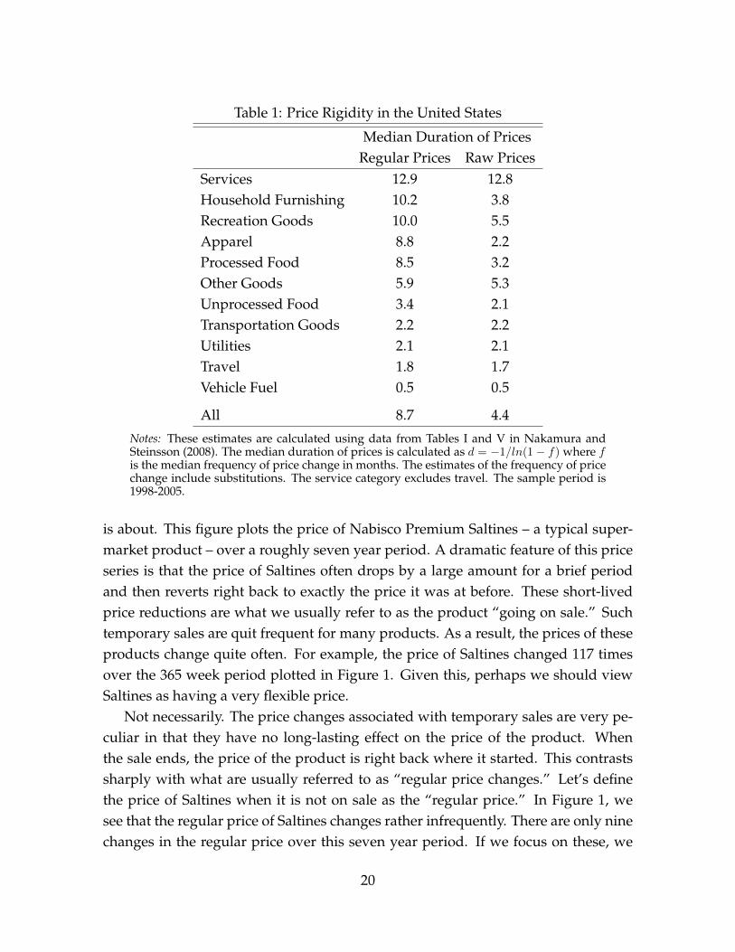
Table 1: Price Rigidity in the United States

Median Duration of PricesRegular Prices Raw Prices

Services 12.9 12.8Household Furnishing 10.2 3.8Recreation Goods 10.0 5.5Apparel 8.8 2.2Processed Food 8.5 3.2Other Goods 5.9 5.3Unprocessed Food 3.4 2.1Transportation Goods 2.2 2.2Utilities 2.1 2.1Travel 1.8 1.7Vehicle Fuel 0.5 0.5

All 8.7 4.4

Notes: These estimates are calculated using data from Tables I and V in Nakamura andSteinsson (2008). The median duration of prices is calculated as d = −1/ln(1− f) where fis the median frequency of price change in months. The estimates of the frequency of pricechange include substitutions. The service category excludes travel. The sample period is1998-2005.

is about. This figure plots the price of Nabisco Premium Saltines – a typical super-market product – over a roughly seven year period. A dramatic feature of this priceseries is that the price of Saltines often drops by a large amount for a brief periodand then reverts right back to exactly the price it was at before. These short-livedprice reductions are what we usually refer to as the product “going on sale.” Suchtemporary sales are quit frequent for many products. As a result, the prices of theseproducts change quite often. For example, the price of Saltines changed 117 timesover the 365 week period plotted in Figure 1. Given this, perhaps we should viewSaltines as having a very flexible price.

Not necessarily. The price changes associated with temporary sales are very pe-culiar in that they have no long-lasting effect on the price of the product. Whenthe sale ends, the price of the product is right back where it started. This contrastssharply with what are usually referred to as “regular price changes.” Let’s definethe price of Saltines when it is not on sale as the “regular price.” In Figure 1, wesee that the regular price of Saltines changes rather infrequently. There are only ninechanges in the regular price over this seven year period. If we focus on these, we

20

0.5

0.7

0.9

1.1

1.3

1.5

1.7

1.9

2.1

2.3

2.5

1989 1990 1991 1992 1993 1994 1995 1996 1997

Figure 1: Price of Nabisco Premium Saltines (16 oz)

Note: Price at Dominick’s Finer Food store in Chicago.

might say that the price of Saltines (that is the regular price) is quite sticky.How rigid one views prices to be, thus, depends critically on how one handles

temporary sales. What to do in this regard is somewhat controversial. However, inmy view, a strong case has been made in the literature on price rigidity that tempo-rary sales do not contribute much to the response of prices to changes in demand andcosts. This is the case for two reasons. First, prices revert quickly to their prior value,implying that temporary sales have no long-lasting effect on the level of prices. Thesecond reason is that most temporary sales occur for reasons that are unrelated todemand and costs. Arguably, most temporary sales occur for reasons of market-ing and price discrimination. Nakamura and Steinsson (2013) discuss these ideas inmore detail.

Why do firms choose not change their prices more often? Economist Alan Blinderand co-authors attempted to answer this question by simply asking firm managers(Blinder et al., 1998). When they asked the open-ended question: Why don’t youchange prices more frequently? the most common answer given by firm managerswas that they were worried about antagonizing their customers. Other frequentanswers were that they worried about competitive pressure, that changing prices iscostly, and that their costs don’t change more often.

21

Blinder and co-authors also described to the managers in plain English the logicof twelve different theories economists have proposed for price stickiness and askedthem how important these ideas were for their firm. The idea that resonated moststrongly with firm managers was that they would like to change their price but werereluctant to do this because changing their price would lead their price to get out ofline with the prices of their competitors. This is an example of a coordination failure:everyone wants to change their price, but only if everyone else does the same. Sinceeveryone is uncertain what others will do, no one changes their price.

Another idea that resonated strongly with the firm managers Blinder and co-authors surveyed was the idea of implicit contracts between firms and their customersto maintain stable prices. According to this idea, firms have an implicit understand-ing with their customers that they will not take advantage of periods of strong de-mand by raising their prices. One way to understand the logic for such implicit con-tracts is as an insurance arrangement: customers value being insured against priceincreases when demand is high. Another possible reason for implicit contracts isthat they represent a commitment by firms not to take advantage of customers whohave become partially locked into purchasing their product (e.g., because switchingto a competing product is costly).

A third idea that scored highly with the firm managers Blinder and co-authorssurveyed was the idea that it was better to adjust other product characteristics thanthe price. For example, firms might respond to an increase in demand by reducingadvertising and other sales efforts, increasing delivery lags, reducing service, or re-ducing the quality of the product. When asked why they preferred responding inthese ways, the most common answer was that they believed that these responseswere less costly and less likely to antagonize their customers.

5 Vikings Bring Back Gold Plunder

Suppose our medieval economy sends off a ship of vikings to plunder gold fromunsuspecting monasteries in neighboring countries. After their raiding is done, thevikings come home with their ship loaded to the brim with gold coins. The questionswe are interested in is how the arrival of this gold affects the medieval economy.More specifically, we would like to understand what happens to output and pricesin the medieval economy in the short run, as time passes, and in the long run.

Let’s start by considering what might happen without the aid of any equations.

22

Initially, the vikings and whoever financed their expedition are likely to go on aspending spree. They will spend some of their gold plunder on consumer goods(beer, mutton, new shoes, a new battle ax, etc.). But they may also use some of itto purchase assets (a bigger farm, more cattle, a bigger house, etc.). This spendingleads the gold they brought back to start diffusing through the economy. As thishappens, others in the economy find that they have more gold coins, which leadsthem to increase their spending as well. Before long, everyone is spending morethan before. In other words the medieval economy experiences an economic boom.

Notice that each time one person spends a gold coin another person ends upholding an extra gold coin. The people in the medieval economy are spending morethan before because they have more gold coins than before. But their spending isnot directly dissipating this situation. The extra spending is just moving the goldaround the economy. Economists often refer to this situation as one in which toomuch money is chasing too few goods.

The economic boom does, however, imply that the producers in the economyend up working more. Since the economy was in steady state before the vikingsreturned, the extra work to meet the extra demand means that the producers in theeconomy are working more than they would like. They respond to this by startingto raise their prices. As prices rise, the purchasing power of the gold coins peoplehold – their “real value” – falls, which is likely to reduce people’s desire to spend.

To summarize, this discussion conjectures that the short run response of the econ-omy to an increase in the money supply is an economic boom. The economic boomthen leads producers to start raising their prices. As prices rise, the economic boomis diminished. But where does the economy end up in the long run? The logic out-lined above suggests that prices will rise until the real value of the money supplyhas fallen back to its original value – i.e., until prices have risen by the same propor-tion as the money supply increased when the vikings brought back the extra gold.At that point, people are holding the same amount of money in real terms as beforeand therefore demand and output will be back to normal and prices will stop rising.

Let’s now see whether this description of events is what actually happens accord-ing to our medieval economy model. The first step towards this is for us to simplifythe model. Above, we defined the desired level of labor supply as L∗. We now anal-ogously define the desired level of output as the output produced with the desiredlevel of labor: Y ∗ = AL∗. We can then use this definition of Y ∗ and the productionfunction to rewrite the price setting equation – equation (4) – in terms of deviationsof output from its desired level as opposed to deviations of labor supply from its

23

desired level:Pt+1

Pt=

(YtY ∗

)θ

. (5)

With this simplification, the medieval economy model consists of only two equa-tions: 1) the price setting equation (equation (5)), and 2) the quantity equation (equa-tion (2)). (Recall that equations (1) and (2) are just two ways of writing the sameequation.) The model now has two endogenous variables: Yt and Pt. The moneysupply Mt is an exogenous variable, and the remaining parameters and variables(V , Y ∗, and θ) are also exogenously given.

5.1 Long-Run Monetary Neutrality

Let’s suppose for simplicity that no changes in the quantity of gold coins had oc-curred for a long while before the arrival of the viking ship, and the economy hadtherefore settled down to a steady state in which both prices and output were con-stant. We denote the value of each variable in this initial steady state simply byremoving its time subscript. So, steady-state output and prices before the arrival ofthe viking ship are denoted Y and P , respectively.

In this initial steady state – since prices are not changing over time – the left-hand-side of equation (5) becomes P/P = 1, which implies that the equation be-comes 1 = (Y/Y ∗)θ. Manipulation of this equation yields Y = Y ∗. In other words,output is at its desired level in the initial steady state.

Given this results, we can use the quantity equation – equation (2) – to solve forthe steady state price level prior to the arrival of the viking ship. If we denote thequantity of gold in the economy prior to the arrival of the viking ship as M , then thesteady state of the quantity equation is MV = PY . We can then plug in Y ∗ for Yand divide through by Y ∗ to get that P = MV/Y ∗. Notice that we have now solvedfor the steady state of both output and prices in terms of only exogenous variablesand parameters.

When the viking ship arrives, the money supply in our medieval economy in-creases abruptly from M to a larger value which we denote by M (M-tilde). If wewait long enough after the viking ship arrives, the economy will settle down to anew steady state. We denote the value of output and prices in this new steady stateby Y and P , respectively. The same argument as above implies that in the newsteady state Y = Y ∗ and P = MV/Y ∗.

In the long run, therefore, the extra gold has no effect on output (Y = Y = Y ∗).

24

The only effect that the extra gold has on the economy in the long run is to raiseprices. How much exactly do prices rise? We can see this by dividing the expressionfor P by the expression for P . This yields:

P

P=MV/Y ∗

MV/Y ∗ =M

M. (6)

This equation says that in the long run the price level increases by the same pro-portion as the money supply. If the amount of gold that the vikings brought backraised the money supply by 20%, equation (6) shows that the price level will even-tually also rise by 20%. When the price level has risen by the same proportion as themoney supply, the real value of the money supply is back to its original value. Wecan see this by manipulating equation (6) to yield M/P = M/P . It is at this pointthat demand for goods in the economy returns to its original value.

The results derived above are some of the most basic results in monetary eco-nomics. They are often referred to as the Classical Dichotomy or as Long-Run Mon-etary Neutrality. The Classical Dichotomy says that in the long run changes in themoney supply have no effect on “real” variables (such as output); they only affect“nominal” variables (such as the price level). The Classical Dichotomy holds in ourmedieval economy model in response to a one-time increase in the money supply.When the Classical Dichotomy holds, we say that changes in the supply of moneyare “neutral” in the long run (i.e., don’t affect real variables). We will see in chapterXX [Phillips Curve chapter] that there are ways to break the Classical Dichotomy inour simple medieval economy model.

The idea for why economists think the Classical Dichotomy should hold (or atleast should be close to holding) is that choosing the quantity of money in the econ-omy is somewhat similar to choosing a unit of measure. Just as it should not matterfor anything whether we measure weight in kilograms or pounds, it should notmatter whether we measure prices in dollars or in yen (which are worth roughly100 times less than a dollar as of this writing). If the money supply increases by afactor of 100, all prices should simply increase by a factor of 100 (in the long run)and nothing “real” should be affected.

5.2 Short Run Monetary Non-Neutrality

We now turn to the short-run effects of the arrival of the viking gold on the medievaleconomy. To analyze these effects, it is useful to take logs of the equations of the

25

model. Taking logs of the quantity equation – equation (2) – yields

logMt + log V = logPt + log Yt. (7)

(Recall that in this book log refers to the natural logarithm.) Taking logs of the pricesetting equation – equation (5) – yields

logPt+1 − logPt = θ(log Yt − log Y ∗). (8)

The medieval economy model is a dynamic model (just as the Malthus modelanalyzed in chapter XX and the Solow model analyzed in chapter XX are dynamicmodels). The price setting equation – equation (8) – is the dynamic equation in themodel, i.e., the equation that links events in different time periods. Despite beinga dynamic model, the medieval economy model is relatively simple to solve. Thesolution involves only iterating back and forth between the price setting equationand the quantity equation.

In working through these dynamics, it will prove convenient to use a version ofthe quantity equation written in terms of changes as opposed to levels. To this end,we subtract the quantity equation for time t− 1 from the quantity equation for timet. This yields

logMt − logMt−1 + log V − log V = logPt − logPt−1 + log Yt − log Yt−1

which we can write as∆ logMt = ∆ logPt + ∆ log Yt. (9)

Here we are using the symbol ∆ (Greek letter capital “delta”) to denote a “first dif-ference”, i.e., a change from one period to then next. So, for a variable logXt we havethat ∆ logXt = logXt − logXt−1. Since we are assuming that velocity is constant, itdrops out when we write the quantity equation in changes.

Let’s refer to the period in which the gold arrives as period 0. Since we are as-suming that the economy was in steady state before the gold arrives, we know thatlog Y−1 = log Y ∗, i.e., output in period -1 (the period before the gold arrives) wasequal to its desired level. We can furthermore use the quantity equation to solve forlogP−1 = logM + log V − log Y ∗, where we are using the fact that log Y−1 = log Y ∗.

Next, consider how the economy reacts at time 0, the date on which the goldarrives. Since prices in the medieval economy are set one period in advance, theywill be unchanged: At the end of period -1, price setters take stock of what happenedthat period and decide on prices for period 0. Since nothing out of the ordinary

26

happened in period -1, and output turned out to be equal to its desired level, pricesetters decide not to change their prices between period -1 and period 0. We canformally derive this by observing that the price level in period 0 is determined usingthe price setting equation – equation (8) – with t = −1:

logP0 − logP−1 = θ(log Y−1 − log Y ∗) = 0,

which implies that logP0 = logP−1.With logP0 in hand, we can use equation (9) to solve for log Y0. Equation (9) (with

t = 0) implies that∆ log Y0 = ∆ logM0 −∆ logP0.

We have seen above that ∆ logP0 = logP0 − logP−1 = 0. So, we have that ∆ log Y0 =

∆ logM0. This implies that the proportional increase in output in period 0 is equal tothe proportional increase in the money supply. (Recall that ∆ log Y0 = ∆ logM0 im-plies Y0/Y−1 = M0/M−1.) Furthermore, to a first order approximation, the percent-age change in output is equal to the percentage change in the money supply. Goingforward, we will often refer to log changes and percentage changes interchangeablywhen the changes in question are not very large.

We thus see that our medieval economy has the simple implication that, on im-pact, prices do not change and output rises by the same proportion as the moneysupply. In this sense, “the entire” increase in the money supply shows up in outputin the very short run.

Let’s now move on to period 1. The tactic we use to solve the model is the samefor period 1 and for period 0. First, we use the price setting equation (with t = 0) tosolve for logP1 given log Y0. Then we use the quantity equation (with t = 1) to solvefor log Y1 given logP1. At the end of period 0, price setters again take stock of theirsituation. Since demand was higher than its desired level in period 0, they decide toraise prices. Formally, they set

logP1 − logP0 = θ(log Y0 − log Y ∗).

Since log Y0 − log Y ∗ = ∆ log Y0 = ∆ logM0, we have that ∆ logP1 = θ∆ logM0.Armed with ∆ logP1, we can use equation (9) (with t = 1) to get that

∆ log Y1 = ∆ logM1 −∆ logP1 = −θ∆ logM0.

Here we make use of the fact that there is no change in money supply betweenperiod 0 and period 1: ∆ logM1 = 0. The level of output relative to its desired level

27

0

0.2

0.4

0.6

0.8

1

1.2

‐5 ‐4 ‐3 ‐2 ‐1 0 1 2 3 4 5 6 7 8 9 10 11 12 13 14 15 16 17 18 19 20

Log MLog PLog Y

Figure 2: Response of Medieval Economy to an Increase in the Money Supply

is

log Y1 − log Y ∗ = ∆ log Y1 + ∆ log Y0

= −θ∆ logM0 + ∆ logM0

= (1− θ)∆ logM0.

Output falls in period 1, but remains above its desired level.These derivations show that in the period after the gold arrives (t=1), prices begin

to adjust and output begins to return to its steady state. The speed of this adjustmentprocess is governed by the parameter θ, i.e., by how sticky prices are in the medievaleconomy. The stickier are prices – i.e., the smaller is θ – the slower is the adjustmentof the economy to its new steady state.

It is straightforward to continue solving for output and prices in periods 2 andbeyond. As in periods 0 and 1, this can be done by using the price setting equation tosolve for prices given output in the previous period and then by using the quantityequation to solve for output given prices. Rather than work through these steps formore periods, we present the entire path of output and prices as a function of timeafter the arrival of the viking ship in Figure 2.

In constructing Figure 2, we make specific assumptions about the exogenousvariables and parameters of the model. To make the figure as simple as possible,

28

we assume that log Y ∗ = 0, log V = 0, and logM = 0. This implies that both the log-arithm of output and the price level are equal to zero before the arrival of the vikingship. We then assume that the arrival of the viking ship raises the logarithm of themoney supply from 0 to 1, i.e., log M = 1. Finally, we set θ = 0.15.

As we had derived analytically, the initial response of the economy is for thelogarithm of output to rise by the same amount as the logarithm of the money supply(i.e., log Y0 = 1) and for the price level to remain unchanged. In subsequent periods,prices gradually rise and output gradually falls. As time passes, the logarithm ofthe price level asymptotes to one, i.e., logPt → 1 as t → ∞, and the logarithm ofoutput asymptotes to zero, i.e., log Yt → 0 as t→∞. The speed of these dynamics isgoverned by θ. Each period, prices rise θ fraction of the way they still have to go toget to one and output falls θ fraction of the way it still has to go to get to zero.

We have now seen that the arrival of the viking plunder leads to a short termboom in output. Output rises because prices are slow to adjust to the change inthe money supply. As time passes, prices gradually rise and output falls back tonormal. In the long run, output is unaffected by the viking plunder and prices arepermanently higher.

Did the arrival of the viking plunder make the people living in the medievaleconomy better off? Many people’s first reaction is to think that it did in the shortrun since output rose. This is however not correct. It is important to remember thatthe workers in the economy needed to produce the extra output. Whether peopleare better off depends on whether the extra output yields more utility than the extraeffort needed to produce that output yields disutility. In the medieval economy, wehave assumed that output is at its desired level in steady state. What the monetaryinjection does, therefore, is to raise output above its desired level. This actuallylowers people’s welfare (they wish output were lower since this would mean lesswork).

Of course, the effect of the viking plunder affects different people in the medievaleconomy differently. The vikings themselves became wealthier by plundering thegold. So, they were better off. But everyone else just worked more than they wantand were made worse off. This example illustrates well how striking gold may begood for the individual, but not necessarily good for society.

Before moving on to the next topic, let me add a little bit of nuance to the conclu-sions we came to in this section. In particular, the conclusion that a boom in outputthat results from a monetary injection reduces welfare depends critically on the as-sumption that we made above that the economy was operating at its efficient level

29

in steady state (we called it the desired level of output). There are, however, rea-sons to believe that steady state output in real world economies may be below itsefficient or desired level. If the producers in the economy have market power, theywill likely find it in their interest to set the prices of the goods they produce abovemarginal cost. This will imply that output in the economy will end up being lowerthan is efficient. In such an economy, a moderate boom in output that results froma monetary injection will raise welfare because output is temporarily brought closerto its efficient level by the boom.

6 The Price Revolution

During much of the last millennium, the unit of account throughout most of Eu-rope was defined in terms of silver and gold coins. For example, in England a silverpenny coin was minted for over a thousand years as well as various other silver andgold coins with values defined in terms of pennies, shillings, or pounds. Englandwas therefore on a specie standard – a bimetallic standard early on and later a goldstandard. Today, few currencies are on a specie standard of any kind. Some coun-tries peg their currencies to other currencies – typically the U.S. Dollar or the Euro.However, the major currencies of the world – U.S. Dollar, Euro, Japanese Yen, Chi-nese Renminbi, British Pound, etc. – are not backed by anything: they are pure fiatcurrencies.

An important potential worry with operating a fiat currency is that the value ofthe currency may not remain stable. Throughout the fiat currency era, some eco-nomic commentators as well as politicians (typically on the right of the politicalspectrum) have advocated the return to the gold standard on the grounds that thiswill prevent inflation and result in a more stable value of the currency. Over thenext few chapters, we will discuss this policy proposal several times and make useof a wide variety of evidence and theoretical ideas to assess it. We start this discus-sion here by considering the evolution of the price level in England over a 500 yearperiod from the late middle ages until right before the Industrial Revolution.

Figure 3 plots the evolution of the price level in England from 1260 to 1750. Theprice level is plotted in two different units. The gray line plots the price level inpounds sterling – the unit of account in England. The black line plots the price levelin grams of silver. Let’s begin by focusing on the gray line. A striking feature ofthe gray line is how stable it is from 1260 until 1500. For about 250 years, there

30

0

100

200

300

400

500

600

1250 1300 1350 1400 1450 1500 1550 1600 1650 1700 1750

CPI in Silver

CPI in Pounds Sterling

Figure 3: Price Level in England from 1260-1750

Note: The figure plots an estimate of the consumer price index for England from 1260 to 1750. Theblack line is consumer prices denominated in grams of silver. The gray line is consumer pricesdenominated in pence (i.e., in pounds sterling). These estimates are from Allen (2001).

was virtual price stability in England. But then something happened and pricesstarted to rise. Over the next 150 years, prices in England rose by a factor of fivebefore stabilizing and remaining relatively stable from 1650 to 1750. The evolutionof prices in other parts of Europe was similar. All countries in Europe for which dataexist experienced a large increase in prices from 1500 to 1650. The size and scope ofthis event has led economic historians to refer to it as the Price Revolution.

Clearly, being on a specie standard does not guarantee price stability: the valueof the pound sterling fell by 80% over the 16th and first half of the 17th centuries.What caused this huge increase in prices? The theoretical discussion earlier in thischapter suggests a possible explanation: Perhaps Europe experienced a major in-crease in the money supply that led prices to rise. As it turns out, Europe did infact experience a massive inflow of gold and silver (mostly silver) starting around1500. Following Columbus’ discovery of the New World in 1492, the Spanish beganimporting treasure from the Americas. Initially, they found only modest quantitiesof gold and silver. But following the discovery of rich silver deposits at Guanajuatoin Mexico and Potosi in modern day Bolivia, these imports went from being a trickle

31

0

500

1,000

1,500

2,000

2,500

3,000

3,500

4,000

1500 1520 1540 1560 1580 1600 1620 1640

Imports to Spain (Hamilton)

Production (TePaske)

Figure 4: American Treasure: Production and Imports to Spain

Note: The black line plots Hamilton’s (1934) estimates of imports of gold and silver to Spain fromthe Americas by decade from 1500 to 1660. Hamilton reports these in pesos (450 maravedıs). I haveconverted them into metric tons of silver assuming that each maravedıs is 0.094g of silver. The grayline plots TePaske’s (2010) estimates of production of gold and silver in the New World by decadefrom 1500 to 1660. TePaske reports these in pesos (272 maravedıs). I have also converted these intometric tons of silver assuming that each maravedıs is 0.094g of silver.

to a flood.Figure 4 plots estimates of Spain’s imports of American treasure from 1500 to

1660 by Hamilton (1934) as well as estimates of production of gold and silver inthe Americas by TePaske (2010). Most American gold and silver reached Europethrough Spain over this period. The import and production measures plotted in Fig-ure 4 differ for several reasons. First, both estimates are subject to error since sourcesare imperfect. Second, some gold and silver was used as money in the Americas andsome was exported to Asia. These shares were small initially but grew over time.Third, Hamilton’s estimates may understate imports to Spain due to illicit smug-gling.

These imports of gold and silver from the New World constituted a huge mone-tary shock for Europe. The stock of gold and silver in Europe prior to 1492 is difficultto estimate. But a rough estimate by Glassman and Redish (1985) indicates that thecombined value of gold and silver money in Europe in 1492 was equal to the value

32

of 3,541 metric tons of silver.1 The estimates in Figure 4 indicate that around 1600imports to Europe of gold and silver every 15-20 years where larger than the entirepre-1492 stock of monetary gold and silver on the continent. No wonder prices rose.In fact, it may seem puzzling that prices didn’t rise even more. An important rea-son for this is that Western Europeans reexported a large amount of gold and silverto the Baltic, the Levant, and Asia to finance imports of goods from these areas. Infact a large share of all imports to Europe from Asia were financed with silver andgold rather than with the sale of European goods in Asia. For example, over 2/3 ofthe exports of the British East India Company to Asia was precious metals between1660 and 1700 (Cipolla, 1976/1993, p. 220). The gold and silver that entered Eu-rope through Spain, thus, didn’t only flow to other countries in Western Europe butflowed all over the Old World.

The coincidence in the timing of the Price Revolution and the massive flow ofgold and silver into Europe strongly supports the notion that the Price Revolutionwas caused by the inflow of gold and silver from America in the 16th and 17th cen-turies. In light of this, it is perhaps surprising how controversial this explanationhas been. Both contemporaries and later scholars have proposed a myriad of otherexplanation for the sharp rise in prices in 16th and 17th century Europe. The mostprominent alternative explanations pin the rise in prices on monopolists and mid-dlemen, population increases, and high demand from abroad.

The idea that inflation is caused by monopolists and middlemen that raise pricesby engrossing, forestalling, and regrating—to use Hamilton’s (1934) language—is acommon theme across time and space. However, this idea is flawed. Monopolistsand middlemen can raise the price of the goods they sell relative to the prices ofother goods. They cannot raise the overall level of all prices. Someone may object:What if there are monopolists and middlemen selling all products? Won’t that makethe price of all products high? But high relative to what?

Perhaps monopolists and middlemen make prices high relative to wages. Thisis in fact possible. But this is not what happened over the course of the Price Rev-olution. Both prices and wages rose by large amounts in Europe from 1500 to 1650.Such a general increase in both prices and wages cannot be explained by the nefari-ous actions of monopolists and middlemen.

It is true that real wages—i.e., wages relative to prices—in England fell between1500 and 1650 (see Figure 2 in chapter XX [Malthus chapter]). Adherents of themonopolists and middlemen view can point to these movements as evidence sup-porting their thesis. But several objections can be raised against this argument. First,

33

chapter XX [Malthus chapter] provides an alternative explanation for the fall in realwages between 1500 and 1650 based on Malthusian population dynamics. Second,the fall in real wages may be interpreted as evidence that monetary expansions canlower real wages in cases where real wages are initially stuck at levels that are “toohigh”—i.e., above market-clearing levels. Third, it is not clear why monopolists andmiddlemen became so much more problematic during the period 1500-1650 than inother periods. What is really special about this period of time is the huge inflow ofsilver (and gold).

The idea that population increase caused the Price Revolution is also flawed. Itis an application of the Malthusian ideas discussed in chapter XX [Malthus chapter].The basic idea is that larger populations increased demand for food and therebydrove up food prices. But again, this is an argument about one price relative to an-other, not an argument about the general increase in all prices. As we discussed inchapter XX [Malthus chapter], increases in the population will result in lower realwages in a Malthusian economy (i.e., the price of food rising relative to wages). Pop-ulation pressure can therefore explain the fall in real wages over the period 1500 to1650, but not the large increase in the overall prices level (including nominal wages).

The idea that the Price Revolution was caused by excessive demand from abroadis less flawed. Our medieval economy model implies that increases in the moneysupply result in high demand in the short run. This demand does not particularlycome from abroad. But contemporary complaints about excessive foreign demandmay simply have been due to tribalism and political posturing. This explanation,however, leaves open the question why demand rose. The monetary theory of thePrice Revolution provides an explanation for this: demand rose because of the sharpincrease in the money supply.

One of the oldest surviving formulations of the quantity theory of money thatunderlies our medieval model is by the French scholar Jean Bodin in the context of adebate about the causes of the Price Revolution (Bodin, 1568). Bodin was respondingto an explanation put forth by Sieur de Malestroit that the increase in prices experi-enced in France at the time was due to civil unrest, bad harvests, loss of labor afterfamines, and bullion exports (de Malestroit, 1566)—an early example of confusionabout the causes of inflation which has been and remains very common. Even ear-lier discussions of the quantity theory have survived by the French scholar Oresmefrom around 1350, the Polish scholar Copernicus from around 1520, and membersof the School of Salamanca in Spain in the 16th century. It seems likely that manyprior scholars formulated some version of the quantity theory, but that records of

34

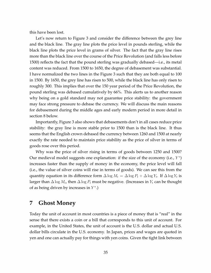
this have been lost.Let’s now return to Figure 3 and consider the difference between the grey line

and the black line. The gray line plots the price level in pounds sterling, while theblack line plots the price level in grams of silver. The fact that the gray line risesmore than the black line over the course of the Price Revolution (and falls less before1500) reflects the fact that the pound sterling was gradually debased—i.e., its metalcontent was reduced. From 1500 to 1650, the degree of debasement was substantial.I have normalized the two lines in the Figure 3 such that they are both equal to 100in 1500. By 1650, the grey line has risen to 500, while the black line has only risen toroughly 300. This implies that over the 150 year period of the Price Revolution, thepound sterling was debased cumulatively by 66%. This alerts us to another reasonwhy being on a gold standard may not guarantee price stability: the governmentmay face strong pressure to debase the currency. We will discuss the main reasonsfor debasement during the middle ages and early modern period in more detail insection 8 below.

Importantly, Figure 3 also shows that debasements don’t in all cases reduce pricestability: the gray line is more stable prior to 1500 than is the black line. It thusseems that the English crown debased the currency between 1260 and 1500 at nearlyexactly the rate needed to maintain price stability as the price of silver in terms ofgoods rose over this period.

Why was the price of silver rising in terms of goods between 1250 and 1500?Our medieval model suggests one explanation: if the size of the economy (i.e., Y ∗)increases faster than the supply of money in the economy, the price level will fall(i.e., the value of silver coins will rise in terms of goods). We can see this from thequantity equation in its difference form ∆ logMt = ∆ logPt + ∆ log Yt. If ∆ log Yt islarger than ∆ logMt, then ∆ logPt must be negative. (Increases in Yt can be thoughtof as being driven by increases in Y ∗.)

7 Ghost Money

Today the unit of account in most countries is a piece of money that is “real” in thesense that there exists a coin or a bill that corresponds to this unit of account. Forexample, in the United States, the unit of account is the U.S. dollar and actual U.S.dollar bills circulate in the U.S. economy. In Japan, prices and wages are quoted inyen and one can actually pay for things with yen coins. Given the tight link between

35

the units of account that exist today and actual coins and bills, it is tempting to thinkthat this is how things must be, i.e., that the unit of account is bound to correspondto the physical money circulating in a particular economy.

But this is not at all so. In fact, historically, the unit of account has often deviatedfrom the coins and bills circulating in economies in ways that at first may appearquite strange. Cipolla (1956) gives a classic account of this:

For centuries the people of Western Europe went on using monetaryterms such as libra (pound), solidus (shilling), denarius (penny), and flo-renus (florin) in fixing the prices of their commodities and services, inestablishing any sort of debts, or in keeping accounts. Everybody usedthose terms and carried on transactions in them ... Yet, and here the mys-tery begins, during the greatest part of the Middle Ages and the firstcenturies of the modern period, with the exception of a few short peri-ods, nobody ever saw many of those “moneys” about which everybodytalked. For instance, nobody for centuries ever saw a real pound, for thesimple, but paradoxical, reason that the pound during the greatest partof its life did not materialize into a real, visible, and touchable coin. Itwas a ghost money. (page 38)

An important lesson from monetary history is that the unit of account can livea life of its own quite independent of the coins and bills circulating in the economy(and other mediums of exchange). The history of units of account in Western Europeover the past 2000 years illustrates this clearly.

We start this story with the monetary system of the late Roman Empire. From thefourth century C.E., this was based on the solidus, a gold coin that weighed roughly4.5 grams. The solidus continued to be minted by the Byzantine Empire after thefall of Rome and was the dominant coin used in Mediterranean trade until the endof the 7th century. The Muslim conquests of the 7th and 8th century substantiallyaltered the balance of power in the Mediterranean and gave rise to a rival coin: themuslim dinar. The dinar was the result of a monetary reform instituted by Calif AbdAl-Malik ibn Marwan in the 690s. From that time until the thirteenth century, thesolidus (also called the nomisma) and the dinar were together dominant coins forinternational trade in the Mediterranean.

The disintegration of the Western Roman Empire in the 5th century C.E. resultedin significant regress in monetary matters in Western Europe for some time. Coinsbecame scarce. Obligations were often settled in kind rather than with coins. The

36

units of account continued to be concepts such as solidi and denarii, which cor-responded to coins that existed or had existed. But the medium of exchange inmost transactions were everyday commodities (or labor). In this sense, the economyshifted closer to a barter economy, but one with coin-based units of account.

An important change occurred in the eight century when the Carolingian kingPepin the Short reformed the monetary system of the Carolingian Empire (soon tobecome the Holy Roman Empire). His son Charlemagne finalized these reforms inthe 790s. The new system—which became the dominant monetary system in West-ern Europe—was based on a silver penny (denarius in Latin or denier in French)weighing about 1.7 grams. This penny was the only coin minted in Western Europefor several hundred years.

The most prevalent unit of account prior to these reforms was the solidus(shilling in English or sou in French). The value of a solidus at the time was roughlyequal to twelve of the new pennies. To link the new system with the old system, theCarolingian reform declared a solidus (shilling) to be equal to twelve pennies. Fi-nally, the weight of the penny was determined such that 240 pennies could be struckfrom a pound (libra in Latin or livre in French) of silver.

The Carolingian monetary system was therefore based on three units:

1 pound = 20 shillings = 240 pennies.

Only one of these three units corresponded to a real coin (the penny). The shillingwas the name of an old coin used to link the old and the new monetary systems.The pound was not a coin either. It was originally a unit of weight of silver. Thissomewhat odd monetary system consisting of dozens and scores of dozens was re-markably long lived. It was only in 1795 that France replaced this system with adecimal system (1 franc equal to 100 centime). The last country to use this monetarysystem was Britain, which only switched to a decimal system in 1971.

The Carolingian penny was a relatively modest monetary unit. It was a conve-nient unit for many everyday transactions. But for larger transaction such as whole-sale merchant transactions, it was a small unit. Merchants therefore found it usefulto record trades in pounds and shillings. Cipolla (1956, p. 41) discusses how ini-tially pounds referred to the weight of the silver involved in a transaction, but overtime pounds came to mean simply “240 pennies.” Similarly, solidus (shilling) re-ferred initially to the gold coin of that name, but over time came to mean simply “12pennies.”

This distinction was not material at first, but for reasons discussed in detail in

37

section 8, the penny was progressively debased over time, i.e., its silver content wasreduced. This process meant that as time passed the amount of silver in 240 penniesfell below 1 pound by greater and greater amounts. At that point there arose a con-flict between the monetary unit “1 pound” and the pound as a measure of weight.It is not obvious what should happen in such a circumstance. Some might think itmore natural that the monetary unit “1 pound” remain equal to 1 pound of silverand that its exchange rate with the penny should simply have varied as the pennywas debased. But this is not what happened. The pound as a unit of account cameto live a life of its own independent of its original meaning as the weight of somenumber of pennies.

The same is true of the solidus (shilling). Originally, the gold solidus coin wasequal in value to 12 pennies. As pennies were debased, the gold solidus coin came tobe worth more than 12 pennies. However, the solidus as a unit of account remained12 pennies. In monetary matters, it was therefore important to distinguish betweenthe unit of account “1 solidus” and the actual gold solidus coin, which was worthmore than 12 pennies. As with the pound, the ghost money had begun to live a lifeof its own.

In the 12th and 13th centuries, various states in Western Europe began mintingnew coins representing denominations larger than the penny. The florin minted inFlorence from 1252 onward and later the ducat minted in Venice became importantcoins in Mediterranean trade. The gold florin was originally equivalent to 240 lo-cal pennies. It therefore materialized the local pound. In France Louis IX issues agold half-pound coin (initially worth 120 pennies) as well as a silver shilling worth12 pennies. However, “that happy moment when the ghosts materialized and letthemselves be touched and seen by everybody did not last for a long time” Cipolla(1956, p. 43) explains. Generally, the penny was debased more than the larger goldcoins resulting in the value of the gold coins rising relative to the penny as timepassed. As this happened, “the ghosts left their material features and began againtheir mysterious, invisible life” (ibid).

The story of the Milanese florin as told by Cipolla (1956, p. 46-47) drives thepoint home. The Milanese florin was rated at 120 pennies when it was first struckin 1252. However, as the penny was debased its value rose. By 1340 it was worth384 pennies. At that point, the debasement of the penny seized for some time andthe exchange rate between the florin of Milan and the local penny remained stablefor about 60 years. Over this period, the people of Milan came to use the florin as anadditional unit of account. The system of denominations in Milan towards the end

38

of the 14th century therefore had four denominations:

1 florin = 1.6 pounds = 32 shillings = 384 pennies

1 pound = 20 shillings = 240 pennies

1 shilling = 12 pennies

Two of these units were ghosts (the pound and the shilling) and two were actualcoins (the florin and the penny). In the fifteenth century, the debasement of thepenny relative to the florin resumed. But by this point, the practice of using theflorin as a unit of account was sufficiently ingrained—for example in accountingpractices—in Milan that the Milanese simply continued to use the term “florin” tomean 384 pennies, just as they used the term “pound” to refer to 240 pennies eventhough 240 pennies were no longer equal to 1 pound of silver. The florin as a unitof account became a ghost, i.e., an abstract monetary unit. The value of the actualgold florin coin rose over time relative to this abstract florin. By 1445, a gold florincoin was worth about 768 pennies. In other words, 1 “real” gold florin was worth 2“ghost” florins.

Cipolla (1956) gives several other examples. The Genoese came to use the term“florin” as an abstract unit of account equal to 300 pennies (25 shillings) even as theGenoese gold florin became worth more than this. The Venicians came to use theterm “ducat” similarly to mean 124 shillings irrespective of the value of the actualgold Venician ducat. It was universally the case that the term shilling meant 12 andpound meant 240. But florin meant different things in different cities, as did otherunits.

This discussion suggests that contemporary merchants (as well as later day schol-ars) had to contend with a rather complicated monetary system during the MiddleAges. It seems likely that all this complexity was costly in various ways and there-fore detrimental to trade: those not sufficiently knowledgeable could be tricked;contracts might be open to several interpretations unless monetary matters werespelled out in great detail (e.g., did the term “florin” as used in the contract meanthe gold coin of that name or the abstract monetary unit). What prevented the mone-tary authorities of this era from instituting a simpler and more transparent monetarysystem? We take up this question in the next section.

39

8 The Big Problem of Small Change

During the decades prior to World War I, most countries in the world were on agold standard. Many accounts of monetary history begin with this classical goldstandard period, proceed to discuss its downfall, and then detail the tumultuoushistory of monetary arrangements over the 20th century. This narrative can givethe false impression that all of history prior to 1914 was characterized by a goldstandard. In fact, despite its great fame, the classical gold standard period was verybrief: it lasted only from the 1870s until 1914.

In chapter XX, we discuss the reasons for the downfall of the gold standard. Here,however, we consider why the gold standard didn’t emerge earlier. A central chal-lenge faced by monetary authorities for many centuries—and arguably the reasonwhy the gold standard did not emerge earlier—was how to maintain coins of differ-ent value in circulation simultaneously. Recall that prior to bills, bank deposits, andother modern media of exchange, coins were the main medium of exchange in soci-ety. Coins of vastly different value where needed for the simple reason that the scaleof transactions varied enormously. On the one hand, low-value coins were neededfor everyday household transactions. On the other hand, high-value coins wereneeded for large-scale transactions such as wholesale transactions of merchants. Aswe will see below, monetary authorities faced particularly severe problems in pro-viding for low-value coins—providing for small change. This challenge is some-times referred to as the “big problem of small change” (Cipolla, 1956; Sargent andVelde, 2002).

Practical considerations implied upper and lower limits on the size of coins. Onthe one hand, very large coins were too easy to counterfeit, for example, by fillingthe interior with a base metal (Redish, 2000, p. 19). Bodin (1606/1962, p. 689) arguedthat 31g was a rough upper limit. On the other hand, coins could not be so smallthat they were easily lost or difficult to pick up and count. Bodin argued that coinssmaller than 1.3g were difficult to stamp and too brittle. The smallest denominationEnglish coins in the 15th century, where actually quite a bit smaller than this. Thefarthing (1/4 of a penny) weighed only about 0.25g at this time (Redish, 2000, p.109). For comparison, a U.S. dime is 2.27g and a euro 1 cent coin is 2.3g.

Clearly, the farthing, the halfpenny, and even the penny were extremely smallcoins in the 15th century. Yet, the value of these coins was not at all trivial from thepoint of view of everyday transactions. Allen (2001) estimates that the day wage ofbuilding laborers in London in 1425 was 5d (i.e., 5 pence). A penny was therefore

40

20% of a day’s wages for a building laborer and the tiny farthing was 5% of a day’swages for such a worker. For comparison consider a worker in 2020 who made $15per hour and worked an 8 hour day. 20% of such a worker’s daily wages was $24,while 5% was $6. This means that the smallest denomination silver coin in Englandin the 15th century was to a building laborer of that time roughly comparable to a$5 bill in 2020.

Conducting everyday transactions with a $5 bill as the smallest denominationseems cumbersome enough. But the situation was actually worse than this sincethere was a chronic shortage of farthings and halfpennies. Minting such tiny coinswas expensive (relative to their modest value). While sovereigns may have paidsome attention to the public service aspect of keeping small coins in circulation, theyalso put considerable weight on the profits minting generated. For this or some otherreason, they failed to enact policies that resulted in adequate supply of farthings andhalfpennies (Redish, 2000, p. 108-115). In many cases, therefore it is likely that thesmallest coins available in the 15th century in England were pennies. Imagine howcumbersome everyday transactions would be if the smallest denomination of moneywas a $24 coin (at 2020 prices).

The fundamental difficulty monetary authorities faced in the 15th century in pro-viding an efficient medium of exchange was that “silver—an object of intermediatevalue—was too valuable to provide a medium of exchange for the smallest transac-tions and too cheap to use for high-value transactions” as economic historian AngelaRedish put it in her excellent book on bimetallism which this section draws on heav-ily (Redish, 2000, p. 19). One solution for small transactions was to mint coins ofvarying fineness, i.e., coins made of an alloy of silver and copper with a smallershare of silver than “sterling silver” coins which contained 92.5% silver (or at sometimes 91.67%). Such coins were called “billon” in France and “vellon” in Spain. Bil-lon coins were never minted in England.

An important drawback of billon coins was that it was difficult—even for skilledassay-masters—to assess their fineness (Redish, 2000, p 21-24). This resulted instrong incentives to counterfeit billon coins, i.e. mint replicas of official coins withlower silver content than the official coins. Also, different polities on the continentof Europe would mint very similar deniers (pennies) and would each have an incen-tive to lower slightly the proportion of silver in the deniers they minted relative toexisting deniers in circulation. This would allow them to offer better prices for thecoins they minted than competing polities. Over time, this led to very substantialdebasement of the denier on the continent. England was spared this dynamic by

41

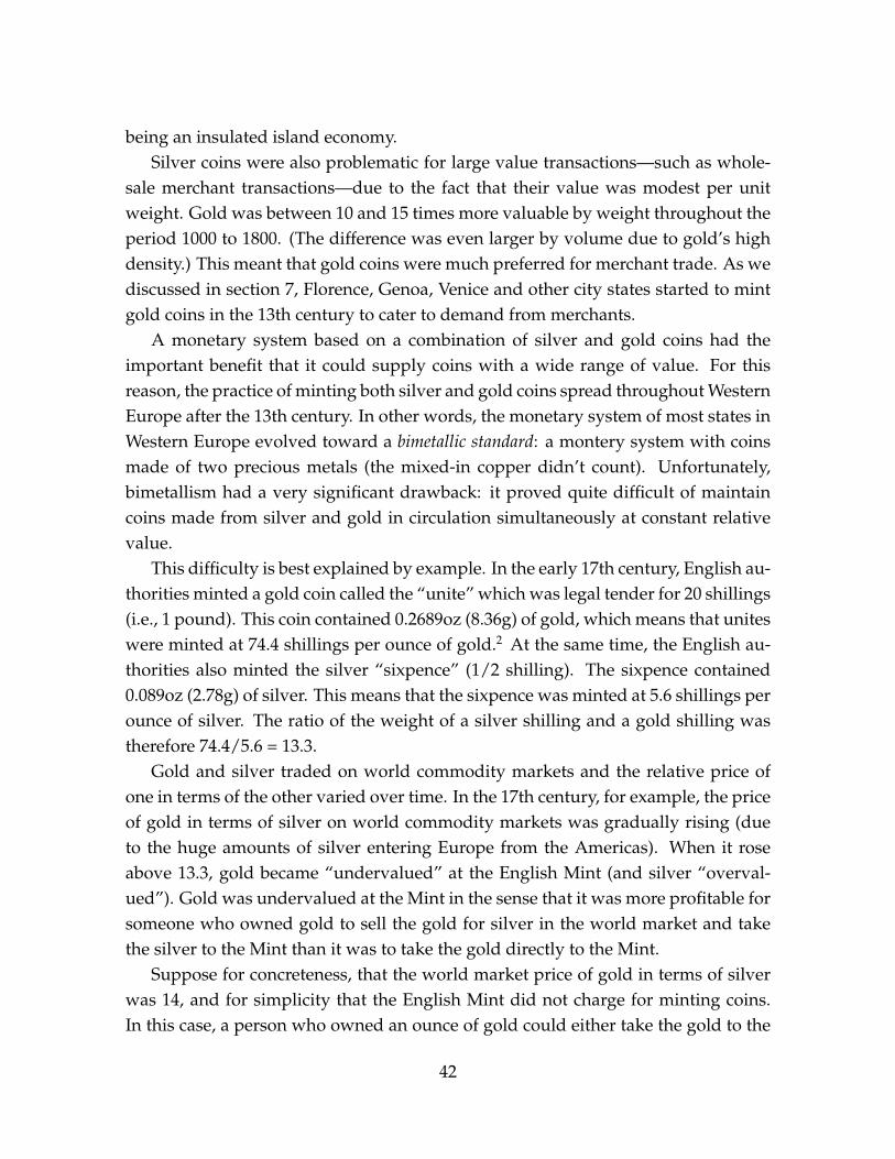
being an insulated island economy.Silver coins were also problematic for large value transactions—such as whole-

sale merchant transactions—due to the fact that their value was modest per unitweight. Gold was between 10 and 15 times more valuable by weight throughout theperiod 1000 to 1800. (The difference was even larger by volume due to gold’s highdensity.) This meant that gold coins were much preferred for merchant trade. As wediscussed in section 7, Florence, Genoa, Venice and other city states started to mintgold coins in the 13th century to cater to demand from merchants.

A monetary system based on a combination of silver and gold coins had theimportant benefit that it could supply coins with a wide range of value. For thisreason, the practice of minting both silver and gold coins spread throughout WesternEurope after the 13th century. In other words, the monetary system of most states inWestern Europe evolved toward a bimetallic standard: a montery system with coinsmade of two precious metals (the mixed-in copper didn’t count). Unfortunately,bimetallism had a very significant drawback: it proved quite difficult of maintaincoins made from silver and gold in circulation simultaneously at constant relativevalue.

This difficulty is best explained by example. In the early 17th century, English au-thorities minted a gold coin called the “unite” which was legal tender for 20 shillings(i.e., 1 pound). This coin contained 0.2689oz (8.36g) of gold, which means that uniteswere minted at 74.4 shillings per ounce of gold.2 At the same time, the English au-thorities also minted the silver “sixpence” (1/2 shilling). The sixpence contained0.089oz (2.78g) of silver. This means that the sixpence was minted at 5.6 shillings perounce of silver. The ratio of the weight of a silver shilling and a gold shilling wastherefore 74.4/5.6 = 13.3.

Gold and silver traded on world commodity markets and the relative price ofone in terms of the other varied over time. In the 17th century, for example, the priceof gold in terms of silver on world commodity markets was gradually rising (dueto the huge amounts of silver entering Europe from the Americas). When it roseabove 13.3, gold became “undervalued” at the English Mint (and silver “overval-ued”). Gold was undervalued at the Mint in the sense that it was more profitable forsomeone who owned gold to sell the gold for silver in the world market and takethe silver to the Mint than it was to take the gold directly to the Mint.

Suppose for concreteness, that the world market price of gold in terms of silverwas 14, and for simplicity that the English Mint did not charge for minting coins.In this case, a person who owned an ounce of gold could either take the gold to the

42

Mint and receive 74.4 shillings or sell the ounce of gold for 14 ounces of silver on theworld market, take this silver to the Mint and receive 14× 5.6 = 78.4 shillings.

In this situation, no one would mint gold coins. If the difference between theprice of gold in terms of silver at the Mint and in world markets was large enough,it might even become profitable to melt down gold coins, sell the gold in worldmarkets for silver, and take that silver to the Mint. Such a situation would eventuallylead to only silver coins circulating with the adverse consequences for trade that thisentails.

In reality, transaction costs meant that gold and silver coins could circulate alongside each other even when the gold-silver price ratio at the Mint differed from thegold-silver price ratio in the world market by a non-trivial amount. One type oftransaction cost was the fee the Mint charged, i.e., the gross seignorage. For example,a person presenting gold to the English Mint in 1615 received unite coins worth only72 shillings per ounce even though 74.4 shillings worth of such coins were mintedper ounce. The Mint kept the remaining 2.4 shillings per ounce as seignorage. (TheMint also charged seignorage for minting silver coins.) In addition to seignorage,melting coins, shipping gold abroad for sale, and reimporting silver entailed signif-icant costs. These costs implied that arbitraging differences in the gold-silver priceratio at the Mint versus in world commodity markets was only profitable when thisdifference was quite substantial.

A second problem that led to undervalued coins was wear from circulation andclipping. Normal use of a coin leads the coin to gradually loose some of its weight.For gold and silver coins, this can be substantial over longer periods of time. Inaddition, “clippers” would profit from clipping small amounts of silver off of coins,collecting these clippings, melting them down, and selling them as bullion.

Wear from circulation and clipping implied that older coins were lighter thannewly issued coins. If older coins continued to circulate “by tale” (i.e., by number)as opposed to by weight, this meant that newly issued coins were undervalued atthe Mint relative to the older coins. For everyday household transactions, weighingcoins every time they transact would be very cumbersome. In practice, therefore lowvalue coins generally circulated by tale. But this meant that people had an incentiveto pay with older lighter coins rather than newer heavier coins. Heavier coins tendedto be exported or melted down. This is another example of Gresham’s Law: badmoney drives out good money. In this case, the worn out (lighter) coins are “badmoney”, while the newer (heavier) coins are “good money”.

Over time, the difference in weight between older worn out coins and newly

43

issued coins would cause a shortage of official coins and a proliferation of counterfeitcoins as well as foreign imitation coins. These counterfeit and foreign imitation coinsbecame cheaper to produce than official coins as the stock of coins in circulationbecame more and more worn (and therefore lighter). The price of silver in the worldcommodity market would rise above what people could get by bringing silver to theRoyal Mint. Once this had happened, very few new official coins would be mintedunless the monetary authorities were willing to subsidize the minting of additionalofficial coins. This whole process would lead the stock of coins in circulation tobecome more and more heterogeneous, which risked undermining the efficiency ofthe coins as a medium of exchange. As a result, complaints about the state of thecoinage would multiply (Feavearyear, 1963, p. 10-20).

These problems were arguably a primary reason for debasement of low valuecoins in England and other Western European countries after the 14th century. Facedwith a stock of coins in greater and greater disarray, monetary authorities would pe-riodically choose to realign the silver content of newly issued coins with those incirculation by reducing the weight of newly issued coins, i.e., debase the currency.This would encourage people to bring silver to the Mint and discourage counter-feiting. The difference between the black line and the gray line in Figure 3 reflectsthis process of gradual debasement of the currency. Evidently, wear and clipping ofcoins was another reason—in addition to increases in the supply of silver—why be-ing on a commodity standard did not guarantee price stability in the late medievaland early modern period.

Sometimes coins would be debased not for the reasons discussed above, but toraise revenue. Debasement allowed states to raise their seignorage rates temporar-ily and also increase the quantity of coins minted (older coins often lost their legaltender status). For both of these reasons, debasements were a source of revenue forthe state. Such debasement was however unpopular. States therefore refrained fromsuch debasements except when their fiscal needs were dire (e.g., during wars). Fis-cal debasements were also less frequent in states with stronger institutions, wherefiscal needs could be met in other ways.

There are also instances when the states decided to recall coins in circulationand recoin without depreciating the currency. One instance of this is the Englishrecoinage of 1696. In such a case, the holders of the worn coins bore the cost. Theyhad taken a light coin as payment for (say) a shilling when its true silver contentwas only 9d (9 pence). They must then return the coin to the Mint in exchangefor for 9d worth of newly issued coins. In the case of the recoinage of 1696, the

44

English Exchequer (treasury) offered to purchase worn and clipped coins prior tothe recoinage and therefore bore most of the fiscal cost of the recoinage.

Today, our monetary system no longer suffers from the “big problem of smallchange.” The reason for this is that an effective solution to this problem was eventu-ally devised. The solution was to issue token coins: coins that have a monetary valueabove the value of the metal they are made of. This system is now universally usedby monetary authorities to supply low value coins. But despite its simplicity, it tookcenturies to work out. It was only in 1816 that England first adopted this system,and other nations adopted it still later (e.g., the United States in 1853 and France in1865).

Why did it take so long for the big problem of small change to be solved? Onereason was surely the widespread metallist fallacy that money must be backed by anobject that has non-monetary value (such as gold or silver). Our discussion of stonemoney on the island of Yap earlier in the chapter, not to mention the near universaluse of fiat money for the last 50 years has clearly demonstrated that money need notbe backed by items with non-monetary value. But this belief was clearly widely helduntil not so long ago and may have clouded the thinking of monetary authorities.

Another reason emphasized by Redish (1990, 2000) was technological. The factthat the face value of a token coin was higher than the value of the metal the coinwas made of created potential for profitable counterfeiting. For example, if 5s 6d (5shillings and 6 pence) were coined from an ounce of silver when the price of silver onthe market was only 5s, counterfeiters could earn a profit as long as their costs werelower than 6d per ounce. (Their profits would be 6d minus their cost per ounce.) Ifcounterfeiting was not very costly, this would place a tight bound on the differencebetween the face value of a token coin and the value of the metal it was made of.

The traditional technology for making coins was by hammering blanks: a blankwas placed between two dies and the top was struck several times with a hammer.This method created coins of uneven size and quality. Such coins were easily coun-terfeit. In the 17th century, this method was replaced by a fly-press and the edges ofthe coins were milled or engraved. The fly-press created somewhat more uniformcoins. But the major advantage of this method was that the milled or engraved edgesmade clippings more obvious and therefore discouraged clipping of coins.

Redish (1990, 2000) argues that it was not until the advent of steam power in theearly 19th century that coins could be made with sufficient uniformity and qualityto substantially raise the costs of counterfeiting. Steam power was first adapted tominting by Matthew Boulton (James Watt’s partner). Between 1805 and 1811, the

45

Royal Mint was fitted with Boulton’s machines. In addition to producing coins ofsuperior quality, Boulton’s machines had the advantage of being an expensive pro-prietary technology that was hard for counterfeiters to replicate. These technologicalchanges removed a crucial impediment to the adoption of token coins.

Ever since Sir Isaac Newton, as Master of the Mint, overvalued gold coins inEngland in 1717, very little silver coinage had been minted in England. This led to asevere shortage of small denomination coins throughout the 18th century. The silvershillings and sixpence that did circulate became extremely worn as the century woreon. By 1798, shillings in circulation had lost 25% of their weight and sixpence 38%(Redish, 2000, p. 142). This sorry state of affairs eventually led to reform of the silvercoinage in England. The Coinage Act of 1816 called for new silver coins to replacethe old. Significantly, these new silver coins would be token coins: 5s 6d would beminted from an ounce of silver, whereas the market price of silver at the time was5s. The Act ended “free coinage” of silver—i.e., the notion that anyone could bringsilver to the Mint for coining. This meant that Britain had shifted from an officialbimetallic standard to a gold standard.

Ending free coinage of silver was crucial. Since the face value of token coins ishigher than the metal they are made of, it is profitable to create them. This meansthat their supply must be controlled. If anyone had been allowed to exchange silverbullion for such coins in arbitrary quantity the Mint would have been flooded withsilver and the price of the coins would eventually have been driven down to thevalue of the metal they were made of. Reflecting the rather foggy understanding theEnglish authorities had of the reform they were undertaking, it was somewhat bylucky happenstance that the Coinage Act did not include a clause allowing for freecoinage of silver (Redish, 2000, p. 148-149).

Another crucial feature of a successful monetary system based on token coins isthat the monetary authority must commit to redeem the token coins at face value.Without this guarantee, the value of the token coins will not necessarily remain equalto their face value and, in particular, might well fall towards the value of the metalthey are made of. The importance of this type of convertibility was another aspect ofthe reform that seems not to have been well understood by the English authoritiesinitially. In this case, it was the Bank of England—at the time a private for-profitinstitution—that helped make the new token silver coins a success by guarantee-ing their convertibility into gold coins at par. Eventually, a confrontation betweenthe Bank and the Exchequer forced the Exchequer to take on the responsibility ofguaranteeing convertibility.

46

The coinage system Britain adopted in 1816 proved to be the solution to all theproblems discussed in this section. It constitutes a major advance in monetary prac-tice and was eventually universally adopted. The crucial element of the “standardformula” Britain devised was the issue of token subsidiary coins that were freelyconvertible at par and of sufficiently high quality that counterfeiting was not prof-itable. This system allowed monetary authorities to issue coins with a wide rangeof values without difficulty. Actually, this system allowed monetary authorities tocompletely stop thinking about the composition of the money supply across denom-inations. (The Fed doesn’t care how much of the money supply is nickels versusquarters.) With the big problem of small change solved, the focus of monetary pol-icy shifted from providing an efficient medium of exchange to maintaining stableprices.

9 The Crime of 1873

In the U.S. presidential election of 1896, William Jennings Bryan was the candidateof the Democratic party. The U.S. was on the gold standard by this point. It hadundergone the transition from a traditional bimetallic standard with its “big problemof small change” to the standard formula with token low value coins discussed insection 8 earlier in the 19th century. However, Bryan’s principle campaign issue was“free silver” at “16 to 1”—that is, a return to a bimetallic standard. By 1896, theCoinage Act of 1873, which demonetized silver—and thereby shifted the U.S. from abimetallic standard to a gold standard—was by many considered a “grave wrong,”a “conspiracy,” a “great legislative fraud,” or simply “the crime of 1873” (Barnett,1964; Friedman, 1990b).

William McKinley was Bryan’s Republican opponent. He ran on a platform ofremaining on the gold standard. Even though Bryan ran a memorable campaignthat included one of the most famous convention speeches of all time in which hethundered “You shall not press down upon the brow of labor this crown of thorns,you shall not crucify mankind upon a cross of gold”, Bryan lost the election by avote margin of 4.3 percent (and an electoral college margin of 271 to 176).

Given all the problems associated with being on a bimetallic standard discussedin section 8, it may seem surprising that Bryan’s central campaign issue was thereturn to a bimetallic standard. Also, why did Bryan argue that being on a goldstandard was a “crown of thorns” for labor? Furthermore, why were technical mat-

47

ters of monetary policy so central in a presidential election campaign during theclassical gold standard period? Isn’t that period held up as a golden era of monetarystability? Why all this agitation about monetary matters during that era?

Answering these questions is not merely of historical interest. It helps us un-derstand key challenges associated with being on a gold standard (or any speciestandard, for that matter). As in section 6, we will see that when countries are ona specie standard their macroeconomic outcomes are at the mercy of unpredictablevariation in the supply of bullion.

The Coinage Act of 1792 defined the dollar as the basic monetary unit of theUnited States. According to the act, the dollar was equal to 371.25 grains (24.06g)of pure silver or 24.75 grains (1.60g) of pure gold. The act authorized free coinageof both gold and silver. Coinage was free in two senses of the word: first, anyonecould take bullion to the mint in unlimited amounts and receive coins in exchange;second, coinage was free of charge, i.e., the mint did not charge seignorage.

The Coinage Act of 1792 thus placed the United States on a bimetallic standardwith a gold-silver price ratio of 15 to 1. The principle architect of the Act was trea-sury secretary Alexander Hamilton. Hamilton had recommended the ratio of 15 to1 because this was the prevailing market rate at the time the act was being drafted.Hamilton’s hope was that both gold and silver coins would circulate in the U.S.and the U.S. economy would thus benefit from an efficient medium of exchange fortransactions over a wide range of values (Redish, 2000, p. 212-213).

Hamilton’s hopes in this regard were thwarted by the fact that the market priceof gold in terms of silver rose shortly after 1792 and remained above 15 thereafter.We can see this in Figure 5, which plots the price of gold in terms of silver from 1690to 1870. The fact that the market price of gold in terms of silver was above 15 after1792 meant that gold was undervalued at the U.S. mint and silver was overvalued.The public therefore brought silver to the U.S. Mint rather than gold and the U.S.was effectively on silver standard.

In the early 19th century, there was considerable debate in the U.S. about themonetary standard. Some argued that the absence of gold coins was detrimental tocommerce, while others argued that the use of bank notes—which was more com-mon in the U.S. than in other countries at the time—was an effective substitute forhigh denomination coins. Several committees recommended raising the gold-silverprice ratio at the mint to a value closer to the prevailing market price of gold withmost discussion centering on a value of 15.625. In 1834, legislation was introducedto raise the gold-silver price ratio to 15.625. Shortly before the legislation passed,

48

13.5

14.0

14.5

15.0

15.5

16.0

16.5

1690 1710 1730 1750 1770 1790 1810 1830 1850 1870

Figure 5: Gold-Silver Price Ratio, 1690-1870

Note: The figure plots the gold-silver price ratio (ounces of silver for an ounce of gold). The sourceis Officer and Williamson (2021). The construction of this series is described in Officer (Undated-b).

however, the price ratio was changed to 16. Why this was done is not entirely clear,but it was likely due to political considerations. President Andrew Jackson was atthe time engaged in a battle to eliminate the Second Bank of the United States. Somethink that raising the price ratio to 16 was done to undermine the Bank by encour-aging the minting of gold coins as a substitute for bank notes issued by the Bank.Others have argued that the higher price ratio was chosen to benefit gold producingstates (Friedman, 1990, Redish, 2000, p. 216-224).

The passage of the Coinage Act of 1834 meant that silver became undervaluedat the Mint and gold overvalued. At first, the degree of undervaluation of silverwas small (see Figure 5). During this period silver continued to circulate and someadditional silver coins were minted (although much more gold coins were minted).Following the California gold rush (which began in 1848), the price of gold fell andsilver became more substantially undervalued at the Mint. This led silver coins to bewithdrawn from circulation (exported or melted down)—an example of Gresham’sLaw and the “big problem of small change” (Redish, 2000, p. 227-232).

Congress in the U.S. responded to the growing shortage of small denominationcoins by passing legislation in 1853 that reduced the silver content of subsidiary

49

silver coins (those with a face value less than $1). This change made subsidiarysilver coins in the U.S. into token coins and thus took an important step towardseliminating the big problem of small change. However, the 1853 legislation did notrequire the Treasury to redeem these coins and thus did not fully anchor their marketvalue at their face value. A commitment to redeem subsidiary silver coins did notbecome law in the U.S. until 1879.

The outbreak of the Civil War in 1861 resulted in an enormous increase in govern-ment spending. Financing this spending was a huge challenge. One of the responsesof the Union government to this challenge was to issue paper currency—so called“greenbacks.” The Union government printed large quantities of these greenbacksand used them to pay for the war effort. Greenbacks were not backed by gold orsilver and no explicit promise was made to redeem them in gold or silver. Gold andsilver coins continued to circulate as well, but not at a 1-to-1 exchange rate. TheUnion economy, thus, effectively had a dual monetary system during the Civil Warwith both greenbacks and gold coins serving as money at a floating exchange rate.Greenbacks were the dominant form of money in most of the country, but gold coinswere also widely used for certain purposes, particularly on the west coast.

As the war progressed and more and more greenbacks were issued, their valuefell. In other words, there was a large amount of inflation. Figure 6 plots the evolu-tion of the price level in the U.S. between 1825 and 1914 with the price level in 1860normalized to 100. The figure shows that over the course of the War, the price level(in greenbacks) roughly doubled.

After the war, there was a widespread desire in the financial community (andgenerally among those in the country with political power) to return to a speciestandard—a system of “sound money.” This was accomplished with a sequence ofacts of Congress in the 1870s. An important consideration was at what exchangerate greenback dollars should be made convertible into gold. Adopting a gold stan-dard at the pre-War exchange rate entailed reducing the price level by a very largeamount—i.e., raising the price of the greenback dollar up to the price of the old golddollar by reversing much of the inflation of the war years. The alternative was to fixthe dollar at a lower exchange rate (fewer dollars per ounce of gold). We will dis-cuss the economics of this choice in more detail in chapter XX. The final decision—embodied in the Resumption Act of 1875—was to adopt the pre-War exchange rate.Resumption was scheduled for January 1, 1879 and was successfully executed at thattime.

Our focus in this section is, however, the Coinage Act of 1873. This act listed the

50

50

75

100

125

150

175

200

225

1825 1835 1845 1855 1865 1875 1885 1895 1905

Figure 6: An Estimate of the Consumer Price Index in the U.S., 1825-1914

Note: The figure plots an estimate of the evolution of the consumer price index in the United Statesfrom 1825 to 1914. The price level in 1860 is normalized to 100. The source is Williamson (2021). Theconstruction of this series is described in detail in Officer (Undated-a). It uses series constructed byDavid and Solar (1977), Rees (1961), Douglas (1930), as well as the Bureau of Labor Statistics.

coins to be minted in the U.S. going forward. It included gold coins and token silvercoins. However, it ended free coinage of the silver dollar. This effectively movedthe U.S. from a bimetallic standard to a gold standard, just as the British CoinageAct of 1816 had done in Britain. The adoption of token subsidiary silver coins hadremoved the traditional rationale for being on a bimetallic standard. So, the U.S.adopted Britain’s “standard formula.” The Act was passed by an overwhelmingmajority in both houses of Congress and attracted little attention at the time it waspassed.

At roughly the same time (i.e., in the 1870s), Germany switched from a silver-based currency to a gold standard, as did France. France had operated a bimetallicmonetary system with a gold-silver price ratio of 15.5 from 1803. This likely playedin important role in stabilizing the gold-silver price ratio despite substantial golddiscoveries in California and Australia around 1850 (Friedman, 1990a). The nearsimultaneous demonitization of silver in France, Germany, and the United States inthe 1870s constituted a huge negative shock to the demand for silver. As a result, theprice of silver began to fall relative to gold.

51

0

5

10

15

20

25

30

35

40

45

1800 1810 1820 1830 1840 1850 1860 1870 1880 1890 1900 1910

Figure 7: Gold-Silver Price Ratio, 1800-1914

Note: The figure plots the gold-silver price ratio (ounces of silver for an ounce of gold). The sourceis Officer and Williamson (2021). The construction of this series is described in Officer (Undated-b).

Figure 7 plots the price of gold in terms of silver between 1800 and 1914. Theprice ratio was very stable between 15 and 16 from 1800 until the 1870s. During the1870s, it started to rise. By 1880 it had risen to 18 and in the 1880s it rose to 22. Thisincrease in the price of gold in terms of silver implied that, if not for the Coinage Actof 1873, the U.S. would have resumed convertibility to specie in 1879 on a de factosilver standard as opposed to a gold standard: silver would have been overvalued atthe mint and gold undervalued leading the public to bring silver to the mint ratherthan gold.

Why does this matter? It matters primarily because of its effect on the price level.Countries on the gold standard experienced a persistent, large deflation (fall in theprice level) during the 1870s, 1880s, and early 1890s. Figure 8 plots the price levelin the U.S. and Britain from 1870 to 1914. Between 1875 and 1895, the price level inboth countries trended downward. Cumulatively, the price level fell by 23% in theU.S. and 18% in Britain over this period. In the mid-1890s, however, the price levelin both the U.S. and Britain stopped falling and then began to rise. From that pointuntil the beginning of World War I, these countries (and other countries on the goldstandard) experienced persistent inflation rather than persistent deflation.

52

70

80

90

100

110

120

130

140

1870 1875 1880 1885 1890 1895 1900 1905 1910

United States

Britain

Figure 8: An Estimate of the Consumer Price Index in the U.S. and Britain, 1870-1914

Note: The figure plots an estimate of the evolution of the consumer price index in the United Statesand Britain from 1870 to 1914 (1913 in the case of Britain). Both series are normalized to 100 in 1879.The sources are the same as for Figures 3 and 6.

For the United States, the deflation between 1875 and 1895 was a continuation ofa much larger deflation that began with the end of the Civil War (see Figure 6). Aswe discussed above, the U.S. decided to adopt a gold standard at the pre-Civil Warexchange rate between the dollar and gold. This entailed raising the value of thegreenback dollar—equivalently, reducing the price level—by a very large amount.The large deflation between 1865 and the mid-1870s was primarily caused by thispolicy.

In contrast, the deflation between 1875 and 1895 was a global phenomenon af-fecting all gold standard countries. Its cause likely lies in the supply and demandfor gold. In particular, the demand for gold increased substantially over this periodfor two reasons. First, countries representing a substantial fraction of world GDPadopted the gold standard and, thus, demanded large quantities of gold to backtheir money supply. (The money supply was rapidly switching from metal coins topaper notes during this period. We will discuss this in more detail in chapter XX[Money and Banking Chapter].) Second, the world economy expanded at a rapidclip during this period as millions of Europeans emigrated to the New World and

53

the Industrial Revolution spread to larger and larger parts of the world.To understand the effect that these developments had on the price level in gold

standard countries, it is useful to refer back to the model that we developed in sec-tions 4 and 5. The quantity equation implies that

∆ logMt = ∆ logPt + ∆ log Yt. (10)

(See discussion on page 26.) Rearranging this equation, we get

∆ logPt = ∆ logMt −∆ log Yt. (11)

The logic for this equation is that changes in the price level are determined by thebalance between two factors: 1) changes in the supply of money ∆ logMt, whichare heavily influenced by changes in the quantity of gold (i.e., gold mining), and2) changes in the demand for money, which are determined in our simple modelby ∆ log Yt. If the supply of money increases faster than the demand for money,prices will rise. If, however, the demand for money increases faster than the supplyof money, prices will fall. During the period 1875 to 1895, mining of gold—whileconsiderable—did not keep up with the rapid increase in the demand for gold formonetary purposes. As a result, the price level in countries on the gold standard fellpersistently.

You may again ask: Why does this matter? Why, in particular, did the publicget sufficiently exercised about this deflation for it to be a major campaign issue ina presidential election? One reason is that changes in the price level affect the realvalue of debt contracts. Debt contracts are typically written in nominal terms (e.g.,in dollars). When the price level falls, the real value of debts rises. This is goodfor creditors, but bad for debtors. Debtors, therefore, typically do not like deflation,while creditors do not like inflation (which erodes the real value of debt contracts).

This idea is perhaps best grasped through an example. Consider a farmer whotakes out a $1,000 loan (a considerable sum in the 1870s) to build a barn, buy live-stock, or otherwise improve his or her farm. Suppose for simplicity that the farmermust pay 5% in interest per year and repay the principle at the end of a 5 year term.If the price level falls by (say) 10% over this 5 year period—as occurred (roughlyspeaking) in the mid-1870s and again in the mid-1880s—the amount the farmer mustrepay measured in terms of goods is 10% higher than it was when he took out theloan. The prices of the farmer’s own output are likely to have fallen by roughlythis same amount over the period of the loan. The farmer must then sell 10% morewheat, corn, cotton, or whatever else he or she produces to be able to pay off the

54

loan, a considerable burden. In reality, agricultural prices fell by more than prices ingeneral in the 1870s and 1880s, adding further to the plight of indebted farmers.

For these reasons, indebted farmers in the 1880s and 1890s were susceptible topropaganda about a “crime of 1873” perpetrated by eastern and foreign capitalists(“Wall Street”) to demonetize silver so as to raise the value of their loans at the ex-pense of the public (“Main Street”). Others, who didn’t believe that a literal crimehad been committed, also came to see the Coinage Act of 1873 as a “grave wrong” interms of its economic consequences. William Jennings Bryan’s campaign to restore“free silver” at “16 to 1” was about reversing this wrong. His goal was to end thepersistent deflation the U.S. had experienced over the prior 30 years and bring aboutinflation to ease the burdens of indebted farmers.

Other related ideas likely also factored in Bryan’s thinking. “Tight money” poli-cies tend to depress output in the short run, as prices respond sluggishly to increasedmoney demand. This occurs for reasons similar to those that produced the boom inoutput in response to the arrival of the viking gold in section 5. Bryan may haveunderstood this at some level and wanted to reverse it.

The idea of restoring free coinage of silver at a price ratio of 16 to 1 was by manyconsidered a thoroughly irresponsible proposal in 1896. At the time, the gold-silverprice ratio was roughly 30 to 1. Opponents argued that Bryan’s policies would resultin runaway inflation. A naive view was that the price level would roughly double,to reflect the low market price of silver. This, however, failed to take account of thefact that if the U.S. were to restore free coinage of silver at 16 to 1, the price of silverwould have risen substantially.

It is not out of the question that the price of silver in terms of gold would haverisen all the way to 16. After all, France had managed to stabilize the gold-silverprice ratio in the vicinity of 15.5 from 1803 until the 1870s. Perhaps the U.S. couldhave done the same at the turn of the 20th century. In that case, the effect of adoptingbimetallism in 1896 at 16 to 1 would have been modest. Friedman (1990b) argues,however, that a more likely outcome would have been a price ratio of about 24 in1896 if Bryan had been elected (see also Friedman, 1992, ch. 4). In this case, Bryan’selection would have resulted in considerable inflation.

Curiously, despite Bryan losing the election of 1896, the deflation he sought toend did in fact end around that time. In the late 1890s, the price level reached bottomand gradually started to rise (see Figure 8). As a consequence, Bryan’s populistmovement lost considerable steam and Bryan lost the presidential elections of 1900and 1908 by wider margins than the election of 1896. The cause of the turnaround

55

in the price level is pretty obvious. The world production of gold skyrocketed in the1890s. In the 1880s, about 50 tons of gold where mined annually in the world. Thisrose to roughly 130 tons in the period 1900-1914 (Eichengreen and McLean, 1994).

This huge increase in gold production was made possible by two roughly con-temporaneous developments. First, vast gold fields were discovered in South Africaaround this time. Second, a commercially viable process was developed to extractgold from the low-grade ore in these gold fields—the so-called cyanide process.So, it came to pass that William Jennings Bryan’s chances of becoming president ofthe United States were undone by Scottish chemists and South African miners. Ofcourse, the only reason why this could happen was that the workings of the mone-tary system of the United States at the time was subject to the vagaries of the globalgold-mining industry.

Scholars who advocated bimetallism in the late 19th century (and 20th century)did so because they thought that bimetallism was likely to result in more stableprices than a monometallic system (such as a gold standard or silver standard). Thisrepresented a sharp break from earlier analysis of bimetallism. Prior to the 19thcentury, the primary rationale for bimetallism had been providing for an efficientmedium of exchange (the big problem of small change discussed in section 8). Butby the mid-19th century, this problem had been solved and price stability had be-come the paramount concern of monetary scholars. (Later scholars have sometimesscoffed at the idea that considerations of small change could drive the nature of themonetary system (Friedman, 1990a, p. 99-100).)

A bimetallic standard can result in a more stable price level than a monometallicstandard because the second metal can add elasticity to the supply of money incases where there is substantial mismatch between changes in money demand andchanges in the supply of the first metal. Friedman (1990b) makes this case for theperiod 1875 to 1895. In particular, he argues that the U.S. would have been betterserved if the Coinage Act of 1873 had not omitted free coinage of silver. In thatcase, the U.S. would have resumed specie payments in 1879 on the basis of silver, asopposed to gold. This would have resulted in less world demand for gold over thesubsequent decades and more world demand for silver. As a result the price level ingold standard countries would have fallen less and the price level in silver standardcountries increased by less. Friedman argues that the price level in the United Stateswould have been more stable over the period 1875 to 1914 in this case than it wasin actuality. However, he stresses that this is a judgment about 1873, not 1896. By1896, when Williams Jennings Bryan ran for president on a free-silver ticket, it was

56

too late. The damage of omitting silver in 1873 had already been done and could notbe undone. As Friedman puts it: “Bryan was trying to close the barn door after thehorse had been stolen.”

57

Notes1Glassman and Redish (1985, p. 40) average two earlier estimates of the stock of money in Europe

in 1492 from King (1696) and Del Mar (1877). The average is 15.1 million marcs argent-le-roi. Theyexplain that 1 pound sterling is 0.4548 marcs and 1,718 troy grains of pure silver. One troy grainis equal to 0.0647989 grams. Marcs being argent-le-roi means that they are 23/24 pure silver. Wetherefore have 15.1× 1, 718× (1/0.4548)× 0.06479× (23/24) = 3, 541.

Velde and Weber (2000) estimate the value of the world stock of gold and silver in 1492 to beequal to the value of 6,900 metric tons of silver. They estimate the world stock of silver in 1492 to be3,600 metric tons and the world stock of gold to be 297 metric tons. I use a price of gold in terms ofsilver of 11 to calculate the value of the stock of gold in terms of silver.

2The unite weighted 140.8 troy grains of 11/12 fine gold. Each troy grain is 0.0647989g. Each troyounce is 480 grains. See Redish (2000, p. 27-28).

References

ALLEN, R. C. (2001): “The Great Divergence in Wages and Prices from the MiddleAges to the First World War,” Explorations in Economic History, 38, 411–447.

BARNETT, P. S. (1964): “The Crime of 1873 Re-examined,” Agricultural History, 38.

BLINDER, A. S., E. R. CANETTI, D. E. LEBOW, AND J. B. RUDD (1998): Asking AboutPrices, New York, NY: Russell Sage Foundation.

BODIN, J. (1568): La Response de Maistre Jean Bodin, advocat en la Cour, au Paradoxe deMonsieur de Malestroit touchant l’encherissement de totes hoses et le moyen d’y remedier,Paris.

——— (1606/1962): The Six Bookes of a Commonweale, Cambridge, MA: Harvard Uni-versity Press.

BUDISH, E. (2018): “The Economic Limits of Bitcoin and the Blockchain,” WorkingPaper, University of Chicago.

CIPOLLA, C. M. (1956): Money, Prices, and Civilization in the Mediterranean World:Fifth to Seventeenth Century, Princeton, NJ: Princeton University Press.

——— (1976/1993): Before the Industrial Revolution: European Society and Economy1000-1700 (Third Edition), New York, NY: W.W. Norton & Co.

DAVID, P. A. AND P. SOLAR (1977): “A Bicentenary Contribution to the History ofthe Cost of Living in America,” 2, 1–80.

DE MALESTROIT, S. (1566): Les Paradoxes du Seigneur de Malestroit, conseillor du Roiet Maistre ordinaire de ses comptes, sur le faict des Monnoyes presented a Sa Majeste’ aumois de Mars MDLXVI, Paris.

DEL MAR, A. (1877): “Minute on the World’s Production of Gold and Silver,” in Re-

58

port of the U.S. Monetary Commission, Washington, DC: U.S. Government PrintingOffice.

DOUGLAS, P. H. (1930): Real Wages in the United States, 1890-1926, Boston, MA:Houghton.

EICHENGREEN, B. AND I. W. MCLEAN (1994): “The Supply of Gold under the Pre-1914 Gold Standard,” Economic History Review, 47, 288–309.

FEAVEARYEAR, A. (1963): The Pound Sterling, Oxford, UK: Oxford University Press.

FRIEDMAN, M. (1990a): “Bimetallism Revisited,” Journal of Economic Perspectives, 4,85–104.

——— (1990b): “The Crime of 1873,” Journal of Political Economy, 98, 1159–1194.

——— (1992): Monetary Mischief, New York, NY: Harcourt Brace & Company.

FURNESS, H. W. (1910): The Island of Stone Money: Uap and The Carolines, Philadel-phia, PA: J.B. Lippincott Co.

GLASSMAN, D. AND A. REDISH (1985): “New Estimates of the Money Stock inFrance, 1493-1680,” Journal of Economic History, 45, 31–46.

HAMILTON, E. J. (1934): American Treasure and the Price Revolution in Spain, 1501-1650, Cambridge, MA: Harvard University Press.

KING, G. (1696): King, Natural and Political Observations and Conclusions upon the Stateand Condition of England, London, UK.

NAKAMURA, E. AND J. STEINSSON (2008): “Five Facts about Prices: A Reevaluationof Menu Cost Models,” Quarterly Journal of Economics, 123, 1415–1464.

——— (2013): “Price Rigidity: Microeconomic Evidence and Macroeconomic Impli-cations,” Annual Review of Economics, 5, 133–163.

OFFICER, L. H. (Undated-a): “What Was the Consumer Price Index Then? A DataStudy,” MeasuringWorth, http://www.measuringworth.com/uscpi/.

——— (Undated-b): “What Was the Price of Gold Then? A Data Study,” Measuring-Worth, http://www.measuringworth.com/uscpi/.

OFFICER, L. H. AND S. H. WILLIAMSON (2021): “The Price of Gold, 1257-Present,”MeasuringWorth, http://www.measuringworth.com/gold/.

PIAZZESI, M. AND M. SCHNEIDER (2018): “Payments, Credit, and Asset Prices,”Working Paper, Stanford University.

REDISH, A. (1990): “The Evolution of the Gold Standard in England,” Journal ofEconomic History, 50, 789–805.

——— (2000): Bimetallism, Cambridge, UK: Cambridge University Press.

REES, A. (1961): Real Wages in Manufacturing, 1890-1914, Princeton, NJ: PrincetonUniversity Press.

59

SARGENT, T. J. AND F. R. VELDE (2002): The Big Problem of Small Change, Princeton,NJ: Princeton University Press.

SMITH, A. (1776/2000): An Inquiry into the Nature and Causes of the Wealth of Nations,New York, NY: The Modern Library.

SWEENEY, J. AND R. J. SWEENEY (1977): “Monetary Theory and the Great CapitolHill Baby Sitting Co-op Crisis,” Journal of Money, Credit and Banking, 9, 86–89.

TEPASKE, J. J. (2010): A New World of Gold and Silver, Leiden, The Netherlands:Koninklijke Brill NV.

VELDE, F. R. AND W. E. WEBER (2000): “A Model of Bimetallism,” Journal of PoliticalEconomy, 108, 1210–1234.

WALTER, J. R. (1989): “Monetary Aggregates: A User’s Guide,” Federal ReserveBank of Richmond, Economic Review, Jan/Feb 1989.

WILLIAMSON, S. H. (2021): “The Annual Consumer Price In-dex for the United States, 1774-Present,” MeasuringWorth,http://www.measuringworth.com/uscpi/.

60