Money Illusion and Housing Frenzies∗

Markus K. Brunnermeier†

Department of EconomicsPrinceton University

Christian Julliard‡

Department of EconomicsLondon School of Economics

this version: July 24, 2006

AbstractA reduction in inflation can fuel run-ups in housing prices if people suffer

from money illusion. For example, investors who decide whether to rent or buya house by simply comparing monthly rent and mortgage payments do not takeinto account that inflation lowers future real mortgage costs. We decompose theprice-rent ratio in a rational component — meant to capture the proxy effect andrisk premia — and an implied mispricing. We find that inflation and nominalinterest rates explain a large share of the time-series variation of the mispricing,and that the tilt effect is very unlikely to rationalize this finding.

Keywords: Housing, Real Estate, Inflation, Inflation Illusion, Mortgages, Behav-ioral FinanceJEL classification: G12, R2.

∗We benefited from helpful comments from an anonymous referee, Yakov Amihud, Patrick Bolton,Smita Brunnermeier, John Campbell, James Choi, Albina Danilova, Aureo de Paula, Emir Emi-ray, Will Goetzmann, Kevin Lansing, Chris Mayer, Alex Michaelides, Stefan Nagel, Martin Oehmke,Maureen O’Hara (the editor), Filippos Papakonstantinou, Lasse Pedersen, Adriano Rampini, MattRichardson, Bob Shiller, Matt Spiegel, Jeremy Stein, Demosthenes Tambakis, Haibin Zhu and sem-inar and conference participants at the Bank of England, Cambridge-Princeton conference, CSEF-IGIER symposium, Duke-UNC Asset Pricing Conference, 2006 Econometric Society Winter Meet-ings in Boston, Federal Reserve Bank of Philadelphia, Harvard University, IIES Stockholm, LondonBusiness School, London School of Economics, NBER Behavioral Meetings, Oxford University, Queen-Mary University, RFS Bubble Conference in Indiana, University of Copenhagen, University of Salerno,Wharton School, University of Wisconsin-Madison Real Estate Research conference, and Yale Con-ference on Behavioral Economics. We also thank the BIS for providing part of the housing data usedin this analysis. Brunnermeier acknowledges financial support from the National Science Foundationand the Alfred P. Sloan Foundation.

†Princeton University, Department of Economics, Bendheim Center for Finance, Princeton, NJ08544-1021, NBER and CEPR, e-mail: markus@princeton.edu, http://www.princeton.edu/∼markus

‡Department of Economics, London School of Economics, Houghton Street, London WC2A 2AE,United Kingdom, and CEPR, e-mail: C.Julliard@lse.ac.uk, http://personal.lse.ac.uk/julliard/

1

1 Introduction

Housing prices have reached unprecedented heights in recent years. Sharp run-upsfollowed by busts are a common feature of the time-series of housing prices. Figure1 illustrates different real housing price indices and shows that this phenomenon hasbeen observed in several OECD countries.

US UK CA A U

P a n e l A

1970 1974 1978 1982 1986 1990 1994 1998 200250

75

100

125

150

175

200

225

250

275

NLS E

DKCH

NO

Panel B

1970 1974 1978 1982 1986 1990 1994 1998 200250

75

100

125

150

175

200

225

250

275

Figure 1: Residential property (real) price indices for a group of Anglo-Saxon countries(Panel A) and for Scandinavian countries and other European countries (Panel B). Baseperiod is 1976:Q1.

Shiller (2005) documents similar patterns for other countries and cities over shortersamples. Moreover, Case and Shiller (1989, 1990) document that housing price changesare predictable and suggest that this might be due to inefficiency in the housing mar-ket. There are several potential reasons for this market inefficiency — one of thembeing money illusion. The housing market is particularly well suited to study moneyillusion, since frictions make it difficult for professional investors to arbitrage possiblemispricings away.In this paper we identify an empirical proxy for the mispricing in the housing market

and show that it is largely explained by movements in inflation. Inflation matters andit matters in a particular way. Our analysis shows that a reduction in inflation cangenerate substantial increases in housing prices in a setting in which agents are proneto money illusion. For example, people who simply base the decision of whether torent or buy a house on a comparison between monthly rent and monthly payment of

2

a fixed nominal interest rate mortgage suffer from money illusion. They mistakenlyassume that real and nominal interest rates move in lockstep. Hence, they wronglyattribute a decrease in inflation to a decline in the real interest rate and consequentlyunderestimate the real cost of future mortgage payments. Therefore, they cause anupward pressure on housing prices when inflation declines.To identify whether the link between housing price movements and inflation is due

to money illusion, we first have to isolate the rational components of price changes thatare due to movements in fundamentals such as land and construction costs, housingquality, property taxes, and demographics (Mankiw and Weil (1989)).1 We do so intwo stages. First, we focus on the price-rent ratio to insulate our analysis from fun-damental movements that affect housing prices and rents symmetrically. Even thoughrenting and buying a house are not perfect substitutes, the price-rent ratio implicitlycontrols for movements in the underlying service flow. Second, we try to isolate rationalchannels through which inflation could influence the price-rent ratio. Several authorsincluding Fama (1981) have claimed that the negative relationship between inflationand the price of real assets (like stocks) might be due to a “proxy effect”: high inflationand/or high inflation expectations are a bad signal about future economic conditions.Moreover, higher inflation might make the economy more risky or agents more riskaverse, generating a risk premium that is correlated with inflation. Also, an increasein inflation reduces the after-tax user cost of housing, potentially driving up hous-ing demand (Poterba (1984)). We use a Campbell and Shiller (1988) decompositionthat takes into account housing specific risk factors, (such as probability of movinginteracted with cross-sectional variation of house prices), to decompose the price-rentratio into rational components (expected future returns on housing investment andrent growth rates) and a mispricing component. After controlling for rational chan-nels, we find that inflation has substantial explanatory power for the sharp run-upsand downturns of the housing market.Figure 2 depicts the time series of the (estimated) mispricing component of the

price-rent ratio in the U.K. housing market and its fitted values obtained using inflationas the only explanatory variable. The first thing to notice is that the mispricing showssharp and persistent run-ups during the sample period. Moreover, the fitted seriesclosely tracks the mispricing.

The close link between inflation and housing prices could be due to a departurefrom rationality and/or financing frictions. First, as argued by Modigliani and Cohn(1979), if agents suffer from money illusion, their valuation of an asset will be inverselyrelated to the overall level of inflation in the economy. This explanation of housing

1These variables alone are generally not able to capture the sharp run-ups in housing prices. It hasbecome common in the empirical literature to add cubic ‘frenzy’ terms in the housing price regressions(see Hendry (1984) and Muellbauer and Murphy (1997)) and the rational expectations hypothesis hasbeen rejected by the data (Clayton (1996)).

3

MISPRICING FITTED_INFSM

1967 1971 1975 1979 1983 1987 1991 1995 1999 2003-0.15

-0.10

-0.05

0.00

0.05

0.10

0.15

Figure 2: Mispricing and fitted series based on U.K. inflation

price run-ups would also be in line with the finding of McCarthy and Peach (2004)that the sharp run-up in the U.S. housing market since the late 1990s can be largelyexplained by taking into account the contemporaneous reduction of nominal mortgagecosts. A special form of money illusion arises if home owners are averse to realizingnominal losses. Second, in an inflationary environment, the nominal payments on afixed-payment mortgage are higher by a factor that is roughly proportional to thereciprocal of the nominal interest rate. This causes the real financing cost to shifttowards the early periods of the mortgage, therefore causing a potential reduction inhousing demand and prices. This is the so called tilt effect of inflation (see Lessardand Modigliani (1975) and Tucker (1975)). Nevertheless, why the tilt effect shouldmatter cannot be fully explained in a rational setting since financial instruments thatare immune to changes in inflation, like the price level adjusted mortgage (PLAM) orthe graduate payment mortgage (GPM), have been available to house buyers since atleast the 1970s. Most importantly, in Section 4.1 we perform a series of tests whichmake it seem very unlikely that the tilt effect is the driving force of the empiricallink between inflation and housing prices. Third, if fixed interest rate mortgages arenot portable, individuals that have bought a house and have locked in a low nominalinterest rate might be less willing to sell their current house to buy a better one when

4

nominal interest rates are higher. Hence, an increase in inflation that raises the nominalinterest rate might depress the price of better-quality residential properties. On theother hand, a reduction in inflation and nominal interest rates would free current homeowners from this “lock-in” effect. We provide evidence that the “lock-in” effect is notdriving our results. Further, we show that housing supply elasticity is heterogeneousacross U.S. states due to differences in population density. We show that given thisheterogeneity in supply elasticity, money illusion can lead to heterogeneous regionalprice dynamics as observed in the data.The balance of the paper is organized as follows. The next section reviews the

related literature on money illusion, market frictions and speculative trading. Section3 formally analyzes the link between inflation and housing prices using the U.K. housingmarket as a case study.2 In particular, Subsection 3.1 provides a first assessment ofthe empirical link between price-rent ratio and inflation. Subsection 3.2 decomposesthe price-rent ratio isolating the rational channels from an estimated mispricing andshows that the mispricing is largely explained by changes in the rate of inflation.Section 4 argues that market frictions — like the tilt effect (Subsection 4.1) and lock-ineffect (Subsection 4.2) — are unlikely to be the cause of the link between inflation andmispricing on the housing market. Section 5 confirms our main empirical results usingU.S. data and studies the heterogeneity of housing supply elasticity across the U.S. Afinal section concludes and a full description of the data sources, methodological detailsand additional robustness checks are provided in the appendix.

2 Related Literature

2.1 Money Illusion and Psychological Biases

“An economic theorist can, of course, commit no greater crime than toassume money illusion.” Tobin (1972)

“In fact, I am persuadable — indeed, pretty much persuaded — that moneyillusion is a fact of life.” Blinder (2000)

In this section we sketch the links to the existing literature. In particular, wereview previous definitions of money illusion, relate it to the psychology literature andsummarize the empirical evidence on the effect of money illusion on the stock market.

Definition of Money Illusion. Fisher (1928, p. 4) defines money illusion as “thefailure to perceive that the dollar, or any other unit of money, expands or shrinks in

2We first focus on the U.K. market since the better quality of the housing data, the longer sampleperiod in housing prices (1966:Q2—2004:Q4) and inflation linked bonds (1982:Q1-2004:Q4), the avail-ability of PLAM and GPM mortgage schemes, and the fact that most U.K. mortgages are portable,allow for sharper and more robust inference.

5

value.”3 Patinkin (1965, p. 22) refers to money illusion as any deviation from decisionmaking in purely real terms: “An individual will be said to be suffering from such anillusion if his excess-demand functions for commodities do not depend [...] solely onrelative prices and real wealth...” Leontief (1936) is more formal in his definition byarguing that there is no money illusion if demand and supply functions are homogeneousof degree zero in all nominal prices.

Related Psychological Biases. Money illusion is also very closely related to otherpsychological judgement and decision biases. In a perfect world money is a veil andonly real prices matter. Individuals face the same situation after doubling all nominalprices and wages.The framing effect states that alternative representations (framing) of the same

decision problem can lead to substantially different behavior (Tversky and Kahneman(1981)). Shafir, Diamond, and Tversky (1997) document that agents’ preferences de-pend to a large degree on whether the problem is phrased in real terms or nominalterms. This framing effect has implications on (i) time preferences as well as on (ii)risk attitudes. For example, if the problem is phrased in nominal terms, agents preferthe nominally less risky option to the alternative which is less risky in real terms. Thatis, they avoid nominal risk rather than real risk. If on the other hand the problem isstated in real terms, their preference ranking reverses. The degree to which individualsignore real terms depends on the relative saliency of the nominal versus real frame.Anchoring is a special form of framing effect. It refers to the phenomenon that

people tend to be unduly influenced by some arbitrary quantities when presented witha decision problem. This is the case even when the quantity is clearly uninformative.For example, the nominal purchasing price of a house can serve as an anchor for areference price even when the real price can be easily derived.4 Genesove and Mayer(2001) document that investors are reluctant to realize nominal losses.While individuals understand well that inflation increases the prices of goods they

buy, they often overlook inflation effects which work through indirect channels, e.g.general equilibrium effects. For example, Shiller (1997a) documents survey evidencethat the public does not think that nominal wages and inflation comove over the long-run. Shiller (1997b) provides evidence that less than a third of the respondents in hissurvey study would have expected their nominal income to be higher if the U.S. hadexperienced higher inflation over the last five years. The impact of inflation on wagesis more indirect. Inflation increases the nominal profits of the firm, therefore ceteris

3Most authors use the terms “money illusion” and “inflation illusion” interchangeably. Sometimesthe latter is also used to refer to a situation where households ignore changes in inflation.

4Fisher (1928) provides several interesting examples of inflation illusion due to anchoring. Forexample on pages 6-7 he writes about a conversation he had with a German shop woman during theGerman hyperinflation period in the 1920s: “That shirt I sold you will cost me just as much to replaceas I am charging you [...] But I have made a profit on that shirt because I bought it for less.”

6

paribus it will increase nominal wages. Similarly, the reduction in mortgage rates dueto a decline in expected future inflation expectations is direct, while the fact that it willalso lower future nominal income is indirect. This inattention to indirect effects canbe related to two well known psychological judgement biases: mental accounting andcognitive dissonance. Mental accounting (Thaler (1980)) is a close cousin of narrowframing and refers to the phenomenon that people keep track of gains and losses indifferent mental accounts. By doing so, they overlook the links between them. In ourcase, they ignore the fact that higher inflation affects the interest rate of the mortgageand the labor income growth rate in a symmetric way. Cognitive dissonance andthe self attribution bias might be another reason why individuals do not realize thatinflation increases future nominal income. They have a tendency to attribute increasesin nominal income to their own achievements than simply to higher inflation.5

2.2 Inflation and the Stock Market

Several studies document a negative correlation between nominal stock returns andinflation — realized and expected (e.g. Lintner (1975), Fama and Schwert (1977),Gultekin (1983)) and unexpected (Amihud (1996)). This appears puzzling since theFisher-relation implies that nominal rates should move one-for-one with expected infla-tion. One interpretation of these findings is that inflation proxies for future economicconditions: higher inflation is associated with a grim economic outlook (e.g. Fama(1981)). On the other hand, it has been argued that the negative correlation mightbe due to money illusion. Modigliani and Cohn (1979) claim that prices significantlydepart from fundamentals since investors make two inflation-induced judgement errors:(i) they tend to capitalize equity earnings at the nominal rate rather than the real rateand (ii) they fail to realize that firms’ corporate liabilities depreciate in real terms.Hence, stock prices are too low during high inflation periods. There are a list of papersthat empirically document the impact of money illusion on stock market prices, oftenreferred to as the “Modigliani-Cohn” hypothesis. Ritter and Warr (2002) documentthat the value-price ratio is positively correlated with inflation and that this effectis more pronounced for leveraged firms. Moreover, they show that inflation and thevalue-price ratio are negatively correlated with future market returns. Using Campbelland Shiller’s (1988) dynamic log-linear valuation method and a subjective proxy for theequity risk premium, Campbell and Vuolteenaho (2004) show in the time-series that alarge part of the mispricing in the dividend-price ratio can be explained by inflation il-lusion.6 In contrast, Cohen, Polk, and Vuolteenaho (2005) focus on the cross-sectional

5Shiller (1997a) also noted that “Not a single respondent volunteered anywhere on the questionnairethat he or she benefited from inflation. [...] There was little mention of the fact that inflationredistributes income from creditors to debtors.”

6Additional evidence on the time-series link between market returns and inflation can be found inAsness (2000, 2003) and Sharpe (2002).

7

implications of money illusion on asset returns and find supportive evidence for the“Modigliani-Cohn” hypothesis. It is worth emphasizing that proxy effect and moneyillusion are not mutually exclusive.On the other hand, Boudoukh and Richardson (1993) find that at low frequency

nominal market returns are positively correlated with inflation consistently with theFisher relation. This finding is not inconsistent with money illusion: even thoughinvestors suffering from money illusion underestimate the nominal earnings growth ofcompanies after an increase in inflation, they should realize their mistake once theactually nominal earnings are announced.Basak and Yan (2005) show, within a dynamic asset pricing model, that even though

the utility cost of money illusion (and hence the incentive to monitor real values) issmall, its effect on equilibrium asset prices can be substantial. In the same spirit, Fehrand Tyran (2001) show that (under strategic complementarity) even if only a smallfraction of individuals suffer from money illusion, the aggregate effect can be large.To the best of our knowledge, we are the first to empirically assess the link between

money illusion and housing prices.7 We find strong support in favor of money illusionand weakly supportive evidence for the proxy effect.It should be emphasized that stock and housing markets differ both in their struc-

ture and their composition. While the residential housing market is dominated byindividual households, institutional investors play a major role in the stock market.Further, trading frictions, most notably short-sale constraints, severely limit arbitragein the residential housing market.

2.3 Borrowing Constraint and Speculation

Tilt effect. Lessard and Modigliani (1975) and Tucker (1975) show that under nom-inal fixed payment and fixed interest rate mortgages, inflation shifts the real burden ofmortgage payments towards the earlier years of the financing contract. In the presenceof borrowing constraints this limits the size of the mortgages agents can obtain. Thistilt effect could lead to a reduction in housing demand. Kearl (1979) and Follain (1982)find an empirical link between inflation and housing prices and argue that liquidity con-straints could rationalize their finding. Wheaton (1985) questions this simple argumentin a life-cycle model and shows that several restrictive assumptions are needed for thisto be the case.

Speculative Trading and Short-Sale Constraints. Borrowing constraints mightalso limit the amount of speculation. Harrison and Kreps (1978) show that specula-tive behavior can arise if agents have different opinions, i.e. non-common priors. Said

7Recently Piazzesi and Schneider (2006) argue that disagreement about the inflation level, ratherthan the inflation itself, could lead to house price frenzies.

8

differently, even if they could share all the available information, they would still dis-agree about the likelihood of outcomes. Scheinkman and Xiong (2003) put this modelin a continuous-time setting and show that transaction costs dampen the amount ofspeculative trading, but only have limited impact on the size of the bubble. Models ofthis type rely on the presence of short-sale constraints — which is a natural constraintin the housing market — to preempt the ability of rational agents to correct the mis-pricing. Other factors that limit arbitrage include noise-trader risk (DeLong, Shleifer,Summers, and Waldmann (1990)) and synchronization risk (Abreu and Brunnermeier(2003)).Note also that collateral and downpayment constraints — as analyzed in Stein (1995),

Bernanke and Gertler (1989), Bernanke, Gertler, and Gilchrist (1996), Kiyotaki andMoore (1997) — combined with money illusion would lead to an amplification of thenegative effect of inflation on housing prices.

3 Housing Prices and Inflation

We focus on the link between inflation and the price-rent ratio. In principle, an agentcould either buy or rent a house to receive the same service flow. However, rentingand buying a house are not perfect substitutes since households might derive extrautility from owning a house (e.g. ability to customize the interior, pride of ownership).Moreover, properties for rent might on average be different from properties for sale.8

Nevertheless, long-run movement in the rent level should capture long-run movementsin the service flow. Furthermore, changes in construction cost, demographic changes,and changes in housing quality should at least in the long-run affect housing pricesand rent symmetrically. As a consequence, in studying mispricing on the housingmarket, we focus on the price-rent ratio. Gallin (2004) finds that housing prices andrents are cointegrated and that the price-rent ratio is a good predictor of future priceand rent changes. Compared to the price-income ratio, the price-rent ratio has theadvantage of being less likely to increase dramatically due to changes in fundamentals(e.g. in demography or property taxes). Moreover, Gallin (2003) empirically rejectsthe hypothesis of cointegration between prices and income using panel-data tests forcointegration, that have been shown to be more powerful than the time-series analog.This implies that the commonly used error correction representation of prices andincome would lead to erroneous frequentist inference. Finally, studying the price-rentratio is also analogous to the commonly used price-dividend ratio approach to analyzethe mispricing in the stock market.

8The house price index reflects all types of dwellings while rents tend to overweight smaller andlower quality dwellings. Given that high quality houses fluctuate more over the business cycle, thedata might show a spurious link between inflation, nominal interests rate and the price-rent ratio ifinflation and/or nominal interest rates had a clear business cycle pattern. We address this concernformally in Section 3.2.2 and show that this does not affect our main findings.

9

In this section we show first that a simple non-linear function of the nominal interestrate is a proxy for the valuation of the price-rent ratio by an agent prone to moneyillusion. Empirically, we first document the correlation between nominal variables andfuture price-rent ratios. To gain further understanding of this empirical link, we thendecompose the price-rent ratio into a rational component and an implied mispricingand study its comovements with inflation. In this section we conduct our empiricalanalysis focusing on U.K. data because the longer sample period (1966:Q2—2004:Q4)and the better quality of the data allow us to obtain sharper and more robust inference.

3.1 Housing Prices and Money Illusion - A First-Cut 9

In a dynamic optimization setting the equilibrium real price an agent is willing to payfor the house, Pt, should be equal to the present discounted value of future real rents,{Lt}, and the discounted resale value of the house.

Pt = Et

"T−1Xτ=1

mt,t+τLt+τ +mt,TPT

#

where mt,τ is the stochastic discount factor between t and τ > t, T is the time of resaleand Et is the expectations operator given agents’ subjective beliefs at time t.In order to present a first insight into the role of inflation bias, we start by consid-

ering a simple setting without uncertainty and with constant real rent as in Modiglianiand Cohn (1979). In this case, as T → ∞, the equilibrium price-rent ratio for aneconomy with rational agents is

Pt

Lt= Et

" ∞Xτ=1

1

(1 + rt,t+τ)τ

#' 1

rt, (1)

where rt,t+τ is the real (quarterly) risk-free yield from t to τ , rt is the real risk-free

rate, and we assume that limT→∞

³1

1+rt,T

´TPT = 0. Equation (1) holds exactly if the

real risk-free rate, rt, is constant.10

9Readers who are familiar with the empirical link between inflation and housing prices can skipthis section without loss of continuity.10Note that strictly speaking Lt reflects all payoffs from owning a house. This includes not only

the service flow from living in the house but also tax benefits, property tax etc. For our empiricalanalysis we focus only on the main component: the market price of the service from living in thehouse. The standard user cost approach in real estate economics takes the other components intoaccount as well. The user cost is stated in terms of per dollar of house value. More specifically,ut = rft + ωt − τ (rmt + πt + ωt) + δt − gt+1 + γt, where r

ft is the risk-free real interest rate, ωt the

property tax per dollar house value, the third term captures the fact that nominal interest paymentsand property tax are deductible form the income tax with marginal tax rate τ , δt reflects maintenance

10

Instead, if the agent suffers from money illusion, she treats the (constant) nominalrisk-free yield as real. This implies the inflation biased evaluation

Pt

Lt= Et

" ∞Xτ=1

1

(1 + rt,t+τ)τ

#' Et

" ∞Xτ=1

1

(1 + it,t+τ )τ

#' 1

it, (2)

where the first approximation ignores the Jensen’s inequality term and the secondapproximation is exact if the nominal interest rate, it, is constant.11 This derivationparallels the one in Modigliani and Cohn (1979) for the stock market. Equations(1) and (2) suggest to that 1/it, 1/rt and inflation πt should be used as alternativeregressors to test for money illusion. It is also worth emphasizing that 1/it is highlynon-linear in it for low it — a fact independently emphasized for the real interest rateby Himmelberg, Mayer, and Sinai (2005).To take a first look at the empirical link between inflation, nominal interest rates and

the price-rent ratio, we explore wether it, rt, πt, 1/it and 1/rt have forecasting power forthe price rent ratio. In assessing the forecasting performance of these variables, one facesseveral econometric issues. First, Ferson, Sarkissian, and Simin (2002) use a simulationexercise to argue that the in-sample regression results may be spurious, and both R2

and statistical significance of the regressor are biased upward if both the expected partof the regressand and the predictive variable are highly persistent (see also Torous,Valkanov, and Yan (2005)). Therefore, since Pt/Lt is highly persistent, this could leadto spurious results. Second, in exploring the forecastability of the price-rent ratio, thechoice of the control variables is problematic and to some extent arbitrary since theliterature on housing prices has suggested numerous predictors. Moreover, Poterba(1991) outlines that the relation between housing prices and forecasting variables oftenused in the literature has not been stable across sub-samples.We address both issues jointly. For the first problem, we remove the persistent

component of the price-rent ratio by constructing the forecasting errors

δt+1,t+1−τ =

½Pt+1/Lt+1 − Et−τ [Pt+1/Lt+1] for τ > 0

Pt+1/Lt+1 for τ = 0(3)

where τ is the forecasting horizon and Et−τ [Pt/Lt] is the (estimated) persistent compo-nent of the price-rent ratio and we introduce the convention that for τ = 0, δt+1,t+1 =

costs and gt+1 is the capital gain (loss) per dollar of house value, γt is the risk premium. Note thatsince nominal mortgage interest payments are income tax deductible, inflation lowers user cost and,since the price-rent ratio should be equal to the reciprocal of the user cost, this suggests higher houseprices (see Poterba (1984, 1991)). This is exactly the opposite inflation effect of the one caused bymoney illusion. A major drawback of the user cost approach is that the house price appreciation isassumed to be exogenous and is not derived from a consistent dynamic equilibrium. In particular,by assuming that the price appreciation follows historical patterns, one implicitly assume “irrational”positive feedback trading phenomena.11Equation (2) makes clear that money illusion matters independently of whether the mortgage

contract is a flexible rate or a fixed rate one.

11

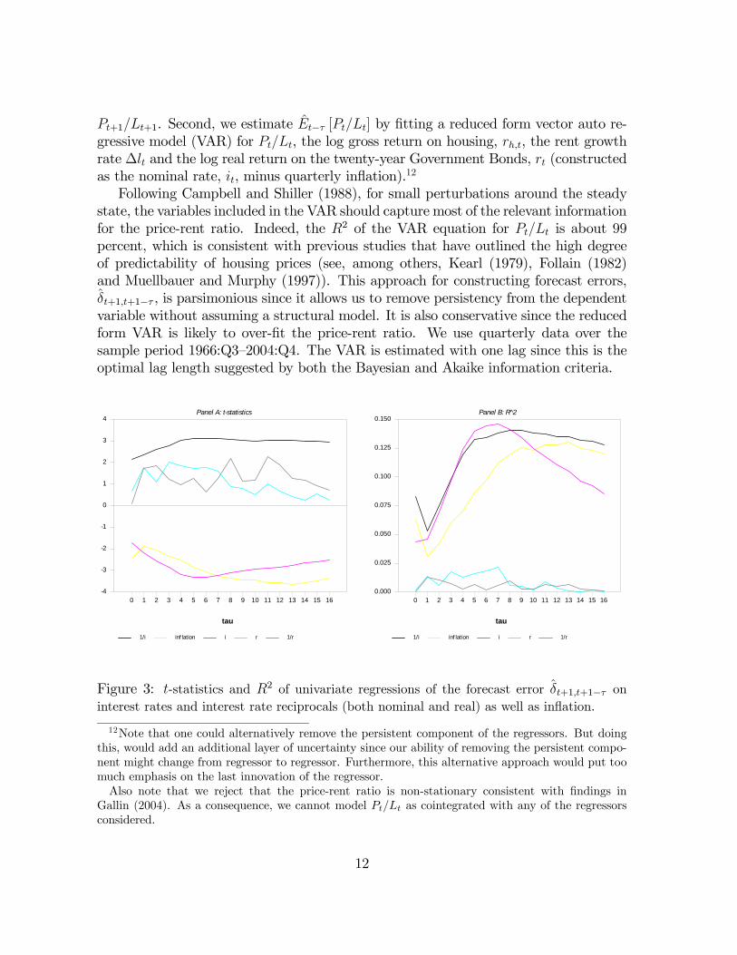
Pt+1/Lt+1. Second, we estimate Et−τ [Pt/Lt] by fitting a reduced form vector auto re-gressive model (VAR) for Pt/Lt, the log gross return on housing, rh,t, the rent growthrate ∆lt and the log real return on the twenty-year Government Bonds, rt (constructedas the nominal rate, it, minus quarterly inflation).12

Following Campbell and Shiller (1988), for small perturbations around the steadystate, the variables included in the VAR should capture most of the relevant informationfor the price-rent ratio. Indeed, the R2 of the VAR equation for Pt/Lt is about 99percent, which is consistent with previous studies that have outlined the high degreeof predictability of housing prices (see, among others, Kearl (1979), Follain (1982)and Muellbauer and Murphy (1997)). This approach for constructing forecast errors,δt+1,t+1−τ , is parsimonious since it allows us to remove persistency from the dependentvariable without assuming a structural model. It is also conservative since the reducedform VAR is likely to over-fit the price-rent ratio. We use quarterly data over thesample period 1966:Q3—2004:Q4. The VAR is estimated with one lag since this is theoptimal lag length suggested by both the Bayesian and Akaike information criteria.

1/i inf lation i r 1/r

Panel A: t-statistics

tau

0 1 2 3 4 5 6 7 8 9 10 11 12 13 14 15 16-4

-3

-2

-1

0

1

2

3

4

1/i inf lation i r 1/r

Panel B: R 2

tau

0 1 2 3 4 5 6 7 8 9 10 11 12 13 14 15 160.000

0.025

0.050

0.075

0.100

0.125

0.150

Figure 3: t-statistics and R2 of univariate regressions of the forecast error δt+1,t+1−τ oninterest rates and interest rate reciprocals (both nominal and real) as well as inflation.

12Note that one could alternatively remove the persistent component of the regressors. But doingthis, would add an additional layer of uncertainty since our ability of removing the persistent compo-nent might change from regressor to regressor. Furthermore, this alternative approach would put toomuch emphasis on the last innovation of the regressor.Also note that we reject that the price-rent ratio is non-stationary consistent with findings in

Gallin (2004). As a consequence, we cannot model Pt/Lt as cointegrated with any of the regressorsconsidered.

12

Figure 3 summarizes the results about the predictability of the price-rent ratio.The figure plots Newey and West (1987) corrected t-statistics (Panel A) and measuresof fit (Panel B) of five univariate regressions of δt+1,t+1−τ on rt, it, 1/rt, 1/it and asmoothed moving average of inflation, πt.13 (Recall that we introduced the conventionthat for τ = 0, δt+1,t+1 = Pt+1/Lt+1). That is, the first point in each of the plottedseries corresponds to the regression output of a standard forecasting regression for theprice-rent ratio.Focusing first on τ = 0 — the standard forecasting regression — it is apparent that

the real interest rate, r, has no forecasting power for the price-rent ratio with a t-statistic (Panel A) of 0.741 and a R2 (Panel B) of about 0 percent. This is consistentwith the finding of Muellbauer and Murphy (1997) that the real interest rate has noexplanatory power for movements in the real price of residential housing. The signof the slope coefficient of the nominal interest rate, i, is negative suggesting that anincrease in the nominal interest rate reduces the price-rent ratio. The regressor isstatistically significant only at the 10 percent level and explains about 5 percent ofthe variation in the price-rent ratio. The figure also shows that lagged inflation is asignificant predictor of the price-rent ratio and that the estimated slope coefficient hasa negative sign, which is consistent with the Modigliani and Cohn (1979) argumentthat inflation causes a negative mispricing in assets. This is also consistent with thefindings of Kearl (1979) and Follain (1982) that housing demand is reduced by greaterinflation. The regressor explains about 7 percent of the time variation in Pt/Lt. Fromthe predictive regression of the price-rent ratio on 1/rt — as suggested by equation (1) —we learn that this variable is not significant nor has any forecasting power for the futureprice-rent ratio, reinforcing the conjecture that housing prices do not tend to respondto changes in the real interest rate. However, the reciprocal of the nominal interestrate, 1/it, is highly statistically significant and has a positive sign implying that theprice-rent ratio tends to comove with the valuation of agents prone to money illusion.Moreover, this regressor is able to explain about 9 percent of the time variation inthe price-rent ratio. Consistently with money illusion, inflation πt shows a significantnegative correlation with housing prices.Focusing on τ > 0, we can assess whether the regressors considered have forecasting

power for the unexpected component of price-rent changes.14 It is clear from Figure 3that the real interest rate (both in terms of r and 1/r) generally has no explanatorypower for the unexpected movements in the price-rent ratio. To the contrary, thenominal interest rate, inflation and the reciprocal of the nominal interest rate arestatistically significant forecasting variables of unexpected movements in the price-rent

13Note that the measure of inflation we use is the CPI index without housing. The smoothingwindow is of sixteen quarters and we take .9 as smoothing parameter.14Recall that if the results obtained with τ = 0 are due to the persistence of regressors and regres-

sand, we would expect the statistical significance of the regressors to be substantially reduced whenconsidering τ > 0.

13

ratio, and explain a substantial share of the time series variation of this variable.For robustness we check our results using the real interest rate implied by the yields

on inflation protected ten year government bonds, instead of using nominal interest rateminus inflation, and using the implied inflation instead of our smoothed inflation. Un-fortunately, this data is available only since 1982:Q1. Consistently with the previousresults, we find that this measure of the real interest rate also has no explanatory powerfor the price rent ratio: the regressor is not statistically significant for any horizon τand its point estimate changes sign at some horizons. Moreover, using implied infla-tion instead of smoothed inflation we obtain similar patterns as in Figure 3. The onlydifference is that implied inflation is not statistically significant at two horizon levels,τ = 1 and 2; this is likely to be due to the fact that we lose 16 years of quarterly datausing implied inflation. Similarly, the real yield spread does not seem to matter. Wedefine the real yield spread as the ten year real interest rate from inflation protectedGovernment bonds minus the three month Government bills reduced by current in-flation. Moreover, estimated real interest rate variability and inflation variability aregenerally not significant predictors of the price-rent ratio, but nevertheless add (verylittle) explanatory power when considered jointly with inflation. The nominal yieldspread seems to matter, but this might be spurious since its predictive power goesaway when we control for the persistent component of the price-rent ratio. Finally, thedefault spread, defined as the difference in yield between the Great Britain CorporateBond Yield and the ten year Government bond, has predictive power.15 Nevertheless,the default spread does not substantially reduce the statistical significance of our mainnominal regressors (πt, 1/it and it).Case and Shiller (1989, 1990) find that housing price changes are predictable and

argue that this might be at odds with market efficiency. To check whether this potentialdeparture from market efficiency is connected with money illusion, we test whetherlagged inflation and the reciprocals of the nominal and real interest rates help to predictthe first difference of the price-rent ratio. We find that (i) lagged inflation and nominalinterest rates explain 6 to 10 percent of the time series variation of the changes in theprice-rent ratio, (ii) these regressors are statistically significant at levels between oneand five percent, (iii) the estimated signs are consistent with money illusion, and (iv)the real interest rate does not have any predictive power for changes in the price-rentratio.Of course, our results only show that the implicit stochastic discount factor is

related to inflation. That is, the forecastability of the price-rent ratio could also be dueto predictable changes in the required risk-premium. This would be rational, hence itdoesn’t need to be caused by money illusion. We disentangle the role of money illusionin the next subsection.15We use the corporate default spread as a proxy for the credit market condition. Ideally, one would

like to use the spread between mortgage rates and Government Bond Yields, but this is not feasibledue to data limitations.

14

3.2 Decomposing the Inflation Effect

Inflation can affect the price-rent ratio for rational reasons. In this subsection wedifferentiate the rational effects of inflation on the price-rent ratio — through expectedfuture rent growth rates and expected future returns on housing — from the effect ofinflation on the mispricing.

3.2.1 Methodology

We follow the Campbell and Shiller (1988) methodology, but allow agents to havesubjective beliefs. Letting P be the price of housing and L be the rental payment, thegross return on housing, Rh, is given by the following accounting identity:

Rh,t+1 =Pt+1 + Lt+1

Pt.

Following Campbell and Shiller (1988), we log-linearize this relation around the steadystate but, given our focus on mispricing, we allow traders to have a probability measurefor the underlying stochastic process that is different from the objective one. As aconsequence, the steady state depends on the underlying measure of the traders. Underthe assumption that the price-rent ratio is stationary, we can log-linearize the lastequation as

rh,t+1 = (1− ρ) k + ρ (pt+1 − lt+1)− (pt − lt) +∆lt+1,

where rh,t := logRh,t, pt := logPt, lt := logLt, ∆lt := lt− lt−1, ρ := 1/¡1 + exp(l − p)

¢,

l − p is the long run average rent-price ratio, and k is a constant. The log price-rentratio can be therefore rewritten (disregarding a constant term) as a linear combinationof future rent growth, future returns on housing and a terminal value

pt − lt = limT→∞

"TX

τ=1

ρτ−1 (∆lt+τ − rh,t+τ) + ρT (pt+T − lt+T )

#. (4)

Moving to excess rent growth rates, ∆let+τ = ∆lt− rt, and excess returns (risk premia)on housing, reh,t = rh,t − rt, where rt is the real return on the long-term governmentbond (with maturity of 10 or 20 years), the price-rent ratio can be expressed as

pt − lt =∞Xτ=1

ρτ−1£∆let+τ − reh,t+τ

¤+ lim

T→∞ρT (pt+T − lt+T ) . (5)

This equality also has to hold for any realization and hence, holds in expectation forany measure.

15

ψ—Mispricing Measure. Note that if agents are not fully rational, the observedprice will deviate from the true “fundamental value” and hence the realized excessreturns reh,t+τ are also distorted. Taking expectations and assuming that the transver-sality conditions hold, yields

pt − lt =∞Xτ=1

ρτ−1Et

£∆let+τ

¤−

∞Xτ=1

ρτ−1Et

£reh,t+τ

¤=

∞Xτ=1

ρτ−1Et

£∆let+τ

¤−

∞Xτ=1

ρτ−1Et

£reh,t+τ

¤where Et is the objective expectation operator conditional on the information availableat time t and Et denotes investors’ subjective (and potentially distorted) expectation.Adding and substracting

P∞τ=1 ρ

τ−1E£∆let+τ

¤from the second equation yields

pt − lt =∞Xτ=1

ρτ−1E£∆let+τ

¤−

∞Xτ=1

ρτ−1Et

£reh,t+τ

¤+

∞Xτ=1

ρτ−1³Et − Et

´ £∆let+τ

¤| {z }

=:ψt

, (6)

where we use the convention³Et −Et

´[x] := Et [x] − Et [x] and where ψt represents

the mispricing due to a distortion of beliefs about the future rent growth rate. Ifsubjective and objective expectation were to coincide, ψt would be zero. Note also

that ψt = −P∞

τ=1 ρτ−1³Et −Et

´ £reh,t+τ

¤.

So far our analysis applies to any form of belief distortion and is not specific tomoney illusion. In order to see how our definition of mispricing can capture moneyillusion, let’s consider the following example: as in Modigliani and Cohn (1979) indi-viduals fail to distinguish between nominal and real rates of returns. They mistakenlyattribute a decrease (increase) in inflation πt to a decline (increase) in real returns, rh,t— or equivalently ignore that a decrease in inflation also lowers nominal rent growthrate (∆lt + πt), i.e. Et [∆lt+τ ] = Et [∆lt+τ − πt+τ ]. Therefore, our mispricing measurereduces to

ψt = −∞Xτ=1

ρτ−1Et [πt+τ ] . (7)

That is, the mispricing and hence the price-rent ratio are increasing as expected infla-tion declines. Note that in this particular case money illusion always causes a negativemispricing error. However, if individuals have a reference level of inflation, say π, thisis not necessarily true. In this case the last equation becomes

ψt = −∞Xτ=1

ρτ−1Et [πt+τ − π] . (8)

16

Even though the level of mispricing is different with a reference level of inflation, itscorrelation with inflation is unchanged.To construct the empirical counterpart of ψt we follow Campbell (1991) and com-

pute the objective expectations of rent growth rates using a reduced form VAR. Thevariables included in the VAR are the log excess return on housing, reh,t, the log price-rent ratio, pt − lt, the excess rent growth rate, ∆let , and the exponentially smoothedmoving average of inflation, πt. The VAR is estimated using quarterly data and thechosen lag length is one (both the Bayesian and the Akaike information criteria pre-fer this lag length for the estimated model). We obtain the empirical counterpart ofP∞

τ=1 ρτ−1Et

£reh,t+τ

¤by subtracting estimated expected rent growth terms from the log

price-rent ratio.The problem is that we do not observe Et

£reh,t+τ

¤. We follow Campbell and

Vuolteenaho (2004) and assume that Et

£reh,t+τ

¤is governed by a set of risk-factors

λt. Hence, we can writeP∞

τ=1 ρτ−1Et

£reh,t+τ

¤= a + b1λt + ξt. In order to determineP∞

τ=1 ρτ−1Et

£reh,t+τ

¤−P∞

τ=1 ρτ−1Et

£reh,t+τ

¤, we run an OLS of

P∞τ=1 ρ

τ−1Et

£reh,t+τ

¤on

the risk-factors λt.∞Xτ=1

ρτ−1Et

£reh,t+τ

¤= a+ b1λt + ξt| {z }

= ∞τ=1 ρ

τ−1Et[reh,t+τ ]

+ ψt. (9)

We use different potential risk-factors. As suggested in Campbell and Vuolteenaho(2004) we use as first risk proxy the conditional volatility of an investment that is longon housing market and short on the 10 years government bonds. That is, we constructψt as the OLS residual of the following linear regression

\P∞τ=1 ρ

τ−1Et

£reh,t+τ

¤= α+

8Xτ=0

bτ ht−τ + ψt, (10)

where the first term is constructed as \P∞τ=1 ρ

τ−1Et

£reh,t+τ

¤:= (pt − lt)−

P∞τ=1 ρ

τ−1Et

£∆let+τ

¤with Et

£∆ret+τ

¤being the τ -steps ahead VAR forecasts conditional on the data observed

up to time t. The regressors ht−τ includes seven lagged GARCH-estimates of the con-ditional volatility16 and a lagged VAR forecast of the left hand side variable. The latteracts as a control in attempt to remove ξt from the residual ψt. By doing so, we takea conservative approach in order not to overestimate the mispricing. We also reportresults using only seven lagged GARCH-estimates of the conditional volatility, denotedby ψ

0t.Note that if an individual never sells her house, she is not exposed to any housing

market risk except a potential reduction in borrowing capacity. The risk comes about16The fitted model is a ARCH-GARCH(2,2) with an AR(1) component for the mean to take into

account the persistence in housing returns.

17

only whenever she has to buy or sell a house. This is for example the case when shehas to move between areas with different house price levels. Hence, an interactionbetween the probability of moving and cross-regional variability of house prices is anatural candidate for a risk factor. We therefore introduce a proxy for this source ofrisk among the risk-factors λt. This is done by adding three additional regressors inEquation (10): the cross-regional price variability across the main 14 macro regionsof the U.K., the total within country migration normalized by total population, andthe interaction between these two variables. We denote the corresponding mispricingmeasure by ψ

00t . Finally, we also experimented with the canonical Fama-French risk

factors.Some note of caution is appropriate about this decomposition. First, the measure

of mispricing ψt can depend crucially on the chosen subjective risk factor λt — which isarbitrary. Second, for the OLS construction in Equation (10) to be correct, λt shouldbe orthogonal to ψt. Third, in deriving our ψ-mispricing we also assume that irrationalinvestors understand the iterated accounting identity in equation (4).In order to determine the link between the mispricing and inflation we regress the

empirical counterpart of ψt on a set of variables meant to capture the impact of moneyillusion on the mispricing: πt, it, log (1/it).

ε—Mispricing Measure. To derive the ψ-mispricing we assumed that the transver-sality condition holds under both the objective and the subjective measure. We nowrelax this assumption and allow for explosive paths. Moreover, we avoid having tospecify exogenous risk factors, λ, to identify the implied mispricing due to explosivepaths.We define a new measure of mispricing, εt, that under the null hypothesis of ratio-

nal pricing should be zero or at least orthogonal to proxies for money illusion. Thismispricing captures the difference in expectations about future excess rent growth ratesand housing investment risk premia plus Et

£limT→∞ ρT (pt+T − lt+T )

¤:

εt :=∞Xτ=1

ρτ−1³Et −Et

´ £∆let+τ − reh,t+τ

¤+ Et

hlimT→∞

ρT (pt+T − lt+T )i. (11)

That is, εt is the difference between observed log price-rent ratio and the log price-rent ratio that would prevail if (i) all agents were computing expectations under theobjective measure and (ii) the transversality condition under the objective measureholds, i.e. Et

£limT→∞ ρT (pt+T − lt+T )

¤= 0.

The ε-mispricing can be expressed as a violation of the transversality conditionunder the objective measure

pt − lt =∞Xτ=1

ρτ−1Et

£∆let+τ − reh,t+τ

¤+Et

hlimT→∞

ρT (pt+T − lt+T )i

| {z }=εt

.

18

To see this, take subjective expectation of equation (5) and subtract the above equationfrom it. Therefore, the ε-mispricing captures bubbles which are due to potentiallyexploding paths, including the intrinsic bubbles analyzed in Froot and Obstfeld (1991).The price patterns depicted in Figure 1 make it difficult to rule out a priori explosivepaths over certain subsamples. That is, imposing the objective transversality conditionmight be too strong an assumption. Explosive path might occur if for example agentsfail to understand that all the future realizations of returns and rent growth rates mustmap into the current price-rent ratio as Equation (4) implies. Note that we assume thatall traders have the same subjective measure. If traders have heterogeneous measuresand face short-sale constraints (as for example in Harrison and Kreps (1978)), εt couldalso be affected by a speculative component.To see how the ε-mispricing relates to money illusion consider, as we did for the

ψ-mispricing, the Modigliani and Cohn (1979) benchmark. In this case we obtain thesame result as in Equation (7) and (8) with ψt replaced by εt. That is, money illusionimplies a negative correlation between the ε-mispricing and πt, it, and − log (1/it).To estimate this mispricing we decompose the observed log price-rent ratio into

three components: the implied pricing error, εt, the discounted expected future rentgrowth, and the discounted expected future returns

pt − lt =∞Xτ=1

ρτ−1Et

£∆let+τ

¤−

∞Xτ=1

ρτ−1Et

£reh,t+τ

¤+ εt, (12)

where Et denotes conditional expectations computed using the estimated VAR de-scribed above, that is, Et

£∆let+τ

¤and Et

£∆det+τ

¤are the τ -steps ahead VAR forecasts

conditional on the data observed up to time t.

3.2.2 Empirical Evidence

In this subsection we focus on the empirical links between mispricing measures andinflation. Our first-cut analysis in Section 3.1 showed that nominal terms covary withprice-rent ratio rather than real terms. But this link might be due to rational chan-nels, frictions or money illusion. There are several rational channels through whichinflation could affect housing prices. First, if inflation damages the real economy,P∞

τ=1 ρτ−1Et

£∆let+τ

¤should be negatively related with inflation. For example, this

could be the case of stagflation caused by a cost-push shock. Second,P∞

τ=1 ρτ−1Et [rh,t+τ ]

could tend to rise if inflation makes the economy riskier (or investors more risk averse),therefore driving up the required excess return on housing investment. If any of thesewere the case, the negative correlation between price-rent ratio and inflation could sim-ply be the outcome of negative real effects of inflation or of time varying risk premiaon the housing investment.Most importantly, if there were no inflation illusion, we would expect our mispricing

measures to be uncorrelated with πt, log (1/it), and it. Instead, the Modigliani and

19

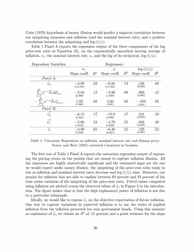
Cohn (1979) hypothesis of money illusion would predict a negative correlation betweenour mispricing measures and inflation (and the nominal interest rate), and a positivecorrelation between the mispricing and log (1/it).Table 1 Panel A reports the regression output of the three components of the log

price-rent ratio in Equation (6), on the exponentially smoothed moving average ofinflation, πt, the nominal interest rate, it, and the log of its reciprocal, log (1/it).

Dependent Variables: Regressors:πt it log (1/it)

Slope coeff. R2 Slope coeff. R2 Slope coeff. R2

Panel A:ψt −4.09

(13.479).83 −6.80

(11.765).74 .136

(8.020).69

∞Pτ=1

ρτ−1Et∆let+τ −2.58(2.390)

.12 −3.96(1.938)

.09 .093(2.083)

.12

−∞Pτ=1

ρτ−1Etreh,t+τ 1.92

(1.066).03 3.60

(.931).03 −.050

(.595).02

Panel B:

ψ0t −6.15

(2.483).17 −10.9

(2.668).17 .241

(2.823).19

ψ00t −2.60

(4.812).53 −4.79

(5.898).55 .092

(4.825).49

εt −3.90(7.946)

.65 −6.30(6.927)

.55 .129(5.991)

.52

Table 1: Univariate Regressions on inflation, nominal interest rate and illusion proxy.Newey and West (1987) corrected t-statistics in brackets.

The first row of Table 1 Panel A reports the univariate regression output of regress-ing the pricing errors on the proxies that are meant to capture inflation illusion. Allthe regressors are highly statistically significant and the estimated signs are the onewe would expect under money illusion: the mispricing of the price-rent ratio tends torise as inflation and nominal interest rates decrease and log (1/it) rises. Moreover, ourproxies for inflation bias are able to explain between 69 percent and 83 percent of thetime series variation of the mispricing of the price-rent ratio. Fitted values computedusing inflation are plotted versus the observed values of ψt in Figure 2 in the introduc-tion. The figure makes clear is that the high explanatory power of inflation is not dueto a particular subsample.Ideally, we would like to regress ψt on the objective expectation of future inflation.

One way to capture variations in expected inflation is to use the series of impliedinflation from the inflation protected ten year government bonds. Using this measureas explanator of ψt we obtain an R2 of .51 percent and a point estimate for the slope

20

coefficient of −5.06 with a t−statistics of 4.864.17The second row shows that expected future real rent growth rates seem to be nega-

tively correlated with inflation and nominal interest rate (this last variable is significantonly at the 10 percent level), and positively correlated with log (1/it). Nevertheless,only a small share (between 9 percent and 12 percent) of the time variation in expectedrent growth are explained by the regressors considered. These results are consistentwith a view in which inflation influences the rent to price ratio partially due to the factthat high inflation seems to proxy for a worsening of future economic conditions (seee.g. Fama (1981)). On the other hand, this could simply be the outcome of housingrents being more sticky than the general price level.The third row outlines that there is no significant link between inflation and (sub-

jectively expected) risk premia on the housing investment. The regressors consideredare not statistically significant and explain only between 2 percent and 4 percent of thetime series variation in expected future returns on housing. Moreover, the estimatedsigns of the regressors imply that inflation is associated with a lower risk premium onhousing investment, i.e. in times of high inflation the housing investment is consideredto be relatively less risky than investing in long-horizon government bonds. Since weuse a before-tax measure of returns on housing, this result could also be due to thefact that an increase in inflation increases the after-tax return on housing (see Poterba(1984)), therefore requiring a lower before-tax risk premium.The sum of the slope coefficients associated with each of the regressors in Table

1 Panel A is an estimate of the elasticity of the price-rent ratio with respect to thatregressor. Our results therefore imply that, on average, a one percent increase ininflation (nominal interest rate) maps into a 4.75 (7.16) percent decrease in the priceof housing relative to rent, and that the largest contribution to this negative elasticityis given by the effect of inflation (nominal interest rate) on the mispricingPanel B of Table 1 reports the regression coefficients for alternative measures of

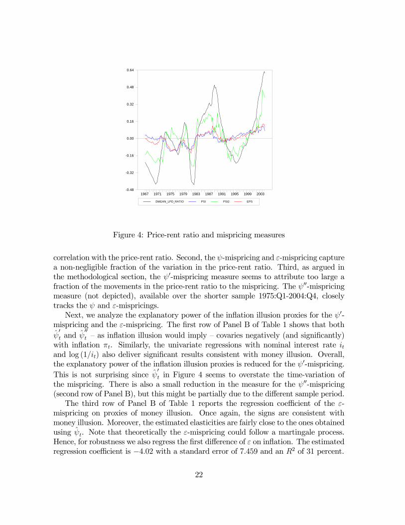
mispricings. Recall that: ψ0t is the mispricing constructed without adding controls inEquation (10)18; ψ00t is the mispricing constructed adding our “moving risk factors”;and that εt is the mispricing constructed without specifying exogenous risk factorsand measures the mispricing that maps into a violation of the transversality conditionunder the objective measure. Note that due to data limitations the ψ00t -time seriesstarts only in 1975:Q1 while the time series of the other mispricing measures run from1966:Q3—2004:Q4.The first thing of interest is to compare the sizes of the mispricing of ψ and ψ0.

Figure 4 plots the price-rent ratio, and both ψ-mispricing measures over our sampleperiod.First, notice that the measures of mispricing generally have the right pattern of

17Note that in this case, due to data availability problems, we use a sample starting in 1982:Q1.18We also tried as alternative risk factors the canonical Fama-French risk factors and obtained

similar results as for the covariance of ψ0t and the money illusing proxies.

21

DMEAN_LPD_RATIO PSI PSI2 EPS

1967 1971 1975 1979 1983 1987 1991 1995 1999 2003-0.48

-0.32

-0.16

0.00

0.16

0.32

0.48

0.64

Figure 4: Price-rent ratio and mispricing measures

correlation with the price-rent ratio. Second, the ψ-mispricing and ε-mispricing capturea non-negligible fraction of the variation in the price-rent ratio. Third, as argued inthe methodological section, the ψ0-mispricing measure seems to attribute too large afraction of the movements in the price-rent ratio to the mispricing. The ψ00-mispricingmeasure (not depicted), available over the shorter sample 1975:Q1-2004:Q4, closelytracks the ψ and ε-mispricings.Next, we analyze the explanatory power of the inflation illusion proxies for the ψ0-

mispricing and the ε-mispricing. The first row of Panel B of Table 1 shows that bothψ0t and ψ

00t — as inflation illusion would imply — covaries negatively (and significantly)

with inflation πt. Similarly, the univariate regressions with nominal interest rate itand log (1/it) also deliver significant results consistent with money illusion. Overall,the explanatory power of the inflation illusion proxies is reduced for the ψ0-mispricing.This is not surprising since ψ

0t in Figure 4 seems to overstate the time-variation of

the mispricing. There is also a small reduction in the measure for the ψ00-mispricing(second row of Panel B), but this might be partially due to the different sample period.The third row of Panel B of Table 1 reports the regression coefficient of the ε-

mispricing on proxies of money illusion. Once again, the signs are consistent withmoney illusion. Moreover, the estimated elasticities are fairly close to the ones obtainedusing ψt. Note that theoretically the ε-mispricing could follow a martingale process.Hence, for robustness we also regress the first difference of ε on inflation. The estimatedregression coefficient is −4.02 with a standard error of 7.459 and an R2 of 31 percent.

22

One worry might be that credit standards might vary over time in response tooverall economic conditions, and that this mechanism might generate the link betweenmispricing and inflation we find in the data. This is potentially important since wehave already oberved in Section 3.1 that there is a statistically significant link betweenprice-rent movements and the default spread (which is meant to capture the overalleconomic condition of the credit market). To assess the relevance of time-variationof credit market conditions, we regress our mispricing measures on inflation and thedefault spread jointly. We find that for all the measures of mispricing default spreadis not statistically significant after controlling for inflation and that the measures of fitdo not increase by more than 1 percent.Next, the mispricing might be linked to the volatitilty of inflation more than the

level itself. We check this hypothesis by running multivariate regressions of our mispric-ing measures on inflation and an estimate of conditional inflation volatility.19 We findthat the conditional volatility of inflation has no explanatory power for both mispricingmeasures after controlling for the level of inflation.Overall, the results in Table 1 suggest that money illusion can explain a large share

of the mispricing in the housing market and that the negative correlation betweeninflation and the rent-price ratio is mainly due to the effect of money illusion on themispricing. Nevertheless, our findings could be rationalized by some forms of marketfrictions. Section 4 addresses this alternative hypotheses formally.

3.2.3 Robustness Analysis

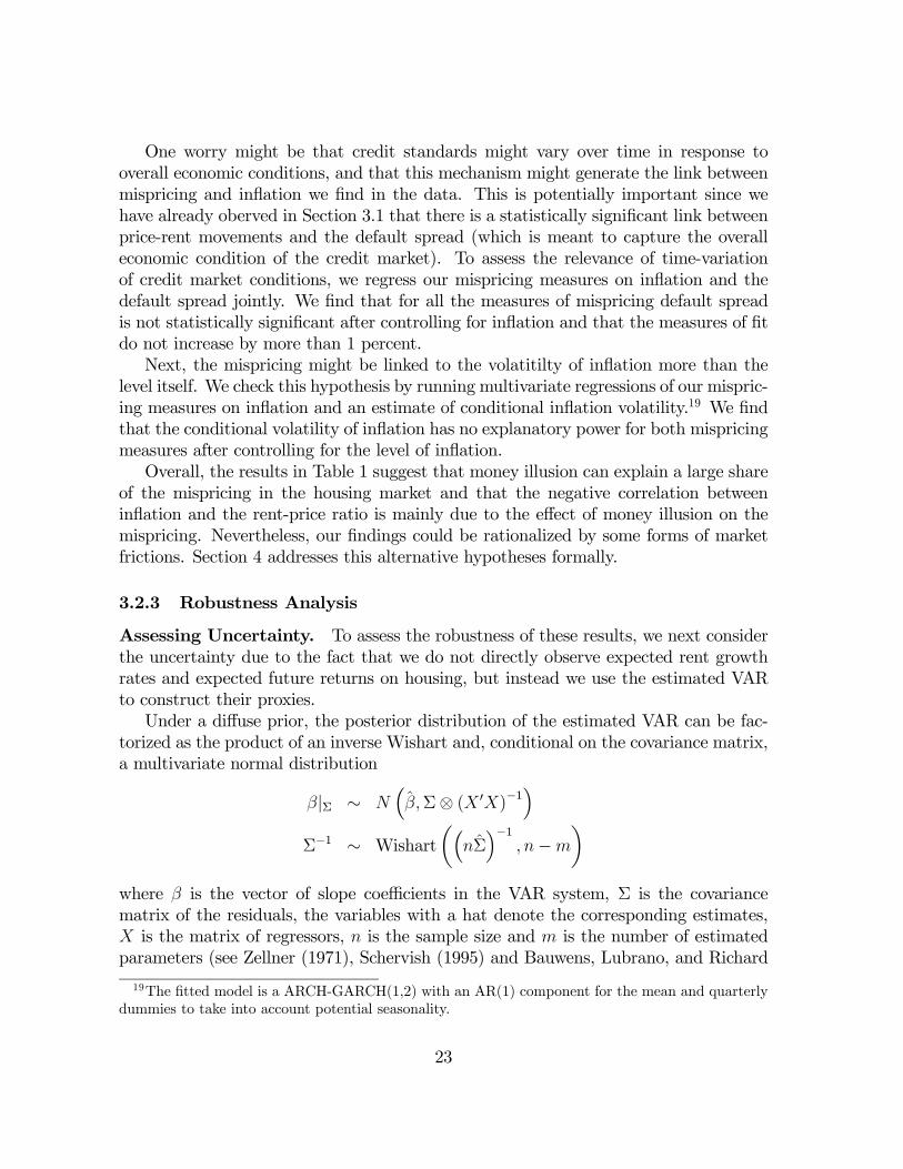
Assessing Uncertainty. To assess the robustness of these results, we next considerthe uncertainty due to the fact that we do not directly observe expected rent growthrates and expected future returns on housing, but instead we use the estimated VARto construct their proxies.Under a diffuse prior, the posterior distribution of the estimated VAR can be fac-

torized as the product of an inverse Wishart and, conditional on the covariance matrix,a multivariate normal distribution

β|Σ ∼ N³β,Σ⊗ (X 0X)

−1´

Σ−1 ∼ Wishartµ³

nΣ´−1

, n−m

¶where β is the vector of slope coefficients in the VAR system, Σ is the covariancematrix of the residuals, the variables with a hat denote the corresponding estimates,X is the matrix of regressors, n is the sample size and m is the number of estimatedparameters (see Zellner (1971), Schervish (1995) and Bauwens, Lubrano, and Richard

19The fitted model is a ARCH-GARCH(1,2) with an AR(1) component for the mean and quarterlydummies to take into account potential seasonality.

23

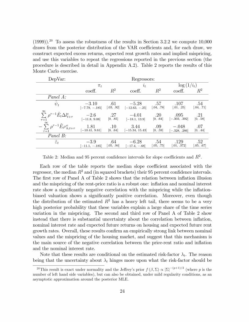
(1999)).20 To assess the robustness of the results in Section 3.2.2 we compute 10,000draws from the posterior distribution of the VAR coefficients and, for each draw, weconstruct expected excess returns, expected rent growth rates and implied mispricing,and use this variables to repeat the regressions reported in the previous section (theprocedure is described in detail in Appendix A.2). Table 2 reports the results of thisMonte Carlo exercise.

DepVar: Regressors:πt it log (1/it)

coeff. R2 coeff. R2 coeff. R2

Panel A:ψt −3.10

[−7.79, −.185].61

[.03, .92]−5.28

[−12.63, −.25].57

[.04, .78].107[.01, .25]

.54[.04, .71]

∞Pτ=1

ρτ−1Et∆let+τ −2.6[−11.8, 9.08]

.27[0, .85]

−4.01[−18.1, 13.9]

.20[0, .64]

.095[−.303, .392]

.21[0, .58]

−∞Pτ=1

ρτ−1Etreh,t+τ 1.81

[−10.41, 9.61].10[0, .64]

3.44[−15.34, 15.43]

.09[0, .59]

−.048[−.328, .286]

.07[0, .44]

Panel B:εt −3.9

[−11.1, −.185].64

[.05, .94]−6.28

[−17.4, −.68].54

[.05, .75].129

[.01, .372].52

[.05, .67]

Table 2: Median and 95 percent confidence intervals for slope coefficients and R2.

Each row of the table reports the median slope coefficient associated with theregressor, the medianR2 and (in squared brackets) their 95 percent confidence intervals.The first row of Panel A of Table 2 shows that the relation between inflation illusionand the mispricing of the rent-price ratio is a robust one: inflation and nominal interestrate show a significantly negative correlation with the mispricing while the inflation-biased valuation shows a significantly positive correlation. Moreover, even thoughthe distribution of the estimated R2 has a heavy left tail, there seems to be a veryhigh posterior probability that these variables explain a large share of the time seriesvariation in the mispricing. The second and third row of Panel A of Table 2 showinstead that there is substantial uncertainty about the correlation between inflation,nominal interest rate and expected future returns on housing and expected future rentgrowth rates. Overall, these results confirm an empirically strong link between nominalvalues and the mispricing of the housing market, and suggest that this mechanism isthe main source of the negative correlation between the price-rent ratio and inflationand the nominal interest rate.Note that these results are conditional on the estimated risk-factor λt. The reason

being that the uncertainty about λt hinges more upon what the risk-factor should be

20This result is exact under normality and the Jeffrey’s prior f (β,Σ) ∝ |Σ|−(p+1)/2 (where p is thenumber of left hand side variables), but can also be obtained, under mild regularity conditions, as anasymptotic approximation around the posterior MLE.

24

than upon how it is estimated. To address this we perform a similar robustness exerciseusing the ε-mispricing — that does not depend on exogenous risk-factors. These resultsare reported in Panel B of Table 2 and — as in Panel A — are very similar to the onesin Table 1.

Assessing the Role of the Business Cycle. Unlike the price-dividend ratio in thestock market, the observed price-rent ratio is a less precise measure since the housingprice index reflects all types of dwellings while the rent index tends to overweightsmaller and lower quality dwellings.The prices of high quality houses appreciate at a higher rate during booms, and

depreciate more during recessions, than cheaper houses do (see, among others, Poterba(1991) and Earley (1996)). This might cause the measured price-rent ratio to comovewith the business cycle. Hence, if inflation and the nominal interest rate had a clearbusiness cycle pattern, our estimated mispricing measures could show a spurious cor-relation with these variables.Figure 8 in Appendix A.3 plots the time series of the U.K. exponentially smoothed

quarterly inflation, the return on the twenty-year Government Bonds, and the Hodrickand Prescott (1997) filtered estimate of the GDP business cycle. The figure shows thatthere is no strong contemporaneous correlation of inflation and nominal interest rateswith the business cycle (the correlation coefficients are −.16 and −.15 respectively).This suggests that the high degree of explanatory power that inflation and the nominalinterest rate have for the housing market mispricing is unlikely to be due to the comove-ment of these variables with the business cycle. In Appendix A.3 we address this issueformally, and we find that the inclusion of the business cycle in the OLS regressionsfor the mispricing measures (i) does not drive out the statistical significance of πt, itand log (1/it), (ii) does not significantly change the point estimates of the elasticitiesof the mispricing reported in Table 1, (iii) does not significantly increase our ability toexplain the time variation in the mispricing, (iv) and that the business cycle alone hasvery little (in the case of ψt and εt) or no (in the case of ψ

0t) explanatory power for the

mispricing measures.

4 Market Frictions

The previous section documents a strong link between mispricings in the housing mar-ket and inflation, and suggest money illusion as the driving mechanism of this rela-tionship. However, a potential alternative explanation of this finding is the presenceof housing market frictions. In this section we formally investigate this competinghypothesis.

25

4.1 Tilt Effect

Our empirical results are consistent with money illusion. Nevertheless, we could becapturing the tilt effect of inflation which potentially generates a negative relationshipbetween inflation and housing prices. The tilt effect refers to a particular form ofliquidity constraint. It is best understood by comparing the real repayment profiles ofa mortgage with and without inflation. Suppose agents can only enter fixed nominalrepayment mortgages. The real repayment profiles of such a contract are depicted inFigure 5 for a zero and a positive inflation environment.

0 2 4 6 8 10 12 14 16 18 20 22 24 26 28 30

0.5

1.0

t years

Figure 5: Real mortgage payments over time in a zero inflation environment (dashedline) and 5 percent inflation environment (solid curve).

Without inflation the real mortgage payments are constant, while in an inflationaryenvironment the real mortgage payments decrease over time. In order to keep the realnet present value the same in the two environments, the initial payments have to behigher in a world with non-zero inflation. That is, the real repayment profile is tiltedtowards the earlier periods. In other words, when inflation is high, the financial burdenis “front-loaded” and the mortgage-payment to income ratio is higher in the early yearsof the mortgage. Hence, liquidity constraints are more likely to bind and agents are lessable to leverage. In turn, a more binding constraint in the first period of the mortgagedepresses housing demand and prices. Note that if liquidity constraint were to bebinding for a large set of agents, we would expect the price-rent, and the mispricingmeasures, to be linked to movements in the real interest rate — we have seen in previoussections that this is not the case.To test whether the tilt effect drives our results we perform two types of tests.First, note that the intercept of the repayment scheme is proportional to the nominal

interest rate, i, and that it is related to inflation only insofar as it affects the nominalinterest rate. That is, once one controls for the nominal interest rate, inflation shouldnot matter if the tilt effect is the driving force of our results. On the other hand, if themispricing is driven by money illusion, it should be related to inflation π as stressed

26

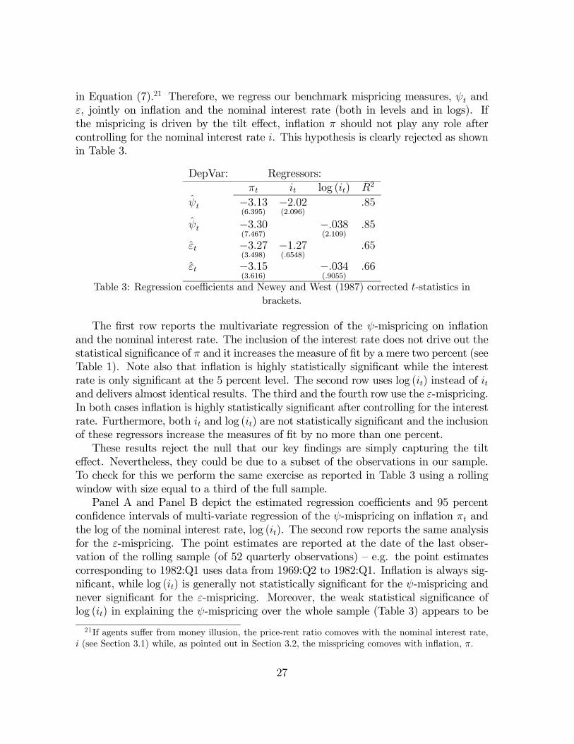
in Equation (7).21 Therefore, we regress our benchmark mispricing measures, ψt andε, jointly on inflation and the nominal interest rate (both in levels and in logs). Ifthe mispricing is driven by the tilt effect, inflation π should not play any role aftercontrolling for the nominal interest rate i. This hypothesis is clearly rejected as shownin Table 3.

DepVar: Regressors:πt it log (it) R2

ψt −3.13(6.395)

−2.02(2.096)

.85

ψt −3.30(7.467)

−.038(2.109)

.85

εt −3.27(3.498)

−1.27(.6548)

.65

εt −3.15(3.616)

−.034(.9055)

.66

Table 3: Regression coefficients and Newey and West (1987) corrected t-statistics inbrackets.

The first row reports the multivariate regression of the ψ-mispricing on inflationand the nominal interest rate. The inclusion of the interest rate does not drive out thestatistical significance of π and it increases the measure of fit by a mere two percent (seeTable 1). Note also that inflation is highly statistically significant while the interestrate is only significant at the 5 percent level. The second row uses log (it) instead of itand delivers almost identical results. The third and the fourth row use the ε-mispricing.In both cases inflation is highly statistically significant after controlling for the interestrate. Furthermore, both it and log (it) are not statistically significant and the inclusionof these regressors increase the measures of fit by no more than one percent.These results reject the null that our key findings are simply capturing the tilt

effect. Nevertheless, they could be due to a subset of the observations in our sample.To check for this we perform the same exercise as reported in Table 3 using a rollingwindow with size equal to a third of the full sample.Panel A and Panel B depict the estimated regression coefficients and 95 percent

confidence intervals of multi-variate regression of the ψ-mispricing on inflation πt andthe log of the nominal interest rate, log (it). The second row reports the same analysisfor the ε-mispricing. The point estimates are reported at the date of the last obser-vation of the rolling sample (of 52 quarterly observations) — e.g. the point estimatescorresponding to 1982:Q1 uses data from 1969:Q2 to 1982:Q1. Inflation is always sig-nificant, while log (it) is generally not statistically significant for the ψ-mispricing andnever significant for the ε-mispricing. Moreover, the weak statistical significance oflog (it) in explaining the ψ-mispricing over the whole sample (Table 3) appears to be

21If agents suffer from money illusion, the price-rent ratio comoves with the nominal interest rate,i (see Section 3.1) while, as pointed out in Section 3.2, the misspricing comoves with inflation, π.

27

Mis

pric

ing

mea

sure

s psi

eps

pi log(i)Panel A

1980 1982 1984 1986 1988 1990 1992 1994 1996 1998 2000 2002 2004-7

-6

-5

-4

-3

-2

-1

0Panel B

1980 1982 1984 1986 1988 1990 1992 1994 1996 1998 2000 2002 2004-0.20

-0.15

-0.10

-0.05

-0.00

0.05

0.10

0.15

Panel C

1980 1982 1984 1986 1988 1990 1992 1994 1996 1998 2000 2002 2004-7.5

-5.0

-2.5

0.0Panel D

1980 1982 1984 1986 1988 1990 1992 1994 1996 1998 2000 2002 2004-0.15

-0.10

-0.05

0.00

0.05

0.10

0.15

0.20

Figure 6: Multivariate regression of mispricing measures on inflation, π, and log interestrate, log (i), over rolling samples.

driven by the last 4 years of data. This last point is confirmed by an expanding windowregression exercise (not reported here). Furthermore, the same qualitative results wereobtained using the level of the nominal interest rate, it instead of log (it).Second, we now present an alternative test to discriminate between the money

illusion and the tilt-effect hypotheses based on the evolution of the mortgage marketover time. Note that in our example the tilt effect arises since the nominal mortgagepayments are constant, but more flexible mortgage contracts might reduce or eliminateit. Indeed, in the real world, agents can use multiple alternative financing schemesavailable on the market that are not affected by the tilt effect. For example this is thecase for flexible interest rate mortgages, price level adjusted mortgages (PLAM) or thegraduate payment mortgages (GPM).22 This is especially true in the United Kingdom,where PLAM and GPM were available at least since the early 1970’s. Furthermore,new, more flexible, mortgage products were introduced over the years in all major

22On the other hand, Spiegel (2001) provides a rationale for endogenous credit rationing in thehousing market due to moral hazard.

28

countries. In the U.S. for example, interest only mortgages, which substantially lowerthe initial payments, have become very popular in recent years.23 Hence, we wouldexpect that the importance of the tilt effect — if it is there — declines over time. Thatis, the negative elasticity of the mispricing to inflation should become less negative overthe sample period.We empirically assess this hypothesis. Figure 7 depicts point estimates and Newey

and West (1987) 95 percent confidence intervals of the univariate regressions of theestimated mispricing on πt, it, and 1/it over a time-varying sample. We use the firstten years of data to obtain an initial estimate of the slope coefficient associated witheach regressor, and we then add one data point at a time and update our estimates. Forexample, the point corresponding to 1992 first quarter is the estimated slope coefficientover the sample 1966 second quarter to 1992 first quarter.Figure 7 Panels A, for the ψ-mispricing, and Panel D, for the ε-mispricing, reveal

that the trend goes, if anything, in the opposite direction of what we would expect ifthe tilt effect were the driving mechanism behind the empirical link between housingprices and inflation. Over time, the negative relation between mispricing and inflationbecomes more negative. The elasticity with respect to the interest rate is essentiallyflat (Panels B and E). Only the elasticity with respect to the log of the nominal interestrate reciprocal seems to decline at the end of the sample for the ψ-mispricing (PanelC), but this reduction is not statistically significant, while it is essentially flat forthe ε-mispricing (Panel F). Overall, these findings suggest that it is unlikely that thetilt effect is the mechanism behind the empirical link between housing mispricing andinflation.How do the findings in Figure 7 square with money illusion? Money illusion does

not have a clear implication as to whether the elasticity of mispricing to inflation shouldvary over time. Nevertheless, the decline in the negative slope coefficient (in Panel Aand D) is consistent with a setting in which households attention to inflation dependson the recent history of inflation. Money illusion is very costly after and during aperiod of high inflation. Hence, households are more attentive to inflation and lessprone to money illusion. In contrast, the cost of money illusion is perceived to be lowafter and during a period of low inflation — as in the last part of our sample — andhence money illusion is more wide-spread increasing the elasticity of the mispricing toinflation.

4.2 Lock-in effect

When inflation and interest rates creep up, households that have secured a non-portablemortgage with a low fixed nominal interest rate in the past might be reluctant to buy

23See, for exampe, Lowenstein’s article in the New York Times on June 5, 2005 which cites theLehman Brothers report “The Changing Landscape of the Mortgage Market” which describes therecent increase in interest-only mortgages.

29

Mis

pric

ing

mea

sure

s psi

eps

pi i log(1/i)Panel A

1977 1981 1985 1989 1993 1997 2001-4.8

-4.4

-4.0

-3.6

-3.2

-2.8Panel B

1977 1981 1985 1989 1993 1997 2001-11

-10

-9

-8

-7

-6

-5Panel C

1977 1981 1985 1989 1993 1997 20010.075

0.100

0.125

0.150

0.175

0.200

0.225

0.250

0.275

0.300

Panel D

1977 1981 1985 1989 1993 1997 2001-5.5

-5.0

-4.5

-4.0

-3.5

-3.0

-2.5

-2.0

-1.5

-1.0Panel E

1977 1981 1985 1989 1993 1997 2001-11

-10

-9

-8

-7

-6

-5

-4

-3

-2Panel F

1977 1981 1985 1989 1993 1997 20010.04

0.08

0.12

0.16

0.20

0.24

0.28

Figure 7: Point estimates and 95 percent Newey and West (1987) corrected confidencebounds of slope coefficients as sample size increases.

30

a new, better quality house. This in turn could depress the demand for high-qualityhouses and lower the supply for low-quality houses. Therefore, given that the pools ofrental houses and houses on the market for sale are not perfectly symmetric, this couldbe the driving force of the empirical link between the price-rent ratio and the nominalinterest rate.Noticing that this “lock-in effect” is asymmetric — since it predicts an additional

reduction in housing demand for buying only when the interest rate is above the locked-in interest rate — we can perform a series of tests to assess this hypothesis.First, we run a set of regressions of our mispricing measures, ψ and ε, on the interest

rate and inflation interacted with a dummy variable that captures upward movementsin the interest rate over the last four quarters.That is we run

μt = ai + bi1dtit + bi2 (1− dt) it + eit

μt = aπ + bπ1dtπt + bπ2 (1− dt)πt + eπt

where μt is either ψt or εt, and dt is an indicator function of upward movements inthe nominal interest rate it. The lock-in effect suggests that the coefficient estimateb·1 should be different from b·2. However, we cannot reject that b·1 = b·2 for bothregressions and both mispricing measures.Second, using rolling samples (containing 10 years of observations each) we test

three separate hypotheses: Corr [R2t ,Dt] 6= 0; Corr [R2t , it] 6= 0; andCorr£R2t , pt − lt

¤6=

0, where R2t is the measure of fit of the regression of ψ on i in each rolling sample, Dt

is the average dt on a given subsample, and pt − lt is the average log price-rent ratio ina given subsample. All theses hypotheses are rejected at standard confidence levels.These results may not be surprising since most mortgages are portable in the U.K..

This is unlike in the U.S. where a large share of the mortgage contracts are not portable.Nevertheless, as in the U.K., all stated hypotheses can be rejected with U.S. data alsoexcept for Corr [R2t ,Dt] 6= 0.

5 Cross-regional Heterogeneity

In the previous section, we document money illusion as an aggregate phenomenon thatcan generate house price run ups without changes in economic fundamentals. In thissection we explore whether money illusion can be reconciled with the observed regionalheterogeneity in price behavior within a country. In order to do this we shift our focusfrom the U.K. to the U.S. housing market because the cross-sectional heterogeneity ismore prominent in the U.S. and more regional data is available. We first documentmoney illusion in the aggregate U.S. housing market. We then document heterogeneityin housing supply elasticity at the state level and explain how money illusion and

31

heterogeneity in supply elasticity can rationalize the heterogeneity in regional pricedynamics.

5.1 Aggregate U.S.-Evidence

In this section we examine the link between housing market mispricing measures andnominal values in the U.S. following the same procedure as in Section 3.2. The sampleperiod available runs from 1970:Q1—2004:Q3. Univariate regression results are reportedin Table 3. The first row shows that the proxies considered are all significant explana-tory variables for the mispricing. Moreover, the sign of the estimated elasticity is theone we would expect under inflation illusion: the mispricing of the price-rent ratiotends to rise as inflation and nominal interest rates decrease. The coefficient estimatesfor the U.S. data are similar to the ones for the U.K. The measures of fit are somewhatsmaller compared to the U.K. case, but this is likely to be due to the shorter sampleperiod and poorer quality of U.S. data. An exception is the R2 for the expected rentgrowth rate, which is higher for the U.S.For a review of the measurement problems in U.S. data on housing see McCarthy

and Peach (2004). Nevertheless, the R2 ranges from 28 percent when the explana-tory variable is the nominal interest rate to 45 percent when we use inflation as theexplanatory variable of the mispricing.

Dependent Variables: Regressors:πt it log (1/it)

coeff. R2 coeff. R2 coeff. R2

Panel A:ψt −6.65

(4.525).45 −6.30

(3.182).28 .141

(4.256).35

∞Pτ=1

ρτ−1Et∆let+τ −2.87(6.572)

.65 −3.46(6.170)

.65 .066(4.693)

.60

−∞Pτ=1

ρτ−1Etreh,t+τ .76

(.211).01 4.65

(1.130).05 −.066

(.734).03

Panel B:εt −10.2

(5.148).48 −6.86

(2.648).15 .159

(3.238).21

Table 4: Univariate Regressions on inflation, nominal interest rate and illusion proxy.Newey and West (1987) corrected t-statistics in brackets.

The second row shows that there is a significantly negative (positive) correlationbetween inflation and nominal interest rate (log of the nominal interest rate reciprocal)and expected future rent excess growth rates. This could either be a consequenceof a negative effect of inflation on the real economy or due to a higher degree ofstickiness in housing rents than in the general price level. The regressors considered

32

are able to explain between 60 to 65 percent of the time series variation in expectedfuture growth rates. The last row shows that there is a no statistically significant linkbetween inflation/nominal interest rate and future risk premia on housing investment.The coefficients for the U.S. are slightly lower compared to the U.K. coefficient, whichis consistent with the different tax treatment of mortgage interest payments in bothcountries. Overall, these results imply a negative elasticity of the price-rent ratio toinflation (nominal interest rates) of about 8.7 (5.1) and that the largest contributionto this comes from the effect of inflation (nominal interest rate) on mispricing.Table 5 reports the results of a Monte Carlo exercise (described in Section A.2 of the

Appendix) analogous to the one presented in Section 3.2, which, as in the case of U.K.data, confirms the soundness of the empirical link between mispricing in the housingmarket and inflation, nominal interest rate and the log of the nominal interest ratereciprocal. On the other hand, it shows that there is substantial uncertainty about therational links between inflation (nominal interest rate) and the price-rent ratio, eventhough both variables show a significantly negative correlation with the risk premiumon the housing investment.

DepVar: Regressors:πt it log (1/it)

coeff. R2 coeff. R2 coeff. R2

Panel A:ψt −6.06

[−7.32, −2.76].44

[.06, .66]−5.84

[−7.12, −2.14].27

[.03, .66].130

[.070, .155].35

[.06, .60]∞Pτ=1

ρτ−1Et∆let+τ −2.86[−8.17, 1.53]

.59[.01, .96]

−3.45[−7.27, −0.53]

.52[.02, .71]

.066[.003, .149]

.51[.01, .70]

−∞Pτ=1

ρτ−1t Ereh,t+τ .44[−4.84, 3.21]

.01[0, .09]

4.23[1.12, 5.82]

.04[.01, .12]

−.023[−.097, 0]

.07[0, .15]

Panel B:εt −10.2

[−16.2, −7.25].48

[.36, .62]−6.83

[−10, −4.79].15

[.11, .21].159

[.115, .25].21

[.16, .26]

Table 5: Median and 95 percent confidence intervals for slope coefficients and R2. U.S. data.

5.2 The U.S. Regional Housing Markets

In the previous section we documented the presence of money illusion in the aggregateU.S. housing market. Yet house price shifts often vary significantly across differentregions of the same country. In the U.S., the recent price increase seems to be muchless pronounced in the Midwest compared to the coastal regions. In this section weinvestigate whether money illusion can be reconciled with these heterogeneous pricedynamics.

33

First, it should be mentioned that this regional heterogeneity is less extreme thanit appears at first sight, once one separates property prices into land value and build-ing value. Davis and Palumbo (2006) analyze 46 large metropolitan areas in the U.S.and find that the appreciation of residential land since the mid-1980s is a widespreadphenomenon because the price of residential land has risen much faster than housingconstruction costs. The different rates of increase in land and building value couldpartially explain the observed cross-sectional heterogeneity in property price move-ments. To be more explicit, consider the following stylized example. Suppose in thelow population density Midwest, 80 percent of the property value reflects the value ofthe building, while in New York City the building value is say only 10 percent of theproperty value. Then the same percentage increase in land price would cause a muchlarger increase in property value in New York than in the Midwest.Second, it is often argued that regional heterogeneity of property values is due to

different housing supply elasticities. This could be another reason why money illusionimpacts house prices across various regions differently. To understand how supplyelasticity interacts with money illusion, let us consider a simple setting in which housingdemand, D (P, π), is decreasing in housing price, D1 := ∂D/∂P < 0, and inflation,D2 := ∂D/∂π < 0, due to money illusion. The supply of housing S (P,X) is increasingin house prices, S1 := ∂S/∂P > 0, and also affected by cost shifters X. Applying theimplicit function theorem on the market clearing condition to obtain dP/dπ and takingthe derivative with respect to the slope of the supply function S1, one obtains

d (dP/dπ)

dS1= − D2

(D1 − S1)2 > 0. (13)

Since S1 is inversely proportional to the elasticity of supply, this last equation showsthat money illusion can generate large price movements in area characterized by alow elasticity of supply (high S1).24 Therefore, we study whether S1 changes acrossregional markets.25 To do this, we nest our work in the housing supply literatureand try to estimate the elasticity of new housing starts to house price changes. Theexisting literature has produced a wide range of both point estimates and conflictingmethodologies (see DiPasquale (1999) for a survey). Previous literature has focusedon the empirical link between new housing starts and the housing price level. On theother hand Mayer and Somerville (1996) argue that housing starts are a flow variableand therefore should be a function of other flow variables, and focus therefore on thelink between housing starts and housing price changes. Also, using a panel of U.S.quarterly state-level data over the period 1975:Q1—2005:Q4, we find that the OFHEOhousing price indices seem to contain a unit root (as in Gallin (2003, 2004)), while

24If builders also suffer from money illusion, this result still holds as long as households suffer frommoney illusion more than builders.25In Glaeser, Gyourko, and Saks (2007) heterogeneity in supply elasticity is the endogenous outcome

of households voting on zoning regulations.

34

this hypothesis can be rejected for the new housing starts series. As a consequence, weregress housing starts in state i, Iit, on the one-year price changes ∆Pit.Note that our main interest is not to estimate the supply elasticity itself but to

assess how it varies across different regions. In particular, we explore whether therelative degree of land availability generates heterogeneity in supply elasticity. For thispurpose, we focus on an interaction term between prices, ∆Pit, and population density,pdit. The previous literature has shown population density to be relevant in explainingcross-sectional housing price differences since it captures the relative scarcity of land(see e.g. Voith (1996)).Regressing new housing starts on price change, we would expect a positive coef-

ficient for an upward-sloping supply curve. But, if high population density reducesthe elasticity of supply, adding as a regressor price changes interacted with populationdensity, ∆Pit × pdit, we would expect a negative coefficient.In order to distinguish movements along the supply curve from movements of the

supply curve, we introduce as controls a set of construction-cost shifters. The additionalregressors are the one-year change in the real ENR building cost index, the real interestrate on the 3-months T-bill as a proxy for the cost of capital, and the one-year changein the per capita state-specific real wage as a proxy for labor cost changes.In our panel regressions we also control for state fixed effects and state specific

cyclicality using state specific quarterly dummies. In addition, we add to our regressionsa third order polynomial in a linear time trend and the time series of state populationdensities. We also add lagged new housing starts, Iit−1, to capture the high degree ofpersistence of the regressand. Population density is constructed removing water areafrom the total state area and the series is normalized to have unit mean. Nominalvalues are made real using the CPI less shelter. Unfortunately, we do not have data onland prices at the state level to add as an additional control. Following the previousliterature, we include inflation to the regressions, and we also interact inflation withpopulation density.Since we have quarterly data over the period 1975:Q1—2005:Q4 for 50 states plus the

District of Columbia, our sample size of 5865 observations implies that our regressionshave more than 5640 degrees of freedom. Since prices, construction costs and wages arepotentially endogenously determined, we need to perform IV estimates. As instrumentswe use all the exogenous variables and their first lag, all the dummies and trends, andthe first two lags of the endogenous variables. Weak instruments do not seem to be anissue since the measures of fit of the first stage regression range between .70 for pricechanges to .82 for the ENR building cost index. We also employ a heteroskedasticityand autocorrelation consistent estimator of the covariance matrix with Newey andWest(1987) windows of 12 lags, and corrected to take into account the use of instrumentalvariables.

35

Regressors: R2

Iit−1 ∆Pit ∆Pit × pdit πt πt × pdit rt(1) .901

(47.24).843(1.871)

−.064(2.796)

−10.9(4.424)

.172(.0311)

.97

(2) .901(47.54)

.710(1.659)

−11.26(4.471)

.274(3.152)

.195(.0354)

.97

(3) .901(47.17)

.833(1.844)

−.064(2.787)

−11.14(2.515)

.228(2.758)

.140(.0253)

.97

Table 6: Regressions of housing starts on its lag, yearly price-change, inflation and oninteraction terms. Coefficients of additional controls are not reported. Corrected t-statistics

in brackets.

Table 6 reports the point estimates of the main coefficients of interest in our panelregression. The first row shows, as expected, a positive correlation between pricechanges and new housing starts but the regression coefficient is significant only at the10 percent level. Most importantly, the interaction term between price changes andpopulation density is negative and highly statistically significant, suggesting that theelasticity of housing supply is reduced in areas where land is relatively scarce. Inflationshows a significantly negative relationship with housing starts as already found in Topeland Rosen (1988). This last finding is consistent with the proxy effect of inflation butalso with a setting in which rational builders are aware that households suffer frommoney illusion. Indeed, Topel and Rosen (1988) find the effect of inflation on housingstarts to be too strong to be explained by their rational investment model. The realinterest rate is not significant. The second row replaces the interaction term∆Pit×pditwith the interaction of inflation and population density, πt×pdit. The point estimate ofthe other coefficients is almost unchanged and price changes are statistically significantonly at the 10 percent level while inflation is highly significant and the real interestrate is not. Interestingly, πt×pdit has a positive sign suggesting that inflation tends toreduce supply less in high density areas. The last row uses both interaction terms, andconfirms the results of the previous regressions and also shows that the two interactionterms have different information content since they are both strongly significant evenwhen employed jointly.For robustness, we also performed regressions in which we modeled parametrically

autoregression in the residuals, without obtaining significantly different results. Fi-nally, we performed structural estimations of the investment model of Topel and Rosen(1988), but adding an interaction term between prices, inflation and population den-sity. Even though these last estimations regress housing starts on price levels, insteadof price changes, we obtained qualitatively similar results.Overall, the results in this section reconcile the presence of money illusion as an

aggregate phenomenon and regional differences in price behavior.

36

6 Conclusion

This paper studies the link between inflation and housing prices. Our first-cut approachshows that the housing price-rent ratio is not affected by the real, but by the nominalinterest rate. Moreover, we decompose time-series movements of the price-rent rationinto movements in a rational component and an implied mispricing component. Wefind that movements in inflation explain a large share of the time variation of themispricing. These results are robust and hold for both the U.K. and the U.S. housingmarkets.Two potential explanations of the link between the price-rent ratio and inflation

naturally arise. First, inflation might make the economy riskier, or agents more riskaverse, therefore increasing risk premia and driving down real estate prices. Second,current high inflation might be disruptive for the economy and/or inflation might proxyfor future downturns, therefore depressing current housing value. We do not findsupportive evidence for the first hypothesis while the evidence in favor of the secondhypothesis does not seem to be robust in the housing market context.We also investigate possible explanations due to market frictions. First, inflation

may tilt real mortgage payments towards the earlier years, making funding constraintspotentially more binding. Second, an increase in inflation may dampen the demand forhousing upgrades from individuals that have locked-in low nominal interest rates on anexisting mortgages. Our extensive series of tests suggests that these market frictionsare unlikely to be the mechanism behind the link between inflation and housing marketmispricing. We also document substantial heterogeneity in housing supply elasticityacross U.S. states due to differences in relative land scarcity, and we argue that thiscould reconcile our evidence of an aggregate money illusion phenomenon in housingmarkets with the observed heterogeneity in regional price behavior.We therefore interpret our findings as supportive evidence for the money illusion

hypothesis. Our findings provide a new argument in favor of price stability, sinceresidential housing is the single largest asset class of households.Several potential future research avenues come to mind. First, the analysis could

be extended to a cross-section of countries to assess the role of institutional features.Preliminary results for Australia are also supportive of the money illusion hypothesis.Second, it would be interesting to study the common root of money illusion in marketsas different as the residential housing market, the commercial real estate market andthe stock and bond markets.

References

Abreu, D., and M. K. Brunnermeier (2003): “Bubbles and Crashes,” Economet-rica, 71(1), 173—204.

37

Amihud, Y. (1996): “Unexpected Inflation and Stock Returns Revisited - Evidencefrom Israel,” Journal of Money, Credit, and Banking, 28(1), 22—33.

Asness, C. S. (2000): “Stocks versus Bonds: Explaining the Equity Risk Premium,”Financial Analysts Journal, 56(2), 96—113.

(2003): “Fight the Fed Model,” Journal of Portfolio Management, 30(1),11—24.

Ayuso, J., and F. Restoy (2003): “House Prices and Rents: An Equilibrium AssetPricing Approach,” working paper, Bank of Spain.

Basak, S., and H. Yan (2005): “Equilibrium Asset Prices and Investor Behavior inthe Presence of Money Illusion,” working paper, London Business School.

Bauwens, L., M. Lubrano, and J.-F. Richard (1999): Bayesian Inference inDynamic Econometric Models. Oxofrd University Press, Oxford.

Bernanke, B., and M. Gertler (1989): “Agency Costs, Net Worth, and BusinessFluctuations,” American Economic Review, 79(1), 14—31.

Bernanke, B., M. Gertler, and S. Gilchrist (1996): “The Financial Acceleratorand the Flight to Quality,” Review of Economics and Statistics, 48, 1—15.

Blinder, A. (2000): “Comment on “Near-Rational Wage and Price Setting and theLong-Run Phillips Curve”,” Brookings Papers on Economic Activity, 2000(1), 50—55.

Boudoukh, J., and M. Richardson (1993): “Stock Returns and Inflation: A Long-Horizon Perspective,” American Economic Review, 83(5), 1346—1355.

Campbell, J. Y. (1991): “A Variance Decomposition for Stock Returns,” EconomicJournal, 101, 157—79.

Campbell, J. Y., and R. J. Shiller (1988): “The Dividend-Price Ratio and Ex-pectations of Future Dividends and Discount Factors,” Review of Financial Studies,1(3), 195—228.

Campbell, J. Y., and T. Vuolteenaho (2004): “Inflation Illusion and StockPrices,” American Economic Review Papers and Proceedings, 94, 19—23.

Case, K. E., and R. J. Shiller (1989): “The Efficiency of the Market for Single-Family Homes,” American Economic Review, 79, 125—137.

(1990): “Forecasting Prices and Excess Returns in the Housing Market,”AREUEA Journal, 18, 253—273.

38

Clayton, J. (1996): “Rational Expectations, Market Fundamentals and HousingPrice Volatility,” Real Estate Economics, 24(4), 441—470.

Cohen, R. B., C. Polk, and T. Vuolteenaho (2005): “Money Illusion in theStock Market: The Modigliani-Cohn Hypothesis,” Quarterly Journal of Economics,120(2), 639—668.

Davis, M. A., and M. G. Palumbo (2006): “The Price of Residential Land in LargeU.S. Cities,” mimeo, Federal Reserve Board.

DeLong, J. B., A. Shleifer, L. H. Summers, and R. J. Waldmann (1990):“Noise Trader Risk in Financial Markets,” Journal of Political Economy, 98(4),703—738.

DiPasquale, D. (1999): “Why Don’t We Know More about Housing Supply?,” Jour-nal of Real Estate Finance and Economics, 18, 9—23.

Earley, F. (1996): “Leap-Frogging in the UK Housing Market,” Housing Finance,32, 7—15.

Fama, E. F. (1981): “Stock Returns, Real Activity, Inflation and Money,” AmericanEconomic Review, 71(4), 545—565.

Fama, E. F., and G. W. Schwert (1977): “Asset Returns and Inflation,” Journalof Financial Economics, 5(2), 115—146.

Fehr, E., and J.-R. Tyran (2001): “Does Money Illusion Matter?,” American Eco-nomic Review, 91(5), 1239—1262.

Ferson, W. E., S. Sarkissian, and T. Simin (2002): “Spurious Regressions inFinancial Economics?,” NBER Working Paper 9143.

Fisher, I. (1928): Money Illusion. Adelphi, New York.

(1930): The Theory of Interest. Maxmillan, New York.

Follain, J. (1982): “Does Inflation Affect Real Behaviour? The Case of Housing,”Southern Economic Journal, 48, 570—582.

Froot, K. A., and M. Obstfeld (1991): “Intrinsic Bubbles: The Case of StockPrices,” American Economic Review, 81(5), 1189—1214.

Gallin, J. (2003): “The Long-Run Relationship between House Prices and Income:Evidence from Local Housing Markets,” Board of Governors of the Federal ReserveDiscussion Paper 2003-17.

39

(2004): “The Long-Run Relationship between House Prices and Rents,” Boardof Governors of the Federal Reserve Discussion Paper 2004-50.

Genesove, D., and C. Mayer (2001): “Loss Aversion and Seller Behavior: Evidencefrom the Housing Market,” Quarterly Journal of Economics, 116(4), 1233—1260.

Glaeser, E. L., J. Gyourko, and R. E. Saks (2007): “Why Have Housing PricesGone Up?,” American Economic Review Papers and Proceedings (forthcoming).

Gultekin, N. B. (1983): “Stock Market Returns and Inflation: Evidence from OtherCountries,” Journal of Finance, 38(1), 49—65.

Harrison, J. M., and D. Kreps (1978): “Speculative Investor Behavior in a StockMarket with Heterogeneous Expectations,” Quarterly Journal of Economics, 89,323—336.

Hendry, D. F. (1984): “Econometric Modelling of House Prices in the United King-dom,” in Econometrics and Quantitative Economics, ed. by D. F. Hendry, and K. F.Wallis. Basil Balckwell, Oxford.

Himmelberg, C., C. Mayer, and T. Sinai (2005): “Assessing High House Prices:Bubbles, Fundamentals, and Misperceptions,” Journal of Economic Perspectives,forthcoming.

Hodrick, R. J., and E. C. Prescott (1997): “Postwar U.S. Business Cycles: AnEmpirical Investigation,” Journal of Money, Credit, and Banking, 29(1), 1—16.

Kearl, J. (1979): “Inflation, Mortgage, and Housing,” Journal of Political Economy,85(5), 1115—1138.

Kiyotaki, N., and J. Moore (1997): “Credit Cycles,” Journal of Political Economy,105(2), 211—248.

Leontief, W. (1936): “The Fundamental Assumptions of Mr. Keynes’ MonetaryTheory of Unemployment,” Quarterly Journal of Economics, 5(4), 192—197.

Lessard, D., and F. Modigliani (1975): “Inflation and the Housing Market: Prob-lems and Potential Solutions,” Sloan Management Review, pp. 19—35.

Lintner, J. (1975): “Inflation and Security Returns,” Journal of Finance, 30(2),259—280.

Mankiw, G., and D. Weil (1989): “The Baby Boom, the Baby Bust, and theHousing Market,” Regional Science and Urban Economics, 19(2), 235—258.

40

Mayer, C. J., and C. T. Somerville (1996): “Regional Housing Supply and CreditConstraints,” New England Economic Review, pp. 39—51.

McCarthy, J., and R. W. Peach (2004): “Are Home Prices the Next ‘Bubble’?,”FRBNY Economic Policy Review, 10(3), 1—17.

Modigliani, F., and R. Cohn (1979): “Inflation, Rational Valuation and the Mar-ket,” Financial Analysts Journal, 37(3), 24—44.

Muellbauer, J., and A. Murphy (1997): “Booms and Busts in the UK HousingMarket,” The Economic Journal, 107, 1701—1727.

Newey, W. K., and K. D. West (1987): “A Simple, Positive Semidefinite, Het-eroskedasticity and Autocorrelation Consistent Covariance Matrix,” Econometrica,55, 703—708.

Patinkin, D. (1965): Money, Interest, and Prices. Harper and Row, New York.

Piazzesi, M., and M. Schneider (2006): “Inflation Illusion, Credit and AssetPrices,” mimeo.

Poterba, J. M. (1984): “Tax Subsidies to Owner-Occupied Housing: An Asset-Market Approach,” Quarterly Journal of Economics, 99(4), 729—752.

(1991): “House Price Dynamics: The Role of Tax Policy and Demography,”Brookings Papers on Economic Activity, 1991(2), 143—203.

Ritter, J. R., and R. S. Warr (2002): “The Decline of Inflation and the Bull Marketof 1982-1999,” Journal of Financial and Quantitative Analysis, 37(1), 29—61.

Scheinkman, J., and W. Xiong (2003): “Overconfidence and Speculative Bubbles,”Journal of Political Economy, 111(6), 1183—1219.

Schervish, M. J. (1995): Theory of Statistics. Springer, New York.

Shafir, E., P. Diamond, and A. Tversky (1997): “Money Illusion,” QuarterlyJournal of Economics, 112(2), 341—374.

Sharpe, S. A. (2002): “Reexamining Stock Valuation and Inflation: The Implicationsof Analysts’ Earning Forecasts,” Review of Economics and Statistics, 84(4), 632—648.

Shiller, R. J. (1997a): “Public Resistance to Indexation: A Puzzle,” BrookingsPapers on Economic Activity, 1997(1), 159—228.

(1997b): “Why Do People Dislike Inflation?,” in Reducing Inflation: Motiva-tion and Strategy, ed. by C. Romer, and D. H. Romer. University of Chicago Press,Chicago.

41

(2005): Irrational Exuberance. Princeton University Press, Princeton andOxford, 2nd edn.

Spiegel, M. (2001): “Housing Return and Construction Cycles,” Real Estate Eco-nomics, 29(4), 521—551.

Stein, J. C. (1995): “Prices and Trading Volume in the Housing Market: A Modelwith Downpayment Effects,” Quarterly Journal of Economics, 110(2), 379—406.

Thaler, R. (1980): “Toward a Positive Theory of Consumer Choice,” Journal ofEconomic Behavior and Organization, 1.

Tobin, J. (1972): “Inflation and Unemployment,” American Economic Review, 62(1),1—18.

Topel, R., and S. Rosen (1988): “Housing Investment in the United States,” Journalof Political Economy, 96(4), 718—740.

Torous, W., R. Valkanov, and S. Yan (2005): “On Predicting Stock Returns withNearly Integrated Explanatory Variables,” Journal of Business, 78(1), forthcoming.

Tsatsaronis, K., and H. Zhu (2004): “What Drives Housing Price Dynamics:Corss-country Evidence,” BIS Quarterly Review, pp. 65—78.

Tucker, D. P. (1975): “The Variable-Rate Graduated-Payment Mortgage,” RealEstate Review, pp. 71—80.

Tversky, A., and D. Kahneman (1981): “The Framing of Decisions and the Psy-chology of Choice,” Science, 211, 453—458.

Voith, R. (1996): “The Suburban Housing Market: The Effects of City and SuburbanJob Growth,” Federal Reserve Bank of Philadelphia Business Review, pp. 1—13.

Wheaton, W. C. (1985): “Life-Cycle Theory, Inflation, and the Demand for Hous-ing,” Journal of Urban Economics, 18, 161—179.

Zellner, A. (1971): An Introduction to Bayesian Inference in Econometrics. Wiley,New York.

42

A Appendix

A.1 Data Description

A.1.1 U.K. Data

The housing price series is from the Nationwide Building Society, and covers the sampleperiod 1966:Q2—2005:Q1. Over the period 1966:Q2—2005:Q5 the index is constructedas a weighted average using floor area, therefore allowing to control for the influenceof house size. Over the periods 1974:Q1—1982:Q4, and 1983:Q1—1992:Q1 additionalcontrols (for region, property type, etc.) have been added in the construction of theindex. Since 1993 the index also takes into account changes in the neighborhoodclassification. The rent series is constructed combining several sources available throughthe Office of National Statistics. Over the period 1966:01—1987:01 we use the CTMKLA:HRA series of rents on dwellings paid by tenants in the U.K. and we combineit with the data on the stock of housing available trough the Office of the DeputyPrime Minister. Over the period 1987:02—1987:12 we use the RPI-SGPE rent series ofmonthly percent changes over one month. Over the period 1988:01—2005:02 we use theCZCQ - RPI series of percent changes in rent over one year. The rent-free tenancies areexcluded from the calculation of average rents. To obtain a series in levels for the price-rent ratio we scale the index series to match the level of the average price-rent ratio in1990. As interest rate we use the 20-year par yield on British Government Securitiesavailable over the sample 1963:Q4—2004:Q4. All the results presented in the paperare based on the longest possible sample given the data at hand (1966:Q2—2004:Q4).The cross-regional price variability is computed as the variance of the Nationwidequarterly log price index across the main 14 macro regions of the U.K. available overthe period 1973:Q3—2005:Q4. Total within country migration probability is computedover the period 1975:Q1—2004:Q4 from the NHSCR quarterly tables using total inflowsand outflows of England, Wales, Scotland and Northern Ireland normalized total U.K.resident population.The implied inflation series, available over the period 1982:Q1—2005:Q1, is from the

Bank of England and is constructed using the inflation protected 10 years governmentsecurities.The real GDP measure is the seasonally adjusted, chained volume measures with

constant 2002 prices and is available over the period 1955:Q1—2005:Q1 from the Officeof National Statistics.

A.1.2 U.S. Data

Aggregate Data. To construct the housing price index series we use (i) the weightedrepeat-sale housing price index form the Office of Federal Housing Enterprise Oversightover the sub-sample 1976:01—2004:03 and the (ii) Census Bureau housing price index

43

(obtained through the Bank of International Settlements) over the period 1970:01—1975:04. To construct the rent index we use the CPI-Rent from the Bureau of LaborStatistics. We re-scale the indexes to levels to match the historical average of the U.S.price-rent ratio over the same sample (as reported in Ayuso and Restoy (2003)). Aslong-run interest rate we use the return on the 10-year Treasury bill. As measure ofinflation we use the CPI index without housing.

Regional Data. As housing price index we use the quarterly OFHEO Housing PriceIndex (HPI) for 50 states and the District of Columbia over the period 1975:Q1—2005:Q4. The availability of these data series determines the sample of the panelanalysis. As new housing starts measure we use the quarterly not seasonally adjustedstate level Private Housing Units Permits Authorized series from the Markets databaseavailable through Global Insight. The labor cost measure is the state level quarterlytotal Wages and Salary series provided by the Bureau of Economic Analysis. As statepopulation measure we use the yearly total resident population estimates provided bythe Bureau of Census of the U.S. Department of Commerce. The series are interpolatedat quarterly frequency. We compute state land area as total area minus water areafrom the Census 2000 data. As building cost proxy we use the aggregate quarterlynot seasonally adjusted Engineering News Record (ENR) Building Cost Index (BCI)average of 20 U.S. cities. The BCI is a weighted index of skilled labor, structural steelshapes, portland cement and lumber costs. Nominal values are made real using theCPI less shelter price index.

A.2 Assessing Uncertainty

To assess uncertainty in the regression results in Table 2, we report 95 percent confi-dence intervals for the estimated slope coefficients and R2constructed via Monte Carlointegration by drawing form the posterior distribution of the estimated VAR coeffi-cients. We proceed as follows:

1. We draw covariance matrices Σ from the inverseWishart with parameters³nΣ´−1

and n−m.

2. Conditional on Σ we draw a vector of coefficients for the VAR, β, from

β ∼ N³β, Σ⊗ (X 0X)

−1´.

3. Using the draws of the VAR slope coefficients, β, we construct expected dis-counted sums of rent excess growth rates (

P∞τ=1 ρ

τ−1Et∆let+τ) and obtain theexcess housing returns (

P∞τ=1 ρ

τ−1Etreh,t+τ) in order to compute pricing errors ψ

and ε.

44

4. We then regress ψt, ε,P∞

τ=1 ρτ−1Et∆let+τ and

P∞τ=1 ρ

τ−1t Etr

eh,t+τ on πt, it and

the log of the inflation-biased evaluation 1/it, and we store the estimated slopecoefficients and measures of fit.

5. We repeat this procedure 10,000 times and compute confidence intervals for theOLS slope coefficients associated with πt, it and the log of 1/it, and for thecorresponding measures of fit, from the corresponding percentiles of the MonteCarlo iterations.

A.3 Assessing the Role of the Business Cycle

To construct a business cycle proxy for the U.K. we follow Hodrick and Prescott (1997),that is we estimated the following state-space model

∆yt = gt + ct (14)

gt = 2gt−1 − gt−2 + vt

where ∆yt is GDP growth from quarter t − 5 to quarter t, gt is the unobserved statevariable meant to capture the smooth time varying trend, and ct is the cyclical compo-nent. The variance of vt is normalized to be 1/1600 times the variance of the cyclicalcomponent, ct, as it is customary with quarterly data. This state-space representationis estimated via Kalman filter and Kalman smoother.Figure 8 plots the time series of the U.K. exponentially smoothed quarterly infla-

tion, the return on the twenty-year Government Bonds, and the Hodrick and Prescott(1997) filtered estimate of the GDP business cycle. The HP-estimate seems to capturefairly well the business cycle over the period considered. Moreover, there is no clearcomovment between inflation and the business cycle.Table A1 reports OLS regressions of our mispricing measures (εt and ψt) on the

variables meant to capture money illusion (πt, it and log (1/i)) and the business cyclecomponent of GDP identified by the H-P filter (ct).

45

INF_SMOOTH B_CYCLE INT

1966 1970 1974 1978 1982 1986 1990 1994 1998 2002-0.06

-0.04

-0.02

0.00

0.02

0.04

0.06

0.08

Figure 8: U.K. business cycle and inflation

Regressors:Row: Dep. variable: ct πt it log (1/i) R2

(1) ψt 0.81(1.959)

.07

(2) 0.32(2.135)

−4.00(13.761)

.85

(3) 0.378(2.168)

−6.64(11.137)

.76

(4) 0.50(2.590)

0.13(8.121)

.71

(5) ψ0t 1.11

(0.963).01

(6) 0.36(0.349)

−5.98(2.279)

.17

(7) 0.41(0.369)

−10.5(2.436)

.17

(8) 0.55(0.503)

0.24(2.605)

.19

(9) εt 0.85(2.201)

.07

(10) 0.41(2.281)

−3.80(7.801)

.67

(11) 0.49(2.158)

−6.10(6.399)

.57

(12) 0.60(2.462)

0.12(5.769)

.5646

Table A1. Regressions on business cycle fluctuations, inflation, nominal interest rate, andillusion proxy. Newey and West (1987) corrected t-statistics in brackets.

It is clear from the first and fifth rows of Table A1 that the business cycle as little(in the case of εt) or no (in the case of ψt) explanatory power for the mispricing.The remaining rows clearly show that the inclusion of the business cycle in the OLSregressions for the mispricing a) does not drive out the statistical significance of πt,it and log (1/it), b) does not significantly change the point estimates of the elasticitiesof the mispricing reported in Table 1, c) does not increase significantly our ability toexplain the time variation in the mispricing (comparing Table A1 to Table 1, we havethat the increase in R2 is ranges from 0 to 4 percent, and there is virtually no increasesin the — non reported — R2).

47