WP/05/144

Money Demand and Inflation in Dollarized Economies:

The Case of Russia

Nienke Oomes and Franziska Ohnsorge

© 2005 International Monetary Fund WP/05/144

IMF Working Paper

European Department

Money Demand and Inflation in Dollarized Economies: The Case of Russia

Prepared by Nienke Oomes and Franziska Ohnsorge1

Authorized for distribution by Lorenzo Figliuoli

July 2005

Abstract

This Working Paper should not be reported as representing the views of the IMF. The views expressed in this Working Paper are those of the author(s) and do not necessarily represent those of the IMF or IMF policy. Working Papers describe research in progress by the author(s) and are published to elicit comments and to further debate.

Money demand in dollarized economies often appears to be highly unstable, making it difficult to forecast and control inflation. In this paper, we show that a stable money demand function for Russia can be found for “effective broad money,” which includes an estimate of foreign cash holdings. Moreover, we find that an excess supply of effective broad money is inflationary, while other excess money measures are not, and that effective broad money growth has the strongest and most persistent effect on short-run inflation. JEL Classification Numbers: E31, E41, F31 Keywords: money demand, inflation, dollarization, currency substitution, Russia Author(s) E-Mail Address: noomes@imf.org, fohnsorge@imf.org

1 For useful comments and suggestions, the authors are indebted to Olena Bilan, Goohoon Kwon, Bogdan Lissovolik, David Owen, Antonio Spilimbergo, Poul Thomsen, Anna Vdovichenko, two anonymous referees, and seminar participants at the IMF, the Central Bank of Russia, the European Central Bank, the New Economic School in Moscow, and the UACES conference on “Monetary Policy in Selected CIS Countries.” Special thanks to Sergey Nikolaenko of the Bureau of Economic Analysis in Moscow for sharing his data and expertise on estimating foreign currency holdings in Russia. The authors are responsible for any remaining errors. A shorter version of this paper is forthcoming in the Journal of Comparative Economics.

- 2 -

Contents Page

I. Introduction......................................................................................................................... 3

II. Russia’s Inflation Experience During the Past Decade ...................................................... 6

III. Analytical Framework ........................................................................................................ 8 A. Long-Run Inflation .................................................................................................. 9 B. Long-Run Money Demand..................................................................................... 12 C. Short-Run Inflation Dynamics ............................................................................... 16

IV. Conclusion ........................................................................................................................ 19 Appendix I. Estimating Foreign Currency in Circulation in Russia ..................................................... 22 II. The Contribution of Valuation Effects to Effective Broad Money Growth ..................... 24 III. Unit Root and Cointegration Tests ................................................................................... 26 References............................................................................................................................... 28 Figures 1. Core and Headline CPI and Ruble Broad Money................................................................. 3 2. Effective Broad Money Components.................................................................................... 3 3. Monetary Aggregates and Exchange Rate............................................................................ 4 4. Headline CPI and Ruble-Dollar Exchange Rate ................................................................... 7 5. Headline CPI and Monetary Aggregates .............................................................................. 7 Appendix Figures A1. Estimates of Foreign Cash Holdings in Russia................................................................ 23 A2. Inflation and Contributions to Effective Broad Money Growth ...................................... 24 Tables 1. Selected Transition Economies: Money Growth and Inflation, 2003................................... 6 2. Estimated Long-Run Cointegration Equation for Inflation, April 1996–January 2004 ..... 11 3. Estimated Long-Run Money Demand Equations, April 1996–January 2004 .................... 15 4. Estimated Short-Run Inflation Equations, January 1997–January 2004 ............................ 18 Appendix Tables A1. Unit Root Tests for Regression Variables, 1996:4–2004:1 ............................................. 26 A2. Cointegration Tests for Long-Run Inflation and Money Demand, 1996:4–2004:1 ........ 27

- 3 -

I. INTRODUCTION

The relationship between money growth and inflation in Russia has recently seemed difficult to understand. In 2003, ruble broad money growth accelerated from 35 to 50 percent, while headline inflation fell markedly, from 15 to 12 percent. Since 2004, the opposite phenomenon has occurred: ruble broad money growth slowed substantially, from almost 60 percent to around 25 percent by mid-2005, while inflation has picked up (Figure 1). A substantial part of the movements in headline inflation were due to temporary or seasonal factors, as indicated by the fact that core inflation was roughly stable.2 Nevertheless, the stability of core inflation is difficult to reconcile with these sharp movements in money growth.

In this paper, we argue that taking into account foreign cash holdings is crucial for understanding the relationship between money growth and inflation in Russia. Since the early 1990s, foreign currency, mainly the U.S. dollar, has generally served all standard money functions in Russia.3 It is important, therefore, to include foreign cash holdings outside the banking system in the definition of money. While data on foreign cash holdings are unavailable for most countries, such data are available for Russia, and are described in Appendix I. Although the exact amount of foreign cash holdings is subject to considerable uncertainty, it is clear that, following a period of rapid dollarization (i.e., an increase in the share of foreign cash and foreign currency deposits) until end-1999, Russia

2 Core inflation in Russia excludes the prices of seasonal fruits and vegetables, fuel, public transportation, postal services, telecommunication, and housing and communal services. The prices of many of these goods and services are administered by the government.

3 That is, foreign currency has been used in Russia as a unit of account, a store of value, and a means of payment. While foreign currency is not legal tender in Russia, the U.S. dollar and, increasingly, the euro have been de facto accepted means of payment, in particular for large purchases such as real estate and cars.

Figure 1. Core and Headline CPI and Ruble Broad Money(12-month percent change)

9

11

13

15

17

19

21

23

25

Jun-01 Dec-01 Jun-02 Dec-02 Jun-03 Dec-03 Jun-04 Dec-04 Jun-050

10

20

30

40

50

60

70

80

Headline inflation (left scale)

Core inflation(left scale)

Ruble broad money growth(right scale)

Figure 2. Effective Broad Money Components(In percent)

0%

20%

40%

60%

80%

100%

1992

1993

1994

1995

1996

1997

1998

1999

2000

2001

2002

2003

2004

2005

Forex cash Forex deposits Ruble cash Ruble deposits

- 4 -

has experienced the opposite phenomenon—that is, dedollarization—in recent years.4 In particular, Figure 2 suggests that the share of foreign cash holdings in overall money demand has declined substantially, and has largely been offset by an increase in the share of ruble deposits and, to a lesser extent, ruble cash. The dynamics of dollarization appear to be related closely to movements in the exchange rate. As Figure 3 shows, the growth in ruble broad money (defined as ruble currency plus deposits, or M2) slowed during periods of ruble depreciation (e.g., during 2001 and 2002), and accelerated during periods of ruble appreciation (e.g., during 2003). A likely explanation for this strong correlation is that ruble depreciation increases the returns on holding foreign currency and, therefore, gives incentives to dollarize, while ruble appreciation increases the returns on holding ruble currency and, therefore, gives incentives to dedollarize. To the extent that dollarization and dedollarization represent mere portfolio shifts, it is perhaps not surprising that the growth in effective broad money (defined as M2 plus foreign currency deposits plus foreign cash holdings) has been much more stable than ruble broad money growth.

Previous studies of money demand in Russia, which did not include an estimate of foreign cash holdings, have found it difficult to find a stable money demand function. Banerji (2002) estimates a demand function for ruble broad money in Russia for the period June 1995–March 2001 and finds that VAR tests for the presence of a single cointegrating vector, which is one measure of money demand stability, “did not yield sensible or robust results.”5 Choudhry (1998) estimates money demand in Russia for the earlier hyperinflation period January 1992–September 1994 and also fails to find evidence for a stationary long-run relationship between real ruble money balances (ruble broad money and ruble currency) and

4 Additional evidence of dedollarization is given by balance of payments data from the Central Bank of Russia (CBR), according to which the stock of foreign cash holdings outside the banking system was roughly constant at around $35 billion from 1998 through early 2003, but has fallen by around $10 billion since then (from $36.9 billion in the first quarter of 2003 to $27.1 billion in the first quarter of 2005, with a temporary pickup in the third quarter of 2004, possibly reflecting the mini-banking crisis in July of that year).

5 Banerji (2002), footnote 6.

Figure 3. Monetary Aggregates (12-month percent change), and Exchange Rate (Ruble per U.S. Dollar)

0

10

20

30

40

50

60

70

2000 2001 2002 2003 2004 2005

25

26

27

28

29

30

31

32

33

Exchange rate (right scale)

Effective broad money growth (left scale)

Ruble broad money growth (left scale)

- 5 -

inflation.6 Bahmani-Oskooee and Barry (2000) obtain a stationary relationship for the period January 1991–June 1997, but, nevertheless, find evidence for instability of real ruble broad money demand in Russia. Studying a similar period, January 1992–July 1998, Nikolić (2000) finds that the relationship between broad money and inflation is “unstable and sensitive to changes taking place in the new economic and institutional environment” (p. 131).

In this paper, we show that including foreign cash holdings in the definition of money improves the stability of the money demand function. For the period April 1996–January 2004, we find that monetary aggregates that exclude foreign cash holdings are significantly negatively dependent on the nominal bilateral U.S. dollar depreciation rate, confirming that the U.S. dollar has been an important substitute for ruble broad money. It is perhaps not surprising, therefore, that the demand for effective broad money, which includes foreign cash holdings, does not significantly depend on depreciation, because it is unaffected by currency substitution. Additional indications that the effective broad money demand function is the most stable are that it exhibits the smallest standard errors, constant parameter estimates, and the strongest evidence for uniqueness of its cointegrating vector.

The construction of a broader, more stable, monetary aggregate can help us to better understand, and possibly predict, inflation. Using a standard approach for estimating a “long-run” inflation equation, we find that, over our sample period, nominal effective depreciation accounts for roughly 50 percent, the growth in unit labor costs for 40 percent, and utility price growth for 10 percent of inflation. Deviations from this long-run relationship can be quite persistent—they can take up to 12 months to be corrected. In addition, the short-run dynamics of inflation seem to depend importantly on effective broad money. One indication of this is that an excess supply of effective broad money does appear to be inflationary, while the excess supplies of narrower monetary aggregates do not. A second indication is that changes in effective broad money growth have the strongest and most persistent effect on short-run inflation.

Our results should be interpreted with some caution, since they depend crucially on the accuracy of the data and the appropriateness of the econometric approach. First, our estimate of foreign currency in circulation is subject to considerable uncertainty (Appendix I). Second, the strength of the short-term impact of effective broad money on inflation may be overestimated because of valuation effects (Appendix II). Third, our “long-run” cointegration results should be treated cautiously because of the relatively short time series and our ensuing choice to use monthly data and dummies for the August 1998 crisis, which may not have been sufficient to entirely remove the structural break in our series. Finally, while our methodology follows that of several other studies in the literature, the robustness of our

6 Choudhry (1998), however, does find evidence for a stationary relationship between real money balances, the inflation rate, and the rate of nominal ruble/U.S. dollar depreciation, which he interprets as evidence of currency substitution.

- 6 -

approach needs to be tested in further research using other data sources, additional variables, and different econometric specifications.

The results of this study may be relevant for other dollarized transition economies. As Table 1 shows, a number of transition economies, mostly member countries of the Commonwealth of Independent States (CIS), experienced rapid money growth in 2003 while inflation remained relatively low. In addition, several recent studies on inflation in transition economies have found a weak link between inflation and the growth of monetary aggregates that exclude foreign cash holdings.7 It may, therefore, be useful to study whether the inclusion of an estimate of foreign cash holdings can help improve the stability of money demand functions for these transition economies as well.

Inflation M21 Broad Money2

Azerbaijan 2.2 28.0 30.0Belarus 28.4 71.1 56.8Bulgaria 2.3 20.3 16.8Kazakhstan 6.4 55.1 29.2Kyrgyz Republic 2.7 33.5 33.4Russia 13.7 51.6 39.7Ukraine 5.2 43.5 47.2Source: IMF, International Financial Statistic database.1 Defined as currency outside banks, demand deposits, and time and savings deposits. 2 Defined as M2 plus foreign currency deposits at deposit money banks.

Table 1. Selected Transition Economies: Money Growth and Inflation, 2003(Average annual percent growth)

II. RUSSIA’S INFLATION EXPERIENCE DURING THE PAST DECADE

Following a period of rapid ruble depreciation and hyperinflation in the early 1990s, tight monetary and fiscal policies implemented in 1995 helped to bring down 12-month inflation from over 200 percent at end-1994 to about 20 percent at end-1996. Disinflation efforts were supported by a favorable external environment. However, short-term capital inflows and official debt relief exerted upward pressure on the exchange rate. By attempting to stem ruble 7 For Ukraine, Lissovolik (2003) finds no evidence for a significant long-run relationship between money and inflation between February 1996 and September 2002. For the Slovak Republic, Kuijs (2002) finds no direct impact of excess broad money on short-run inflation during the period March 1993–December 2000. For Georgia, Maliszewski (2003) finds that the effect of exchange rates on inflation is somewhat higher than that of money aggregates for the period January 1996 to February 2003.

- 7 -

appreciation with unsterilized foreign exchange interventions, the CBR slowed the disinflation process somewhat. To discourage speculation for ruble appreciation, an exchange rate band was introduced from July 1995, which helped stabilize exchange rate and inflation expectations further (Figure 4).

Inflation increased dramatically again following the August 1998 financial crisis. The seeds for the crisis had been sown by weak fiscal and external fundamentals, combined with contagion effects from the Asian crisis.8 In August 1998, the authorities announced a unilateral moratorium on debt payments and widened the trading band of the ruble, implying a de facto devaluation. In September 1998, the exchange rate depreciated by more than 100 percent, the immediate effect of which was a surge in monthly inflation from 3.7 percent in August to 38 percent in September 1998, and an increase in 12-month inflation from 5.6 percent in July 1998 to 126 percent by July 1999. The effect of depreciation to inflation was particularly strong given that many prices had been indexed in dollars.

Since 1999, the authorities have pursued a relatively unambitious disinflation path. A favorable external environment, in particular a recovery of oil and metals prices and ensuing current account surpluses, as well as resumed capital inflows from 2001, allowed the CBR to accumulate reserves. Since 2000, the CBR has been fighting pressures for ruble appreciation through largely unsterilized foreign exchange purchases. As a result, monetary aggregates have been growing rapidly, and further disinflation is proving difficult.

Effective broad money has grown broadly in line with inflation and exchange rate developments. As Figure 5 shows, effective broad money growth accelerated sharply during (and partly anticipating) the 1998 crisis,9 and decelerated again as inflation came down. While this is mostly a reflection 8 For more discussion on the causes of the 1998 crisis, which is beyond the scope of this paper, see, e.g., Buchs (1999), Desai (2000), and Kharas, Pinto, and Ulatov (2001).

9 The drop in all monetary aggregates in mid-1998 partly reflects a collapse of the payment system in the immediate aftermath of the crisis.

Figure 4. Headline CPI and Ruble-Dollar Exchange Rate(12-month percent change)

-50

0

50

100

150

200

250

300

350

1995 1996 1997 1998 1999 2000 2001 2002 2003 2004

CPI Inflation

Depreciation

Figure 5. Headine CPI and Monetary Aggregates(12-month percent change)

-20

0

20

40

60

80

100

120

140

160

1996 1997 1998 1999 2000 2001 2002 2003 2004

Ruble broad money growth

Effective broad money growth

CPI Inflation

- 8 -

of the revaluation of dollar-denominated assets during ruble depreciations and appreciations, more detailed calculations in Appendix II show that it also reflects a volume effect. Moreover, as we argue in Appendix II, the fact that changes in the exchange rate affect effective broad money may make it a more useful measure for explaining, and possibly predicting, inflation.

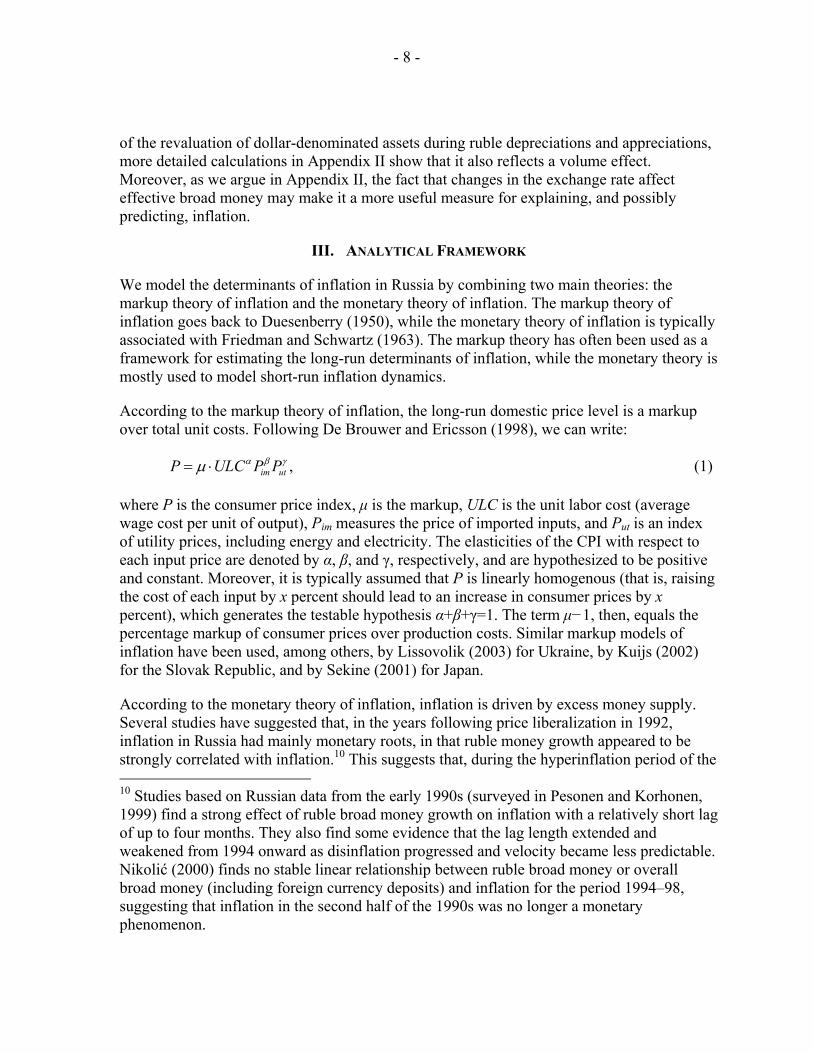
III. ANALYTICAL FRAMEWORK

We model the determinants of inflation in Russia by combining two main theories: the markup theory of inflation and the monetary theory of inflation. The markup theory of inflation goes back to Duesenberry (1950), while the monetary theory of inflation is typically associated with Friedman and Schwartz (1963). The markup theory has often been used as a framework for estimating the long-run determinants of inflation, while the monetary theory is mostly used to model short-run inflation dynamics.

According to the markup theory of inflation, the long-run domestic price level is a markup over total unit costs. Following De Brouwer and Ericsson (1998), we can write:

,im utP ULC P Pα β γµ= ⋅ (1)

where P is the consumer price index, µ is the markup, ULC is the unit labor cost (average wage cost per unit of output), Pim measures the price of imported inputs, and Put is an index of utility prices, including energy and electricity. The elasticities of the CPI with respect to each input price are denoted by α, β, and γ, respectively, and are hypothesized to be positive and constant. Moreover, it is typically assumed that P is linearly homogenous (that is, raising the cost of each input by x percent should lead to an increase in consumer prices by x percent), which generates the testable hypothesis α+β+γ=1. The term µ−1, then, equals the percentage markup of consumer prices over production costs. Similar markup models of inflation have been used, among others, by Lissovolik (2003) for Ukraine, by Kuijs (2002) for the Slovak Republic, and by Sekine (2001) for Japan.

According to the monetary theory of inflation, inflation is driven by excess money supply. Several studies have suggested that, in the years following price liberalization in 1992, inflation in Russia had mainly monetary roots, in that ruble money growth appeared to be strongly correlated with inflation.10 This suggests that, during the hyperinflation period of the 10 Studies based on Russian data from the early 1990s (surveyed in Pesonen and Korhonen, 1999) find a strong effect of ruble broad money growth on inflation with a relatively short lag of up to four months. They also find some evidence that the lag length extended and weakened from 1994 onward as disinflation progressed and velocity became less predictable. Nikolić (2000) finds no stable linear relationship between ruble broad money or overall broad money (including foreign currency deposits) and inflation for the period 1994–98, suggesting that inflation in the second half of the 1990s was no longer a monetary phenomenon.

- 9 -

early 1990s, money demand growth was negligible compared with money supply growth. In principle, however, inflationary pressures are naturally expected to arise only when money supply exceeds money demand.

We employ a two-stage estimation method that allows us to take into account both theories of inflation. In the first stage, we estimate a long-run markup equation for inflation without taking into account excess money supply (since excess money should equal zero in the long run) and we separately estimate a long-run equation for money demand, using the Johansen cointegration approach in both cases. In the second stage, we then combine the two long-run relationships in one equation that takes into account deviations from the long-run equations (i.e., the equilibrium correction terms), so as to determine the short-run dynamics of inflation.11

A. Long-Run Inflation

To estimate a long-run inflation equation for Russia, we calculate unit labor costs using industrial wage, employment, and output data, we measure import price growth by nominal effective exchange rate depreciation, and we estimate the growth in utility costs by the growth of the “paid services” component of the CPI.12 Unit labor cost are calculated as the industrial wage bill (i.e., industrial wages times industrial employment) divided by real industrial output.13 The nominal effective exchange rate is a trade-weighted average of exchange rates, and, therefore, is a better proxy for import prices than bilateral exchange rates.14 The “paid services” component of the CPI includes public transportation, housing, 11 Such a two-stage approach is commonly used for developing countries with time series data that are of limited length and that tend to be subject to significant measurement errors (e.g., Kuijs, 2002; Sacerdoti and Xiao, 2001; Williams and Adedeji, 2004). While it would obviously be preferable to estimate the two long-run equations simultaneously from one VAR, this tends to be very difficult with short time series data of limited quality that are subject to structural breaks. The advantage of separately estimating two VARs, each of which has a unique cointegrating vector, is that it is easier to find estimates close to theoretical priors. Kuijs (2002, p. 9) argues that this economic advantage outweighs the technical drawback of having a (statistically) less efficient procedure.

12 A similar variable is used in the long-run inflation equations estimated by Kuijs (2002) for the Slovak Republic, and by Lissovolik (2003) for Ukraine.

13 Since monthly industrial employment data for Russia are only available from January 1998, we used overall employment growth as a proxy for industrial employment growth for the earlier period.

14 We do not multiply the nominal effective exchange rate by foreign price levels because, during the sample period, inflation in the trading partner countries (most importantly, the EU) was low and stable compared to Russian inflation.

- 10 -

telephone subscription, electricity, water, sewage, and gas—i.e., most of the items that are also excluded from core inflation.15 An alternative, and possibly preferable, approach would be to use core inflation as the dependent variable, but this option was not available to us since Russian data on core inflation are only available from January 1999.

We can write the long-run equation for inflation as a loglinear function of unit labor costs, depreciation, and utility prices:

ln( ) ,utp ulc neer pµ α β γ= + ⋅ + ⋅ + ⋅ (2)

where p denotes the logarithm of the CPI index, neer denotes the logarithm of the nominal effective exchange rate index, ulc the logarithm of the unit labor cost index, and put the logarithm of the price index for paid services (utilities). In order to test for cointegration between these variables, it is necessary for all variables to be I(1), i.e., nonstationary in levels but stationary in differences. However, standard unit root tests, reported in Appendix III, cannot reject (at the 1 percent level) the hypothesis that all variables are nonstationary in differences, not even when we use 12-month differences to reduce seasonal effects.16 However, monthly changes in the year-on-year growth rates are found to be stationary. Although unit root tests have weak power in short time series, we consider these results sufficiently reliable to estimate the following cointegration vector:

,utp ulc neer pα β γ∆ = ⋅∆ + ⋅∆ + ⋅∆ (3)

where the ∆ signs refer to 12-month differences. That is, we assume that inflation depends for α percent on unit labor cost growth, for β percent on the nominal effective depreciation rate, and for γ percent on utility price inflation.

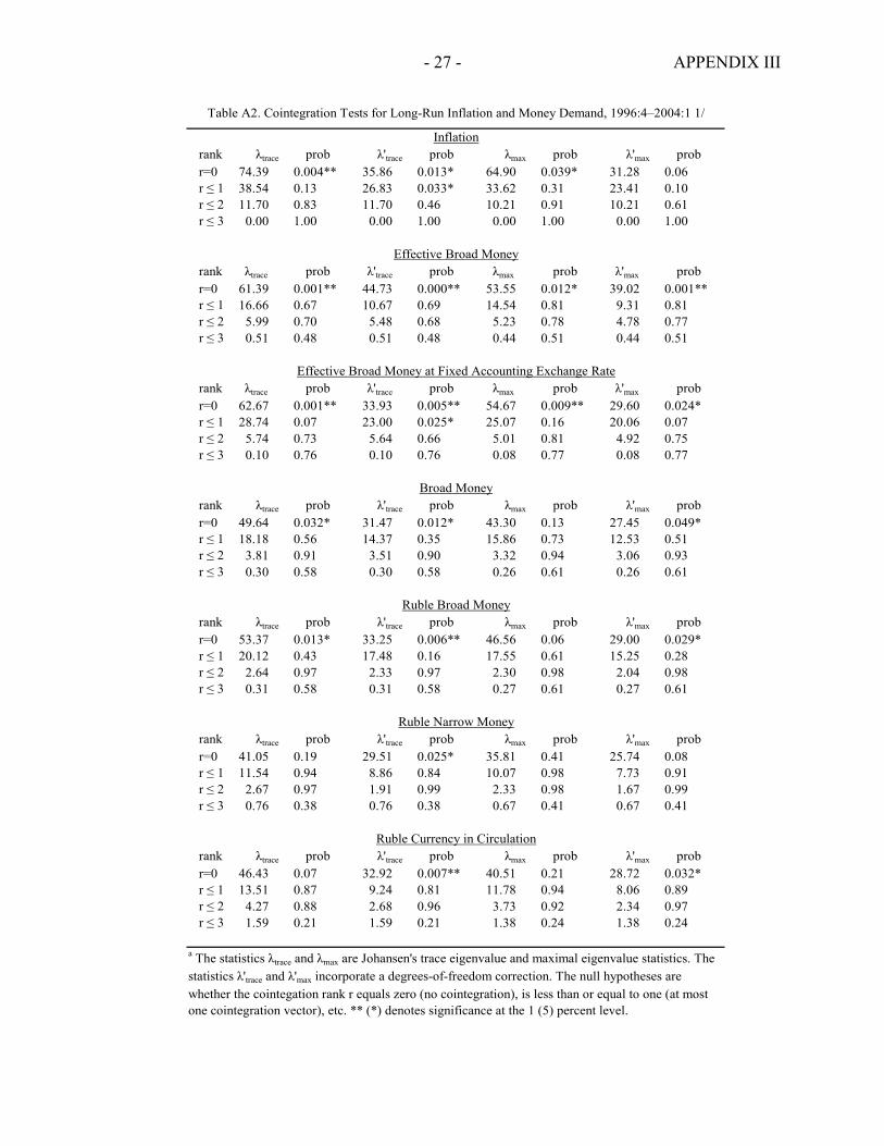
Johansen cointegration tests generally confirm the hypothesis of a unique cointegrating vector for the period April 1996–January 2004. As Table A2 in Appendix III shows, the null 15 These data are taken from Goskomstat, the state statistical committee, which publishes time series on only three subcomponents of the CPI: foodstuffs, non-food goods, and paid services. Note that, if the CPI weight of paid services was constant over time, it would be perfectly collinear with the CPI, but since the weight is time-varying, we do not consider this a problem.

16 It is possible that our failure to reject the null hypothesis that inflation is nonstationary is due to the low power of Dickey-Fuller unit root tests for relatively small samples with structural breaks. However, it is not unusual for inflation to be nonstationary. For example, the inflation rate is often included as an opportunity cost in cointegrating vectors for money demand, which is a valid procedure only if inflation is I(1). Evidence of nonstationary inflation is also reported by Celasun and Goswami (2002) for Iran, and by Budina, Maliszewski, De Menil, and Turlea (forthcoming) for Romania.

- 11 -

hypothesis of no cointegration (r = 0) is strongly rejected, while the null hypothesis that there is at most one cointegration test (r ≤ 1) cannot be rejected by three out of four cointegration tests (and for the fourth test only at the 5 percent level). Note that these tests include a small sample adjustment, which is important given the weak power of cointegration test in short time series.

The estimated cointegration relationship, normalized for inflation, suggests that long-run inflation depends for roughly 50 percent on nominal effective depreciation, for roughly 40 percent on unit labor cost growth, and for roughly 10 percent on increases in utility prices (Table 2). The estimate of the pass-through effect from nominal effective depreciation is relatively precise and robust, and close to the 0.5–0.6 pass-through estimate found by Stavrev (2003) for the nominal ruble-U.S. dollar depreciation rate.17 Without imposing the restriction that the coefficients should add up to unity, the coefficient on utility price growth is larger, and the coefficient on ULC is smaller. However, when we reestimate the equation imposing the linear homogeneity hypothesis (α+β+γ=1), a formal likelihood-ratio test shows that this hypothesis cannot be rejected at the 5 percent level. We, therefore, take the restricted long-run inflation equation to be the more economically meaningful one, although one should keep in mind that the coefficient on utility price growth is a residual.

Sum of Coefficients

Unrestricted Coefficient 0.253 ** 0.477 ** 0.457 ** 1.187Standard error 0.097 0.019 0.140

Restricted Coefficient 0.397 ** 0.494 ** 0.109 2 1.000Standard error 0.103 0.020 ...

LR test of restriction: χ2(1) =3.0548 [0.0805]

Note: ** denotes significance at the 1 percent level.1 The regression includes three lags, a constant, a trend, and four dummies: for the disinflation period in early 1996, the 1998 crisis, the August 1999 recovery from the exchange rate overshooting in August 98, and October 2000 (for 4/96 to 7/96, 8/98 to 9/98, 8/99, 10/00).2 The coefficient on utility price growth is a residual.

Table 2. Estimated Long-Run Cointegration Equation for Inflation, April 1996–January 20041

Utility Price Growth

Unit Labor Cost Growth

Nominal Effective Depreciation

17 Reestimating the equation with the bilateral rate instead of the nominal effective rate gives a very similar estimate, most likely because the nominal effective exchange rate for Russia puts a large weight on the bilateral U.S. dollar rate.

- 12 -

The estimated coefficients of the (restricted) long-run inflation equation are robust and stable over time. All coefficients, and in particular the coefficient on nominal effective depreciation, appear broadly robust to the choice of lag length (using two instead of three lags), the measure of unit labor cost (using industrial wage growth gives similar results) and the measure of import price growth (using the bilateral depreciation rate against the U.S. dollar gives similar results as using nominal effective depreciation). Moreover, the coefficient estimates remain stable even when the equation is recursively estimated, i.e., when we sequentially add new monthly observations, starting from January 2000.18

B. Long-Run Money Demand

We estimate long-run money demand using a standard specification that is consistent with a range of monetary theories:

( , )dM f Y R

P= , (4)

where Md is the demand for a particular monetary aggregate, P is the consumer price index, Y is a scale variable measuring the real level of economic activity, and R is a vector representing the rates of return on alternative assets (i.e., the opportunity costs of holding money). To measure Y, we use monthly data on industrial production as a proxy for monthly GDP.19

To measure the rate of return on alternative assets, we use two different opportunity costs. The first opportunity cost is the nominal ruble deposit rate, which is a weighted average of interest rates on deposits with different maturities. While it is more common to use the T-bill rate, we could not use this for our sample period because of lack of data.20 We apply this interest rate to monetary aggregates that also include deposits because we expect the cash component of monetary aggregates to dominate in Russian data. The second opportunity cost is the (expected) nominal ruble-dollar depreciation rate, that is, the rate of return on holding U.S. dollars.21 While the inflation rate could also be considered as an opportunity cost, i.e., 18 The robustness checks and recursive estimates are available from the authors upon request.

19 Monthly estimates of GDP are not available for Russia. If we were to use quarterly data on GDP for the period 1996:II–2003:IV, we would have only 35 data points, which is too few to generate any statistically reliable results.

20 The T-bill (GKO) market in Russia collapsed when the government defaulted on its T-bills in August 1998. While it was reinstated in June 2000, the market has been thin since then, hence the T-bill rate is unlikely to have played a major role in determining money demand.

21 Both Choudhry (1998) and Banerji (2002) find that real ruble money demand depends negatively on the rate of RUR/USD depreciation, while Buch (1998) finds that it depends

(continued…)

- 13 -

the return on holding goods, the high correlation between inflation and depreciation in Russia prevented us from including both in the money demand equation at the same time.22 Hence, we chose to include only the depreciation rate because the depreciation rate may have been a more important opportunity cost than the inflation rate because (1) the depreciation rate is easier to monitor by the population than the inflation rate, and (2) anecdotal evidence suggests that U.S. dollars have been a more important alternative asset than durable goods.23

While money supply can temporarily exceed money demand, or vice versa, it is assumed that prices in Russia are sufficiently flexible so as to ensure money market equilibrium in the long run. Setting ,d sM M M= = and using lower cases for logarithms, we can thus write the long-run money demand function in log-linear form:

0 1 2 3 ,m p y i eβ β β β− = + + + (5)

where i is the 12-month nominal ruble deposit rate, and e is the 12-month nominal ruble-U.S. dollar depreciation rate. Since each variable is nonstationary in levels, and stationary in (one-month) differences (Table A1, Appendix III), we can estimate a cointegrating relationship between the four variables.24 The residual of this long-run relationship shows the difference between money supply and money demand, i.e., the monetary policy stance.

negatively on the level of the nominal RUR/USD exchange rate (and not on the current of future depreciation rate). The significance of the depreciation rate is interpreted by Choudhry (1998) as evidence for currency substitution, and by Banerji (2002) as evidence that the depreciation rate is used as a proxy for future interest rates or for convertibility risk following a crisis. Buch (1998) interprets the significance of the level of the exchange rate as evidence that the current exchange rate is taken as an indicator of future depreciation, which seems somewhat unrealistic.

22 We estimated separate money demand equations with inflation instead of depreciation, and found that including inflation into any of the money demand equations removed the significance of deposit rates and/or industrial output. Additionally, the effect of inflation alone on effective broad money was insignificant. We interpreted this as evidence that inflation was capturing both depreciation and interest rate effects, rather than opportunity cost representing the return on durable goods.

23 Real estate has only recently started to be used as an alternative asset, and only by a small fraction of the population.

24 Using actual depreciation as a measure of expected depreciation in a cointegrating relationship can be justified if agents’ forecast errors are stationary. Under rational expectations the forecast errors are always stationary, while under backward-looking expectations the forecast errors are stationary when the process being forecast is nonstationary in levels, which is the case here (Taylor, 1991; Choudhry, 1998). We estimated

(continued…)

- 14 -

In order to determine which monetary aggregate provides the most stable money demand function, we estimate Md by five different aggregates: ruble currency in circulation, ruble narrow money, ruble broad money, broad money, and effective broad money. Following Feige (2002), we define effective broad money (EBM) as the sum of ruble currency in circulation outside the banking system (RCC), ruble demand deposits (RDD), ruble time and savings deposits (RTD), foreign currency deposits (FCD) and, most importantly, an estimate of foreign currency in circulation (FCC). Our five monetary aggregates are defined as follows:

Ruble Currency in Circulation = RCC Ruble Narrow Money (RNM) = RCC+RDD Ruble Broad Money (RBM) = RCC+RDD+RTD Broad Money (BM) = RCC+RDD+RTD+FCD Effective Broad Money (EBM) = RCC+RDD+RTD+FCC

Cointegration tests suggest that the money demand function for effective broad money is the most stable. There is evidence for a unique cointegrating vector for effective broad money, even when this is calculated at fixed accounting exchange rates, so as to exclude the valuation effect described in Appendix II. However, the hypothesis of no cointegration can hardly be rejected for the two narrowest monetary aggregates, as Table A2 in Appendix III shows. However, since there is at least some evidence for a unique cointegration vector for all monetary aggregates (although for ruble narrow money only for one of the cointegration tests, and only at the 5 percent level), we do estimate long-run cointegration equations for all five definitions of money.

The estimated coefficients of the long-run money demand equations have the anticipated signs and are similar in most respects. As Table 3 shows, the coefficient estimate for industrial output, which measures the income elasiticty or transactions demand for money, is significant in all money equations. While the estimated income elasticity is in most cases not significantly different from unity, consistent with the quantity theory of money, it does exceed unity in all equations, which could possibly be explained by monetization, e.g., a decrease in barter transactions as the country grew richer..The coefficient estimate on the deposit rate, which serves as a general opportunity cost for holding money, is between −0.006 and −0.01, and is highly significant in all cases except for ruble broad money.25 Since our equations using both rational expectations (perfect foresight) and backward-looking expectations, and the results did not change significantly.

25 This is an intuitive result, since ruble broad money consists in part of ruble cash, the demand for which depends negatively on the ruble deposit rate, and in part of ruble deposits, the demand for which depends positively on the deposit rate. For the broader measures of money (BM and EBM), ruble deposits constitute a relatively small fraction, hence the aggregate behavior is dominated by components that depend negatively on the ruble deposit rate.

- 15 -

the deposit rate is measured in percentage points, this means a semi-elasticity of −0.6 percent to −1, meaning that an increase in the deposit rate by 1 percentage point leads to a decrease in money demand by 0.6 to 1 percent. The significance of the coefficients is broadly robust to the use of two lags (instead of three) and the inclusion of other variables (e.g., barter and the three-month U.S. treasury bill as an additional measure of opportunity cost).

Industrial Production Deposit Rate Depreciation

Ruble currency in circulationUnrestricted Coefficient 2.087 ** -0.009 ** -0.005 **

Standard error 0.587 0.004 0.002Ruble narrow money

Unrestricted Coefficient 1.319 ** -0.010 ** -0.004 **Standard error 0.414 0.003 0.001

Ruble broad moneyUnrestricted Coefficient 3.159 ** -0.004 -0.004 **

Standard error 0.689 0.005 0.002Broad money

Unrestricted Coefficient 1.853 ** -0.006 ** -0.003 **Standard error 0.326 0.002 0.001

Effective broad moneyUnrestricted Coefficient 1.216 ** -0.008 ** 0.001

Standard error 0.126 0.001 0.000Notes: ** denotes significance at the 1 percent level, and * denotes significance at the 5 percent level.1 The regression includes three lags, a constant, seasonal dummies, a dummy for August-September 1998, and a dummy for August-September 1999.

Table 3. Estimated Long-Run Money Demand Equations, April 1996–January 20041

All measures of money demand that exclude foreign currency in circulation are strongly negatively dependent on the nominal depreciation rate, suggesting that foreign cash has been an important substitute for domestic money and possibly even for foreign currency deposits.26 For almost all measures of money demand, the semi-elasticity with respect to depreciation is estimated at approximately 0.4 percent, which implies that an increase in the depreciation rate by 1 percentage point leads to a decrease in money demand by 0.4 percent. For ruble broad money, for example, this implies that about one sixth of the growth in real ruble broad money in 2003 was accounted for by the ruble appreciation.27 While broad

26 Since the deposit rate gives the annual return on deposits, we also used the annual depreciation rate (i.e., the 12-month growth in the exchange rate), so as to allow for easier comparison of the coefficient estimates for both returns.

27 Real ruble broad money grew by 30.6 percent during 2003, compared with a turnaround from nominal ruble depreciation of 5.6 percent in 2002 to ruble appreciation of 7.8 percent in 2003. The predicted growth in real ruble broad money from this turnaround in ruble

(continued…)

- 16 -

money appears to be somewhat less sensitive to the depreciation rate with a semi-elasticity of 0.3 percent, this semi-elasticity is not significantly different from 0.4. As predicted, effective broad money demand, which includes foreign cash holdings, does not significantly depend on the depreciation rate.

Effective broad money is found to constitute the most stable money demand function, while the equation for ruble broad money, which is one of the most commonly used measures, is the most unstable. As Table 3 shows, the coefficient estimates for the effective broad money demand equation are the most precisely estimated, i.e., they have the narrowest confidence intervals, while the coefficient estimates for the ruble broad money demand equation are the least precise—in fact, and the coefficient on the deposit rate is insignificant for ruble broad money. Moreover, recursive estimates show that the confidence intervals for the coefficient estimates of the effective broad money demand function are stable, while they widen over time for the other money demand functions.28

C. Short-Run Inflation Dynamics

To study the short-run dynamics of inflation, we combine the long-run inflation equation and the long-run money demand equation in an equilibrium-correction model. Since we found inflation and its long-run determinants to be I(1), we need to estimate the short-run equation in differences for OLS to be valid.29 An equilibrium-correction model for the change in inflation is thus described by the lagged differences of its explanatory variables, an equilibrium correction term for inflation, and an equilibrium correction term for money. In addition, we add the lagged values of changes in money growth itself as possible determinants of short-run inflation.30 This gives the following equation:

appreciation is 5.4 percent—that is, 0.4*(7.8+5.6) —or about one sixth of the actual real ruble broad money growth in 2003.

28 The recursive estimates are available from the authors upon request.

29 Similar equilibrium-correction models for the change in inflation are estimated by Celasun and Goswami (2002) for Iran, and by Budina and others (forthcoming) for Romania. While differencing implies a loss of information, the advantage is that this makes our equation immune to structural breaks, which is a desirable property for a forecasting model (Hendry, 2003).

30 Note that several central banks, including the European Central Bank, regard the relationship between money and inflation in developed economies as medium-term or even long-term. However, for Russia we did not find a significant effect of money growth on inflation beyond 6 months.

- 17 -

0 1 1 2 2 3 1 4 2 5 1 6 2

6

7 , 1 8 , 2 9 1 10 1 101

,

t t t t t t t

ut t ut t t t i t ii

p b b p b p b ulc b ulc b neer b neer

b p b p b EC p b ECm b m

− − − − − −

− − − − + −=

∆∆ = + ∆∆ + ∆∆ + ∆∆ + ∆∆ + ∆∆ + ∆∆

+ ∆∆ + ∆∆ + ∆ + + ∆∆∑ (6)

where 1tEC p −∆ indicates the equilibrium correction term (EC) for inflation (i.e., deviations from the long-run inflation equation), and 1tECm − indicates the equilibrium correction term for a given monetary aggregate (i.e., deviations from long-run money market equilibrium). The coefficient b9 thus captures the short-run “correction” of inflation to temporary deviations from the long-run equilibrium in the goods market (where prices are determined), while the coefficient b10 captures the short-run correction of inflation in response to temporary deviations from the long-run equilibrium in the money market. In addition, by

including the terms 6

101

i t ii

b m+ −=

∆∆∑ , we allow for a possible direct effect of an acceleration in

money growth on the acceleration in inflation.31

The estimated equilibrium-correction model suggests that the best model of short-run inflation is obtained when using effective broad money (EBM) as a monetary aggregate. Looking at the goodness-of-fit indicators in Table 4, the EBM equation has the lowest sigma, the highest R-squared, the maximum log-likelihood, and the smallest residual sum of squares (RSS). Looking at the residual tests, the EBM equation has the highest p-values, which implies that the EBM equation gives us the most certainty that the residuals are distributed normally and do not exhibit any significant autocorrelation or heteroskedasticity.

The estimation results also suggest that, in the short run, inflation does not significantly respond to excess supply of monetary aggregates that exclude foreign currency in circulation, but does significantly respond to excess supply of effective broad money. As Table 4 shows, the coefficient on lagged excess money ( 1tECm − ) is insignificant in all cases, except for effective broad money. This may reflect the instability of the long-run equilibrium relationships for monetary aggregates that exclude foreign currency. The estimated coefficient for excess money in the EBM model suggests that excess money supply of one percent translates into a 3.7 percent acceleration in inflation (e.g., if inflation was initially 10 percent, it will be 10.37 percent the next month).32

31 Adding this term makes our model essentially a differenced version of the equilibrium-correction model estimated by Lissovolik (2003).

32 Note that, while 1tECm − has the strongest effect on inflation in the EBM model, 1tEC p −∆ has the weakest effect. This could perhaps be explained by the fact that a positive deviation from long-run inflation is likely associated with ruble depreciation, and therefore with an increase in 1tECm − through the valuation effect.

- 18 -

RCC NRM RBM BM EBM

∆∆pt-1 -0.186 -0.085 -0.112 -0.456 ** -0.544 ***∆∆pt-2 0.219 0.323 * 0.341 * 0.425 ** 0.354 **Constant 0.047 0.096 0.055 -0.024 0.033∆∆neert-1 0.350 *** 0.396 *** 0.379 *** 0.281 *** 0.165 ***∆∆neert-2 -0.024 0.027 0.034 -0.012 -0.007∆∆put,t-1 0.257 0.452 ** 0.390 * 0.485 *** 0.394 ***∆∆put,t-2 0.155 0.031 0.039 0.030 0.038∆∆ulct-1 0.044 0.085 * 0.088 * 0.000 0.008∆∆ulct-2 0.118 *** 0.124 *** 0.148 *** 0.057 -0.002EC∆pt-1 -0.168 ** -0.150 * -0.138 * -0.120 * -0.085ECmt-1 0.719 0.976 0.214 0.373 3.709 *∆∆mt-1 -0.004 0.006 0.010 0.020 0.056∆∆mt-2 -0.074 -0.104 * -0.063 -0.290 *** -0.259 ***∆∆mt-3 0.140 ** 0.098 0.172 * 0.285 *** 0.155 ***∆∆mt-4 0.065 -0.063 -0.135 0.000 0.223 ***∆∆mt-5 0.047 0.033 0.068 0.077 0.087 **∆∆mt-6 -0.031 -0.069 -0.138 * -0.026 -0.005total effect of ∆∆m 0.144 -0.101 -0.085 0.067 0.255

No. of observations 85 85 85 85 85No. of parameters 22 22 22 22 22Sigma 1.56 1.59 1.59 1.34 1.13R2 0.94 0.94 0.94 0.95 0.97Log-likelihood -145.85 -147.30 -147.27 -132.49 -118.61RSS 153.93 159.28 159.18 112.42 81.09F(21,63) 45.36 *** 43.73 *** 43.76 *** 63.21 *** 88.79 ***DW 1.71 1.92 1.86 2.26 1.92

AR 1-6 test (F-test) 1.28 (0.28) 0.97 (0.46) 1.01 (0.43) 0.73 (0.63) 0.15 (0.99)ARCH 1-6 test (F-test) 0.32 (0.93) 0.51 (0.80) 0.82 (0.56) 1.46 (0.21) 0.05 (1.00)Normality test (χ2-test) 1.05 (0.59) 0.57 (0.75) 0.76 (0.68) 1.96 (0.37) 0.69 (0.71)Heterosk. test (F-test) 1.70 (0.08) 2.16 (0.02) 1.48 (0.15) 1.07 (0.44) 1.11 (0.40)RESET test (F-test) 0.24 (0.63) 0.71 (0.40) 0.62 (0.43) 0.04 (0.83) 0.02 (0.88)

Notes: *** indicates significance at the 1-percent level, ** at the 5-percent level, and * at the 10-percent level. 1 The regressions include dummies for 8-9/98, 1/99, 8-9/99, 1/00, and 2/00.

Table 4. Estimated Short-Run Inflation Equations, January 1997–January 2004 1

- 19 -

In addition, the results suggest that changes in EBM growth have the strongest and most persistent effect on short-run inflation. This is not just due to valuation effects (see Appendix II), since an acceleration in EBM growth still has a significant effect after accounting for the impact of exchange rate changes on inflation. While for most monetary aggregates, the effect of an acceleration in money growth occurs mainly after three months,33 EBM growth continues to affect inflation even after four and five months, implying that its effect is more persistent. The total size of the impact is also largest for EBM, and equals 0.255, suggesting that the total effect of a one-percent acceleration in effective broad money growth is an acceleration of inflation by approximately ¼ percent. Perhaps intuitively, the second largest effect comes from ruble currency in circulation, with a total impact of 0.144, which is a bit more than half the impact of EBM. However, the total impact of changes in excess narrow or broad ruble money is negative, which again points to the instability of these money demand functions.

Finally, the estimates suggest that the speed of adjustment of inflation to its long-run equilibrium is about 6–12 months. As shown in Table 4, the coefficient on the lagged equilibrium correction term for inflation (EC∆p_1) varies from -0.168 to -0.085, depending on which monetary aggregate is used. (In the EBM equation, the coefficient equals -0.085 and is only significant at the 12 percent level). This means that, if inflation exceeds its long-run equilibrium by 1 percentage point, e.g., because of a temporary shock, 8.5 percent to 17 percent of this deviation is adjusted for every month, so that it takes about 6 to 12 months for inflation to return to its long-run equilibrium. Assuming that the EBM equation best describes the short-run inflation dynamics in Russia, this suggests that shocks to inflation are very persistent.

IV. CONCLUSION

Money demand in Russia, like that in other dollarized transition economies, has often been found to be highly unstable. In this paper, an estimate of foreign cash holdings outside the banking system was used to show that this instability can be explained in part by dollarization dynamics. More generally, our results suggest that inflation and money demand in dollarized economies cannot be well understood without taking foreign cash holdings into account.34

We first estimated a long-run inflation equation using a markup model in which inflation is a weighted average of increases in unit input costs. We found that, in the long run, nominal

33 The lag lengths of three to five months for the transmission of money to inflation in Russia are consistent with the lag lengths found by Nikolić (2000).

34 However, including foreign cash estimates may not necessarily help improve the stability of money demand functions in cases where foreign cash is mainly held for portfolio reasons, or where structural changes in money demand are more important.

- 20 -

effective depreciation accounts for roughly 50 percent of inflation, while the growth in unit labor costs accounts for about 40 percent and utility price growth for about 10 percent. We also tested the restriction that the marginal effects of input cost inflation add up to unity, and we could not reject the hypothesis that the inflation equation is, indeed, linearly homogenous, as theory suggests. The large pass-through from depreciation to inflation suggests that further nominal appreciation may help to reduce inflation.

We then estimated a set of long-run money demand equations for Russia using five different monetary aggregates, ranging from ruble currency in circulation to effective broad money, where the latter includes both foreign currency deposits and an estimate of foreign currency in circulation. We found that all measures of money demand that exclude foreign currency in circulation are strongly negatively dependent on the nominal depreciation rate, suggesting that foreign currency has been an important substitute for domestic money. The long-run depreciation semi-elasticity of ruble broad money demand was estimated at 0.4, implying that the appreciation of 2003 contributed about 5½ percentage points to the 30½ percent growth in real money demand. Moreover, we found that the money demand function for effective broad money, which includes foreign currency in circulation, was by far the most stable one and that money demand may appear to be unstable when foreign cash holdings are not taken into account.

Finally, we estimated an equilibrium-correction model for inflation in order to determine how the short-term dynamics of inflation are affected by deviations from the long-run inflation and long-run money demand equations. We found that the speed of adjustment of inflation to its long-run equilibrium is slow, and varies from 6 to 12 months. Inflation appears not to significantly respond to excess supplies of monetary aggregates that exclude foreign cash holdings, but does seem to respond significantly to an excess supply of effective broad money. In particular, we estimate that, for each 1 percent by which the effective broad money supply exceeds its demand, inflation accelerates by 3.7 percent.

Our estimates should be interpreted with some caution. First, our estimate of foreign cash holdings is subject to considerable uncertainty, and should be compared with other estimates (Appendix I). Second, our finding of a significant short-term impact of effective broad money on inflation may still be due in part to valuation effects (Appendix II), although we attempted to correct for the impact of exchange rate changes on inflation. Third, it may be difficult to interpret our estimated cointegrating vectors as true “long-run” equations, given the short time series and the structural break around August 1998, which may not have been entirely accounted for by crisis dummies.

Our estimated inflation and money demand equations can be further improved. With respect to the inflation equation, the unit labor cost estimates may need to be corrected for informal sector wages; Granger causality or weak exogeneity tests could be conducted to test for the direction of causality between wages and prices; and the robustness of the inflation results could be checked by using alternative measures of inflation (e.g., core or goods inflation) or other measures of utility costs (e.g., electricity tariffs). Possible ways to improve the money demand functions are to enhance the modeling of exchange rate expectations by, for

- 21 -

example, including a ratchet variable to account for hysteresis (see Oomes, 2003; Kamin and Ericsson, 2003; and Mongardini and Mueller, 2000), and including measures of financial innovation and confidence in the banking system among money demand determinants.

We have several other suggestions for further research. Among other things, it would be useful to conduct an in-depth estimation of separate demand functions for each of the four components of effective broad money demand (ruble currency, foreign currency, ruble deposits, and foreign currency deposits) and study what determines the switches between these components, taking into account the relative returns on each component separately. In addition, the model could be extended by estimating additional long-run relationships for interest rates and exchange rates (where, ideally, all long-run relationships would need to be estimated simultaneously in a VAR). Finally, the usefulness of the model should be tested by constructing out-of-sample projections.

Keeping in mind these caveats, we conclude that estimates of foreign cash holdings can help us to better understand the relationship between money growth and inflation, and should therefore be taken into account when conducting monetary policy.35 An acceleration in domestic money growth need not be inflationary to the extent that it reflects dedollarization and general monetization. Conversely, a slowdown in domestic money growth need not imply lower inflation to the extent that it reflects a slowdown in dedollarization or renewed dollarization.

35 A similar conclusion was drawn by Sprenkle (1993, p. 183): “Where a poor country has a substantial concentration of foreign currency, this currency should be included in the domestic money supply and included in monetary policy decision-making. Such inclusions will emphasize the constraints on possible gains from expansionary monetary policies. For example, to the extent that hard foreign currency exists in the economy in direct competition with domestic currency, attempts of the government to gain from inflating the domestic currency may not succeed.”

- 22 - APPENDIX I

Estimating Foreign Currency in Circulation in Russia

Our estimate of foreign currency in circulation is based on estimates by the Central Bank of Russia (CBR) of net foreign currency sales by authorized banks’ exchange offices, and net withdrawals from foreign currency deposits.36 The Bureau of Economic Analysis (BEA) in Moscow has further adjusted these estimates for outflows of foreign currency related to travel and shuttle trade. Estimates of the latter used to be published by the CBR until 1999, and are since then based on balance of payments (BOP) data.37 Because of data limitations, several assumptions need to be made to arrive at an estimate of foreign currency in circulation. First, the CBR and BOP data provide only a flow estimate of changes in foreign cash holdings, and need to be combined with an initial stock assumption to arrive at a stock estimate. The stock assumption made by the BEA, which we adopt, is that foreign cash holdings before December 1991 were zero.38 Second, since several CBR and BOP data series were not available for the years prior to 1996, the estimates for those earlier years are based on a number of ad hoc assumptions. In particular, monthly estimates of net foreign currency sales before 1996 are assumed to equal 1/12 of their annual estimates, and estimates of shuttle trade imports prior to 1996 are based on the difference between new and old imports data published by Goskomstat, where the revised imports data include an estimate of unregistered imports. Finally, estimates of travel expenditures are based on the assumption that such expenditures were negligible in 1991 and then grew at a constant rate until their first available BOP estimate in 1994.

Comparing our BEA estimate with other estimates suggests that the BEA may underestimate the stock of foreign cash holdings. An alternative time series on foreign cash holdings in Russia is based on net flows of U.S. dollars from the U.S. to Russia, as reported in the Currency and Monetary Instrument Reports (CMIRs) collected by the U.S. Customs Service. This CMIR estimate is described in detail in Oomes (2003), but is only available through November 1998, at which time U.S. dollar holdings were estimated at $63 billion. A different point estimate can be obtained from a survey conducted by Rimashevskaya (1998) and financed by the CBR, according to which foreign cash holdings in Russia amounted to $56 billion in October 1996. The CMIR estimate for that period was $43 billion, while the BEA estimate was only $8 billion. However, a problem with this survey is that the majority of all 36 These data are published in the CBR’s Bulletin of Banking Statistics, tables 3.2.7 and 3.2.8.

37 Shuttle trade is estimated by the category “other corrections for imports” in the Balance of Payments (BOP), and travel expenditure by the BOP category “travel services.” For a detailed description of the methodology, see Nikolaenko (1998). 38 While we acknowledge that some foreign currency was in circulation before this period, e.g., because of repatriation of foreign earnings, these amounts were likely quite small compared and are, therefore, treated as negligible.

- 23 - APPENDIX I

foreign cash holdings were attributed to the richest two percent of the population, which were not part of the survey, but were interviewed separately.39

While there is thus considerable uncertainty about the stock of foreign cash holdings, there is less uncertainty about their flows. Figure A1 plots both the BEA and the CMIR estimate. Interestingly, this figure shows that, for the period April 1996 (the start of our sample period) to November 1998 (the last observation for the CMIR data), the difference between the two estimates is almost constant, at around $35 billion. When we added this amount to our BEA estimate and re-estimated our regressions, the results did not change significantly.

39 A more recent survey, conducted by American Express and described by Semenov (2003), estimated foreign cash holdings in Russia at end-2002 at $13.5 billion, while the CBR estimates them at $39 billion for the same period. A problem with this survey, however, is that averages were taken over households, rather than individuals. Sergey Nikolaenko of the Bureau of Economic Analysis estimates that, when adjusting for the number of individuals per household, the American Express survey estimate increases to $18 billion.

Figure A1. Estimates of Foreign Cash Holdings in Russia(In billions of U.S. dollars)

0

10

20

30

40

50

60

70

1992 1993 1994 1995 1996 1997 1998 1999 2000 2001 2002 2003 2004 2005

BEA estimate

CMIR estimate

difference between CMIR and BEA

- 24 - APPENDIX II

Contribution of Valuation Effects to Effective Broad Money Growth Changes in effective broad money (EBM) are partly due to valuation effects arising from exchange rate movements. For example, the ruble value of dollar-denominated assets automatically increased following the August 1998 crisis, when the ruble depreciated against the U.S. dollar, and automatically decreased in 2003, when the ruble appreciated against the U.S. dollar. To assess the importance of this valuation effect, we first note that

$ $( )t t t t tEBM RBM E FCD FCC= + +

where RBM denotes ruble broad money, Et is the ruble/dollar exchange rate, and FCD$ and FCC$ denote the U.S. dollar value of foreign currency deposits and foreign currency in circulation, respectively. We can then decompose the change in EBM as follows:

( )$ $ $ $

1 1 1 1 1

$ $ $ $ $ $1 1 1 1 1

( ) ( ) ( )

( ) ( )( ) ( ) ( )t t t t t t t t t t

t t t t t t t t t t t

EBM EBM RBM RBM E FCD FCC E FCD FCC

RBM RBM E E FCD FCC E FCD FCC FCD FCC− − − − −

− − − − −

− = − + + − +

= − + − + + + − +

The first term is the contribution of ruble broad money growth, the second term is the contribution of exchange rate changes (i.e., the valuation effect), and the third term is the contribution of changes in the volume of foreign currency assets (i.e., the volume effect).

Using the above decomposition, we find that valuation effects dominated in the year following the August 1998 crisis, but not at other times. As Figure A2 shows, the correlation between effective broad money growth and inflation in the four quarters following the 1998 crisis was driven largely by the valuation effect of the fourfold ruble depreciation, which significantly increased the value of foreign cash holdings. Before and after the crisis, however, the volume effect was often larger than the valuation effect, and both have generally been dominated by changes in ruble broad money. During 2003, the nominal appreciation of the ruble against the U.S. dollar encouraged a decline in foreign currency deposits and cash holdings and, therefore, had a negative contribution to effective broad money growth.

While valuation effects have been important, there are two reasons why EBM at actual, rather than constant, exchange rates appears to be the correct measure to use when considering the effect of excess money on inflation. First, even when effective broad money increases purely because of a sudden depreciation, this valuation effect generates excess money supply in the short run, which can be inflationary (and similarly, a sudden

Figure A2. Inflation and Contributions to Effective Broad Money Growth (Annual percent change, in percent of beginning-of-period effective

broad money)

-20

0

20

40

60

80

100

120

140

Jun 96

Dec 96

Jun 97

Dec 97

Jun 98

Dec 98

Jun 99

Dec 99

Jun 00

Dec 00

Jun 01

Dec 01

Jun 02

Dec 02

Jun 03

Dec 03

Valuation effect Foreign currency deposits and cash Ruble broad money

Inflation

- 25 - APPENDIX II

appreciation implies excess money demand, which can be disinflationary). Failing to take into account foreign cash holdings would underestimate this pass-through effect of depreciation on inflation. Second, it is possible that a short-run valuation effect can become a longer-run volume effect. In fact, there is evidence of “dollarization hysteresis” in Russia (Oomes, 2003), implying that increases in foreign currency-denominated assets owing to depreciation are typically not reversed subsequently. For example, while the increase in the value of foreign assets following the August 1998 crisis was initially due to a valuation effect, the fact that this “unintended” rise was not quickly reversed suggests that it became in fact an “intended” increase, e.g., because of inflation, further expected depreciation, or network externalities.40

40 The direct effect of the surge in 12-month depreciation from 7 percent in June 1998 to 238 percent in December 1998 on 12-month inflation would be expected to reflect increased import prices, which account for an estimated one-third of the consumption basket. The surge in 12-month inflation to 84 percent in December 1998 from 6 percent in June 1998 is broadly consistent with a pass-through of one-third of the depreciation into inflation via import prices. If money holdings after the depreciation had exceeded the equilibrium demand for money and had been unwound through increased consumption, inflationary pressures beyond the direct pass-through via import prices would likely have been stronger.

- 26 - APPENDIX III

Unit Root and Cointegration Tests

log(RCC)-p 0.143 0.494 log(RNM)-p 0.11 0.073 log(RBM)-p 0.9482 0.429 log(BM)-p 1.321 0.683 log(EBM)-p -1.602 -1.895 y -1.52 -0.413 i -2.069 -2.134 ∆e -1.313 -2.473 ∆neer -1.579 -2.681 ∆p -1.796 -2.833 ∆ulc_ind -3.018 * -3.205 * ∆p_ut -8.407 ** -2.791 ∆log(RCC)-∆p -11.66 ** -4.047 ** ∆log(RNM)-∆p -10.18 ** -3.931 ** ∆log(RBM)-∆p -8.384 ** -3.349 * ∆log(BM)-∆p -8.675 ** -3.380 * ∆log(EBM)-∆p -11.83 ** -4.320 ** ∆y -12.59 ** -5.625 ** ∆i -11.41 ** -4.938 ** ∆∆e -7.401 ** -3.572 ** ∆∆p -6.661 ** -3.163 * ∆∆neer -7.496 ** -3.559 ** ∆∆ulc_ind -12.83 ** -5.154 ** ∆∆p_ut -4.942 ** -3.903 **

1/ Results for Augmented Dickey-Fuller tests using one or two lags were qualitatively similar to those for three lags and are therefore not reported. Critical values are -2.89 at the 5 percent level and -3.5 at the 1 percent level. ** (*) denotes rejection of the null hypothesis of a unit root at the 1 percent level (5 percent level).

(3 lags)

Table A1. Unit Root Tests for Regression Variables, 1996:4–2004:1

Dickey-Fuller Test (0 lags)t-statistic t-statistic

Augmented Dickey-Fuller Test 1/

- 27 - APPENDIX III

rank λtrace prob λ'trace prob λmax prob λ'max probr=0 74.39 0.004** 35.86 0.013* 64.90 0.039* 31.28 0.06r ≤ 1 38.54 0.13 26.83 0.033* 33.62 0.31 23.41 0.10r ≤ 2 11.70 0.83 11.70 0.46 10.21 0.91 10.21 0.61r ≤ 3 0.00 1.00 0.00 1.00 0.00 1.00 0.00 1.00

rank λtrace prob λ'trace prob λmax prob λ'max probr=0 61.39 0.001** 44.73 0.000** 53.55 0.012* 39.02 0.001**r ≤ 1 16.66 0.67 10.67 0.69 14.54 0.81 9.31 0.81r ≤ 2 5.99 0.70 5.48 0.68 5.23 0.78 4.78 0.77r ≤ 3 0.51 0.48 0.51 0.48 0.44 0.51 0.44 0.51

rank λtrace prob λ'trace prob λmax prob λ'max probr=0 62.67 0.001** 33.93 0.005** 54.67 0.009** 29.60 0.024*r ≤ 1 28.74 0.07 23.00 0.025* 25.07 0.16 20.06 0.07r ≤ 2 5.74 0.73 5.64 0.66 5.01 0.81 4.92 0.75r ≤ 3 0.10 0.76 0.10 0.76 0.08 0.77 0.08 0.77

rank λtrace prob λ'trace prob λmax prob λ'max probr=0 49.64 0.032* 31.47 0.012* 43.30 0.13 27.45 0.049*r ≤ 1 18.18 0.56 14.37 0.35 15.86 0.73 12.53 0.51r ≤ 2 3.81 0.91 3.51 0.90 3.32 0.94 3.06 0.93r ≤ 3 0.30 0.58 0.30 0.58 0.26 0.61 0.26 0.61

rank λtrace prob λ'trace prob λmax prob λ'max probr=0 53.37 0.013* 33.25 0.006** 46.56 0.06 29.00 0.029*r ≤ 1 20.12 0.43 17.48 0.16 17.55 0.61 15.25 0.28r ≤ 2 2.64 0.97 2.33 0.97 2.30 0.98 2.04 0.98r ≤ 3 0.31 0.58 0.31 0.58 0.27 0.61 0.27 0.61

rank λtrace prob λ'trace prob λmax prob λ'max probr=0 41.05 0.19 29.51 0.025* 35.81 0.41 25.74 0.08r ≤ 1 11.54 0.94 8.86 0.84 10.07 0.98 7.73 0.91r ≤ 2 2.67 0.97 1.91 0.99 2.33 0.98 1.67 0.99r ≤ 3 0.76 0.38 0.76 0.38 0.67 0.41 0.67 0.41

rank λtrace prob λ'trace prob λmax prob λ'max probr=0 46.43 0.07 32.92 0.007** 40.51 0.21 28.72 0.032* r ≤ 1 13.51 0.87 9.24 0.81 11.78 0.94 8.06 0.89r ≤ 2 4.27 0.88 2.68 0.96 3.73 0.92 2.34 0.97r ≤ 3 1.59 0.21 1.59 0.21 1.38 0.24 1.38 0.24

Table A2. Cointegration Tests for Long-Run Inflation and Money Demand, 1996:4–2004:1 1/

Effective Broad Money

Inflation

a The statistics λtrace and λmax are Johansen's trace eigenvalue and maximal eigenvalue statistics. The statistics λ'trace and λ'max incorporate a degrees-of-freedom correction. The null hypotheses are whether the cointegation rank r equals zero (no cointegration), is less than or equal to one (at most one cointegration vector), etc. ** (*) denotes significance at the 1 (5) percent level.

Broad Money

Ruble Broad Money

Ruble Narrow Money

Ruble Currency in Circulation

Effective Broad Money at Fixed Accounting Exchange Rate

- 28 -

References Bahmani-Oskooee, Mohsen, and Michael P. Barry, 2000, “Stability of the Demand for

Money in an Unstable Country: Russia,” Journal of Post-Keynesian Economics, Vol. 22, No. 4, pp. 619–29.

Banerji, Angana, 2002, “Money Demand,” Russian Federation: Selected Issues and

Statistical Appendix, IMF Staff Country Report No. 02/75 (Washington: International Monetary Fund).

Buch, Claudia M., 1998, “Russian Monetary Policy—Assessing the Track Record,”

Economic Systems Vol. 22, No. 2, pp. 105–145. Buchs, Thierry D., 1999, “Financial Crisis in the Russian Federation. Are Russians Learning

to Tango?” Economics of Transition, Vol. 7, No. 3, pp. 687–715. Budina, Nina, Maliszewski, Wojciech, De Menil, Georges, and Turlea, Geomina, “Money,

Inflation and Output in Romania, 1992–2000,” Journal of International Money and Finance, forthcoming.

Celasun, Oya, and Mangal Goswami, 2002, “An Analysis of Money Demand and Inflation in

the Islamic Republic of Iran,” IMF Working Paper 03/126 (Washington: International Monetary Fund).

Choudhry, Taufiq, 1998, “Another Visit to the Cagan Model of Money Demand: The Latest

Russian Experience,” Journal of International Money and Finance, Vol. 17, No. 2, pp. 355-76.

De Brouwer, Gordon, and Neil. R. Ericsson, 1998, “Modeling Inflation in Australia,”

Journal of Business and Economic Statistics, Vol. 16, No. 4, pp. 433–49. Desai, Padma, 2000, “Why Did the Ruble Collapse in August 1998?” American Economic

Review, Papers and Proceedings, Vol. 90 (May), pp. 48–52. Duesenberry, J., 1950, “The Mechanics of Inflation,” Review of Economics and Statistics,

Vol. 32, pp. 144–49. Feige, Edgar L., 2002, “Currency Substitution, Unofficial Dollarization, and Estimates of

Foreign Currency Held Abroad: The Case of Croatia,” in Financial Policies in Emerging Markets, ed. by Mario Blejer and Marko Skreb (Cambridge, Massachusetts: MIT Press).

Friedman, Milton, and Anna Jacobson Schwartz, 1963, A Monetary History of the United

States, 1867–1960 (Princeton, New Jersey: Princeton University Press).

- 29 -

Hendry, David F., 2003, “Unpredictability and the Foundations of Economic Forecasting,” Working Paper (Oxford, United Kingdom: Oxford University, Economics Department).

Kamin, Steven B., and Neil R. Ericsson, 2003, “Dollarization in Post-Hyperinflationary

Argentina,” Journal of International Money and Finance, Vol. 22, No. 2, pp. 185–211.

Kharas, Homi, Brian Pinto, and Sergei Ulatov, 2001, “An Analysis of Russia’s 1998

Meltdown: Fundamentals and Market Signals,” Brookings Papers on Economic Activity: 1, pp. 1–50.

Kuijs, Louis, 2002, “Monetary Policy Transmission Mechanisms and Inflation in the Slovak

Republic,” IMF Working Paper 02/80 (Washington: International Monetary Fund). Lissovolik, Bogdan, 2003, “Determinants of Inflation in a Transition Economy: The Case of

Ukraine,” IMF Working Paper 03/126 (Washington: International Monetary Fund). Maliszewski, Wojciech, 2003, “Modeling Inflation in Georgia”, IMF Working Paper 03/212

(Washington: International Monetary Fund). Mongardini, Joannes, and Johannes Mueller, 2000, “Ratchet Effects in Currency

Substitution: An Application to the Kyrgyz Republic,” IMF Staff Papers, Vol. 47, No. 2, pp. 218–37.

Nikolaenko, Sergey, 1998, “Household Savings” (in Russian), Ekonomicheskiy Zhurnal

Vysshoj Shkoloj Ekonomiki, Vol. 2, No. 4, 1998, pp. 5000-5007. Nikolić, Milan, 2000, “Money Growth-Inflation Relationship in Postcommunist Russia,”

Journal of Comparative Economics, Vol. 28, pp. 108–33. Oomes, Nienke, 2003, “Network Externalities and Dollarization Hysteresis: The Case of

Russia,” IMF Working Paper 03/96 (Washington: International Monetary Fund). Pesonen, Hanna, and Iikka Korhonen, 1999, “The Short and Variable Lags of Russian

Monetary Policy,” Russian and East European Finance and Trade, Vol. 35, No. 2, pp. 59–72.

Rimashevskaya, N.M., 1998, “Household Savings and Domestic Sources of Economic

Growth in Russia: Results of Experimental Research” (in Russian), Ekonomika i Matematicheskie Metody, Vol. 24, No. 3.

Sacerdoti, Emilio, and Yuan Xiao, 2001, “Inflation Dynamics in Madagascar,” IMF Working

Paper 01/168 (Washington: International Monetary Fund).

- 30 -

Sekine, Toshitaka, 2001, “Modeling and Forecasting Inflation in Japan,” IMF Working Paper 01/82 (Washington: International Monetary Fund).

Semenov, Sergey, 2003, “Dedollarizatsiya v Rossii” (Dedollarization in Russia), Vremya

(August 7). Sprenkle, Case M., 1993, “The Case of the Missing Currency,” Journal of Economic

Perspectives, Vol. 7, No. 4, pp. 175–84. Stavrev, Emil, 2003, “The Pass-Through from the Nominal Exchange Rate to Inflation,” in

Russian Federation: Selected Issues and Statistical Appendix, IMF Staff Country Report No. 03/142 (Washington: International Monetary Fund), pp. 17–28.

Taylor, M., 1991, “The Hyperinflation Model of Money Demand Revisited,” Journal of

Money, Credit and Banking, Vol. 23, pp. 327–51. Williams, Oral, and Olumuyiwa S. Adedeji, 2004, “Inflation Dynamics in the Dominican

Republic,” IMF Working Paper 04/29 (Washington: International Monetary Fund).