Monetary Policy When the Nominal

Short-Term Interest Rate is Zero.

James Clouse, Dale Henderson, Athanasios Orphanides,

David Small and Peter Tinsley∗

November 27, 2000

∗The opinions in this paper are those of the authors and do not necessarily reflectthe views of the staff or members of the Board of Governors of the Federal Reserve Sys-tem in general or the views of the Legal Division at the Board of Governors in partic-ular. Helpful comments were given by Edward J. Green, Oliver Ireland, Donald Kohn,Stephanie Martin, Wayne Passmore, Nathan Sheets, and seminar participants at the Fed-eral Reserve Bank of Richmond. Please address any comments to James Clouse (Mail Stop72), Board of Governors of the Federal Reserve System, 20th and C Streets, NW, Wash-ington DC, 20551, (202) 452-3922, jclouse@frb.gov; Dale Henderson, Mail Stop 24, (202)452-2343, dale.henderson@frb.gov; Athanasios Orphanides, Mail Stop 70, (202) 452-2654,aorphanides@frb.gov; David Small, Mail Stop 71, (202) 452-2659, dsmall@frb.gov; or PeterTinsley, Faculty of Economics and Politics, University of Cambridge, Cambridge CB3 9DD,United Kingdom, 011 44 1223 335 278, ptinsley@econ.cam.ac.uk.

ABSTRACT

In an environment of low inflation, the Federal Reserve faces the risk that real

interest rates could remain elevated and that it was not providing enough monetary

stimulus even though it had pushed the short-term nominal interest rate to its lower

bound of zero. Assuming the nominal Treasury-bill rate had been lowered to zero,

this paper considers whether further open market purchases of Treasury bills could

spur aggregate demand through increases in the monetary base that may stimulate

aggregate demand by increasing liquidity for financial intermediaries and households;

by affecting expectations of the future paths of short-term interest rates, inflation,

and asset prices; or by stimulating bank lending through the credit channel.

This paper also examines the alternative policy tools that are available to the

Federal Reserve in theory, and notes the practical limitations imposed by the Federal

Reserve Act. The tools the Federal Reserve has at its disposal include open market

purchases of Treasury bonds and private-sector credit instruments (at least those that

may be purchased by the Federal Reserve); unsterilized and sterilized intervention in

foreign exchange; lending through the discount window; and, in some circumstances,

may include the use of options.

Contents

1 Introduction 1

2 Experiences Historically in the United States and Recently in Japan 6

2.1 U.S. Interest Rates since the Civil War . . . . . . . . . . . . . . . . . 6

2.2 Historical Review of the Policy Buffer in the United States . . . . . . 12

2.3 The Recent Economic Situation in Japan . . . . . . . . . . . . . . . . 19

3 Increasing the Monetary Base 22

3.1 Increases in Liquidity . . . . . . . . . . . . . . . . . . . . . . . . . . . 23

3.2 Effects Through Expectations . . . . . . . . . . . . . . . . . . . . . . 25

3.3 Effects Through the Credit Channel . . . . . . . . . . . . . . . . . . . 28

4 Policy Actions in Longer-Term Treasury Securities and in Options

on Treasury Securities 31

4.1 Open Market Operations in U.S. Treasury Bonds . . . . . . . . . . . 31

4.1.1 The Signalling Channel . . . . . . . . . . . . . . . . . . . . . . 32

4.1.2 The Portfolio Balance Channel . . . . . . . . . . . . . . . . . 33

4.2 Writing Options on Treasury Securities . . . . . . . . . . . . . . . . . 35

4.2.1 Introduction . . . . . . . . . . . . . . . . . . . . . . . . . . . . 35

4.2.2 The Writing and Pricing of Options . . . . . . . . . . . . . . . 37

4.2.3 Using Options to Alter Market Expectations . . . . . . . . . . 40

5 Policy Actions in Foreign Exchange 42

5.1 The Signalling Channel . . . . . . . . . . . . . . . . . . . . . . . . . . 43

5.2 The Portfolio Balance Channel . . . . . . . . . . . . . . . . . . . . . 44

6 Purchasing Debt of U.S. Financial Services Institutions and the Pri-

vate Sector 47

6.1 Debt of U.S. Financial Services Institutions . . . . . . . . . . . . . . . 49

6.2 Private-Sector Credit Instruments . . . . . . . . . . . . . . . . . . . . 51

7 Lending by the Federal Reserve 59

7.1 Lending to Depository Institutions . . . . . . . . . . . . . . . . . . . 59

7.2 Lending to Individuals, Partnerships, and Corporations . . . . . . . . 62

8 Wealth Creation 66

8.1 Money Rains . . . . . . . . . . . . . . . . . . . . . . . . . . . . . . . 66

9 Conclusion 68

1 Introduction

The currently low levels of inflation both in the United States and abroad raise the

issue of whether long-run rates of inflation and levels of nominal interest rates can

get so low that monetary policy faces the risk of becoming hindered in its attempts

to mitigate economic downturns. This handicap can occur if monetary policy cannot

fully offset an economic downturn because nominal short-term interest rates hit their

lower bound of zero.1

Phelps (1972), Summers(1991 and 1996) and Fischer (1996) have argued that this

handicap can occur and is one reason why central banks should not strive to achieve

zero inflation. Rather, central banks should target inflation to be sufficiently positive

so that nominal interest rates will be high enough to provide the needed scope to lower

them should the need arise.2 Summers(1996) and Fischer conclude, based on the zero

bound and other considerations, that inflation should be maintained in a range of

one to three percent; while Svensson (1999) suggests a 2 percent target for inflation.

Model-based empirical studies of the U. S. economy by Fuhrer and Madigan (1997),

Orphanides and Wieland (1998), Tetlow and Williams (1998), and Reifschneider and

Williams (1999) indicate the risk associated with the zero bound may be significant

1The interest rate on Treasury bills would tend to not fall below zero if currency incurs no taxes,storage costs, or insurance costs. Absent such costs, if the Treasury bill rate were to be negative theholders of Treasury bills would prefer to hold currency because currency has the advantage of beinga more liquid asset and its implicit interest rate of zero would be greater than the negative rateon Treasury bills. Holders of Treasury bills would sell them, drive down their price, and increasetheir interest rate until the interest rate reaches at least zero. For simplicity, we assume the lowerbound on short-term interest rates is zero, even though nominal yields dropped slightly below zeroin the United States in the Great Depression (as discussed in footnote 15) and in Japan recently (asdiscussed in footnote 22).

Buiter and Panigirtzoglou (1999) and Goodfriend (1999) present proposals to tax currency thatwould make the lower bound on nominal interest rates fall below zero.

2Issues, such as the zero bound on nominal interest rates, that arise in implementing monetarypolicy under conditions of price stability are reviewed in Johnson, Small and Tryon (1999), WorldEconomic Outlook (1999), and Fuhrer and Schneiderman, eds (2000).

1

and that inflation above one percent may be needed to alleviate most of that risk.3

The issue of whether the lower bound on nominal interest rates poses a problem

for economic stability goes back to issues of the liquidity trap and whether decreases

in the price level induce strong enough real-balance effects to stimulate aggregate

demand and automatically pull the economy back to full employment—as discussed in

Patinkin (1951). In the empirical studies cited above, and in this study except where

noted otherwise, the aggregate level of prices is assumed to adjust only sluggishly to

excess demand, so awaiting a lower price level and the real balance effect to push the

economy up to full employment would be prolonged and painful.

In the empirical studies cited above, the Federal Reserve is assumed to set short-

term nominal interest rates in accordance with a fixed policy rule and to have com-

plete credibility with the public that it will continue to follow that rule in the future.4

Because financial markets are forward-looking in these studies, this credibility gives

the Federal Reserve a powerful ability to affect longer-term interest rates.5 Nonethe-

less, the zero bound remains a potentially significant impediment to monetary policy.

3None of these studies incorporates a potential linkage through which low and stable inflationcould make it easier for businesses to plan for the future and thereby boosts long-term investment,productivity, and growth. While such a causal linkage has not been formally modeled or demon-strated conclusively by empirical studies, a casual look at the low inflation and high productivitygrowth in the United States during the 1990s is consistent with such a relationship.

Higher growth of productivity would allow the long-run rate of inflation to be lower withoutincreasing the probability of reaching the zero bound on nominal interest rates. This is because ahigher growth rate of productivity would increase the equilibrium real interest rate, and therebyhelp boost the equilibrium nominal interest rate.

4Orphanides and Wieland (1998), Tetlow and Williams (1998), and Reifschneider and Williams(1999) consider a variety of policy rules, but each of these studies considers at least one rule thatsets the nominal short-term interest rate relative to current inflation. By including inflation in thepolicy rule (with at least a unitary coefficient), the rules set short-term interest rates in real terms.This type of rule has been popularized by Taylor (1993). With such rules, these papers still findthat the risk associated with zero equilibrium inflation may be significant.

5Tetlow and Williams (1998) and Reifschneider and Williams (1999) use the FRB/US modeldeveloped by the staff of the Board of Governors of the Federal Reserve. In that model, the trans-mission mechanism includes the effects of changes in short-term rates on a broad array of financialasset prices and rates of return including Treasury and corporate bond rates, exchange rates, mort-gage rates, and equity prices. For a discussion of the transmission mechanism in the FRB/US modelsee Reifschneider and Williams (1999). For a more complete discussion of the FRB/US model seeBrayton and Tinsley (1996) and Brayton, Mauskopf, Reifschneider, Tinsley and Williams (1997).

2

Reifschneider and Williams (1999) have shown that policy rules can reduce these

downside risks when the rule takes account of the zero bound. This result can be

seen as demonstrating the importance of the central bank making a credible commit-

ment to keep short-term nominal interest rates at zero should the economy be at the

zero bound and in a significant recession. Orphanides and Wieland (1999) show the

importance of the central bank being forward-looking and anticipating the nominal

interest rate hitting the zero bound, should the zero bound significantly weaken the

impact of monetary policy. However, in neither of these studies do rules completely

eliminate the problems raised by the zero bound.

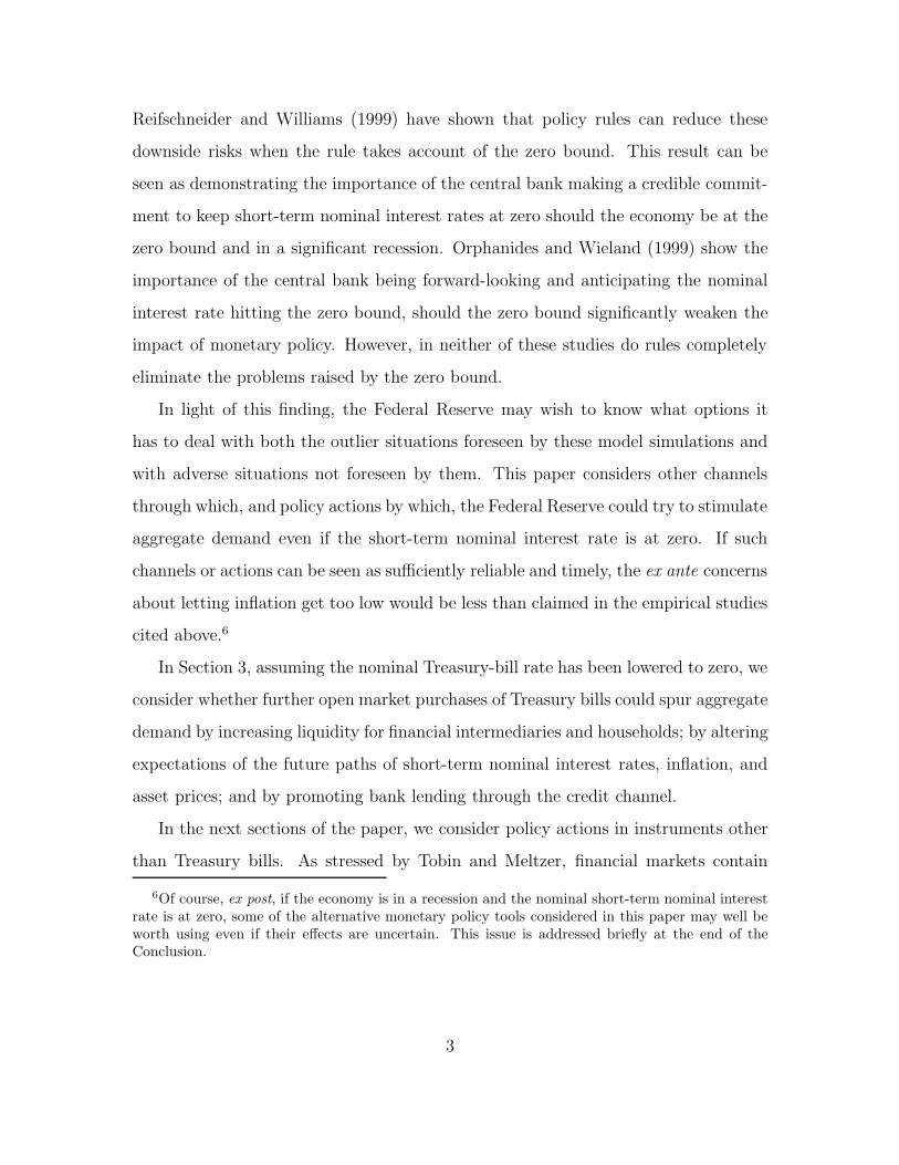
In light of this finding, the Federal Reserve may wish to know what options it

has to deal with both the outlier situations foreseen by these model simulations and

with adverse situations not foreseen by them. This paper considers other channels

through which, and policy actions by which, the Federal Reserve could try to stimulate

aggregate demand even if the short-term nominal interest rate is at zero. If such

channels or actions can be seen as sufficiently reliable and timely, the ex ante concerns

about letting inflation get too low would be less than claimed in the empirical studies

cited above.6

In Section 3, assuming the nominal Treasury-bill rate has been lowered to zero, we

consider whether further open market purchases of Treasury bills could spur aggregate

demand by increasing liquidity for financial intermediaries and households; by altering

expectations of the future paths of short-term nominal interest rates, inflation, and

asset prices; and by promoting bank lending through the credit channel.

In the next sections of the paper, we consider policy actions in instruments other

than Treasury bills. As stressed by Tobin and Meltzer, financial markets contain

6Of course, ex post, if the economy is in a recession and the nominal short-term nominal interestrate is at zero, some of the alternative monetary policy tools considered in this paper may well beworth using even if their effects are uncertain. This issue is addressed briefly at the end of theConclusion.

3

many assets that are imperfect substitutes for the monetary base and Treasury bills.7

Purchases of such assets by the Federal Reserve might lower their rates of return and

thereby stimulate aggregate demand even if the Treasury bill rate was at zero.8

First, we consider the purchase of Treasury bonds and the writing of options

on Treasury securities—actions that might be able to lower expected future short-

term interest rates and risk premiums. These policy actions are addressed in Section

4, although in Section 2 we provide some historical background for this analysis

by showing that both in the United States during the Great Depression and more

recently in Japan when short-term nominal rates were at or near zero, the yield

curve was quite steep at times and may have hindered economic recovery. Section 5

considers intervention in markets for foreign exchange, which involves purchases of

foreign-currency bills.

The Federal Reserve could also provide stimulus to aggregate demand either by

purchasing U.S. agency or private-sector debt (Section 6) or by extending loans in

which such debt was used as collateral (Section 7). In both types of operations, the

Federal Reserve Act limits the actions of the Federal Reserve. For example, there is

no express authority for the Federal Reserve to purchase corporate bonds or equities.

And in making loans, the Federal Reserve seems to be restricted in taking onto its

balance sheet the credit risk of private-sector nondepository entities.9 With only a few

exceptions, we do not consider policy actions that are not currently authorized by the

Federal Reserve Act but that might be useful to have authorized should short-term

nominal interest rates be at zero, even though past changes in the Federal Reserve

Act were spurred by economic conditions.10

7See Tobin (1982) (Tobin’s Nobel Lecture) and Meltzer (1999)8These issues are also examined by Lebow (1993).9The limits that the Federal Reserve Act places on the monetary policy actions of the Federal

Reserve are discussed in more detail in Small and Clouse (2000).10As stated by Howard Hackley (1973), who served as General Counsel to the Board of Governors

of the Federal Reserve System,

4

Finally, we consider increases in the monetary base brought about by transfers

of base money to the private sector either directly (i.e. through “money rains”) or

indirectly through tax cuts as a means to increase private-sector wealth and thereby

stimulate aggregate demand. Restrictions in the Federal Reserve Act all but rule out

“money rains” by the Federal Reserve.

Before starting the analysis of policy actions, Section 2 reviews the history of

nominal interest rates in the United States from 1865 to the present for evidence that

the zero bound has constrained policy in the past. That section also shows some

similarities in the behavior of the yield curves during the Great Depression in the

United States and currently in Japan.11

It would be unrealistic to ignore the fact that the purposes of the Federal ReserveAct were essentially of an economic nature and that changes in the law have beenoccasioned by changes in economic conditions or economic thinking. For example, itwas a drop in farm prices following World War I and an acute demand for agriculturalcredit that led to amendments to the statute in 1923 to liberalize the authority of theReserve Banks to discount agricultural paper. It was a movement to promote foreigntrade that led to a broadening of the authority to discount bankers’ acceptances; andit was the depression of the early 1930’s that prompted drastic amendments to thelaw to provide Federal Reserve credit to non-member banks and business enterprises.(Page 5.)

11Section 2 discusses the recent economic conditions in Japan but not what alternative monetarypolicy actions the Bank of Japan might undertake to stimulate aggregate demand. However, in othersections of the paper we do discuss how actual or proposed policy actions by the Bank of Japancompare with the ones we are considering for the United States. See footnotes 67 and 79.

5

2 Experiences Historically in the United States

and Recently in Japan

This section reviews the behavior of nominal interest rates in the United States histor-

ically and in Japan currently for evidence of possible constraints on monetary policy

due to the zero bound. For the United States, we also look at the 1953-1965 period

when inflation and nominal interest rates were very low, but the zero bound was

not an impediment to monetary policy and economic performance was very good on

average.

2.1 U.S. Interest Rates since the Civil War

Figure 2.1 provides an overview of U.S. interest rates since 1856. The top panel shows

yields on three-month Treasury rates since 1920 (solid line) and a high-grade private

rate of comparable maturity prior to 1936 (dashed line).12 The bottom panel shows

the composite yield on Treasury bonds with maturities of ten years or greater from

1920 to the present (solid line) and a private rate prior to 1936 (dashed line).13

The behavior of nominal interest rates since the Civil War broadly defines three

periods: (a) the period until the Great Depression, during which nominal short-term

interest rates remained well above zero as did longer-term rates, (b) the 1930s and

1940s, a period during which short-term interest rates fell nearly to zero but longer-

term rates were down only slightly from their earlier levels, and (c) the period from

the 1950s to the present when short-term rates rose well above zero and longer-term

12From 1920Q1 to 1930Q4, the solid line is the yield on three to six-month Treasury notes andcertificates. After 1930, it reflects Treasury bill rates. The dashed line is the commercial paper ratein New York City from Macauley (1938) (60-90 days until 1923Q4, four to six month thereafter).On average, it is 113 basis points higher than the Treasury rate shown in the figure during the1920Q1-1936Q4 period when the two series overlap.

13The dashed line reflects an index of high-grade railroad yields constructed from bonds withmaturities generally exceeding ten years. This series is the adjusted index number constructed byMacauley (1938) to eliminate the “long time economic drift” due to secular changes in the quality ofthe bonds. It averages 58 basis points more than the Treasury yield rate shown in the figure duringthe 1920Q1-1936Q4 period when the two series overlap.

6

0

4

8

12

16

1860 1880 1900 1920 1940 1960 1980 2000

Percent

3 Month T-Bill: 1920 - 1998Commercial Paper Rates, New York City: 1856 - 1936

Figure 2.1

U.S. Interest Rates: 1856-1998

Short-Term Rates

0

4

8

12

16

1860 1880 1900 1920 1940 1960 1980 2000

Percent

10 Year Treasury Yield: 1920 - 1998American Railroad Bond Yields, High Grade: 1856 - 1936

Yield on Long Bonds

7

rates increased by similar magnitudes.

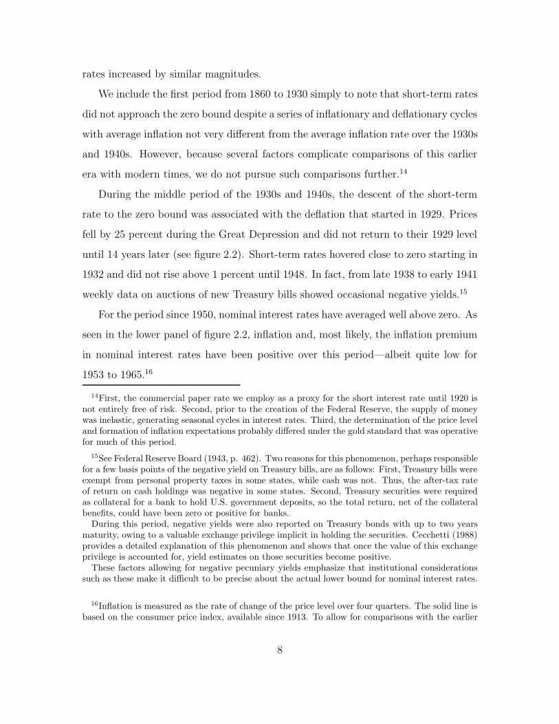
We include the first period from 1860 to 1930 simply to note that short-term rates

did not approach the zero bound despite a series of inflationary and deflationary cycles

with average inflation not very different from the average inflation rate over the 1930s

and 1940s. However, because several factors complicate comparisons of this earlier

era with modern times, we do not pursue such comparisons further.14

During the middle period of the 1930s and 1940s, the descent of the short-term

rate to the zero bound was associated with the deflation that started in 1929. Prices

fell by 25 percent during the Great Depression and did not return to their 1929 level

until 14 years later (see figure 2.2). Short-term rates hovered close to zero starting in

1932 and did not rise above 1 percent until 1948. In fact, from late 1938 to early 1941

weekly data on auctions of new Treasury bills showed occasional negative yields.15

For the period since 1950, nominal interest rates have averaged well above zero. As

seen in the lower panel of figure 2.2, inflation and, most likely, the inflation premium

in nominal interest rates have been positive over this period—albeit quite low for

1953 to 1965.16

14First, the commercial paper rate we employ as a proxy for the short interest rate until 1920 isnot entirely free of risk. Second, prior to the creation of the Federal Reserve, the supply of moneywas inelastic, generating seasonal cycles in interest rates. Third, the determination of the price leveland formation of inflation expectations probably differed under the gold standard that was operativefor much of this period.

15See Federal Reserve Board (1943, p. 462). Two reasons for this phenomenon, perhaps responsiblefor a few basis points of the negative yield on Treasury bills, are as follows: First, Treasury bills wereexempt from personal property taxes in some states, while cash was not. Thus, the after-tax rateof return on cash holdings was negative in some states. Second, Treasury securities were requiredas collateral for a bank to hold U.S. government deposits, so the total return, net of the collateralbenefits, could have been zero or positive for banks.

During this period, negative yields were also reported on Treasury bonds with up to two yearsmaturity, owing to a valuable exchange privilege implicit in holding the securities. Cecchetti (1988)provides a detailed explanation of this phenomenon and shows that once the value of this exchangeprivilege is accounted for, yield estimates on those securities become positive.

These factors allowing for negative pecuniary yields emphasize that institutional considerationssuch as these make it difficult to be precise about the actual lower bound for nominal interest rates.

16Inflation is measured as the rate of change of the price level over four quarters. The solid line isbased on the consumer price index, available since 1913. To allow for comparisons with the earlier

8

1

2

4

8

16

1860 1880 1900 1920 1940 1960 1980 2000

Ratio Scale

U.S. Prices and Inflation: 1860 - 1998

Price Level

-20

-10

0

10

20

30

1860 1880 1900 1920 1940 1960 1980 2000

Percent

Note: The solid line reflects the consumer price index, available since 1913. The dashed line from 1860 to 1933 is a cost of living index. Both price levels were normalized to equal 1 in 1913.Note: The solid line reflects the consumer price index, available since 1913. The dashed line from 1860 to 1933 is a cost of living index. Both price levels were normalized to equal 1 in 1913.

Figure 2.2

Inflation Over 4 Quarters

9

Even though the 1930s and 1940s stand out because of the low short-term interest

rates, long-term interest rates during this period were not unusually low, as seen in

the lower panel of figure 2.1. Longer-term rates can be held up by expectations of

rising short-term rates (elevated in part because short-term rates can only increase

when they are at zero) or by a positive risk premium.17 As seen in the top panel of

figure 2.3, the spread between the ten-year Treasury bond yield and the three-month

Treasury bill rate rose rather sharply at the onset of the Great Depression in 1929

and remained at a relatively high level throughout the 1930s.

The lower panel gives estimates of the Treasury yield curve at three dates.18 At

the end of 1929, as the economy was entering the Great Depression, the term structure

of interest rates, the uppermost line in the figure, was essentially flat. The short end

of the term structure moved down towards zero by the end of 1932, but the long

end remained virtually unchanged. The steepness of the curve at maturities between

one and four years in 1932:Q4 suggests that the near-zero short-term interest rates

at that time may not have been expected to persist for long. But short rates did

remain near zero and, as expectations of short-rates staying low apparently firmed,

longer-term rates slowly drifted downwards and the term spread narrowed, helping

to boost economic growth. By 1936, the yield curve was no longer unusually steep as

yields on maturities as long as three years fell to below one percent. As shown by the

shaded region in the figure, for the remainder of the decade (and longer) the yield

period, we also plot data for a cost of living index from 1860 to 1933. This is the “Index of theGeneral Price Level” series from the NBER historical database. The Reports Department of theFederal Reserve Bank of New York is listed as the original source of these data.

17In his famous interpretation of the Keynes’s General Theory, Hicks (1937) restated this keyelement of the liquidity trap as follows:

If the costs of holding money can be neglected, it will always be profitable to hold moneyrather than lend it out, if the rate of interest is not greater than zero. Consequently therate of interest must always be positive. In an extreme case, the shortest short-termrate may perhaps be nearly zero. But if so, the long-term rate must lie above it, forthe long rate has to allow for the risk that the short rate may rise during the currencyof the loan, and it should be observed that the short rate can only rise, it cannot fall.

18The data are quarterly averages of the monthly term-structure estimates in Cecchetti (1988).

10

-2

0

2

4

6

1930 1940 1950 1960 1970 1980 1990

Percent

Figure 2.3

U.S. Yield Curve

Ten-Year Treasury Bond Yield Minus Three-Month Treasury Bill Rate

-1

0

1

2

3

4

5

6

0 2 4 6 8 10

Percent

Maturity in YearsNote: The shaded region reflects the range within which the term structure fluctuated from 1937:1 - 1941:4.Note: The shaded region reflects the range within which the term structure fluctuated from 1937:1 - 1941:4.

Selected Treasury Yield Curves

1932:4

1936:4

1929:4

11

curve moved within only a fairly narrow band,

Quality spreads on private debt might have been another factor inhibiting eco-

nomic recovery when the Federal Reserve had decreased nominal short-rates to zero.

To evaluate this possibility, figure 2.4 plots quality spreads for commercial paper (top

panel) and corporate bonds (bottom panel). As can be seen, such spreads did rise

considerably during the Great Depression.

Together, figures 2.3 and 2.4 indicate two dimensions along which the Federal

Reserve could potentially provide stimulus to aggregate demand even if short-term

nominal interest rates are zero: by flattening the Treasury yield curve and by reducing

the spreads of private-sector rates over Treasury rates. These possible effects are

examined in sections 4 and 6, respectively.

2.2 Historical Review of the Policy Buffer in the United

States

While policymakers may have a variety of interest rates and rate spreads they may

attempt to affect, monetary policy becomes weakened in the first event by short-term

nominal rates hitting zero. Accordingly, we now focus on those historical periods in

which the zero bound on short-term rates was potentially seen by policymakers as

a problem. To do so, we consider from a historical perspective the amount of room

that has been available to reduce nominal rates in response to shocks.

As our measure of this “policy buffer”, we use the nominal 3-month Treasury bill

rate at the onset of recessions.19 An alternative measure is the “equilibrium buffer”—

the nominal interest rate that would prevail in equilibrium when inflation is at the

Federal Reserve’s target rate of inflation and the real interest rate is at its equilibrium

level. Starting from equilibrium, it is the room available to lower nominal short-term

interest rates in response to shocks to the economy. For our historical study, we do

19We do not use the federal funds rate because the funds market did not become well developeduntil the 1950s. See Stigum (1990), pages 366–370.

12

0

1

2

3

4

1930 1940 1950 1960 1970 1980 1990

PercentSpread Between Three-Month Commercial Paper and Three-Month Treasury Bill Rates

0

2

4

6

8

1930 1940 1950 1960 1970 1980 1990

Percent

Figure 2.4

U.S. Quality Spreads

Spread Between Long-Term Corporate and Ten-Year Treasury Bond Yields

Aaa RatingBaa Rating

13

not have accurate measures of either the Federal Reserve’s inflation target or the

equilibrium real interest rate–especially for the earlier years in our analysis, so we use

the actual nominal funds rate to measure the policy buffer.

This measure of the policy buffer needs to be interpreted cautiously, however.

At least during the 1960s, 1970s, and 1980s, the level of the nominal short-term

interest rate leading up to a recession often reflected a considerable policy tightening

undertaken to combat an upward trend in inflation. In such cases, our measure of the

policy buffer may be especially high relative to the equilibrium buffer. Similarly, the

levels in nominal interest rates during the subsequent recessions may have been lower

that would have been called for solely to offset shocks: Interest rates were lowered to

offset the weakness in economic activity that was induced to control inflation.

The top panel of figure 2.5 shows the nominal 3-month Treasury bill rate from 1929

to the present (thin line). The shaded bars cover the periods of recessions, and their

height shows our measure of the policy buffer at the start of each recession. Within

these shaded bars, the thick lines show the extent of the actual easing during the

recession—i.e. the cumulative change in the nominal interest rate from the beginning

of each recession. For example, during the 1990 recession, policy started out with

room to ease of about 7 percentage points but used only about 2 percentage points.

In the lower panel of figure 2.5, we show the same shaded bars, but replace the

nominal measures of the level of interest rates and of the easings in interest rates with

their real counterparts, using the nominal rate less actual inflation as a proxy for real

interest rates.

As is apparent in the upper panel of figure 2.5, the Great Depression stands out

not because of relatively little room for easing at the outset of the downturn in 1929

but for ultimately running out of room despite the initial room to ease. Although

the nominal short rate was falling, it was not falling as fast as the rate of inflation,

causing our estimate of the real short-rate to rise (bottom panel). This rise in the

estimated real interest rate came at a time when the level of the real interest rate

14

-15

-10

-5

0

5

10

15

20

1930 1940 1950 1960 1970 1980 1990 2000

Percent

Figure 2.5

Room for Easing During U.S. Recessions

Three-Month Treasury Bill Rate

-20

-15

-10

-5

0

5

10

15

1930 1940 1950 1960 1970 1980 1990 2000

Percent

Note: The height of the shaded regions shows the room to ease at the start of each recession. The vertical lines reflect NBERturning points. The horizontal lines shown at every recession indicate the maximum drop in the short rate that would occurduring the recession. The thick lines show the interest rate movements during the recession relative to the levelat the beginning of the recession.

Note: The height of the shaded regions shows the room to ease at the start of each recession. The vertical lines reflect NBERturning points. The horizontal lines shown at every recession indicate the maximum drop in the short rate that would occurduring the recession. The thick lines show the interest rate movements during the recession relative to the levelat the beginning of the recession.

Treasury Bill Rate Less Inflation

15

consistent with stable unemployment was surely falling.

The upper panel also shows that each of the three recessions following the Great

Depression—1937, 1945, and 1948—started in an environment of very low interest

rates, arguably near the zero bound. Going into these recessions, the room for policy

easing was a mere 44, 38 and 114 basis points, respectively. However, the recessions

were relatively short lived and the maximum extent of easing was just 38 basis points

(1937 recession). By contrast, the cumulative easing during seven out of the eight

subsequent recessions was larger than could have been accommodated by any of the

policy buffers at the start of the recessions of 1937, 1945 and 1948.

As shown, the inability to effect a substantial reduction in the short nominal rate

is reflected by an increase in the real interest rate during the low-inflation recessions

of 1937, 1945 and 1948. By contrast, our measure of the real interest rate falls during

each of the subsequent eight recessions.20

An environment of very low inflation does not necessarily imply that the Federal

Reserve will be constrained by the zero bound if a recession occurs. Along these

lines, it is useful to examine the recessions during the 1950s and early 1960s when

CPI inflation averaged about 1-1/2 percent, as shown in the top panel of figure 2.6.

The policy buffers at the beginning of the recessions of 1953, 1957 and 1960 were not

very large, 196, 335 and 299 basis points respectively. Yet, the Federal Reserve did

not experience any difficulties in engineering a turnaround in any of those recessions.

The short rate was reduced during the course of each recession, with interest rates

20Special circumstances surrounding the 1937, 1945 and 1948 recessions, however, introduce diffi-culties in directly comparing them to subsequent recessions. In 1945 and 1948, the transition from awar-time economy ought to be factored in. The 1937 recession presents a rather intriguing problemin that some scholars suggest that a contributing factor was a pair of increases of reserve require-ments by the Federal Reserve. (For example, see Chandler (1971, p. 310–20).) Federal Reserveofficials apparently became concerned that excess reserves held in the banking system presented aninflationary risk and sought to remove them. Following the second increase, however, bank lendingunexpectedly declined, reflecting perhaps that the stock of excess reserves decreased below the levelsdesired by banks for liquidity purposes. It is not clear that a low inflation target raised the likelihoodof such an error. However, one reason for setting the inflation target above zero might be to providesome room to correct serious policy errors.

16

0

1

2

3

4

5

1950 1951 1952 1953 1954 1955 1956 1957 1958 1959 1960 1961 1962 1963 1964 1965 1966

Percent

3 Month T-Bill10 Year Treasury Yield

Figure 2.6

U.S. Inflation, Interest Rates, and Output Growth: 1950-1965

Interest Rates (Quarterly Average)

0

2

4

6

8

10

1950 1951 1952 1953 1954 1955 1956 1957 1958 1959 1960 1961 1962 1963 1964 1965 1966

Percent

CPI Inflation Over 4 Quarters

Average (1952-1965): 1.40

0

5

10

15

1950 1951 1952 1953 1954 1955 1956 1957 1958 1959 1960 1961 1962 1963 1964 1965 1966

Percent

Output Growth Over 4 Quarters

Average (1952-1965): 3.74

17

at the trough reaching lows of 79, 96 and 235 basis points respectively, as indicated

in middle panel of figure 2.6. The economy rebounded without the need for further

reductions in interest rates.

Moreover, as shown in the lower panel, real growth was quite high on average

over this period, perhaps aided by the stable price environment. However, by the

end of the first two recessions the Federal Reserve would have had only limited room

for interest rate reductions in the event the economy faced adverse developments, for

example, of the sort that induced the Federal Reserve to reduce rates substantially

in the early stages of the expansion that began in 1991.

18

2.3 The Recent Economic Situation in Japan

Japan provides a more recent example of the possible implications of the zero bound.

From a monetary policy perspective, the Japanese economy during the 1990s bears a

resemblance to the U.S. economy during the 1930s. Figure 2.7 provides a summary

overview. At the start of the 1990s, the Japanese economy was clearly overheated, but

GDP growth (shown in the top-left panel) slowed in 1991 and the economy remained

stagnant until well into 1995. As shown in the top-right panel, inflation fell from

about 3 percent in 1991 to below zero by 1995.

As shown in the bottom-left panel, the Bank of Japan eased monetary policy

considerably during the period, lowering the discount rate to 50 basis points in 1995.

Arguably, deflation coupled with the proximity to the zero-bound constraint limited

the BOJ’s flexibility to reduce short-term interest rates, once the discount rate reached

its current level. On the other hand, it is not clear that any further reductions were

necessary based on conditions at that time. Indeed, the easing of monetary policy

coupled with fiscal stimulus allowed the economy to begin to recover by late 1995,

and growth picked up considerably during 1996.

During 1997 and 1998, however, the Japanese economy has experienced several

developments that made the zero bound a potential limitation on monetary policy.

First, domestic demand weakened following an increase in the consumption tax in

early 1997 and a sharp contraction of public investment in 1997. Demand also suf-

fered as consumer and business confidence fell amid concerns about how the ongoing

problems in Japan’s financial sector would be resolved. Second, the Asian economic

crisis added to deflationary pressures on the Japanese economy and worsened the

outlook for net export growth.

The deterioration of prospects for economic recovery in the face of the new crisis

increased the horizon over which short-term interest rates could be reasonably ex-

pected to remain near zero. As evidence, by the middle of 1998, yields on Japanese

government bonds with maturities as long as six years fell to under 1 percent (bottom-

19

-2

0

2

4

6

8

1990 1992 1994 1996 1998

GDP Growth

(Year/Year)Percent

0

2

4

6

8

10

1990 1992 1994 1996 1998

Interest Rates

Percent

Discount Rate3-month CD Rate10-year Bond

-2

-1

0

1

2

3

4

5

1990 1992 1994 1996 1998

Inflation

(12-month Percent Change)Percent

CPI (1990:Jan. - 1999:July)GDP Deflator (1990:Q1 - 1999:Q2)

0

1

2

3

4

5

6

7

1 2 3 4 5 6 7 8 9 10

Percent

0

1

2

3

4

5

6

7

1 2 3 4 5 6 7 8 9 10

Percent

0

1

2

3

4

5

6

7

1 2 3 4 5 6 7 8 9 10

Yield Curves(End of Period)

Percent

Figure 2.7

Japanese Economic Data

1995:12

1998:51991:12

20

right panel). Such yields were even lower than the lowest yields on U.S. government

bonds with comparable maturities during the 1930s.

Despite the depressed level of aggregate demand in Japan, short-term nominal

rates remained a bit above zero until early 1999. In February of 1999, the Bank of

Japan launched its zero interest rate policy by which it lowered the overnight call rate

to virtually zero. As noted in its public statement on September 21, 1999, in order

to keep the call rate at about zero “the Bank is continuing to provide funds in the

amount of some 1 trillion yen more than required reserve (on average about 4 trillion

yen daily).”

The delayed decline in long-term yields was similar to the experience of the United

States in the 1930s. This is illustrated by the bottom-right panel, which shows the

term structure of Japanese government bonds on three selected dates.21 When the

economy was slowing at the end of 1991, the term structure of interest rates was

essentially flat. While the short end of the term structure moved towards zero by the

end of 1995, the long end followed only to a lesser degree. But, as the economy’s health

deteriorated during 1997, longer-term rates dropped further. By the middle of 1998,

the term structure became quite flat for maturities up to three years, suggesting that

the market expect short-term interest rates to remain close to zero, and for the zero

bound, therefore, to remain relevant, for quite some time.22 As shown in the lower

left panel of Figure 2.7, the 10-year government bond rate generally has fluctuated

between 1.5 and 2 percent so far during 1999.

21The data reflect constant-maturity yield quotes from Bloomberg, smoothed using the Nelsonand Seigel term-structure model.

22In Japan, short-term interest rates on government debt and some inter-bank lending becameslightly negative in late 1998. These negative rates apparently reflected concerns about the financialconditions of Japanese banks and the convenience factor of holding liquid government bills. SeeZuckerman and Mogi (1998) and WuDunn (1998).

21

3 Increasing the Monetary Base

This section considers the potential for stimulating aggregate demand by increasing

the monetary base even after the Treasury-bill rate reaches zero. We consider only

those increases in the monetary base that are brought about by open market purchases

of Treasury bills. Of course, the monetary base may be increased by the purchase of

other assets, including those whose nominal interest rates are positive even when the

Treasury bill rate is at zero—such as Treasury bonds or other interest-bearing assets.

Purchases of such assets would have the effects due to increasing the monetary base

considered in this section. In addition, purchases of other assets may well have effects

on the rates of returns and prices of those assets and, in the case of foreign exchange,

the exchange rate.23 These possible additional effects are examined in the following

sections of this paper.24

When the Treasury bill rate is zero, Treasury bills and the monetary base are

perfect substitutes from the point of view of private-sector portfolio demands: It is

only their sum that matters for portfolio equilibrium.25 Although an open market

purchase of Treasury bills changes the composition of the holdings of Treasury bills

and monetary base, it does not change the sum. As a result, such open market

operations do not change Treasury-bill rates rates because they do not cause an

23Mishkin (1996) also considers open market operations in assets other than Treasury bills andthe effect those purchases can have both by increasing liquidity per se and by affecting longer-terminterest rates and asset prices, stating:

Expansionary monetary policy to increase liquidity in the economy can be conductedwith open market purchases which do not have to be solely in short-term governmentsecurities. This increased liquidity helps to revive the economy by raising general pricelevel expectations and by reflating other asset prices which then stimulate aggregatedemand through the channels outlined here. (See page 23.)

24Additionally, increases in the monetary base accomplished by direct transfers of base money tothe public, without the Federal Reserve receiving any compensation in exchange, could also stimulateaggregate demand. Such “money rains” and other means by which a central bank might attempt toincrease private-sector wealth are discussed in section 8.

25See footnote 1 for a discussion of the demands for money and Treasury bills when the Treasurybill rate is zero.

22

initial portfolio disequilibrium.26

When the Treasury bill rate already is at zero, open market purchases of Treasury

bills also have no direct effect on the public’s wealth. The public’s increased holding

of the monetary base is offset by the decline in the value of their holdings of Treasury

debt and, because the Treasury bill rate cannot be reduced any further, there are

no potential capital gains on Treasury bill holdings.27 With no direct wealth effect

and the short-term Treasury bill rate unchanged (at zero), any stimulus to aggregate

demand generated by purchases of Treasury bills would have to result from other

effects; such as effects on liquidity, expectations, or through the credit channel.

3.1 Increases in Liquidity

With continued purchases of Treasury bills, the Federal Reserve injects additional

reserves into the banking system. In rather mechanical “multiplier” models of money

creation, the provision of additional reserves reliably leads to expansions in loans,

deposits, and both narrow and broad measures of the money supply. But, as noted

by Tobin (1963), these multiplier effects are too simple as a description of how banks

operate in competitive markets in which they compete for deposits and optimize their

26This point has been stressed by Meltzer (1999).27If Ricardian equivalence is assumed to hold, the decrease in the public’s wealth due to the decline

in their holdings of government debt is offset by a decrease in their future tax liabilities that wouldbe needed to finance the debt. (The Treasury does not need to levy taxes to pay the interest onthe Treasury debt that the Federal Reserve purchases because the Federal Reserve turns over to theTreasury the income that it receives from that debt.) The net wealth of the public increases by theamount of the increase in the monetary base. If prices are sticky in the short-run, then the increasein the stock of the nominal monetary base initially increases real wealth, providing a stimulus toaggregate demand.

If the nominal interest rates at which the Treasury finances its debt are zero forever, the govern-ment need not ever raise taxes to finance the publicly held debt (the face value of the debt can berolled over), so the decline in the public’s holdings of Treasury bills is not offset by a decreased taxliability. But if one assumes that at some future time the Treasury’s financing rates rise and stayabove zero, then the Treasury debt held by the public has an associated tax liability. The presentvalue of the tax liability and the market value of the Treasury debt are the same if, at each maturity,the Treasury’s financing rate and the market’s discount rate are the same.

23

portfolios across alternative assets.28 At nominal interest rates of zero, depositories

still optimize their portfolios, although the short-term interest rate at zero has pow-

erful effects on the results of that optimization.

As part of their portfolio management, depository institutions equate the risk-

adjusted marginal returns across the various assets in their portfolios. On the asset

side of their balance sheets, when Treasury bills have an interest rate of zero, the

depositories adjust the quantity of loans until the risk-adjusted return on loans also

equals zero. In this equilibrium, further open market purchases of Treasury bills

cannot lower the Treasury bill rate further and therefore would not have their usual

effect of lowering the return on Treasury bills relative to loans. Consequently, banks

do not increase their desired holdings of loans. Open market purchases of Treasury

bills would simply boost the level of excess reserves.29 In essence, these open market

operations result in the exchange of Treasury bills for reserves, which we can approx-

imate as perfect substitutes for each other in these circumstances because both of

them would have an interest rate of zero and essentially no price risk or default risk.

Such open market operations do not change the desired sum of Treasury bills and

reserves that are held, they only change the composition of this sum.30

A similar argument applies to the effects of additional liquidity injected by an

open-market purchase of Treasury bills and seen as working through money de-

mand equations. In cash-in-advance, money-in-the-production-function, money-in-

28As noted by Tobin (1963), “Commercial banks do not possess, either individually or collectively,a widow’s cruse which guarantees that any expansion of assets will generate a corresponding expan-sion of deposit liabilities. Certainly this happy state of affairs would not exist in an unregulatedcompetitive financial world. Marshall’s scissors of supply and demand apply to the “output” of thebanking industry, no less than to other financial and non-financial industries.” (See page 418.)

29Likewise, reductions in reserve requirements would not stimulate loan supply but would resultonly in additional excess reserves. This is because at nominal interest rates of zero, the opportunitycost of holding excess reserves (the Treasury bill rate or the risk-adjusted return on loans) is zero.

30In cases of a “credit crunch”, the portfolio problems at financial intermediaries are not likelyto be resolved by substituting reserves for Treasury bills. The portfolio problems lay in the loansthat are under-performing or in default. These problem loans would remain on the balance sheetsif reserves were increased and Treasury-bill holdings were decreased. Furthermore, the value of theloans would be unaffected if interest rates were unchanged because Treasury bill rates were at zero.

24

the-utility-function, shopping-time models of money demand, and the ‘square root”

money demand rule of Baumol (1952), the nominal interest rate is the marginal value

of liquidity.31 When the nominal interest rate is zero, the marginal benefits from

additional liquidity (or means of payment) provided by open market operations are

also zero, and the additional liquidity per se has no effect on aggregate demand.32

3.2 Effects Through Expectations

Monetary policy traditionally is seen as having powerful effects through influencing

the expectations of future nominal interest rates, inflation, and asset prices. However,

the ability to affect these expectations comes into question if the nominal short-term

interest rate is at zero.

31These models typically do not contain an own-rate paid on money; such as rates paid on small-time, passbook saving, and OCD deposits. If these money demand models did contain these rates,the opportunity cost of holding money would not be the nominal interest rates but would be thespread of the nominal rate over the own-rate. When the T-bill rate is at zero, the opportunity costof holding deposits may not be zero, depending on the level of the own-rate paid on deposits. Weabstract from these considerations in this study.

32At zero nominal interest rates, these models exhibit what Cole and Kocherlakota (1998) call thesatiation property, which they define as the property that

For any given level of consumption, there exists a finite level of real money balancessuch that households with real balances above that level are indifferent to using moneyand bonds as a way of accumulating additional wealth if the two assets earn the samerate of return. (See page 9).

For example, in the cash-in-advance model of money demand that they use, Cole and Kocherlakotanote that, at zero nominal interest rates, the cash-in-advance demand for real balances is indeter-minate because money serves not only as a medium of exchange but is also held as a store of value.Krugman (1998a) also makes this point.

It is precisely this satiation that delivers the results in Cole and Kocherlakota (1998) and Ireland(1996) that zero nominal interest rates are optimal. In Ireland (1996), shocks to velocity can ad-versely affect aggregate demand when nominal interest rates are strictly positive, but not when theyare at zero because:

Under the Friedman rule, when the nominal interest rate is driven to zero, the rep-resentative household carries a stock of real balances that is large enough to renderinconsequential any disturbances to its transactions technology [i.e. to velocity]. Byensuring that money is not dominated by claims issued by the private financial sector[i.e. that nominal rates are at zero], the government eliminates shocks to this sectoras a source of output fluctuations. (See page 718).

25

When the short-term nominal interest rate is at the zero bound, a central bank

may have less than complete credibility that it will keep short-term rates at zero for

a prolonged period of time. As a result, expected future short-term rates and current

long-term interest rates may remain above zero—apparently such as in the United

States in 1932 during the Great Depression (figure 2.3) and in Japan during their

economic downturn in 1991 (figure 2.7).33

Increases in the monetary base brought about by open market purchases of Trea-

sury bills even after short-term nominal interest rates are at zero may demonstrate a

resolve by, and a priority of, the central bank to keep short-term rates at zero. Such

effects would almost certainly be present when short-term rates had just been driven

to zero. But these effects might wane as purchases of Treasury bills increased if, as

argued in section 3.1, the purchase of Treasury bills led mainly to higher levels of

excess reserves and the Federal Reserve was seen as unwilling to use other tools at its

disposal to influence future short-term and current long-term interest rates.

Wolman (1998), and Krugman (1998b) have suggested that aggregate demand

can be stimulated when nominal short-term interest rates are at zero by having the

central bank drive real interest rates lower by increasing inflation expectations. At

issue are the channels through which monetary policy is expected by the public to

affect expectations of future inflation.

The analysis by Wolman (1998) is explicit in modeling how the Federal Reserve

could rely on inflation expectations to adequately affect real interest rates when nom-

inal rates are at zero. In his analysis, with prices set optimally by firms and the

Federal Reserve targeting the price level:

monetary policy can offset the zero bound by generating temporary ex-pected inflation. With real rates thus unconstrained, the existence ofthe zero bound does not appear to constitute an argument against a low

33As expectations of future short-rates approach the lower bound of zero, progressively more ofthe lower end of the distributions of future short rates becomes truncated by the zero bound. Theassociated risk of capital losses on bonds increases and works to keep bond rates above zero.

26

inflation target.34

This flexibility in inflation expectations is strengthened by a Federal Reserve policy

rule that targets the level of prices. Weakness in aggregate demand will cause the

price level to fall below its targeted level. But, going forward, markets will expect

some temporary inflation as the price level rises to its targeted level.

For this analysis, as well as others that depend on the Federal Reserve affecting

expectations of inflation, a key issue is whether the Federal Reserve has tools by which

it can credibly increase current or future inflation (and, therefore, current inflation

expectations) even if short-term nominal interest rates are zero. The monetary policy

tool used by Wolman is a money rain. The injections of money relax the representative

households’ budget constraint and thereby stimulate aggregate demand. Because the

households are rational and know the structure of the monetary policy rule, they can

accurately anticipate that the rule, with its associated money rains, will ultimately

drive the price level to its targeted level if an economic downturn initially pushed the

price level below its targeted level.

Krugman (1998b) also has a proposal based on increasing inflation expectations.

For the currently weak Japanese economy, he has suggested:

The way to make monetary policy effective, then, is for the central bankto credibly promise to be irresponsible—to make a persuasive case that itwill permit inflation to occur, thereby producing the negative real interestrates the economy needs. (See section 6 of Krugman (1998b).)

In his analysis, Krugman ensures that monetary policy can stimulate the economy

even when the Treasury bill rate is at zero by assuming that wage and price rigidities,

and therefore the liquidity trap, are temporary. Markets anticipate the future return

to positive nominal interest rates, and this anticipation is a fulcrum with which to

affect current market expectations. The central bank simply has to convince the

public that it will use this return to flexible prices and positive nominal interest rates

34Wolman (1998), page 17.

27

to raise the future level of prices—thereby raising current inflation expectations and

lowering current real interest rates. To do so, the central bank increases the current

stock of money. If the increase was temporary, it would have no effect on aggregate

demand. But the central bank credibly promises that this increase will persist into

those future periods in which nominal short-term interest rates would have returned

to being positive.35 The expected potency of monetary policy in those future periods

raises the price level currently expected for those periods—raising current expected

inflation.

This expectation that policy will be effective in future periods can be used to

stimulate aggregate demand even if prices and inflation expectations adjust sluggishly.

Current prices on assets could adjust immediately to the expectation that monetary

policy will be more expansionary in future periods. Bond and equity prices could

rise, and the dollar could depreciate.36 In essence, forward-looking expectations by

the public have the effect of bringing into the present the expected power of future

monetary policy.

But an unfortunate aspect of the zero bound is that the worse the current economic

downturn, the longer may be the period over which nominal short-term interest rates

are expected to remain at zero, and the further into the future until the central bank

can use its standard tools to stimulate aggregate demand. In other words, the worse

the recession, the larger may be the monetary policy action needed to achieve a given

marginal stimulus to aggregate demand.

3.3 Effects Through the Credit Channel

Bernanke and Gertler (1995) have argued that the traditional view sees monetary

35Theoretically, put options on interest rates, discussed in section 4.3.1, could be written by theFederal Reserve such that reserves are automatically injected in those periods when interest ratesturn positive. Small and Clouse (2000) discuss what legal authority the Federal Reserve has toengage in options.

36Orphanides and Wieland (1999) consider such effects on exchange rates and their implicationsfor monetary policy.

28

policy as having its effects mainly through interest rates, but that this view does

not seem to fully explain the observed potency of monetary policy. They argue that

monetary policy derives much of its power to affect aggregate demand from imperfect

information and other “frictions” in credit markets. Of interest then is whether open

market operations can provide stimulus through the credit channel even when short-

term nominal interest rates are at zero.

As Bernanke and Gertler indicate, the credit channel seems to require changes in

market interest rates:

We don’t think of the credit channel as a distinct, free-standing alternativeto the traditional monetary mechanism, but rather as a set of factors thatamplify and propagate conventional interest rate effects.

In particular, Bernanke and Gertler see the credit channel as working through

two main linkages between monetary policy and the magnitude of lending in financial

markets. The balance sheet channel stresses the importance of firms’ and households’

balance sheets and income statements. An easing of monetary policy spurs credit

flows by improving the financial health of firms and households—typically through

decreasing interest expenses or increasing asset prices. However, when short-term

interest rates are already at zero, continued open market purchases of Treasury bills

would not directly affect either of these two indicators of financial health—although

they could affect these indicators through some of the other channels discussed in this

section.

A second linkage between monetary policy and credit flows is provided by the

bank lending channel. This linkage relies on monetary policy affecting the supply of

bank loans. As argued above, when nominal interest rates are at zero, the continued

injection of liquidity through open market operations in Treasury bills would not be

expected to shift a bank’s desired portfolio allocation towards loans and away from

excess reserves and Treasury bills. The bank lending channel also stresses that any

monetary policy action that lowers the cost of funds to a bank would lead to increases

29

in the size of bank portfolios, and to an increase in loans in particular. However, with

the nominal short-term interest rate already at zero, there seems to be no obvious

scope for additional open market operations in Treasury bills to directly lower the

cost of funds.

Nonetheless, the credit channel may well remain important for reviving aggregate

demand should the economy be in a zero-bound recession. If open market opera-

tions in assets other than Treasury bills are effective in lowering interest rates on

those assets (as discussed in the sections below), the credit channel can amplify and

propagate those interest rate changes. Also, if a credit-crunch is present at the zero

bound, regulatory reform of and financial aid to depositories may provide stimulus to

aggregate demand through the credit channel.

30

4 Policy Actions in Longer-Term Treasury Securi-

ties and in Options on Treasury Securities

As shown in Section 2, historical experience in the United States and recent experience

in Japan suggest that longer-term nominal interest rates may remain elevated and

thereby hinder economic recovery even when the short-term nominal interest rate is

zero. This section explores two policy actions the Federal Reserve may undertake to

reduce longer-term Treasury rates: the purchase of Treasury bonds and the writing

of options on Treasury securities.37

4.1 Open Market Operations in U.S. Treasury Bonds

If the Federal Reserve has driven the nominal short-term Treasury rates to zero,

it could switch from purchasing Treasury bills to purchasing Treasury bonds. The

effects on the monetary base are the same whether bills or bonds are purchased.38

Indeed, the purchase of Treasury bonds can be seen as being the combination of

two transactions: the open market purchase of Treasury bills and the exchange of

Treasury bills for Treasury bonds. The effects due to the increase in the monetary

base were discussed in section 3. Here we focus on possible direct effects on bond

rates.

37In this paper we do not consider open market operations in U.S. Treasury inflation-protectedsecurities (TIPS). The TIPS market is still relatively thin, and deep markets do not exist for otherinflation-indexed securities that are close substitutes for TIPS. As a result, open market operationsthat affected yields on TIPS might have little effect on other market rates. Indeed, if the FederalReserve purchased all TIPS, the structure of financial markets would merely return to the structurepresent prior to the introduction of TIPS in January of 1997.

Furthermore, if the zero-bound on nominal interest rates were binding and the economy experi-encing weak aggregate demand, the potential problem for the economy would be deflation. In thiscase, TIPS would become much like standard nominal Treasury debt because, although TIPS areindexed to inflation, TIPS are not indexed to deflation: “At maturity, the [inflation-indexed] secu-rities will be redeemed at the greater of their inflation-adjusted principal or par amount at originalissue.”Summary of Marketable Treasury Inflation-Indexed Securities (1999)

38By merely extending the maturity of the Treasury securities that it purchases, the FederalReserve need not be committing itself to increasing the monetary base for a more prolonged periodof time: The Federal Reserve could alway sell the bonds before they mature.

31

The theory of asset pricing that we employ–following Shiller (1979) and Shiller,

Campbell and Schoenholtz (1983)–equates expected holding-period returns across

traded assets, with some adjustment for differential risk premiums. For the case of

a discount bond, the current long-term interest rate is an unweighted average of the

current short-term interest rate and expected future short rates, plus a risk premium:

iLt = (1/N)

N−1∑

j=0

Et(it+j) + θLt (1)

where: iLt is the long-term bond rate at time t.

it is the short-term rate at time t.

θLt is the risk premium on long-term bonds.

The risk premium θLt is seen as being composed of two components—one reflecting

the risk that interest rates may change and the other (in the case of private-sector

securities) reflecting the credit risk associated with defaults.39

4.1.1 The Signalling Channel

If Treasury bills and bonds are perfect substitutes, reflecting risk neutrality by pri-

vate agents, both asset will be held only if their expected returns are equal (except,

perhaps, for a constant risk premium). This condition is often referred to as the

expectations theory of the term structure and is obtained by setting θLt to zero (or a

constant) in equation 1. With the risk premium unaffected by open market purchases

of bonds and with the current Treasury bill rate fixed (at zero), purchases of Trea-

sury bonds can cause the bond rate to fall if (and only if) the purchases can cause

private agents to expect the future bill rate to be lower than they expected it to be

before the bond purchases–for example, to remain at zero rather than rising above

39Koziki and Tinsley (1999) provide alternative models of the public’s perceptions of the conductof monetary policy and test how well the models can explain the behavior of the term structure ofinterest rates.

32

zero. Such effects on expected future bill rates could result from bond purchases

due to effects through the signalling channel, which was first identified in the foreign

exchange literature.40

The signalling channel assumes bond purchases will cause private agents to expect

future bill rates to be lower. Suppose the Federal Reserve buys Treasury bonds

rather than bills in an attempt to convince the public that it will deliver low short-

term nominal interest rates in the future. The value of the Federal Rerserve’s bond

holdings will be higher if it delivers lower short-term rates in the future. If market

participants know these Federal Reserve purchases are taking place, they might come

to expect that future bill rates will be lower. If they do, bond rates will have to be

lower today in order for the condition implied by the expectations theory to hold.

Bond purchases might have some effect through this “signalling effect” even if the

monetary authorities have already announced that they will keep the bill rate a zero

because after the purchases the Federal Reserve has more to lose by not carrying

through with their announced policy.

4.1.2 The Portfolio Balance Channel

Alternatively, bond purchases could affect bond rates if the purchases can change

the risk premium θLt in equation 1. Such “portfolio effects” have been described, for

example, by Tobin (1982) and Meltzer (1999). In this view of portfolio behavior,

bonds are seen as imperfect substitutes for bills because investors are risk averse and

bonds and bills have different risk characteristics or because investors have “preferred

habitats.”41 If the relative supply of assets with a preferred maturity declines (say,

because the Federal Reserve purchases them) the risk premium in the interest rate

on that assets will decrease.42

40See Mussa (1981).41See Modigliani and Sutch (1966).42We make this argument, in part, for completeness. If the Federal Reserve cannot bid down risk

premiums then it has one less way in which it can counter zero-bound recessions.

33

Portfolio balance effects are probably negligible when the (remaining time to)

maturity structure of Treasury debt is in its normal range. Perhaps this is the reason

that studies of Operation Twist, an operation undertaken in 1961, and similar small-

to medium-sized changes in the maturity composition of the government debt suggest

that such changes have little or no effect on risk premiums. However, portfolio effects

would almost certainly not be negligible if either bonds or bills became very scarce.43

Therefore, it seems almost certain that a determined Federal Reserve, willing to

absorb virtually the entire supply of Treasury bonds, could lower their interest rates

and raise their prices to some extent. For example, the Federal Reserve fixed the

yields of Treasury securities during World War II and up to the Treasury-Federal

Reserve Accord of 1951 by standing ready to buy all Treasury securities offered at

interest rates above a targeted level.44

The degree to which any such decline in Treasury rates would feed through to the

cost of credit to private borrowers is difficult to determine. The public would not only

be facing lower returns on their Treasury holdings but also would have experienced

a capital gain on them. Attempts to rebalance portfolios by buying corporate debt

would tend to reduce the return on that debt below the level dictated by expected

short-term rates (assuming they are unchanged by this action), perceptions of corpo-

rate risk, and the “normal” term premium on long-term debt, especially to the extent

Hanes (1999) presents a model in which non-bank arbitragers essentially remove all preferredhabitat considerations from the pricing of Treasury debt when the nominal interest rates on thatdebt are strictly positive. However, when the nominal Treasury-bill rate is zero, non-bank arbitragersare driven from the market for Treasuries, and banks dominate in the determination of Treasuryprices. Banks are risk averse because the price risk of bonds can adversely affect banks through thesolvency standards that they face. Hanes shows his model is consistent with patterns in bond pricesin the United States during the 1930s when short-term nominal interest rates were near zero.

43Fleming (2000) suggests that “ If projected [federal] budget surpluses materialize, they couldlead to a significant reduction in the Treasury market’s size and to a deterioration in the market’sliquidity and efficiency.”( pp. 13). Currently, participants in U.S. Treasury markets point to therevised outlook for the federal budget as a factor contributing to concerns about the future scarcityof Treasury securities. Yields on Treasury securities seem to be depressed relative to yields on similarmaturity private yields, especially at the longer end.

44See Meulendyke (1998), pages 33-35.

34

the “preferred habitats” in the holdings of Treasuries and corporate debt match one

another. How much private rates would decline will depend in part on the extent

to which bonds of U.S. corporations are close substitutes for other assets in global

financial markets. The greater the degree of such substitution, the greater the odds

that global arbitrage would limit the decline in private rates in the United States.

If there are no effects on longer-term interest rates (and short-term rates) then to

the extent the credit channel works by propagating interest rate changes (as quoted

above from Bernanke and Gertler) bond purchases would have no stimulative effect

through the credit channel. Credit-channel effects could be spurred if the purchase

of assets from a bank makes the asset side of the bank’s balance sheet more liquid.

However, such effects are likely to be weak (if present at all) because Treasury bonds

are highly liquid and the market price of liquidity (the short-term nominal interest

rate) is assumed to be at zero.

4.2 Writing Options on Treasury Securities

As noted above, one limitation to using purchases of longer-term Treasury securi-

ties to drive interest rates lower is that there is no commitment by the Federal Reserve

as to how long the securities that were purchased will be held. To help sharpen the

public’s perception of the Federal Reserve’s intended path for the future course of

interest rates and strengthen the Federal Reserve’s commitment to that path, the

Federal Reserve could find it useful to enter the markets for options on Treasury

securities.45

4.2.1 Introduction

To provide a signal that it will keep interest rates low, the Federal Reserve could

convey an upper limit to the future level of interest rates by writing option contracts.

The Federal Reserve could write options such that if interest rates rose above these

45This section borrows heavily from Tinsley (1999).

35

limits, the private-sector holder of the option would gain financially at the expense of

the Federal Reserve. By contrast, if future interest rates were below the limits, there

would be no gain or loss for either the Federal Reserve or the holder of the option

(aside from the initial price of the option).46

In essence, the Federal Reserve would be penalizing itself if interest rates breached

the upper limit, thereby providing both some commitment to keeping rates below

these limits and some “insurance” payments to option holders should the limits be

breached. In contrast, open market operations in Treasury bonds at particular prices

may be less credible because holders of bonds would not be compensated for subse-

quent departures from currently expected rates built into bond yields.

Additionally, if the options expire when interest rates are above the options’ ceiling

rate, the Federal Reserve would be adding reserves and increasing the monetary base.

Expectations of these potential reserve injections would help lower the short-term

46Small and Clouse (2000) discuss the authorization in the Federal Reserve Act under which theFederal Reserve could enter options markets. The only occasion on which the Federal Open MarketCommittee has authorized the purchase or sale of options is the temporary authorization aimedat promoting smooth functioning of money and financing markets near year-end 1999 in light ofthe potential for Y2K strains. See the September 8, 1999 press release by the Federal ReserveBank of New York, which is available on the web site of the Federal Reserve Bank of New York:www.ny.frb.org. See the “announcements” section under “news items”.

These nature of these options allowed the buyer to engage in a repo transaction with the OpenMarket Desk at a pre-specified rate set at 150 basis points above the intended federal funds rate.The options were sold in seven weekly auctions from October 20 to December 1. Only primarydealers were allowed to bid at these auctions, but they were allowed to submit bids on behalf ofcustomers. The options were structured as three one-week “strips” with the first strip covering theweek from December 23 to 29, the second strip covering the week from December 30 to January5, and the third strip covering the week from January 6 to January 12. Each strip amounted to aportfolio of options that allowed the buyer to engage in RP transactions with the Federal Reserveup to the notional quantity of the contract on any or all days in the strip.

The volume of propositions for the options, especially at the early auctions, was quite large,prompting the Desk to conduct two more auctions of options than it had originally intended. Intotal, notional quantities of $114 billion of options were sold for the week starting December 23,$223 billion for the week starting December 30, and $144 billion for the week starting January 6.As intended, the options seemed to have a significant calming effect on financial markets. Variousbutterfly spreads and other measures of Y2K-related uncertainty in financial markets peaked inOctober prior to the auctions and then dropped sharply in subsequent weeks. Market participantsnoted that the options had effectively provided them with what they perceived to be fairly low costinsurance against the possibility that financing markets would be severely disrupted over the turn.

36

rates expected to prevail when the options expire.47

To convey this signal on a ceiling for future interest rates and to provide the

commitment, insurance, and reserves injections, the Federal Reserve would be the

party to write the options and specify the strike price for the underlying Treasury

security. The strike price would be set to correspond to the particular interest-rate

ceiling the Federal Reserve wanted to convey to the market. That strike price would

correspond to an interest-rate ceiling if the contracts were written as put options.

Put options would imply an interest-rate ceiling because the private-sector holders of

put options would have an incentive to exercise the option if the market price of the

Treasury security fell beneath the strike price—i.e., if the market rate of interest were

above the rate of interest implicitly set by the Federal Reserve in the setting of the

strike price. To realize a gain in this situation, the holder of the option could purchase

the Treasury security at the “low” market price and then “put” the Treasury security

to the Federal Reserve at the higher strike price—pocketing the profit.48

4.2.2 The Writing and Pricing of Options

In writing a European option, three characteristics of the option must be specified: the

underlying instrument, the expiration date of the option, and the strike price.49 For

example, suppose put contracts are written on 9-month Treasury bills, the expiration

47Option payments by the Federal Reserve also have a fiscal policy aspect—they represent a directtransfer from the Federal Reserve to the public.

A possible additional advantage of policy options suggested by Merton (1995) is that options con-tinue to work automatically against unexpected shocks, without waiting for subsequent interventionsby the Trading Desk.

48Of course, as is the standard case in the settlement of options, instead of actual delivery of thesecurity to the Federal Reserve, a cash settlement could be undertaken.

49European options can be written only on a rate that exists at a single point in time. However,firms and households are likely to make decisions on the basis of average interest rates over a planningperiod, not interest rates at a particular point in time. One alternative is for the Federal Reserveto write average-value options, where the owner of the option is compensated for average deviationsfrom strike prices or interest rates over the length of the option rather than for the differential thatexists only at the option expiration date. For valuations of average-value options, see Turnbull andWakeman (1991) and discussion of so-called “Asian” options in Hull (1997).

37

date of the option is in three months, and the strike price equals the face value of

the bills (which we take to be $1.00) so that the implicit interest rate ceiling is zero

percent. In three months, the holders of these options will have an incentive to

exercise the options if Treasury bills can be purchased in the open market for less

than $1.00; i.e. if the interest rate on 9-month Treasury bills positive.

Table 4.1 indicates possible valuations of the 3-month call option associated with

a 9-month discount Treasury bill.50 The columns correspond to four different assump-

tions of the interest rate expectations that may be used by the market in pricing this

option.51 The rows of the table correspond to alternative “strike rates” implicit in

corresponding strike prices the Federal Reserve could specify in writing the options.

Table 4.1: The Value of 3-Month Put Options on the 9-Month Treasury Ratea

implicit Market expectations of thestrike-rates 9-month forward rate (Etr9,t+2)

b

0.1 2.0 4.0 6.0rx = 0.1 .012 1.872 3.842 5.812rx = 2.0 0.0 .244 1.974 3.940rx = 4.0 0.0 .004 .488 2.038rx = 6.0 0.0 0.0 .068 .732

aIn valuing these options we assumed that the standard deviation of log forward rate, σ9,t+2 equals 0.312and the discount factor, e−r3,t/400 equals 0.985.

bFor the sample 1982m10-1997m9, means of the 3-month zero coupon rate and the forward 9-month ratewere about 6.3 and 7.0. The standard deviation of the forward 9-month log rate was approximately 0.312.

50The valuations in table 4.1 are based on the solution developed by Black (1976). In discussingthe use of bond options, it is immaterial whether the bond option is formulated in terms of a strikeprice, such as the bond put, or in terms of a strike rate, such as the interest rate call. Differencesmay exist in practice due to expectation assumptions or institutional conventions. For example, thevaluation of an option is not invariant to alternative assumptions that the bond price or the bondinterest rate is lognormally distributed. Bond options traded in over-the-counter markets are oftenformulated in interest rate terms, whereas bond options traded in exchanges are often expressed inbond price terms.

51For simplicity, the standard deviation and 3-month discount factor are assumed to be the samefor each of the columns in Table 4.1.

38

From the table, three aspects of option prices can be seen. First, the option

has value even if the strike rate equals the market expectation of the forward interest

rate—as shown along the main diagonal in the table. The option has value because the

price of the bond has some chance of falling below the strike price—so the expected

value of the pay-out from the option is positive. This value would accrue to the

Federal Reserve when it initially sells the option in the market.

Second, the insurance aspect of the options is seen by the entries to the right of

the diagonal, where the market expectations of what the 9-month rate will be at the

time of the expiration of the option exceed the implicit strike-rate. For example, at

the far right in row one, the market expects an interest rate of 6.0 percent, the strike

rate is 0.1 percent, and the value of the option is 5.8. This positive value accrues to

the holder of the option should he sell the option when market expectations are at

the indicated rate.

And third, to the left of the diagonal when the expected rate falls below the strike

rate, the option has almost no value. In this sense the risk to the value of the option

is one sided and the option has the characteristic of insurance.

This table simplifies the determination of option prices in that it shows only how

option prices are affected by market expectations of forward interest rates. But option

prices are also affected by the market’s perceptions of the likely volatility of interest

rates. This volatility is a measure of the market’s confidence that the actual rate at

the expiration date will match the market’s current expectation of that rate.

These readings on perceived volatility can be derived from the observed option

prices if, from other sources, one can obtain measures of the expected future interest

rates. Typically, these expectations can be obtained from interest-rate futures con-

tracts. The readings on perceived volatility may be useful to the Federal Reserve as

a measure of the public’s confidence in its interest rate policy.

39

4.2.3 Using Options to Alter Market Expectations

Apart from possible effects due to improvements in the liquidity of asset markets,

the prices of the underlying assets (such as Treasury securities) are not ordinarily

expected to be altered when derivative securities are written by the private sector.52

Valuations of derivatives are based on the expected payoffs on underlying assets. In

turn, the values of these underlying assets depend on the economic fundamentals that

determine the present value of expected earnings. Apart from temporary increases in

volatility during episodes of large price movements such as October 19, 1987, there is

little empirical evidence to support a reliable causal connection going from valuations

of options to valuations of underlying assets.53

By contrast, the use of derivatives by the central bank has the potential to alter

the market’s perceptions of economic fundamentals. As noted in equation 1, two types

of expectation components are embedded in longer-term bond rates: the average of

expected short rates over the maturity of the bond, and the perceived uncertainty

of the short rate policy as priced in the term premium of bonds. With options, the

Federal Reserve could potentially affect both of these bond-rate fundamentals.

Given that the central bank has a monopoly on the supply of the domestic cur-

rency, it has the capacity to purchase any amount of outstanding Treasuries that is

necessary to fix the short-term rate in a given period. Put options written by the

Federal Reserve could provide the explicit signals as to the planned trajectory and

horizon of the short-rate intentions of policymakers. Market observers will note that

the more options that are written by the Federal Reserve, the more money would be

left on the table if the central bank walked away from its commitment to achieve the

52In principle, the existence of well-developed derivatives markets tends to reduce bid-ask spreadson underlying assets (Fedenia and Grammatikos 1992) .

53Different views on the October 1987 consequences of portfolio insurance based on dynamictrading of stocks are advanced in Hull (1997) and Mullins (1997). The latter also provides a generalreview of the empirical literature exploring effects of derivatives on asset markets.

40

interest-rate ceilings written into the option contracts.54 And any deviation above

these ceilings might be muted by the automatic reserves injection that would occur

when the options expire.

The second expectational component of bond rates is the perceived uncertainty of

the short rate policy as priced in the term premium of bonds. If market perceptions of

the future short rates designated in the put options were held with greater certainty

because of the Federal Reserve’s clearer signal about and increased commitment to

its interest rate intentions, the term premiums associated with the volatility of these

rates could decline. Additionally, for any degree of interest-rate risk, the market

might price it more modestly given the insurance aspects of the put contracts written

by the Federal Reserve.55

54Ironically, this may strengthen the credibility of option policies more for weak central banks thanfor strong central banks, if the former are not able to absorb large episodic losses. But to be sure,writing put options does not produce an ironclad commitment. The Federal Reserve could allowrates to rise and simply pay the penalty if it judged that higher rates were in the national interest.Knowledge that this was possible might limit the effectiveness of option contracts in reducing interestrates.

55Also, when the zero bound is expected to be binding at times, the reduction in perceived volatilitymay decrease the expectations of future short rates. This is because the reduced variance lowers theupper tail of the distribution of future short rates but the lower tail remains truncated at zero.

41

5 Policy Actions in Foreign Exchange

Under flexible exchange rates, the Federal Reserve could try to stimulate the econ-

omy by attempting to depreciate the dollar through intervention in foreign exchange

markets—in effect, buying foreign currency bills instead of U.S. Treasury bills.56

When the U.S. bill rate is above the zero bound, unsterilized intervention causes

more depreciation than sterilized intervention because the unsterilized intervention

lowers the bill rate. However, with a bill rate of zero, unsterilized intervention cannot

lower the bill rate and, therefore, sterilized and unsterilized intervention have the

same effects. 57

In principle, interventions can affect the exchange rate through either or both

of two channels: the signalling channel and the portfolio balance channel. These

channels can be explained using the following expression:

it = iFt + Et(st+1) − st + θDt (2)

where: it is the interest rate on U.S. Treasury bills;

iFt is the interest rate on foreign-currency bills;

st is (the logarithm of) today’s spot exchange rate,

expressed as $ per foreign currency;

Et(st+1) is the expectation of (the logarithm of the) future spot exchange rate;

θDt is the risk premium on U.S. Treasury bills.

This expression equates the yield on U.S. Treasury bills to the sum of the expected

56It is taken for granted that foreign interest rates remain unchanged. It is an open questionwhether an increase in foreign interest rates that causes a depreciation of the dollar would producea net stimulus for the U.S. economy.

57Three assumptions underlie this claim: (1) Treasury bills and the monetary base are perfectsubstitutes when the Treasury bill rate is at zero, (2) sterilization is done through the sale of Treasurybills, and (3) the economy is at a point at which increases in the monetary base brought about byopen market purchases of Treasury bills provide no further stimulus to aggregate demand. Note,in particular, that if increases in the monetary base have stimulative effects through the channelsdiscussed in section 3, then assumption (3) does not hold and unsterilized intervention will be morestimulative than sterilized intervention even when the nominal interest rate is zero.

42

dollar yield on foreign-currency bills and the risk premium on dollar bills, and is the

analogue of equation (1) that applies to bond rates.

5.1 The Signalling Channel

As in the case of bond purchases, we begin by considering the signalling channel.

Intervention might work through this channel even if home and foreign bills are perfect

substitutes—reflecting risk neutrality. With risk neutrality, both dollar and foreign

bills will be held only if their expected dollar returns are equal (except, perhaps, for a

constant risk premium). This condition is often referred to as open interest parity and

is obtained by setting the risk premium, θDt , equal to zero (or a constant) in equation

2. Under risk neutrality, with the current bill rate fixed in the United States (at zero)

and abroad, intervention can cause the dollar to depreciate (st to rise) today if (and

only if) it can cause private agents to expect the dollar to be depreciated more in

the future (Et(st+1) to be higher) than they expected it to be before the intervention.

Private agents might come to expect the dollar to be depreciated more if they came

to expect the future bill rate to be lower; for example, to remain at zero instead of

rising above zero.

There is some reason to believe that sterilized intervention, like U.S. Treasury

bond purchases, might cause private agents to expect the future bill rate to be lower.

Suppose the U.S. authorities sell dollar bills and use the proceeds to buy foreign

bills. The U.S. authorities would then stand to gain if the future bill rate were lower

so that the dollar depreciated. If market participants know these Federal Reserve

interventions are taking place, they might come to expect that in the future the bill

rate will be lower and the dollar will be depreciated more. If they do, the dollar would

have to depreciate today (st would have to rise) in order for open interest parity to

hold. Intervention might have some effect through this “signalling channel” even

if the authorities have already announced that they will keep the bill rate at zero

because after intervention the authorities have more to lose by not carrying through

43

with their announced policy.58

There have been several attempts to measure the signalling effect of sterilized

intervention. The consensus is that there is no reliable empirical measure of this

effect. If it exists at all, it probably varies greatly from episode to episode and

disappears after a fairly short length of time.

5.2 The Portfolio Balance Channel

Now consider the portfolio balance channel. Intervention might work through this

channel if home and foreign bills are imperfect substitutes because private agents

are risk averse. With risk aversion, the expected returns on home and foreign bills

differ by a risk premium that varies over time and is represented by θDt in equation 2.

Intervention changes the relative supplies of dollar and foreign bills. This change in

relative supplies may affect the risk premium. If it does, then intervention can affect

today’s exchange rate even if it does not affect the expected future exchange rate.

For example, the U.S. authorities could sell dollar bills and use the proceeds to buy

foreign currency bills. Since there are now more dollar bills and fewer foreign bills

available to the public, the risk premium for dollar bills, θDt , must rise. In order for

equation 2 to continue to hold, the expected return on foreign bills must fall relative

to the expected return on dollar bills, which is unchanged at zero. With both interest

rates and the expected future exchange rate fixed, the expected return on foreign bills

can fall only if the dollar depreciates (st rises).

Both experience and empirical studies are relevant for assessing the likely effect

of intervention through the portfolio balance channel. Experience with sterilized

interventions has led most analysts to conclude that interventions must be quite

large in order to have a chance of significantly affecting the exchange rate and that

even if they have such effects, these effects may be short-lived and vary from episode

58Indeed, any monetary policy action that lowered the public’s expectation of the future nominalbill rate would be expected to cause an expected future depreciation and thereby a current depreci-ation, assuming the current bill rate and the current and future foreign bill rates are unchanged.

44

to episode.

Empirical studies seem to have concluded in general that changes in relative sup-

plies of dollar and foreign bills have little or no lasting impact on exchange rates.59

In addition, although many useful studies have attempted to measure the degree of

substitutability between dollar and foreign bills, there are still no generally accepted

estimates of these crucial parameters.

These findings suggest that portfolio balance effects on the exchange rate are

probably negligible for small- to medium-sized changes in the relative quantities of

dollar and foreign government debt. However, they do not preclude the possibility

that the Federal Reserve could cause a depreciation of the dollar, even at the zero

bound. Just as very large purchases of Treasury bonds would almost certainly cause

some reduction in Treasury bond rates, very large purchases of foreign currency bills

would almost certainly cause some depreciation of the dollar. However, beyond the

fact that it would have to be very large, next to nothing is known about the magnitude

of purchases required to achieve a given amount of depreciation.

A practical consideration is that, relative to operations in dollar denominated

instruments, Federal Reserve purchases of bills denominated in foreign currencies may

be more difficult to implement because the Federal Reserve normally coordinates its

foreign exchange operations with the U.S. Treasury.

The perceptions in other countries of the Federal Reserve’s causing their currencies

to appreciate would likely depend on the economic conditions in those countries.

Appreciations of foreign currencies could be perceived by those countries as having

negative impacts on their current accounts and, thereby, on their economic growth.

However, if the policy of depreciation is successful and U.S. growth accelerates, foreign

59The perfect-substitutes hypothesis is necessarily always tested as part of a joint hypothesis.These joint hypotheses are always rejected in empirical studies. Of course, it is not possible to inferfrom the rejection of a joint hypothesis that all of the component parts of the hypothesis are rejected.Therefore, it cannot be claimed, as some have, that the perfect substitutes hypothesis embodied inopen interest parity has been rejected.

45

countries will likely benefit from stronger U.S. demand for their exports, so U.S.

depreciations may not have such adverse effect on foreign countries after all.60

In summary, experience and empirical studies suggest that very large intervention

operations likely would be required in order to achieve any effect on the value of

the dollar and that the size and duration of any effect would be very uncertain.

Orphanides and Wieland (1999) examine the consequences of this uncertainty for the

design of monetary policy in the presence of the zero bound.

60The net balance of the positive and negative effects on foreign economic growth may well varyacross countries. See Bryant, Holthman and Hooper (1988), pp. 40–41.

46

6 Purchasing Debt of U.S. Financial Services In-

stitutions and the Private Sector

In conducting monetary policy, the Federal Reserve traditionally purchases outright

only of U.S. Treasury securities and extends discount window loans only to depository

institutions.61 This section examines the Federal Reserve’s statutory authority to

extend the scope of its open market purchases to include purchases of debt of U.S.

Financial Services Institutions (U.S. FSIs) and of the private sector.62

61The Federal Reserve also enters repurchase agreements based on U.S. Treasury debt and on debtinstruments issued by U.S. federal agencies.

This and the following section summarize and borrow extensively from Small and Clouse (2000),which examines in more detail the limits that the Federal Reserve Act places on the monetary policyactions of the Federal Reserve and provides a brief overview of the history of the Federal ReserveAct.

62Rather than using the term “federal agencies”, we use the term “U.S. financial service institu-tions”, following terminology used by the Government Accounting Office in Financial Services In-stitutions: Information for Assessing the Government’s Potential Financial Exposure (1998) (pages2 - 3 and Appendix II). U.S. FSIs are government corporations or government-sponsored agenciesthat provide financial services. Government corporations “have assets wholly owned by the federalgovernment or have both government and private equity”, while government-sponsored enterprisesare “federally established, privately owned” entities (page 3). The former includes the Federal Hous-ing Administration and the Government National Mortgage Association (Ginnie Mae), for example,and the latter includes Federal Home Loan Banks, the Federal Home Loan Mortgage Corporation(Freddie Mac), and the Federal National Mortgage Corporation (Fannie Mae), for example.

The Federal Reserve may also purchase gold and certain debts of foreign governments and stateand local governments, as noted in table 6.1. Gold purchases are authorized under section 14(a)of the Federal Reserve Act and are subject to provisions of the Gold Reserve Act of 1934. FederalReserve purchases of state and local government debt are subject to section 14(b)(1) of the FederalReserve Act, giving the Federal Reserve the authority

To buy and sell, at home and abroad, ... bills, notes, revenue bonds, and warrants witha maturity from date of purchase of not exceeding six months, issued in anticipationof the collection of taxes or in anticipation of the receipt of assured revenues by anyState, county, district, political subdivision, or municipality in the continental UnitedStates, including irrigation, drainage, and reclamation projects,

Section 1 of the the Federal Reserve Act defines “the continental United States” to mean “the Statesof the United States and the District of Columbia,” thus including Alaska and Hawaii.

Here and throughout, references to sections of the Federal Reserve Act follow numbering in FederalReserve Act And Other Statutory Provisions Affecting the Federal Reserve System (As AmendedThrough October 1998) (1999).

47

Table 6.1

Types of Financial Assets That May be Purchasedby the Federal Reserve*

Obligation: AssetsThe U.S. Government Debt

14(b)(1) All U.S. Treasury securities and securities whichare fully guaranteed by the United States

14(b)(2) U.S. agency securities and those securitiesfully guaranteed by U.S. agencies.

Private Sector Debt14 (first paragraph)** “...cable transfers and bankers’ acceptances

and bills of exchange of the kinds andmaturities ... eligible for rediscount.” * * *

14(c) “bills of exchange arising out ofcommercial transactions ...”

13(4) Bills of exchange payable on sight or demandwhich grow out of the shipment of agriculturalgoods. * * *

State and Local Governments14(b)(1) bills, notes, revenue bonds and warrants used

in anticipation of taxes or assured revenues * * *

Foreign Government Debt14(b)(1) Direct obligations and securities which

are fully guaranteed by a foreign governmentor agency thereof.

* The Federal Reserve may also purchase gold subject to the Gold Reserve Act of 1934.* * As noted in footnote 73, the phrase “of the kinds and maturities ...eligible for purchase” in the first paragraph of section 14 may apply to both bankers’acceptances and bills of exchange or just to the latter.* * * Subject to maturity limitations.

48

6.1 Debt of U.S. Financial Services Institutions

As shown in the first line of table 6.1, the Federal Reserve’s authority to purchase

debt issued or guaranteed by the U.S. government is provided in section 14(b)(1) of

the Federal Reserve Act, which states:

... any bonds, notes, or other obligations which are the direct obligationsof the United States or which are fully guaranteed by the United Statesas to the principal and interest may be bought and sold without regardto maturities but only in the open market.

This section authorizes the Federal Reserve to purchase the debt of any agency that is

part of the U.S. government and any other debt that the U.S. government guarantees.

Furthermore, under section 14(b)(2), the Federal Reserve may purchase

any obligation which is a direct obligation of, or fully guaranteed as toprincipal and interest by, any agency of the United States.

This section provides the authority for the Federal Reserve to purchase debt obliga-

tions that are not obligations of the United States and not guaranteed by the United

States but are issued or guaranteed by agencies of the United States.

A list of obligations seen as eligible for purchase by the Federal Reserve under

sections 14(b)(1) or 14(b)(2) was published by the Federal Reserve Board in 1968 and

updated in 1969, 1971 and 1972.63 This list includes obligations issued or guaranteed

by certain U.S. FSIs.

In particular, U.S. FSIs issue two types of securities: direct debt obligations and

“guaranteed certificates of participation” such as mortgage pass-through certificates,

63See Federal Reserve Bulletins: 1968 page 1012; 1969 pages 150 and 355; 1971 page 399; and1972 page 983. Also see Monetary Policy and Reserve Requirements Handbook (1998), section 2-040.

As noted in this latter source, this list of obligations of agencies of the United States is not di-rected towards open market purchases per se but rather towards advances to depository institutions.However, as noted in this interpretation, the Federal Reserve is authorized under section 13(8) ofthe Federal Reserve Act to make advances “secured by such obligations as are eligible for purchaseunder section 14(b) of ... [the Federal Reserve] Act.” (Underlining added.) Therefore, in determin-ing which financial instruments were eligible as collateral in advances the Board was making theprior determination that those instruments were eligible for purchase in open market operations.

49

which are guaranteed by the U.S. FSI as to the timely payment of principal and

interest.64 A key economic issue regarding open market purchases of these securities

is the extent to which they carry risk premiums over Treasury securities, and if these

premiums can be lowered by Federal Reserve purchases of these securities. Interest

rates on U.S. FSI pass-through certificates do incorporate risk premiums, but these

premiums do not reflect the credit risk on the underlying securities in the pools on

which the pass-throughs are written. The U.S. FSI issuing the pass-throughs accepts

that credit risk as part of its guarantee of the timely payment of interest and principal

to the holders of the pass-through certificates.65

However, two types of risks could remain in pass-through certificates. First, there

is the risk of prepayments on the underlying securities: Prepayments are passed onto

the holders of the pass-throughs and need to be reinvested—predictably at lower in-

terest rates. Second, pass-through certificates could carry the risk that the U.S. FSI

issuing the certificate will not be able to honor its guarantee of the timely payment

of interest and principal. However, there is no such risk for government corporations

to the extent that they are backed by the full faith and credit of the U.S. govern-

ment. And currently, there seems to be little such risk for government-sponsored

enterprises, which financial markets apparently assume are backed implicitly by the

U.S. government and which are regulated by a variety of government agencies.66

U.S. FSIs also issue direct debt, and the Federal Reserve may have the authority

under sections 14(b)(1) and 14(b)(2) to purchase this debt in the open market and

thereby possibly lower the institution’s funding costs. As just noted, these institutions

benefit from the actual or perceived backing by the U.S. government, which keeps the

64A mortgage pass-through certificate is a security representing an interest in an underlying poolof mortgages. The underlying pool generates payments that are passed through to the securityinvestor. See the definition of pass-through certificate in Woelfel (1994), page 891.

65See Lowell (1995), pp. 30 - 34.66See footnote 62 for the distinction between government corporations and government-sponsored

enterprises. See Stanton (1991) and Lowell (1995) for analyses of risk associated with government-sponsored enterprises.

50

default risk on their debt relatively low.

Nonetheless, markets do price in some risk to holding debt of U.S. FSIs. We have

data on the rates on Fannie Mae benchmark notes and on Freddie Mac reference

notes only for the past few years, but the behavior of these spreads during the period

of highly elevated risk aversion in the fall of 1998 due to the international financial

fragility gives some indication that these spreads do rise in periods of increased un-

certainty and financial stress. The top panel of figure 6.1 shows the spreads of the

Fannie Mae Benchmark and the Freddie Mac Reference rates over the ten-year Trea-

sury rate. As can be seen, these spreads rose from about 40 basis points in August,

1998 to as much as 70 to 80 basis points in October, 1998.

To contrast these spreads with those on private-sector securities, the bottom panel

shows spreads on AA and BBB corporate securities. The levels of these spreads

in August were 80 and 140 basis points respectively. The AA spread increased by

October by about the same 40 basis points as did the U.S. FSI spreads, whereas the

BBB spreads increased by about 80 basis points.

In the August and September of 1999, the spreads in both panels increased by

similar amounts, apparently in part reflecting the anticipation of heavy corporate

debt issuance due to concerns about year-end Y2K pressures.

If, as discussed above, asset prices are influenced by changes in the relative supplies

of assets, then Federal Reserve purchases of U.S. FSI direct and guaranteed debt could

potentially lower the risk premiums on this debt; such purchases may be helpful in

stimulating aggregate demand even when Treasury rates are at zero.

6.2 Private-Sector Credit Instruments

As shown in figure 2.4, quality spreads of private-sector credit instruments over U.S.

Treasury instruments of comparable maturity have risen for both short-term and

long-term instruments during U.S. recessions. Open market purchases of private-

sector credit instruments by the Federal Reserve could potentially lower these spreads.

51

A S O N D J F M A M J J A S O N D

1998 1999

0.4

0.5

0.6

0.7

0.8

0.9

1.0

01/03/00

Percentage Points

Fannie Mae Benchmark SpreadFreddie Mac Reference Spread

Spreads on U.S. F.S.I. over Ten-Year Treasury Debt

A S O N D J F M A M J J A S O N D1998 1999

1.0

1.5

2.0

2.5

01/03/00

Percentage Points

BBB SpreadAA Spread

Spreads on Corporate Securities Over Ten-year Treasuries 1

1. The AA and BBB ratings as determined by Merrill Lynch.

Figure 6.1

Credit-Risk Spreads

52

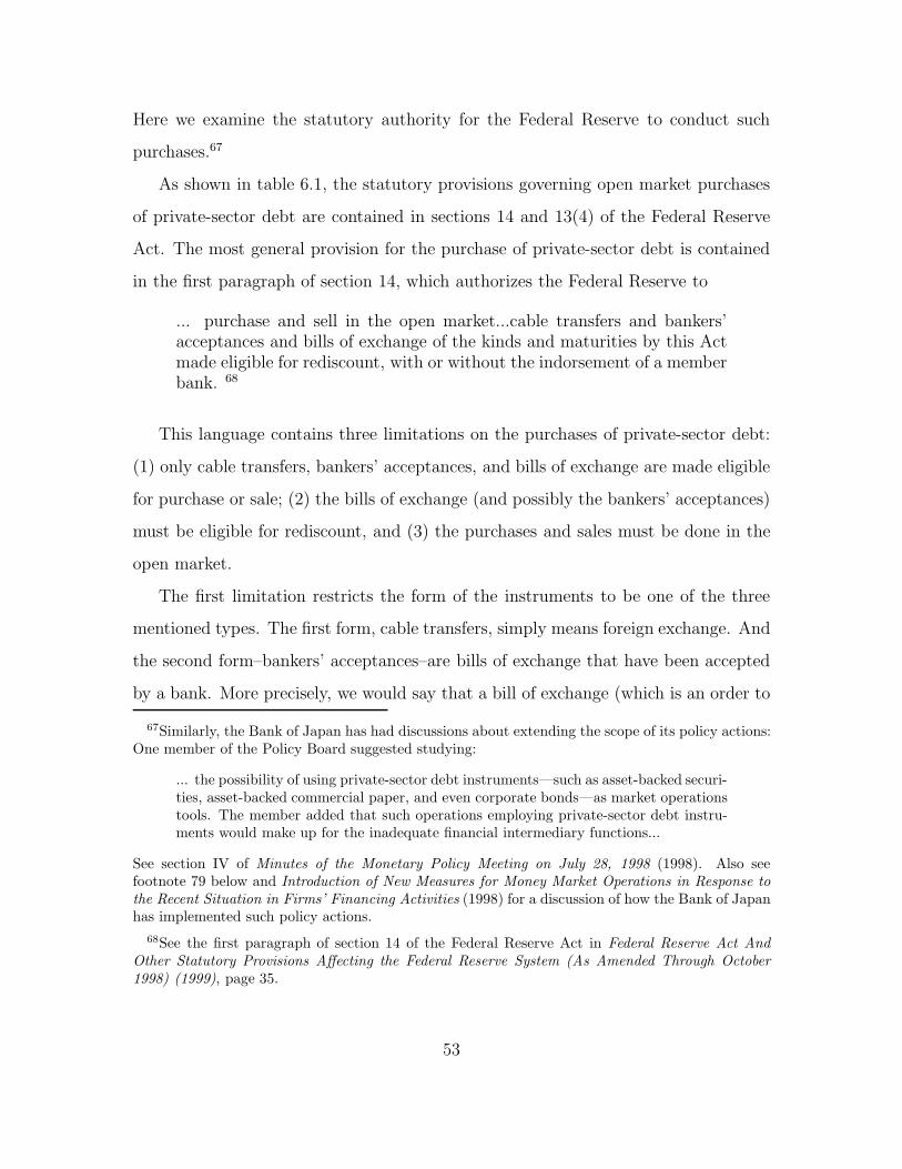
Here we examine the statutory authority for the Federal Reserve to conduct such

purchases.67

As shown in table 6.1, the statutory provisions governing open market purchases

of private-sector debt are contained in sections 14 and 13(4) of the Federal Reserve

Act. The most general provision for the purchase of private-sector debt is contained

in the first paragraph of section 14, which authorizes the Federal Reserve to

... purchase and sell in the open market...cable transfers and bankers’acceptances and bills of exchange of the kinds and maturities by this Actmade eligible for rediscount, with or without the indorsement of a memberbank. 68

This language contains three limitations on the purchases of private-sector debt:

(1) only cable transfers, bankers’ acceptances, and bills of exchange are made eligible

for purchase or sale; (2) the bills of exchange (and possibly the bankers’ acceptances)

must be eligible for rediscount, and (3) the purchases and sales must be done in the

open market.

The first limitation restricts the form of the instruments to be one of the three

mentioned types. The first form, cable transfers, simply means foreign exchange. And

the second form–bankers’ acceptances–are bills of exchange that have been accepted

by a bank. More precisely, we would say that a bill of exchange (which is an order to

67Similarly, the Bank of Japan has had discussions about extending the scope of its policy actions:One member of the Policy Board suggested studying:

... the possibility of using private-sector debt instruments—such as asset-backed securi-ties, asset-backed commercial paper, and even corporate bonds—as market operationstools. The member added that such operations employing private-sector debt instru-ments would make up for the inadequate financial intermediary functions...

See section IV of Minutes of the Monetary Policy Meeting on July 28, 1998 (1998). Also seefootnote 79 below and Introduction of New Measures for Money Market Operations in Response tothe Recent Situation in Firms’ Financing Activities (1998) for a discussion of how the Bank of Japanhas implemented such policy actions.

68See the first paragraph of section 14 of the Federal Reserve Act in Federal Reserve Act AndOther Statutory Provisions Affecting the Federal Reserve System (As Amended Through October1998) (1999), page 35.

53

pay) is transformed into a bankers’ acceptance (which is a promise to pay) upon the

bill of exchange being accepted by a bank.69

The third form–bills of exchange–is a general class of credit instruments, also

generally referred to as “orders to pay”.70 In defining a bill of exchange,

Woelfel states:

A bill of exchange is a three-party instrument in which the first party(drawer) draws an order for the payment of a certain sum on a secondparty (the drawee) for payment to a third party (payee) at a definitefuture time.71

In contrast to bills of exchange, and as discussed in Small and Clouse (2000), debt

instruments such as corporate bonds and mortgages are “promises to pay”: They are

two-party instruments. Thus, this first paragraph of section 14 of the Federal Reserve

Act places a restriction on the Federal Reserve’s open market operations because the

only promises to pay that the paragraph authorizes for purchase or sale are bankers’

acceptances. Because private-sector promises to pay other than bankers’ acceptances

are not made eligible for purchase under the first paragraph of section 14 or under

any other part of the Federal Reserve Act, there is no express authority under which

they may be purchased by the Federal Reserve. Thus there is no express authority

for the Federal Reserve to purchase such promises to pay as corporate bonds, bank

loans, mortgages and credit-card receivables, for example.72 Nor is there any express

authorization for the Federal Reserve to purchase equities.

69See Chandler (1971), pages 158-159.70See section 3.3 in Small and Clouse (2000).71See Woelfel (1994), page 135.72Willis and Steiner (1926) note:

It should be observed that the Act as finally passed excludes the promissory note,the former leading American credit instrument, from open market purchase by reservebanks. In large part this was due to the feeling that the note, not related to a spe-cific transaction nor necessarily bearing an endorsement, could be identified only withdifficulty and hence involved too many hazards.

54

The second limitation is that the bills of exchange must be “of the kinds and

maturities ... eligible for discount.”73 In normal circumstances, the restriction that

the bills of exchange must be eligible for discount would significantly limit the types

of bills of exchange that could be purchased. Purchases would be limited to those

specific types that can be discounted under sections 13(4), 13(6) or 13A of the Federal

Reserve Act (see table 7.1 below) or to those that meet the criteria of section 13(2),

which authorizes the discounting of:

... bills of exchange arising out of actual commercial transactions; thatis, ... bills of exchange issued or drawn for agricultural, industrial, orcommercial purposes ... but such definition shall not include ... billscovering merely investments or issued or drawn for the purpose of carryingor trading in stocks, bonds, or other investment securities, except bondsand notes of the government of the United States.

Thus, in normal circumstances, “eligible for discount” would imply that the bills of

exchange that the Federal Reserve could purchase would have to meet this “real bills”

restriction applicable to discounts under section 13(2) or would have to be the specific

types of bills of exchange eligible for discount under sections 13(4), 13(6), or 13A,

which also seem tied to “real bills” considerations.74

However, if the Board of Governors of the Federal Reserve System found that

there were “unusual and exigent circumstances” and at least five governors voted to

73From the text of the first paragraph of section 14, it is not clear whether this phrase restrictsboth bankers’ acceptances and bills of exchange or only the latter—although the Federal Reserve’sinterpretation appears to have been that it modifies only the latter, as we shall assume henceforth.See Small and Clouse (2000) for a further discussion of this issue.

74Hackley (1973) describes the “real bills” doctrine as: “ ... the Board expounded the principlethat all paper offered for discount should be essentially self-liquidating; in other words, that it ‘shouldrepresent in every case some distinct step in the production or distribution process—the progressionof goods from producer to consumer.’

It was not long before this philosophy—the real-bills doctrine—underwent drastic erosion.” Em-phasis added. (See page 191).

Also see West (1977), chapter 7, for a discussion of the real bills doctrine as providing the theo-retical background for the Federal Reserve Act.

When using “real bills ” in characterizing aspects of the Federal Reserve Act, we will be using itto include agricultural paper, and therefore applying it to paper issued for “agricultural, industrial,or commercial purpose” as per section 13(2) of the Federal Reserve Act.

55

authorize lending under 13(3), the Federal Reserve could discount for IPCs

notes, drafts and bills of exchange ... indorsed or otherwise secured to thesatisfaction of the Federal Reserve bank...” (emphasis added).

If these conditions were met, the bills of exchange eligible for purchase might be

expanded from those meeting the “real bills” criteria to those that are “... secured to

the satisfaction of the Federal Reserve bank.” However, this latter restriction would

seem to limit the ability of the Federal Reserve to purchase assets with considerable

credit-risk premiums.75 Additionally, section 13(3) authorizes discounts only to IPCs

“unable to secure adequate credit accommodations from other banking institutions”.

A third limitation that follows from the first paragraph of section 14 of the Federal

Reserve Act is that the purchases must be conducted in an “open market.” If the

Federal Reserve wanted to purchase large quantities of bankers’ acceptances or bills

of exchange, the “open market” restriction currently could pose a problem because

existing markets for these obligations are not very deep and therefore large “open

market” purchases might not be feasible. In particular, the volume of bankers’ ac-

ceptances in recent years has dwindled to about $25 billion outstanding on average

(at the end of 1996).76 Therefore, the scope for purchasing them is quite limited.77

In a period of economic weakness and financial strains, the attempts of the Federal

Reserve to do what it could to improve economic conditions might lead to market

responses that make these three limitations less binding. First, if the Federal Reserve

made known its desire to purchase bankers’ acceptances and bills of exchange, private-

sector issuance of these instruments might well expand, making the “open market”

75The Board has not had occasion to interpret the section 14 language on bills of exchange in lightof the current language of section 13(3) (as amended in 1991), and thus the implications of section13(3) for purchases under section 14 are open to interpretation. See Small and Clouse (2000) for afurther discussion of this issue, and see section 7.2 below for a discussion of lending under section13(3).

76Source: Federal Reserve Bulletin, Table A22, October, 1998.77The scope would be even more limited if the discount restriction of the first paragraph of section

14 also applies to bankers’ acceptances. See footnote 73.

56

restriction less binding. Second, firms and households might be able to restructure

their financing arrangements so their credit instruments meet the criteria for instru-

ments the Federal Reserve can purchase. And third, even though the proceeds of

such instruments need to meet the “real bills” criteria in usual circumstances, credit

is fungible. Funding secured for “real bills” purposes could free up other funds that

could be used to finance activities other than “real bills” activities.

While purchases of eligible private-sector credit instruments may be a way in

which the Federal Reserve could provide stimulus to aggregate demand, a program

of such purchases has potential problems of its own. By deciding which securities it

was willing to purchase at which prices, the Federal Reserve would be placing itself

in the business of evaluating credit risk. And by doing so, it would be affecting

the allocation of credit across firms and households. The Federal Reserve does not

possess any comparative advantage relative to the private market in doing such credit

evaluations, and credit-risk evaluations and credit allocations could well suffer as a

consequence.

Table 6.2 provides a summary of the private-sector assets that the Federal may

and may not purchase.

57

Table 6.2

Private-Sector Assets Eligible and Ineligiblefor Purchase by the Federal Reserve

1. There is No Express Authority for the Federal Reserve to Purchase:

Corporate BondsCommercial PaperMortgagesEquityLand (Other that Federal Reserve premises)

2. The Federal Reserve May PurchaseGold*Foreign ExchangeBankers’ AcceptancesBills of Exchange

Subject to:

Restriction 1.Purchases of foreign exchange, bankers’ acceptances, and bills ofexchange are to be in the open market.

Restriction 2.In usual circumstances

The bills of exchange must meet the “real bills” doctrine but,it seems, bankers’ acceptances do not.

In “unusual and exigent” circumstancesThe types of bills of exchange that are eligible to be purchasedare open to interpretation.

* Subject to the Gold Reserve Act of 1934.

58

7 Lending by the Federal Reserve

The Federal Reserve’s authority to extend loans is a potentially powerful tool with

which it can stimulate aggregate demand. Loans to depository institutions can help

spur credit extensions to households and firms. If depository institutions are unwilling

or unable to lend to firms and households, direct loans by the Federal Reserve to firms

and households could provide the financing needed for economic recovery–although

such lending is subject to the restrictions discussed below.

7.1 Lending to Depository Institutions

As shown in table 7.1, lending to depositories is authorized under several sections

of the Federal Reserve Act: Advances are authorized under sections 10B, 13(8) and

13(13), while discounts are authorized under sections 13(2), 13(3), 13(4), 13(6) and

13A.78 In recent decades, the Federal Reserve has extended credit to depositories only

through advances (under sections 10B and 13(8)) and has not made any discounts.

The broadest and most flexible authority under which the Federal Reserve can

extend loans to depositories is Section 10B, under which the restriction on collat-

eral is only that the Reserve Bank making the advance deems the collateral to be

“satisfactory”. The collateral can be promissory notes, such as corporate bonds and

commercial paper—instruments that cannot be purchased by the Federal Reserve.

Currently, Reserve Banks accept as collateral various types of promissory notes of ac-

ceptable quality including state and local government securities, mortgages covering

one- to four-family residences, credit-card receivables, other customer notes, commer-

cial mortgages, and business loans. Apparently, even equity shares would be legally

acceptable as collateral if a Reserve Bank found them to be acceptable as collateral.

78The differences between discounts and advances are discussed briefly below and in more detailin Section 2.1 of Small and Clouse (2000).

59

Table 7.1Credit Instruments Used in Discounts or Advances

Borrower Credit Instrument

Depositories10B Advances* Depository’s time and demand notes secured “to the

satisfaction of [the] Reserve Bank.” * *

13(8) Advances Depository’s promissory note secured by U.S Treasury,U.S.-guaranteed, U.S. agency, or U.S. agency-guaranteedsecurities, or by credit instruments eligible for discount or purchase.

13(2) Discounts * * * Notes, drafts and bills of exchange meeting “real bills” criteria.

13(4) Discounts * * * Bills of exchange payable on sight or demand which grow outof the shipment of agricultural goods.

13(6) Discounts * * * Acceptances which grow out of the shipment of goods(section 13(7)) or for the purpose of furnishing dollarexchange as required by the usages of trade (section 13(12)).

13A Discounts * * * Notes, drafts, and bills of exchange secured byagricultural paper.

IPCs * * * *13(13) Advances IPC’s promissory notes secured by U.S. Treasury,

U.S. Agency or U.S. agency-guaranteed obligations.

13(3) Discounts Notes, drafts, and bills of exchange endorsed or otherwisesecured to the satisfaction of the Reserve Bank, in “unusual andexigent circumstances”, and provided the IPC cannot secureadequate credit elsewhere or is in a class for which thisdetermination has been made.

Notes: All advances and the financial instruments used as collateral in all discounts except section 13(discounts are subject to maturity limitations. Section 13(14) authorizes discounts andadvances to branches and agencies of foreign branches, subject to limitations.*Section 10A provides for advances to groups of member banks.* * Advances to undercapitalized and critically undercapitalized institutions are subjectto limitations listed in section 10B.* * * Must be endorsed by a depository institution.* * * * Depository institutions are corporations and thus qualify for lending authorized for IPCs.

60

Even though the Federal Reserve can extend credit to depositories through ad-

vances secured by a wide array of instruments, there may be limitations regarding

the extent to which the Federal Reserve can take onto its balance sheet the credit

risk of a private-sector security pledged as collateral–whether the security is pledged

as part of an advance or a discount. With an advance, the loan is extended on the

basis of a promissory note issued by the depository. During the course of the ad-

vance, should the ability of the depository to repay the advance come under question

(for example, because the collateral is in default) the Federal Reserve would look to

the depository first for repayment: The credit risk of the collateral therefore remains

with the depository.79 In a discount, the depository does not issue its own note to the

Federal Reserve, but the depository must endorse the security that is discounted (as

indicated by the triple asterisks in table 7.1). Again, the credit risk of the underlying

collateral stays with the depository institution, and the only risk the Federal Reserve

takes onto its balance sheet is the risk that the depository will default.80

79In a similar vein, the Bank of Japan recently has undertaken repurchase agreements in com-mercial paper but has acted to protect its balance sheet from the credit risk of the issuer of thecommercial paper:

The Bank recommends commercial paper (CP) operations (purchase of CP with resaleagreements) in order to ensure smooth market operations.CP will be purchased from financial institutions, securities companies, and tanshi com-panies (money market dealers) which hold accounts with the Bank. The CP is to beendorsed by the seller, and to have a maturity of 3 months or less from the day of theBank’s purchase. Purchase is to be made under competitive bidding, and the periodof the purchase is to be 3 months or less. (See Quarterly Bulletin (1996), page 100.)

In September of 1998, the Bank of Japan held, through repurchase agreements, about 35 percent ofthe outstanding stock of commercial paper in Japan. See Table VII in Economic Statistics Monthly(See various dates).

80Discounts under sections 13(2), 13(4) or 13A for a bank require a “waiver of demand, notice andprotest by such bank as to its own endorsement exclusively”, which is discussed by Hackley (1973)(pp. 22). The effect of this waiver is to make the endorsing bank primarily liable because the ReserveBank would not have to demand payment by the issuer of the discounted paper before proceedingagainst the bank. To further limit its credit-risk exposure, the Federal Reserve presumably wouldalso take a “haircut” on the discount by extending funds that are significantly less than the value ofthe discounted instrument. Additionally, the Federal Deposit Insurance Corporation Improvement

61

To the extent the credit risk of the collateral remains with the depository, lend-

ing to depositories may do very little to lower the credit-risk premiums charged by

depositories in making new loans to private-sector borrowers. Credit risk premiums

could be a major factor holding down credit expansion and economic recovery should

nominal rates on Treasury bills be at or near zero and should the economy be weak.

In private-sector markets, credit risk can be managed through the use of credit-

risk options. And, in some circumstances, the Federal Reserve’s incidental powers

clause is consistent with the Federal Reserve using options.81 However, the view that

the Federal Reserve could not accept the credit risk of the collateral used in discount

window loans may leave little scope for the Federal Reserve to write credit-risk options

in order to take that credit risk off the balance sheets of depositories and onto its

balance sheet.

But even if Federal Reserve loans to depositories leave credit-risk premiums un-

changed, such loans may provide some liquidity for the financial instruments used

as collateral—helping to lowering private-sector interest rates by reducing implicit

liquidity premiums.

7.2 Lending to Individuals, Partnerships, and Corporations

Although the Federal Reserve currently does not make loans to individuals, partner-

ships, and corporations (IPCs), the Federal Reserve has the authorization to bypass

depositories and make such loans under sections 13(3) and 13(13) of the Federal Re-

serve Act—as shown in table 7.1. However, lending under these authorities is subject

to very stringent criteria in law and regulation, and such lending has not taken place

since the Great Depression. For example, advances, under section 13(13), are limited

Act of 1991 (FDICIA), through its “prompt corrective action” provisions has imposed restrictionson depository institutions in weak capital condition. Among those restrictions are limitations onaccess to the Federal Reserve’s discount window.

81See footnote 46 for a discussion of the Federal Reserve’s recent use of options, and see Section 4of Small and Clouse (2000) for a discussion of the Federal Reserve’s authority to engage in options.

62

to those

secured by direct obligations of the United States or by any obligationwhich is a direct obligation of, or fully guaranteed as to principal andinterest by, an agency of the United States.

Because IPCs with such collateral could easily sell it in the open market, section 13(13)

advances may not have much effect (unless done at subsidized rates) in stimulating

aggregate demand.

In contrast, private-sector instruments may lack the liquidity of Treasury debt

and, therefore, Federal Reserve loans that use them as collateral may provide liquidity

and help stimulate the economy. Also, in a “credit crunch”, such direct loans would

circumvent depository institutions and the “non-price” terms of credit imposed by

them. Hence, we shall focus on section 13(3) discounts of:

notes, drafts, and bills of exchange when such notes, drafts, and billsof exchange are indorsed or otherwise secured to the satisfaction of theFederal Reserve bank: ...

Because notes, drafts, and bills of exchange include most forms of written credit

instruments, section 13(3) provides virtually no restrictions on the form a credit

instrument must take in order to be eligible for discount.82 And by merely requiring

that the discount be “secured to the satisfaction of the Federal Reserve bank ...”,

there is no restriction on the use of funds (such as for “real bills” purposes) for which

the discounted security was originally issued.

However, in making section 13(3) loans directly to IPCs, the Federal Reserve must

impose standards that are much more stringent in comparison to those used in lending

to a depository. Such lending to IPCs is authorized only in “unusual and exigent

circumstances.” In particular, the statute requires that a loan can be extended only

to IPCs for which credit is not available from other banking institutions.83 Activation

82The distinctions between notes, drafts, and bills of exchange are discussed in detail in Small andClouse (2000).

83The Federal Reserve’s Regulation A (Section 201.3(d): Emergency credit for others) specifiesthat advances to IPCs would be contemplated only in situations in which failure to advance creditwould adversely affect the economy.

63

of this authority requires the affirmative vote of five of the seven governors of the

Federal Reserve Board.

Section 13(3) further requires that the collateral be “indorsed or otherwise secured

to the satisfaction of the Federal Reserve bank ...” As interpreted by Hackley (1973):

... it seems clear that it was the intent of Congress that loans shouldbe made only to credit-worthy borrowers; in other words, the ReserveBank should be satisfied that a loan made under this authority would berepaid in due course, either by the borrower or by resort to security or theendorsement of a third party.84

If binding, this restriction could seriously curtail the effectiveness of such loans in

stimulating aggregate demand in an environment of elevated credit risk and risk

aversion.

But even if the Federal Reserve were able to accept private-sector credit risk onto

its balance sheet, any social benefits to the Federal Reserve lending directly to the

private sector would need to be balanced against the potentially serious drawbacks

associated with placing the Federal Reserve squarely in the process allocating credit

within the private sector. The information available to the Federal Reserve about

nonbank credit would in many cases be inadequate to reliably assess credit risks–

and there is little reason to believe the Federal Reserve could assess credit risks more

accurately than do private intermediaries. Problems with adverse-selection could lead

to the Federal Reserve lending to precisely those credit risks that it most severely

underestimates. After the credit is extended, the Federal Reserve may not be well

situated to monitor the ongoing activities of the recipients of the funds to ensure

the activities are consistent with the terms of the contract. Some of these problems

might be addressed through the Federal Reserve using credit-ratings from private

sector firms.

Moreover, such programs could develop important political constituencies that

might make the programs difficult to dismantle once the immediate aim of policy—

84Hackley (1973), page 129.

64

namely providing a short-run economic stimulus—had been achieved.

65

8 Wealth Creation

In ordinary circumstances, monetary policy exerts its stimulative impact in part

through increasing the financial wealth of the public—such as producing capital gains

in bond and equity markets. If, at the zero bound, the Federal Reserve had already

taken what actions it could to raise bond and equity prices, it might look to other

tools it has to increase the public’s wealth. One tool commonly attributed to the Fed-

eral Reserve, at least in theory if not by the Federal Reserve Act, is that of conducting

“money rains.”

8.1 Money Rains

Money rains are a clean way to study theoretically the effects of increases in the supply

of money. In practice, it seems a bit difficult to envision how the Federal Reserve could

literally implement a money rain—that is give money away either through directly

disbursing currency to the public or by disbursing it through the banking system.

The political difficulties that are likely to arise from the Federal Reserve determining

the distribution of this new wealth would be daunting.

Even if the Federal Reserve were to find a way to physically conduct a money rain,

the Federal Reserve Act does not appear to provide authorization for such activities.

Under section 7 of the Federal Reserve Act,

After all necessary expenses of a Federal reserve bank have been paid orprovided for, the stockholders of the bank shall be entitled to receive anannual dividend of 6 percent on paid-in capital.

That portion of net earnings of each Federal reserve bank which remainsafter dividend claims ... have been fully met shall be deposited in thesurplus fund of the bank.

Thus, any transfers to the public must either be claimed to be “expenses” or be

transfers from the surplus fund.85

85The Federal Reserve currently remits to the U.S. Treasury all net earnings after providing for

66

But Section 7 of the Federal Reserve Act only provides for disposition of surplus

in the event of dissolution or liquidation of the Federal Reserve Banks. A direct

transfer of funds from the surplus account for any other reason—and to the public

in particular— would appear to be beyond the authority of the Reserve Banks. Ap-

parently, then, a money rain would have to be declared an “expense” of the Federal

Reserve. The legal foundation for doing so seems highly questionable.

A second way to distribute newly created money would be to use it to finance a

federal tax cut. A money-financed tax cut could be brought about by the Treasury

financing a tax cut by issuing debt, and the Federal Reserve purchasing that debt. If

the stimulative effects of such open market purchases have already been exhausted by

the Federal Reserve in its attempts to stimulate the economy, the total effect would

come from the fiscal stimulus. Of course, if the fiscal stimulus were large enough

to raise the nominal interest rate above zero, then standard open market operations

would regain their stimulative impact.

These are only two of many possible ways a central bank could attempt to increase

private-sector wealth and thereby stimulate aggregate demand. Putting possible legal

limitations aside, wealth could also be created by purchasing assets at above market

prices or by extending loans at subsidized interest rates. Because these policies de-

liberately create budget deficits, they would seem to be more the province of fiscal

authorities. A consideration of the such attempts to increase private sector wealth is

outside the scope of this paper.

dividends and the amount necessary to equate surplus with paid-in capital. These payments areclassified as interest on Federal Reserve notes and as expenses of the Federal Reserve, and not astransfers from the surplus fund. The authority of the Board of Governors to determine that theFederal Reserve Banks will pay interest on Federal Reserve notes to the U.S. Treasury is granted insection 16(4) of the Federal Reserve Act.

67

9 Conclusion

In an environment of low inflation, the Federal Reserve faces the risk that it may

not have provided enough monetary stimulus even when it has pushed the short-term

nominal interest rate to its lower bound of zero. Whether monetary policy can provide

further stimulus depends on whether monetary policy can affect aggregate demand

through channels other than short-term interest rates and with tools other than open

market operations in Treasury bills.

This paper has examined the alternative policy channels and tools that are avail-

able to the Federal Reserve in theory, and has noted the practical limitations imposed

by the Federal Reserve Act. To affect aggregate demand, the tools the Federal Re-

serve has at its disposal include open market purchases of Treasury bills, Treasury

bonds and private-sector credit instruments (at least those that may be purchased

by the Federal Reserve); unsterilized and sterilized intervention in foreign exchange;

lending through the discount window; and, in some circumstances, the use of options.

When the Treasury bill rate is at zero, further open market purchases of Treasury

bills may yet stimulate aggregate demand even though they do not lower the Treasury

bill rate. An increase in the monetary base, brought about by the purchase of Treasury

bills or of any other asset, possibly could affect aggregate demand by increasing

liquidity; affecting the expected future paths of short-term interest rates, inflation,

and asset prices; or perhaps by spurring lending through credit-channel effects.

When the nominal Treasury bill rate is at zero, the Federal Reserve could attempt

to provide a stimulus to aggregate demand through effects in addition to those from

increases in the monetary base. The Federal Reserve could purchase assets other than

Treasury bills, such as U.S. Treasury bonds or foreign government debt. Even if these

assets are perfect substitutes for U.S. Treasury bills, purchases of them could have

a stronger stimulative impact than purchases of Treasury bills because of “signalling

effects.” In this case, the Federal Reserve balance sheet would benefit from bond

68

prices that are higher than those that would result if it kept short-term interest rates

low. A similar effect is present if the Federal Reserve were to write options in an

attempt to communicate its desired path for the Treasury bill rate.

Absent signalling effects, whether open market operations will have any effects on

aggregate demand depends on the extent to which the assets purchased are imperfect

substitutes for the monetary base and Treasury bills, which are virtually perfect

substitutes at the zero bound. If the assets purchased are imperfect substitutes for

the monetary base and Treasury bills, their interest rates and prices can be affected

by relative supplies. At the zero bound, government bonds and foreign-currency

bills are probably nearly perfect substitutes for the monetary base and Treasury bills

for small- and medium-sized changes in relative supplies. However, very large open

market purchases of government bonds and foreign government debt might well lower

the government bond rate and cause the home currency to depreciate, respectively,

but almost nothing is known about the likely size of these effects.

With extra stimulus possible through the purchase of assets that are imperfect

substitutes for Treasury bills, the purchase of private-sector assets would seem par-

ticularly attractive. Such assets contain credit-risk premiums, and therefore would

not be perfect substitutes for Treasury debt. However, there is no explicit provision

in the Federal Reserve Act under which the Federal Reserve can purchase equities or

private-sector promissory notes such as corporate bonds. And for any long-term debt

that the Federal Reserve may purchase, the zero bound could become a hindrance to

sufficiently stimulating aggregate demand because deflation could keep real long-term

rates elevated. However, the exchange value of the dollar does not face a similar lower

bound.

But with discount window loans—whether in the form of advances or discounts—

the Federal Reserve can accept as collateral (and therefore make “liquid” for a deposi-

tory) a wide variety of assets that the Federal Reserve cannot purchase. A potentially

serious limitation on such loans is that it has apparently been the intent of Congress

69

that the Federal Reserve not take onto its balance sheet the credit-risk of the col-

lateral: The Federal Reserve could turn to the depository for full payment of the

loan.

The Federal Reserve can bypass depositories and lend directly to individuals,

partnerships, and corporations (IPCs). However, the Federal Reserve must find there

to be “unusual and exigent” conditions and the IPC receiving the loan must be unable

to secure credit from other banking institutions. It seems the intent of Congress was

that the Federal Reserve should make such loans only to credit-worthy IPCs.

With the Federal Reserve not taking credit risk onto its balance sheet, private-

sector loan markets would still incorporate all credit risk into any new loans to house-

holds and businesses—preventing any decline in credit-spreads, which may be elevated

should the economy be at the zero bound and should the economy be weak. Nonethe-

less, loans by the Federal Reserve to depositories and to IPCs could provide some liq-

uidity for the credit instruments used as collateral and thereby could lower liquidity

premiums.

Even if these restrictions on accepting private-sector credit risk were surmounted,

or relaxed by an act of Congress, direct involvement by the Federal Reserve in the

credit allocation process would raise a number of difficult issues because the Fed-

eral Reserve would have to assess credit risk, choose among private borrowers, and

monitor repayment prospects while loans were outstanding. How well or poorly the

Federal Reserve performed these functions would affect the allocation of credit across

individuals and sectors in the economy.

In sum, despite the limitations imposed by the Federal Reserve Act, the Federal

Reserve has a wide range of policy actions it can undertake to stimulate aggregate

demand should the nominal Treasury bill rate be at zero. But these tools have their

limitations, and there is considerable uncertainty regarding their likely effectiveness.

Phelps (1972) noted this uncertainty and concluded that long-run inflation should be

kept above zero:

70

... the costs incurred and the errors made in the attempt to stabilize theeconomy will be much greater at low rates of interest than at high rates.At low rates of inflation the trials of the stabilizers are made harder andtheir tools are made blunter and less reliable. In a world of uncertainty, apolicy of moderately high inflation in order to contain liquidity somewherebelow the otherwise ideal level imposes a cost which can be viewed as thepremium charged for (limited!) insurance against economic instability...Some positive amount of insurance would seem to be definitely worthbuying. (See page 210.)

However, the mere existence of some, even considerable, uncertainty should not be

seen as a convincing reason why inflation should be kept elevated permanently. If the

Federal Reserve were to start to use tools heretofore unused, markets might respond

in ways that make those tools more effective: For example, the private sector could

restructure their financing arrangements so their new credit instruments are of the

type that the Federal Reserve can purchase. But absent endogenous changes in finan-

cial markets, changes in the Federal Reserve Act, and reductions in the uncertainty

about the effectiveness of alternative monetary policy tools at the zero bound, the

zero bound potentially could be an important factor in limiting how low the Federal

Reserve should set its target or lower bound for long-run inflation.

But, if the economy is mired in a zero-bound recession, it may well be worth using

the monetary policy actions considered in this paper even though they may have

uncertain effects. The case for undertaking such policy actions is buttressed if they

are thought to have no adverse effects. Some potential downside risks of such policies

have been discussed in the context of recent experience in Japan by Okina (1999),

McKinnon, Meltzer and Okina (1999), and Yamaguchi (1999).

If the economy is in a zero-bound recession, the particular monetary policy tool or

mix of policy tools that will be most effective may depend on the particular cause of

the recession. For example, a central bank may engage in unsterilized interventions

to test the effectiveness of these interventions in stimulating aggregate demand. But

if the cause of the recession were a credit crunch, then tools more directly focused on

the banking sector might be given a larger relative weight in the mix of policy actions

71

designed to bring the economy up to full employment—especially if the tools directed

toward the banking sector can be employed in a manner that provides improved

incentives for the banking sector going forward. Indeed, the successful implementation

of such a tool may make other monetary policy tools that stimulate overall aggregate

demand more effective.

72

References

Baumol, William J., “The Transactions Demand for Cash: An Inventory TheoreticApproach,” Quarterly Journal of Economics, November 1952, 66, 546–56.

Bernanke, Ben and Mark Gertler, “Inside the Black Box: The Credit Channelof Monetary Policy Transmission,” Journal of Economic Perspectives, 1995, 9(4), 27–48.

Black, Fischer, “The Pricing of Commodity Contracts,” Journal of Financial Eco-nomics, January/March 1976, 3, 167–79.

Brayton, F., E. Mauskopf, D. Reifschneider, P. Tinsley, and J. Williams,“The Role of Expectations in the FRB/US Macroeconomic Model,” Fed-eral Reserve Bulletin, April 1997, 83, 227–245. Website address:http://www.bog.frb.fed.us/pubs/bulletin.

Brayton, Flint and Peter Tinsley, “A Guide to FRB/US: A MacroeconomicModel of the United States,” Finance and Economics Discussion Series, 1996,1996-42. Website address: http://www.bog.frb.fed.us/pubs/feds.

Bryant, Ralph C., Gerald Holthman, and Peter Hooper, “Consensus And Di-versity in Model Simulations,” in Ralph C. Bryant, Dale W. Henderson, GeraldHolthman, Peter Hooper, and Stephen A. Symanski, eds., Emprical Macroeco-nomics for Interdependent Economies, Washington DC: The Brookings Institute,1988.

Buiter, Willem H. and Nikolaos Panigirtzoglou, “Liquidity Traps: How toAvoid Them and How to Escape Them,” 1999. The paper is available atwww.econ.cam.ac.uk/faculty/buiter/index.htm.

Cecchetti, Stephen, “The Case of the Negative Nominal Interest Rates: New Es-timates of the Term Structure of Interest Rates during the Great Depression,”Journal of Political Economy, December 1988, 96 (6), 1111–41.

Chandler, Lester V., American Monetary Policy, New York, Evanston, San Fran-cisco, London: Harper and Row, 1971.

Cole, Harold L. and Narayana Kocherlakota, “Zero Nominal Interest Rates:Why They’re Good and How to Get Them,” Quarterly Review, 1998, Spring.Federal Reserve Bank of Minneapolis.

Economic Statistics Monthly, Bank of Japan, See various dates.

Fedenia, M. and T. Grammatikos, “Options Trading and the Bid-Ask Spread ofthe Underlying Stocks,” Journal of Business, July 1992, 65, 335–51.

73

Federal Reserve Board, Banking and Monetary Statistics, Washington DC: FederalReserve Board, 1943.

Federal Reserve Act And Other Statutory Provisions Affecting the Fed-eral Reserve System (As Amended Through October 1998), Washing-ton D.C.: Board of Governors of the Federal Reserve System, 1999. Copiesmay be obtained from Publications Services, Board of Governors of the FederalReserve System, MS-138, Washington D.C., 20551.

Financial Services Institutions: Information for Assessing the Govern-ment’s Potential Financial Exposure, Washington, D.C.: United StatesGeneral Accounting Office, June 1998.

Fischer, Stanley, “Why are Central Banks Prusuing Long-Run Price Stability?,”in “Achieving Price Stability,” Federal Reserve Bank of Kansas City, 1996.

Fleming, Michael J., “The Benchmark U.S. Treasury Market: Recent Performanceand Possible Alternatives,” Federal Reserve Bank of New York Economic PolicyReview, forthcoming 2000.

Fuhrer, Jeffrey and Mark Schneiderman, eds, in Jeffrey Fuhrer and MarkSchneiderman, eds., Monetary Policy in a Low-Inflation Environment, Journalof Money, Credit and Banking, November 2000.

Fuhrer, Jeffrey C. and Brian Madigan, “Monetary Policy When Interest Ratesare Bounded at Zero,” Review of Economics and Statistics, November 1997, 79,573–85.

Goodfriend, Marvin, “Overcoming the Zero Bound on Interest Rate Policy,” Oc-tober 1999. Prepared for the Federal Reserve Confernce ’Monetary Policy in aLow-Inflation Environment,’ Woodstock, VT.

Hackley, Howard H., Lending Function of the Federal Reserve Banks: A History,Washington, D.C.: Board of Governors of the Federal Reserve System, May1973.

Hanes, Christopher, “The Liquidity Trap, the Supply of Reserves and U.S. InterestRates in the 1930s,” July 1999. manuscript, Board of Governors of the FederalReserve System.

Hicks, John, “Mr. Keynes and the ‘Classics’,” Econometrica, April 1937, 5 (2).

Hull, John, Options, Futures, and Other Derivatives, third ed., Upper Saddle River,NJ: Prentice-Hall, 1997.

74

Introduction of New Measures for Money Market Operationsin Response to the Recent Situation in Firms’ Financ-ing Activities, Bank of Japan, November 1998. Website address:http://www.boj.or.jp/en/seisaku/98/sei9811.htm.

Ireland, Peter N., “The Role of Countercyclical Monetary Policy,” Journal of Po-litical Economy, August 1996, 104, 704–723.

Johnson, Karen, David Small, and Ralph Tryon, “Monetary Policy and PriceStability,” July 1999. International Finance Discussion Papers, Board of Gov-ernors of the Federal Reserve System,Washington D.C. (Also forthcoming inProceedings of a Conference on Possiblities and Limitations of Monetary Policy,held on June 10-11, 1999 at the Austrian National Bank in Vienna).

Koziki, Sharon and P.A. Tinsley, “Term Structure Views of Monetary PolicyUnder Alternative Models of Agent Expectations,” July 1999. Forthcoming inthe Journal of Economic Dynamics and Control.

Krugman, Paul, “It’s Baaack! Japan’s Slump and the Return of the LiquidityTrap.,” Brookings Papers on Economic Activity, 1998, 2, 137–205.

, “Japan’s Trap,” June 1998. Also see: Further Notes on Japan’s Liqudity Trap,Website address: http://web.mit.edu/krugman/www.

Lebow, David, “Monetary Policy at Near-Zero Interest Rates,” Working Paper 136,Economic Activity Section, July 1993.

Lowell, Linda, “Mortgage Pass-Through Certificates,” in Frank J. Fabozzi, ed., TheHandbook of Mortgage Backed Securities, Probus Publishing, 1995.

Macauley, Frederick, Some Theoretical Problems Suggested by the Movements ofInterest Rates, Bond Yields and Stock Prices in the United States Since 1856,New York: NBER, 1938.

McKinnon, Ronald, Allan Meltzer, and Kunio Okina, “Monetary Policy Un-der Zero Inflation—A Response to Criticisms and Questions Regarding MonetaryPolicy—Comments and Rejoinder,” July 1999. IMES Discussion Paper Series99-E-28, Institute for Monetary and Economic Studies, Bank of Japan. Availableat www.boj.or.jp/en/ronbun/ronbun.htm.

Meltzer, Allan H., “The Transmission Process,” March 1999. manuscript, CarnegieMellon University and the American Enterprise Institute.

Merton, Robert, “Financial Innovation and the Management and Regulation ofFinancial Institutions,” Journal of Banking and Finance, June 1995, 19, 461–81.

Meulendyke, Ann-Marie, U.S. Monetary Policy and Financial Markets, FederalReserve Bank of New York, 1998.

75

Minutes of the Monetary Policy Meeting on July 28, 1998, Bank of Japan,1998. Website address: http://www.boj.or.jp/en/seisaku/98/pb/g980728.htm.

Mishkin, Frederick S., “The Channels of Monetary Transmission: Lessons forMonetary Policy,” 1996. NBER Working Paper 5464.

Modigliani, Franco and Richard Sutch, “Innovations in Interest Rate Policy,”American Economic Review, May 1966, pp. 178–97.

Monetary Policy and Reserve Requirements Handbook, Washington, D.C.:Federal Reserve Regulatory Service, Board of Governors of the Federal ReserveSystem, 1998.

Mullins, David, “Challenges for Monetary Policy in the Evolving Financial En-vironment,” in I. Kuroda, ed., Towards More Effective Monetary Policy, NewYork: St. Martins Press., 1997, pp. 99–129.

Mussa, Michael, “The Role of Official Intervention,” Group of Thirty OccassionalPapers, no. 6. New York: Group of Thirty, 1981.

Okina, Kunio, “Monetary Policy Under Zero Inflation–A Response to Criticismsand Questions Regarding Monetary Policy,” July 1999. IMES Discussion PaperSeries 99-E-20, Institute for Monetary and Economic Studies, Bank of Japan.Available at www.boj.or.jp/en/ronbun/ronbun.htm.

Orphanides, Athanasions and Volker Wieland, “Efficient Monetary Policy De-sign Near Price Stability,” Finance and Economics Discussion Series, December1999, 1999-67. Website address: http://www.bog.frb.fed.us/pubs/feds.

Orphanides, Athanasios and Volker Wieland, “Price Stability and MonetaryPolicy Effectiveness when Nominal Interest Rates are Bounded at Zero,” Financeand Economics Discussion Series, 1998-35, August 1998. Board of Governors ofthe Federal Reserve System.

Patinkin, Don, “Price flexibility and full employment,” in Harold R. Williams andJohn D. Huffnagle, eds., Macroeconomic Theory: Selected Readings, PrenticeHall, Inc., 1951.

Phelps, Edmund S., Inflation Policy and Unemployment Theory, London: TheMacMillan Press Ltd., 1972.

Quarterly Bulletin, Bank of Japan, February 1996.

Reifschneider, David and John C. Williams, “Three Lessons for MonetaryPolicy in a Low Inflation Era,” September 1999. Working Paper, Board ofGovernors of the Federal Reserve System.

76

Shiller, Robert J., “The Volatility of Long-Term Interest Rates and ExpectationsModels of the Term Structure,” Journal of Political Economy, 1979, 87 (6),1190–1219.

, John Y. Campbell, and Kermit L. Schoenholtz, “Forward Rates andFuture Policy: Interpreting the Term Structure of Interest Rates,” BrookingsPapers on Economic Activity, 1983, 1, 173–224.

Small, David and James Clouse, “The Limits the Federal Reserve Act Places onthe Monetary Policy Actions of the Federal Reserve,” 2000. Board of Governorsof the Federal Reserve System An earlier version of this paper was published inthe Annual Review of Banking Law, 2000, Vol. 19: pp. 553-579.

Stanton, Thomas H., A State of Risk: Will Government-Sponsored Enterprises BeThe Next Finanical Crisis?, Harper-Collins, 1991.

Stigum, Marcia, The Money Market, Homewood, Illinois: Dow Jones-Irwin, 1990.

Summary of Marketable Treasury Inflation-Indexed Securities, 1999. U.S.Treasury website address: www.publicdebt.treas.gov/of/ofinflin.htm.

Svensson, Lars E.O., “How Should Monetary Policy Be Conducted in an Era ofPrice Stability?,” August 1999. Institute for International Economic Studies,Stockholm University.

Taylor, John B., “Discretion Versus Policy Rules in Practice,” Carnegie-RochesterConference Series on Public Policy, 1993, 39, 195–214.

Tetlow, Robert and John C. Williams, “Implementing Price Stability: Bands,Boundaries and Inflation Targeting,” March 1998. Federal Reserve Board staffworking paper.

Tinsley, Peter A., “Short Rate Expectations, Term Premiums, and Central BankUse of Derivatives to Reduce Policy Uncertainty,” February 1999. FRB staffworking paper, Financial and Economics Discussion Series (FEDS) 1999-14.

Tobin, James, “Commercial Banks as Creators of ‘Money’,” in Deane Carson, ed.,Banking and Monetary Studies, Richard Irwin Inc., 1963.

, “Money and Finance in the Macroeconomic Process,” Journal of Money, Creditand Banking, May 1982, 14, 171–203. Noble Lecture.

Turnbull, S. and L. Wakeman, “A Quick Algorithm for Pricing European AverageOptions,” Journal of Financial and Quantitative Analysis, September 1991, 26,377–89.

West, Robert Craig, Banking Reform and the Federal Reserve, 1863-1923, CornellUniversity Press, 1977.

77

Willis, H. Parker and William H. Steiner, Federal Reserve Banking Practice,New York: D. Appleton and Company, 1926.

Woelfel, Charles J., Encyclopedia of Banking and Finance, Chicago, Illinois:Probus Publising Company, 1994.

Wolman, Alexander, “Real Implications of the Zero Bound on Nominal InterestRates,” November 1998. Federal Reserve Bank of Richmond.

World Economic Outlook, International Monetary Fund, October 1999.

WuDunn, Sheryl, “Zen Banking: Japan’s Negative Interest Rates,” New YorkTimes, November 7 1998, p. B1.

Yamaguchi, Yutaka, “Monetary Policy and Structural Policy: A Japanese Perspec-tive,” November 1999. Remarks by Yutaka Yamaguchi, Deputy Governor of theBank of Japan, before Collaque Monetaire International at Banque de France,October 8-9, 1999. Available at www.boj.or.jp/en/press/press f.htm.

Zuckerman, Gregory and Chikako Mogi, “T-Bills’ Yield In Japan Shifts To TheNegative,” Wall Street Journal, November 6 1998, p. C1.

78

Index

Baumol, William, 25Bernanke, Ben, 28, 29Black, Fischer, 38Brayton, Flint, 2Bryant, Ralph, 46Buiter, Willem, 1

Campbell, John, 32Cecchett, 8Cecchetti, Stephen, 10Chandler, Lester, 16Clouse, James, 4, 36, 47, 54, 55, 59, 62,

63Cole, Harold, 25

Fedenia, M., 40Fischer, Stanley, 1Fleming, Michael, 34Fuhrer, Jeffrey, 1

Gertler, Mark, 28, 29Goodfriend, Marvin, 1Grammatikos, T., 40

Hackley, Howard, 4, 55, 61, 64Hanes, Christopher, 34Hicks, John, 10Hooper, Peter, 46Hothman, Gerald, 46Hull, John, 37, 40

Ireland, Peter, 25

JapanMonetary Policy

Bank of Japan: Actions and Dis-cussions, 53, 61, 71

Recommendations, 27Recent Experience, 19–21

Johnson, Karen, 1

Keynes, John Maynard, 10Kocherlakota, Narayana, 25

Krugman, Paul, 25–27

Lebow, David, 4

Macauley, Frederick, 6Madigan, Brian, 1Mauskopf, Eileen, 2Meltzer, Allan, 4, 23, 33Merton, R., 37Meulendyke, Ann Marie, 34Mishkin, Frederick, 22Modigliani, Franco, 33Mogi, Chikako, 21Mullins, David, 40

Operation Twist, 34Options, 28, 35–41, 62Orphanides, Athanasios, 2, 28, 46

Panigirtzoglou, Nikolaos, 1Patinkin, Don, 2Phelps, Edmund, 1, 70

Real Bills Doctrine, 55Reifschneider, David, 1–3Ricardian Equivalence, 23

Schoenholtz, Kermit, 32Shiller, Robert, 32Small, David, 1, 4, 36, 47, 54, 55, 59,

62, 63Stigum, Marcia, 12Summers, Lawrence, 1Sutch, Richard, 33Svensson, Lars, 1

Taylor, John, 2Tetlow, Robert, 1, 2Tinsley, Peter, 2, 35Tobin, James, 4, 23, 24, 33Treasury Inflation-Protected Securities,

31Tryon, Ralph, 1

79

Turnbull, S., 37

Wakeman, L., 37West, Robert Craig, 55Wieland, Volker, 2, 28, 46Williams, John, 1–3Woelfel, Charles, 54Wolman, Alexander, 26, 27WuDunn, Sheryl, 21

Zuckerman, Gregory, 21

80