Monetary Policy Transmission during Financial … Policy Transmission during Financial Crises: An...

Working Paper/Document de travail 2014-21

Monetary Policy Transmission during Financial Crises: An Empirical Analysis

by Tatjana Dahlhaus

2

Bank of Canada Working Paper 2014-21

June 2014

Monetary Policy Transmission during Financial Crises: An Empirical Analysis

by

Tatjana Dahlhaus

International Economic Analysis Department Bank of Canada

Ottawa, Ontario, Canada K1A 0G9 [email protected]

Bank of Canada working papers are theoretical or empirical works-in-progress on subjects in economics and finance. The views expressed in this paper are those of the author.

No responsibility for them should be attributed to the Bank of Canada.

ISSN 1701-9397 © 2014 Bank of Canada

ii

Acknowledgements

I am grateful to Luca Gambetti for his very helpful guidance. I also thank Frank Schorfheide, Fabio Canova, Juan Rubio-Ramirez, Juan Carlos Conesa, Evi Pappa, and Tatevik Sekhposyan as well as seminar participants at the UAB, Bank of Canada, Bank of Mexico, ECB, DIW, Banca d’Italia, and Norway Statistics for helpful comments and suggestions.

iii

Abstract

This paper studies the effects of a monetary policy expansion in the United States during times of high financial stress. The analysis is carried out by introducing a smooth transition factor model where the transition between states (“normal” and high financial stress) depends on a financial conditions index. Employing a quarterly data set over the period 1970Q1 to 2009Q2 containing 108 U.S. macroeconomic and financial time series, I find that a monetary policy shock during periods of high financial stress has stronger and more persistent effects on macroeconomic variables such as output, consumption, and investment than it has during “normal” times. Differences in effects among the regimes seem to originate from non-linearities in the credit channel.

JEL classification: C11, C32, E32, E44, G01 Bank classification: Financial markets; Econometric and statistical methods; Transmission of monetary policy

Résumé

L’auteure étudie les effets d’une politique monétaire expansionniste aux États-Unis en périodes de fortes tensions financières. Pour procéder à son analyse, elle élabore un modèle factoriel à transition lisse dans lequel le passage d’un état à l’autre (d’une situation « normale » à un régime de fortes tensions) dépend d’un indice des conditions financières. À partir de données trimestrielles allant du premier trimestre de 1970 au deuxième trimestre de 2009, soit 108 séries chronologiques de données macroéconomiques et financières américaines, l’auteure observe qu’un choc de politique monétaire a des répercussions plus importantes et persistantes sur des variables macroéconomiques comme la production, la consommation et l’investissement s’il survient en période de fortes tensions plutôt que lorsque la conjoncture est « normale ». L’incidence différente selon le régime (« normal » / fortes tensions) semble attribuable à la non-linéarité du canal du crédit par lequel se transmettent les mesures de politique monétaire.

Classification JEL : C11, C32, E32, E44, G01 Classification de la Banque : Marchés financiers; Méthodes économétriques et statistiques; Transmission de la politique monétaire

Non-technical summary

The U.S. economy has experienced several financial crises in the past 40 years. Financial

conditions have long been understood to play an important role in macroeconomic dynamics

and the recent financial crisis has strengthened interest in exploring the interactions between

monetary policy and financial market imperfections. Policy-makers reduced interest rates

to historical lows in order to support demand and alleviate the financial stress and its

contractionary effects on the economy. Some interesting and natural questions arise: are

the effects on economic activity of conventional monetary policy, i.e., decreasing the federal

funds rate, different during periods of high financial stress from what is usually observed

in good or “normal” times? Have the transmission channels of U.S. monetary policy been

different during the financial crises of the past 40 years?1

This paper aims to shed light on these questions and contributes to the literature in

two ways: first, since the questions at hand demand a non-linear environment, I develop

an empirical model, which allows monetary policy shocks to propagate differently in times

of low and high financial stress; second, I use this model to study the transmission of a

conventional monetary policy shock in the United States during times of low or normal and

high financial stress.

The analysis is of interest because the literature has not yet reached a consensus on

whether and how responses of macroeconomic variables to monetary policy shocks differ

in times of financial stress from what is usually observed in normal times. On the one

hand, it has been argued that monetary policy has not been effective during financial crises.

This view is motivated by the fact that, during the recent financial crisis, credit standards

tightened despite the Federal Reserve decreasing interest rates substantially. On the other

hand, one might argue that monetary policy has been effective and actually more potent

during financial crises, since it not only lowers interest rates on default-free securities, but

also helps to lower credit spreads. This view can be linked to the credit channel of monetary

policy or the so-called financial accelerator. The impact of the financial accelerator is

assumed to be non-linear, meaning that its effects are stronger the lower the financial

conditions of the borrower, i.e., lower net worth and higher cost of credit. Therefore, during

times of high financial stress, firms and households would be more sensitive to any change

1Throughout the paper, I define financial crises as periods of high financial stress.

2

in their cost of credit induced, for example, by a monetary policy shock.

To study the effects of monetary policy during times of high financial stress in the United

States, I employ a data set that contains 108 quarterly series over the period 1970 to 2009.

Estimating the empirical model, I find the following main results: first, a monetary policy

shock has stronger and more persistent effects on macroeconomic variables such as output,

consumption, and investment during financial crises than it has during normal times; second,

differences in effects among the two regimes seem to originate from non-linearities in the

credit channel.

More specifically, I find that a negative monetary policy shock decreases the external

finance premium (EFP) and increases stock prices, i.e., the entrepreneurs’ wealth, in the

financial crises as well as the normal regime. The effects on the EFP and stock prices

are stronger during financial crises. This provides supportive evidence for the existence

of a balance-sheet channel that is more pronounced during times of high financial stress.

Moreover, an expansionary monetary policy shock increases loans during financial crises

while it seems to have no significant effects on loans during times of low financial stress,

indicating the potential existence of a bank-lending channel during periods with severe

disruptions in financial markets. Summing up, a monetary expansion during financial crises

increases loans and asset prices by more than in times of low financial stress, leading to a

higher decrease of the EFP which, in turn, provokes the stronger effects of macroeconomic

variables such as output, investment, consumption, and employment.

3

1 Introduction

The U.S. economy has experienced several financial crises in the past 40 years. Financial

conditions have long been understood to play an important role in macroeconomic dynamics

and the recent financial crisis has strengthened interest in exploring the interactions between

monetary policy and financial market imperfections. Policy-makers reduced interest rates

to historical lows in order to alleviate the financial stress and its contractionary effects on

the economy. Some interesting and natural questions arise: are the effects on economic

activity of conventional monetary policy, i.e., decreasing the federal funds rate, different

during periods of high financial stress from what is usually observed in good or “normal”

times? Have the transmission channels of U.S. monetary policy been different during the

financial crises of the past 40 years?

This paper aims to shed light on these questions and introduces an empirical model

which allows for non-linearities in the dynamic propagation of monetary policy shocks along

financial conditions. In particular, I study the transmission of conventional monetary policy

during times of low (normal) and high financial stress. So far, little empirical work has been

devoted to the investigation of monetary policy transmission during financial crises. Among

the very few papers addressing the issue that transmission of shocks may depend on the

level of financial stress are Davig and Hakkio (2010) and Hubrich and Tetlow (2012), who

both employ a Markov-switching vector autoregression (VAR). Davig and Hakkio (2010)

focus on the effects of financial shocks and find that increases in financial stress have had a

much stronger effect on the real economy when the economy is in a distressed state. Hubrich

and Tetlow (2012) show that macroeconomic dynamics are highly dependent on financial

conditions. Moreover, while not explicitly modelling monetary policy, their counterfactual

experiments suggest that conventional monetary policy is not particularly effective in times

of high financial stress. In this paper, I contribute to the literature in two ways: first, a

conventional monetary policy shock is explicitly identified in the model in order to study its

effects depending on the level of financial stress; second, the analysis not only establishes

the existence of differences in monetary policy transmission during periods of high financial

stress, but exploits where these differences stem from.

The economic profession has not yet reached a consensus on whether and how responses

of macroeconomic variables to monetary policy shocks differ in times of high financial stress

4

from what is usually observed in normal times. On the one hand, it has been argued

that monetary policy has not been effective during financial crises. This view is motivated

by the fact that, during the recent financial crisis of 2008/09, credit standards tightened

and the cost of credit increased further, despite the Federal Reserve reducing interest rates

substantially (see Krugman (2008)). On the other hand, one might argue that monetary

policy has been effective and actually more potent during financial crises because it not only

lowered interest rates on default-free securities, but also helped to lower credit spreads. Since

shocks from the recent financial crisis were unusually large versions of shocks previously

experienced (Stock and Watson (2012)), one might argue that monetary policy was simply

not able to offset these massive contractionary shocks (see Mishkin (2009)).

The latter view can be linked to the credit channel of monetary policy or the so-called

financial accelerator mechanism (see the seminal contributions of Bernanke and Gertler

(1989), Bernanke et al. (1996) and Bernanke et al. (1999)). The key premise of the financial

accelerator is the inverse relationship between the premium that borrowers have to pay

when they ask for external credit in the banking system (the so-called external finance

premium (EFP)) and the financial condition of the borrower. The impact of the financial

accelerator is assumed to be non-linear, i.e., its effects are stronger the lower the financial

fundamentals such as the net worth of firms or the higher the cost of credit. During normal

times, when financial stress is low, firms and households are less sensitive to changes in their

cost of credit, whereas during times of high financial stress or crises, firms and households

are more sensitive to any change in their cost of credit. Therefore, changes in the net worth

induced by, for example, monetary policy may yield large changes in the cost of credit for

low-net-worth borrowers (borrowers during financial crises), but should not much affect the

cost of credit for borrowers with wide internal finance (borrowers in normal times).2

The possibility of a non-linear credit channel has been noted in the literature by, for

example, Bernanke and Gertler (1989), Gertler and Gilchrist (1994), and Bernanke et al.

(1999). Bernanke et al. (1999), using a two-sector model with the financial accelerator, find

that firms with relatively poor access to external credit markets respond more strongly to an

expansionary monetary policy shock than do firms with better access to credit. Moreover,

Gertler and Gilchrist (1994) provide empirical evidence that the performance of small firms

2Note that, during financial crises, when asset prices are low firms are likely to be liquidity constrainedand in need of external financing.

5

is more sensitive to interest rate changes the weaker the balance sheets of the firms, sug-

gesting that financial accelerator effects should be stronger the higher the financial stress.

Finally, Ravn (2014) introduces a model in which the strength of the financial accelerator is

non-linear. The asymmetric financial accelerator is modelled by assuming different values

of the elasticity of the EFP with respect to the net worth of firms. This implies that when

the entrepreneurs’ wealth is already low, such as during financial crises, the EFP reacts

more strongly to small changes in net worth.

Since the questions at hand demand a non-linear environment, I introduce the smooth

transition factor model (STFM), which is a regime-dependent factor model where the tran-

sition between regimes (of normal and high financial stress) is smooth. In contrast to

estimating a model for each regime separately, a smooth transition model makes use of

more information by exploiting variations in the probability of being in a particular regime

so that estimation for each regime is based on a larger set of observations. Moreover, since I

am especially interested in exploring where differences in effects of a monetary policy shock

stem from, the STFM allows me to obtain conditional regime-dependent responses from

a broad set of macroeconomic and financial variables. As a conditioning factor, I use a

financial conditions index summarizing information from financial market variables. The

STFM is estimated using Bayesian Markov chain Monte Carlo (MCMC) methods, i.e., a

Metropolis-within-Gibbs sampler.

Estimating the model using 108 macroeconomic and financial variables over the period

1970Q1 to 2009Q2, I find the following main results:

1. A monetary policy shock has stronger and more persistent effects on macroeconomic

variables such as output, consumption, and investment during financial crises than

during normal times.

2. Differences in effects among the regimes seem to originate from non-linearities in the

credit channel.

More specifically, I find that a monetary expansion decreases the EFP and increases

stock prices, i.e., entrepreneurs’ wealth, in the financial crises as well as the normal regime.

The effects on the EFP and stock prices are stronger during financial crises. This provides

supportive evidence for the existence of a balance-sheet channel that is more pronounced

6

during times of high financial stress. Moreover, an expansionary monetary policy shock

increases loans during financial crises while it seems to have no significant effects on loans

during times of low financial stress, indicating the potential existence of a bank-lending

channel during periods with severe disruptions in financial markets. Summing up, a mone-

tary expansion during financial crises increases loans and asset prices by more than in times

of low financial stress, leading to a higher decrease of the EFP which, in turn, provokes the

stronger effects of macroeconomic variables such as output, investment, and consumption.

The remainder of this paper is organized as follows: Section 2 introduces the STFM;

the Metropolis-within-Gibbs sampler used to estimate the model is described in Section 3;

Section 4 reports the empirical results of the analysis; Section 5 concludes.

2 The Smooth Transition Factor Model

This section introduces the smooth transition factor model (STFM). The model is based

on the dynamic factor model (see, e.g., Forni et al. (2009)), into which I introduce a non-

linear relation among the common factors. To allow for responses being different across

normal times and times of high financial stress, i.e., financial crises, I employ a smooth

transition vector autoregression (STVAR) for the factors (see, for example, Weise (1999)

and Auerbach and Gorodnichenko (2012)). The STVAR is a multivariate extension of the

smooth transition autoregressive models developed in Granger and Terasvirta (1993).

The key advantage of estimating an STVAR for the factors rather than estimating

structural vector autoregressions for each regime separately is that with the latter I may

have relatively few observations in a regime, especially for episodes of high financial stress.

In contrast, by specifying the factors as an STVAR, the dynamics of the common factors

may be determined by both regimes, with one regime having more impact in some times

and the other regime having more impact in other times. Therefore, the model makes use of

more information by exploiting variations in the probability of being in a particular regime,

so that estimation for each regime is based on a larger set of observations.

Let xt = (x1t, x2t, ..., xNt)′ be an N -dimensional vector of macroeconomic variables at

7

time t, t = 1, ..., T . xt has the following factor model representation:

xt = χt + et (1)

= Λ′ft + et,

where ft is an r × 1 vector of unobserved “common” or “static” factors and Λ is an r ×N

matrix of factor loadings associated with ft. Let Λ′ = [Λ′1 Λ′

2]′, where Λ1 is the first

r × r matrix of loadings and Λ2 is the remaining r × N − r matrix of loadings. I assume

that Λ′1 is a lower triangular matrix. The linear combination of the r factors, i.e., χt =

Λ′ft, is called the common component of xt that is responsible for co-movements between

macroeconomic variables. et is the idiosyncratic component of xt and it is assumed to be

normally distributed and cross-sectionally uncorrelated, i.e., et ∼ i.i.d.N(0, H).

As mentioned earlier, the factors are assumed to follow an STVAR where the choice

between the two regimes is operated by a non-linear transition function, F (zt−1, ν), which

takes a value of between zero and one. The dynamic behavior of the factors depends on the

observable transition variable, z, and the transition function parameters, ν:

ft = (1− F (zt−1, ν))

p∑

i=1

D(1)i ft−i + F (zt−1, ν)

p∑

i=1

D(2)i ft−i + ut (2)

V ar(ut) = Q,

with ut being normally distributed and of constant variance over the two regimes. I assume

that the covariance matrix of ut is the identity matrix, i.e., Q = I3. Note that differences in

the transmission of shocks come from differences in the lag polynomials, i.e., D(1)(L) and

D(2)(L). For estimation purposes, it is useful to rewrite the factors in Equation (2) as

ft =

p∑

i=1

D(1)i ft−i + F (zt−1, ν)

p∑

i=1

Πift−i + ut, (3)

3The assumptions made on the first r loadings, Λ′1, and the covariance matrix, Q, identify the factor model

(see, for example, Del Negro and Schorfheide (2011), Otrok and Whiteman (1998) or Lopes and West (2004)).Additionally, I assume that the diagonal elements of Λ′

1 are equal to 1 to identify the signs of the factors,ft, and the loadings, Λ′. Note that this last restriction is over-identifying the model, since restricting theloadings on the diagonal of Λ′

1 to be positive should be enough to identify the factors and loadings. However,in the empirical application of this paper, this set of restrictions worked best in guaranteeing convergenceof the latent factors.

8

where Π = D(2) −D(1) is the contribution to the regression of considering a second regime.

Equation (3) can be written as

Dt(L)ft = ut (4)

Dt(L) = I −[

D(1)1 + F (zt−1, ν)Π1

]

L− ...−[

D(1)p + F (zt−1, ν)Πp

]

Lp.

Therefore, using Equations (1) and (4), macroeconomic variables can be described as

xt = Λ′(Dt(L))−1ut + et, (5)

where ut are the economic shocks and Bt(L) = Λ′(D(L)t)−1 are the associated impulse-

response functions which are varying over time. Note that, assuming F (zt−1, ν) = 1 or

F (zt−1, ν) = 0, I can obtain the impulse-response function of each extreme regime.

The regime changes are assumed to be captured by a logistic smooth transition function:

F (zt, ν) =1

1 + exp(−γ(zt − c)), (6)

where ν = (γ, c) is a vector containing the transition function parameters. The parameter,

γ > 0, is responsible for the smoothness of the function, F . For high values of γ, the model

switches sharply at a certain threshold. The location or threshold parameter, c, is the point

of inflection of the function, and therefore it is the threshold around which the dynamics of

the model change. The transition variable, z, is observable and normalized to unit variance

so that γ is scale invariant. Moreover, z is dated by t−1 to avoid contemporaneous feedback.

3 Estimation

The parameters and unobserved latent factors of the STFM are estimated using a Metropolis-

within-Gibbs sampling procedure. The Gibbs sampler allows me to sample from conditional

distributions for a subset of the parameters conditional on all the other parameters, instead

of sampling from the joint posterior distribution, which would be a rather complex problem.

Note that, conditional on ν = (γ, c), the STFM becomes a linear factor model. Bayesian

estimation of linear factor models is discussed in, for example, Del Negro and Schorfheide

(2011) and Otrok and Whiteman (1998). Therefore, my Gibbs sampling procedure re-

9

duces to three main blocks. First, I draw the factors, ft, using the standard algorithm

for state space models of Carter and Kohn (1994) given the model’s parameters γ, c, H,

Λ, D(1)1 ,...,D

(1)p , Π1,...,Πp. In the second block, I draw the linear parameters H, Λ, and

D(1)1 ,...,D

(1)p , Π1,...,Πp. Conditional on the factors, Equation (1) represents just N normal

linear regression models. Given the factors, Equation (3) also becomes a normal multivari-

ate regression. In the third block, the transition function parameters γ and c are drawn

using a Metropolis-Hastings step.

3.1 Notation

Before reporting further estimation details, it is useful to rewrite the STFM. Define the

1× rp vector wt = (f ′t−1, ..., f

′t−p) and the 1× 2rp vector wST

t = (wt F (zt−1, ν)wt)). Next,

I stack the vectors over t to generate the T × r matrix F = (f1, f2, ..., fT )′, the T × 2rp

matrix WST =(wST1 , ..., wST

T

)′, the 2rp × r matrix D =

(

D(1)1 , ..., D

(1)p ,Π1, ...,Πp

)′, the

T ×N matrix X = (x1, ...., xT )′, the T ×N matrix E = (e1, ..., eT )

′, and the T × r matrix

U = (u1, ..., uT )′:

X = FΛ + E (7)

F = WSTD + U, (8)

where E ∼ N(0, H) and U ∼ N(0, Q), for t = 1, ..., T . Vectorizing Equations (1) and (3),

the STFM is transformed into

x = (IN ⊗ F )λ+ e (9)

f = (Ir ⊗WST )d+ u, (10)

where x = vec(X), λ = vec(Λ), d = vec(D), e = vec(E), f = vec(F ), u = vec(U),

e ∼ N(0, H ⊗ IT ) and u ∼ N(0, Q ⊗ IT ). Therefore, the likelihood of the STFM can be

shown to be of the standard normal Wishart form. See Appendix A for details.

10

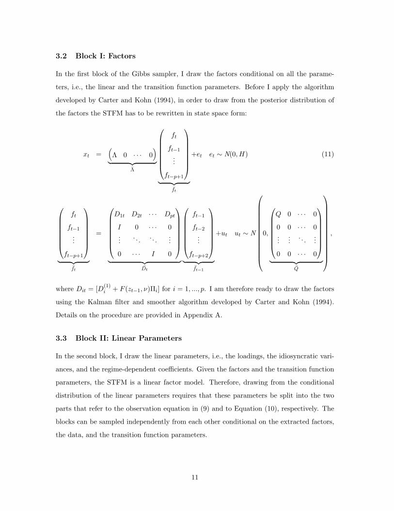
3.2 Block I: Factors

In the first block of the Gibbs sampler, I draw the factors conditional on all the parame-

ters, i.e., the linear and the transition function parameters. Before I apply the algorithm

developed by Carter and Kohn (1994), in order to draw from the posterior distribution of

the factors the STFM has to be rewritten in state space form:

xt =(

Λ 0 · · · 0)

︸︷︷︸

Λ

ft

ft−1

...

ft−p+1

︸︷︷︸

ft

+et et ∼ N(0, H) (11)

ft

ft−1

...

ft−p+1

︸︷︷︸

ft

=

D1t D2t · · · Dpt

I 0 · · · 0...

. . .. . .

...

0 · · · I 0

︸︷︷︸

Dt

ft−1

ft−2

...

ft−p+2

︸︷︷︸

ft−1

+ut ut ∼ N

0,

Q 0 · · · 0

0 0 · · · 0...

.... . .

...

0 0 · · · 0

︸︷︷︸

Q

,

where Dit = [D(1)i + F (zt−1, ν)Πi] for i = 1, ..., p. I am therefore ready to draw the factors

using the Kalman filter and smoother algorithm developed by Carter and Kohn (1994).

Details on the procedure are provided in Appendix A.

3.3 Block II: Linear Parameters

In the second block, I draw the linear parameters, i.e., the loadings, the idiosyncratic vari-

ances, and the regime-dependent coefficients. Given the factors and the transition function

parameters, the STFM is a linear factor model. Therefore, drawing from the conditional

distribution of the linear parameters requires that these parameters be split into the two

parts that refer to the observation equation in (9) and to Equation (10), respectively. The

blocks can be sampled independently from each other conditional on the extracted factors,

the data, and the transition function parameters.

11

Loadings and Idiosyncratic Variances

First, I draw the loadings, Λ, and the idiosyncratic variances, H. Conditional on the factors

and the transition function parameters, ν, Equation (9) represents simply N normal linear

regression models, and therefore the conditional posterior distributions are of standard

forms. Since the idiosyncratic errors, E, are independent across equations, the sampling

can be implemented one equation at a time. Note that the subscript n refers to the n-th

equation and that σ2n denotes the n-th diagonal element of H.

Using an improper prior for the idiosyncratic variances might result in a Bayesian ana-

logue of the Heywood problem, which takes the form of multi-modality of the posterior

of σ2n with one mode lying at 0 (Martin and McDonald (1975)). To avoid this potential

problem, I assume natural conjugate priors:

λn ∼ N(λn, σ2nV n)

σ2n ∼ IG(v/2, δ/2).

The variance of the normal prior for λn depends on σn because this allows joint drawing of

Λ and σ1, ..., σN .

Combining the likelihood of the STFM, which is given in Appendix A, with the prior

distributions, I obtain the following posterior distributions for Λ and σ2n:

λn|σ2n, X, F, ν ∼ N(λn, σ

2nV n)

σ2n|X,F, ν ∼ IG(v/2, δ/2),

where

λn = V n(V−1n λn + F ′Fλn)

V n = (V −1n + F ′F )−1

δ = vδ + e′nen + (λn − λn)′(V n + (F ′F )−1)−1(λn − λn)

v = T + v.

Variables with a hat refer to their respective ordinary least-squares estimates, i.e., λn =

12

(F ′F )−1F ′xn and en = xn − Fλn.

Regime-Dependent Coefficients

The second part refers to Equation (10), which is the STVAR of the factors. As mentioned

earlier, conditional on the factors and the transition function parameters, Equation (8)

becomes a multivariate regression and, hence, conditional posterior distributions can be

obtained in their standard forms. Since I assume the covariance matrix, Q, to be the

identity matrix, I only need to draw the regime-dependent coefficients, i.e., D(1)1 ,...,D

(1)p ,

Π1,...,Πp.

Since I do not have any strong a priori beliefs about the parameter values of D, I

choose the uninformative Jeffreys prior. Combining the likelihood with the prior, I obtain

a standard posterior distribution for vec(D) = d:

d|Q,X,F, ν ∼ N(d, V d

)

d = vec((

WST ′WST)−1

WST ′F)

V d = Q⊗(WST ′WST

)−1.

To ensure stationarity, I truncate the draws of D(1) and D(2) = Π + D(1). I discard the

draws whenever not all of the roots of the characteristic polynomials D(1)(L), D(2)(L), as

well as Dt(L), lie outside the unit circle.

3.4 Block III: Transition Function Parameters

In the last block of the Gibbs sampler, I draw the transition function parameters, i.e., the

smoothness parameter, γ, and the threshold value, c. Since their full conditional distribution

has no known form, I update them jointly using the Metropolis-Hastings algorithm following

Lopes and Salazar (2006). I assume similar priors as proposed by Lopes and Salazar (2006):

γ ∼ G(a, b)

c ∼ N(mc, σ2c ).

13

For given starting values (γ(0), c(0)) at iteration s of the Gibbs sampler, the Metropolis-

Hastings algorithm consists of two steps.

Step 1:

I generate draws from the following proposal densities:

γ∗ ∼ G(

(γ(s−1))2/∆γ ,∆γ/γ(s−1)

)

c∗ ∼ N(

c(s−1),∆c

)

.

The normal proposal density is truncated at the interval [cA, cB] with F (cA) = 0.05 and

F (cB) = 0.95, where F is the empirical distribution of the transition variable, z.

Step 2:

I set (γ(s), c(s)) = (γ∗, c∗) with probability α(γ∗, c∗|γ(s−1), c(s−1)) = min {1, A}, where

A =

∏Tt=1 pN (xt|f

∗t ,Λ

∗, D(1)(L)∗, D(2)(L)∗, Q∗)∏T

t=1 pN (xt|ft, zt−1,Λ, D(1)(L), D(2)(L), Q)

pG(γ∗|a, b)pN (c∗|mc, σ

2c )

pG(γ(s−1)|a, b)pN (c(s−1)|mc, σ2c )

×pG

(γ(s−1)|(γ∗)2/∆γ ,∆γ/γ

∗)

pG(γ∗|(γ(s−1))2/∆γ ,∆γ/γ(s−1)

)

Φ(cB−c(s−1)

√∆c

)

− Φ(cA−c(s−1)

√∆c

)

Φ(cB−c∗√

∆c

)

− Φ(cA−c∗√

∆c

) .

Otherwise (γ(s), c(s)) = (γ(s−1), c(s−1)). Therefore, A is the product of the likelihood ratio,

the prior ratio, and the proposal ratio. pN and pG denote the probability density function

of the normal and gamma, respectively. Φ(.) denotes the cumulative distribution function

of the standard normal distribution. ∆γ and ∆c are adjusted on the fly for the burn-in

period to generate an acceptance probability, which lies between 10% and 50%.

4 Empirical Results

In this section, I report the results of the analysis. First, I discuss the choice of the transition

variable. Then, the data, the model specification, the identification of the monetary policy

shock, and the choice of the prior hyperparameters are described. Next, I analyze the

convergence of the proposed Gibbs sampler algorithm, followed by estimation results of the

transition function. Finally, I report results for the persistence of shocks among the different

regimes and regime-dependent impulse responses to the monetary policy shock.

14

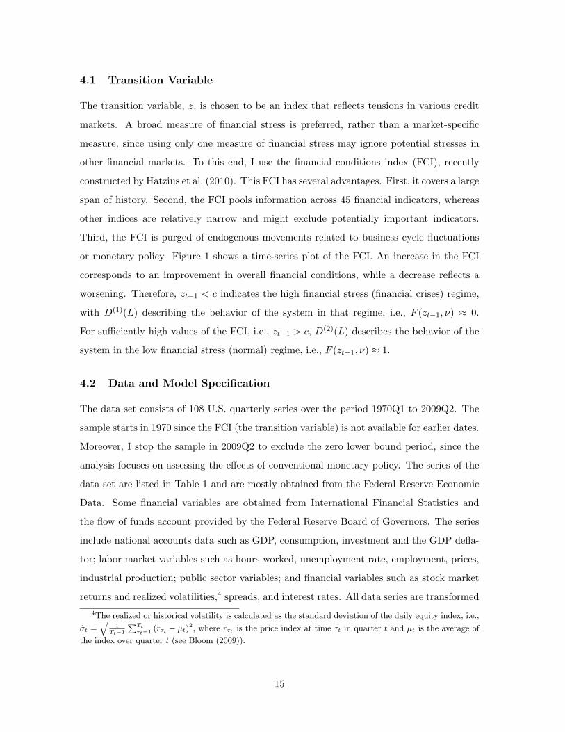
4.1 Transition Variable

The transition variable, z, is chosen to be an index that reflects tensions in various credit

markets. A broad measure of financial stress is preferred, rather than a market-specific

measure, since using only one measure of financial stress may ignore potential stresses in

other financial markets. To this end, I use the financial conditions index (FCI), recently

constructed by Hatzius et al. (2010). This FCI has several advantages. First, it covers a large

span of history. Second, the FCI pools information across 45 financial indicators, whereas

other indices are relatively narrow and might exclude potentially important indicators.

Third, the FCI is purged of endogenous movements related to business cycle fluctuations

or monetary policy. Figure 1 shows a time-series plot of the FCI. An increase in the FCI

corresponds to an improvement in overall financial conditions, while a decrease reflects a

worsening. Therefore, zt−1 < c indicates the high financial stress (financial crises) regime,

with D(1)(L) describing the behavior of the system in that regime, i.e., F (zt−1, ν) ≈ 0.

For sufficiently high values of the FCI, i.e., zt−1 > c, D(2)(L) describes the behavior of the

system in the low financial stress (normal) regime, i.e., F (zt−1, ν) ≈ 1.

4.2 Data and Model Specification

The data set consists of 108 U.S. quarterly series over the period 1970Q1 to 2009Q2. The

sample starts in 1970 since the FCI (the transition variable) is not available for earlier dates.

Moreover, I stop the sample in 2009Q2 to exclude the zero lower bound period, since the

analysis focuses on assessing the effects of conventional monetary policy. The series of the

data set are listed in Table 1 and are mostly obtained from the Federal Reserve Economic

Data. Some financial variables are obtained from International Financial Statistics and

the flow of funds account provided by the Federal Reserve Board of Governors. The series

include national accounts data such as GDP, consumption, investment and the GDP defla-

tor; labor market variables such as hours worked, unemployment rate, employment, prices,

industrial production; public sector variables; and financial variables such as stock market

returns and realized volatilities,4 spreads, and interest rates. All data series are transformed

4The realized or historical volatility is calculated as the standard deviation of the daily equity index, i.e.,

σt =√

1Tt−1

∑

Tt

τt=1 (rτt − µt)2, where rτt is the price index at time τt in quarter t and µt is the average of

the index over quarter t (see Bloom (2009)).

15

to reach stationarity. A list of transformations applied to the variables is given in the fourth

column of Table 1. Moreover, I set the number of factors to 4. Since the number of factors

determines the number of structural shocks in the STFM framework described here, this

choice corresponds to my preferred monetary policy identification scheme (see Section 4.3).

However, I experimented with specifications containing 3, 5 or 6 factors and the results I

obtained are very similar. Finally, I report results based on a lag length of one quarter, i.e.,

p = 1. I tried several versions with different lag lengths, but the results compared to the

ones reported here do not differ much.5

4.3 Identification of the Monetary Policy Shock

Following most of the literature, I assume a recursive or Cholesky scheme to identify a

conventional monetary policy shock (e.g., Sims (1992), Bernanke et al. (2005), and Chris-

tiano et al. (1999)). Equation (5) in Section 2 becomes a representation of the macroeco-

nomic variables, xt, in terms of structural shocks assuming a Cholesky identification scheme.

Therefore, the choice and order of the first r variables of my data set become relevant for

identification. Ordering the federal funds rate fourth in my data set, I assume that a mone-

tary policy shock has no contemporaneous effects on the first three variables of the data set.

I order GDP, the GDP deflator, and the CPI before the federal funds rate. Consequently,

under this ordering, GDP and prices react only with a lag to a monetary policy shock. The

CPI is ordered before the federal funds rate, since its inclusion can mitigate the price puzzle

(Eichenbaum (1992)).

4.4 Prior Choices

In choosing the hyperparameters for the priors of the loadings and idiosyncratic variances,

first, following, for example, Lopes and West (2004) and Bernanke et al. (2005), I choose a

vague prior for λn, i.e., λn = 0r×1, V n = Ir; second, the hyperparameters for σ2n are defined

as v = 0.001 and δ = 6 (see, for example, Otrok and Whiteman (1998) and Bernanke et al.

(2005)). These values produce a quite diffuse though proper prior.

Concerning the priors of the transition function parameters γ and c, the Gibbs sampling

5Note that, with increasing lag length, the number of degrees of freedom in each regime decreases. Toavoid the curse of dimensionality problem (especially in the high financial stress regime), the model isestimated using a higher prior mean of the threshold parameter.

16

algorithm is sensitive to the choice of hyperparameters. In particular, if the priors are

not sufficiently informative, the algorithm has difficulties converging. Therefore, I choose

relatively informative hyperparameter values in order to obtain well-mixing Markov chains

and an adequate acceptance rate. Typically, the data are not very informative on the shape

parameter, since a wide range of values of γ will lead to similar shapes of the transition

function (Deschamps (2008) and Terasvirta (1994)). Here I choose the hyperparameters,

a and b, of the prior for γ such that the mean of γ is equal to 3 and the variance is

equal to 0.1. To set the values of the hyperparameters for c, consider Figure 1, which

plots the FCI. Since I am interested in high financial stress episodes/financial crises, it

seems intuitive that I choose the prior mean of c in such a way that mainly financial crises

episodes are considered for the estimation of D(1). Therefore, I choose mc = −1.35 and

σ2c = 0.01. This allows me to partly exclude the low values of the FCI at the beginning of

the 1980s that originated from monetary policy that was responsible for very high interest

rates. Nevertheless, since the threshold parameter provides the point around which the

dynamics of the model change, I also experiment with choosing different prior means of c,

i.e., mc = {−1.2,−1.1,−1.0,−0.9,−0.8}. Results are robust to these prior choices.

4.5 Convergence

To make sure that the results are based on converged simulations, I follow various strategies.

First, all my results are based on 20,000 draws of the Metropolis-within-Gibbs sampler,

where the first 4,000 draws are discarded as burn-in. Second, I thin the draws by considering

only every fourth draw to reduce possible autocorrelations of the sequence (since I have a

Metropolis-Hastings step). Third, the Gibbs sampler is run several times to compare the

results obtained each time assuring that the chain is converging to the same stationary

distribution. Moreover, I assess convergence visually by checking the trace plots, which

show the evolution of draws of the parameters and the log-likelihood. This is helpful for

checking whether there are jumps in the level and variance of the respective parameter.

Furthermore, to assure that the Gibbs sampler has moved to its target distribution, I plot

the estimated factors obtained in the first half of simulations against the ones obtained in the

second half of the sampler (see Figure 2). Small deviations show that the simulated chain

has converged. Finally, to assess the precision of the Gibbs sampler, I plot the estimated

17

factors with their 95% confidence bands (Figure 3). Since the estimated factors of the first

and second halves of the simulations are nearly identical and the bands of the estimated

factors are tight, the chain seems to converge properly.

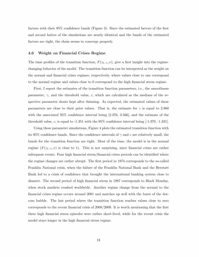
4.6 Weight on Financial Crises Regime

The time profiles of the transition function, F (zt−1, ν), give a first insight into the regime-

changing behavior of the model. The transition function can be interpreted as the weight on

the normal and financial crises regimes, respectively, where values close to one correspond

to the normal regime and values close to 0 correspond to the high financial stress regime.

First, I report the estimates of the transition function parameters, i.e., the smoothness

parameter, γ, and the threshold value, c, which are calculated as the medians of the re-

spective parameter draws kept after thinning. As expected, the estimated values of these

parameters are close to their prior values. That is, the estimate for γ is equal to 2.860

with the associated 95% confidence interval being [2.276, 3.566], and the estimate of the

threshold value, c, is equal to -1.351 with the 95% confidence interval being [-1.370, -1.331].

Using these parameter simulations, Figure 4 plots the estimated transition function with

its 95% confidence bands. Since the confidence intervals of γ and c are relatively small, the

bands for the transition function are tight. Most of the time, the model is in the normal

regime (F (zt−1, ν) is close to 1). This is not surprising, since financial crises are rather

infrequent events. Four high financial stress/financial crises periods can be identified where

the regime changes are rather abrupt. The first period in 1974 corresponds to the so-called

Franklin National crisis, when the failure of the Franklin National Bank and the Herstatt

Bank led to a crisis of confidence that brought the international banking system close to

disaster. The second period of high financial stress in 1987 corresponds to Black Monday,

when stock markets crashed worldwide. Another regime change from the normal to the

financial crises regime occurs around 2001 and matches up well with the burst of the dot-

com bubble. The last period where the transition function reaches values close to zero

corresponds to the recent financial crisis of 2008/2009. It is worth mentioning that the first

three high financial stress episodes were rather short-lived, while for the recent crisis the

model stays longer in the high financial stress regime.

18

4.7 Persistence among Regimes

One may expect to find a difference in the persistence of effects between the normal and

the financial crises regimes. The persistence of effects depends on the eigenvalues of the

companion form of the regime-dependent coefficient matrices. More specifically, the closer

the eigenvalues are to unity, the higher is the persistence of effects following shocks. In the

case of greater-than-unity eigenvalues, the impulse responses would be explosive. Note that

the latter case is automatically excluded, since I discard draws of the coefficient matrices

that are associated with eigenvalues bigger than or equal to one.

First, I report the results for the maximum eigenvalues of the extreme regime lag poly-

nomials, D(1)(L) and D(2)(L), that correspond to F (zt−1, ν) = 0 and F (zt−1, ν) = 1,

respectively. The median of the maximum eigenvalue associated with the draws of D(1)(L)

kept after thinning is equal to 0.928, with the 68% confidence interval being [0.821,0.979].

Moreover, for the draws of D(2)(L), the median of the maximum eigenvalue is 0.644 and its

confidence interval is given by [0.551,0.742]. It seems that the persistence of shocks indeed

varies in the two regimes.

Next, the maximum eigenvalues associated with Dt(L) are obtained for each draw kept.

This provides me with a plot of the median and 68% confidence interval of the maximum

eigenvalues for each point in time t (see Figure 5). Whenever the model is in the financial

crises regime (i.e., in 1974, 1987, 2001 and 2008/2009), the plot shows a high spike for the

maximum eigenvalue. Therefore, it seems that shocks have more persistent effects during

financial crises than in normal times.

4.8 Monetary Policy Shock

Impulse-response functions are the key statistics to shed light on whether monetary policy

transmission is different during normal times and times of high financial stress. This section

reports the results for the regime-dependent impulse responses of an expansionary monetary

policy shock. Note that I construct impulse responses to monetary policy shocks conditional

on a given regime. In other words, I assume that once the system is in a regime, it can

stay in that regime for a long time.6 Moreover, as in Auerbach and Gorodnichenko (2012),

6The advantage of this approach is that, once a regime is fixed, the model is linear and hence impulseresponses are not functions of history (for details, see Koop et al. (1996)). Nevertheless, allowing for feedbackfrom changes in z into the dynamics of macroeconomic variables, I consider an interesting issue, which is

19

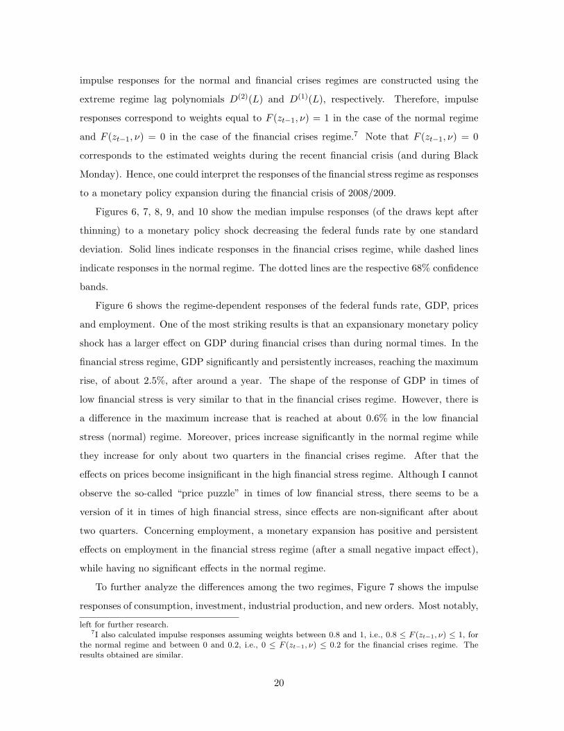
impulse responses for the normal and financial crises regimes are constructed using the

extreme regime lag polynomials D(2)(L) and D(1)(L), respectively. Therefore, impulse

responses correspond to weights equal to F (zt−1, ν) = 1 in the case of the normal regime

and F (zt−1, ν) = 0 in the case of the financial crises regime.7 Note that F (zt−1, ν) = 0

corresponds to the estimated weights during the recent financial crisis (and during Black

Monday). Hence, one could interpret the responses of the financial stress regime as responses

to a monetary policy expansion during the financial crisis of 2008/2009.

Figures 6, 7, 8, 9, and 10 show the median impulse responses (of the draws kept after

thinning) to a monetary policy shock decreasing the federal funds rate by one standard

deviation. Solid lines indicate responses in the financial crises regime, while dashed lines

indicate responses in the normal regime. The dotted lines are the respective 68% confidence

bands.

Figure 6 shows the regime-dependent responses of the federal funds rate, GDP, prices

and employment. One of the most striking results is that an expansionary monetary policy

shock has a larger effect on GDP during financial crises than during normal times. In the

financial stress regime, GDP significantly and persistently increases, reaching the maximum

rise, of about 2.5%, after around a year. The shape of the response of GDP in times of

low financial stress is very similar to that in the financial crises regime. However, there is

a difference in the maximum increase that is reached at about 0.6% in the low financial

stress (normal) regime. Moreover, prices increase significantly in the normal regime while

they increase for only about two quarters in the financial crises regime. After that the

effects on prices become insignificant in the high financial stress regime. Although I cannot

observe the so-called “price puzzle” in times of low financial stress, there seems to be a

version of it in times of high financial stress, since effects are non-significant after about

two quarters. Concerning employment, a monetary expansion has positive and persistent

effects on employment in the financial stress regime (after a small negative impact effect),

while having no significant effects in the normal regime.

To further analyze the differences among the two regimes, Figure 7 shows the impulse

responses of consumption, investment, industrial production, and new orders. Most notably,

left for further research.7I also calculated impulse responses assuming weights between 0.8 and 1, i.e., 0.8 ≤ F (zt−1, ν) ≤ 1, for

the normal regime and between 0 and 0.2, i.e., 0 ≤ F (zt−1, ν) ≤ 0.2 for the financial crises regime. Theresults obtained are similar.

20

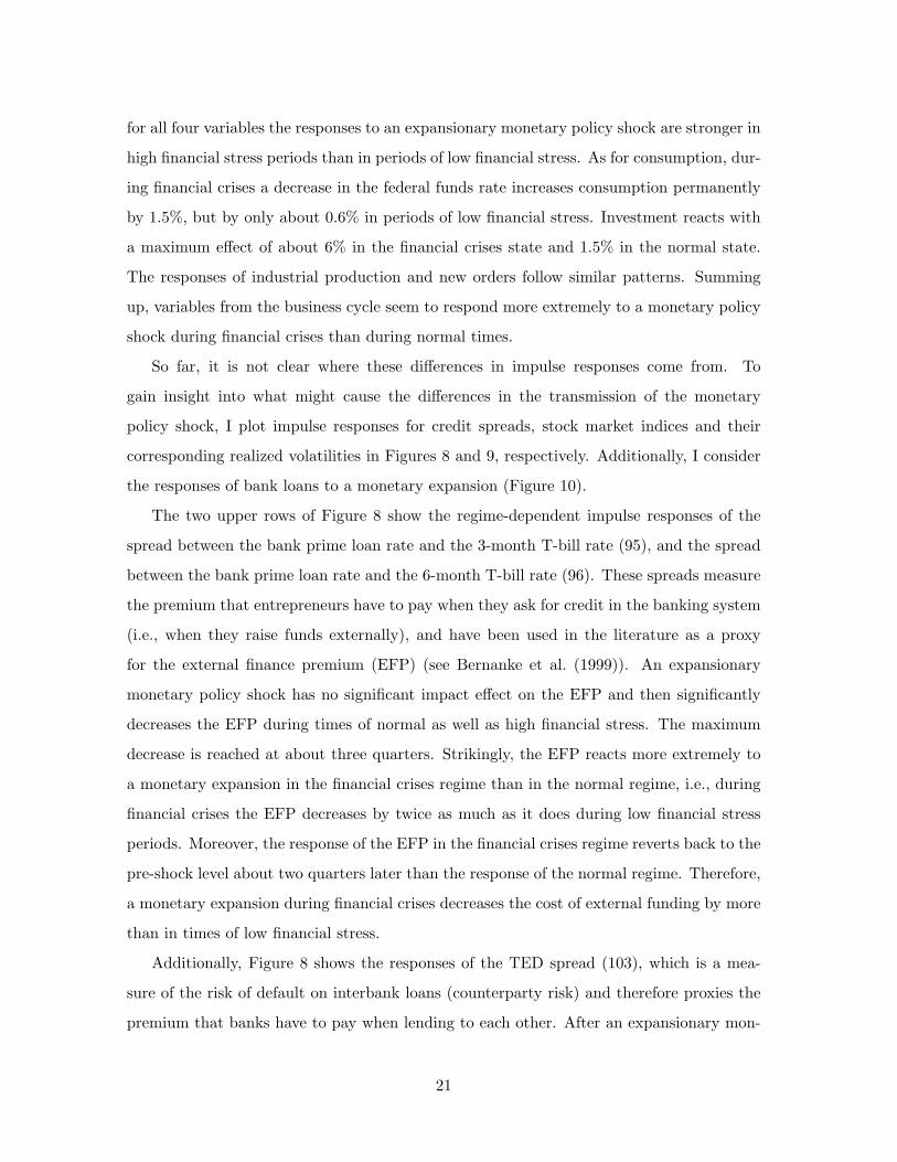
for all four variables the responses to an expansionary monetary policy shock are stronger in

high financial stress periods than in periods of low financial stress. As for consumption, dur-

ing financial crises a decrease in the federal funds rate increases consumption permanently

by 1.5%, but by only about 0.6% in periods of low financial stress. Investment reacts with

a maximum effect of about 6% in the financial crises state and 1.5% in the normal state.

The responses of industrial production and new orders follow similar patterns. Summing

up, variables from the business cycle seem to respond more extremely to a monetary policy

shock during financial crises than during normal times.

So far, it is not clear where these differences in impulse responses come from. To

gain insight into what might cause the differences in the transmission of the monetary

policy shock, I plot impulse responses for credit spreads, stock market indices and their

corresponding realized volatilities in Figures 8 and 9, respectively. Additionally, I consider

the responses of bank loans to a monetary expansion (Figure 10).

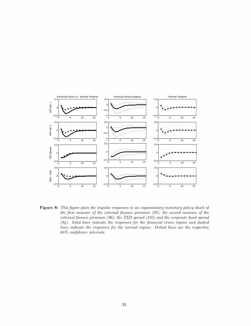
The two upper rows of Figure 8 show the regime-dependent impulse responses of the

spread between the bank prime loan rate and the 3-month T-bill rate (95), and the spread

between the bank prime loan rate and the 6-month T-bill rate (96). These spreads measure

the premium that entrepreneurs have to pay when they ask for credit in the banking system

(i.e., when they raise funds externally), and have been used in the literature as a proxy

for the external finance premium (EFP) (see Bernanke et al. (1999)). An expansionary

monetary policy shock has no significant impact effect on the EFP and then significantly

decreases the EFP during times of normal as well as high financial stress. The maximum

decrease is reached at about three quarters. Strikingly, the EFP reacts more extremely to

a monetary expansion in the financial crises regime than in the normal regime, i.e., during

financial crises the EFP decreases by twice as much as it does during low financial stress

periods. Moreover, the response of the EFP in the financial crises regime reverts back to the

pre-shock level about two quarters later than the response of the normal regime. Therefore,

a monetary expansion during financial crises decreases the cost of external funding by more

than in times of low financial stress.

Additionally, Figure 8 shows the responses of the TED spread (103), which is a mea-

sure of the risk of default on interbank loans (counterparty risk) and therefore proxies the

premium that banks have to pay when lending to each other. After an expansionary mon-

21

etary policy, the TED spread decreases on impact and reverts back to the pre-shock level

after about a year in both regimes. The responses of the normal and the financial crises

regimes are nearly identical in the case of the TED spread. This suggests that even though

a monetary expansion decreases the counterparty risk in both regimes, its effects are not

asymmetric. Finally, the last row of Figure 8 shows the regime-dependent impulse response

of the Baa-Aaa spread (94), i.e., the corporate bond spread. A monetary policy shock

increases the spread slightly on impact in both regimes. While in the normal regime the

response of the corporate bond spread stabilizes at the pre-shock level after about a year,

the response of the financial stress regime turns negative after about two quarters and re-

verts back to the pre-shock level after about two years. Therefore, the monetary expansion

decreases the cost of bond financing via lower-rated bonds during times of financial stress.

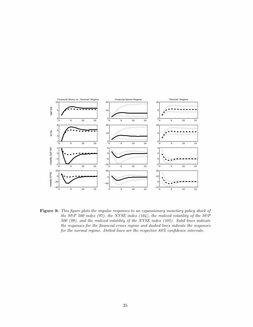
Figure 9 shows the regime-dependent impulse responses of the S&P 500 and NYSE

price index, and of their respective realized volatilities. An expansionary monetary policy

shock significantly and permanently increases both stock price indices. The S&P 500 index

increases by about 2% on impact in both regimes. While the response of the financial crises

state reaches its maximum increase of about 7.5% after a year and then stabilizes at a little

bit less than 7%, the response of the normal state stabilizes at around 5% after two quarters.

A very similar pattern arises for the regime-dependent responses of the NYSE index. Since

the stock market indices can be seen as a proxy for entrepreneurs’ wealth, a monetary

expansion during financial crises increases the worth of a firm by more than it does during

periods of low financial stress. Moreover, a monetary policy shock seems to have no effects

on the volatility of stocks in the normal regime, since the responses are not significantly

different from zero (except for a slightly positive effect on impact). Nevertheless, in the

financial crises regime, the response of the realized volatility significantly decreases after a

monetary expansion, reverting to the pre-shock level after about 1.5 years. This indicates

that a monetary expansion decreases the uncertainty regarding the value of assets during

financial crises, while it has no effect on this uncertainty in normal times.

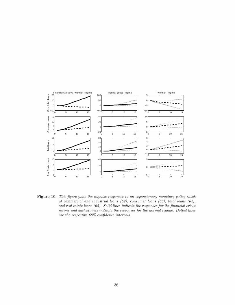
Finally, I consider the effects of a monetary expansion on several loans at commercial

banks (see Figure 10). A similar pattern arises for all the different types of loans. During

financial crises, commercial and industrial loans, consumer loans, total loans, and real

estate loans at commercial banks increase significantly after an expansionary monetary

22

policy shock. Conversely, I cannot observe any clear-cut effects on the different types of

loans in the normal regime. Responses of loans during times of low financial stress are

insignificant, except that one might argue that the response of consumer loans is slightly

increasing. Therefore, a monetary expansion has asymmetric effects on loans, i.e., while a

monetary expansion during normal times does not have any significant effects on loans, it

raises loans during financial crises.

These findings for the financial market variables have various implications. First, the

negative response of the credit risk spreads, i.e., EFP, in the financial crises as well as in the

normal regime, suggests that monetary policy and the premium that entrepreneurs have

to pay when they ask for external credit may be linked. Therefore, this finding provides

supportive evidence for the existence of a credit channel of monetary policy or the so-

called financial accelerator (see the seminal contributions of Bernanke and Gertler (1989),

Bernanke et al. (1996) and Bernanke et al. (1999)). The credit channel can be broken down

into two components: the balance-sheet channel and the bank-lending channel (Bernanke

and Gertler (1995)). Consequently, the positive response of entrepreneurs’ wealth, i.e., the

S&P 500 and NYSE index, in both regimes supports the potential existence of a balance-

sheet transmission channel. More specifically, the balance-sheet channel suggests that an

expansionary monetary policy shock increases the net worth of borrowers via the increase

in asset prices, forcing down the EFP, which decreases the effective cost of credit, and

therefore further stimulates investment and output. I observe these balance-sheet effects

for the high financial stress as well as for the low financial stress regime, with effects being

stronger during times of high financial stress. Moreover, a monetary policy expansion may

also affect the EFP by shifting the supply of intermediated credit, in particular, loans by

commercial banks. Consequently, the positive response of loans in the financial crises regime

may suggest the existence of a bank-lending channel at least during financial crises, when

financial market imperfections are high.

Second, and more important for the question at hand, is the fact that effects on the

EFP are stronger in the financial crises regime than in the normal regime. Moreover, stock

prices, volatilities, and loans are affected more in the case of high financial stress. This may

indicate that the financial accelerator is stronger when the financial fundamentals, e.g., the

entrepreneurs’ wealth, are low, that is, during financial crises. This possibility of non-linear

23

balance-sheet effects was discussed for example in Bernanke and Gertler (1989), Gertler

and Gilchrist (1994), and Bernanke et al. (1996). More specifically, in a high financial

stress regime, an expansionary monetary policy shock increases asset prices and decreases

the EFP by more than in the low financial stress regime. This translates into a stronger

increase of investment, output, and other variables describing the state of the economy such

as consumption, industrial production, employment, and new orders.

5 Conclusion

This paper investigates whether monetary policy transmission during financial crises differs

from what is usually observed in low financial stress or normal times. In order to do so,

I introduce the STFM, which is a regime-dependent factor model where the transition

between states (normal and high financial stress times) depends on a financial conditions

index.

My analysis shows substantial evidence that the transmission of a conventional monetary

policy shock is different in times of financial crises. More specifically, I find that a monetary

expansion during financial crises has stronger and more persistent effects on macroeconomic

variables such as output, consumption, and investment than during normal times. These

differences in effects among the regimes seem to originate from non-linearities in the credit

channel. That is, a monetary expansion increases asset prices and loans by more during

financial crises than in normal times, leading to a higher decrease in the EFP which, in

turn, provokes the stronger effects on macroeconomic variables such as output, investment,

and consumption.

24

References

Auerbach, A. J. and Gorodnichenko, Y. (2012). Measuring the output responses to fiscal

policy, American Economic Journal of Economic Policy 4(2): 1–27.

Bernanke, B., Boivin, J. and Eliasz, P. S. (2005). Measuring the effects of monetary policy:

A factor-augmented vector autoregressive (FAVAR) approach, The Quarterly Journal of

Economics 120(1): 387–422.

Bernanke, B. S. and Gertler, M. (1989). Agency costs, collateral, and business fluctuations,

American Economic Review (79): 14–31.

Bernanke, B. S. and Gertler, M. (1995). Inside the black box: The credit channel of

monetary policy transmission, Journal of Economic Perspectives 9(4): 27–48.

Bernanke, B. S., Gertler, M. and Gilchrist, S. (1996). The financial accelerator and the

flight to quality, Review of Economics and Statistics 78(1): 1–15.

Bernanke, B. S., Gertler, M. and Gilchrist, S. (1999). The financial accelerator in a quan-

titative business cycle framework, in J. Taylor and M. Woodford (eds), The Handbook of

Macroeconomics, Elsevier Science B. V., Amsterdam, pp. 1341–1393.

Bloom, N. (2009). The impact of uncertainty shocks, Econometrica 77(3): 623–685.

Carter, C. and Kohn, R. (1994). On Gibbs sampling for state space models, Biometrika

81: 541–553.

Christiano, L. J., Eichenbaum, M. and Evans, C. L. (1999). Monetary policy shocks: What

have we learned and to what end?, in J. B. Taylor and M. Woodford (eds), Handbook of

Macroeconomics, Vol. 1 of Handbook of Macroeconomics, Elsevier, chapter 2, pp. 65–148.

Davig, T. and Hakkio, C. (2010). What is the effect of financial stress on economic activity,

Federal Reserve Bank of Kansas City Economic Review 2nd quarter.

Del Negro, M. and Schorfheide, F. (2011). Bayesian macroeconometrics, in J. Geweke,

G. Koop and H. van Dijk (eds), The Oxford Handbook of Bayesian Econometrics, Oxford

University Press.

25

Deschamps, P. J. (2008). Comparing smooth transition and Markov switching autoregressive

models of US unemployment, Journal of Applied Econometrics 23(4): 435–462.

Eichenbaum, M. (1992). Comment on “Interpreting the macroeconomic time series facts:

The effects of monetary policy”: by Christopher Sims, European Economic Review

36(5): 1001–1011.

Forni, M., Domenico, G., Lippi, M. and Reichlin, L. (2009). Opening the black box: Struc-

tural factor models with large cross sections, Econometric Theory 25(05): 1319–1347.

Gertler, M. and Gilchrist, S. (1994). Monetary policy, business cycles, and the behavior of

small manufacturing firms, Quarterly Journal of Economics 109(2): 309–40.

Granger, C. W. and Terasvirta, T. (1993). Modelling Nonlinear Economic Relationships,

Oxford University Press, New York.

Hatzius, J., Hooper, P., Mishkin, F., Schoenholtz, K. and Watson, M. W. (2010). Financial

conditions indexes: A fresh look after the financial crisis, NBER Working Paper No.

16150 .

Hubrich, K. and Tetlow, R. J. (2012). Financial stress and economic dynamics: The trans-

mission of crises, Finance and Economics Discussion Series No. 2012-82, Federal Reserve

Board.

Kim, C. J. and Nelson, C. R. (1999). State-Space Models with Regime Switching: Classical

and Gibbs-Sampling Approaches with Applications, Vol. 1 of MIT Press Books, The MIT

Press.

Koop, G., Pesaran, M. H. and Potter, S. M. (1996). Impulse response analysis in nonlinear

multivariate models, Journal of Econometrics 74(1): 119–147.

Krugman, P. (2008). Depression economics returns, The New York Times .

Lopes, H. F. and Salazar, E. (2006). Bayesian model uncertainty in smooth transition

autoregressions, Journal of Time Series Analysis 27(1): 99–117.

Lopes, H. F. and West, M. (2004). Bayesian model assessment in factor analysis, Statistica

Sinica 14: 41–67.

26

Martin, J. and McDonald, R. (1975). Bayesian estimation in unrestricted factor analysis:

A treatment for Heywood cases, Psychometrika 40(4): 505–517.

Mishkin, F. S. (2009). Is monetary policy effective during financial crises?, American Eco-

nomic Review 99(2): 573–77.

Otrok, C. and Whiteman, C. H. (1998). Bayesian leading indicators: Measuring and pre-

dicting economic conditions in Iowa, International Economic Review 39(4): 997–1014.

Ravn, S. H. (2014). Asymmetric monetary policy towards the stock market: A DSGE

approach, Journal of Macroeconomics 39, Part A(0): 24–41.

Sims, C. A. (1992). Interpreting the macroeconomic time series facts: The effects of mone-

tary policy, European Economic Review 36(5): 975–1000.

Stock, J. and Watson, M. W. (2012). Disentangling the channels of the 2007-2009 recession,

NBER Working Paper No. 18094.

Terasvirta, T. (1994). Specification, estimation, and evaluation of smooth transition au-

toregressive models, Journal of the American Statistical Association 89: 208–218.

Weise, C. L. (1999). The asymmetric effects of monetary policy: A nonlinear vector autore-

gression approach, Journal of Money, Credit and Banking 31(1): 85–108.

27

Series Mnemonic Description Transformation1 GDPC1 Real Gross Domestic Product, 1 Decimal 52 GDPDEF Gross Domestic Product: Implicit Price Deflator 63 CPIAUCSL Consumer Price Index For All Urban Consumers: All Items 64 FEDFUNDS Effective Federal Funds Rate 25 GNPC96 Real Gross National Product 56 NICUR/GDPDEF National Income/GDPDEF 57 DPIC96 Real Disposable Personal Income 58 OUTNFB Nonfarm Business Sector: Output 59 FINSLC1 Real Final Sales of Domestic Product 5

10 FPIC1 Real Private Fixed Investment 511 PRFIC1 Real Private Residential Fixed Investment 512 PNFIC1 Real Private Nonresidential Fixed Investment 513 GPDIC1 Real Gross Private Domestic Investment 514 PCECC96 Real Personal Consumption Expenditures 515 PCNDGC96 Real Personal Consumption Expenditures: Nondurable Goods 516 PCDGCC96 Real Personal Consumption Expenditures: Durable Goods 517 PCESVC96 Real Personal Consumption Expenditures: Services 518 GPSAVE/GDPDEF Gross Private Saving/GDP Deflator 519 FGCEC1 Real Federal Consumption Expenditures & Gross Investment 520 FGEXPND/GDPDEF Federal Government: Current Expenditures/GDP deflator 521 FGRECPT/GDPDEF Federal Government Current Receipts/GDP deflator 522 FGDEF Federal Real Expend-Real Receipts 223 CBIC1 Real Change in Private Inventories 124 EXPGSC1 Real Exports of Goods & Services 525 IMPGSC1 Real Imports of Goods & Services 526 CP/GDPDEF Corporate Profits After Tax/GDP deflator 527 NFCPATAX/GDPDEF Nonfinancial Corporate Business: Profits After Tax/GDP deflator 528 CNCF/GDPDEF Corporate Net Cash Flow/GDP deflator 529 DIVIDEND/GDPDEF Net Corporate Dividends/GDP deflator 530 HOANBS Nonfarm Business Sector: Hours of All Persons 531 OPHNFB Nonfarm Business Sector: Output Per Hour of All Persons 532 UNLPNBS Nonfarm Business Sector: Unit Nonlabor Payments 533 ULCNFB Nonfarm Business Sector: Unit Labor Cost 534 WASCUR/CPI Compensation of Employees: Wages & Salary Accruals/CPI 535 COMPNFB Nonfarm Business Sector: Compensation Per Hour 636 COMPRNFB Nonfarm Business Sector: Real Compensation Per Hour 537 GDPCTPI Gross Domestic Product: Chain-type Price Index 638 GNPCTPI Gross National Product: Chain-type Price Index 639 GNPDEF Gross National Product: Implicit Price Deflator 640 INDPRO Industrial Production Index 541 IPBUSEQ Industrial Production: Business Equipment 542 IPCONGD Industrial Production: Consumer Goods 543 IPDCONGD Industrial Production: Durable Consumer Goods 544 IPFINAL Industrial Production: Final Products (Market Group) 545 IPMAT Industrial Production: Materials 546 IPNCONGD Industrial Production: Nondurable Consumer Goods 547 AWHMAN Average Weekly Hours: Manufacturing 248 AWOTMAN Average Weekly Hours: Overtime: Manufacturing 249 CIVPART Civilian Participation Rate 250 CLF16OV Civilian Labor Force 551 CE16OV Civilian Employment 552 USPRIV All Employees: Total Private Industries 553 USGOOD All Employees: Goods-Producing Industries 554 SRVPRD All Employees: Service-Providing Industries 5

Table 1: Transformations of xt: 1 = xt, 2 = ∆xt, 5 = ∆ log xt, 6 = ∆2 log xt

Continued...

28

Series Mnemonic Description Transformation55 UNEMPLOY Unemployed 556 UEMPMEAN Average (Mean) Duration of Unemployment 557 UNRATE Civilian Unemployment Rate 258 HOUST Housing Starts: Total: New Privately Owned Housing Units Started 559 M1SL M1 Money Stock 660 M2MSL M2 Minus 661 M2SL M2 Money Stock 662 BUSLOANS Commercial and Industrial Loans at All Commercial Banks 663 CONSUMER Consumer (Individual) Loans at All Commercial Banks 664 LOANINV Total Loans and Investments at All Commercial Banks 665 REALLN Real Estate Loans at All Commercial Banks 666 TOTALSL Total Consumer Credit Outstanding 667 CPIULFSL Consumer Price Index for All Urban Consumers: All Items Less Food 668 CPILEGSL Consumer Price Index for All Urban Consumers: All Items Less Energy 669 CPILFESL Consumer Price Index for All Urban Consumers: All Items Less Food & Energy 670 CPIENGSL Consumer Price Index for All Urban Consumers: Energy 671 CPIUFDSL Consumer Price Index for All Urban Consumers: Food 672 PPICPE Producer Price Index Finished Goods: Capital Equipment 673 PPICRM Producer Price Index: Crude Materials for Further Processing 674 PPIFCG Producer Price Index: Finished Consumer Goods 675 PPIFGS Producer Price Index: Finished Goods 676 OILPRICE Spot Oil Price: West Texas Intermediate 677 USNEDG US Manufacturers new Orders of durable Goods 578 USNOCG US New Orders of Consumer Goods & Materials 579 NAPMNOI US ISM Manufacturer Survey: New Orders Index 180 USCYLEAD US the Conference Board Leading Economic Indicators Index 581 GEXPND/GDPDEF Government Current Expenditures/ GDP deflator 582 GRECPT/GDPDEF Government Current Receipts/ GDP deflator 583 GDEF Governnent Real Expend-Real Receipts 284 GCEC1 Real Government Consumption Expenditures & Gross Investment 585 TB3MS 3-Month Treasury Bill: Secondary Market Rate 286 TB6MS 6-Month Treasury Bill: Secondary Market Rate 287 GS1 1-Year Treasury Constant Maturity Rate 288 GS10 10-Year Treasury Constant Maturity Rate 289 AAA Moody’s Seasoned Aaa Corporate Bond Yield 290 BAA Moody’s Seasoned Baa Corporate Bond Yield 291 MPRIME Bank Prime Loan Rate 292 GS10-FEDFUNDS 193 GS1-FEDFUNDS 194 BAA-AAA Default Rate Spread 195 MPRIME-TB3MS External Finance Premium 196 MPRIME-TB6MS Bank Prime Loan Rate minus 6-Month Treasury Bill 197 US500STK US Standard & Poor’s Index of 500 common Stocks 598 USSHRPRCF US Dow Jones Industrial Share Price Index 599 Realized Volatility of S&P 500 Index 1

100 LIBOR3M 3-Month US Deposit London Offer 2101 LIBOR6M 6-Month US Deposit London Offer 2102 LIBOR3M-FEDFUNDS 1103 LIBOR3M-TB3M TED spread 1104 NYSE US NYSE Composite Index 5105 Realized Volatility of NYSE Index 1106 EXCRESNS Excess Reserves of Depository Institutions 5107 ADJRESSL Adjusted Monetary Base 5108 Real Net Taxes 5

Table 1 (Continued): Transformations of xt: 1 = xt, 2 = ∆xt, 5 = ∆ log xt, 6 = ∆2 log xt

29

1970 1975 1980 1985 1990 1995 2000 2005 2010−4

−3

−2

−1

0

1

2

3

Figure 1: The black line shows the FCI of Hatzius et al. (2010). The red line is the estimatedthreshold value, c. The estimate has been calculated as the median of the thresholdvalue draws of the Metropolis-within-Gibbs sampler kept after thinning.

1970 1975 1980 1985 1990 1995 2000 2005 2010−4

−3

−2

−1

0

1

2

3Factor 1

1970 1975 1980 1985 1990 1995 2000 2005 2010−2

−1

0

1

2

3Factor 2

1970 1975 1980 1985 1990 1995 2000 2005 2010−3

−2

−1

0

1

2Factor 3

1970 1975 1980 1985 1990 1995 2000 2005 2010−3

−2

−1

0

1

2

3Factor 4

Figure 2: This figure plots the estimated factors obtained in the first half of the Gibbs sampleragainst the ones obtained in the second half. The estimates are calculated as themedian of the factor draws of the Gibbs sampler kept after thinning.

30

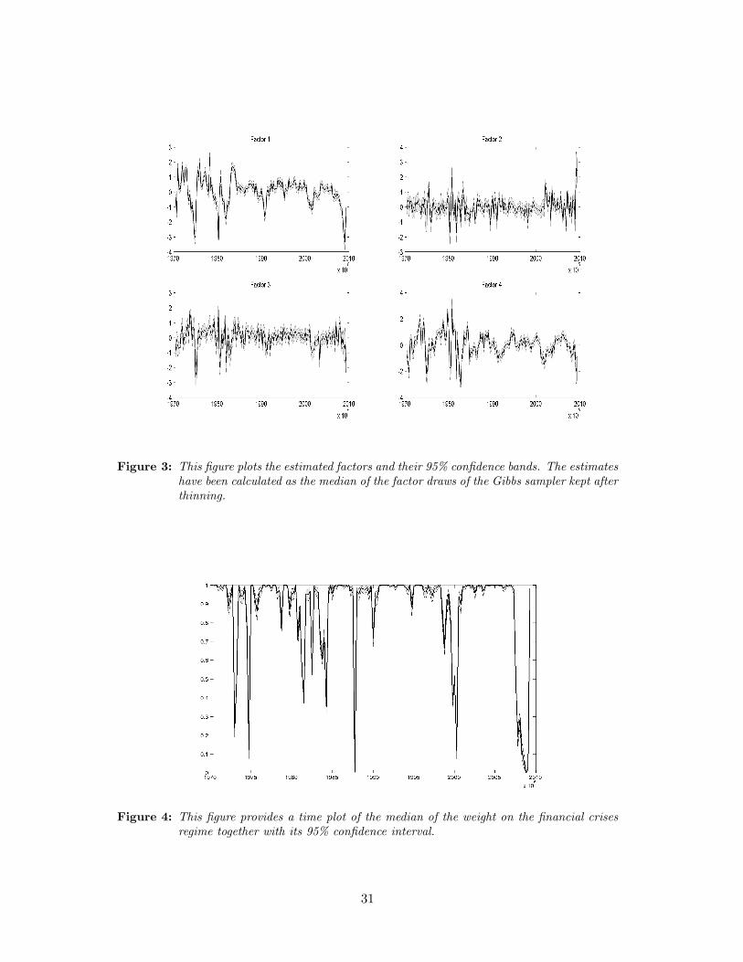
Figure 3: This figure plots the estimated factors and their 95% confidence bands. The estimateshave been calculated as the median of the factor draws of the Gibbs sampler kept afterthinning.

Figure 4: This figure provides a time plot of the median of the weight on the financial crisesregime together with its 95% confidence interval.

31

Figure 5: This figure provides a plot of the median of the maximum eigenvalues of Dt togetherwith its 68% confidence intervals over time.

0 5 10 15−2

0

2Financial Stress vs. "Normal" Regime

Fed

Fund

s R

ate

0 5 10 15−2

0

2

4

Financial Stress Regime

0 5 10 15−2

−1.5

−1

−0.5"Normal" Regime

0 5 10 150

1

2

3

GD

P

0 5 10 150

5

10

0 5 10 150

0.5

1

1.5

0 5 10 150

1

2

Pric

es

0 5 10 15−5

0

5

0 5 10 150

2

4

0 5 10 15−1

0

1

2

Em

ploy

men

t

0 5 10 15

0

2

4

0 5 10 15−0.5

0

0.5

Figure 6: This figure plots the impulse responses to an expansionary monetary policy shock ofthe federal funds rate (4), GDP (1), prices (2), and employment (51). Solid linesindicate the responses for the high financial stress regime and dashed lines indicatethe responses for the normal regime. Dotted lines are the respective 68% confidenceintervals.

32

0 2 4 6 8 10 12 14 160

0.5

1

1.5Financial Stress vs. "Normal" Regime

Co

nsu

mp

tio

n

0 2 4 6 8 10 12 14 160

1

2

3

4

5Financial Stress Regime

0 2 4 6 8 10 12 14 160

0.2

0.4

0.6

0.8

1"Normal" Regime

0 2 4 6 8 10 12 14 16−2

0

2

4

6

8

Inve

stm

en

t

0 2 4 6 8 10 12 14 16

0

10

20

30

0 2 4 6 8 10 12 14 16−1

0

1

2

3

4

0 2 4 6 8 10 12 14 16−1

0

1

2

3

4

5

Ind

ustr

ial P

rod

uctio

n

0 2 4 6 8 10 12 14 160

5

10

15

20

0 2 4 6 8 10 12 14 16−0.5

0

0.5

1

1.5

2

0 2 4 6 8 10 12 14 16

0

2

4

6

8

10

Ne

w O

rde

rs

0 2 4 6 8 10 12 14 160

10

20

30

0 2 4 6 8 10 12 14 16

0

1

2

3

4

Figure 7: This figure plots the impulse responses to an expansionary monetary policy shockof consumption (14), investment (10), industrial production (40), and new orders(78). Solid lines indicate the responses for the financial crises regime and dashedlines indicate the responses for the normal regime. Dotted lines are the respective68% confidence intervals.

33

0 5 10 15−0.5

0

0.5Financial Stress vs. "Normal" Regime

EFP

def

. 1

0 5 10 15−1

−0.5

0

0.5Financial Stress Regime

0 5 10 15−0.5

0

0.5"Normal" Regime

0 5 10 15−0.5

0

0.5

EFP

def

. 2

0 5 10 15−1

−0.5

0

0.5

0 5 10 15−0.5

0

0.5

0 5 10 15−0.5

0

0.5

TED

Spr

ead

0 5 10 15−0.5

0

0.5

0 5 10 15−0.5

0

0.5

0 5 10 15−0.5

0

0.5

BA

A −

AA

A

0 5 10 15−0.5

0

0.5

0 5 10 15−0.5

0

0.5

Figure 8: This figure plots the impulse responses to an expansionary monetary policy shock ofthe first measure of the external finance premium (95), the second measure of theexternal finance premium (96), the TED spread (103) and the corporate bond spread(94). Solid lines indicate the responses for the financial crises regime and dashedlines indicate the responses for the normal regime. Dotted lines are the respective68% confidence intervals.

34

0 5 10 150

5


S&

P 5

00

0 5 10 150

10


0 5 10 150

5

10"Normal" Regime

0 5 10 152

4

6

8

NY

SE

0 5 10 150

10

20

0 5 10 150

5

10

0 5 10 15−4

−2

0

2

Vol

atili

ty S

&P

500

0 5 10 15−40

−20

0

20

Vol

atili

ty N

YS

E

0 5 10 15

−50

0

50

0 5 10 15−10

0

10

20

0 5 10 15−10

−5

0

5

0 5 10 15−2

0

2

4

Figure 9: This figure plots the impulse responses to an expansionary monetary policy shock ofthe S&P 500 index (97), the NYSE index (104), the realized volatility of the S&P500 (99), and the realized volatility of the NYSE index (105). Solid lines indicatethe responses for the financial crises regime and dashed lines indicate the responsesfor the normal regime. Dotted lines are the respective 68% confidence intervals.

35

0 5 10 15−10

0

10


Com

. & In

d. L

oans

0 5 10 15−50

0

50


0 5 10 15−10

−5

0

5"Normal" Regime

0 5 10 15

0

5

10

15

Con

sum

er L

oans

0 5 10 15−20

0

20

40

0 5 10 15−5

0

5

10

0 5 10 15

0

5

10

Tota

l Loa

ns

0 5 10 15−5

0

5

10

Rea

l Est

ate

Loan

s

0 5 10 15

0

20

40

0 5 10 15−5

0

5

0 5 10 15

0

10

20

30

0 5 10 15−2

0

2

4

6

Figure 10: This figure plots the impulse responses to an expansionary monetary policy shockof commercial and industrial loans (62), consumer loans (63), total loans (64),and real estate loans (65). Solid lines indicate the responses for the financial crisesregime and dashed lines indicate the responses for the normal regime. Dotted linesare the respective 68% confidence intervals.

36

A Details of Gibbs Sampler

A.1 Likelihood

Under the normality assumptions, the likelihood of the model can be expressed as

L(Λ, f,D,H,Q, ν) ∝ |H|T/2 exp

{

−1

2tr

[(X − FΛ)′H−1(X − FΛ)

]}

× (12)

|Q|T/2 exp

{

−1

2tr

[(F −WSTD)′Q−1(F −WSTD)

]}

,

where the first factor of the product is the likelihood of the observation equation and the

second factor is the likelihood of the measurement equation. After some manipulations, I

can rewrite the likelihood in the standard way as

L(Λ, f,D,H,Q, ν) ∝ |H|T/2 exp

{

−1

2(λ− λ)′(H−1 ⊗ F ′F )(λ− λ)

}

× (13)

exp

{

−1

2tr

[

(X − F Λ)′H−1(X − F Λ)]}

×

|Q|T/2 exp

{

−1

2(d− d)′(Q−1 ⊗WST ′WST )(d− d)

}

×

exp

{

−1

2tr

[

(F −WST D)′Q−1(F −WST D)]}

.

Now the likelihood of each equation in the model given in (6) and (7) can be seen to be the

product of an inverse Wishart density for H and Q, respectively, and a normal density for

λ and d, respectively.

A.2 The Kalman Filter and Smoother Algorithm

Let Xt = (x1, x2, ..., xt), Ft =

(f1, f2, ..., ft

)and Dt =

(D1, D2, ..., Dt

)be the history from

period 1 to t of xt, ft and Dt, which are from the state space representation given by

Equation (10). As in Carter and Kohn (1994) the conditional distribution of the whole

history of the factors at time t is

p(FT |XT , DT , Λ, Q,H, ν

)= p

(fT |X

T , DT , Λ, Q,H, ν)T−1∏

t=1

p(f t|ft+1, X

t, Dt, Λ, Q,H, ν). (14)

37

Monetary Policy Transmission during Financial … Policy Transmission during Financial Crises: An...

Documents

Transcript of Monetary Policy Transmission during Financial … Policy Transmission during Financial Crises: An...