MONETARY POLICY PRIORITIES: MANAGING EXCHANGE RATE …

MONETARY POLICY PRIORITIES:

MANAGING EXCHANGE RATE VS. INFLATION CONTROL

Batsukh Tserendorj1

Avralt-Od Purevjav2

Tuvshinjargal Dagiimaa3

The First Draft was submitted on 01 May2013

The Last Draft was submitted on 10 February 2014

Abstract

Mongolian economy’s adopting inflation targeting monetary policy framework, while facing

trouble with defining suitable role of the exchange rate in the framework. This paper aimed to

suggest an optimal monetary policy priority using a small open economy DSGE model with

extension of natural resource sector. The parameters of the model are calibrated using literature,

empirical findings of different studies and country specific indicators. We simulated the model

with 4 different policy rules to analyze effect in the economy: plain vanilla IT in an open

economy, IT in an open economy, IT with exchange rate band and exchange rate based IT. The

model allowed us to investigate the effects of demand, supply and monetary policy shocks to

the economy. According to our finding, demand and monetary policy shocks created less

volatility of inflation and output but high volatility to foreign debt. Supply shock created very

high volatility of inflation, interest rate and foreign debt in IT with exchange rate band and

exchange rate based IT rules. We recommend the BoM to consider the volatility of exchange

rate at some level aside an inflation in the implementation of monetary policy.

Keywords: Monetary policy framework, Inflation targeting, DSGE model, Exchange rate

regime, Policy rules and instruments

1 Department of Economics, Institute of Finance and Economics. 2 University of Arizona. 3 Department of Economics, Institute of Finance and Economics.

ERI Discussion Paper Series No. 3

36

1. Moving toward inflation targeting

Defining the suitable role of the exchange rate is a challenging issue for many developing

economies that are adopting inflation targeting monetary policy frameworks. Specifically for

small open countries, because the economy is very vulnerable to exchange rate and external

shocks, an important issue they face is whether or how to take the exchange rate into account

in an IT framework.

The Mongolian monetary policy is aimed to sustain price stability by curbing inflation at low

and stable level according to the Central bank law4. Even though monetary authorities give

importance on inflation, they historically intervened foreign exchange market to smooth

volatility of exchange rate. Only since the crisis in 2009, the BoM (Bank of Mongolia) has

claimed to intervene less in order to let the exchange rate float. The fact that intervening a lot

in the foreign exchange market can be explained by the economic conditions of the high

exchange rate pass through, output instability and underdeveloped financial market. Since 30%

of domestic consumption is made up from imported goods and the same percent of import prices

contributes consumer price basket, output and inflation are moderately reliant on the exchange

rate. Also, one third of total deposits are denominated in foreign currency, high dollarization

makes the financial system vulnerable to exchange rate shocks. Moreover, the economy is

heavily dependent on mineral exports, accounting 90 percent of total exports and 38 percent of

GDP as of 2012, which makes the output conditional on commodity prices.

Therefore, if policymakers implement inflation-oriented policy and let the exchange rate float

fully, the high exchange rate pass-through5 and instability of the financial and external sector

will lead to higher inflation and economic instability. On the other hand, if policymakers focus

only on stabilizing exchange rate, and intervening foreign exchange market, excess domestic

currency will bring more pressure on inflation. Another big issue of Mongolian monetary policy

is an absence policy rule. Because central bank do not define the policy rule, steps to achieve

the main objective are not coherent. This dilemma challenged us to seek better solution for

monetary policy choice.

2. Mongolian monetary policy framework

Before 2007, monetary policy used to be driven by money aggregates, the BoM used reserve

money as its operational target. However reserve monetary and money supply growths were

mostly higher than its target rate during the framework. Since 2007, money demand, money

velocity and multiplier became unstable, lessening the interrelation between monetary

aggregates and inflation; therefore, the BoM decided to implicitly shift the framework to

inflation targeting6.

In 2008, the inflation rate was 23.2%, which is 3.8 times higher than its target level, the highest

in last 10 years. This acceleration of inflation was mostly due to expansionary fiscal policy,

accelerated money growth and peaked food price. Inflation rate fallen to 1.9% in 2009 and again

upturned to 14.3% in 2010 because of increase in meat price as well as money transfer to

citizens. In 2011, even though there was a sudden increase in food and oil price, inflation rate

was within its target level, in 2012 it increased again due to food prices. In 2013, inflation

increased mostly because of sudden depreciation of exchange rate and an increase in

4 As stated in the Central Bank Law, “The main objective of the Bank of Mongolia is to maintain stability of the

national currency – togrog”. This is also verified by yearly State Monetary Guidelines. 5 Gan-Ochir, (2009) and Batsukh, (2008). 6 Annual report 2009, Bank of Mongolia.

Monetary Policy Priorities: Managing Exchange Rate vs. Inflation Control

37

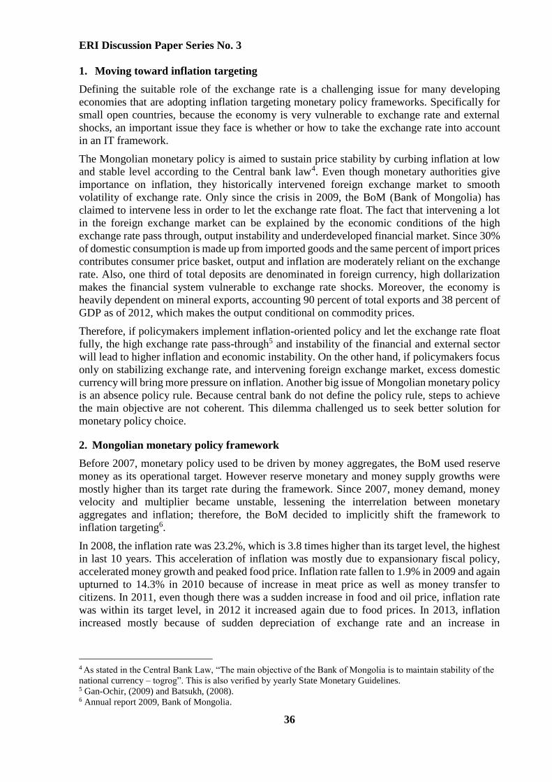
administrative prices. Summarizing achievement of inflation targeting, 2 of 6 years inflation

was lower than its target level.

TABLE 1 INFLATION TARGET

AND PERFORMANCE

Inflation

Target (%) Actual (%)

2007 5 14

2008 6 23.2

2009 9.9 1.9

2010 8 14.3

2011 9.9 9.4

2012 9.9 14.2

2013 8 12.3

Source: Monetary Policy Guidelines, Monthly bulletin of BoM

FIGURE 1: INFLATION TARGET AND PERFORMANCE

Source: Monetary Policy Guidelines, Monthly bulletin of BoM

The BoM raised a policy rate from 9.75% to 14% in 2009 in order to prevent high volatility of

domestic currency. As the economy faces crisis by the end of 2009, interest rate was decreased

gradually. Then, the BoM raised the policy rate 2times to 13.25% in 2012 to offset excess

demand from expansionary fiscal policy. In 2013, they decreased policy rate 3 times to 10.5%

as inflation pressures decline.

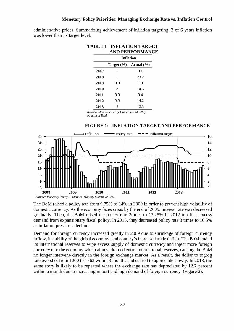
Demand for foreign currency increased greatly in 2009 due to shrinkage of foreign currency

inflow, instability of the global economy, and country’s increased trade deficit. The BoM traded

its international reserves to wipe excess supply of domestic currency and inject more foreign

currency into the economy which almost drained entire international reserves, causing the BoM

no longer intervene directly in the foreign exchange market. As a result, the dollar to togrog

rate overshot from 1200 to 1563 within 3 months and started to appreciate slowly. In 2013, the

same story is likely to be repeated where the exchange rate has depreciated by 12.7 percent

within a month due to increasing import and high demand of foreign currency. (Figure 2).

0

2

4

6

8

10

12

14

16

-5

0

5

10

15

20

25

30

35

2008 2009 2010 2011 2012 2013

Inflation Policy rate Inflation target


38

FIGURE 2: EXCHANGE RATE AND INTERNATIONAL RESERVES CHANGE

Source: www.mongolbank.mn

Here arises the question, what would be the priority of monetary policy for small open

economies like Mongolia? Should it ignore exchange rate fluctuations? Next chapter tries to

answer the question by comparing different monetary policy frameworks and research works

that were studied in this field.

3. Review of the international experiences and literature

The choosing the preferred exchange rate regime for developing economies has evolved sizably

over the past couple of decades. Mussa et al. (2000) find that developing countries have been

moving their exchange rate regimes toward greater flexibility, getting to expanding

opportunities from an increasingly integrated global economy and to changes in their own

economic situations. Moreover, the results show that, facing generally larger macroeconomic

shocks than the advanced countries, developing countries with flexible exchange rates placed

substantially greater importance on the stability of their exchange rates than did the G–3, and

significantly greater importance on average than did the other industrial countries with floating

rates. From this experience, it is clear that developing countries that maintain relatively flexible

exchange rate regimes typically use both monetary policy adjustments and official intervention

to influence the exchange rate.

How does economic performance differ across exchange rate regimes? Rogoff et al. (2003)

explored this question empirically for using the natural classification of de facto exchange rate

regimes. The findings suggest that exchange rate flexibility becomes more valuable as countries

mature in terms of their access to international capital markets and as they develop their

financial systems. Particularly for developing countries, the inflation benefit associated with

exchange rate pegs is great if it is an explicit, publicly announced policy goal.

IMF review of exchange rate regimes in 1999 suggests the following conditions are likely to

influence whether some form of pegged exchange rate regime is judged to be appropriate:

The degree of involvement with international capital markets is low;

The share of trade with the country to which it is pegged is high;

The shocks it faces are similar to those facing the country to which it pegs;

It is willing to give up monetary independence for its partner’s monetary credibility;

Its economy and financial system already extensively relies on its partners’ currency;

Because of high inherited inflation, exchange rate based stabilization is attractive;

Its fiscal policy is flexible and sustainable;

-100

-50

0

50

100

150

200

1100

1250

1400

1550

1700

1850

2008 2009 2010 2011 2012 2013

Change of International Reserves, yoy MNT/USD exchange rate, monthly average %

http://www.mongolbank.mn/


39

Its labor markets are flexible;

It has high international reserves.

On the contrary to the pegged exchange rate regime, а genuine floating exchange rate allows

more flexibility for monetary policy in times of exchange rate pressures and economic struggle.

Also, provided that the exchange rate really does move up and down in response to market

forces, businesses and financial institutions are forced to identify the risks inherent in foreign

exchange risk. Central bank independence is important to help mitigate fears that the lack of

exchange rate anchor could let loose the money-printing demon.

The fixed-to-float framework of exchange rate has been very cautious, considering a number

of challenges typically associated with fear of floating: concerns about losing a transparent

nominal anchor and policy credibility, potential exchange rate losses associated with currency

mismatches in corporate balance sheets, weaknesses in banks’ risk management practices and

lack of hedging markets and instruments to cover against exchange rate risks, underdeveloped

financial markets, and fears of worsening of external competitiveness should the currency

appreciate. Otker-Robe et al.(2007) Using six country’s experiences suggest that those that

work on mitigating risks associated with floating can achieve a smoother exit from their pegged

regimes, even when the elements supporting greater flexibility are not fully in place before the

move to greater flexibility.

4. The Role of Exchange Rate in Inflation-Targeting Emerging Economies

The exchange rate plays an important role in monetary policy for emerging economies that have

adopted inflation targeting or considering moving on IT framework. Inflation targeting

emerging economies generally have less flexible exchange rate arrangements and intervene

more frequently in the foreign exchange market. However, their sharper focus on the exchange

rate may cause some confusion about the commitment of their central banks to the inflation

target and may also complicate policy implementation.

The policy and operational role of the exchange rate within the monetary framework of

inflation-targeting emerging economies as well as emerging economies with other anchors

make the transition to inflation targeting reflects strong, uncertain, and heterogeneous exchange

rate channels for a number of reasons including high pass-through from the exchange rate to

inflation, the impact on output of exchange rate movement, balance sheet mismatches,

underdeveloped financial markets, and lower overall policy credibility(Stone et al. (2009),

Filardo et al.(2011), Calvo and Reihart (2000), Engel (2011).

Pass-through from the exchange rate to inflation: Pass-through from the exchange rate to

inflation is especially important for emerging economies, in part reflecting lower policy

credibility. Ho and McCauley (2003) comparing the experience of 12 emerging market inflation

targeting countries with six industrial country counterparts argue that emerging market

economies tend to be relatively more exposed to exchange rate fluctuations for various

structural and historical reasons. Gagnon and Ihrig (2004) propose that the anti-inflationary

actions and credibility of the monetary authority are important factors behind the reduced pass-

through of exchange rate changes to domestic inflation via evidence from a sample of 11

industrial countries that inflation-targeting (IT) exhibited a marked change in monetary

behavior in the 1990s and that pass-through declined more sharply in IT countries than

elsewhere. Frankel et al. (2005) using a new data set prices of eight narrowly defined brand

commodities, find the empirical support for significant determinants of the pass-through

coefficient include per capita incomes, bilateral distance, tariffs, country size, wages, long-term

inflation, and long-term exchange rate variability.


40

Output stability: Bahmani-Oskooee and Kutan (2008) investigated the impact of real

depreciation on output both short-run and long-run in experience of nine emerging economies.

The result shows that in short-run, real depreciation is expansionary in Belarus, Latvia, Poland,

and Slovak Republic; contractionary in Czech Republic, Estonia, Hungary, and Russia; and has

no effect in Lithuania. However, in almost none of the country, the short-run effects lasted into

the long-run. Aghion et al. (2007) offer empirical evidence that real exchange rate volatility can

have a significant impact on long-term rate of productivity growth, but the effect depends

critically on a country’s level of financial development. They find that for countries with

relatively low levels of financial development, exchange rate volatility generally reduces

growth, whereas for financially advanced countries, there is no significant effect. But the using

exchange rate to smooth output volatility can create confusion regarding the commitment to an

inflation target or objective.

Financial and External stability: Mussa et al.(2000) pointed out that prudential risks and

vulnerabilities in the banking system present challenges when moving toward a flexible-

exchange-rate arrangement. Currency mismatch is a disparity in the currencies in which assets

and liabilities are denominated. Because of, liabilities may be denominated in a foreign

currency, while assets are allocated in domestic currency, leading to compel huge losses when

there is a devaluation of the domestic currency. Currency mismatches appeared generally in

emerging economies than in developed economies as conclusion of Allen et al.(2002). Stone et

al. (2009) found that prolonged foreign exchange intervention to stabilize the exchange rate can

lead the authorities to take on a large share of currency risk, encouraging further large capital

inflows and increasing the risk of a sudden stop. There are trade-offs between using exchange

rate management to address financial and external stability concerns and using it to promote

price and output stability.

Underdeveloped financial market: Underdeveloped domestic financial markets reduce the

scope for exchange rate flexibility by amplifying exchange rate shocks and constraining policy

implementation. Developed money markets and government security markets also provide

more policy options. Weak interest rate transmission from underdeveloped money markets can

compel a leading policy role for the exchange rate. Furthermore, underdeveloped money and

security markets can raise the costs of sterilization and result in large liquidity creation from

capital inflows. The absence of developed money markets also can inhibit the adoption of

inflation targeting under which a short-term interest rate is used as the operating target.

Central bank Credibility: A high degree of overall policy credibility frees up the exchange

rate to float and enhances policy implementation and thus is necessary for the adoption of a

full-fledged inflation-targeting nominal anchor. These preconditions to inflation targeting

framework including institutional independence, a well-developed technical infrastructure,

economic structure, a healthy financial system, all inflation-targeting central bank needs a

mandate to pursue the inflation target and autonomy to set its monetary instruments accordingly

to support and motivate the commitment to low inflation. Batini et al.(2005) Find that for most

emerging economies, however, with lacking technical capabilities and central bank autonomy,

would be better off sticking with a conventional policy framework, such as an exchange rate

peg or money growth. They argue that there is not appear to be necessary for emerging market

countries to meet a stringent set of institutional, technical, and economic “preconditions” for

the successful adoption of inflation targeting. Instead, the feasibility and success of inflation

targeting appear to depend more on the authorities’ commitment and ability to plan and drive

institutional change after the introduction of inflation targeting. Lack of credibility will lead to

fear of floating, high interest rate volatility and pro-cyclical interest rate policies. Furthermore,

it may give rise to liability dollarization and limit the central bank’s ability to act as an effective


41

lender of last resort, all of which feed this fear of large exchange rate fluctuates (Calvo and

Reinhart, 2000).

Stone et al. (2009) test that policy trade-off is gauged using a small economic model to simulate

the impact of shocks on both advanced and emerging economies under different policy rules.

In general, the analysis tends to confirm the finding of earlier analysis that advanced or

financially robust economies have little to gain from including the exchange rate explicitly in

their policy reaction function, particularly in response to demand shocks. At the same time, the

analysis suggests that financially vulnerable emerging economies might benefit from including

the exchange rate in the reaction function in a limited way, but that too much emphasis on the

exchange rate is likely to be harmful. Including the exchange rate the policy reaction function

appears to help mitigate the impacts of risk premium shocks and cost-push shocks, and

especially by dampening interest rate and exchange rate volatility. Ball (1999) a similar result

in that in a closed economy, inflation targeting and Taylor rules perform well in stabilizing both

output and inflation. In an open economy, however, these policies perform poorly unless they

are modified. Specifically, if policymakers minimize a weighted sum of output and inflation

variances, their policy instrument should be an MCI based on both the interest rate and the

exchange rate.

Therefore, the establishing a more systematic, consistent, and market-based role for the

exchange rate is a key to making the transition to inflation targeting. Because of, an effective

role for the exchange rate in policy implementation under an inflation-targeting framework can

reduce conflicts between the inflation objective and other considerations. Transparency for the

role of the exchange rate with respect to policy objectives, operation procedures, and ex post

evaluation reduces the possibility of confusion about the inflation target. Low operational

transparency may lead markets question whether a change in the policy interest rate or a foreign

exchange market intervention is aimed at supporting the inflation target or only at managing

exchange rate itself.

4.1. The Role of Exchange Rate in Mongolian Economy

Mongolia is a small open economy. Therefore exchange rate volatility has considerable effect

on prices of export and import. The fluctuation of the exchange rate affects directly to these

prices and indirectly to the domestic goods and services through imported inputs.

Batsukh (2008) analyzed the cycle and trend correlation between Mongolian CPI and nominal

exchange rate of togrog against U.S dollar. According to the result, cycle and trend coefficients

of exchange rate to CPI are 0.49 and 0.89 respectively with a lagged effect. This result was also

proven by Gan-Ochir (2009) where he measured the exchange rate pass through to consumer

price inflation in Mongolia, analyzing monthly data from a recursive VAR model. The

accumulated impact of exchange rate shock on consumer prices was 10 percent by the end of

the fifth month after the depreciation shock introduced, and 55 percent by the end of the ninth

month, showing high pass through of exchange rate of consumer prices. An early study by

Davaajargal (2005) and Khulan (2005)also found the lagged effect of exchange rate on

consumer price starting from the third month intense till the sixth month after exchange rate

shock. In recent years, studies such as Gan-Ochir (2011), Avralt-Od and Davaadalai (2010)

resulted similar results of high pass through of exchange rate to inflation in Mongolia using

SVAR and SBVAR models.

Narantuya et al. (2009) evaluated the impact of the global financial and economic crisis in the

Mongolian economy for four consequent quarters of 2009.They concluded that the impact of

the global financial and economic crisis affected domestic output straightforwardly through the

drop in foreign trade since there were no room for counter-cyclical monetary or fiscal policy.


42

Furthermore, they marked that monetary policy measures against rapidly increased inflation

resulted even more bust in the real sector.

Tuvshintugs (2009) argued that the BoM’s monetary policy decisions before the crisis were not

independent from the government. Even though the BoM was to conduct monetary policy to

achieve the goal of low stable inflation, political pressure from the government or parliament

made them to choose a monetary policy which supports an economic growth and employment

resulting even worse macroeconomic circumstances. According to his view, the BoM does not

have an enough power to oppose the parliament and its independence is inferior regarding the

legal environment.

Recently, Avralt-Od et al.(2011) Examined the medium term outlook of the Mongolian

economy using the DSGE model. They concluded that less involvement of central bank in the

foreign exchange market and increasing income in mining sector would lead higher demand

and appreciation of real exchange rate in the economy. Even though real exchange rate

appreciation might decrease the production of tradable sector, the government investment

would accumulate both social and private capital resulting stable economic growth. They

warned that any attempt to decrease the real exchange rate appreciation may cause crowding

out effect on private investment and slow down economic growth in the medium term.

In May 2011, a staff team of the IMF assessed research on Mongolian financial stability. They

concluded that Mongolian financial stability has been re-established after the banking crisis of

2008-09,however the banking system is heavily exposed to several risks including exchange

rate risks due to maturity mismatches and unhedged foreign currency lending. From their

findings of the assessment, foreign currency lending has increased, and lending to unhedged

borrowers rendered the system vulnerable to foreign exchange induced credit risk; the current

level of dollarization exposed the Mongolian financial system to risk.

However, above mentioned researchers analyzed the effect of exchange rate in the economy,

no research was done to compare the monetary policy rules using a DSGE model which opened

us a gap in the field to study.

5. A small open economy model

We used small open economy Dynamic Stochastic General Equilibrium (DSGE) model with

natural resource sector based on Roger, Rest repo & Garcia (2009) to evaluate the performances

of alternative IT approaches. Total output consists of two types of goods. The first one is a

composite good produced by monopolistically competitive firms both for domestic

consumption and export. The second good is a natural resource commodity for export. The

economy consists of the following agents: two types of households, some participating in asset

markets and others not; natural resource producing firms, composite good producer, and a

central bank in charge of monetary policy. The development of each agents movements are

described in Appendix 1.

5.1. Log-linearised equations of the model

The empirical analysis employs a log-linear approximation of the models optimality conditions

around a non-stochastic steady state. We here shown the key structural equations that emerge

from the analysis. All variables are properly interpreted as log deviations from their respective

steady state values.

𝐷𝑜𝑚𝑒𝑠𝑡𝑖𝑐 𝑝𝑟𝑜𝑑𝑢𝑐𝑡𝑖𝑜𝑛: �̂�𝑡𝑑 = �̂�𝑡[𝛼

𝜂 + (1 − 𝛼)𝜂] + [𝛼𝜂 ∙ 𝑖�̂�𝑡 + (1 − 𝛼)𝜂 ∙ 𝑙𝑡]; ( 1 )

𝑀𝑎𝑟𝑔𝑖𝑛𝑎𝑙 𝑐𝑜𝑠𝑡: 𝑚�̂�𝑡𝑟 = [[1 − 𝛼]𝜂 ∙ [�̂�𝑡 − �̂�𝑡] + [𝛼]𝜂 ∙ �̂�𝑡] − �̂�𝑡 ∙ ([1 − 𝛼]𝜂 + [𝛼]𝜂); ( 2 )


43

𝐸𝑥𝑝𝑜𝑟𝑡 𝑑𝑒𝑚𝑎𝑛𝑑: 𝑥𝑡𝑑 = 𝛾 ∙ 𝑥𝑡−1

𝑑 + (1 − 𝛾)[𝜏�̂�𝑡 + �̂�𝑡∗] ( 3 )

𝑅𝑖𝑠𝑘 𝑝𝑟𝑒𝑚𝑖𝑢𝑚: �̂�𝑡 = 𝜙0(�̂�𝑡+1∗ − �̂�𝑡) − 𝜙1((𝜏 − 1)�̂�𝑡 + �̂�𝑡

∗) + 𝜙2(𝑖�̂�𝑡) + 𝜙3(�̂�𝑡) ( 4 )

𝑃ℎ𝑖𝑙𝑙𝑖𝑝𝑠 𝑐𝑢𝑟𝑣𝑒: �̂�𝑡 = (𝛽 1 + 𝛽𝜇⁄ )�̂�𝑡+1 + (𝜇 1 + 𝛽𝜇⁄ )�̂�𝑡−1 + (𝜍 1 + 𝛽𝜇⁄ )�̂�𝑐𝑡𝑟 ( 5 )

𝑅𝑒𝑎𝑙 𝑒𝑥𝑐ℎ𝑎𝑛𝑔𝑒 𝑟𝑎𝑡𝑒:

�̂�𝑡 = (1 − 𝜙𝑠)�̂�𝑡+1 + 𝜙𝑠�̂�𝑡−1 − (𝑖̂𝑡 − �̂�𝑡+1) + (𝑖̂𝑡∗ − �̂�𝑡+1

∗ ) + �̂�𝑡 ( 6 )

𝑷𝒐𝒍𝒊𝒄𝒚 𝒓𝒖𝒍𝒆𝒔

𝑃𝑙𝑎𝑖𝑛 𝑣𝑎𝑛𝑖𝑙𝑙𝑎 𝐼𝑇: 𝑖�̂� = 𝜔 ∙ 𝑖�̂�−1 + (1 − 𝜔)[𝛿�̂�𝑡 + 𝜚�̂�𝑡] + 𝜈𝑡 ( 7 )

𝑂𝑝𝑒𝑛 𝑒𝑐𝑜𝑛𝑜𝑚𝑦 𝐼𝑇: 𝑖̂𝑡 = 𝜔 ∙ 𝑖̂𝑡−1 + (1 − 𝜔)[𝛿�̂�𝑡 + 𝜚�̂�𝑡 + 𝜒(�̂�𝑡 − 𝜖 ∙ �̂�𝑡−1)] + 𝑣𝑡 ( 8 )

𝐸𝑥𝑐ℎ𝑎𝑛𝑔𝑒 𝑟𝑎𝑡𝑒 𝑏𝑎𝑛𝑑 𝐼𝑇: 𝑖�̂� = 𝜔 ∙ 𝑖�̂�−1 + (1 − 𝜔)[𝛿�̂�𝑡 + 𝜚�̂�𝑡 + (𝜒 + 𝜓) ∗ (�̂�𝑡 − 𝜖 ∙ �̂�𝑡−1)] + 𝑣𝑡

( 9 )

𝐸𝑥𝑐ℎ𝑎𝑛𝑔𝑒 𝑟𝑎𝑡𝑒 𝑏𝑎𝑠𝑒𝑑 𝐼𝑇: �̂�𝑡 = 𝜌𝑞�̂�𝑡−1 + (1 − 𝜌𝑞)[𝛿�̂�𝑡 + 𝜚�̂�𝑡] + 𝑣𝑡 ( 10 )

where �̂�𝑡𝑑- total production, �̂�𝑡- total factor productivity, 𝑖�̂�𝑡- imported intermediate input, 𝑙𝑡-

labor input, 𝑚�̂�𝑡𝑟-real marginal cost of production, �̂�𝑡- nominal wage rate per unit of work

supplied, �̂�𝑡- price level, �̂�𝑡- real exchange rate, �̂�𝑡𝑑- export demand, �̂�𝑡

∗- foreign real income,

�̂�𝑡- aggregate inflation rate, 𝑖̂𝑡∗- foreign nominal interest rate, �̂�𝑡+1

∗ -expected foreign inflation

rate, �̂�𝑡- risk premium7, �̂�𝑡+1 ∗ - projected external debt in period 𝑡 + 1.

𝑖�̂� ≡ 𝑖𝑡 − (�̅� + 𝜋𝑇)- Deviation of policy target interest rate from its long-run steady-state value.

�̂�𝑡 ≡ 𝜋𝑡𝑓

− 𝜋𝑇- Deviation of inflation forecast from the inflation target. �̂�𝑡 ≡ 𝑦𝑡 − �̅�𝑡- Deviation of real output from the estimated level of potential output.

Foreign economy is specified as the closed economy variant of the model as described in Mona

celli (2005). Because the foreign economy is exogenous to the domestic economy, we assumed

that the paths of (�̂�𝑡∗,�̂�𝑡

∗,𝑖̂𝑡∗) are determined by a vector autoregressive processes of order one.

6. Methodology

We calibrated the parameters of the model and we used Dynare toolbox in Matlab software to

solve a log-linearized model and run policy simulations. The main variables are output gap,

inflation, exchange rate and interest rate.

6.1. Calibration

The model is calibrated based on literature, values taken from findings of different studies and

country specific indicators. Parameters of monetary policy rule are changeable depending on

which policy decision to make.

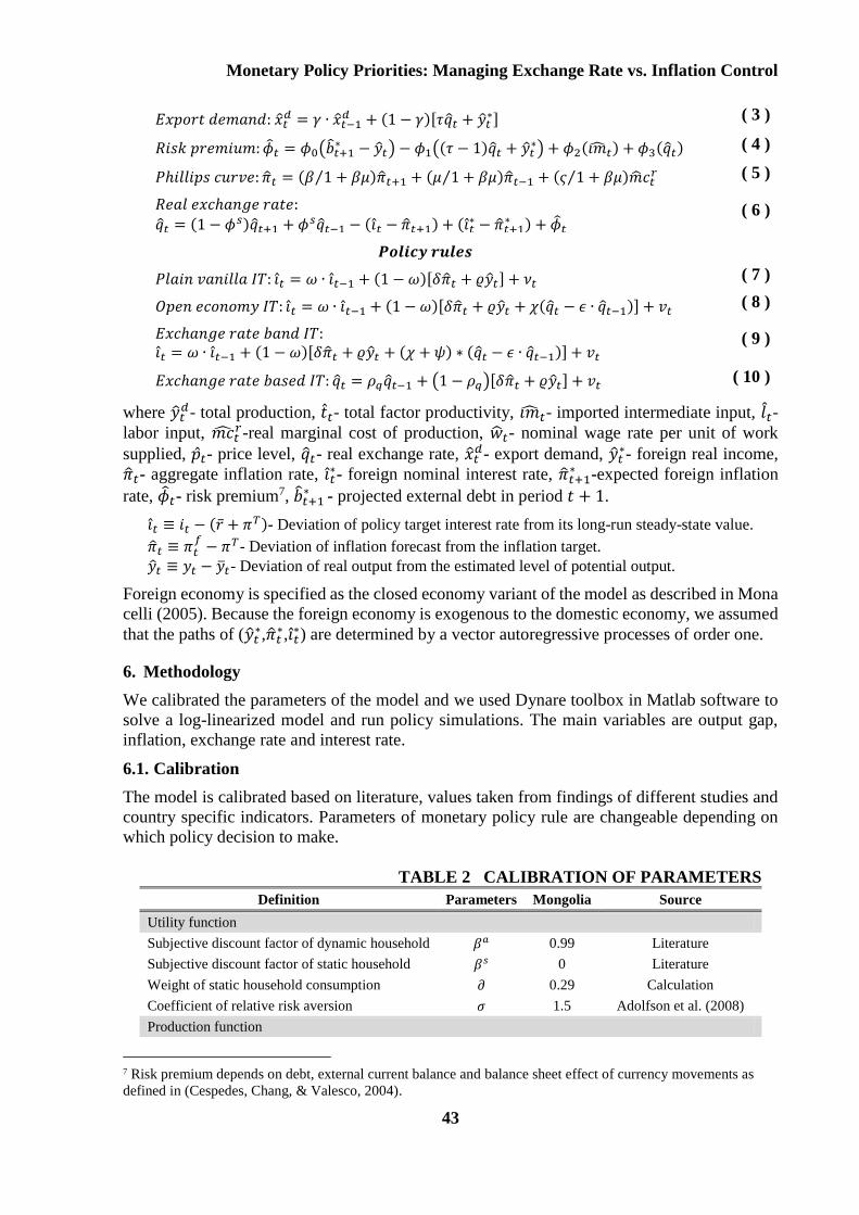
TABLE 2 CALIBRATION OF PARAMETERS

Definition Parameters Mongolia Source

Utility function

Subjective discount factor of dynamic household 𝛽𝑎 0.99 Literature

Subjective discount factor of static household 𝛽𝑠 0 Literature

Weight of static household consumption 𝜕 0.29 Calculation

Coefficient of relative risk aversion 𝜎 1.5 Adolfson et al. (2008)

Production function

7 Risk premium depends on debt, external current balance and balance sheet effect of currency movements as

defined in (Cespedes, Chang, & Valesco, 2004).


44

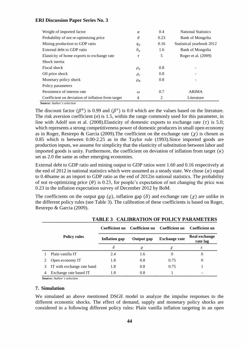
Weight of imported factor 𝛼 0.4 National Statistics

Probability of not re-optimizing price 𝜗 0.23 Bank of Mongolia

Mining production to GDP ratio 𝑞𝑦 0.16 Statistical yearbook 2012

External debt to GDP ratio 𝑏𝑦 1.6 Bank of Mongolia

Elasticity of home exports to exchange rate 𝜏 5 Roger et al. (2009)

Shock inertia

Fiscal shock 𝜌𝑦 0.8 -

Oil price shock 𝜌𝑐 0.8 -

Monetary policy shock 𝜌𝑅 0.8 -

Policy parameters

Persistence of interest rate 𝜔 0.7 ARIMA

Coefficient on deviation of inflation from target 𝑘 2 Literature

Source: Author’s selection

The discount factor (𝛽𝑎) is 0.99 and (𝛽𝑠) is 0.0 which are the values based on the literature.

The risk aversion coefficient (σ) is 1.5, within the range commonly used for this parameter, in

line with Adolf son et al. (2008).Elasticity of domestic exports to exchange rate (𝜏) is 5.0;

which represents a strong competitiveness power of domestic producers in small open economy

as in Roger, Restrepo & Garcia (2009).The coefficient on the exchange rate (𝜒) is chosen as

0.85 which is between 0.00-2.25 as in the Taylor rule (1993).Since imported goods are

production inputs, we assume for simplicity that the elasticity of substitution between labor and

imported goods is unity. Furthermore, the coefficient on deviation of inflation from target (𝜅)

set as 2.0 the same as other emerging economies.

External debt to GDP ratio and mining output to GDP ratios were 1.60 and 0.16 respectively at

the end of 2012 in national statistics which were assumed as a steady state. We chose (𝛼) equal

to 0.40same as an import to GDP ratio as the end of 2012in national statistics. The probability

of not re-optimizing price (𝜃) is 0.23, for people’s expectation of not changing the price was

0.23 in the inflation expectation survey of December 2012 by BoM.

The coefficients on the output gap (𝜚), inflation gap (𝛿) and exchange rate (𝜒) are unlike in

the different policy rules (see Table 3). The calibration of these coefficients is based on Roger,

Restrepo & Garcia (2009).

TABLE 3 CALIBRATION OF POLICY PARAMETERS

Policy rules

Coefficient on Coefficient on Coefficient on Coefficient on

Inflation gap Output gap Exchange rate Real exchange

rate lag

𝛿 𝜚 𝜒 휀

1 Plain vanilla IT 2.4 1.6 0 0

2 Open economy IT 1.8 0.8 0.75 0

3 IT with exchange rate band 1.8 0.8 0.75 1

4 Exchange rate based IT 1.8 0.8 1 -


7. Simulation

We simulated an above mentioned DSGE model to analyze the impulse responses to the

different economic shocks. The effect of demand, supply and monetary policy shocks are

considered in a following different policy rules: Plain vanilla inflation targeting in an open


45

economy, open economy inflation targeting, inflation targeting with exchange rate band and

exchange rate-based inflation targeting. The radars showed the highest variability of

observables from its steady state value since shocks were introduced in different policy rules.

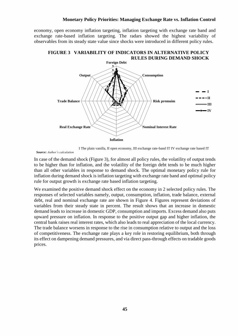
FIGURE 3 VARIABILITY OF INDICATORS IN ALTERNATIVE POLICY

RULES DURING DEMAND SHOCK

I The plain vanilla, II open economy, III exchange rate-band IT IV exchange rate based IT Source: Author’s calculation

In case of the demand shock (Figure 3), for almost all policy rules, the volatility of output tends

to be higher than for inflation, and the volatility of the foreign debt tends to be much higher

than all other variables in response to demand shock. The optimal monetary policy rule for

inflation during demand shock is inflation targeting with exchange rate band and optimal policy

rule for output growth is exchange rate based inflation targeting.

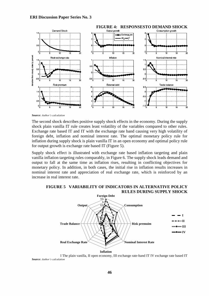
We examined the positive demand shock effect on the economy in 2 selected policy rules. The

responses of selected variables namely, output, consumption, inflation, trade balance, external

debt, real and nominal exchange rate are shown in Figure 4. Figures represent deviations of

variables from their steady state in percent. The result shows that an increase in domestic

demand leads to increase in domestic GDP, consumption and imports. Excess demand also puts

upward pressure on inflation. In response to the positive output gap and higher inflation, the

central bank raises real interest rates, which also leads to real appreciation of the local currency.

The trade balance worsens in response to the rise in consumption relative to output and the loss

of competitiveness. The exchange rate plays a key role in restoring equilibrium, both through

its effect on dampening demand pressures, and via direct pass-through effects on tradable goods

prices.

0

1

2

3

4

5

6

7

8

9

Foreign Debt

Consumption

Risk premuim

Nominal Interest Rate

Inflation

Real Exchange Rate

Trade Balance

Output

I

II

III

IV


46

FIGURE 4: RESPONSESTO DEMAND SHOCK

Source: Author’s calculation

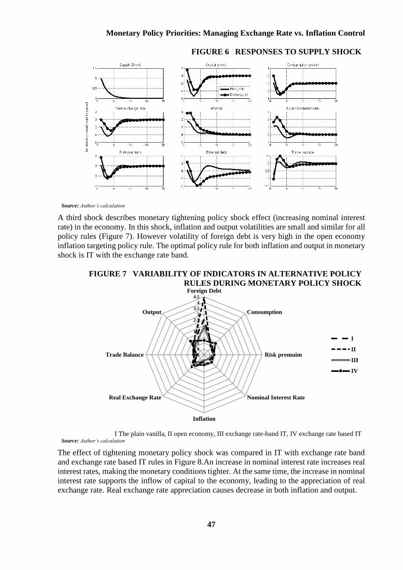
The second shock describes positive supply shock effects in the economy. During the supply

shock plain vanilla IT rule creates least volatility of the variables compared to other rules.

Exchange rate based IT and IT with the exchange rate band causing very high volatility of

foreign debt, inflation and nominal interest rate. The optimal monetary policy rule for

inflation during supply shock is plain vanilla IT in an open economy and optimal policy rule

for output growth is exchange rate based IT (Figure 5).

Supply shock effect is illustrated with exchange rate based inflation targeting and plain

vanilla inflation targeting rules comparably, in Figure 6. The supply shock leads demand and

output to fall at the same time as inflation rises, resulting in conflicting objectives for

monetary policy. In addition, in both cases, the initial rise in inflation results increases in

nominal interest rate and appreciation of real exchange rate, which is reinforced by an

increase in real interest rate.


RULES DURING SUPPLY SHOCK

I The plain vanilla, II open economy, III exchange rate-band IT IV exchange rate based IT Source: Author’s calculation

-0.5

0

0.5

1

1.5

2

2.5

3

3.5Foreign Debt

Consumption

Risk premuim


Inflation

Real Exchange Rate

Trade Balance

Output

I

II

III

IV


47

FIGURE 6 RESPONSES TO SUPPLY SHOCK


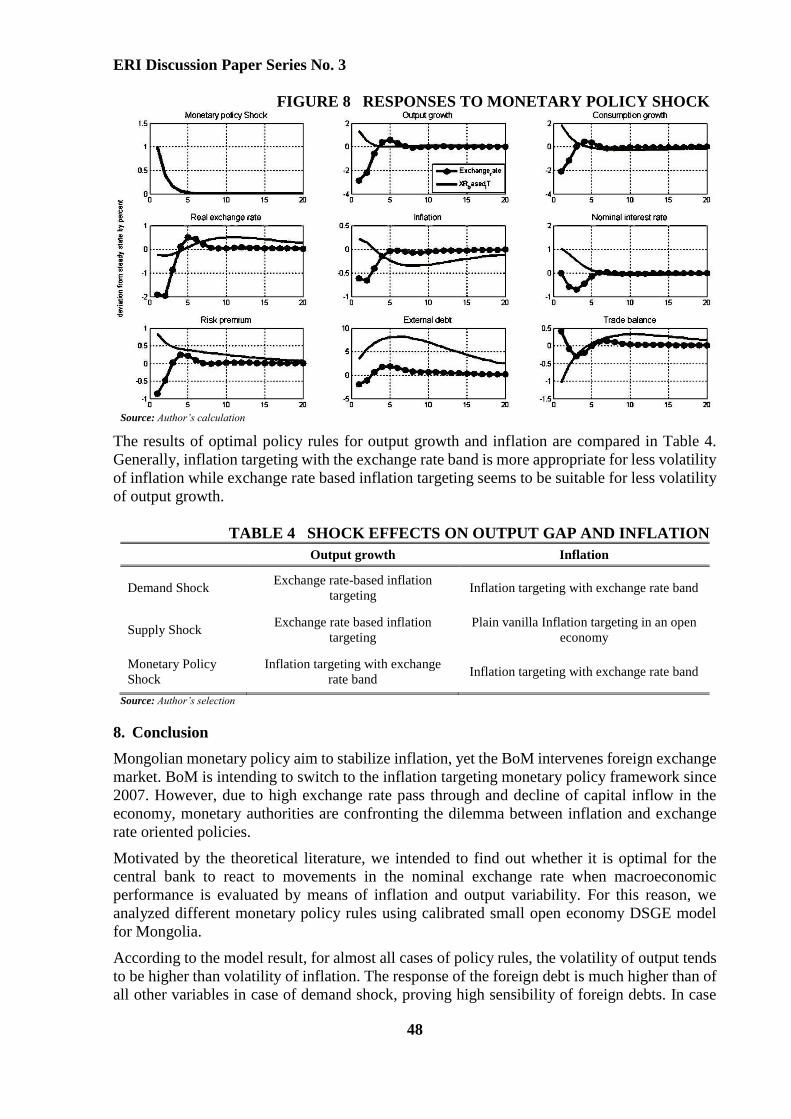
A third shock describes monetary tightening policy shock effect (increasing nominal interest

rate) in the economy. In this shock, inflation and output volatilities are small and similar for all

policy rules (Figure 7). However volatility of foreign debt is very high in the open economy

inflation targeting policy rule. The optimal policy rule for both inflation and output in monetary

shock is IT with the exchange rate band.


RULES DURING MONETARY POLICY SHOCK

I The plain vanilla, II open economy, III exchange rate-band IT, IV exchange rate based IT Source: Author’s calculation

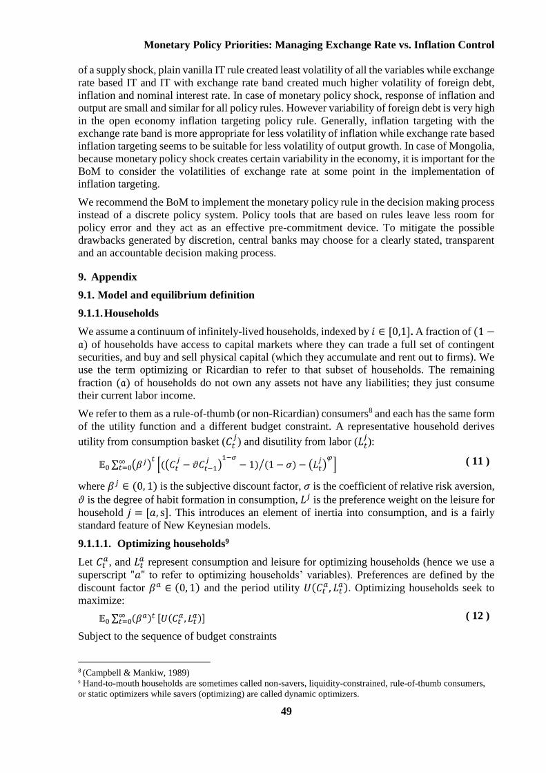
The effect of tightening monetary policy shock was compared in IT with exchange rate band

and exchange rate based IT rules in Figure 8.An increase in nominal interest rate increases real

interest rates, making the monetary conditions tighter. At the same time, the increase in nominal

interest rate supports the inflow of capital to the economy, leading to the appreciation of real

exchange rate. Real exchange rate appreciation causes decrease in both inflation and output.

-0.5

0

0.5

1

1.5

2

2.5

3

3.5

4

4.5

Foreign Debt

Consumption

Risk premuim


Inflation

Real Exchange Rate

Trade Balance

Output

I

II

III

IV


48

FIGURE 8 RESPONSES TO MONETARY POLICY SHOCK


The results of optimal policy rules for output growth and inflation are compared in Table 4.

Generally, inflation targeting with the exchange rate band is more appropriate for less volatility

of inflation while exchange rate based inflation targeting seems to be suitable for less volatility

of output growth.

TABLE 4 SHOCK EFFECTS ON OUTPUT GAP AND INFLATION

Output growth Inflation

Demand Shock Exchange rate-based inflation

targeting Inflation targeting with exchange rate band

Supply Shock Exchange rate based inflation

targeting

Plain vanilla Inflation targeting in an open

economy

Monetary Policy

Shock

Inflation targeting with exchange

rate band Inflation targeting with exchange rate band


8. Conclusion

Mongolian monetary policy aim to stabilize inflation, yet the BoM intervenes foreign exchange

market. BoM is intending to switch to the inflation targeting monetary policy framework since

2007. However, due to high exchange rate pass through and decline of capital inflow in the

economy, monetary authorities are confronting the dilemma between inflation and exchange

rate oriented policies.

Motivated by the theoretical literature, we intended to find out whether it is optimal for the

central bank to react to movements in the nominal exchange rate when macroeconomic

performance is evaluated by means of inflation and output variability. For this reason, we

analyzed different monetary policy rules using calibrated small open economy DSGE model

for Mongolia.

According to the model result, for almost all cases of policy rules, the volatility of output tends

to be higher than volatility of inflation. The response of the foreign debt is much higher than of

all other variables in case of demand shock, proving high sensibility of foreign debts. In case


49

of a supply shock, plain vanilla IT rule created least volatility of all the variables while exchange

rate based IT and IT with exchange rate band created much higher volatility of foreign debt,

inflation and nominal interest rate. In case of monetary policy shock, response of inflation and

output are small and similar for all policy rules. However variability of foreign debt is very high

in the open economy inflation targeting policy rule. Generally, inflation targeting with the

exchange rate band is more appropriate for less volatility of inflation while exchange rate based

inflation targeting seems to be suitable for less volatility of output growth. In case of Mongolia,

because monetary policy shock creates certain variability in the economy, it is important for the

BoM to consider the volatilities of exchange rate at some point in the implementation of

inflation targeting.

We recommend the BoM to implement the monetary policy rule in the decision making process

instead of a discrete policy system. Policy tools that are based on rules leave less room for

policy error and they act as an effective pre-commitment device. To mitigate the possible

drawbacks generated by discretion, central banks may choose for a clearly stated, transparent

and an accountable decision making process.

9. Appendix

9.1. Model and equilibrium definition

9.1.1. Households

We assume a continuum of infinitely-lived households, indexed by 𝑖 ∈ [0,1]. A fraction of (1 −𝔞) of households have access to capital markets where they can trade a full set of contingent

securities, and buy and sell physical capital (which they accumulate and rent out to firms). We

use the term optimizing or Ricardian to refer to that subset of households. The remaining

fraction (𝔞) of households do not own any assets not have any liabilities; they just consume

their current labor income.

We refer to them as a rule-of-thumb (or non-Ricardian) consumers8 and each has the same form

of the utility function and a different budget constraint. A representative household derives

utility from consumption basket (𝐶𝑡𝑗) and disutility from labor (𝐿𝑡

𝑗):

𝔼0 ∑ (𝛽𝑗)𝑡∞

𝑡=0 [((𝐶𝑡𝑗− 𝜗𝐶𝑡−1

𝑗)1−𝜎

− 1) (1 − 𝜎)⁄ − (𝐿𝑡𝑗)𝜑] ( 11 )

where 𝛽𝑗 ∈ (0, 1) is the subjective discount factor, 𝜎 is the coefficient of relative risk aversion,

𝜗 is the degree of habit formation in consumption, 𝐿𝑗 is the preference weight on the leisure for

household 𝑗 = [𝑎, s]. This introduces an element of inertia into consumption, and is a fairly

standard feature of New Keynesian models.

9.1.1.1. Optimizing households9

Let 𝐶𝑡𝑎, and 𝐿𝑡

𝑎 represent consumption and leisure for optimizing households (hence we use a

superscript "𝑎" to refer to optimizing households’ variables). Preferences are defined by the

discount factor 𝛽𝑎 ∈ (0, 1) and the period utility 𝑈(𝐶𝑡𝑎, 𝐿𝑡

𝑎). Optimizing households seek to

maximize:

𝔼0 ∑ (𝛽𝑎)𝑡∞𝑡=0 [𝑈(𝐶𝑡

𝑎 , 𝐿𝑡𝑎)] ( 12 )

Subject to the sequence of budget constraints

8 (Campbell & Mankiw, 1989) 9 Hand-to-mouth households are sometimes called non-savers, liquidity-constrained, rule-of-thumb consumers,

or static optimizers while savers (optimizing) are called dynamic optimizers.


50

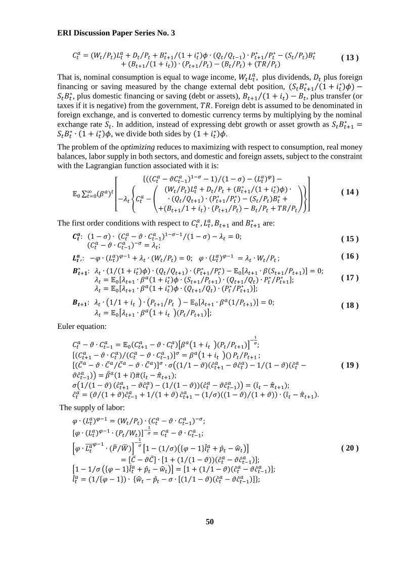
𝐶𝑡𝑎 = (𝑊𝑡 𝑃𝑡⁄ )𝐿𝑡

𝑎 + 𝐷𝑡 𝑃𝑡⁄ + 𝐵𝑡+1∗ (1 + 𝑖𝑡

∗)𝜙⁄ ∙ (𝑄𝑡 𝑄𝑡−1⁄ ) ∙ 𝑃𝑡+1∗ 𝑃𝑡

∗⁄ − (𝑆𝑡 𝑃𝑡⁄ )𝐵𝑡∗

+ (𝐵𝑡+1 (1 + 𝑖𝑡)⁄ ) ∙ (𝑃𝑡+1 𝑃𝑡⁄ ) − (𝐵𝑡 𝑃𝑡⁄ ) + (𝑇𝑅 𝑃𝑡⁄ ) ( 13 )

That is, nominal consumption is equal to wage income, 𝑊𝑡𝐿𝑡𝑎, plus dividends, 𝐷𝑡 plus foreign

financing or saving measured by the change external debt position, (𝑆𝑡𝐵𝑡+1∗ (1 + 𝑖𝑡

∗)𝜙⁄ ) −𝑆𝑡𝐵𝑡

∗, plus domestic financing or saving (debt or assets), 𝐵𝑡+1 (1 + 𝑖𝑡)⁄ − 𝐵𝑡, plus transfer (or

taxes if it is negative) from the government, 𝑇𝑅. Foreign debt is assumed to be denominated in

foreign exchange, and is converted to domestic currency terms by multiplying by the nominal

exchange rate 𝑆𝑡. In addition, instead of expressing debt growth or asset growth as 𝑆𝑡𝐵𝑡+1∗ =

𝑆𝑡𝐵𝑡∗ ∙ (1 + 𝑖𝑡

∗)𝜙, we divide both sides by (1 + 𝑖𝑡∗)𝜙.

The problem of the optimizing reduces to maximizing with respect to consumption, real money

balances, labor supply in both sectors, and domestic and foreign assets, subject to the constraint

with the Lagrangian function associated with it is:

𝔼0 ∑ (𝛽𝑎)𝑡∞𝑡=0

[

{((𝐶𝑡𝑎 − 𝜗𝐶𝑡−1

𝑎 )1−𝜎 − 1) (1 − 𝜎)⁄ − (𝐿𝑡𝑎)𝜑} −

−𝜆𝑡 {𝐶𝑡𝑎 − (

(𝑊𝑡 𝑃𝑡⁄ )𝐿𝑡𝑎 + 𝐷𝑡 𝑃𝑡⁄ + (𝐵𝑡+1

∗ (1 + 𝑖𝑡∗)𝜙⁄ ) ∙

∙ (𝑄𝑡 𝑄𝑡+1⁄ ) ∙ (𝑃𝑡+1∗ 𝑃𝑡

∗⁄ ) − (𝑆𝑡 𝑃𝑡⁄ )𝐵𝑡∗ +

+(𝐵𝑡+1 1 + 𝑖𝑡⁄ ) ∙ (𝑃𝑡+1 𝑃𝑡⁄ ) − 𝐵𝑡 𝑃𝑡⁄ + 𝑇𝑅 𝑃𝑡⁄)}

]

( 14 )

The first order conditions with respect to 𝐶𝑡𝑎 , 𝐿𝑡

𝑎, 𝐵𝑡+1 and 𝐵𝑡+1∗ are:

𝑪𝒕𝒂: (1 − 𝜎) ∙ (𝐶𝑡

𝑎 − 𝜗 ∙ 𝐶𝑡−1𝑎 )1−𝜎−1 (1 − 𝜎⁄ ) − 𝜆𝑡 = 0;

(𝐶𝑡𝑎 − 𝜗 ∙ 𝐶𝑡−1

𝑎 )−𝜎 = 𝜆𝑡; ( 15 )

𝑳𝒕𝒂,: −𝜑 ∙ (𝐿𝑡

𝑎)𝜑−1 + 𝜆𝑡 ∙ (𝑊𝑡 𝑃𝑡)⁄ = 0; 𝜑 ∙ (𝐿𝑡𝑎)𝜑−1 = 𝜆𝑡 ∙ 𝑊𝑡 𝑃𝑡⁄ ; ( 16 )

𝑩𝒕+𝟏∗ : 𝜆𝑡 ∙ (1 (1 + 𝑖𝑡

∗)𝜙⁄ ) ∙ (𝑄𝑡 𝑄𝑡+1⁄ ) ∙ (𝑃𝑡+1∗ 𝑃𝑡

∗⁄ ) − 𝔼0[𝜆𝑡+1 ∙ 𝛽(𝑆𝑡+1 𝑃𝑡+1⁄ )] = 0; 𝜆𝑡 = 𝔼0[𝜆𝑡+1 ∙ 𝛽𝑎(1 + 𝑖𝑡

∗)𝜙 ∙ (𝑆𝑡+1 𝑃𝑡+1⁄ ) ∙ (𝑄𝑡+1 𝑄𝑡⁄ ) ∙ 𝑃𝑡∗ 𝑃𝑡+1

∗⁄ ]; 𝜆𝑡 = 𝔼0[𝜆𝑡+1 ∙ 𝛽𝑎(1 + 𝑖𝑡

∗)𝜙 ∙ (𝑄𝑡+1 𝑄𝑡⁄ ) ∙ (𝑃𝑡∗ 𝑃𝑡+1

∗⁄ )];

( 17 )

𝑩𝒕+𝟏: 𝜆𝑡 ∙ (1 1 + 𝑖𝑡⁄ ) ∙ (𝑃𝑡+1 𝑃𝑡⁄ ) − 𝔼0[𝜆𝑡+1 ∙ 𝛽𝑎(1 𝑃𝑡+1⁄ )] = 0;

𝜆𝑡 = 𝔼0[𝜆𝑡+1 ∙ 𝛽𝑎(1 + 𝑖𝑡 )(𝑃𝑡 𝑃𝑡+1⁄ )]; ( 18 )

Euler equation:

𝐶𝑡𝑎 − 𝜗 ∙ 𝐶𝑡−1

𝑎 = 𝔼0(𝐶𝑡+1𝑎 − 𝜗 ∙ 𝐶𝑡

𝑎)[𝛽𝑎(1 + 𝑖𝑡 )(𝑃𝑡 𝑃𝑡+1⁄ )]−

1

𝜎;

[(𝐶𝑡+1𝑎 − 𝜗 ∙ 𝐶𝑡

𝑎) (𝐶𝑡𝑎 − 𝜗 ∙ 𝐶𝑡−1

𝑎 )⁄ ]𝜎 = 𝛽𝑎(1 + 𝑖𝑡 )()𝑃𝑡 𝑃𝑡+1⁄ ; [(𝐶̅𝑎 − 𝜗 ∙ 𝐶̅𝑎 𝐶̅𝑎 − 𝜗 ∙ 𝐶̅𝑎⁄ )]𝜎 ∙ 𝜎((1 1 − 𝜗⁄ )(�̂�𝑡+1

𝑎 − 𝜗�̂�𝑡𝑎) − 1 (1 − 𝜗⁄ )(�̂�𝑡

𝑎 −

𝜗�̂�𝑡−1𝑎 )) = �̅�𝑎(1 + 𝑖)̅�̅�(𝑖�̂� − �̂�𝑡+1);

𝜎(1 (1 − 𝜗)⁄ (�̂�𝑡+1𝑎 − 𝜗�̂�𝑡

𝑎) − (1 (1 − 𝜗)⁄ )(�̂�𝑡𝑎 − 𝜗�̂�𝑡−1

𝑎 )) = (𝑖̂𝑡 − �̂�𝑡+1); �̂�𝑡

𝑎 = (𝜗 (1 + 𝜗⁄ )�̂�𝑡−1𝑎 + 1 (1 + 𝜗)⁄ �̂�𝑡+1

𝑎 − (1 𝜎⁄ )((1 − 𝜗) (1 + 𝜗)⁄ ) ∙ (𝑖�̂� − �̂�𝑡+1).

( 19 )

The supply of labor:

𝜑 ∙ (𝐿𝑡𝑎)𝜑−1 = (𝑊𝑡 𝑃𝑡⁄ ) ∙ (𝐶𝑡

𝑎 − 𝜗 ∙ 𝐶𝑡−1𝑎 )−𝜎;

[𝜑 ∙ (𝐿𝑡𝑎)𝜑−1 ∙ (𝑃𝑡 𝑊𝑡⁄ )]−

1

𝜎 = 𝐶𝑡𝑎 − 𝜗 ∙ 𝐶𝑡−1

𝑎 ;

[𝜑 ∙ 𝐿𝑡𝑎̅̅ ̅𝜑−1

∙ (�̅� �̅�⁄ )]−

1

𝜎[1 − (1 𝜎⁄ )({𝜑 − 1}𝑙𝑡

𝑎 + �̂�𝑡 − �̂�𝑡)]

= [𝐶̅ − 𝜗𝐶̅] ∙ [1 + (1 (1 − 𝜗)⁄ )(�̂�𝑡𝑎 − 𝜗�̂�𝑡−1

𝑎 )]; [1 − 1 𝜎⁄ ({𝜑 − 1}𝑙𝑡

𝑎 + �̂�𝑡 − �̂�𝑡)] = [1 + (1 1 − 𝜗⁄ )(�̂�𝑡𝑎 − 𝜗�̂�𝑡−1

𝑎 )];

𝑙𝑡𝑎 = (1 {𝜑 − 1}⁄ ) ∙ {�̂�𝑡 − �̂�𝑡 − 𝜎 ∙ [(1 1 − 𝜗⁄ )(�̂�𝑡

𝑎 − 𝜗�̂�𝑡−1𝑎 )]};

( 20 )


51

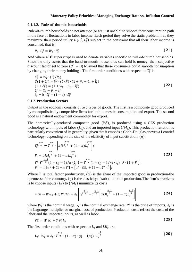
9.1.1.2. Rule-of-thumbs households

Rule-of-thumb households do not attempt (or are just unable) to smooth their consumption path

in the face of fluctuations in labor income. Each period they solve the static problem, i.e., they

maximize their period utility 𝑈(𝐶𝑡𝑠, 𝐿𝑡

𝑠) subject to the constraint that all their labor income is

consumed, that is:

𝑃𝑡 ∙ 𝐶𝑡𝑠 = 𝑊𝑡 ∙ 𝐿𝑡

𝑠 ( 21 )

And where a"𝒔" superscript is used to denote variables specific to rule-of-thumb households.

Since the only assets that the hand-to-mouth households can hold is money, their subjective

discount factor set to zero (𝛽𝑠 = 0) to avoid that these consumers could smooth consumption

by changing their money holdings. The first order conditions with respect to 𝐶𝑡𝑠 is:

𝐶𝑡𝑠 = 𝑊𝑡 ∙ (𝐿𝑡

𝑠 𝑃𝑡)⁄ 𝐶̅(1 + �̂�𝑡

𝑠) = �̅� ∙ (�̅� �̅�⁄ ) ∙ (1 + �̂�𝑡 − �̂�𝑡 + 𝑙𝑡𝑠)

(1 + �̂�𝑡𝑠) = (1 + �̂�𝑡 − �̂�𝑡 + 𝑙𝑡

𝑠) �̂�𝑡

𝑠 = �̂�𝑡 − �̂�𝑡 + 𝑙𝑡𝑠

�̂�𝑡 = 𝔡 ∙ �̂�𝑡𝑠 + (1 − 𝔡) ∙ �̂�𝑡

𝑎

( 22 )

9.1.2. Production Sectors

Output in the economy consists of two types of goods. The first is a composite good produced

by monopolistically competitive firms for both domestic consumption and export. The second

good is a natural endowment commodity for export.

The domestically-produced composite good (𝑌𝑡𝑑), is produced using a CES production

technology with inputs of labor (𝐿𝑡), and an imported input (𝐼𝑀𝑡). This production function is

particularly convenient of its generality, given that it embeds a Cobb-Douglas or even a Leontief

technology, depending on the size of the elasticity of input substitution, (𝜂).

𝑌𝑡𝑑

𝜂−1

𝜂 = 𝑇𝜂−1

𝜂 ∙ [𝛼𝐼𝑀𝑡

𝜂−1

𝜂 + (1 − 𝛼)𝐿𝑡

𝜂−1

𝜂 ] ;

𝐹𝑡 = 𝛼𝐼𝑀𝑡

𝜂−1

𝜂 + (1 − 𝛼)𝐿𝑡

𝜂−1

𝜂 ;

𝑌𝑑 �̅�𝑑𝜂−1

𝜂 (1 + (𝜂 − 1) 𝜂⁄ ∙ �̂�𝑡𝑑) = �̅�

𝜂−1

𝜂 (1 + (𝜂 − 1 𝜂⁄ ) ∙ �̂�𝑡) ∙ �̅� ∙ (1 + �̂�𝑡);

�̂�𝑡𝑑 = �̂�𝑡[𝛼

𝜂 + (1 − 𝛼)𝜂] + [𝛼𝜂 ∙ 𝑖�̂�𝑡 + (1 − 𝛼)𝜂 ∙ 𝑙𝑡];

( 23 )

Where 𝑇 is total factor productivity, (𝛼) is the share of the imported good in production-the

openness of the economy, (𝜂) is the elasticity of substitution in production. The firm’s problems

is to choose inputs (𝐿𝑡) to (𝐼𝑀𝑡) minimize its costs

𝑚𝑖𝑛 → 𝑊𝑡𝐿𝑡 + 𝑆𝑡𝑃𝑡∗𝐼𝑀𝑡 + 𝜆𝑡 [𝑌𝑡

𝑑𝜂−1

𝜂 − 𝑇𝜂−1

𝜂 [𝛼𝐼𝑀𝑡

𝜂−1

𝜂 + (1 − 𝛼)𝐿𝑡

𝜂−1

𝜂 ]] ( 24 )

where 𝑊𝑡 is the nominal wage, 𝑆𝑡 is the nominal exchange rate, 𝑃𝑡∗ is the price of imports, 𝜆𝑡 is

the Lagrange multiplier or marginal cost of production. Production costs reflect the costs of the

labor and the imported inputs, as well as labor.

𝑇𝐶 = 𝑊𝑡𝑁𝑡 + 𝑆𝑡𝑃𝑡∗𝐼𝑡; ( 25 )

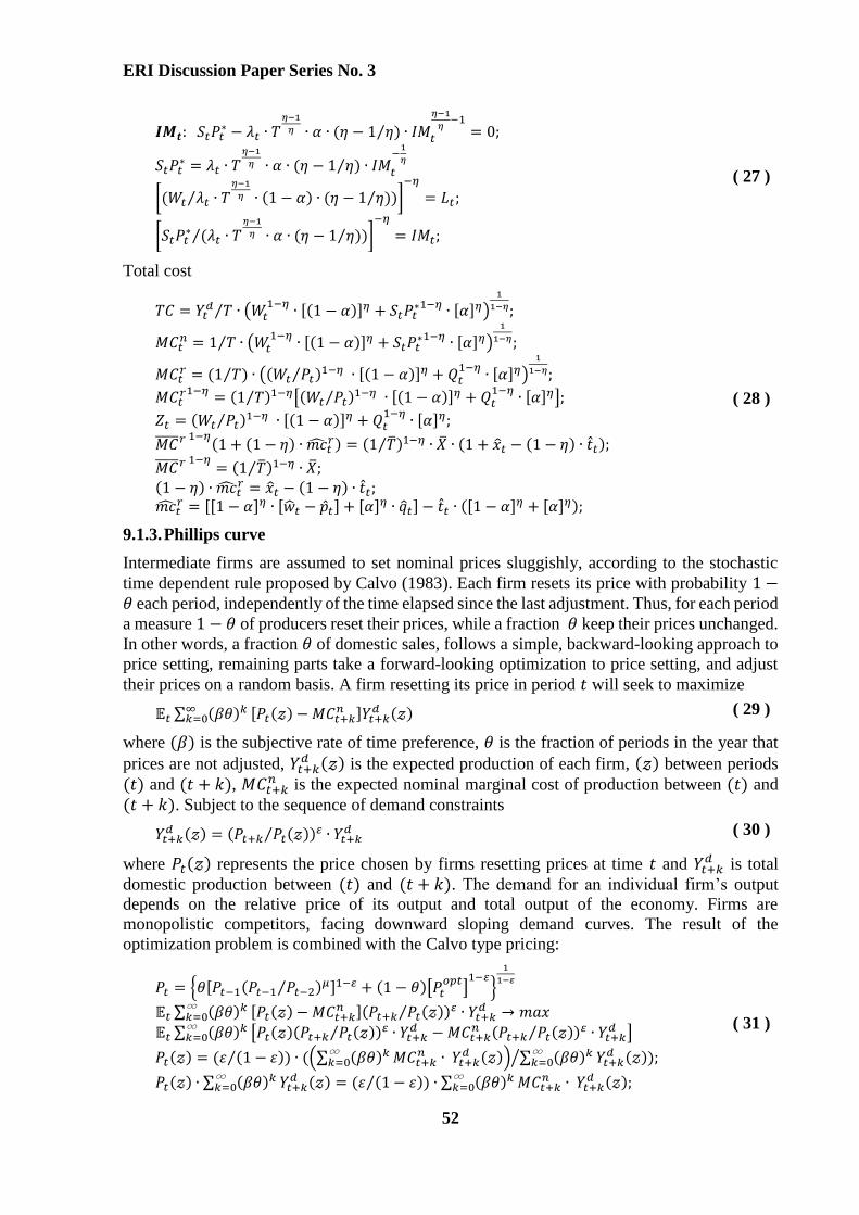
The first order conditions with respect to 𝐿𝑡 and 𝐼𝑀𝑡 are:

𝑳𝒕: 𝑊𝑡 = 𝜆𝑡 ∙ 𝑇𝜂−1

𝜂 ∙ (1 − 𝛼) ∙ (𝜂 − 1 𝜂⁄ ) ∙ 𝐿𝑡

−1

𝜂 ( 26 )


52

𝑰𝑴𝒕: 𝑆𝑡𝑃𝑡∗ − 𝜆𝑡 ∙ 𝑇

𝜂−1

𝜂 ∙ 𝛼 ∙ (𝜂 − 1 𝜂⁄ ) ∙ 𝐼𝑀𝑡

𝜂−1

𝜂−1

= 0;

𝑆𝑡𝑃𝑡∗ = 𝜆𝑡 ∙ 𝑇

𝜂−1

𝜂 ∙ 𝛼 ∙ (𝜂 − 1 𝜂⁄ ) ∙ 𝐼𝑀𝑡

−1

𝜂

[(𝑊𝑡 𝜆𝑡 ∙ 𝑇𝜂−1

𝜂 ∙ (1 − 𝛼) ∙ (𝜂 − 1 𝜂⁄ )⁄ )]−𝜂

= 𝐿𝑡;

[𝑆𝑡𝑃𝑡∗ (𝜆𝑡 ∙ 𝑇

𝜂−1

𝜂 ∙ 𝛼 ∙ (𝜂 − 1 𝜂⁄ ))⁄ ]−𝜂

= 𝐼𝑀𝑡;

( 27 )

Total cost

𝑇𝐶 = 𝑌𝑡𝑑 𝑇⁄ ∙ (𝑊𝑡

1−𝜂∙ [(1 − 𝛼)]𝜂 + 𝑆𝑡𝑃𝑡

∗1−𝜂 ∙ [𝛼]𝜂)1

1−𝜂;

𝑀𝐶𝑡𝑛 = 1 𝑇⁄ ∙ (𝑊𝑡

1−𝜂∙ [(1 − 𝛼)]𝜂 + 𝑆𝑡𝑃𝑡

∗1−𝜂 ∙ [𝛼]𝜂)1

1−𝜂;

𝑀𝐶𝑡𝑟 = (1 𝑇⁄ ) ∙ ((𝑊𝑡 𝑃𝑡⁄ )1−𝜂 ∙ [(1 − 𝛼)]𝜂 + 𝑄𝑡

1−𝜂∙ [𝛼]𝜂)

1

1−𝜂;

𝑀𝐶𝑡𝑟1−𝜂

= (1 𝑇⁄ )1−𝜂[(𝑊𝑡 𝑃𝑡⁄ )1−𝜂 ∙ [(1 − 𝛼)]𝜂 + 𝑄𝑡1−𝜂

∙ [𝛼]𝜂];

𝑍𝑡 = (𝑊𝑡 𝑃𝑡⁄ )1−𝜂 ∙ [(1 − 𝛼)]𝜂 + 𝑄𝑡1−𝜂

∙ [𝛼]𝜂;

𝑀𝐶̅̅̅̅̅𝑟 1−𝜂(1 + (1 − 𝜂) ∙ 𝑚�̂�𝑡

𝑟) = (1 �̅�⁄ )1−𝜂 ∙ �̅� ∙ (1 + 𝑥𝑡 − (1 − 𝜂) ∙ �̂�𝑡);

𝑀𝐶̅̅̅̅̅𝑟 1−𝜂= (1 �̅�⁄ )1−𝜂 ∙ �̅�;

(1 − 𝜂) ∙ 𝑚�̂�𝑡𝑟 = 𝑥𝑡 − (1 − 𝜂) ∙ �̂�𝑡;

𝑚�̂�𝑡𝑟 = [[1 − 𝛼]𝜂 ∙ [�̂�𝑡 − �̂�𝑡] + [𝛼]𝜂 ∙ �̂�𝑡] − �̂�𝑡 ∙ ([1 − 𝛼]𝜂 + [𝛼]𝜂);

( 28 )

9.1.3. Phillips curve

Intermediate firms are assumed to set nominal prices sluggishly, according to the stochastic

time dependent rule proposed by Calvo (1983). Each firm resets its price with probability 1 −𝜃 each period, independently of the time elapsed since the last adjustment. Thus, for each period

a measure 1 − 𝜃 of producers reset their prices, while a fraction 𝜃 keep their prices unchanged.

In other words, a fraction 𝜃 of domestic sales, follows a simple, backward-looking approach to

price setting, remaining parts take a forward-looking optimization to price setting, and adjust

their prices on a random basis. A firm resetting its price in period 𝑡 will seek to maximize

𝔼𝑡 ∑ (𝛽𝜃)𝑘∞𝑘=0 [𝑃𝑡(𝓏) − 𝑀𝐶𝑡+𝑘

𝑛 ]𝑌𝑡+𝑘𝑑 (𝓏) ( 29 )

where (𝛽) is the subjective rate of time preference, 𝜃 is the fraction of periods in the year that

prices are not adjusted, 𝑌𝑡+𝑘𝑑 (𝓏) is the expected production of each firm, (𝓏) between periods

(𝑡) and (𝑡 + 𝑘), 𝑀𝐶𝑡+𝑘𝑛 is the expected nominal marginal cost of production between (𝑡) and

(𝑡 + 𝑘). Subject to the sequence of demand constraints

𝑌𝑡+𝑘𝑑 (𝓏) = (𝑃𝑡+𝑘 𝑃𝑡(𝓏)⁄ )𝜀 ∙ 𝑌𝑡+𝑘

𝑑 ( 30 )

where 𝑃𝑡(𝓏) represents the price chosen by firms resetting prices at time 𝑡 and 𝑌𝑡+𝑘𝑑 is total

domestic production between (𝑡) and (𝑡 + 𝑘). The demand for an individual firm’s output

depends on the relative price of its output and total output of the economy. Firms are

monopolistic competitors, facing downward sloping demand curves. The result of the

optimization problem is combined with the Calvo type pricing:

𝑃𝑡 = {𝜃[𝑃𝑡−1(𝑃𝑡−1 𝑃𝑡−2⁄ )𝜇]1−𝜀 + (1 − 𝜃)[𝑃𝑡𝑜𝑝𝑡

]1−𝜀

}

1

1−𝜀

𝔼𝑡 ∑ (𝛽𝜃)𝑘∞𝑘=0 [𝑃𝑡(𝓏) − 𝑀𝐶𝑡+𝑘

𝑛 ](𝑃𝑡+𝑘 𝑃𝑡(𝓏)⁄ )𝜀 ∙ 𝑌𝑡+𝑘𝑑 → 𝑚𝑎𝑥

𝔼𝑡 ∑ (𝛽𝜃)𝑘∞𝑘=0 [𝑃𝑡(𝓏)(𝑃𝑡+𝑘 𝑃𝑡(𝓏)⁄ )𝜀 ∙ 𝑌𝑡+𝑘

𝑑 − 𝑀𝐶𝑡+𝑘𝑛 (𝑃𝑡+𝑘 𝑃𝑡(𝓏)⁄ )𝜀 ∙ 𝑌𝑡+𝑘

𝑑 ]

𝑃𝑡(𝓏) = (휀 (1 − 휀)⁄ ) ∙ ((∑ (𝛽𝜃)𝑘∞𝑘=0 𝑀𝐶𝑡+𝑘

𝑛 ∙ 𝑌𝑡+𝑘𝑑 (𝓏)) ∑ (𝛽𝜃)𝑘∞

𝑘=0 𝑌𝑡+𝑘𝑑 (𝓏)⁄ );

𝑃𝑡(𝓏) ∙ ∑ (𝛽𝜃)𝑘∞𝑘=0 𝑌𝑡+𝑘

𝑑 (𝓏) = (휀 (1 − 휀)⁄ ) ∙ ∑ (𝛽𝜃)𝑘∞𝑘=0 𝑀𝐶𝑡+𝑘

𝑛 ∙ 𝑌𝑡+𝑘𝑑 (𝓏);

( 31 )


53

∑ (𝛽𝜃)𝑘∞𝑘=0 𝑃𝑡(𝓏)𝑌𝑡+𝑘

𝑑 (𝓏) = �̅� ∙ �̅� ∙ ∑ (𝛽𝜃)𝑘∞𝑘=0 (1 + �̂�𝑡(𝓏) + �̂�𝑡+𝑘

𝑑 (𝓏));

휀 (1 − 휀)⁄ ∙ ∑ (𝛽𝜃)𝑘∞𝑘=0 𝑀𝐶𝑡+𝑘

𝑛 ∙ 𝑌𝑡+𝑘𝑑 (𝓏) = 휀 (1 − 휀)⁄ ∙ 𝑀𝐶̅̅̅̅̅ ∙ �̅� ∑ (𝛽𝜃)𝑘∞

𝑘=0 (1 +

𝑚�̂�𝑡+𝑘𝑛 + �̂�𝑡+𝑘

𝑑 (𝓏));

∑ (𝛽𝜃)𝑘∞𝑘=0 (1 + �̂�𝑡(𝓏) + �̂�𝑡+𝑘

𝑑 (𝓏)) = ∑ (𝛽𝜃)𝑘∞𝑘=0 (1 + 𝑚�̂�𝑡+𝑘

𝑛 + �̂�𝑡+𝑘𝑑 (𝓏));

((1 + �̂�𝑡(𝓏)) 1 − 𝛽𝜃⁄ )∑ (𝛽𝜃)𝑘∞𝑘=0 (�̂�𝑡+𝑘

𝑑 (𝓏)) = ∑ (𝛽𝜃)𝑘∞𝑘=0 (1 + 𝑚�̂�𝑡+𝑘

𝑛 +

�̂�𝑡+𝑘𝑑 (𝓏));

((1 + �̂�𝑡(𝓏)) (1 − 𝛽𝜃⁄ )) = ∑ (𝛽𝜃)𝑘∞𝑘=0 + ∑ (𝛽𝜃)𝑘∞

𝑘=0 (𝑚�̂�𝑡+𝑘𝑛 );

((1 + �̂�𝑡(𝓏)) (1 − 𝛽𝜃⁄ ) = (1 1 − 𝛽𝜃⁄ ) + ∑ (𝛽𝜃)𝑘∞𝑘=0 (𝑚�̂�𝑡+𝑘

𝑛 ); �̂�𝑡(𝓏) = (1 − 𝛽𝜃)∑ (𝛽𝜃)𝑘∞

𝑘=0 (𝑚�̂�𝑡+𝑘𝑛 );

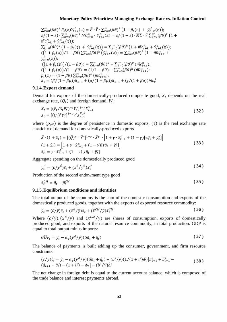
�̂�𝑡 = (𝛽 (1 + 𝛽𝜇)⁄ )�̂�𝑡+1 + (𝜇 (1 + 𝛽𝜇)⁄ )�̂�𝑡−1 + (𝜍 (1 + 𝛽𝜇)⁄ )�̂�𝑐𝑟𝑅

9.1.4. Export demand

Demand for exports of the domestically-produced composite good, 𝑋𝑡 depends on the real

exchange rate, (𝑄𝑡) and foreign demand, 𝑌𝑡∗:

𝑋𝑡 = [(𝑃𝑡 𝑆𝑡𝑃𝑡∗⁄ )−𝜏𝑌𝑡

∗]1−𝛾𝑋𝑡−1𝛾

𝑋𝑡 = [(𝑄𝑡)𝜏𝑌𝑡

∗]1−𝜌𝑥𝑑𝑋𝑡−1

𝜌𝑥𝑑

( 32 )

where (𝜌𝑥𝑑) is the degree of persistence in domestic exports, (𝜏) is the real exchange rate

elasticity of demand for domestically-produced exports.

�̅� ∙ (1 + 𝑥𝑡) = [(�̅�)𝜏 ∙ �̅�∗]1−𝛾 ∙ �̅�𝛾 ∙ [1 + 𝛾 ∙ 𝑥𝑡−1𝑑 + (1 − 𝛾)[𝜏�̂�𝑡 + �̂�𝑡

∗]]

(1 + 𝑥𝑡) = [1 + 𝛾 ∙ 𝑥𝑡−1𝑑 + (1 − 𝛾)[𝜏�̂�𝑡 + �̂�𝑡

∗]]

𝑥𝑡𝑑 = 𝛾 ∙ 𝑥𝑡−1

𝑑 + (1 − 𝛾)[𝜏�̂�𝑡 + �̂�𝑡∗]

( 33 )

Aggregate spending on the domestically produced good

�̂�𝑡𝑑 = (𝑐 𝑦

𝑑⁄ )�̂�𝑡 + (𝑥

𝑑𝑦

𝑑⁄ )�̂�𝑡

𝑑 ( 34 )

Production of the second endowment type good

𝑥𝑡𝐶𝑀 = �̂�𝑡 + �̅�𝑡

𝐶𝑀 ( 35 )

9.1.5. Equilibrium conditions and identities

The total output of the economy is the sum of the domestic consumption and exports of the

domestically produced goods, together with the exports of exported resource commodity:

�̂�𝑡 = (𝑐̅ �̅�⁄ )�̂�𝑡 + (�̅�𝑑 �̅�⁄ )𝑥𝑡 + (�̅�𝐶𝑀 �̅�⁄ )𝑥𝑡𝐶𝑀 ( 36 )

Where (𝑐̅ �̅�⁄ ), (�̅�𝑑 �̅�⁄ ) and (�̅�𝐶𝑀 �̅�⁄ ) are shares of consumption, exports of domestically

produced good, and exports of the natural resource commodity, in total production. GDP is

equal to total output minus imports:

𝐺�̂�𝑃𝑡 = �̂�𝑡 − 𝛼𝑦(�̅�𝑑 �̅�⁄ )(𝑖�̂�𝑡 + �̂�𝑡) ( 37 )

The balance of payments is built adding up the consumer, government, and firm resource

constraints:

(𝑐̅ �̅�⁄ )�̂�𝑡 = �̂�𝑡 − 𝛼𝑦(�̅�𝑑 �̅�⁄ )(𝑖�̂�𝑡 + �̂�𝑡) + (�̅�∗ �̅�⁄ )(1 (1 + 𝑖̅∗)�̅�⁄ )[𝜋𝑡+1∗ + �̂�𝑡+1

∗ −

(�̂�𝑡+1 − �̂�𝑡) − (1 + 𝑖̂𝑡∗) − �̂�𝑡] − (�̅�∗ �̅�⁄ )�̂�𝑡

∗ ( 38 )

The net change in foreign debt is equal to the current account balance, which is composed of

the trade balance and interest payments abroad.


54

9.2. Monetary policy operation and instruments

In 2007, monetary policy shifted into a different framework and made changes in monetary

policy operation. In along with these changes in operation, a policy rate was introduced and it

has become the principal instrument of monetary policy as well as the indicator of policy stance.

Policy rate is used as the discount rate at auction for 1 week CBB that has the lowest risk in

the interbank market. It is regulated consistent with the current economic situation and its

anticipated future tendency. In order to improve the transmission mechanism of monetary

policy, the interest rate corridor was introduced in March 2013. For the monetary policy

implementation, following instruments are used:

Central Bank’s Bill: 1 and 4 weeks of CBBs are used in open market operation. 1 week CBB

has two types of tender, which are policy rate tender with pre-announced allotment volume,

policy rate tender with free allotment volume. 4 weeks CBBs are tendered with variable interest

rate tender with ceiling rate and pre-announced allotment volume. The volume of CBB is

approved by the governor of the BoM.

Reserve requirements: It is one of the policy instruments used to monitor money supply and

manage liquidity within the interbank market. The banks are required to maintain reserves

holdings under the arrangement facilitates, as they always have the necessary funds at their

disposal. The reserve requirement system is averaged on maintenance period of 2 weeks which

allows banks to determine the amount of funds held on the current account of the central bank.

According to the Central Bank Law, this ratio must not be higher than 30 percent of bank’s total

assets.

Overnight repo: The central bank offers the standing facility of overnight repo to fulfill the

reserve requirements of banks, with certain collateral. The overnight repo rate is ceiling of the

corridor or 2 points higher than the policy rate and volume of the loan shall not exceed the

required reserve. The maturity is from closing of the clearing settlement of current day to

opening of clearing settlement of the following working day.

Repo: Repo financing is a deal whereby central bank purchases securities under the condition

to resell at a predetermined price on the specified date. The repo financing rate is set to 0.5

percentage points above the policy rate. The accepted securities are CBBs, government bonds,

and Mongolian Mortgage Corporation bonds.

Intra-day repo: The purpose of the intra-day facility is to maintain bank’s liquidity and to keep

the ordinary function of the banking payment system as the source of funds to be obtained

during the trading day. The BoM do not issue interest earnings from this type of facility and

repo is collateralized with securities accepted by the central bank.

10. References

Adolfson, M., Laseen, S., Linde, J., & Villani, M. (2008). Evaluating an estimated new

Keynesian small open economy model. Journal of Economic Dynamics and Control,

2690–721.

Aizenman, Joshua, & Michael, H. (2008). Inflation Targeting and Real Exchange Rates in

Emerging Markets. NBER Working Paper.

Allen, M., Rosenberg, C., Keller, C., Setser, B., & Roubini, N. (2002). A Balance Sheet

Approach to Financial Crisis. IMF Working paper, WP/02/210.


55

Avralt-Od, P., & Davaadalai, B. (2010). An assessing asymmetric impact of exchange rate on

inflation. Research yearbook of Mongolbank, 5.

Avralt-Od, P., Davaadalai, B., & Bumchimeg, G. (2011). Coordination Monetary and Fiscal

policy: DSGE model. Research yearbook of Mongolbank, 6, pp. 419-452.

Bahmani-Oskooee, M., & Kutan, A. M. (2008). Are Devaluations Contractionary in Emerging

Economies of Eastern Europe? Economic Change and Resctructuring, 41(1), 61-74.

Ball, L. (2008). Policy Rules and External Shocks. Central Bank of Chile Working Papers.

Ball, L. M. (1999). Monetary Policy Rules. In J. B. Taylor (Ed.). University of Chicago Press.

Bank of Mongolia. (2011). Annual report. Ulaanbaatar.

Bank of Mongolia. (2012, December). Monthly statistical bulletin.

Batini, N., Kuttner, K., & Laxton, D. (2005). Does Inflation Targeting work in Emerging

Markets? In I. F. Fund, World Economic Outlook. Washington.

Batsukh, T. (2008). Anti-inflation macro economic policy. Ulaanbaatar: Open Society Forum.

Berg, Andrew, Karam, P., & Laxton, D. (2006). A practical model-based approach to monetary

policy analysis-overview. IMF Working Paper.

Calvo, G. A., & Reinhart, C. M. (2000). Fear of Floating. NBER working papers.

Campbell, J., & Mankiw, N. (1989). Consumption, Income, and Interest Rates: Reinterpreting

the Time Series Evidence. NBER Macroeconomics Annual, 185-216.

Davaajargal, B. (2005). A defining time lagged effect of monetary policy on inflation. Research

yearbook of Mongolbank, 3.

Dong, W. (2008). Do central banks respond to exchange rate movements? Some new evidence

from structural estimation. Bank of Canada Working Paper, 2008–24.

Engel, C. (2011). Currency Misalignments and Optimal Monetary Policy: A Reexamination.

American Economic Review.

Filardo, A., Ma, G., & Mihaljek, D. (2011). Exchange rates and monetary policy frameworks

in EMEs. BIS papers.

Galí, J., & Monacelli, T. (2005). Monetary Policy and Exchange Rate Volatility in a Small

Open Economy. Review of Economic Studies, 707–734.

Gan-Ochir, D. (2009). Exchange rate pass through to inflation in Mongolia. Research yearbook

of Mongolbank, 7, pp. 286-308.

Gan-Ochir, D. (2011). The relationship between nominal exchange rate of togrog and inflation.

Research yearbook of Mongolbank, 6, pp. 389-404.

Ho, C., & McCanley, R. N. (2003). Living with flexible exchange rates: issues and recent

experience in inflation-targeting emerging market economies. BIS Working Papers,

130.

IMF. (2011). Mongolia: Financial System Stability Assessment. Washington, D.C.

Khulan, A. (2005). An assessing factors on inflation. Research yearbook of Mongolbank, 3.

Kirsanova, T., Campbell, L., & Wren-Lewis, S. (2003). Should Central Bank Target Consumer

Price or the Exchange Rate. The Economic Journal, 208-231.


56

Mishkin, F. (2000). Inflation Targeting for Emerging Market Countries. American Economic

Review, 105–9.

Morón, E., & Winkelried, D. (2005). Monetary Policy Rules for Financially Vulnerable

Economies. Journal of Development Economics, 25–51.

Mussa, M., Masson, P., Swoboda, A., Jadresic, E., Mauro, P., & Berg, A. (2000). Exchange

Rate Regimes in an Increasingly Integrated World Economy. Occasional Paper, 193.

Narantuya, C., Davaasuren, S., Otgontugs, B., & Tuvshintugs, B. (2009). Financial and

economic crisis: Mongolia. Ulaanbaatar: Open Society Forum.

Otker-Robe, I., & Vavra, D. (2007). Moving to Greater Exchange Rate Flexibility Operational

Aspects based on Lessons from Detailed Country Experiences. Occasional Paper, 256.

Parrado, E. (2004). Inflation Targeting and Exchange Rate Rules in an Open Economy. IMF

Working Paper.

Reinhart, C. M., & Rogoff, K. S. (2004). The Modern History of Exchange rate Arrangements:

A Reinterpretation. Quarterly Journal of Economics, CXIX(1).

Roger, S., Restrepo, J., & Garcia, C. (2009). Hybrid Inflation Targeting Regimes. IMF Working

Paper.

Rogoff, S. K., Husain, M. A., Mody, A., Brooks, R., & Oames, N. (2003). Evolution and

Performance of Exchange Rate Regimes . IMF Working Paper, WP/03/243.

Smets, F., & Wouters, R. (2002). Openness, Imperfect Exchange Rate Pass-through and

Monetary Policy. Journal of Monetary Economics, 947–81.

Stone, M., Roger, S., Shimizu, S., Nordstrom, A., Kisinbay, T., & Restrepo, J. (2009). The Role

of the Exchange Rate in Inflation-Targeting Emerging Economies. Occasional Paper,

267.

Svensson, L. (2000). Open economy inflation targeting. Journal of International Economics,

50, 155-183.

Taylor, J. (1993). Discretion versus policy rule in pracrice. Carnegiei-Rochester Conference on

Public Policy . 195-214.

Tuvshinjargal, D. (2010). Time inconsistency and Central bank independence in Mongolia.

Annual conference of IFE. Ulaanbaatar.

Tuvshintugs, B. (2009). Global financial and economic crisis and Mongolian financial market.

Ulaanbaatar: Open Society Forum.

MONETARY POLICY PRIORITIES: MANAGING EXCHANGE RATE …

Documents

Transcript of MONETARY POLICY PRIORITIES: MANAGING EXCHANGE RATE …