Monetary Policy, Indeterminacy and Learning∗

George W. Evans

University of Oregon

Bruce McGough

Oregon State University

October 11, 2003

Abstract

The development of tractable forward looking models of mone-

tary policy has lead to an explosion of research on the implications of

adopting Taylor-type interest rate rules. Indeterminacies have been

found to arise for some specifications of the interest rate rule, raising

the possibility of increased economic fluctuations due to a dependence

of expectations on extraneous “sunspots.” Separately, recent work by

a number of authors has shown that sunspot equilibria previously

thought to be unstable under private agent learning can in some cases

be stable when the observed sunspot has a suitable time series struc-

ture. In this paper we generalize the “common factor” technique, used

in this analysis, to examine standard monetary models that combine

forward looking expectations and predetermined variables. We con-

sider a variety of specifications that incorporate both lagged and ex-

pected inflation in the Phillips Curve, and both expected and inertial

elements in the policy rule. We find that some policy rules can indeed

lead to learnable sunspot solutions and we investigate the conditions

under which this phenomenon arises.

JEL classification: E52, E32, D83, D84.

Keywords: Monetary Policy, sunspots, expectations, learning, stabil-

ity.

∗We are indebted to Stephen G.F. Hall, Seppo Honkapohja and Julien Matheron forvaluable comments. This material is based upon work supported by the National ScienceFoundation under Grant No. 0136848.

1

1 Introduction

The development of tractable forward looking models of monetary policy,together with the influential work of (Taylor 1993), has lead to an explosionof research on the implications of adopting Taylor-type interest rate rules.These rules take the nominal interest rate as the policy instrument and directthe central bank to set this rate according to some simple (typically linear)dependence on current, lagged, and/or expected inflation and output gap,and possibly on an inertial term to encourage interest rate smoothing.

While these simple policy rules for many reasons are advantageous toboth researchers and policy makers, it has been noted by some authors,e.g. (Bernanke and Woodford 1997), (Woodford 1999) and (Svensson andWoodford 1999), that the corresponding models exhibit indeterminate steady-states for large regions of the reasonable parameter space. This presence ofindeterminacy is thought undesirable because associated with each indeter-minate steady-state is a continuum of sunspot equilibria, and the particularequilibrium on which agents ultimately coordinate may not exhibit wantedproperties.

Though having their informal origins in Keynes’ notion of animal spirits,analysis of sunspots has, in the past, been couched principally in the theoreti-cal literature. However, applied macroeconomists began to take notice when,in the mid nineties, (Farmer and Guo 1994) showed that calibrated real busi-ness cycle models, modified to include externalities or other non-convexities,exhibited sunspots; and furthermore, these sunspots could be used to ex-plain fluctuations at business cycle frequencies. This applied interest hasspread to the literature on monetary policy, and, in an empirical sense, hasculminated with the argument of (Clarida, Gali, and Gertler 2000) that thevolatile inflation and output of the seventies may have been due to sunspotphenomena. In particular, they combine a standard forward-looking “NewKeynesian” IS-AS model1 with a simple estimated forward-looking Taylorrule, using data from the 1960’s and 1970’s, and find that the correspondingsteady-state is indeterminate; they conclude that the fluctuations in outputgap and inflation may be well explained by agents coordinating on a volatilesunspot equilibrium.

1This model has also been called the “New Phillips Curve” or “optimizing IS-AS”model, and is obtained as a linearization of an optimimizing equilibrium model with“Calvo” pricing. For discussion, derivation and citations to the earlier literature, see(Clarida, Gali, and Gertler 1999), (Woodford 1999) and (Woodford 2003).

2

The existence of sunspot equilibria raises the question of whether it isplausible that agents will actually coordinate on them. One natural criterionfor this is that the sunspot equilibria should be stable under adaptive learn-ing.2 Although it has been shown by (Woodford 1990) that stable sunspotscan exist in simple overlapping generations models,3 the sunspots in manycalibrated applied models are lacking this necessary stability. For example(Evans and Honkapohja 2001) show that sunspots in the Farmer-Guo modelare unstable, and (Evans and McGough 2002a) describe a stability puzzlesurrounding the lack of stable indeterminacies in a host of non-convex RBC-type models.4

The existence of indeterminacies in monetary models, together with theinstability of indeterminacies in RBC-type models, raises a natural question:Are sunspot equilibria in the New Keynesian models stable under learning?This specific question has been addressed by (Honkapohja and Mitra 2001),who consider a purely forward looking AS equation (“ Phillips” curve) andanalyze a variety of interest rules including those dependent on current,lagged, and expected inflation and output gap, and those also dependenton an interest rate smoothing term. They find that if the interest rate de-pends only on expected inflation and expected output gap then there canexist stable equilibria that depend on finite state sunspots; otherwise, thesunspot equilibria they consider are not learnable.5

Independent of the monetary policy literature, work on multiple equilib-ria and stability in macroeconomic models has continued, and recent researchhas emphasized that stability under learning of sunspots can depend uponthe way in which a particular equilibrium is viewed, or represented. (Evansand Honkapohja 2003c) found that finite state sunspots in a simple forwardlooking model can be stable even though previous research had suggested

2Eductive approaches could also be considered. See, for example, (Guesnerie 1992),(Evans and Guesnerie 2003) and (Desgranges and Negroni 2001). Stability under eductivelearning appears to be somewhat more stringent than stability under adaptive learning.

3For the local stability conditions see (Evans and Honkapohja 1994) and (Evans andHonkapohja 2003b).

4Other examples of stable sunspot equilibria include (Howitt andMcAfee 1992), (Evans,Honkapohja, and Romer 1998), (Evans, Honkapohja, and Marimon 2001) and (Evans andMcGough 2003).

5For these models stability under learning of “fundamental” (minimal state variable)solutions has been studied by (Bullard and Mitra 2003), (Evans and Honkapohja 2003d)and others. For a survey with references see (Evans and Honkapohja 2003a). An importantearly instability result was obtained by (Howitt 1992).

3

that no stable sunspots exist in these models. The apparent paradox is re-solved as follows: all sunspot equilibria in these models can be represented asa linear dependence on lagged endogenous variables and a sunspot variabletaking the form of a martingale difference sequence. These representationsare always unstable under learning. However, when the sunspot is a finitestate Markov process, the associated equilibrium is also finite state and thushas an alternate representation depending solely on the sunspot. When rep-resented in this manner, the associated learning dynamics indicate stabilityfor some (but not all) regions of the parameter space.

In (Evans and McGough 2003), we studied sunspot equilibria in a uni-variate stochastic linear forward looking model that incorporates a lag. Wefound that any given equilibrium may be viewed, or represented, in two fun-damentally different ways: in the usual way, as a linear dependence on onceand twice lagged endogenous variables and on a sunspot having zero condi-tional mean; and in a new way, on once lagged endogenous variables and ona sunspot exhibiting serial correlation. We referred to the usual way of view-ing sunspots as the “general form” representation of the equilibrium, and tothe new way of viewing sunspots as the “common factor” representation ofthe equilibrium.6 We found that the stability of the equilibrium in questiondepended on the chosen representation. In particular, for the model we con-sidered, stable common factor sunspots were found to exist in abundance,even though, as was already well known, there exist no stable general formsunspots.

This new line of research indicates the need for careful analysis of sunspotstability in applied models. Every sunspot equilibrium has a common factor

representation, and the stability properties of common factor representations

are different from their general form counterparts. Thus, stability analysismust incorporate both general form and common factor representations. Inthis paper, we generalize common factor analysis to apply to standard mod-els of monetary policy, and carefully investigate the stability of the resultingrepresentations. We follow (Bullard and Mitra 2002) and (Honkapohja andMitra 2001) by specifying a simple New Keynesian IS-AS model, except that,for added generality, as in (Galí and Gertler 1999) and much applied work, we

6In (Evans and McGough 2002b) we show that common factor sunspot representationsexist in some cases where finite state Markov sunspot solutions do not exist.We remark that (Evans and McGough 2002b) and (Evans and McGough 2003) focus on

models with real roots, but we show elsewhere that coomon factor sunspots representationsexist more generally when there are complex roots.

4

allow for some dependence on lagged inflation in the Phillips curve. We closethe model with a variety of interest rate rules: like Bullard and Mitra, weconsider rules depending on current, lagged, and expected inflation; and likeHonkapohja and Mitra, we also consider rules depending on lagged nominalinterest rates. For each model we consider three calibrations of the IS-ASstructure, as well as some alternative parameter values. Analytic resultsare, in general, unavailable, and so we test stability numerically by consid-ering, for each calibration, a lattice over the space of policy parameters. Ateach point in the lattice, indeterminacy and stability of the correspondingequilibria are examined. Our main result supports the findings and adviceof Honkapohja and Mitra, and indeed it makes their cautionary note moreurgent: All models in which the policy rule depends on some form of expec-tations of future variables exhibit stable common factor sunspots for someparameter values. To be sure, these parameter values are not always rea-sonable, but, in some cases, they closely match calibrations. Furthermore,these stable sunspots exist even when the policy rule also depends on otheraggregates, such as current inflation or output, and lagged interest rate. Wealso find that no general form sunspots are stable, thus emphasizing theimportance of analyzing common factor representations.

This paper is organized as follows. Section two presents the various mon-etary models under consideration, as well as the associated learning theoryand the extension of common factor analysis to monetary models. To con-serve space and facilitate comprehension, we include explicit computationsof equilibrium representations in the Appendix and for only one policy rule,and simply note that the remaining policy rules can be analyzed in a similarfashion. Section three contains the results of our investigations. The policyrules are classified into four types and discussed in separate subsections. Ineach case we consider numerous permutations of calibration, Phillips curvestructure, indeterminacy nature, and representation type, and thus a carefulcatalog of all possible results would be tedious if not infeasible. Therefore, weprovide a summary of the main features followed by a more careful discussionof the particularly interesting results. Section four concludes.

2 Theory

In this section we develop the theory necessary to analyze the stability ofsunspot equilibria. We begin by specifying the models of interest. Then, for

5

expedience, we choose a particular specification and develop the associatedequilibrium representations and learning analysis. It is straightforward tomodify this developed theory for application to other model specifications,and thus we omit the details concerning these other models. We initiallydevelop the theory under the rational expectations assumption. Then, be-ginning in Section 2.4, we relax this assumption and study the stability ofthe solutions under adaptive learning.

2.1 Monetary Models and Policy Rules

We explore the possibility of existence of stable sunspots using several vari-ants of the New Keynesian Monetary model. All specifications have in com-mon the following forward looking IS-AS curves:

IS : xt = −φ(it − Etπt+1) + Etxt+1 + gt (1)

AS : πt = β(γEtπt+1 + (1− γ)πt−1) + λxt + ut (2)

Here xt is the proportional output gap, πt is the inflation rate, and gt andut are independent, exogenous, stationary, zero mean AR(1) shocks withdamping parameters 0 ≤ ρg < 1 and 0 ≤ ρu < 1 respectively.

Equation (1) is the “IS” relationship obtained by log-linearizing the Eulerequation for consumer optimization and using the GDP identity. This yieldsa unit coefficient on Etxt+1.

7 When γ = 1, equation (2) is the pure forward-looking New Keynesian “AS” relationship based on “Calvo pricing,” andemployed in (Clarida, Gali, and Gertler 1999) and Ch. 3 of (Woodford 2003).8

Here 0 < β < 1 is the discount factor. Again, this equation is obtained asthe linearization around a steady state. The specification of the AS curve inthe case 0 < γ < 1 incorporates an inertial term and is similar in spirit to(Fuhrer and Moore 1995), the Section 4 model of (Galí and Gertler 1999),and the Ch. 3, Section 3.2 model of (Woodford 2003), each of which allowsfor some backward looking elements. Models with 0 < γ < 1 are often called“hybrid” models, and we remark that in some versions, such as (Fuhrer andMoore 1995), β = 1, so that the sum of forward and backward lookingcomponents sum to one, while in other versions β < 1 is possible.

The region and nature of a model’s indeterminacy depends critically onthe specification of the policy rule. To better understand the role of this

7See, for example, Chapter 2 and Chapter 4, Section 1, of (Woodford 2003).8For the version with mark-up shocks see (Woodford 2003) Chapter 6, Section 4.6.

6

specification, we analyze a number of policy rules, which we parameterize asfollows:

PR1 : it = αππt + αxxt (3)

PR′

1 : it = απEtπt + αxEtxt (4)

PR2 : it = αππt−1 + αxxt−1 (5)

PR3 : it = απEtπt+1 + αxEtxt+1 (6)

PR4 : it = θit−1 + (1− θ)απEtπt+1 + (1− θ)αxxt (7)

PR1, PR′

1, PR2, and PR3 are the rules examined by (Bullard and Mitra2002). We have omitted the intercepts for convenience, and in each policyrule πt can be interpreted as the deviation of inflation from its target. Theseare all Taylor-type rules in the spirit of (Taylor 1993). We assume throughoutthat απ, αx ≥ 0 and thus the αππt term in PR1 indicates the degree to whichmonetary policy authorities raise nominal interest rates in response to anupward deviation of πt from its target. PR1 assumes that current data oninflation and the output gap are available to policymakers when interestrates are set. Given the criticism that this assumption is not realistic, apoint emphasized in (McCallum 1999), (Bullard and Mitra 2002) look atthree natural alternatives: a slight modification yields PR′

1 in which policymakers condition their instrument on expected values of current inflation andthe output gap; in PR2 policy makers respond to the most recent observedvalues of these variables; and in PR3 they respond instead to forecasts offuture inflation and the output gap.9 Finally, PR4 is the rule examined inthe theoretical part of (Clarida, Gali, and Gertler 2000), and is the simplestform of the empirical interest rate rules that they estimate. A parametervalue 0 < θ < 1 corresponds to inertia in interest rate setting, with policy-makers responding gradually to changes in information.

2.2 Determinacy

As usual, the model is said to be determinate if there is a unique nonexplosiveREE and indeterminate if there are multiple nonexplosive solutions (though

9Because at the moment we are assuming rational expectations and a common infor-mation set, we do not need to specify whose forecasts are represented in the interest raterules (4), (6) and (7). We will return to this matter when we discuss the economy underlearning.

7

we will see below that this definition can be refined in a helpful way).10

The determinacy of a model can be analyzed by writing the reduced formequation as a discrete difference equation with the associated extraneousnoise terms capturing the errors in the agents’ forecasts of the free variables.If the nonexplosive requirement of a rational expectations equilibrium pinsdown the forecast errors, that is, if the dimension of the unstable manifoldis equal to the number of free variables, then the model is determinate. Onthe other hand, if the errors are not pinned down, that is, if the dimension ofthe unstable manifold is less than the number of free variables, these forecasterrors can capture extrinsic fluctuations in agents’ expectations that are notinconsistent with rationality. In this case, multiple equilibria exist; thesetypes of equilibria are sometimes called sunspots.

To illustrate our methodology, consider PR1 or PR3. Combining thepolicy rule (3) or (6) with (1) and (2) leads to the first-order reduced form

H

xt

πt

πt−1

gtut

= F

Etxt+1Etπt+1

πt

gt+1ut+1

−

000wg

t

wut

.

The specific form of F,H are given in the Appendix for PR1. Let the freevariables be written yt = (xt, πt)

′, so that εt = yt−Et−1yt is the forecast error,thus capturing potential sunspots. Writing also yt = (xt, πt, πt−1, gt, ut)

′ andwt = (wg

t , wut )

′ the model can be rewritten as

yt = F−1Hyt−1 + F−1Mwt +Nεt (8)

for suitable M,N . Here we are using the fact that F is invertible. Note thatby virtue of the rational expectations assumption εt is a martingale differencesequence, i.e. a stochastic process such that Etεt+1 = 0.

Recall that a Rational Expectations Equilibrium (REE) is any process ytthat satisfies the reduced form equations and is nonexplosive. The aboveanalysis has shown that if yt is an REE then there is a martingale differencesequence (mds) εt such that the associated process yt solves (8). However,

10By “nonexplosive” we mean that the conditional expectation of the absolute value offuture variables is uniformly bounded over the horizon. For a detailed discussion of thisand related concepts see (Evans and McGough 2003).

8

there is no guarantee that a given mds εt yields a nonexplosive solution; it isprecisely this issue that is addressed by the nature of the indeterminacy.

To understand for which mds εt the model is nonexplosive, we assumethat F−1H is diagonalizable and factor it as F−1H = S(Λ⊕ ρ)S−1. Here weemploy the direct sum notation

A⊕B =

(A 00 B

)

for matrices A and B. ρ is a diagonal 2 × 2 matrix with diagonal elementsρg and ρu and Λ contains the remaining three eigenvalues of F−1H. We thenchange coordinates to zt = S−1yt, thus allowing us to rewrite (8) as

zt = (Λ⊕ ρ)zt−1 + wt + εt, (9)

where wt = S−1F−1Mwt and εt = S−1Nεt. If the eigenvalues of F−1H areall real then the columns of S are the corresponding linearly independenteigenvectors. If two eigenvalues are complex then we assume that the matrixof eigenvectors, S and the matrix of eigenvalues Λ are altered to allow for amatrix factorization with real entries. This can be achieved via the followingobservation: If A is a real 2× 2 matrix with complex eigenvalues µ± iν andcomplex eigenvectors u± iv then

A = S

[µ −νν µ

]S−1

where the columns of S are v and u. If A is n×n then it can be decomposedsimilarly as SDS−1 with D a block diagonal matrix with the real eigenvaluesand 2 × 2 blocks corresponding to the complex eigenvalues on its diagonal.Also, here and throughout the paper, the eigenvalues in Λ are assumed or-dered in decreasing magnitude.

Now the conditions for determinacy are clear. If λ1 and λ2 lie outsidethe unit circle, then nonexplosiveness requires zit = 0 for i = 1, 2. Thusthe forecast errors are pinned down by the requirement that wit + εit = 0for i = 1, 2; that is, the dimension of the unstable manifold, which in thissimple linear framework is the direct sum of the eigenspaces correspondingto the explosive eigenvalues, is two, and there is a unique mds εt such thatthe associated process yt is nonexplosive.

If |λ1| > 1 and |λ2| < 1 then the only implied restriction is that z1t = 0.The forecast errors must satisfy w1t+ ε1t = 0 but are otherwise unrestricted.

9

Thus there is a one dimensional continuum of equilibria, and, consequently,we say the model exhibits order one indeterminacy. Finally, if λi is in theunit circle for all i, the process yt is nonexplosive regardless of the mds εt.There is a two dimensional continuum of equilibria, and we say the modelexhibits order two indeterminacy.

We have focused on cases of determinacy and indeterminacy, but oneother possibility should be noted. If |λ3| > 1, so that there are three rootsoutside the unit circle, then the model is explosive: there exist no nonexplo-sive solutions and with probability one at least one of the components of yttends to infinity in absolute value as t → ∞.

2.3 Representations

A rational expectations equilibrium representation (REER) is a discrete dif-ference equation, any solution to which is an REE. As is now well known,see e.g. Chapters 8 and 9 of (Evans and Honkapohja 2001), (Evans andHonkapohja 2003c) and (Evans and McGough 2003), a given REE may havemany representations, and the stability of the REE under learning may berepresentation dependent. In this subsection we construct the representationsof interest, noting that the particular form of the representation depends onthe nature of the indeterminacy.

Assume first that for i = 1, 2 we have |λi| > 1 and also assume that|λ3| < 1. For the solution to be nonexplosive the mds sunspots ε1t andε2t must be chosen so that εit + wit = 0 for i = 1 and 2. The associatedrepresentation is given by

yt = −(S112 )−1

(0 S13

0 S23

)yt−1 − (S11

2 )−1S142 gt, (10)

where for convenience, we write gt = (gt, ut)′. Here and in the sequel, Sij =

(S−1)ij and

Sij

k =

(Sij Sij+1

Skj Skj+1

).

Thus, in the determinate case, the unique nonexplosive solution takes theform

yt = a+ byt−1 + cgt, (11)

where a = 0 because in the structural equations we have omitted intercepts.We include the intercept term a here and below because under learning agentswill be assumed to estimate its value.

10

2.3.1 Order One Indeterminacy.

Order one indeterminacy occurs when |λ1| > 1 and the remaining eigenvalueshave norm less than one. Notice this implies λ1 is real; however λi for i > 1may be complex. For reasons discussed below, in the indeterminate case, weonly consider real eigenvalues. To obtain a nonexplosive solution, we requirethat z1t = 0, and that the mds εt satisfy ε1t + w1t = 0. We now proceed todevelop the general form and common factor representations.

General Form Representations: As is shown in the Appendix, imposingthe restriction z1t = 0 for all t leads to General Form (GF) representations

yt = a + byt−1 + hyt−2 + cgt + f gt−1 + eξt. (12)

where ξt is an arbitrary one-dimensional mds and a = 0. There are actuallytwo representations of this form, i.e. two distinct nontrivial sets of parametercoefficients (b, h, c, d) which yield solutions of this form. These are obtainedby combining z1t = 0 with either the i = 2 or i = 3 equation from (9), i.e.with

zit = λizit−1 + wit + εit (13)

and then using the definition of zt to rewrite the equation in term of yt. TheAppendix gives details. Note that the General Form representations expressthe REE as a dependence of the endogenous variables on two lags, currentand lagged intrinsic noise, and a sunspot exhibiting no serial correlation.11

Common Factor Representations: As with the general form representa-tion we impose z1t = 0 and that the mds εt satisfy ε1t + w1t = 0. There willbe two Common Factor (CF) representations, again obtained by combiningz1t = 0 with (13) for either i = 2 or i = 3. However, we now rewrite (13) as

zit = (1− λiL)−1(wit + εit).

We interpret the noise term on the right to be a sunspot ζt and thus writezit = ζt with

ζ t = λiζt−1 + εt,

where εt = wit + εit. Note that since only one dimension of εt is restricted,we can take εt to be an arbitrary univariate mds. Combining this with the

11Our method for computing the GF representations (12) is closely related to the so-lution method for the “irregular case” described in Chapter 10, Appendix 2, of (Evansand Honkapohja 2001) and which was used to obtain the VARMA solutions given in(Honkapohja and Mitra 2001).

11

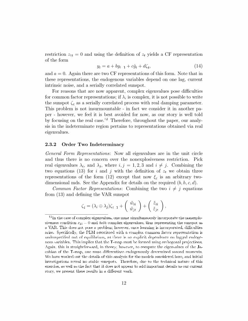
restriction z1t = 0 and using the definition of zt yields a CF representationof the form

yt = a+ byt−1 + cgt + dζt, (14)

and a = 0. Again there are two CF representations of this form. Note that inthese representations, the endogenous variables depend on one lag, currentintrinsic noise, and a serially correlated sunspot.

For reasons that are now apparent, complex eigenvalues pose difficultiesfor common factor representations; if λi is complex, it is not possible to writethe sunspot ζt as a serially correlated process with real damping parameter.This problem is not insurmountable - in fact we consider it in another pa-per - however, we feel it is best avoided for now, as our story is well toldby focusing on the real case.12 Therefore, throughout the paper, our analy-sis in the indeterminate region pertains to representations obtained via realeigenvalues.

2.3.2 Order Two Indeterminacy

General Form Representations: Now all eigenvalues are in the unit circleand thus there is no concern over the nonexplosiveness restriction. Pickreal eigenvalues λi, and λj, where i, j = 1, 2, 3 and i �= j. Combining thetwo equations (13) for i and j with the definition of zt we obtain threerepresentations of the form (12) except that now ξt is an arbitrary two-dimensional mds. See the Appendix for details on the required (b, h, c, d).

Common Factor Representations: Combining the two i �= j equationsfrom (13) and defining the VAR sunspot

ζt = (λi ⊕ λj)ζt−1 +

(wit

wjt

)+

(εitεjt

),

12In the case of complex eigenvalues, one must simultaneously incorporate the nonexplo-siveness condition z1t = 0 and both complex eigenvalues, thus representing the sunspot as

a VAR. This does not pose a problem; however, once learning is incorporated, difficulties

arise. Specifically, the PLM associated with a complex common factor representation is

underspecified out of equilibrium, as there is no explicit dependence on lagged endoge-

nous variables. This implies that the T-map must be formed using orthogonal projections.

Again, this is straightforward, in theory; however, to compute the eigenvalues of the Ja-

cobian of the T-map, one must differentiate endogenously determined second moments.

We have worked out the details of this analysis for the models considered here, and initial

investigations reveal no stable sunspots. Therefore, due to the technical nature of this

exercise, as well as the fact that it does not appear to add important details to our current

story, we present these results in a different work.

12

we obtain CF representations of the form (14) except that now of course ζtis

two-dimensional. Again, further details on (b, c) are given in the Appendix.

2.3.3 Discussion

For PR1 and PR3 with γ = 1 the procedure to provide solution representa-tions could be simplified since πt−1 no longer appears in the structural equa-tions. πt−1 could thus be dropped from the first-order form of the model.However, the above analysis does also cover this case. If γ = 1 then in thedeterminate case b = 0. Similarly, when γ = 1 and the model is indetermi-nate, the general form representations satisfy h = 0. In this case one of theCF representations satisfies b = 0, with a serially correlated sunspot ζ

t, and

the other CF representation has a serially uncorrelated sunspot with b �= 0.We also provide a brief discussion of REERs under policy rules PR2 and

PR4. In the case of PR2, given by (5), the state variable in the first-orderform must be enlarged to include xt−1. Then yt = (xt, πt, πt−1, xt−1, gt, ut)

′

and zt becomes 6 × 1. The methodology for obtaining solutions is analo-gous and in fact the form of the solution representations for yt = (xt, πt)is as above. For PR4, given by (7), the state vector is written as yt =(xt, πt, it, πt−1, it−1, gt, ut)

′, zt is 7 × 1 and yt = (xt, πt, it)′. However, the

procedure for determining REERs remains analogous.We close this section with a brief remark on an aspect of the time series

properties of sunspot equilibria. Consider the CF representations (14). Ifthe exogenous sunspot variable ζ

tis independent of the intrinsic shocks gt,

then it is easily verified that the endogenous variables yt have larger variancesthan are present in the corresponding minimal state variable solution yt =a + byt−1 + cgt. Policy makers that aim to minimize output and inflationvolatility would thus want to avoid interest rate rules consistent with theexistence of CF sunspot solutions, at least if these solutions are stable underlearning. We now turn to this issue, i.e. to the question of the stability ofthe various solutions under least squares learning.

2.4 Learning

We use expectational stability as our criterion for judging whether agents maybe able to coordinate on specific solutions, including in particular sunspotequilibria. This is because, for a wide range of models and solutions, E-stability has been shown to govern the local stability of rational expectations

13

equilibria under least squares learning. In many cases this correspondencecan be proved, and in cases where this cannot be formally demonstrated the“E-stability principle” has been validated through simulations. Before givingdetails, we provide an overview of E-stability; for further reading see (Evansand Honkapohja 2001).

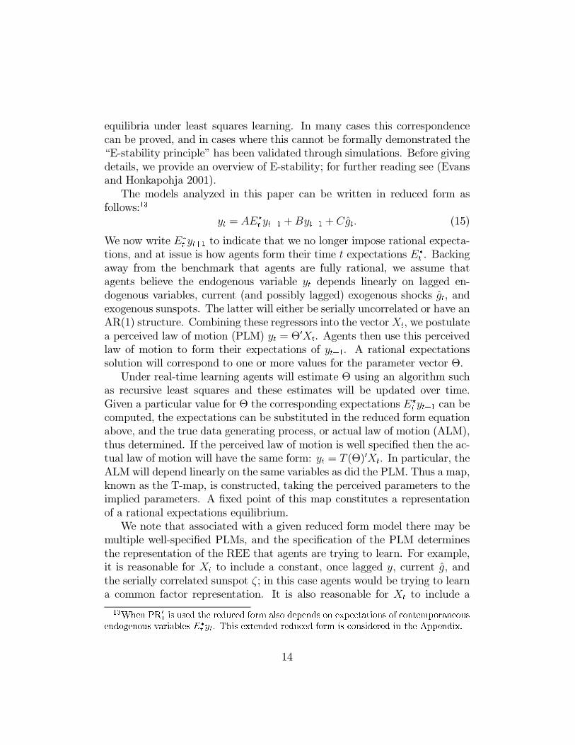
The models analyzed in this paper can be written in reduced form asfollows:13

yt = AE∗

tyt+1 +Byt−1 + Cgt. (15)

We now write E∗

tyt+1 to indicate that we no longer impose rational expecta-

tions, and at issue is how agents form their time t expectations E∗

t. Backing

away from the benchmark that agents are fully rational, we assume thatagents believe the endogenous variable yt depends linearly on lagged en-dogenous variables, current (and possibly lagged) exogenous shocks gt, andexogenous sunspots. The latter will either be serially uncorrelated or have anAR(1) structure. Combining these regressors into the vectorXt, we postulatea perceived law of motion (PLM) yt = Θ′Xt. Agents then use this perceivedlaw of motion to form their expectations of yt+1. A rational expectationssolution will correspond to one or more values for the parameter vector Θ.

Under real-time learning agents will estimate Θ using an algorithm suchas recursive least squares and these estimates will be updated over time.Given a particular value for Θ the corresponding expectations E∗

tyt+1 can be

computed, the expectations can be substituted in the reduced form equationabove, and the true data generating process, or actual law of motion (ALM),thus determined. If the perceived law of motion is well specified then the ac-tual law of motion will have the same form: yt = T (Θ)′Xt. In particular, theALMwill depend linearly on the same variables as did the PLM. Thus a map,known as the T-map, is constructed, taking the perceived parameters to theimplied parameters. A fixed point of this map constitutes a representationof a rational expectations equilibrium.

We note that associated with a given reduced form model there may bemultiple well-specified PLMs, and the specification of the PLM determinesthe representation of the REE that agents are trying to learn. For example,it is reasonable for Xt to include a constant, once lagged y, current g, andthe serially correlated sunspot ζ; in this case agents would be trying to learna common factor representation. It is also reasonable for Xt to include a

13When PR′

1is used the reduced form also depends on expectations of contemporaneous

endogenous variables E∗

tyt. This extended reduced form is considered in the Appendix.

14

constant, once and twice lagged y, current and once lagged g, and a mdsnoise term ξ; in this case agents would be trying to learn a general formrepresentation. Finally, we note that a fixed point of the T-map defines notjust an equilibrium, but also a representation of that equilibrium.

Once the T-map is obtained, the stability under learning of a particularrepresentation can be addressed as follows. Let the equilibrium represen-tation be characterized by the fixed point Θ∗, and consider the differentialequation

dΘ

dτ= T (Θ)−Θ. (16)

Notice that Θ∗ is a rest point of this ordinary differential equation. Therepresentation corresponding to the fixed point is said to be E-stable if it isa locally asymptotically stable equilibrium of (16). The E-stability principletells us that E-stable representations are locally learnable for Least Squaresand closely related algorithms. That is, if Θt is the time t estimate of thecoefficient vector Θ, and if Θt is updated over time using recursive leastsquares, then Θ∗ is a possible convergence point, i.e. locally Θt → Θ∗ if andonly if Θ∗ is E-stable. The intuition behind this principle is that a reasonablelearning algorithm, such as least squares, would gradually adjust estimatesΘt in the direction of the actual parameters T (Θt) that are generating thedata. For an E-stable fixed pointΘ∗ such a procedure would then be expectedto converge locally.

The above discussion has implicitly assumed a rest point Θ∗ that is locallyisolated. In this case it is locally asymptotically stable under (16) providedall eigenvalues of the Jacobian of T at Θ∗ have real parts less than one,and it is unstable if the Jacobian has at least one eigenvalue with real partgreater than one. Because we are studying sunspot equilibria, the set ofrest points of (16) may have unbounded continua as connected components.Along these components the T map will always be neutrally stable, and thuswill have at least one eigenvalue equal to unity.14 In this case we say asunspot equilibrium representation is E-stable if the Jacobian of the T -maphas eigenvalues with real part less than one, apart from unit eigenvaluesarising from the equilibrium connected components.

We consider separately the determinate and two indeterminate cases.

14The number of unit eigenvalues will be equal to the dimension of these components.

15

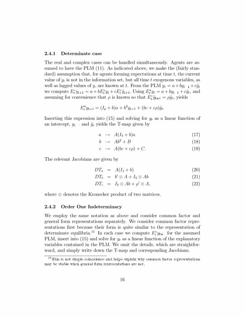
2.4.1 Determinate case

The real and complex cases can be handled simultaneously. Agents are as-sumed to have the PLM (11). As indicated above, we make the (fairly stan-dard) assumption that, for agents forming expectations at time t, the currentvalue of yt is not in the information set, but all time t exogenous variables, aswell as lagged values of y, are known at t. From the PLM yt = a+ byt−1+cgt

we compute E∗

tyt+1 = a+ bE∗

tyt+ cE∗

tgt+1. Using E∗

tyt = a+ byt−1+ cgt, and

assuming for convenience that ρ is known so that E∗

tgt+1 = ρgt, yields

E∗

tyt+1 = (I2 + b)a + b2yt−1 + (bc + cρ)gt.

Inserting this expression into (15) and solving for yt as a linear function ofan intercept, yt−1 and gt yields the T-map given by

a → A(I2 + b)a (17)

b → Ab2 + B (18)

c → A(bc+ cρ) + C. (19)

The relevant Jacobians are given by

DTa = A(I2 + b) (20)

DTb = b′ ⊗A+ I2 ⊗ Ab (21)

DTc = I2 ⊗ Ab+ ρ′ ⊗ A, (22)

where ⊗ denotes the Kronecker product of two matrices.

2.4.2 Order One Indeterminacy

We employ the same notation as above and consider common factor andgeneral form representations separately. We consider common factor repre-sentations first because their form is quite similar to the representation ofdeterminate equilibria.15 In each case we compute E∗

t yt+1 for the assumedPLM, insert into (15) and solve for yt as a linear function of the explanatoryvariables contained in the PLM. We omit the details, which are straightfor-ward, and simply write down the T-map and corresponding Jacobians.

15This is not simple coincidence and helps explain why common factor representationsmay be stable when general form representations are not.

16

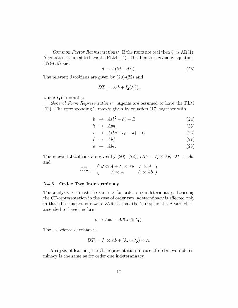
Common Factor Representations: If the roots are real then ζt is AR(1).Agents are assumed to have the PLM (14). The T-map is given by equations(17)-(19) and

d → A(bd+ dλi). (23)

The relevant Jacobians are given by (20)-(22) and

DTd = A(b+ I2(λi)),

where I2 (x) = x⊕ x.General Form Representations: Agents are assumed to have the PLM

(12). The corresponding T-map is given by equation (17) together with

b → A(b2 + h) +B (24)

h → Abh (25)

c → A(bc+ cρ + d) + C (26)

f → Abf (27)

e → Abe. (28)

The relevant Jacobians are given by (20), (22), DTf = I2 ⊗ Ab, DTe = Ab,and

DTbh =

(b′ ⊗ A+ I2 ⊗ Ab I2 ⊗ A

h′ ⊗A I2 ⊗ Ab

)

2.4.3 Order Two Indeterminacy

The analysis is almost the same as for order one indeterminacy. Learningthe CF-representation in the case of order two indeterminacy is affected onlyin that the sunspot is now a VAR so that the T-map in the d variable isamended to have the form

d → Abd+ Ad(λi ⊕ λj).

The associated Jacobian is

DTd = I2 ⊗ Ab+ (λi ⊕ λj)⊗A.

Analysis of learning the GF-representation in case of order two indeter-minacy is the same as for order one indeterminacy.

17

3 Results

We studied stability of general form and common factor sunspots in fivemodels, which differed only in the specification of the monetary policy rule,and the models are identified by the number of the corresponding policy ruleas given by equations (3)-(7). The models were analyzed using three differentcalibrations of the parameters in the IS-AS curves, as due to (Woodford1999), (Clarida, Gali, and Gertler 2000) and (McCallum and Nelson 1999);the relevant parameter values are given in Table 1 below.

Table 1: Calibrations

Author(s) φ λW 1/.157 .024

CGG 1 .3MN .164 .3

For convenience in interpreting the numerical results below we note that1/.157 � 6.3694 .

Also, each policy rule was analyzed both with and without lagged inflationin the AS equation (or Phillips curve). With pure Calvo pricing, and thusno inflation inertia in the AS equation, the discount rate β was set equalto .99 following W, CGG, and MN16. When lagged inflation was includedγ was set equal to one half, and we set β = 1, thereby imposing that thesum of the coefficients on inflation equals one. Finally, for all policy rules,the exogenous noise terms were taken to have damping parameter equal to.9. For each calibration (and for γ = 1 and .5), a lattice over the square(0, 10) × (0, 10) in policy space (απ, αx) was analyzed. For PR4 we alsocomputed results for several values of θ.

Some general results were found across all or most of the policy rulesand calibrations investigated, and are therefore worth summarizing beforepresenting more specific results in detail. Throughout this section we willuse “stable” to mean “stable under learning” as determined by E-stability.

1. In no case were General Form sunspot solutions stable.

16With γ = 1, the coefficient β modifying the expectations term in the AS equationresults from the optimal price setting behavior of the agents. However, more traditionalspecifications of the Phillips curve often specify this coefficient equal to one. For the caseγ = 1 and β = 0.99 we checked for robustness against γ = 1 and β = 1 and, except whereindicated, found little impact on our results.

18

2. In the determinate case the unique nonexplosive solution is usuallystable under learning: the exceptions are PR2, and with low γ, PR3, inwhich unstable cases exist.

3. The explosive case arises for PR2, and with low values of γ, for allpolicy rules.

4. Order two indeterminacy exists only for PR3 and is never stable.

5. Common Factor sunspot solutions exist17 for all forms of the policyrule, but they are only stable for PR3 and PR4.

6. Stable CF sunspots arise with γ = 0.5 as well as in the purely forwardlooking case γ = 1.

3.1 Policy Rule 1

As noted in Section 2, policy rule 1 has a natural variant, which we labelPR′

1. We summarize the results for PR1 and PR′

1 in separate subsectionsbelow.

3.1.1 PR1

For ease of exposition, we restate, at the beginning of each subsection, thespecification of the relevant policy rule. PR1 is given by

PR1 : it = αππt + αxxt.

PR1 with γ = 1 (i.e. no lagged inflation in the AS) has been analyzed by anumber of authors, including (Bullard and Mitra 2002) and (Honkapohja andMitra 2001). Bullard and Mitra found that the region in policy space corre-sponding to E-stability is precisely the region corresponding to determinacy;this result was obtained analytically and is independent of calibration.18 Be-cause of this result, Bullard and Mitra would recommend this policy rule if it

17In line with our earlier discussion, the statement “Common Factor sunspot solutionsexist” is now to be interpreted as asserting the existence of CF sunspot representationsbased on real roots.

18(Honkapohja and Mitra 2001) obtain the additional result, for γ = 1, that what wecall GF sunspot solutions are not stable. See their Proposition 4, which also covers PR3

for the case γ = 1.

19

were feasible. However, as discussed above, it is widely agreed that currentvalues of inflation and GDP are not available to policymakers. We includeresults for this policy rule primarily because it serves as a useful benchmark.We find that the result of Bullard and Mitra is robust to the inclusion ofinflation inertia in the Phillips curve: in all cases investigated, determinacyimplies stability under learning. In addition, when the model is indetermi-nate no solutions are stable, including CF sunspot solutions.

An example lattice is plotted in Figure 1 for the Woodford calibrationwith γ = 1. Here and in all figures containing lattice plots, each latticepoint is marked with a symbol indicating properties of the associated steadystate: lattice points associated with determinate steady states are markedwith an ‘×’; lattice points associated with indeterminate steady states and forwhich common factor representations exist (i.e. there exist at least two realeigenvalues) are marked with a ‘∗’, and lattice points associated with indeter-minate steady states for which no common factor representations exist (i.e.there exists at most one real eigenvalue) are marked with a ‘·’. Also, if thereexists a stable representation associated with the steady state, the symbolmarking the lattice point is circled. CF sunspots exist for all indeterminatecases, a finding that extends to the other calibrations with γ = 1.

Figure 1 Here

Figure 2 shows the regions of determinacy and indeterminacy pertainingto the CGG calibration with γ = .5. The main result that all CF and GFsunspots are unstable still holds, but the region of determinacy is altered andhere it is no longer the case that CF sunspots always exist. The failure ofCF sunspots to exist seems to depend principally on the inertial term in thePhillips curve. When γ is set equal to one, all indeterminate steady statessupport common factor sunspots. The MN calibration yields much the samepicture as the CGG calibration. Note that the range of policy parametersdisplayed does not necessarily coincide with the 10× 10 grid, and also variesacross figures; this was done to emphasize features particular to given figures.

Figure 2 Here

One further result of interest (not shown) is that sufficiently low values ofγ > 0 together with passive response to inflation (low απ) can yield theexplosive case.

20

Under our information assumptions, when policymakers use PR1 they ef-fectively have an information advantage relative to private agents. This isbecause policymakers are conditioning policy on contemporaneous endoge-nous variables, which are assumed not available to private agents when theirforming expectations. This information asymmetry does not arise under PR′

1

to which we now turn.

3.1.2 PR′

1

PR′

1 is given byPR′

1 : it = απE∗

t πt + αxE∗

t xt.

This policy can be thought of as a contemporaneous rule that is feasible evenif current values of the endogenous variables πt and xt are not known at timet. We continue to make the assumption that all t-dated exogenous variablesand all lagged variables are observed prior to expectations formation. Asdiscussed further in Section 3.3, below, we are also making the homogeneousexpectations assumption that policymakers and private agents form expec-tations in the same way. In contrast to our PR1, under PR

′

1 policy makersand private agents are treated as having the same information set.

In a rational expectations equilibrium Etπt = πt and Etxt = xt. Thisimplies that the REE, their representations, and the regions of determinacy,indeterminacy, and explosiveness will be precisely as they were under PR1.However, out of equilibrium, agents may make errors when forecasting cur-rent values of the endogenous variables. In particular, because learningdynamics are in part determined by out of equilibrium behavior, the stabil-ity properties of the model under PR′

1 may be different than under PR1: seethe Appendix for details on how the learning analysis is altered.

(Bullard and Mitra 2002) analyzed PR′

1, though with a slightly differentinterpretation of the timing structure: they assume that expectations formedat t use only information available at time t− 1. Although this differs fromour assumption that exogenous variables at time t are part of the informationset, it can be verified that the E-stability conditions are identical for the twoinformation assumptions. Bullard and Mitra show, analytically, that theirresults for PR1 hold also for PR′

1. In particular, the regions of determinacyare the same for both policy rules, and, for each policy rule, a steady stateis stable under learning if and only if it is determinate.

We obtain the same correspondence and find that it also extends to thestability of sunspot solutions. We have already noted that the regions of de-

21

terminacy, indeterminacy, and explosiveness are the same for PR1 and PR′

1.In addition, our numerical analysis indicates that for all parameter combi-nations considered, all determinate steady-states are stable under learning,and no stable indeterminacies exist. Our results thus tend to reinforce thoseof (Bullard and Mitra 2002), who in consequence recommend Taylor rules ofthe form PR′

1 with απ > 1.

3.2 Policy Rule 2

PR2 is given byPR2 : it = αππt−1 + αxxt−1.

PR2, with γ = 1, was also studied by Bullard and Mitra. Numerically, andusing the Woodford calibration, they found that, unlike PR1, there weredeterminate cases for which the REE was not stable under learning. Theyconcluded that policy rules dependent on lagged output gap and inflation maynot be advisable because agents may fail to coordinate on the equilibriumeven though it is unique. We find that this result is robust to the calibrationsconsidered here and extends to the specification with inertial inflation in thePhillips curve. Figure 3 gives an example plot using the CGG calibrationand with γ = .5. In this Figure, lattice points left unmarked correspond toexplosive steady states.

Figure 3 Here

Aggressive response to output gap and inflation may yield explosive steadystates. In fact, using the Woodford calibration one obtains that even passiveresponse to output gap (αx > .35), together with a Taylor rule απ > 1, canyield an explosive steady state. In the indeterminate region CF representa-tions exist but they are not stable.

3.3 Policy Rule 3

PR3 is given byPR3 : it = απE

∗

t πt+1 + αxE∗

t xt+1.

Before giving the results we discuss the interpretation of this rule under learn-ing. Under least squares learning private agents are assumed to recursivelyestimate the parameters of their PLM and use the estimated forecasting

22

model to form the expectations E∗

t πt+1 and E∗

t xt+1 that enter into their de-cisions as captured by the IS and AS curves. Under PR3 and PR4 forecastsalso enter into the policy rule. Because we are now relaxing the rational ex-pectations assumption, one can in principle distinguish between the forecastsof the private sector, which enter the IS and AS curves, and the forecasts ofthe Central Bank, which enter policy rule PR3 or PR4. We will instead adoptthe simplest assumption for studying stability under learning, which is thatthe forecasts for the private sector and the Central Bank are identical. Thiscan either be because private agents and the Central Bank use the same leastsquares learning scheme, or it could be because one group relies on the others’forecasts. In the latter case, for example, the Central Bank might be settinginterest rates as a reaction to private sector forecasts, as in (Bernanke andWoodford 1997) or (Evans and Honkapohja 2003a). The homogeneous ex-pectations assumption was also adopted in (Bullard and Mitra 2002).19 Sincewe are searching for stable sunspot equilibria, the homogeneous expectationsassumption appears to give the greatest likelihood for finding them.

We now turn to the results. For policy rule PR3, under the calibrationsstudied, all determinate steady states are stable and no explosive steadystates are observed.20 However, in contrast to PR1 and PR2, policy rulePR3 can exhibit stable sunspots, and the region of stability may includeeconomically reasonable parameter values. This result corroborates and ex-tends those of (Honkapohja and Mitra 2001), who showed the existence ofstable noisy K-state Markov sunspots for this policy rule. We discuss therelationship of our results to theirs below.

For the W and CGG calibrations, and for both values of γ, stable commonfactor representations exist. For the CGG calibration the region of stabilityrequires aggressive (“active”) policy response to both the output gap and toinflation, i.e. απ > 1 and αx > 1. Although the “Taylor principle” specificallyrecommends απ > 1, output gap responses of αx > 1 might be considered tooaggressive. However, using the W calibration, stable CF sunspots arise withvery plausible policy settings, including in particular the benchmark choiceαπ = 1.5 and αx = 0.5 discussed by (Taylor 1993). (For the MN calibrations,stable CF representations exist, but not in the 10 × 10 benchmark policy

19The implications of heterogeneous expectations in the context of the New Keyen-sian monetary model is examined in (Honkapohja and Mitra 2002). This issue is furtherdiscussed in (Evans and Honkapohja 2003a)

20As noted earlier, in case of very low γ, unstable determinacy and explosive steadystates are present.

23

space: αx > 12 yields stable sunspots).Consider Figure 4, showing the regions of stability of CF representations

for the Woodford calibration with γ = 1.21

Figures 4, 5 Here

For this calibration stable CF sunspots appear for large regions of plausiblepolicy parameters. For the Woodford calibration, the results are almost asdramatic for the case γ = 0.5, as can be seen in Figure 5. Recall that whenwe set γ = 1 we also set β = 0.99 in line with W, CGG and MN, whereas forthe case γ = 0.5 we set β = 1, as in (Fuhrer and Moore 1995). The existenceof stable CF sunspots does not depend on the choice of β, but the preciseregion is sensitive to this choice for PR3: for β < 1 (and either value of γ)the region of stable CF sunspots includes regions of part of the passive policyregion απ < 1.

We now relate these results to those found elsewhere in the literature.(Bullard and Mitra 2002) studied this model with γ = 1, and showed thatall determinate equilibria were stable under learning. Our findings indicatethat this result extends to models that include lagged inflation in the AScurve. Bullard and Mitra also found that for indeterminate steady-states theMSV solution22 may be stable, and pointed out that whether agents couldlearn sunspots in this case was an open question. Clearly the answer to thisquestion is a resounding yes. In particular, common factor representationscan be thought of as MSV representations together with serially correlatedsunspots, and we have found that these sunspots may be stable.

(Honkapohja andMitra 2001) studied this model, with γ = 1, and demon-strated that finite state “resonance frequency” sunspots exist and are stablefor a region of the parameter space. These solutions take the form

yt = cgt + dst

where st is a K × 1 vector representing a K-state Markov process withtransition probabilities that satisfy particular conditions sometimes called“resonant frequency conditions.” This result is consistent with and, in fact,suggestive of ours.

21In Figures 4 and 5, unmarked lattice points indicate order two indeterminacy.22By MSV solution is meant a solution that depends on a minimal number of state

variables. For a discussion see (McCallum 1983) and (Evans and Honkapohja 2001).

24

In (Evans and McGough 2002b) we show that there is an intimate linkbetween CF representations and finite-state sunspots in univariate models.For the current model with γ = 1 our solutions (14) satisfy b = 0 and thustake the form

yt = cgt + dζt,

where, in the case of order-one indeterminacy, ζt is an AR(1) process ζt =λiζt−1 + εt.

23 Particular choices of the mds εt yield solutions of the formyt = cgt + dst with the required transition probabilities. When 0 < γ < 1our CF solutions take the form

yt = byt−1 + cgt + dζt,

where now b �= 0. The condition that the AR(1) coefficient is λi, for i = 2, 3,i.e. equal to a critical eigenvalue, is the resonant frequency condition forCF solutions. Our PR3 result can thus be thought of as a generalization ofthe Honkapohja-Mitra finding: we extend the economic model to the caseγ < 1, in which the model has backward looking components, and we exhibitand study the more general representations taking the form of CF sunspotsolutions.

(Evans and Honkapohja 2003d) studied optimal discretionary policy inthe model (1)-(2), with γ = 1, and advise an interest rate designed specif-ically to offset any destabilizing forward looking behavior of agents. Theirrecommended interest rate rule takes the form

it = δπE∗

t πt+1 + δxE∗

t xt+1 + δggt,

where δπ = 1 + λβφ−1(α+ λ2)−1, δx = φ−1, δg =(φ−1, λφ−1(α + λ2)−1

)and

α ≥ 0 parameterizes the weight placed by the policy maker on output relativeto inflation volatility. Note that optimal policy requires a dependence on gtas well as on inflation and output forecasts, but the presence of this term doesnot affect determinacy or stability.24 (Evans and Honkapohja 2003d) showthat this rule is invariably determinate and that the REE is always E-stableand hence stable under least squares learning. This rule is recommended in

23If εt is white noise then ζtis a stationary AR(1) process since |λi| < 1. For general

mds εt the process ζtneed not be stationary, but ζ

twill be nonexplosive in conditional

mean (and ζtcan be expressed as an absolutely summable infinite moving average process

in εt−s).24In the reduced form, only the coefficient C of gt is affected. This does not affect the

E-stability conditions or the conditions for determinacy, as can be seen from the Appendix.

25

preference to other interest rate policies, such as fundamentals based rulesdepending only on gt, which they show to be unstable under learning eventhough they are consistent with the REE corresponding to optimal discre-tionary policy.

The size of the stable determinacy region surrounding this policy dependson the structural parameters. We investigated this point by analyzing ninelattices over the square (0, 10)×(0, 10) in policy space (απ, αx) correspondingto all permutations of λ ∈ {.024, .3, 1} and φ ∈ {.164, 1, 1/.157}, with γ = 1.In each case there are qualitatively similar regions: stable determinacy (Fig-ure 4, region A) lies at least part way along the horizontal axis for απ > 1and is bounded above by a downward sloping line, unstable indeterminacy(Figure 4, region B) lies at least part way along the vertical axis for απ < 1and is bounded on the right by a downward sloping line. The area of stableCF sunspots (Figure 4, region C) is the region that remains. However, quan-titatively we find the following: first, for fixed λ, as φ gets smaller, the regionof stable indeterminacy shifts up, replaced by stable determinacy, and theregion of unstable indeterminacy appears unaffected; second, for fixed φ, as λgets smaller, the region of stable indeterminacy shifts up slightly, replaced bystable determinacy, and again, the region of unstable indeterminacy appearsunaffected.25

The existence of stable sunspots in part of the parameter space pro-vides an important caveat to following the advice of (Evans and Honkapohja2003d). Policy makers may think the economy is in a determinate and stableregion of its parameter space and thus that agents will learn the intendedequilibrium; however, if policy makers are wrong about the values of the keyparameters λ and φ, agents may instead coordinate on an inferior sunspotequilibrium.

Stability and determinacy respect small continuous movements in para-meter values, and thus for any particular calibration, the Evans-Honkapohjarule will work well locally. (Evans and Honkapohja 2003d) also show that

25In the case γ = 1 analytic stability results are possible. We find that providedαx �= 1/φ then necessary and sufficient conditions for the existence of stable sunspots aregiven by

λ (απ − 1) + αx (1− β) > 0

λ (απ − 1) + αx (1 + β) > 2(1 + β)/φ.

These are precisely the same restrictions obtained by (Honkapohja and Mitra 2001) fornoisy finite-state Markov sunspot solutions.

26

the system under learning remains locally stable even when policy makersare simultaneously updating estimates λ and φ.26 However, numerical re-sults suggest that the margin for error available to policy makers when at-tempting to follow the Evans-Honkapohja rule, can depend critically on thestructural parameters. As an extreme, but perhaps not implausible example,we obtained results for λ = 1, φ = 6.3694, and γ = 1. The value φ is theone used in the W calibration, and λ = 1 is within the range of estimatesfrom the literature mentioned on p. 170, footnote 32, in (Clarida, Gali, andGertler 2000).

Figure 6 Here

In Figure 6 we see that a triangle of stable determinacy exists, but it isbordered by unstable indeterminacy on the left, and, even more ominously,by stable indeterminacy on the right. We conclude that in some cases learn-able sunspots abound in regions not far from those corresponding to optimalpolicy. Our findings also import a more general warning: simply following aTaylor rule with aggressive response to expected inflation is not necessarilystabilizing for the economy. This warning is emphasized for the parame-ter values used in Figure 6. Note that even for αx = 0, stable sunspotsexist if απ > 1.7. In contrast, if the CGG values are correct then the Evans-Honkapohja rule is quite robust.

3.4 Policy Rule 4

PR4 is given by

PR4 : it = θit−1 + (1− θ)απE∗

tπt+1 + (1− θ)αxxt,

where θ > 0. This policy rule is of particular interest in part because it isthe form of the rule specifically considered in part IV of (Clarida, Gali, andGertler 2000). Furthermore, the issue of inertia in policy rules, captured byθ > 0, has been discussed extensively in the literature. (Clarida, Gali, andGertler 2000) use the value θ = 0.68 based on (quarterly) estimates from thepre-Volker period, but there is no agreement that this is an appropriate value.

26That is, locally there is asymptotic convergence both of structural parameter estimatesto their true values λ, φ and forecasts E∗

txt+1, E

∗

tπt+1 to their RE values. Hence locally

the economy converges to the REE corresponding to optimal discretionary policy.

27

On the one hand (Rudebusch 2002) argues that the usual empirical evidencefor monetary policy inertia may well be illusory and that the true value of θmay be zero or small. On the other hand (Rotemberg and Woodford 1999)have argued that θ > 1 with απ > 0 may be close to optimal. Interest raterules with θ > 1 are often called “superinertial.”

(Honkapohja and Mitra 2001) analyzed PR4 numerically, for γ = 1, andfound that for the CGG calibration of λ and φ and with their estimated valuesof αx, απ and θ for the pre-Volker era, the sunspot solutions that we callgeneral form representations were unstable under learning. We confirm thisresult and we find also that although CF-sunspot solutions do exist, they arenot stable under learning. Figure 7 shows the results for the CGG calibrationof λ and φ with θ = 0.68: in the 10 × 10 policy grid for (αx, απ), thereare no stable CF sunspots, while all determinate steady states are learnable.Furthermore, these results are robust both to the inclusion of lagged inflationin the AS curve, 0 < γ < 1, and to the magnitude of 0 < θ < 1.

Figure 7 Here

However, as with PR3, we find that there are many cases in which stableCF sunspots exist, and the location of this region in policy space is verysensitive to the values of structural parameters assumed. Even with the CGGcalibration for λ and φ and with θ = 0.68, there exist stable CF sunspots forsufficiently large values of απ. Furthermore, for other values of λ and φ wefind that the possibility of stable CF sunspots needs to be taken seriously.For example, for the values φ = 1/.157 and λ = 1 examined earlier, stable CFsunspots exist for passive responses to output gap, and aggressive responsesto inflation; further, as θ gets small, the response to inflation required forstability becomes reasonably valued: see Figure 8 in which we set θ = 0.1.A very similar figure is obtained in case γ = .5; in particular, the presenceof inflation inertia in the AS curve does not preclude stable CF sunspots atreasonable parameter values.

Figure 8 Here

Because the region of stable indeterminacy depends on the structural pa-rameters φ and λ, as well as the interest rate smoothing term θ, we againtest the robustness of our results to alternative calibrations. We analyzed27 lattices over the square (0, 10) × (0, 10) in policy space (απ, αx) corre-sponding to all permutations of λ ∈ {.024, .3, 1}, φ ∈ {.164, 1, 1/.157}, and

28

θ ∈ {.05, .5, .9}. For this exercise we set γ = 1. In general, there are two re-gions of indeterminacy: an unstable region along the vertical axis for απ < 1:see Figure 8, Region B; and a triangular region of stable CF sunspots in thesoutheast corner: see Figure 8, Region C; the remaining region correspondsto stable determinacy: see Figure 8, Region A. We find that as φ and λget smaller, and as θ gets larger, the region of stable indeterminacy shiftsto the right, replaced by stable determinacy. The unstable region appearsunaffected.

One conclusion that emerges from this analysis is that while stable sunspotsdo exist under PR4 for sufficiently aggressive responses to expected inflation,the policy maker may hedge against the danger, which depends on the truevalues of λ and φ, by setting the smoothing term 0 < θ < 1 to be fairlyhigh.27

Finally, it is of interest to examine the case of superinertial rules withθ > 1. To remain consistent with the superinertial rules already in theliterature, we modify PR4 so as to ensure that the coefficients on expectedinflation and current output gap are positive:

PR′

4 : it = θit−1 + χπE∗

t πt+1 + χxxt.

We examined equilibria corresponding to a 10×10 lattice over (χπ, χx) policyspace, and for θ = 1.1 and 2, and γ = 1 and .5. For the W, CGG, and MNcalibrations, this rule performed well; for all permutations of θ and γ and overthe entire benchmark lattice the corresponding steady states were stable anddeterminate. However, stable indeterminacy was found for the alternativecalibration φ = 1/.157, and λ = 1: see Figure 9. The existence of thesestable sunspots is robust to the permutations of θ and γ.

Figure 9 Here

3.5 Discussion

Sunspot equilibria are stable under learning only for Taylor-type policy rulesthat depend on forecasts of future inflation, and only for certain solutionrepresentations that we call “common factor” representations. However, for

27(Bullard and Mitra 2003) consider in detail the impact of interest rate inertia ondeterminacy and stability of MSV solutions, and reach the same conclusion.

29

such forward looking rules stable CF sunspots are abundant. The location ofthe region of stable sunspot solutions depends on the structural parameters φand λ in the IS and AS curves. When these parameters are large, the regionof stable CF sunspots, in the policy parameter space, includes realistic valuesfor feedback coefficients in the interest rate rule. In particular, following theTaylor principle απ > 1 is not sufficient to avoid stable CF sunspots, even ifthe output feedback αx is small. Given uncertainty about the true values forφ and λ, the possibility of stable sunspots appears to be of genuine concern,and the possibility, in the indeterminate case, of all solutions being unstableis equally troubling.

Stable CF sunspot solutions can arise even if there are backward lookingcomponents to inflation and even if there is inertia (interest rate smooth-ing) in the monetary policy rule. This possibility had not been previouslyrecognized in the literature. Interest rate inertia does, however, increase theregion of stable determinacy relative to the benchmark policy square.

In general, inertia, or backward looking behavior, might be expected toreduce the risk of indeterminacy (i.e. reduce the proportion of the benchmarkparameter space corresponding to indeterminate steady states). While wehave demonstrated that inertial components in the AS curve and policy ruledo not overturn our main results, it is possible that inertia in the IS curve— specifically, a dependence on lagged output gap, justified, say, by habitformation — may have an important impact. Investigation of this issue willreceive a high priority in our future research.28

Our study of interest rate inertia focussed on interest rate rule PR4. Itwould also be useful to investigate the influence on the regions of determinacyand stability of an interest rate smoothing term in rules PR1 — PR3. Werestricted attention to the specification of these rules without the inertialterm for expedience. However our preliminary investigations indicate thatwhile the location and relative size of the regions of determinacy and stabilityare altered somewhat, the presence of interest rate inertia in policy rules PR1

— PR3 does not, in general, change our central results. This is also an issuethat we intend to investigate more thoroughly in future work.

28In principle, stability under learning can be investigated using large scale macro-econometric models; see, for example, (Garratt and Hall 1997). Our techniques could beextended to study the stability of CF sunspot solutions in such models as well as to alarger class of policy rules.

30

4 Conclusion

This paper has examined the question of whether macroeconomic fluctua-tions, taking the form of coordination on extraneous exogenous variables,are likely to emerge under adaptive learning when the economy is character-ized by New Keynesian IS-AS equations and monetary policy follows a formof Taylor rule. Both purely forward-looking and hybrid, partly backward-looking inflation equations were examined. We have emphasized that thepossibility of “sunspot equilibria” that are stable under adaptive learningdepends critically on the representation of the solution, i.e. on the econo-metric specification used by agents when they estimate and update theirforecasting model.

In many cases stationary sunspot equilibria can be represented either as“general form” VARs, driven by serially uncorrelated sunspots, or as “com-mon factor” sunspot solutions, in which the extraneous sunspot variablesare autoregressive processes with resonant frequency coefficients. Commonfactor sunspots generalize finite state Markov sunspots, which were an earlyfocus in the sunspot literature and which have recently been shown to yieldthe possibility of stable sunspots in purely forward looking linear models.In the New Keynesian model, we find that common factor sunspots can in-deed be stable under learning, in many cases, even though the general formsolutions with serially uncorrelated sunspots are not.

In particular, Taylor-type interest rate rules that depend on forecasts offuture inflation can generate stable common factor sunspot solutions, andthis risk is particularly high when there are strong IS and AS effects. Thispossibility arises even if the AS equation includes backward looking com-ponents and the interest rate rule includes inertia. This result is deeplytroubling since monetary policy is often viewed as forward looking. If thestructural model and its key parameters are known, or can be estimated fairlyprecisely, then an appropriately designed forward looking policy can delivera stable determinate equilibrium (indeed an optimal stable equilibrium) andthe sunspot problem will not arise. However, for some structural parametersthe margin of error is small and the impact of an error is great. In contrast,policy rules depending on forecasts of current output and inflation do notappear to be subject to these difficulties.

31

AppendixTo illustrate the details of the technique we focus on the policy rule PR1

given by (3). In this case

H =

1 + φαx φαπ 0 −1 0−λ 1 β(γ − 1) 0 −10 1 0 0 00 0 0 ρg 00 0 0 0 ρu

and F =

1 φ 0 0 00 βγ 0 0 00 0 1 0 00 0 0 1 00 0 0 0 1

Order one indeterminacy. This occurs when |λ1| > 1 and the re-maining eigenvalues have norm less than one. Notice this implies λ1 is real;however λi for i > 1 may be complex. For reasons discussed above, in the in-determinate case, we only consider real eigenvalues. To obtain a nonexplosivesolution, we require z1t = 0, and ε1t + w1t = 0.

General Form Representations: A general form representation is theusual recursive system describing the equilibrium and is characterized by asunspot that forms a martingale difference sequence. Fix i = 2 or 3. We maythen use the nonexplosiveness condition z1t = 0 together with the equation

zit = λizit−1 + wit + εit

to obtain the following representation.

yt = (S11

i )−1(

0 −S13

λiSi1 λiS

i2 − Si3

)yt−1 + (S11

i )−1(

0 00 λiS

i3

)yt−2

−(S11

i )−1S14

i gt + (S11

i )−1(

0 0λiS

i4 λiSi5

)gt−1

+(S11

i )−1(

01

)wit + (S11

i )−1(

01

)εit.

The identities

wit =((FS)i4, (FS)i5

)wt

ξit =(Si1, Si2

)εt

wt = gt − ρgt−1

may be used to place this representation in the form given in the text.

32

Common Factor Representations: Again assume |λ1| > 1 and the remain-ing eigenvalues have norm less than one. Let εt be a mds with ε1t + w1t = 0.Pick i = 2 or 3. The REE associated to εt must satisfy the equation

zit = λizit−1 + wit + εit,

orzit = (1− λiL)

−1(wit + εit).

We interpret the noise term on the right to be a sunspot ζt and thus writezit = ζt with

ζt = λiζt−1 + wit + εit.

Combining this with the restriction z1t = 0 yields two common factor repre-sentations of the form

yt = −(S11

i )−1(

0 S13

0 Si3

)yt−1 − (S11

i )−1S14

i gt + (S11

i )−1(

01

)ζt.

Order two indeterminacy.General Form Representations: Now all eigenvalues are in the unit circle

and thus there is no concern over the nonexplosiveness restriction. Pick realeigenvalues λi, and λj. We can write

(zitzjt

)= (λi ⊕ λj)

(zit−1zjt−1

)+

(wit

wjt

)+

(εitεjt

).

This can be rearranged to yield the following representation:

yt = (Si1j )

−1

(λiS

i1 λiSi2 − Si3

λjSj1 λjS

j2 − Sj3

)yt−1 + (Si1

j )−1

(0 λiS

i3

0 λjSj3

)yt−2

−(Si1j )

−1Si4j gt + (Si1

j )−1

(λiS

i4 λiSi5

λjSj4 λjS

j5

)gt−1

+(Si1j )

−1

(wit

wjt

)+ (Si1

j )−1

(εitεjt

).

Common Factor Representations: Again, pick real eigenvalues λi, and λj.Then we may define the VAR sunspot

ζt = (λi ⊕ λj)ζt−1 +

(wit

wjt

)+

(εitεjt

).

33

The resulting CF representation has the form

yt = −(Si1j )

−1

(0 Si3

0 Sj3

)yt−1 − (Si1

j )−1Si4

j gt + (Si1j )

−1ζt.

Learning. For PR1 the reduced form is(xt

πt

)= AEt

(xt+1

πt+1

)+B

(xt−1

πt−1

)+ C

(gtut

),

where

A =

(δ φ(1− απβγ)δλδ βγ + λφ(1− απβγ)δ

)

B =

(0 −φαπβ(1− γ)δ0 β(1− γ)− λφαπβ(1− γ)δ

)

C =

(δ −φαπδλδ 1− λφαπδ

),

and δ = (1 + φ(αx + λαπ))−1.

For PR′

1 the reduced form is(xt

πt

)= AE∗

t

(xt+1

πt+1

)+B

(xt−1

πt−1

)+ C

(gtut

)+DE∗

t

(xt

πt

)

where

A =

(1 φλ βγ + λφ

)

B =

(0 00 β(1− γ)

)

C =

(1 0λ 1

)

D =

(−φαx −φαπ

−λφαx −λφαπ

)

For all of our policy rules the CF-PLM is given by

yt = a+ byt−1 + cgt + dζ tζt = λiζt−1 + εt.

34

The associated T-map is

a → (A(I2 + b) +D)a

b → Ab2 +Db+B

c → A(bc+ cρ) +Dc+ C

d → A(bd+ dλi) +Dd

The relevant Jacobians are given by

DTa = A(I2 + b) +D

DTb = b′ ⊗ A+ I2 ⊗Ab+ I2 ⊗D

DTc = I2 ⊗Ab+ ρ′ ⊗ A+ I2 ⊗D

DTd = Ab+ λi ⊗ A+D.

The E-stability conditions are that the real part is less than 1 for every eigen-value of DTi, i = a, b, c, d. The general form case can be handled similarly.

35

References

B�������, B., ��� M. W������� (1997): “Inflation Forecasts and Mon-etary Policy,” Journal of Money, Credit, and Banking, 24, 653—684.

B���, J., ��� K. M���� (2002): “Learning About Monetary PolicyRules,” Journal of Monetary Economics, 49, 1105—1129.

(2003): “Determinacy, Learnability and Monetary Policy Inertia,”Working paper, Federal Reserve Bank of St. Louis.

C�����, R., J. G��, ��� M. G����� (1999): “The Science of MonetaryPolicy: A New Keynesian Perspective,” Journal of Economic Literature,37, 1661—1707.

(2000): “Monetary Policy Rules and Macroeconomic Stability: Ev-idence and Some Theory,” Quarterly Journal of Economics, 115, 147—180.

D� ������ , G., ��� G. N������ (2001): “Expectations Coordinationon a Sunspot Equilibrium: an Eductive Approach,” Macroeconomic Dy-

namics, 7, 7—41.

E��� , G. W., ��� R. G� ����� (2003): “Coordination on Saddle PathSolutions: the Eductive Viewpoint — Linear Univariate Models,” Macro-

economic Dynamics, 7, 42—62.

E��� , G. W., ��� S. H��������� (1994): “On the Local Stability ofSunspot Equilibria under Adaptive Learning Rules,” Journal of Economic

Theory, 64, 142—161.

(2001): Learning and Expectations in Macroeconomics. PrincetonUniversity Press, Princeton, New Jersey.

(2003a): “Adaptive Learning and Monetary Policy Design,” Journalof Money, Credit and Banking, forthcoming.

(2003b): “Existence of Adaptively Stable Sunspot Equilibria near anIndeterminate Steady State,” Journal of Economic Theory, 111, 125—134.

(2003c): “Expectational Stability of Stationary Sunspot Equilibriain a Forward-looking Model,” Journal of Economic Dynamics and Control,28, 171—181.

36

(2003d): “Expectations and the Stability Problem for Optimal Mon-etary Policies,” Review of Economic Studies, forthcoming.

E��� , G. W., S. H���������, ��� R. M������ (2001): “StableSunspot Equilibria in a Cash in Advance Economy,” mimeo.

E��� , G. W., S. H���������, ��� P. R���� (1998): “Growth Cycles,”American Economic Review, 88, 495—515.

E��� , G. W., ��� B. M�G��� (2002a): “Indeterminacy and the Sta-bility Puzzle in Non-Convex Economies,” mimeo.

(2002b): “Stable Noisy K-state Sunspots,” mimeo,http://darkwing.uoregon.edu/∼gevans/.

(2003): “Stable Sunspot Solutions in Models with PredeterminedVariables,” Journal of Economic Dynamics and Control, forthcoming.

F�����, R. E., ��� J.-T. G� (1994): “Real Business Cycles and theAnimal Spirits Hypothesis,” Journal of Economic Theory, 63, 42—72.

F����, J., ��� G. M���� (1995): “Inflation Persistence,” Quarterly

Journal of Economics, 110, 127—159.

G��, J., ��� M. G����� (1999): “Inflation Dynamics: A StructuralEconometric Approach,” Journal of Monetary Economics, 44, 195—222.

G������, A., ��� S. H� (1997): “E-Equilibria and Adaptive Expec-tations: Output and Inflation in the LBS Model,” Journal of Economic

Dynamics and Control, 21, 1149—1171.

G� �����, R. (1992): “An Exploration of the Eductive Justifications ofthe Rational-Expectations Hypothesis,” American Economic Review, 82,1254—1278.

H���������, S., ��� K. M���� (2001): “Are Non-FundamentalEquilibria Learnable in Models of Monetary Policy?,” Working paper,www.valt.helsinki.fi/RAKA/seppo.hmtl.

(2002): “Performance of Monetary Policy with Internal CentralBank Forecasting,” manuscript, www.valt.helsinki.fi/RAKA/seppo.hmtl.

37

H�����, P. (1992): “Interest Rate Control and Nonconvergence to RationalExpectations,” Journal of Political Economy, 100, 776—800.

H�����, P., ��� R. P. M�A��� (1992): “Animal Spirits,” American Eco-

nomic Review, 82, 493—507.

M�C��, B. (1983): “On Nonuniqueness in Linear Rational Expecta-tions Models: An Attempt at Perspective,” The Journal of Monetary

Economics, 11, 134—168.

M�C��, B. T. (1999): “Issues in the Design of Monetary Policy Rules,”in (Taylor and Woodford 1999), chap. 23, pp. 1483—1530.

M�C��, B. T., ��� E. N� �� (1999): “Performance of OperationalPolicy Rules in an Estimated Semi-Classical Model,” in (Taylor 1999), pp.15—45.

R��������, J. J., ��� M. W������� (1999): “Interest-Rate Rules inan Estimated Sticky Price Model,” in (Taylor 1999), pp. 55—119.

R��� ��, G. D. (2002): “Term Structure Evidence on Interest RateSmoothing and Monetary Policy Inertis,” Journal of Monetary Economics,49, 1161—1187.

S��� ��, L. E. O., ��� M. W������� (1999): “Implementing OptimalPolicy through Inflation-Forecast Targeting,” Working paper.

T����, J. (1993): “Discretion versus Policy Rules in Practice,” Carnegie-

Rochester Conference Series in Public Policy, 39, 195—214.

(ed.) (1999): Monetary Policy Rules. University of Chicago Press,Chicago.

T����, J., ��� M. W������� (eds.) (1999): Handbook of Macroeco-

nomics, Volume 1. Elsevier, Amsterdam.

W�������, M. (1990): “Learning to Believe in Sunspots,” Econometrica,58, 277—307.

(1999): “Optimal Monetary Policy Inertia,” The Manchester School,

Supplement, 67, 1—35.

38

(2003): Interest and Prices: Foundations of a Theory of Monetary

Policy. Princeton University Press, Princeton, NJ.

39

0 0.2 0.4 0.6 0.8 1 1.2 1.4 1.6 1.8 20

0.5

1

1.5

2

2.5

3Figure 1: Policy Rule 1, Woodford Calibration, γ=1

απ

α x

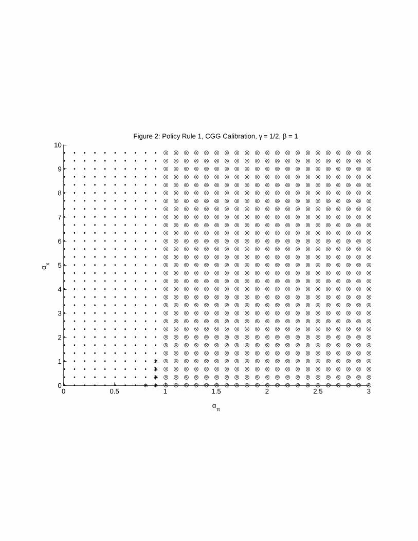
0 0.5 1 1.5 2 2.5 30

1

2

3

4

5

6

7

8

9

10Figure 2: Policy Rule 1, CGG Calibration, γ = 1/2, β = 1

απ

α x

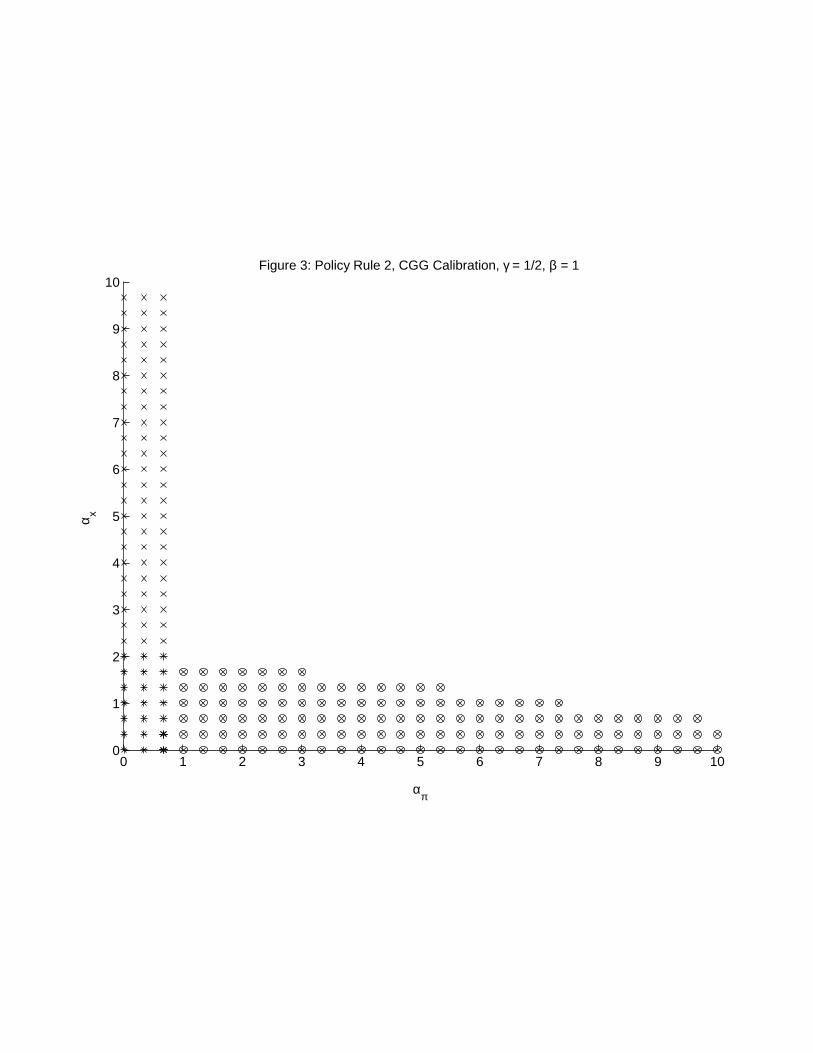
0 1 2 3 4 5 6 7 8 9 100

1

2

3

4

5

6

7

8

9

10Figure 3: Policy Rule 2, CGG Calibration, γ = 1/2, β = 1

απ

α x

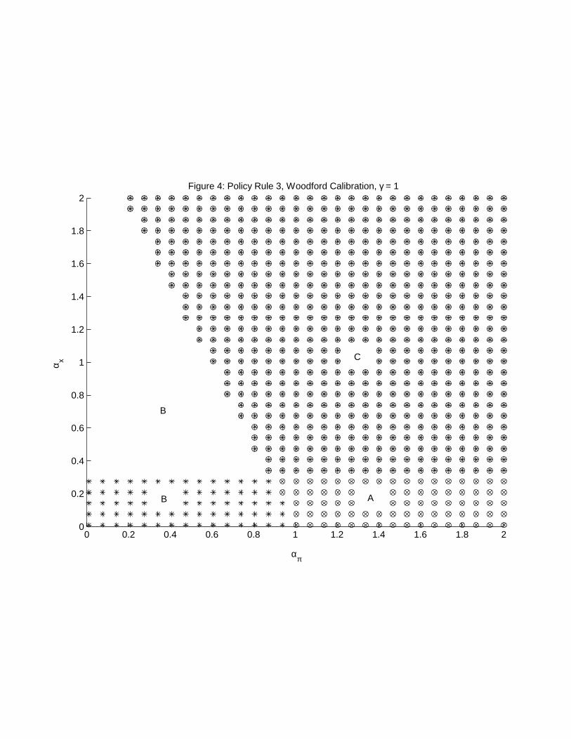
0 0.2 0.4 0.6 0.8 1 1.2 1.4 1.6 1.8 20

0.2

0.4

0.6

0.8

1

1.2

1.4

1.6

1.8

2Figure 4: Policy Rule 3, Woodford Calibration, γ = 1

απ

α x

B

C

B

A

0 0.2 0.4 0.6 0.8 1 1.2 1.4 1.6 1.8 20

0.2

0.4

0.6

0.8

1

1.2

1.4

1.6

1.8

2Figure 5: Policy Rule 3, Woodford Calibration, γ=1/2, β=1

απ

α x

1 1.2 1.4 1.6 1.8 20

0.05

0.1

0.15

0.2

0.25

0.3

0.35

0.4Figure 6: Policy Rule 3, λ=1, φ=1/.157, γ=1

απ

α x

0 1 2 3 4 5 6 7 8 9 100

1

2

3

4

5

6

7

8

9

10Figure 8: Policy Rule 4, φ=1/.157, λ=1, θ =.1, γ=1

απ

α x

B

A

C

0 1 2 3 4 5 6 7 8 9 100

1

2

3

4

5

6

7

8

9

10Figure 9: Policy Rule 4', φ = 6.3694, λ = 1, θ = 2, γ = 1

χπ

χ x