Monetary Policy in Financial Economies

By

Andrew Lee Smith

Submitted to the Department of Economics and the

Graduate Faculty of the University of Kansas

in partial fulfillment of the requirements for the degree of

Doctor of Philosophy

Committee members

Professor John W. Keating,

Chairperson

Professor William A. Barnett

Professor Robert DeYoung

Professor Ted Juhl

Professor Shu Wu

Date defended: May 29, 2014

The Dissertation Committee for Andrew Lee Smith certifies

that this is the approved version of the following dissertation :

Monetary Policy in Financial Economies

Professor John W. Keating, Chairperson

Date approved: May 29, 2014

ii

Abstract

This dissertation explores a critical question that arose naturally as a consequence

of the Great Recession: What is the appropriate role for and design of monetary

policy in financial economies? In addition to analyzing the unprecedented actions

taken by policy makers in the wake of the worst Financial Crisis since the Great

Depression, I also examine how conventional monetary policy instruments should

be designed and implemented in New-Keynesian economies - the workhorse model

of monetary policy for central banks.

Conventional Monetary Policy in Financial Economies

Unconventional monetary policy is designed as a response to financial crises.

However, in chapters 1, 2 and 3 I show that even conventional monetary pol-

icy must be adapted in financial economies. Specifically, I analyze the perfor-

mance of both Friedman ‘K-percent’ money growth rules and Taylor rules in

New-Keynesian models – the workhorse central bank model for monetary pol-

icy. However, unlike standard New-Keynesian models, I examine the theoretical

aspects of monetary policy in models with a meaningful financial sector. The

cumulative results of this section show the case against using monetary aggre-

gates by central bankers is significantly diminished once the financial sector is

included.

Chapter 1: Price vs. Financial Stability: A role for Money in Taylor

rules A consensus among central bankers, especially in the U.S., is that money

plays no meaningful role in the formation, nor execution of, monetary policy.

iii

This point is theoretically supported by New-Keynesian models in which optimal

policy can be described without any reference to money. However in Price vs.

Financial Stability: A role for Money in Taylor rules, my co-author and I turn

this logic on its head. By modeling a financial sector in an otherwise standard

New-Keynesian model, we show that augmenting a Taylor rule with a response

to the growth rate of money helps to offset the detrimental impacts of financial

sector disruptions.

Chapter 2: Determinacy and Indeterminacy in Monetary Policy Rules

with Money In Determinacy and Indeterminacy in Monetary Policy Rules with

Money, my co-author and I show the most basic of monetary policy rules, Milton

Friedman’s ‘k-percent’ rule fails to deliver a unique equilibrium, and therefore

creates economic instability. This result is in sharp contrast to the determinacy

properties of this rule in economies without a financial sector which feature no

bank produced assets. We then show the determinacy properties of this classic

monetary policy rule are restored when a Divisia monetary aggregate as formu-

lated by Barnett (1980) is used to measure the aggregate quantity of financial

and non-financial assets.

Chapter 3: A Working Solution to Working Capital Indeterminacy

Working capital refers to the financing firms’ require to fund inputs before they

receive payments for their output. When this channel is active, changes in inter-

est rates transmit through the usual demand/Euler channel and also a supply/-

marginal cost channel. The former dampens demand-pull inflation while the lat-

ter will exacerbate cost-push inflation. From a monetary policy standpoint, these

dual channels imply both a respective lower and an upper bound on the Monetary

Authority’s inflation response needed to guarantee the existence of a unique ratio-

nal expectations equilibrium (determinacy). In A Working Solution to Working

Capital Indeterminacy, I analytically show that Friedman’s ‘K-Percent’ rule is

iv

determinate in the presence of working capital channels. I additionally provide a

simple sufficient condition for the determinacy of interest rate rules reacting to

the nominal growth rate of the monetary aggregate: reacting greater than one

for one to changes in the growth rate of money guarantees determinacy. All of

these results are presented in the framework of a micro-founded New-Keynesian

model.

Unconventional Monetary Policy in Financial Economies

In chapters 4 and 5 of this dissertation, I turn the focus to unconventional mone-

tary policy. I use the term unconventional monetary policy to refer to the actions

taken by the U.S. Treasury and the Federal Reserve in the wake of the 2008 Fi-

nancial Crisis. In particular, the TARP legislation resulted in equity injections

into the largest U.S. commercial banks. Moreover, the Federal Reserve began

large scale asset purchases known as “Quantitative Easing” as a tool to improve

the functioning of credit markets. The Federal Reserve has especially focused on

purchasing Mortgage Backed Securities to: (i) improve the functioning of short-

term collateralized debt markets and (ii) increase home prices; with the goal that

both of these effects will improve the speed and strength of the recovery. The

results of this section provide insight into the transmission mechanism of these

policies and the role of housing, in both the recession and recovery.

Chapter 4: House Prices, Heterogeneous Banks and Unconventional

Monetary Policy Options In House Prices, Heterogeneous Banks and Un-

conventional Monetary Policy Options I answer salient questions in the wake of

the 2008 Financial Crisis. Why did a drop in home prices force big banks to

withdraw relatively more credit than smaller banks? What is the transmission

mechanism of equity injection into “Too Big to Fail” banks and “Quantitative

Easing” programs?

v

To answer these questions I develop a general equilibrium model with fully inte-

grated housing and financial markets. In addition to introducing housing-secured

debt into the financial market, the financial sector features heterogeneous banks

whereby “Too Big to Fail” institutions emerge in equilibrium. Unlike other mod-

els which rely on“Financial Shocks” and quadratic investment adjustment costs

to simulate a crisis episode, I take the alternative viewpoint that housing, and

housing secured debt, played a critical role in initiating and propagating the

crisis. By eschewing these typical assumption, including that all banks are the

same, I am able to show how a drop in housing demand can set off a financial

fire-sale effect.

Quantitatively, the model matches empirical correlations that the traditional

(Bernanke, Gertler, and Gilchrist, 1999) financial accelerator mechanism fails

to capture, including the correlation of finance premiums with home prices, in-

vestment and output. I then test the model’s qualitative predictions against an

estimated VAR. The results of these empirical comparisons support the model’s

financial structure. The model provides a framework to examine the ability of

QE policies and equity injections into big banks to mitigate a housing generated

recession. Although both are effective, the nuances of the policies are important.

A prolonged asset purchase program is preferable to a short-term equity injec-

tion; however, the model suggests the equity injections may have been necessary

to prevent an economic collapse at the acute stage of the 2008 Financial Crisis.

Chapter 5: The Foreclosure Accelerator versus the Financial Acceler-

ator: Housing and Borrower’s Net Worth The seminal work of Bernanke,

Gertler, and Gilchrist (1999) highlights how changes in the net worth of bor-

rowers can turn a typical downturn into deep protracted recession. However,

this celebrated financial accelerator model is silent with regards to the con-

nection between real-estate prices and borrower’s net worth. In this paper, I

vi

propose an alternative debt-contract in which agent’s net worth is largely in the

form of real-estate. This financial structure generates amplification and propaga-

tion of macroeconomic disturbances through a foreclosure channel as opposed to

investment-adjustment costs as in BGG. Contrary to the findings of Christiano,

Motto and Rostagno (2013), I estimate the equilibrium model using Bayesian

techniques and find that housing demand shocks, not risk shocks, drive finance

premiums. Finally, I answer some timely questions in the wake of the great reces-

sion including: Did the Federal Reserve’s low interest rate policy fuel the housing

bubble? How contractionary is the zero lower bound?

vii

Acknowledgements

I gratefully acknowledge fellowship support from the University of Kansas Grad-

uate College and additional funding and resources from the Department of Eco-

nomics. I would also like to thank: John Keating, my dissertation advisor and

coauthor of chapters 1 and 2; William Barnett and the Center for Financial Sta-

bility for access to high-quality monetary data which was used extensively in

chapters 1, 2 and 3; Robert DeYoung for directing me to the bank holding com-

pany data available from the FR Y-9C forms; Ted Juhl and Shu Wu for helpful

conversations and suggestions.

viii

Contents

1 Price versus Financial Stability: A role for Money in Taylor rules 1

1.1 Introduction . . . . . . . . . . . . . . . . . . . . . . . . . . . . . . . . . . . . 1

1.2 Model . . . . . . . . . . . . . . . . . . . . . . . . . . . . . . . . . . . . . . . 6

1.3 Calibration and Solution Strategy . . . . . . . . . . . . . . . . . . . . . . . . 19

1.4 Welfare Evaluation of Monetary Policy Rules . . . . . . . . . . . . . . . . . . 22

1.5 Comparative Statics, Robustly Optimal Policy and Determinacy . . . . . . . 31

1.6 Conclusion . . . . . . . . . . . . . . . . . . . . . . . . . . . . . . . . . . . . . 39

1.A Appendix: The Equilibrium System . . . . . . . . . . . . . . . . . . . . . . . 46

1.B Appendix: Tables . . . . . . . . . . . . . . . . . . . . . . . . . . . . . . . . . 65

2 Determinacy and Indeterminacy in Monetary Policy Rules with Money 67

2.1 Introduction . . . . . . . . . . . . . . . . . . . . . . . . . . . . . . . . . . . . 67

2.2 Model . . . . . . . . . . . . . . . . . . . . . . . . . . . . . . . . . . . . . . . 69

2.3 Friedman k-percent Rules . . . . . . . . . . . . . . . . . . . . . . . . . . . . 72

2.4 Interest Rate Rules with Money . . . . . . . . . . . . . . . . . . . . . . . . . 76

2.5 Numerical Analysis . . . . . . . . . . . . . . . . . . . . . . . . . . . . . . . . 79

2.6 Conclusion . . . . . . . . . . . . . . . . . . . . . . . . . . . . . . . . . . . . . 88

2.A Appendix: Proofs . . . . . . . . . . . . . . . . . . . . . . . . . . . . . . . . . 94

ix

3 A Working Solution to Working Capital Indeterminacy 103

3.1 Introduction . . . . . . . . . . . . . . . . . . . . . . . . . . . . . . . . . . . . 103

3.2 DSGE Model . . . . . . . . . . . . . . . . . . . . . . . . . . . . . . . . . . . 108

3.3 Working Capital Indeterminacy . . . . . . . . . . . . . . . . . . . . . . . . . 119

3.4 Adding Real Wage Rigidities . . . . . . . . . . . . . . . . . . . . . . . . . . . 127

3.5 Conclusion: A Working Solution to Working Capital Indeterminacy . . . . . 132

3.A Appendix: The Stationary, Non-Linear Model . . . . . . . . . . . . . . . . . 140

3.B Appendix: Proofs . . . . . . . . . . . . . . . . . . . . . . . . . . . . . . . . . 142

4 House Prices, Heterogeneous Banks and Unconventional Monetary Policy

Options 150

4.1 Introduction . . . . . . . . . . . . . . . . . . . . . . . . . . . . . . . . . . . . 150

4.2 A DSGE Model with Integrated Housing and Financial Markets . . . . . . . 153

4.3 VAR Tests of the Model’s Amplification Mechanism . . . . . . . . . . . . . . 178

4.4 Unconventional Monetary Policy . . . . . . . . . . . . . . . . . . . . . . . . . 193

4.5 Conclusion . . . . . . . . . . . . . . . . . . . . . . . . . . . . . . . . . . . . . 199

4.A Appendix: VAR Data and Complete Results . . . . . . . . . . . . . . . . . . 204

4.B Appendix: The Stationary, Non-Linear Model . . . . . . . . . . . . . . . . . 208

5 The Foreclosure Accelerator, Housing, and Borrower’s Net Worth 216

5.1 Introduction . . . . . . . . . . . . . . . . . . . . . . . . . . . . . . . . . . . . 216

5.2 A DSGE Model with Integrated Housing and Financial Markets . . . . . . . 218

5.3 Model Inference . . . . . . . . . . . . . . . . . . . . . . . . . . . . . . . . . . 236

5.4 Dissecting the Great Recession . . . . . . . . . . . . . . . . . . . . . . . . . 246

5.5 Conclusion . . . . . . . . . . . . . . . . . . . . . . . . . . . . . . . . . . . . . 259

5.A Appendix: The Stationary, Non-Linear Model . . . . . . . . . . . . . . . . . 264

x

List of Figures

1.1 Inside Money and Financial Distress . . . . . . . . . . . . . . . . . . . . . . 4

1.2 IRFs to a Negative Banking Productivity Shock . . . . . . . . . . . . . . . . 30

1.3 The Welfare Cost of Responding to Interest Rate Spreads . . . . . . . . . . . 32

1.4 Determinacy Region Under a Money Growth Targeting Rule . . . . . . . . . 37

1.5 Determinacy Region Under a Simple-Sum Growth Targeting Rule . . . . . . 62

2.1 Determinacy Region Under a Simple-Sum Growth Targeting Rule . . . . . . 81

2.2 Determinacy Region Under a Divisia Growth Targeting Rule . . . . . . . . . 85

2.3 Determinacy Regions Under Inertial Simple-Sum Growth Targeting Rules . . 86

2.4 Determinacy Regions Under Inertial Simple-Sum Growth Targeting Rules . . 87

3.1 The Taylor Principle . . . . . . . . . . . . . . . . . . . . . . . . . . . . . . . 105

3.2 Working Capital Indeterminacy . . . . . . . . . . . . . . . . . . . . . . . . . 107

3.3 IRFs to a Monetary Contraction with and without Sticky Wages . . . . . . . 129

3.4 Determinacy Region Under Inflation Targeting and Sticky Wages . . . . . . 130

3.5 Determinacy Region Under Inertial Inflation Targeting and Sticky Wages . . 131

3.6 Determinacy Region Under Money Growth Targeting and Sticky Wages . . . 133

3.7 Determinacy Region Under Inflation Targeting with a Money Growth Anchor

and Sticky Wages . . . . . . . . . . . . . . . . . . . . . . . . . . . . . . . . . 135

4.1 Real Home Prices and Asset Concentration in Big Banks . . . . . . . . . . . 153

xi

4.2 IRFs from the Equilibrium Model with and without Capital Constraints . . . 175

4.3 Illustrating the Asset Price Spiral from Big Bank Fire Sales . . . . . . . . . . 176

4.4 Model A: IRF to a Contractionary Aggregate Shock . . . . . . . . . . . . . . 185

4.5 Model A: IRF to a Decrease in the Large Bank Share . . . . . . . . . . . . . 186

4.6 Model A: IRF to an External Finance Premium Shock . . . . . . . . . . . . 187

4.7 Model A with Alternative Data: IRFs testing the Accelerator Mechanism . . 188

4.8 Model B: IRFs testing the Accelerator Mechanism . . . . . . . . . . . . . . . 189

4.9 Model B with Alternative Data: IRFs testing the Accelerator Mechanism . . 190

4.10 Model C: IRFs testing the Accelerator Mechanism . . . . . . . . . . . . . . . 191

4.11 Model C with Alternative Data: IRFs testing the Accelerator Mechanism . . 192

4.12 IRFs to a Large Housing Demand Shock and Various Unconventional Mone-

tary Policy Responses . . . . . . . . . . . . . . . . . . . . . . . . . . . . . . . 193

4.13 Indeterminacy and the Strength of the Asset-Price Spiral . . . . . . . . . . . 198

4.14 Model A: IRFs testing the DSGE Model’s Accelerator Mechanism . . . . . . 206

4.15 Model A: Historical Decompositions . . . . . . . . . . . . . . . . . . . . . . . 207

5.1 Housing, Finance Premiums and Real GDP . . . . . . . . . . . . . . . . . . 217

5.2 Illustrating Risk Shocks . . . . . . . . . . . . . . . . . . . . . . . . . . . . . 247

5.3 IRFs to a Contractionary Risk Shock . . . . . . . . . . . . . . . . . . . . . . 249

5.4 IRFs to a Contractionary Technology Shock . . . . . . . . . . . . . . . . . . 250

5.5 IRFs to a Contractionary Housing Demand Shock . . . . . . . . . . . . . . . 252

5.6 Historical Decompositions of Risk, Technology and Housing Demand Shocks 253

5.7 Historical Decompositions of the Financial Frictions Output Gap . . . . . . . 256

5.8 Historical Decompositions Testing the “too low for too long” Hypothesis . . 257

5.9 Historical Decompositions with and without the Zero Lower Bound . . . . . 259

xii

List of Tables

1.1 Welfare Results for Optimal Simple Rules . . . . . . . . . . . . . . . . . . . 24

1.2 Correlation of Real and Natural Interest Rates . . . . . . . . . . . . . . . . 25

1.3 Optimal Simple Rules with Additively Separable Preferences . . . . . . . . . 26

1.4 Optimal Simple Rules when the Efficient Output Gap is observable. . . . . . 27

1.5 Non-Optimized Rules . . . . . . . . . . . . . . . . . . . . . . . . . . . . . . 28

1.6 Correlation of Real and Natural Interest Rates . . . . . . . . . . . . . . . . 28

1.7 Inefficient Resource Costs . . . . . . . . . . . . . . . . . . . . . . . . . . . . 31

1.8 Elasticities of Optimal Policy Coefficients . . . . . . . . . . . . . . . . . . . . 33

1.9 Nash Equilibrium in Γ . . . . . . . . . . . . . . . . . . . . . . . . . . . . . . 35

1.10 Baseline Calibration of Parameters . . . . . . . . . . . . . . . . . . . . . . . 65

1.11 Equilibrium Variables and System of Equations . . . . . . . . . . . . . . . . 66

2.1 Determinacy Regimes Under a Simple-Sum Growth Targeting Rule . . . . . 80

2.2 Econometric Estimation of the Simple-Sum Error Term . . . . . . . . . . . . 82

2.3 Calibrated Parameters . . . . . . . . . . . . . . . . . . . . . . . . . . . . . . 83

2.4 Money Growth Rates During the Monetarist Experiment . . . . . . . . . . . 89

4.1 Cyclical Properties of the Model . . . . . . . . . . . . . . . . . . . . . . . . 174

4.2 Equity Injections vs. Quantitative Easing . . . . . . . . . . . . . . . . . . . 196

4.3 Bank Mergers and Acquisitions . . . . . . . . . . . . . . . . . . . . . . . . . 204

xiii

5.1 Model Calibrated Parameters . . . . . . . . . . . . . . . . . . . . . . . . . . 239

5.2 Model Parameters Priors and Posteriors - Economic Parameters . . . . . . . 242

5.3 Model Parameters Priors and Posteriors - Shocks . . . . . . . . . . . . . . . 245

5.4 FEVDs of Risk, Technology and Housing Demand Shocks . . . . . . . . . . . 254

xiv

Chapter 1

Price versus Financial Stability: A

role for Money in Taylor rules1

1.1 Introduction

The New-Keynesian sticky-price (NKSP) framework has become the workhorse model for

monetary policy evaluation due to its ability to provide a relevant role for monetary policy

while avoiding the well known Lucas critique. The research on optimal monetary policy in

these models has reached a clear consensus on two fronts. First, price stability is a paramount

policy concern while output should only be stabilized at its flexible price level. Second,

money is an inferior policy instrument due to persistent money demand shocks and offers

no information regarding the natural rates of output or interest. These conclusions, which

are robust across many model specifications, have led both academics and policy markers

towards “cashless models” of the economy and the monetary transmission mechanism. The

result, which is emphasized in Woodford (2003), is that optimal policy can typically be

described by an interest rate rule which reacts to the natural rate of interest, inflation and

the deviation of output from its flexible price (or natural) level . Curdia & Woodford (2009)

1This chapter is coauthored with John W. Keating, Department of Economics, The University of Kansas,Email: jkeating@ku.edu.

1

show this description of optimal policy extends even to a NKSP model with a financial sector

for the appropriately defined natural rate of interest.

However, in practice, policy makers know very little about the natural rate of output and

interest in real time. This has led researchers to consider optimal simple policy rules which

central banks could actually adopt. A rule is considered simple (Gali, 2008) if:

1. It makes the policy instrument a function of only observable variables

2. It does not require knowledge of the correct model

3. It does not require knowledge of model specific parameters

The desire to develop simple rules has led researchers to examine interest rate rules which

react to inflation and output growth, variables which are readily available at quarterly fre-

quencies, though sometimes with error. The optimality of such simple rules, usually with

no output growth response, has been verified in NKSP models under a wide array of model

specifications. Simply put, an interest rate rule responding to inflation appears to be the

best available simple rule (Schmitt-Grohe & Uribe, 2007).

Relatively less is known about optimal simple rules in models with financial sectors. To date

though, the literature on optimal simple rules in such models has often found no need to

deviate from inflation targeting interest rate rules. For example, in a model with financial

frictions, Faia & Monacelli (2007) find that responding to asset prices offers welfare gains

when the inflation coefficient is fixed at Taylor’s (1993) original values but these gains are

eliminated when the inflation coefficient is increased.2 Similarly, Dellas et al. (2010) find

that reacting to inflation of non-financial products offers the optimal simple rule in a setting

where banks are subject to supply shocks. However, none of these models which feature

financial sectors have examined the usefulness of monetary aggregates in simple rules.

2Curdia & Woodford (2010) provide similar evidence that such models may call for augmenting thestandard Taylor rule (with output and inflation coefficients fixed at Taylor’s (1993) original values) with areaction to the interest rate spread, although fully optimized simple rules are not analyzed.

2

If money is to serve a useful role in such contexts it seems most likely to do so as an

informational variable regarding the natural rate of interest. The desire for “simple rules”

and the readily available data on monetary aggregates at high frequencies suggests that

this is a promising chance to expand the set of useful information to policy makers in real

time. However, under typical money demand specifications, money is determined by output,

inflation, a single interest rate and money demand shocks.

Two things are worth noting under such a specification. First, money provides no additional

information to policy makers regarding the natural rates of output and interest not already

contained in output, inflation and policy rate data. Second, such a specification is completely

at odds with reality for broader monetary aggregates - inside money - whose equilibrium is

determined by both money demand which depends on a vector of interest rate spreads

and money supply by financial institutions and the shocks which originate therein. Hence,

under more realistic descriptions, movements in broad monetary aggregates are driven by

movements in non-policy rates and financial firms ability and willingness to supply monetary

assets.

This point is apparent in the graph above which shows the growth rate of Divisia M4 along

with the Federal Funds (policy) rate and output growth during the recent financial crisis.

Typical money demand specifications described above would have a hard time explaining

why money growth slowed while the Fed was cutting interest rates. One possibility is that

weak output growth was suppressing the demand for money, however, this story falls apart

in in 2009 when output growth began rising but money growth weakened further. While

suggestive, this graph provides some intuition into the behavior of inside money when the

economy is subjected to financial market disturbances, thus motivating the question of what

(if any) information can policy makers glean from broad monetary aggregates? In particular

we ask, is there an exploitable relationship between broad money growth and non-observable

variables such as the natural rate of interest when the economy is subject to financial shocks?

3

Q1−2006 Q1−2007 Q1−2008 Q1−2009 Q1−2010

−3

−2

−1

0

1

2

3

4

5

6

Inside Money and Financial Distress

Fed Funds

GDP Growth

Divisia M4 Growth

Figure 1.1: The shaded area marks the NBER recession dates. GDP and Divisia M4 growthrates are quarterly percentages while the Fed Funds rate is in annualized percentage points.

1.1.1 Related Literature

We are not the first to explore the usefulness of money in Taylor rules. Berger & Weber

(2012) explore the relationship between a variable they define as the money gap (the dif-

ference between the equilibrium quantity of money and estimated money demand) and the

natural interest rate in a prototypical NKSP model. They find that with noisy output gap

information the optimal money gap response is positive. Our work differs from theirs in at

least three regards. First, we search for simple rules which as defined above avoid the need

4

to use model specific variables nor estimate any model parameters. This point is especially

important since we explore the usefulness of monetary aggregates in Taylor rules for which we

employ the use of parameter- and estimation- free aggregation methods. Second, we examine

optimal monetary policy around a largely distorted steady state which requires a second order

accurate approximation to the model’s equilibrium condition as in Schmitt-Grohe & Uribe

(2004). Finally, we perform a complete analysis including numerically examining determi-

nacy regions for Taylor rules which react to Divisia monetary aggregate growth rates and

finding a robustly optimal policy rule under parametric uncertainty as in Giannoni (2002).

A second related paper is by Andres et al. (2009) who explore the empirical linkages between

dynamic money demand and the natural rate of interest. They find an empirical relation-

ship and suggest the possibility of exploiting this relationship in optimal monetary policy,

although they leave this for future work.

McCallum & Nelson (2011) also examine the link between monetary aggregates and the

natural rate of interest. They argue that the information in monetary aggregates could be

used to draw inference on the natural rate of interest provided the demand for the monetary

aggregate depends on a vector of interest rates. For example, assuming aggregate demand

depends on these real yields, then movements in these rates will affect the real policy rate

consistent with stable prices - the natural rate of interest. As they describe, movements in

these nominal yields will reflect movements in real yields aside from the policy rate causing

the quantity of money to co-move with the natural rate of interest. This is exactly the

path we pursue in this work. We spell out this relationship more carefully and provide an

implementable simple interest rate rule which could be put to use by central banks without

knowledge of model specific variables nor structural parameters.

1.1.2 Outline

The rest of this paper will proceed as follows. Next, we present the New-Keynesian model

developed by Belongia & Ireland (2013) to include a role for monetary aggregates and finan-

cial firms. Then we define the natural rates of interest and output in the model and show

5

that the financial market disturbances in the model decreases the natural rate of interest

which call for countercyclical monetary policy. We then examine the performance of opti-

mal “simple” interest rate rules using a micro-founded welfare metric and a second order

approximation to the model’s equilibrium conditions. With realistic assumptions regarding

the monetary authority’s information set we show that reacting to inflation alone, which is

typically optimal, fails to respond counter-cyclically to financial market disturbances leading

to poor welfare performance.

Instead optimal policy chooses to also react to the growth rate of Divisia monetary aggregates

which provide parameter- and estimation- free approximations to the true aggregate. We

show that policy rules with a positive Divisia growth response have well-behaved determinacy

properties satisfying a novel Taylor principle for monetary aggregates. Moreover, such rules

bring about a real policy rate which is highly correlated with the natural rate and maximizes

welfare. Interestingly, spread-adjusted Taylor rules are also highly correlated with the natural

rate but perform poorly from a welfare standpoint. We offer some insight into this counter-

intuitive result by showing that reacting to the interest rate spread fails to provide sufficient

liquidity following an adverse financial shock and ultimately induces unwanted volatility in

inflation . Finally, we end the paper with a robust policy prescription using a minimax

approach, as in Giannoni (2002), given the parameters driving financial and other stochastic

shocks remain uncertain.

1.2 Model

The model used in this analysis was developed by Belongia & Ireland (2013). It’s a stan-

dard sticky-price New-Keynesian model with the addition of a financial sector comprised of

perfectly competitive financial firms. The banks produce interest bearing deposits and loans

which requires a varying amount of real resources according to a stochastic process. As is

typical in these models, production of the final good requires inputs from intermediate goods

producers who have market power and hence can set their price given demand. The presence

6

of quadratic adjustment costs makes prices sticky which in turn makes monetary policy rel-

evant. Finally, the representative household works for, and holds stock in, the intermediate

goods firms. The household also demands loans and deposits from the financial firms which

depend on the vector of interest rates the household faces.

1.2.1 The Representative Household

The representative household enters any period t= 0,1,2, ... with a portfolio consisting of 3

assets. The household holds maturing bonds Bt−1, shares of monopolistically competitive

firm i ∈ [0,1] st−1(i), and currency totaling Mt−1. The timing of transactions requires the

household to carefully manage its portfolio of these assets. Central to this is the household’s

interaction with the representative bank with whom it makes deposits and takes loans.

The reason the household deposits and borrows money from the bank at the same time is

motivated in part by the description of the typical period t household budget constraints as

described by Belongia & Ireland (2013). This budgeting can be described by dividing period

t into 2 separate periods: first a securities trading session and then a transactions session.

1.2.1.1 Securities Trading Session

In the first part of period t the household purchases new securities which consists of bonds

Bt which pay one nominal unit of currency in period t for price 1/rt, where rt is the gross

nominal rate of interest, and shares of monopolistically competitive firm i, st(i) for a price

of Qt(i) per share. In this first portion of period t the household also acquires the liquidity

needed for the transactions period by securing loans from the representative bank totaling

Lt. The household ends this securities trading session by allocating its loans and the currency

remaining after trading securities between deposits and currency. Since deposits pay interest

they dominate currency in return, however the household will hold currency in equilibrium

due to the increased liquidity currency offers. The timing of these transactions is summarized

7

in the securities trading session budget constraint in (1) below.

Dt+Nt =Mt−1 +Bt−1 −1ˆ

0

Qt(i)(st(i)− st−1(i))di−Bt/rt+Lt (1.1)

1.2.1.2 Transactions Session

In the second portion of period t the household’s deposits mature yielding rDt Dt units of

currency which are then added to the currency the household set aside at the end of the

securities trading session - Nt. The household adds to this currency by supplying ht total

hours of labor to intermediate goods producing firm for a nominal wage rate PtWt. At the

same time each intermediate goods producing firm i ∈ [0,1] makes a dividend payment of

Ft(i) for each share owned by the household. The household must also pay back to the bank

all loans with interest totaling rLt Lt. The household then optimally allocates the remaining

currency between consumption goods PtCt and currency to be carried into next period Mt.

These activities are summarized in the transactions session budget constraint in (2) below.

Mt =Nt−PtCt+Wtht+

1ˆ

0

Ft(i)st(i)di+ rDt Dt− rLt Lt. (1.2)

1.2.1.3 Household Preferences

The true monetary aggregate which enters the household’s reduced from utility function is

given by the CES aggregator

MAt =

[

ν1ω (Nt)

ω−1ω +(1−ν)

1ω (Dt)

ω−1ω

] ωω−1

(1.3)

where ν calibrates the relative expenditure shares on currency and deposits and ω calibrates

the elasticity of substitution between the two monetary assets. In general, we need only

assume that the monetary aggregate is block-wise weakly separable within the household’s

utility function. The approach taken by Belongia & Ireland (2013) it to specify a shopping

8

time friction of the form

hst =1

χ

(

υtPtCt

MAt

)χ

(1.4)

where υt is a shock to the demand for monetary services following a first order autoregressive

process (in logs)

ln(υt) = (1−ρυ)ln(υ)+ρυln(υt−1)+ ευtwhere ευt ∼ i.i.d. (0,σ2

υ). (1.5)

We take this as our baseline calibration however the non additive-separability of the mone-

tary aggregate implies a real balance affect which has been challenged empirically (See for

example Ireland (2004a)). To show that our results do not hinge on this feature of the

household’s preferences we also consider the possibility that the monetary aggregate enters

the household’s utility function in an additively-separable form so that the term

ηmυtln

(

MAt

Pt

)

is added to the household’s utility function over consumption and leisure. In either case we

can define the household’s preferences recursively by

U = E0

∞∑

t=0

βtat [ln(Ct)−η(ht+hst )]

or

U = E0

∞∑

t=0

βtat

[

ln(Ct)−ηht+ηmυtln

(

MAt

Pt

)]

where at is a preference shock which follows a first order auto-regressive process (in logs)

ln(at) = ρaln(at−1)+ εatwhere εat ∼ i.i.d. (0,σ2

a). (1.6)

The representative household faces the problem of maximizing its lifetime utility subject to

its budget constraints. The household’s optimization problem and the resulting first order

9

necessary conditions are given in the appendix using Bellman’s equation.

1.2.2 The Representative Financial Firm

The representative bank creates demand deposits and originates loans for the representative

household in a purely competitive market. Specifically, in period t = 0,1,2, ... , the repre-

sentative bank creates interest bearing deposits in the amount Dt and originates loans in

the amount Lt. The pure-competition assumption implies the representative bank takes as

given the gross nominal interest rate it pays on deposits rDt and the gross nominal interest

rate it charges on loans rLt . The bank not only pays interest on deposits but also bears a

time-varying real cost ct(DtPt

) in order to create and service deposits defined by

ct(Dt

Pt) = xt

Dt

Pt.

The xt term is what makes the cost of producing deposits time varying, and in this case

stochastic, as this deposit cost function evolves according to the first order auto-regressive

process (in logs)

ln(xt) = (1−ρx)ln(x)+ρxln(xt−1)+ εxtwhere εxt ∼ i.i.d. N(0,σ2

x). (1.7)

The representative bank is also subject to the balance sheet constraint defined by the identity,

Lt = (1− τt)Dt (1.8)

where τt represents reserves held by the bank. In this model, the banks demand for reserves

varies stochastically according the first order auto-regressive process (in logs)

ln(τt) = (1−ρτ )ln(τ)+ρτ ln(τt−1)+ ετtwhere ετt ∼ i.i.d. N(0,σ2

τ ). (1.9)

10

Taking xt and τt as given, the profit maximization problem facing the representative bank

is defined by

maxDt,Lt

ΠBt = (rLt −1)Lt− (rDt −1)Dt−Ptxt

Dt

Ptsubjectto(1.8)

Substituting (1.8) into the objective function is a simple way to express the bank’s problem

and leads to the first order necessary condition for profit maximization

rDt = 1+(rLt −1)(1− τt)−xt. (1.10)

or

St = 1+(rLt − rDt ) = 1+ rLt (1− τt)+xt (1.11)

Equation (1.11) shows that the (gross) spread between deposits and loans varies endogenously

according to the market determined loan rate and varies exogenously according to the banks

demand for reserves and the marginal cost of producing deposits. The exogenous process for

reserves demand simulates times of financial distress when banks choose to decrease lending

activity and hoard deposits. The deposit cost shock acts to simulate negative banking

productivity shocks effectively raising the bank’s marginal cost of producing deposits. Just

as in Curdia & Woodford (2009), the existence of a time-varying loan-deposit spread has

implications for the natural rate of interest3 and ultimately optimal monetary policy.

1.2.3 The Representative Final Goods Producing Firm

The representative final goods producing firm maximizes period t profits for t = 0,1,2, ...

using a constant returns CES technology defined by

Yt =

1ˆ

0

Yt(i)θ−1

θ di

θθ−1

(1.12)

3See for example within their paper the natural rate of interest under financial frictions denoted rn,F Ft .

11

where Yt(i) is an input from intermediate goods producing firm i′s output. As is standard, we

assume the final goods market is purely competitive leaving the representative final goods

producing firm with no market power. Hence, behaving purely as a price taker in both

the output market Pt and the input markets Pt(i)∀ i ∈ [0,1] the representative final goods

producing firm solves

maxYt,Yt(i)i∈[0,1]

ΠFt = PtYt−

1ˆ

0

Pt(i)Yt(i)di (1.13)

subject to (1.12). This constrained maximization problem can easily be transformed into an

unconstrained problem by substituting the constraint into the objective function to eliminate

the choice variable Yt. The resulting first order necessary condition defines the factor demand

for each input Yt(i) as

Yt(i) =

[

Pt(i)

Pt

]−θ

Yt (1.14)

∀ i ∈ [0,1].

1.2.4 The Representative Intermediate Goods Producing Firm

Unlike the final goods market the intermediate goods market is not purely competitive. In-

stead each intermediate goods producing firm i ∈ [0,1] produces a differentiated product

leading to some degree of market power. To permit aggregation and allow for the consid-

eration of a representative intermediate goods producing firm i, we assume all such firms

have the same constant returns to scale technology which implies linearity in the single input

labor ht(i),

Yt(i) = Ztht(i). (1.15)

In each period t= 0,1,2, ... the representative intermediate goods producing firm rents ht(i)

units of labor from the representative household for a nominal market determined wage rate,

12

PtWt. The Zt term in (1.15) is an aggregate technology shock that follows a random walk

with drift (in logs)

ln(Zt) = ln(Z)+ ln(Zt−1)+ εztwhere εzt ∼ i.i.d. (0,σ2

z). (1.16)

The market power of each intermediate goods producing firm i leads to the ability for each

firm to set the price Pt(i) of its output Yt(i) each period t. The price setting ability of

each firm is constrained in two ways. First, each intermediate goods producing firm faces a

demand for its product from the representative final goods producing firm defined in (1.14).

Second, each intermediate goods producing firm faces a convex cost of price adjustment

proportional one nominal unit of the final good defined by Rotemberg (1982) to take the

form

Φ(Pt(i),Pt−1(i),Pt,Yt) =φ

2

[

Pt(i)

Pt−1(i)π−1

]2

YtPt. (1.17)

Every intermediate goods producing firm i ∈ [0,1] maximizes its period t real price per

share denoted by Qt(i)Pt

. Though the firm maximizes period t share price, the costly price

adjustment constraint makes the intermediate goods producing firm’s problem dynamic (and

recursive) as shown in the appendix. Mathematically summarizing, each intermediate goods

producing firm solves to following dynamic problem,

maxht(i),Pt(i)∞

t=0

Qt(i)

Pt

subject to the constraints (1.14), (1.15) and (1.17). In a symmetric equilibrium the log-

linearized first order condition of the above problem takes the form of a New-Keynesian

Phillips Curve (NKPC) relating current inflation to the average real marginal cost and

expected future inflation. The resulting NKPC can be calibrated to match the NKPC

13

derived from Calvo style price adjustment based on the frequency of price changes4.

1.2.5 The Central Bank

We close the model by specifying the general class of monetary policy rules we consider by

rt = ρrrt−1 +φππt+φy(Yt− Yt−1)+φmµDivisiat −φsSt (1.18)

in log-deviations from steady state5 with ρr in [0,1] and φπ, φy, φm and φs in [0,∞) and

S = rLt − rDt . The policy rule is restricted to be both linear in logs and react only to

observable model non-specific variables. The second restriction is key for the policy rule

to be implementable as stressed in Schmitt-Grohe & Uribe (2007) and Faia & Monacelli

(2007). For this reason we include the growth rate of output instead of deviations of output

from its natural level.6 Orphanides (2003) stresses the latter is not available to policy

makers in real time without significant measurement error. For robustness, we also examine

the case when the efficient level of output is available to policy makers in real time (See

section 4.2.3). The implementability restriction also requires that we provide a measure of

the monetary aggregate that doesn’t require knowledge of its functional form nor the values

of its parameters. We discuss this issue below.

1.2.5.1 The Monetary Aggregation Problem

The general problem of tracking an unknown aggregator function without estimation is not

new. The solution lies in statistical index number theory as advanced by Diewert (1976)

and specifically applied to monetary aggregation by Barnett (1978, 1980). The focus of

this field is to provide parameter- and estimation-free aggregates. One such index number

performs this task with a known level of accuracy. The Divisia monetary aggregate provides

4However, the two pricing assumptions will in general result in different NKPCs up to a second orderapproximation. This difference will generally lead to different welfare-loss functions when approximatedaround a distorted steady-state as shown in Lombardo & Vestin (2008).

5To be clear, for any variable Xt, Xt = ln(Xt)− ln(X).6This natural level of output is defined in section 3 below.

14

a second-order accurate approximation to the growth rate of MAt .7 We now define the Divisia

monetary aggregate in this model.

Definition 1.1. The growth rate of the Divisia monetary aggregate is defined by

ln(µDivisiat ) =

(

sNt + sNt−1

2

)

ln

(

NtNt−1

)

+

(

sDt + sDt−1

2

)

ln

(

Dt

Dt−1

)

(1.19)

where sNt and sDt are the expenditure shares of currency and interest bearing deposits re-

spectively defined by

sNt =uNt Nt

uNt Nt+uDt Dt=

(rLt −1)Nt(rLt −1)Nt+(rLt − rDt )Dt

(1.20)

and

sDt =uDt Dt

uNt Nt+uDt Dt=

(rLt − rDt )Dt

(rLt −1)Nt+(rLt − rDt )Dt. (1.21)

Since the definition of the Divisia monetary aggregate only requires knowledge of current

and one period lagged monetary component quantities and interest rates our policy rule

specified in (1.18) is a simple rule which could actually be implemented by central banks

facing limited real time information. For example in the U.S., the St. Louis Fed’s MSI series

provides Divisia monetary aggregates for M1 and M2 at a monthly frequency8.

We embed the Divisia approximation to the true aggregate, as opposed to alternative simple-

sum approximations, in the policy rule due to the superiority of the Divisia monetary aggre-

gate in tracking the true aggregate - as shown in this model by Belongia & Ireland (2013).

7The ability to track any function which is homogeneous of degree one (as all sensible aggregator functionsare) to second order accuracy places the Divisia aggregate in Diewart’s (1976) class of superlative index

numbers.8Private organizations such as the Center for Financial Stability have recently begun providing broader

Divisia monetary aggregates at monthly frequencies as well.

15

9 For thoroughness we examine the performance of the more common simple-sum aggregate

ln(µSimple−Sum) = ln

(

Nt+Dt

Nt−1 +Dt−1

)

(1.22)

in place of the Divisia aggregate in the above policy rule. The rule results in indeterminacy

in most of the parameter space. In the appendix we show the determinacy region and show

through linearization the size of the error of the simple-sum aggregate in tracking the true

aggregate in this model.

1.2.6 Market Clearing

It is now possible to define the equilibrium conditions which close the model. Market clearing

in the labor market requires that labor supply equal labor demand, or

ht =

ˆ 1

0ht(i)di. (1.23)

Equilibrium in the final goods market requires that the accounting identity

Yt = Ct+xtDt

Pt+φ

2

[

Πt

Π−1

]2

Yt (1.24)

holds as well. Equilibrium in the money market, equity market and bond market requires

that at all times

Mt =Mt−1 (1.25)

st(i) = st−1(i) = 1 (1.26)

Bt =Bt−1 = 0 (1.27)

9For more general research examining the Divisia monetary aggregate’s properties relative to alternativesimple-sum measures see the following works. At paper length Barnett & Chauvet (2011b); Belongia (1996)and at book length Barnett & Singleton (1987); Belongia & Binner (2000); Barnett & Serletis (2000); Barnett& Chauvet (2011a); Barnett (2012).

16

respectively. Finally, imposing the symmetry among the intermediate goods producing firms

requires that in equilibrium

Yt(i) = Yt, Pt(i) = Pt, Ft(i) = Ft, and Qt(i) =Qt. (1.28)

1.2.7 Welfare Relevant Natural Rates of Output and Interest

Central to the analysis of optimal monetary policy in NKSP models are the concepts of

the natural rate of output and interest. These measures respectively represent the level

of output and the real interest rate in an identical economy as the one described without

the presence of sticky prices. Woodford (2003) has shown that these concepts play the key

role in optimal monetary policy, hence we provide the relevant definitions in this model to

show that financial market supply shocks affect these variables and hence impact optimal

monetary policy rules - similar to the model of Curdia & Woodford (2009). For cohesiveness,

we use Woodford’s (2003, pg. 302) definition of the natural rate of interest in a monetary

economy.

Definition 1.2. The natural rate of output is the equilibrium level of output at each point

in time that would prevail under flexible prices, given a monetary policy that maintains

a constant interest rate spread uAt = rLt − rAt between non-monetary (bonds or loans) and

monetary riskless short-term assets (currency and deposits).

The aggregate interest rate on monetary riskless short-term assets rAt in Definition 2 is the

nominal return for holding one unit of the monetary aggregate in period t. This interest rate

can be derived from first principles10 providing a coherent way to think about interest rates

in an economy with multiple monetary assets each with different rates of return. Therefore

the aggregate user-cost uAt = rLt − rAt provides a natural analogue to the the interest rate

spread between bonds and a single monetary asset, the environment considered in Woodford

(2003, Ch. 4). Applying this definition to the log-linearized equilibrium conditions results in

10We carefully define this in the appendix. See Eq. 1.A.18.

17

a natural rate of output that depends only on the model’s stochastic disturbances. As shown

in the appendix, the resulting expression for the natural rate of output (in log deviations

from steady state11) is given by

Y nt = Zt−Ψyυυt−Ψy

xxt−Ψyτ τt (1.29)

where Ψyx and Ψy

τ are positive in all reasonable calibrations 12. As is standard from the

real business cycle literature, positive technology shocks increase the productive capacity of

the economy under flexible prices. Novel here is the appearance of the financial shocks in

this expression. Adverse shocks to the financial intermediary’s cost of producing monetary

assets and willingness to supply loans will behave as negative technology shocks and lower

the natural rate of output.

However, there is a striking difference between financial and goods market supply shocks

from a policy standpoint. This difference lies in how these shocks affect the natural rate of

interest. The expression for the natural rate - given the above definition of the natural rate

of output - is shown below (in log deviations from steady state 13)

rnt = (1−ρa)at− (1−ρz)Zt−Ψrx(1−ρx)xt−Ψr

τ (1−ρτ )τt (1.30)

where Ψrx > 0 and Ψr

τ > 0 and independent of how money enters the utility function. The

implication for monetary policy is that responding to adverse financial supply shocks calls for

countercyclical policy, meanwhile responding to adverse technology shocks calls for procyclical

policy. The challenge facing the monetary authority is how to form a policy rule which is

optimal in this environment given the lack of information they have on the natural rate. We

show the monetary aggregate provides valuable information regarding movements in this key

11To be clear, for any variable Xt, Xt = ln(Xt)− ln(X).12The sign of Ψy

υ changes depending on the specification of preferences. For additively separable utility itis always positive however for non additively-separable utility it is negative.

13To be clear, for any variable Xt, Xt = ln(Xt)− ln(X).

18

variable.

1.3 Calibration and Solution Strategy

At this point it is useful to proceed by assigning numerical values to the model’s parameters.

Following the calibration strategy pioneered by Kydland & Prescott (1982) we assign values

to parameters in a fashion that allows us to match key features of U.S. data. Since the model

used here was developed by Belongia & Ireland (2013) we take many of the values used in

their study. Moreover, the model is similar in many regards to the ones estimated by Ireland

(2004a,b) providing reliable estimates of the parameters defining the stochastic processes.

Table 1.10 in the appendix summarizes the choice of parameter values. We end the section

with a brief discussion of the solution procedure.

1.3.1 Calibration

The model is calibrated to the U.S. economy so that one period represents one quarter. We

set β = .99 and we set Z = 1.005 which is consistent with annual real GDP growth of 2%.

These facts imply an annual real interest rate of 6% which is in line with the RBC calibration

literature (Kydland & Prescott, 1982). We set π = 1.005 which matches the official inflation

target of the Fed of 2% per year. The disutility of work parameter η = 2.5 so that one-third

of the household’s time is spent working. When money is non-separable setting χ= 2 makes

the shopping time specification quadratic. As for the CES monetary aggregator MAt , the

calibrations of ω = 1.5 specifies more substitutability between currency and deposits than

the Cobb-Douglas specification and setting ν = .225 pins down the ratio of steady state

ratio NN+D = .1, the U.S. average ratio of currency to simple-sum M2 since 1959. Similarly,

υ = .4 matches the steady state ratio N+DPC = 3.3, the average of simple-sum M2 to nominal

consumption expenditures over the same period.

On the production side of the economy we set the elasticity of substitution between in-

termediate goods θ = 6 yielding a steady state mark-up of 20% over marginal cost for the

monopolistic firm following Ireland’s estimates (2000; 2004a; 2004b). The setting for the

19

cost of price adjustment φ= 50 implies a NKPC that coincides with Calvo style pricing dy-

namics when the average duration of a price is slightly more than one year (Ireland, 2004b).

Regarding the production of financial assets and services setting τ = .02 sets the steady level

of reserves to 2%, the average ratio of St. Louis adjusted reserves to the simple-sum deposit

components of M2 since 1959 (Ireland, 2011). From the goods market clearing condition,

setting x= .01 implies in steady-state 3% of output is devoted to banking activities, slightly

less than the 3.6% derived from “Federal Reserve banks, credit intermediation, and related

activities” on average over the last decade according to the Bureau of Economic Analysis.

The fact that our model implies a lower average is accurate considering the limited scope

of the activities carried out by the financial sector in this model (Belongia & Ireland, 2006,

2013).14

Many of the stochastic processes driving the model have been estimated in Ireland (2004a).

Specifically, we use Ireland’s estimates of the persistence and standard error of the money

demand, preference and technology15 shocks. However, the parameters driving the financial

shocks have not yet been estimated in the literature. Dellas et al. (2010) calibrate a model

with reserves demand and bank cost shocks interpreting the calibrated values from a fre-

quentists perspective. Following their approach to calibrating the financial shocks standard

errors we set στ and σx so that an increase in banks demand for reserves and an increase

in the benchmark-M2 aggregate interest rate spread of the magnitude witnessed during the

recent financial crisis occurs once every 80 years on average in our model, assuming normal-

ity.16 The time period of 80 years acknowledges the time span between the Great Depression

14As previously mentioned, the deposit-cost shock also dictates the spread between the benchmark interestrate rL

t and the deposit rate rDt . To confirm the logic of the calibration note the annualized spread between

the benchmark rate and the aggregate rate rL −rA in the model’s steady-state is about 4.6%, which is veryclose to the average spread between the benchmark rate and the Divisia M2 aggregate interest rate in U.S.data running from January 1967 to September 2009 equal to 4.2% using data from the Center for FinancialStability. Hence, the ability of the model to emulate the data along this added dimension reconfirms thecalibration put forth by Belongia & Ireland (2013).

15The persistence parameter for the technology shock is set to 1 throughout the paper.16More specifically reserves measured using the ratio of St. Louis adjusted reserves to the deposit compo-

nents of M2 spiked from slightly over .02 in September 2008 to over .21 in June of 2011. Hence we set στ sothat P (τ > ln(.21)− ln(.02)) = 1/320 where τ ∼N(0,σ2

τ

∑11i=0 ρ

2iτ ). Similarly, the spread between the bench-

mark rate and the Divisia M2 aggregate rate stood at just 2.8% in July 2008 and in just one quarter the spread

20

and the recent financial crisis. This specification of στ is conditional on a value of ρτ . When

calibrating ρτ and ρx we once again follow Belongia & Ireland (2013) and set ρτ = .5 and

ρx = .5. However since these are only calibrated values and not estimates in section 5.2 we

perform a robust policy calculation allowing ρτ and ρx to vary between [0, .99]. Moreover,

in this section we relax the normality assumption used here to calibrate στ and σx to a

student’s t-distribution with significantly “fatter-tails” as called for by much of the finance

literature (Mandelbrot, 1963; Fama, 1965).

1.3.2 Solution Strategy

Solving the full non-linear model is not possible hence we resort to approximation techniques.

Two main difficulties are encountered. First, the model as presented does not exhibit a

deterministic steady-state due to the unit root in the technology process and the price

level. To deal with this we detrend most nominal variables by the price level and the

technology shock. Details of this detrending are handled in the appendix. Second, a first

order approximation is adequate for questions of local determinacy however for proper welfare

rankings we must use (at least) a second order approximation17 (Schmitt-Grohe & Uribe,

2004). Therefore we analyze determinacy using a linear approximation to the model around

the steady state implied by the competitive equilibrium and we evaluate welfare using a

second-order approximation around the Ramsey planner’s steady state with all distortions

in place as in Schmitt-Grohe & Uribe (2007).18We discuss this choice and provide more

details regarding the welfare evaluation in the section below.

spiked to 4.47%. In order to simulate such liquidity shocks we set σx so that P (x> ln(4.47)− ln(2.8)) = 1/320where x∼N(0,σ2

x). The value obtained for σx is very close the one obtained by Belongia & Ireland (2006)when they calibrate an RBC version of the model to match their estimated VAR standard errors.

17An exception to this fact is when the steady state distortions are small. This case is the focus ofWoodford (2003) and Curdia & Woodford (2010).

18It’s worth noting, the determinacy results also hold around the Ramsey planner’s steady state and thewelfare results are qualitatively identical if we approximate the model around the competitive equilibrium’ssteady state.

21

1.4 Welfare Evaluation of Monetary Policy Rules

We now present our main results of the paper. Most importantly, optimal monetary policy

features a positive response to the growth rate of the Divisia monetary aggregate. We show

that policy rules which respond to the growth rate of money result in real policy rates which

are highly correlated with the natural rate of interest. However, this condition appears to

be only necessary, not sufficient for good policy. Specifically, responding to the interest rate

spread increases the correlation between the real and natural rates of interest but fails to

deliver good policy. Instead, such rules increase the variance of inflation and the resources

allocated to financial intermediation - leading to detrimental welfare effects.

1.4.1 Welfare Evaluation Methodology

The focus of the current literature on optimal simple monetary policy rules has been to

use a micro-founded measure of welfare without imposing any upper bound on the size of

distortions generated in the competitive equilibrium. Following this line of work we use a

second order approximation to the household’s utility function as our metric for ranking

alternative policy rules. Moreover, the appropriate expectation of welfare is the conditional

as this measure takes into account welfare gains and losses accrued while transitioning from

the deterministic steady state to the stochastic steady state implied by the given policy rule

(Kim et al., 2005). This does however give meaning to the initial state at which policy

is evaluated. For this reason we evaluate all policies around the Ramsey planner’s steady

state. Hence, we generally have the following welfare metric, regardless of how preferences

over money are specified.

W0 = E0

∞∑

t=0

βt[

u(Ct,ht,MAt

Pt,at,υt)

]

(1.31)

We take a second order approximation to u(Ct,ht,MA

tPt,at,υt) around the Ramsey steady state

allowing for us to express welfare as the weighted sum of conditional means and covariances

22

of the arguments in the utility function. We then evaluate these conditional moments using

decision rules found from the second order approximation to the equilibrium conditions.19

We report our results as consumption equivalent shares. Specifically if W∗0 is the welfare

obtained under an optimal policy then Ω is the share of the generic consumption stream the

household would need to equate welfare under the sub-optimal policy to the optimal welfare

W∗0 = E0

∞∑

t=0

βt[

u(Ct(1+Ω),ht,MAt

Pt,at,υt)

]

. (1.32)

Given this definition, Ω is simply the welfare cost in consumption terms of sub-optimal

policies.

1.4.2 Optimal Simple Rules

We now turn our attention to optimal simple rules of the form

rt = ρrrt−1 +φππt+φy(Yt− Yt−1)+φmµDivisiat −φsSt

in log-deviations from steady state with ρr in [0,1] and φπ, φy, φm and φs in [0,∞) and

St = 1+(rLt −rDt ). The most significant departure from policy rules specified in the literature

on optimal simple rules is the inclusion of the (growth rate of the) Divisia monetary aggregate

and the spread between loans and deposits. We show below that optimal policy calls for a

response to the Divisia monetary aggregate but not the interest rate spread. In particular,

we highlight the increased correlation of the real interest rate with the natural rate of interest

when policy reacts to the Divisia aggregate. Moreover, reacting to Divisia achieves this high

correlation at a low inflation volatility compared to rules which react to the interest rate

spread. We also examine optimal policy under additively separable preferences over money

and under the assumption policy makers have knowledge to the efficient output gap and find

19To prevent the order of the forecast, and the forecast itself, from exploding we implement the pruningmethod proposed in Kim et al. (2005). More specifically, we use a first order approximation to the equilibriumconditions to evaluate the conditional variances and then use these conditional variances in the second orderapproximation to evaluate the means. See Kim et al. (2005) and specifically Section 7 therein.

23

our results to be robust.

1.4.2.1 Baseline Results

We first present our baseline results assuming policy makers only have knowledge of the

growth rate of output, current and past interest rates, inflation and the growth rate of the

monetary aggregate. The results of the central bank’s optimization are presented in Table

1.1.

Table 1.1: Welfare Results for Optimal Simple Rules

rt = ρrrt−1 +φππt+φy

(

Yt− Yt−1

)

+φmµDivisiat −φsSt

Optimal Policy Rule Coefficients Welfare Cost

Policy Rule ρ∗r φ∗

π φ∗y φ∗

m φ∗s Ω1

Optimal 0 3.234 0 2.366 0 0

Optimal φπ = 0 0 − 0 4.217 0 .0304

Optimal φm = 0 0 3.6780 0.8982 − 0 .1551

Optimal φm = φy = 0 0 4.070 − − 0 .1736

1 Ω is the % of consumption required to equate welfare under any given policy ruleto the one under the optimal policy (see Eq. (1.32)). Welfare is calculated asconditional to the initial deterministic Ramsey steady state.

Several points are worth noting. (i.) First, responding to the Divisia monetary aggregate

is essential to achieve optimal welfare. Notice the welfare cost of not responding to the

Divisia aggregate is nearly 5 times as large as the welfare cost of not responding to inflation.

One reason for the importance of responding to the Divisia monetary aggregate is due to

its ability to provide an indicator in movement of the natural rate. Section 2.7 shows the

natural rate of interest falls in response to financial shocks calling for expansionary policy.

Only focusing on inflation, or even output growth, fails to provide sufficient expansion. To

verify this, Table 1.2 presents the correlation between the natural rate (See Eq. (1.30)) and

real interest rate under optimal rules with and witohut money.

(ii.) Second, unlike in Schmitt-Grohe & Uribe (2007) and Faia & Monacelli (2007) - without

considering monetary aggregates (φm = 0) - responding to output growth is welfare enhanc-

ing. The reason for the difference lies in the stochastic rank of our economy versus theirs.

24

Table 1.2: Correlation of Real and Natural Interest Rates

Policy Rule Corr(rnt , rt−Etπt+1)

Optimal .8281

Optimal φπ = 0 .8355

Optimal φm = 0 .0377

Their economies are driven by aggregate demand and technology shocks, which affect the

natural and efficent levels of output symmetrically. In our economy on the other hand, the

presence of financial shocks - which affect the natural level of output but no the efficient

level - induces policy makers to deviate from strict inflation targeting. Our third point

(iii.) responding to the interest rate (loan-deposit) spread decreases welfare. We expand

on this counter-intuitive point below where we consider non-optimized rules, including a

spread-adjusted Taylor rule as advocated by Taylor (2008).

1.4.2.2 Results with Additively Separable Utility

One may wonder if we arrive at the above results due to the specification of non-additively-

separable preferences over money and consumption. As Ireland (2004a) highlights this as-

sumption results in money showing up directly in the IS equation and the NKPC. The

resulting real-balance effect may lead to a bias to stabilize the monetary aggregate. In this

section we directly address this concern. The results below verify that money should enter

the policy rule due to the information it conveys to policy makers regarding developments

in financial markets, not because of the specification of preferences over money.

Interestingly when money enters the policy rule, it ends up in the IS and NKPC as pointed

out by McCallum & Nelson (2011). Hence, Table 1.3 suggests money should enter these

equations from a normative standpoint, regardless of the empirical motivation for money

entering these equations (See e.g. (Ireland, 2004a)). Specifically, under additive separability

the optimal coefficients are qualitatively similar to the optimal coefficients under our baseline

specification. Qualitatively however, optimal policy continues to respond only to inflation

and Divisia. What’s more, under these preferences the welfare cost of not responding to

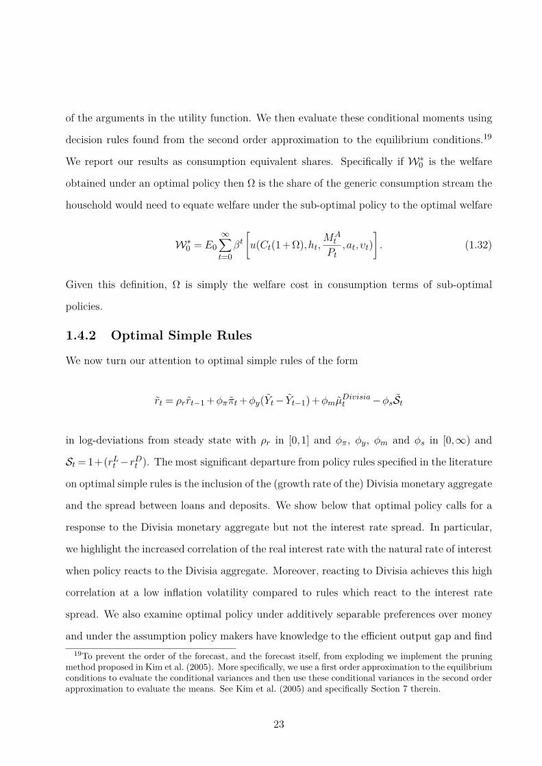
25

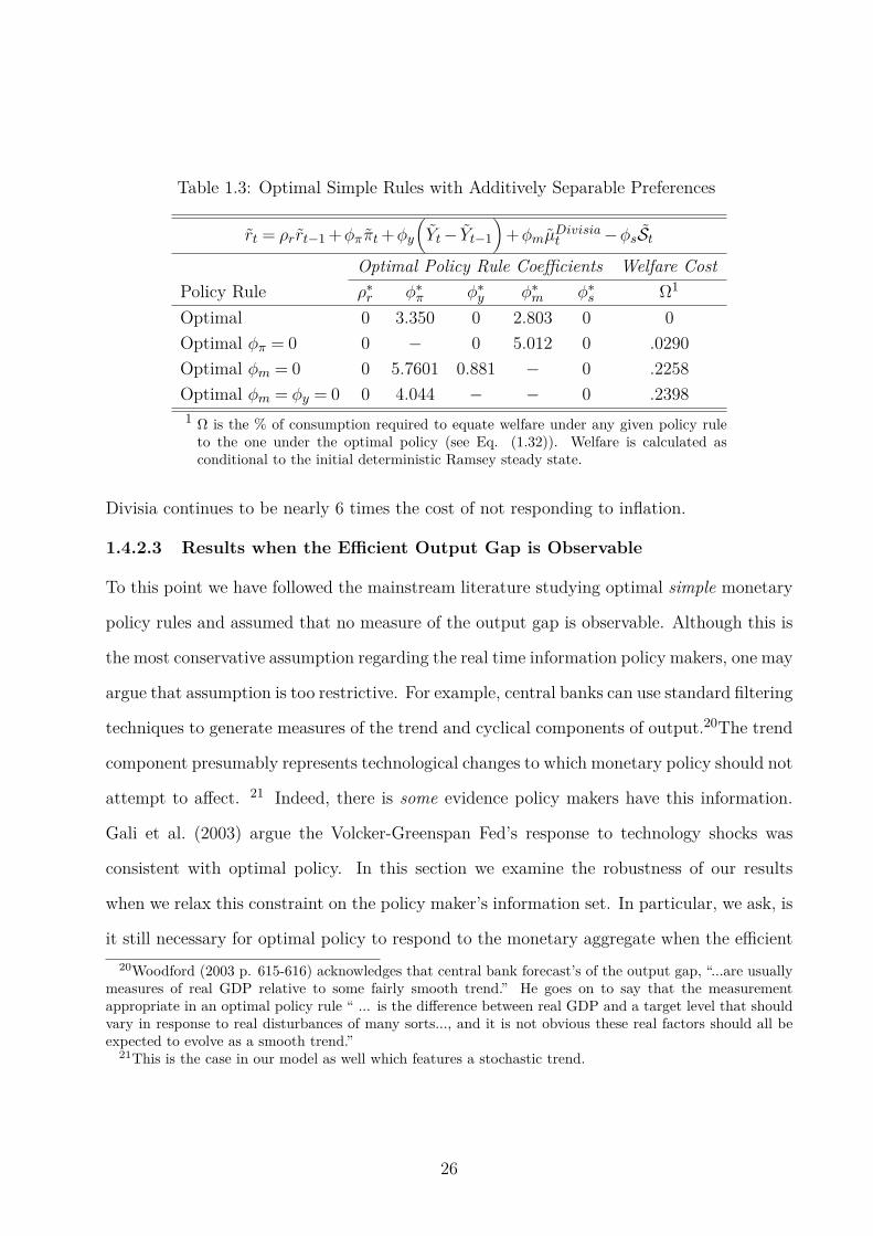
Table 1.3: Optimal Simple Rules with Additively Separable Preferences

rt = ρrrt−1 +φππt+φy

(

Yt− Yt−1

)

+φmµDivisiat −φsSt

Optimal Policy Rule Coefficients Welfare Cost

Policy Rule ρ∗r φ∗

π φ∗y φ∗

m φ∗s Ω1

Optimal 0 3.350 0 2.803 0 0

Optimal φπ = 0 0 − 0 5.012 0 .0290

Optimal φm = 0 0 5.7601 0.881 − 0 .2258

Optimal φm = φy = 0 0 4.044 − − 0 .2398

1 Ω is the % of consumption required to equate welfare under any given policy ruleto the one under the optimal policy (see Eq. (1.32)). Welfare is calculated asconditional to the initial deterministic Ramsey steady state.

Divisia continues to be nearly 6 times the cost of not responding to inflation.

1.4.2.3 Results when the Efficient Output Gap is Observable

To this point we have followed the mainstream literature studying optimal simple monetary

policy rules and assumed that no measure of the output gap is observable. Although this is

the most conservative assumption regarding the real time information policy makers, one may

argue that assumption is too restrictive. For example, central banks can use standard filtering

techniques to generate measures of the trend and cyclical components of output.20The trend

component presumably represents technological changes to which monetary policy should not

attempt to affect. 21 Indeed, there is some evidence policy makers have this information.

Gali et al. (2003) argue the Volcker-Greenspan Fed’s response to technology shocks was

consistent with optimal policy. In this section we examine the robustness of our results

when we relax this constraint on the policy maker’s information set. In particular, we ask, is

it still necessary for optimal policy to respond to the monetary aggregate when the efficient

20Woodford (2003 p. 615-616) acknowledges that central bank forecast’s of the output gap, “...are usuallymeasures of real GDP relative to some fairly smooth trend.” He goes on to say that the measurementappropriate in an optimal policy rule “ ... is the difference between real GDP and a target level that shouldvary in response to real disturbances of many sorts..., and it is not obvious these real factors should all beexpected to evolve as a smooth trend.”

21This is the case in our model as well which features a stochastic trend.

26

output gap22 is observable?

Table 1.4: Optimal Simple Rules when the Efficient Output Gap1 is observable.

rt = ρrrt−1 +φππt+φgGet +φmµ

Divisiat −φsSt

Optimal Policy Rule Coefficients

ρ∗r φ∗

π φ∗g φ∗

m φ∗s

Optimal 0 3.234 0 2.366 0

1 The Efficient Output Gap in levels is given byGe

t = YtY e

t= η Yt

Ztas shwon in the appendix (See Eq.

(1.A.32)).

The results in this section show two things. First, when the efficient output gap is observable

optimal policy still responds to the Divisia monetary aggregate. Second, and more to the

point, knowledge of the efficient output gap has no impact on the optimal policy coefficients

- the only variables in the policy rule with a non-zero coefficient are inflation and the growth

rate of the Divisia aggregate. This result stresses the importance of financial shocks shaping

the optimal simple policy rule. In particular, policy makers must now deal with inefficient

resource costs from financial intermediation in addition to inefficient resource cost stemming

from price adjustment and inefficient rents due to monopolist’s market power.

1.4.3 Non-Optimized Rules

It is insightful at this point to compare the performance of policy rules which have historically

provided a description of actual Fed policy with our optimal rules. In particular, we can

infer the welfare gains of switching from current policy to our prescribed optimal rule. We

examine the performance of the original Taylor rule (Taylor, 1993) and the forward-looking

rule estimated in Clarida et al. (2000) which provides a good description of Fed policy during

the Volcker-Greenspan era. Not surprisingly, the above rules lack an aggressive enough

response to the financial market shocks and hence lack the necessary correlation with the

natural rate of interest. Addressing this issue, Taylor (2008) recently suggested allowing the

22The level of the efficient output gap is given by Get = Yt

Y et

= η YtZt

, as shown in the appendix (See Eq.

(1.A.32)).

27

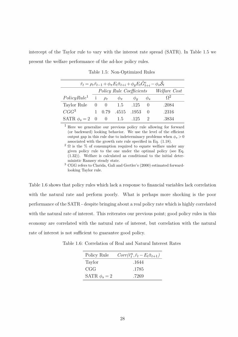
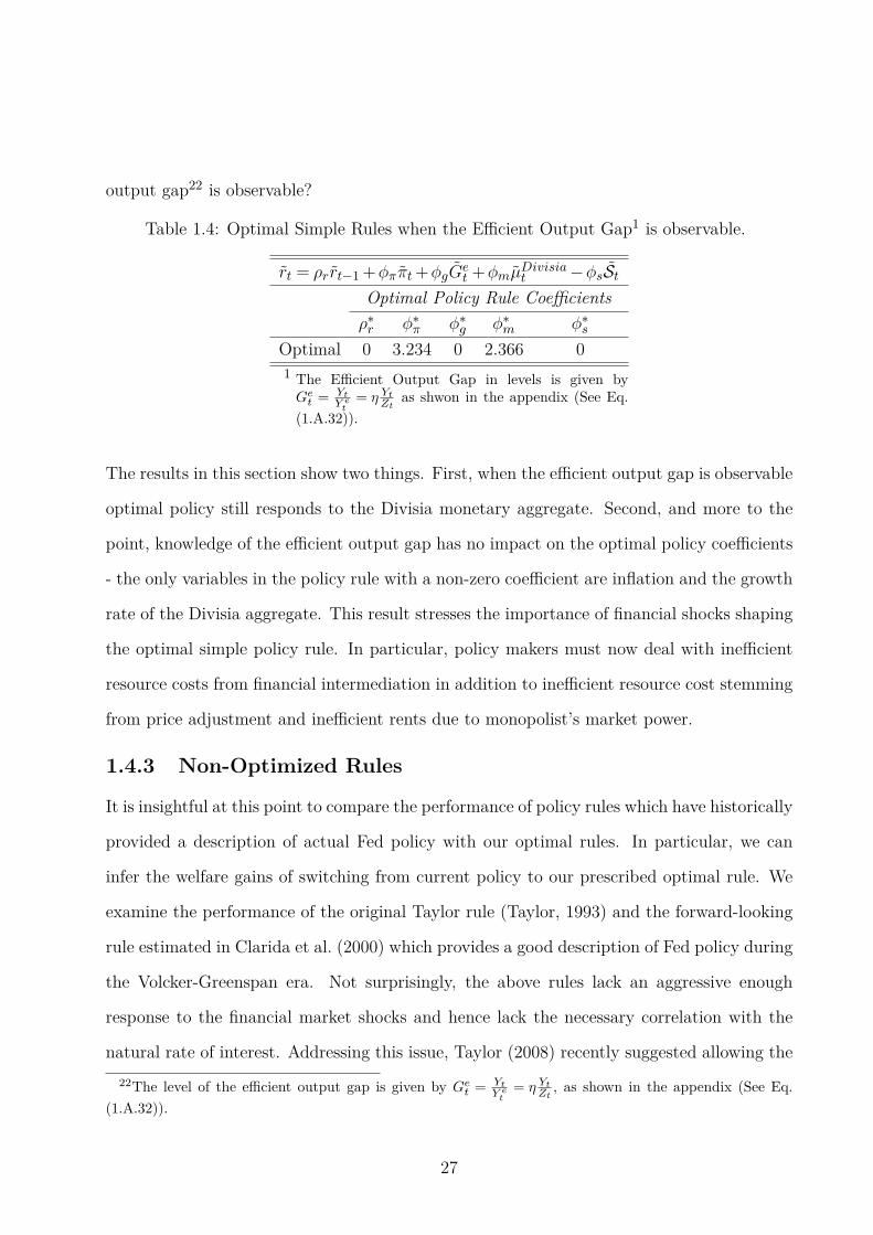
intercept of the Taylor rule to vary with the interest rate spread (SATR). In Table 1.5 we

present the welfare performance of the ad-hoc policy rules.

Table 1.5: Non-Optimized Rules

rt = ρrrt−1 +φπEtπt+i+φgEtGet+i−φsSt

Policy Rule Coefficients Welfare Cost

PolicyRule1 i ρr φπ φg φs Ω2

Taylor Rule 0 0 1.5 .125 0 .2084

CGG3 1 0.79 .4515 .1953 0 .2316

SATR φs = 2 0 0 1.5 .125 2 .3834

1 Here we generalize our previous policy rule allowing for forward(or backward) looking behavior. We use the level of the efficientoutput gap in this rule due to indeterminacy problems when φs > 0associated with the growth rate rule specified in Eq. (1.18).

2 Ω is the % of consumption required to equate welfare under anygiven policy rule to the one under the optimal policy (see Eq.(1.32)). Welfare is calculated as conditional to the initial deter-ministic Ramsey steady state.

3 CGG refers to Clarida, Gali and Gertler’s (2000) estimated forward-looking Taylor rule.

Table 1.6 shows that policy rules which lack a response to financial variables lack correlation

with the natural rate and perform poorly. What is perhaps more shocking is the poor

performance of the SATR - despite bringing about a real policy rate which is highly correlated

with the natural rate of interest. This reiterates our previous point; good policy rules in this

economy are correlated with the natural rate of interest, but correlation with the natural

rate of interest is not sufficient to guarantee good policy.

Table 1.6: Correlation of Real and Natural Interest Rates

Policy Rule Corr(rnt , rt−Etπt+1)

Taylor .1644

CGG .1785

SATR φs = 2 .7269

28

1.4.3.1 Creating liquidity without inflation: Why responding to Money Growth

(Not Interest Rate Spreads) Is Optimal

This poor welfare performance of spread adjusted Taylor rules (SATR) at first seems counter-

intuitive. Table 1.2 suggests countercyclical policy is key to optimally responding to financial

shocks, however the point is bit more subtle. Indeed, responding directly the the interest

rate spread by lowering the policy rate fails to deliver good policy. The reason for this failure

can be seen by examining the impulse responses following a negative banking productivity

shock as shown in Figure 1.2 below. The solid lines show the dynamics under the optimal

policy which reacts to inflation and the Divisia aggregate while the dotted and diamond

lines are the dynamics under various SATR’s. Notice the dynamics for inflation are driven

primarily by the Fisher equation and the monetary policy rule. That is, inflation dynamics

look very similar to the variables in the respective policy rules.

Consider first the interest rate spread rules. A negative banking productivity shock increases

the spread between loan and deposit rates resulting in an immediate cut in the policy rate.

The real rate will rise by more or less depending on the expected behavior of inflation.

Since the rise in the spread has some persistence, the policy rate is expected to remain

below steady state and therefore the inflation rate is expected to remain above steady state

into the future - causing the real policy rate to fall below the nominal policy rate.23 This

amplification of the real rate results in positive output gaps as long as the spread remains

above steady state. More importantly here, the monetary aggregate falls as interest bearing

deposits drop, however the expansionary drop in rates is associated with an increase in the

monetary base - a liquidity effect.

Compared to the optimal policy rule, this uptick in the monetary base under the SATR

is dwarfed. The optimal rule which stabilizes µDivisiat , significantly increases the monetary

base by lowering the real interest rate by more than even the SATR with φs = 10! This

23This affect is more amplified when the shock has more serial correlation. In fact, for larger values of ρx

the nominal rate rises on impact due to the large increase in inflation.

29

2 4 6 8 10 12

−2

0

2

Nominal Policy Rate

2 4 6 8 10 12

−2

0

2

Real Policy Rate

2 4 6 8 10 12−0.5

0

0.5

Inflation

2 4 6 8 10 1290

100

110

Divisia Index Level

2 4 6 8 10 12−20

0

20

Monetary Base

2 4 6 8 10 12

−4

−2

0

Deposits

2 4 6 8 10 120

0.2

0.4

Interest Rate Spread

SATR φS = 10SATR φS = 2Optimal Rule

2 4 6 8 10 12−10

−5

0

Banking Productivity

Figure 1.2: Impulse responses to a negative banking producitivty shock that raises theannualized spread about 25 basis points. All interest rates, the interest rate spread andinflation are in annualized percentage points. All other variables are in % deviations. Thediamond line shows the response under the SATR with φs = 10 and the dotted line showsthe response under the spread adjusted Taylor rule with φs = 2 and the solid line shows theresponse under the optimal simple rule which features a response to inflation and the growthrate of the Divisa index. (See Table 1.1)

increases welfare by providing a substitute for resource intensive financial assets. Moreover,

this increase in the monetary base is accomplished with less inflation volatility than the

SATR. By committing to adjust interest rates as needed to stabilize the growth rate of

the monetary aggregate the central bank is able to create liquidity without large swings in

inflation.

The welfare from the Divisia rule dominates welfare from the spread rule due to the dif-

30

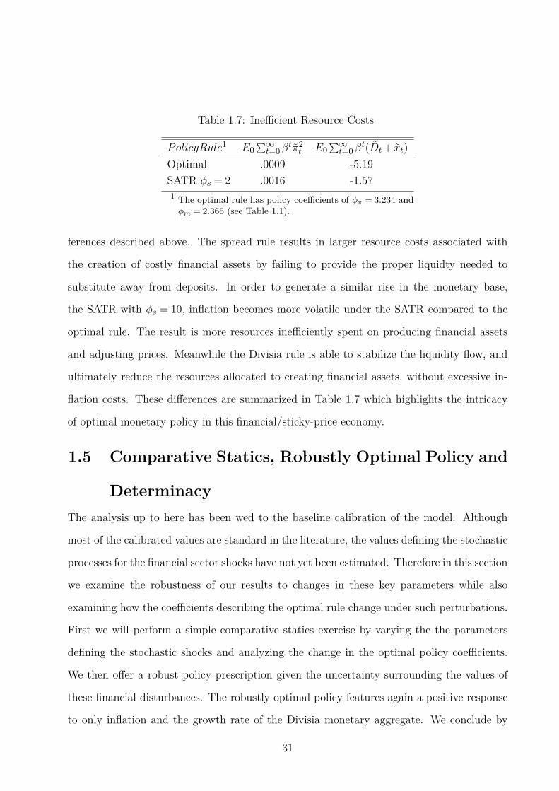
Table 1.7: Inefficient Resource Costs

PolicyRule1 E0∑∞t=0β

tπ2t E0

∑∞t=0β

t(Dt+ xt)

Optimal .0009 -5.19

SATR φs = 2 .0016 -1.57

1 The optimal rule has policy coefficients of φπ = 3.234 andφm = 2.366 (see Table 1.1).

ferences described above. The spread rule results in larger resource costs associated with

the creation of costly financial assets by failing to provide the proper liquidty needed to

substitute away from deposits. In order to generate a similar rise in the monetary base,

the SATR with φs = 10, inflation becomes more volatile under the SATR compared to the

optimal rule. The result is more resources inefficiently spent on producing financial assets

and adjusting prices. Meanwhile the Divisia rule is able to stabilize the liquidity flow, and

ultimately reduce the resources allocated to creating financial assets, without excessive in-

flation costs. These differences are summarized in Table 1.7 which highlights the intricacy

of optimal monetary policy in this financial/sticky-price economy.

1.5 Comparative Statics, Robustly Optimal Policy and

Determinacy

The analysis up to here has been wed to the baseline calibration of the model. Although

most of the calibrated values are standard in the literature, the values defining the stochastic

processes for the financial sector shocks have not yet been estimated. Therefore in this section

we examine the robustness of our results to changes in these key parameters while also

examining how the coefficients describing the optimal rule change under such perturbations.

First we will perform a simple comparative statics exercise by varying the the parameters

defining the stochastic shocks and analyzing the change in the optimal policy coefficients.

We then offer a robust policy prescription given the uncertainty surrounding the values of

these financial disturbances. The robustly optimal policy features again a positive response

to only inflation and the growth rate of the Divisia monetary aggregate. We conclude by

31

0 0.5 1 1.5 2 2.5 3 3.5 4 4.5 50

0.1

0.2

0.3

0.4

0.5

0.6

0.7

0.8

0.9

1

The Welfare Cost of Responding to St

Ω −

Co

st

in %

of

Co

nsu

mp

tio

n

φs

Figure 1.3: St = 1 + (rLt − rDt ) is the gross interest rate spread between loans and deposits(see Eq. (1.11)). The welfare cost Ω are relative to the optimal policy (see Table 1.1). Aswe vary φs we keep φπ = 1.5 and φg = .125 as in the original Taylor rule (Taylor, 1993).

examining determinacy properties of this rule - a point of practical concern for policy makers.

We show the reaction to Divisia compliments the reaction to inflation, so far as determinacy

is concerned, resulting in a novel Taylor principle for monetary aggregates.

1.5.1 Comparative Statics

In much the spirit of Poole (1970) we examine how the optimal policy coefficients change

when the shocks driving the economy change. We find that when the standard deviation

of financial shocks increase, the optimal response to the monetary aggregate increases as

32

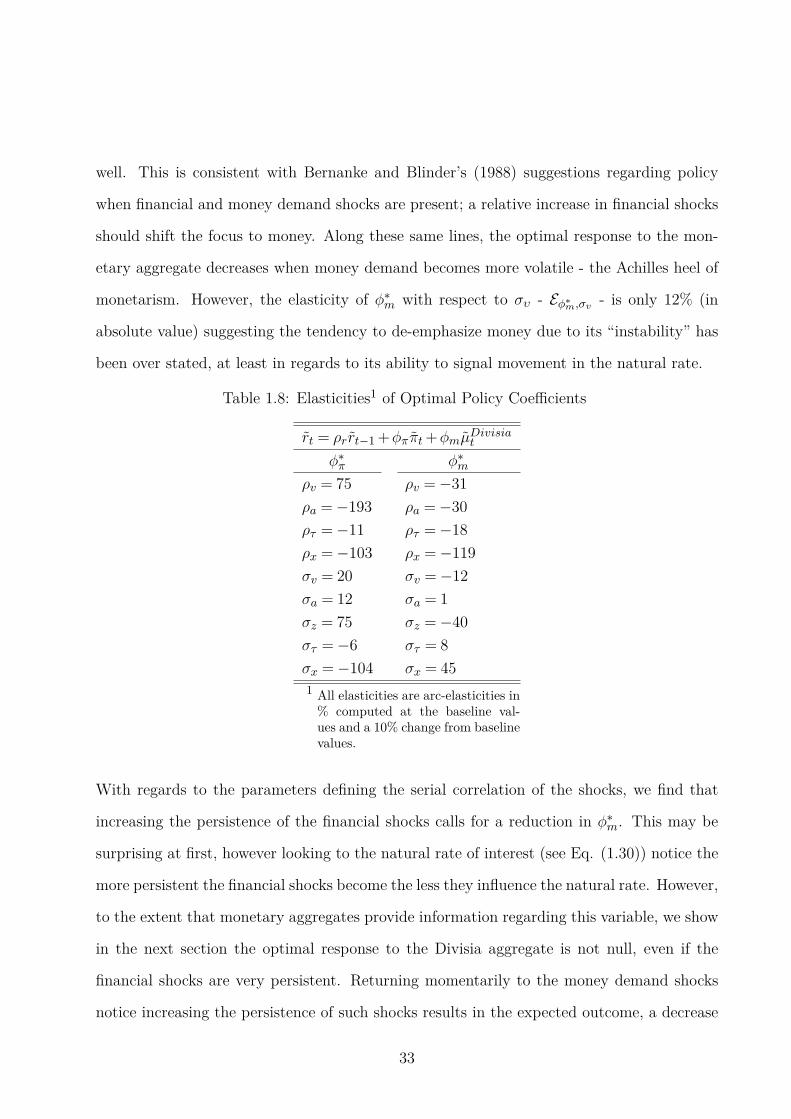
well. This is consistent with Bernanke and Blinder’s (1988) suggestions regarding policy

when financial and money demand shocks are present; a relative increase in financial shocks

should shift the focus to money. Along these same lines, the optimal response to the mon-

etary aggregate decreases when money demand becomes more volatile - the Achilles heel of

monetarism. However, the elasticity of φ∗m with respect to συ - Eφ∗

m,σv- is only 12% (in

absolute value) suggesting the tendency to de-emphasize money due to its “instability” has

been over stated, at least in regards to its ability to signal movement in the natural rate.

Table 1.8: Elasticities1 of Optimal Policy Coefficients

rt = ρrrt−1 +φππt+φmµDivisiat

φ∗π φ∗

m

ρv = 75 ρv = −31

ρa = −193 ρa = −30

ρτ = −11 ρτ = −18

ρx = −103 ρx = −119

σv = 20 σv = −12

σa = 12 σa = 1

σz = 75 σz = −40

στ = −6 στ = 8

σx = −104 σx = 45

1 All elasticities are arc-elasticities in% computed at the baseline val-ues and a 10% change from baselinevalues.

With regards to the parameters defining the serial correlation of the shocks, we find that

increasing the persistence of the financial shocks calls for a reduction in φ∗m. This may be

surprising at first, however looking to the natural rate of interest (see Eq. (1.30)) notice the

more persistent the financial shocks become the less they influence the natural rate. However,

to the extent that monetary aggregates provide information regarding this variable, we show

in the next section the optimal response to the Divisia aggregate is not null, even if the

financial shocks are very persistent. Returning momentarily to the money demand shocks

notice increasing the persistence of such shocks results in the expected outcome, a decrease

33

in φ∗m. Again though, this effect is relatively small as Eφ∗

m,σvis only about 30%.

1.5.2 Robustly Optimal Policy

The previous section highlights the fact that the exact coefficients that define the optimal

policy rule depend on the underlying stochastic processes. Hence, one may wonder then,

given our uncertainty over such parameters what is the best policy to follow? We will

provide a first attempt to answer this question using a simple 2 player game zero-sum game.

In particular, following Giannoni (2002), we set up the zero-sum game Γ between the central

bank (CB) and nature (N). The central bank would like to choose policy rule parameters

- φ ∈ Φ - to maximize welfare defined by W0 (see Eq. (4.2)). At the same time, nature is

malevolent and would like to choose shock parameters - σ ∈ Σ - which minimize W0. The

Nash equilibrium represents the worst set of structural parameters possible, given policy

makers choose the best possible policy given the bad state of the world. Intuitively, the

Nash equilibrium of this game provides a policy prescription that does the best under the

worst case scenario. The nature of zero-sum games allows us to consider solving the minimax

problem to find the Nash equilibrium

minφ∈Φ

maxσ∈Σ

−W0

We numerically approach a solution by iterating over natures problem and over the policy

makers problem until all parameters and the objective function converge.

Before solving this problem we must set bounds on the choice space of nature. For the

money demand, preference and technology process we assume all parameters lie within 2

standard errors using the estimates from Ireland (2004a) with an upper bound of .99 for the

persistence parameters24. Unfortunately, the parameters driving the financial shocks have no

comparable estimates to help determine an appropriately bounded set. Therefore we assume

that ρx ∈ [0, .99] and ρτ ∈ [0, .99]. As for the standard deviations of these shocks we continue

24As with the rest of the paper, we continue to assume a unit-root in the technology shock

34

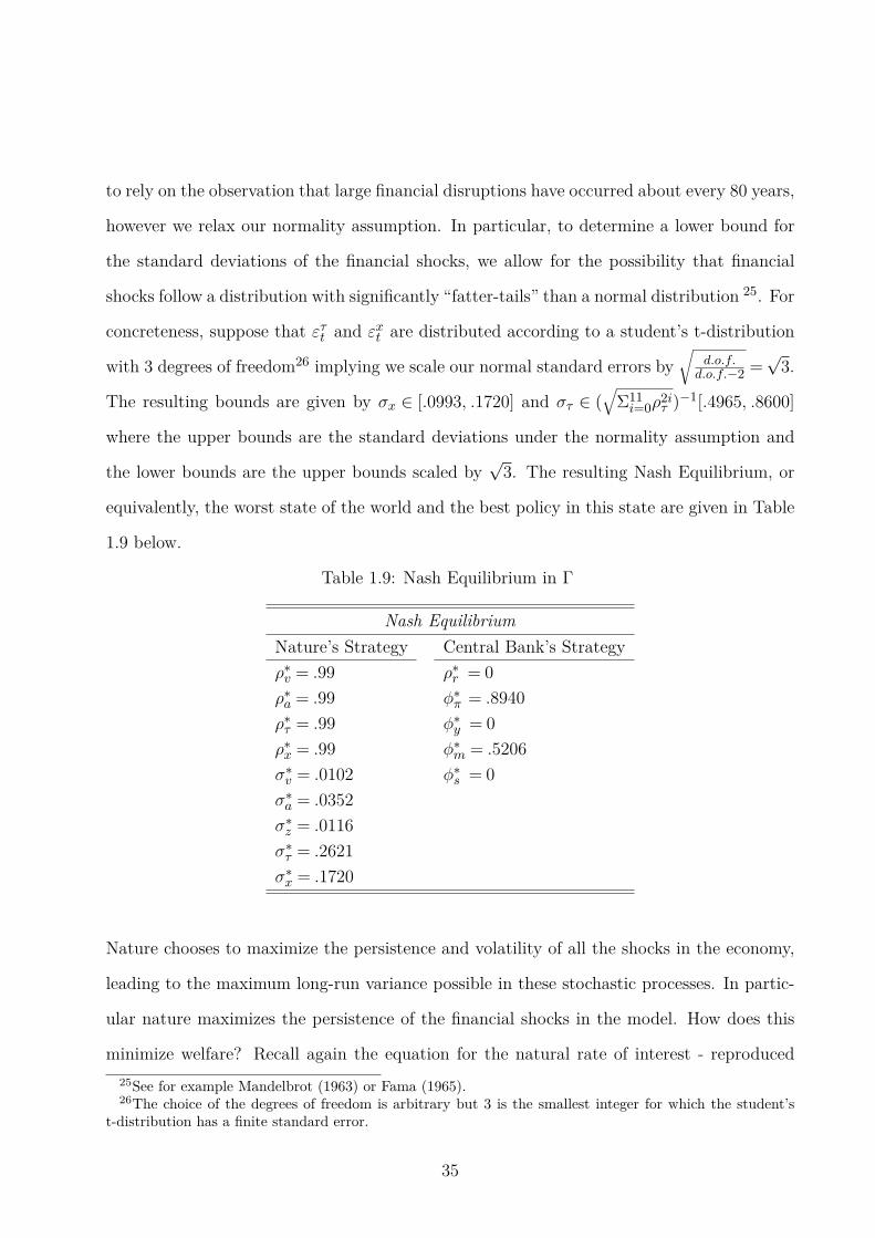
to rely on the observation that large financial disruptions have occurred about every 80 years,

however we relax our normality assumption. In particular, to determine a lower bound for

the standard deviations of the financial shocks, we allow for the possibility that financial

shocks follow a distribution with significantly “fatter-tails” than a normal distribution 25. For

concreteness, suppose that ετt and εxt are distributed according to a student’s t-distribution

with 3 degrees of freedom26 implying we scale our normal standard errors by√

d.o.f.d.o.f.−2 =

√3.

The resulting bounds are given by σx ∈ [.0993, .1720] and στ ∈ (√

Σ11i=0ρ

2iτ )−1[.4965, .8600]

where the upper bounds are the standard deviations under the normality assumption and

the lower bounds are the upper bounds scaled by√

3. The resulting Nash Equilibrium, or

equivalently, the worst state of the world and the best policy in this state are given in Table

1.9 below.

Table 1.9: Nash Equilibrium in Γ

Nash Equilibrium

Nature’s Strategy Central Bank’s Strategy

ρ∗v = .99 ρ∗

r = 0

ρ∗a = .99 φ∗

π = .8940

ρ∗τ = .99 φ∗

y = 0

ρ∗x = .99 φ∗

m = .5206

σ∗v = .0102 φ∗

s = 0

σ∗a = .0352

σ∗z = .0116

σ∗τ = .2621

σ∗x = .1720

Nature chooses to maximize the persistence and volatility of all the shocks in the economy,

leading to the maximum long-run variance possible in these stochastic processes. In partic-

ular nature maximizes the persistence of the financial shocks in the model. How does this

minimize welfare? Recall again the equation for the natural rate of interest - reproduced

25See for example Mandelbrot (1963) or Fama (1965).26The choice of the degrees of freedom is arbitrary but 3 is the smallest integer for which the student’s

t-distribution has a finite standard error.

35

here for convenience.

rnt = (1−ρa)at− (1−ρz)Zt−Ψrn

x (1−ρx)xt−Ψrn

τ (1−ρτ )τt

By pushing the persistence of the financial shocks to their maximum, nature is trying to

mitigate the financial shocks role in driving the natural rate. Why? When financial shocks

affect the natural rate policy makers reacting to the Divisia aggregate are able to correlate

the real rate with the natural rate. However, by limiting the share of variance in the natural

rate explained by financial shocks, while at the same time maximizing the long-run variance

of money demand shocks, nature is effectively maximizing the noise to signal ratio of Divisia

in signaling movements in the natural rate. Interestingly though welfare is still improved by

including a positive - but weakened - reaction to the Divisia aggregate. Therefore, much in

line with Brainard’s (1967) seminal work on policy under uncertainty we find (in contrast

to Giannoni (2002)) uncertainty calls for an attenuated reaction to both inflation and the

monetary aggregate. However the Divisia response is significant - even in this extreme state

of the world.

1.5.3 Determinacy

Thus far we have found the optimal simple and robust rules feature a positive response

to only inflation and the Divisia monetary aggregate. Clearly if the aforementioned policy

rules are followed “to the letter” then the outcome is determinate in the sense that there

is a unique path for all nominal and real variables. However, a practical concern for policy

makers faced with the policy prescription in this economy is whether reacting to the Divisia

monetary aggregate induces undesirable equilibrium outcomes that an inflation only rule

would preclude. In other words, if policy deviates slightly from the prescribed rule is the

equilibrium outcome still unique? To answer this question we examine the determinacy

properties of the optimal rule in this economy. Unfortunately, analytical solutions are not

available as in Bullard & Mitra (2002) so instead we examine the determinacy properties

36

of this rule numerically. We examine determinacy by searching over the values φπ ∈ [0,5]

and φm ∈ [0,5] by .01 increments and and ρr ∈ [0,1) by .1 increments around both the

steady state of the competitive equilibrium and the Ramsey steady state and examining the

necessary and sufficient condition for existence and uniqueness as laid out by Blanchard &

Kahn (1980). The resulting determinacy region is featured in Figure 1.4.

0 0.5 1 1.5 2 2.5 3 3.5 4 4.5 50

0.5

1

1.5

2

2.5

3

3.5

4

4.5

5

φπ

φ m

Determinacy Region Underrt = ρr rt−1 + φππt + φmµDivisia

t

ρr→1

Determinateρ

r=0

Figure 1.4: The shadded area to the northeast of the dotted line, defined by φm +φπ > 1,is determinate when ρr = 0. Moreover, if ρr > 0 then the condition for determinacy underthis rule generalizes to φm+φπ

1−ρr> 1, this is a genralized Taylor principle for Divisia monetary

aggregates in interest rate rules.

Looking first along the horizontal axis where φm = 0, the well known Taylor principle con-

37

tinues to hold. That is policy makers can guarantee a unique equilibrium by satisfying

φπ > 1

Moreover, looking at the vertical axis where φπ = 0, we find that policy makers can guarantee

a unique equilibrium outcome by adjusting the policy rate more than one for one with changes

in the growth rate of the Divisia monetary aggregate27. That is, the condition that

φm > 1

is sufficient for determinacy. However, our optimal simple and robust rules feature a positive

response to both inflation and the Divisia monetary aggregate. Therefore, focusing our

attention on the interior Figure 4, where both responses are positive, we find that the above

two conditions are sufficient but clearly not necessary as determinacy is more generally

possible by satisfying the condition

φπ +φm > 1 (1.33)

Reacting to the growth rate of Divisia actually allows policy makers to achieve determinacy

with even weaker inflation responses so long as the reaction to Divisia is increased one for

one. Equation (1.33) provides an extension of the well-known Taylor principle to Taylor

rules featuring a response to the Divisia monetary aggregate - a modified Taylor principle

for Divisia monetary aggregates. Most generally, if policy makers introduce lagged interest

rates into the policy rule we see that condition (1.33) generalizes to

φπ +φm1−ρr

> 1 (1.34)

27We emphasize this result is not generally true for any monetary aggregate. In fact, we show in theappendix embedding the simple-sum monetary aggregate (see Eq. (1.22)) tends to result in indeterminacyand no such modified Taylor principle holds.

38

Equations (1.33) and (1.34) show that there are no more concerns regarding determinacy

under optimal rules in this model than there are regarding determinacy in standard NKSP

where φm = 0 and in fact determinacy is more likely when reacting to the Divisia monetary

aggregate.

1.6 Conclusion

We have analyzed optimal monetary policy in a NKSP augmented to include a financial

sector. We showed financial disturbances which decrease banks ability and willingness to

produce financial assets lowers the natural rate of interest calling for countercyclical monetary

policy. The resulting optimal policy deviates from the common inflation only type of Taylor

rule common in this literature. Instead, reacting to the growth rate of the Divisia monetary

aggregate, in addition to inflation, performs significantly better than reacting to inflation

alone. The resulting policy rule produces a real interest rate which is highly correlated with

the natural rate of interest. We showed the spread adjusted Taylor rule as advocated by

Taylor (2008) actually performs worse than inflation only rules despite its high correlation

with the natural rate of interest. This puzzling result is reconciled by the increased inflation

and output gap volatility induced by the spread adjusted Taylor rules which is not present

in the Divisia growth rules. The optimality of reacting positively to the Divisia growth rate

and the inflation rate is shown to hold under different assumption regarding policy maker’s

information sets and preferences over monetary assets. Finally, we offer a robust policy

prescription under parametric uncertainty using the minimax approach proposed in Giannoni

(2002). The resulting policy rule features an attenuated - but positive and economically

significant - response to the growth rate of Divisia and inflation. Moreover, we offer some

insight regarding the ability of such rules to bring about a unique equilibrium outcome by

examining their determinacy region. The result is a modified Taylor principle for Divisia

monetary aggregate which is sufficient to guarantee determinacy.

As much as the seminal work of Taylor (1993) marked the beginning of interest rate rules

39

dominating monetary policy we hope this paper can be part of the beginning of re-examining

the usefulness of monetary aggregates in real time policy making. Given the interest in sim-

ple rules and macro policy under financial distress considerable work lies ahead in better

understanding how policy makers can better use the information available in monetary ag-

gregates and other variables available in real time. Specifically, one may wonder in our

environment if Divisia level targeting is superior to reacting to the growth rate of the Divisia

monetary aggregate. Also, expanding the literature on statistical index number theory to

properly track aggregate quantities of credit seems a worthwhile task given the usefulness of

properly constructed monetary aggregates in this model. Furthermore, the zero-lower bound

on nominal interest rates suggests the usefulness of monetary aggregates may extend beyond

informational variables to policy instruments as called for by Taylor (2009). However, an

optimal policy prescription for monetary instrument rules is seriously lacking in this modern

framework due to the exclusive focus on interest rates. This calls for future work to under-

stand how different aggregates perform as instruments from their determinacy properties to

their welfare performance.

40

References

Andres, J., Lopez-Salido, J. D., & Nelson, E. (2009). Money and the natural rate of inter-

est: Structural estimates for the united states and the euro area. Journal of Economic

Dynamics and Control, 33(3), 758–776.

Barnett, W. A. (1978). The user cost of money. Economics Letters, 1(2), 145–149.

Barnett, W. A. (1980). Economic monetary aggregates an application of index number and

aggregation theory. Journal of Econometrics, 14(1), 11–48.

Barnett, W. A. (2012). Getting it Wrong: How Faulty Monetary Statistics Undermine the

Fed, the Financial System, and the Economy, volume 1 of MIT Press Books. The MIT

Press.

Barnett, W. A. & Chauvet, M. (2011a). Financial Aggregation And Index Number Theory,

volume 2 of World Scientific Books. World Scientific Publishing Co. Pte. Ltd.

Barnett, W. A. & Chauvet, M. (2011b). How better monetary statistics could have signaled

the financial crisis. Journal of Econometrics, 161(1), 6–23.

Barnett, W. A. & Serletis, A. (2000). The Theory of Monetary Aggregation. Contributions

to Economic Analysis. Elsevier.

Barnett, W. A. & Singleton, K. J. (1987). The microeconomic theory of monetary aggregation.

Cambridge University Press.

41

Belongia, M. T. (1996). Measurement matters: Recent results from monetary economics

reexamined. Journal of Political Economy, 104(5), 1065–83.

Belongia, M. T. & Binner, J. M. (2000). Divisia Monetary Aggregates: Theory and Practice.

Palgrave.

Belongia, M. T. & Ireland, P. N. (2006). The own-price of money and the channels of

monetary transmission. Journal of Money, Credit and Banking, 38(2), 429–445.

Belongia, M. T. & Ireland, P. N. (2013). The barnett critique after three decades: A new

keynesian analysis. Journal of Econometrics, forthcoming.

Berger, H. & Weber, H. (2012). Money as Indicator for the Natural Rate of Interest. IMF

Working Papers 12/6, International Monetary Fund.

Bernanke, B. S. & Blinder, A. S. (1988). Credit, money, and aggregate demand. American

Economic Review, 78(2), 435–39.

Blanchard, O. J. & Kahn, C. M. (1980). The solution of linear difference models under

rational expectations. Econometrica, 48(5), 1305–11.

Brainard, W. (1967). Uncertainty and the effectiveness of policy. American Economic Review,

57(2), 411–425.

Bullard, J. & Mitra, K. (2002). Learning about monetary policy rules. Journal of Monetary

Economics, 49(6), 1105–1129.

Clarida, R., Gali, J., & Gertler, M. (2000). Monetary policy rules and macroeconomic

stability: Evidence and some theory. The Quarterly Journal of Economics, 115(1), 147–

180.

Curdia, V. & Woodford, M. (2009). Credit frictions and optimal monetary policy. BIS

Working Papers 278, Bank for International Settlements.

42

Curdia, V. & Woodford, M. (2010). Credit spreads and monetary policy. Journal of Money,

Credit and Banking, 42(s1), 3–35.

Dellas, H., Diba, B., & Loisel, O. (2010). Financial Shocks and Optimal Policy. Technical

report.

Diewert, W. E. (1976). Exact and superlative index numbers. Journal of Econometrics,

4(2), 115–145.

Faia, E. & Monacelli, T. (2007). Optimal interest rate rules, asset prices, and credit frictions.

Journal of Economic Dynamics and Control, 31(10), 3228–3254.

Fama, E. F. (1965). The behavior of stock-market prices. The Journal of Business, 38(1),

pp. 34–105.

Gali, J. (2008). Monetary Policy, Inflation, and the Business Cycle: An Introduction to the

New Keynesian Framework. Princeton University Press.

Gali, J., Lopez-Salido, J. D., & Valles, J. (2003). Technology shocks and monetary policy:

assessing the fed’s performance. Journal of Monetary Economics, 50(4), 723–743.

Giannoni, M. P. (2002). Does model uncertainty justify caution? robust optimal monetary

policy in a forward-looking model. Macroeconomic Dynamics, 6(01), 111–144.

Ireland, P. N. (2000). Interest rates, inflation, and federal reserve policy since 1980. Journal

of Money, Credit and Banking, 32(3), 417–34.

Ireland, P. N. (2004a). Money’s role in the monetary business cycle. Journal of Money,

Credit and Banking, 36(6), 969–83.

Ireland, P. N. (2004b). Technology shocks in the new keynesian model. The Review of

Economics and Statistics, 86(4), 923–936.

43

Ireland, P. N. (2011). The Macroeconomic Effects on Interest on Reserves. Boston College

Working Papers in Economics 772, Boston College Department of Economics.

Kim, H., Kim, J., Schaumburg, E., & Sims, C. A. (2005). Calculating and Using Second

Order Accurate Solutions of Discrete Time Dynamic Equilibrium Models. Technical report.

Kydland, F. E. & Prescott, E. C. (1982). Time to build and aggregate fluctuations. Econo-

metrica, 50(6), 1345–70.

Lombardo, G. & Vestin, D. (2008). Welfare implications of calvo vs. rotemberg-pricing

assumptions. Economics Letters, 100(2), 275–279.

Mandelbrot, B. (1963). The variation of certain speculative prices. The Journal of Business,

36, 394.

McCallum, B. T. & Nelson, E. (2011). Money and inflation: Some critical issues. In B. M.

Friedman & M. Woodford (Eds.), Handbook of Monetary Economics, volume 3 of Handbook

of Monetary Economics chapter 3, (pp. 97–153). Elsevier.

Orphanides, A. (2003). The quest for prosperity without inflation. Journal of Monetary

Economics, 50(3), 633–663.

Poole, W. (1970). Optimal choice of monetary policy instruments in a simple stochastic

macro model. The Quarterly Journal of Economics, 84(2), 197–216.

Rotemberg, J. J. (1982). Sticky prices in the united states. Journal of Political Economy,

90(6), 1187–1211.

Schmitt-Grohe, S. & Uribe, M. (2004). Solving dynamic general equilibrium models using

a second-order approximation to the policy function. Journal of Economic Dynamics and

Control, 28(4), 755–775.

Schmitt-Grohe, S. & Uribe, M. (2007). Optimal simple and implementable monetary and

fiscal rules. Journal of Monetary Economics, 54(6), 1702–1725.

44

Schmitt-Grohe, S. & Uribe, M. (2012). An ols approach to computing ramsey equilibria in

medium-scale macroeconomic models. Economics Letters, 115, 128–129.

Taylor, J. B. (1993). Discretion versus policy rules in practice. Carnegie-Rochester Confer-

ence Series on Public Policy, 39(1), 195–214.

Taylor, J. B. (2008). Monetary Policy and the State of the Economy. Testimony before the

committee on financial services u.s. house of representatives.

Taylor, J. B. (2009). The need to return to a monetary framework. Business Economics,

44(2), 63–72.

Woodford, M. (2003). Interest and Prices: Foundations of a Theory of Monetary Policy.

Princeton University Press.

45

1.A Appendix: The Equilibrium System

In this portion of the appendix we derive the model’s equilibrium conditions and stationarizethe model allowing us to define a recursive (imperfectly) competitive equilibrium. We alsoderive expressions for the natural rate level of output and the natural interest rate.

1.A.1 The Representative Household’s FOCS

Non-Separable Preferences: First consider the case when monetary assets are not additivelyseparable from consumption. In particular, recall from section 2.1.3 that the household facesthe following problem when preferences over monetary assets are defined according to ashopping time friction;

maxCt,ht,MA

t ,Nt,Dt,Lt,Bt+1,Mt+1,st+1(i)∞t=0

E0

∞∑

t=0

βtat [ln(Ct)−η(ht+hst )]

subject to (3.1), (1.2), (1.3) and (1.4) taking B0, M0 and s0(i) as given. After substituting(1.4) into the objective function, we can form the Bellman equation as follows where all theconstraints are expressed in real terms by dividing through by Pt,

V (Bt−1,Mt−1, st−1(i)) =max

at

[

ln(Ct)−ηht−η

χ

(

υtPtCt

MAt

)χ ]

−Λ1t

Dt−Mt−1 −Bt−1 +

´ 10 Qt(i)(st(i)− st−1(i))di+Bt/rt+Nt−Lt

Pt

−Λ2t

MAt

Pt−[

ν1ω (NtPt

)ω−1

ω +(1−ν)1ω (Dt

Pt)

ω−1ω

] ωω−1

−Λ3t

Mt−Nt+PtCt−Wtht−

´ 10 Ft(i)st(i)di− rDt Dt+ rLt LtPt

+βEt[V (Bt,Mt, st(i))]

The first order necessary conditions are given by the following equations. The system of

equations (1.A.1)-(1.A.9) is under-determined in the sense that we have introduced various

derivatives of the value function. However, we can complement these first order necessary

conditions with the Bienveniste-Scheinkman Envelope Conditions to eliminate the value

function from the system above. These envelope conditions are given in equations (1.A.10)-

(1.A.12) below.

46

at

[

1−η

(

υtPtCt

MAt

)χ]

−Λ3tCt = 0 (1.A.1)

−atη+Λ3tWt

Pt= 0 (1.A.2)

ηat

(

υtPtCt

MAt

)χ

− Λ2tM

At

Pt= 0 (1.A.3)

(Dt

Pt

)

− (1−ν)

(

MAt

Pt

)[

Λ2t

Λ1t −Λ3

t rDt

]ω

= 0 (1.A.4)

(NtPt

)

−ν

(

MAt

Pt

)[

Λ2t

Λ1t −Λ3

t

]ω

= 0 (1.A.5)

Λ1t −Λ3

t rLt = 0 (1.A.6)

−Λ1t

rt+PtβEt[V

′

Bt(Bt,Mt, st(i))] = 0 (1.A.7)

−Λ3t +PtβEt[V

′

Mt(Bt,Mt, st(i))] = 0 (1.A.8)

−Λ1tQt(i)+Λ3

tFt(i)+PtβEt[V′

st(i)(Bt,Mt, st(i))] = 0 (1.A.9)

Envelope Conditions:

V′

Bt−1(Bt−1,Mt−1, st(i)) =

Λ1t

Pt(1.A.10)

V′

Mt−1(Bt−1,Mt−1, st(i)) =

Λ1t

Pt(1.A.11)

V′

st−1(i)(Bt−1,Mt−1, st(i)) =Λ1tQt(i)

Pt(1.A.12)

Now update (1.A.10)-(1.A.12) and substitute the resulting equations into (1.A.6)-(1.A.8)

yielding:

47

−Λ1t

rt+βEt

[

PtΛ1t+1

Pt+1

]

= 0 (1.A.13)

−Λ3t +βEt

[

PtΛ1t+1

Pt+1

]

= 0 (1.A.14)

−Λ1tQt(i)

Pt+Λ3

tFt(i)

Pt+βEt

[

Λ1t+1Qt+1(i)

Pt+1

]

= 0 (1.A.15)

The conditions (1.A.1)-(1.A.6) and (1.A.13)-(1.A.15) define the consumers optimal behavior.

Separable Preferences: Under additively separable preferences over monetary assets the

household’s first order conditions are identical to the above conditions after replacing (1.A.1)

and (1.A.3) with

atCt

−Λ3t = 0 (1.A.16)

ηmatυt−Λ2tMAt

Pt= 0 (1.A.17)

respectively.

1.A.2 Deriving the User Costs of Monetary Assets

As shown in an infinite planning horizon by Barnett & Singleton (1987), we can derive the

user costs of all monetary assets in the model from the household’s first order necessary

conditions. Specifically, the user costs appear naturally as the price of monetary assets

according to the familiar optimality condition from microeconomics which dictates, at an

optimum, equating the marginal rate of substitution of currency for deposits to the ratio of

the price of currency to the price of deposits.

∂ut∂Nt

∂ut∂Dt

=

∂ut

∂MAt

∂MAt

∂Nt

∂ut

∂MAt

∂MAt

∂Dt

=

Λ1t −Λ3

t

Λ2t

Λ1t −Λ3

t rDt

Λ2t

=Λ3t rLt −Λ3

t

Λ3t rLt −Λ3

t rDt

=rLt −1

rLt − rDt≡ uNtuDt

48

The second equality follows from equations (1.A.4) and (1.A.5), the household’s first order

conditions for Nt and Dt. The third equality follows from equation (1.A.6), the household’s

first order condition for Lt. The resulting ratio defines the relative user costs.

We can also derive the exact price dual to the true quantity aggregator in a similar fashion.

Instead of considering the price of each monetary assets individually, consider the optimality

condition the monetary aggregate must satisfy. For simplicity, consider the marginal rate of

substitution of the monetary aggregate for consumption. Clearly the price of the consump-

tion good is Pt, hence the numerator must denote the price of the monetary aggregate.

∂ut

∂MAt

∂ut∂Ct

=

Λ2tPt

Λ3t

=

Λ2t

Λ3t

Pt=

[

ν(rt−1)(1−ω) +(1−ν)(rt− rDt )(1−ω)] 1

1−ω

Pt≡ rLt − rAt

Pt

uAt = rLt − rAt =[

ν(rt−1)(1−ω) +(1−ν)(rt− rDt )(1−ω)] 1

1−ω (1.A.18)

The first equality follows from equations (1.A.1) and (1.A.3), the household’s first order con-

ditions for Ct and MAt respectively. The third equality follows from solving equation (1.A.4)

for Nt, equation (1.A.5) for Dt and substituting the resulting expressions into equation (1.3).

The resulting expression can be solved for Λ2t

Λ3t

yielding the numerator the follows the third

equality. For the last equality we define this expression to be rt−rAt , or the opportunity cost

of holding the aggregate monetary asset MAt . The resulting aggregate user cost (1.A.18)

as defined by Barnett (1978) is of the same form as the individual component user costs in

equations (1.20) and (1.21). It can be verified that (1.A.18) is in fact the true price dual to

the true monetary aggregate in equation (1.3) since it satisfies Fisher’s factor reversal test.

MAt u

At = uNt Nt+uDt Dt (1.A.19)

Equation (1.A.19) states that the true quantity index times the true price index equals total

expenditures, in this sense, (1.A.18) is the exact price dual to (1.3).

49

1.A.3 Equilibrium Quantity of the Monetary Aggregate

In this section we derive a condition relating the monetary aggregate to output, a vector

of interest rates and financial shocks. This expression is useful for deriving the natural

rates of output and interest later and also because it highlights the difference between broad

money which depends on a vector of interest rates and the financial sector’s productive

ability versus typical “money demand” specifications which assume the equilibrium quantity

of money depends only agents demand for monetary assets featuring a single interest rate.

All variables with a tilde denote the real detrended variable in log-deviations from steady

state (with the exception of interest rates which are in nominal terms). Combine (1.A.2),

(1.A.3) (or (1.A.16), (1.A.17)) and (1.A.18) to arrive at (up to additive constants)

MAt = γcmCt+γwmWt−γu

A

m uAt +γυmυt (1.A.20)

where under additively separable preferences γcm = γuA

m = γυm = 1, andγwm = 0 and under non-

additively separable preferences γcm = γυm = χ1+χ , andγ

wm = γu

A

m = 11+χ . Now log-linearize the

household’s first order condition relating the real wage to the marginal utilities of consump-

tion and leisure and we have that

Wt = (1+γm)Ct−γmMAt +γmυt (1.A.21)

where γm =u

′′

MA,C

u′

C

is zero for additively separable preferences. Now substitute (1.A.21) into

(1.A.20) to eliminate the real wage and arrive at

MAt =

[γcm+γwm(1+γm)]

[1+γwmγm]Ct−

γuA

m

[1+γwmγm]uAt +

[γwmγm+γυm]

[1+γwmγm]υt (1.A.22)

50

We can express consumption in terms of output and the monetary aggregate by substituting

equation (1.A.5) into equation (3.28) and log-linearizing to arrive at

Ct =1

sc

[

Yt− (1− sc)[

xt+MAt +ω

(

uAt − uDt)]]

(1.A.23)

where sc = CY

. Our equilibrium condition for the monetary aggregate is obtained by sub-

stituting (1.A.23) into (1.A.22) and noting that under either specification of preferences

γcm+γwm = 1

MAt = Yt−ηuAuAt +ηuD uDt +ηυυt−ηxxt (1.A.24)

where

ηuA = (1− sc)ω+γu

A

m sc(1+γmγwm)

ηuD = ω(1− sc)

ηυ = sc

(

1− 1−γυm1+γmγwm

)

ηx = (1− sc)

and all the coefficients are positive.

1.A.4 The Representative Intermediate Goods Firm’s FOCS

Recall from section 2.4, the representative intermediate goods producing firm i ∈ [0,1] max-

imizes its share price in every period t= 0,1,2,3, .... Mathematically, we have

maxht(i),Pt(i)∞

t=0

Qt(i)

Ptsubjectto(1.14)and(1.15).

To derive the first order necessary conditions for this problem use the equity pricing rela-

tionship (1.A.15) from the representative household’s first order condition to solve for period

t. Solving (1.A.15) forward and assuming no bubbles yields

51

Qt(i)

Pt= Et

∞∑

j=0

βjΛ3t+jFt+j(i)

Λ1tPt+j

. (1.A.25)

Equation (1.A.25) is a familiar asset pricing relationship which states that the market share

price of the representative intermediate goods producing firm is proportional to the expected

future stream of dividends adjusted for risk. In particular, the stochastic discount factor is

given byβjΛ3

t+j

Λ1t. In any period t = 0,1,2,3, ..., intermediate goods producing firm i ∈ [0,1]

pays out all profits as dividends. In real terms, the period t real dividend is given by

Ft(i)

Pt=Pt(i)

PtYt(i)− Wt

Ptht(i)− φ

2

[

Pt(i)

Pt−1(i)π−1

]2

Yt. (1.A.26)

The first term of the above profit function is period t real revenue, the second term in the

firm’s period t real wage bill and the third term will be 0 unless the intermediate goods

producing firm changes its price from period t− 1 to period t an amount different than

the steady-state gross rate of inflation rate, π. Substituting (1.A.26) into (1.A.25), we can

restate the intermediate goods producing firm’s problem as

maxht(i),Pt(i)∞

t=0

E0

∞∑

t=0

βtΛ3t

Λ10

Pt(i)

PtYt(i)− Wt

Ptht(i)− φ

2

[

Pt(i)

Pt−1(i)π−1

]2

Yt

subject to

Yt(i) =

[

Pt(i)

Pt

]−θ

Yt and Yt(i) = ztht(i).

The problem can be simplified by substituting the inverse of the technology constraint for

ht(i) and then substituting the factor demand into the resulting expression for Yt(i) so

that now the representative intermediate goods producing firm solves the following recursive

problem defined by Bellman’s equation

52

V (Pt−1(i)) = maxPt(i)

Λ3tYtΛ1

0

[

Pt(i)

Pt

]1−θ

− Wt

Ptzt

[

Pt(i)

Pt

]−θ

− φ

2

[

Pt(i)

Pt−1(i)π−1

]2

+βEt[V (Pt)]

The first order necessary condition for the problem is given by

(1− θ)Λ3tYtΛ1

0

[

Pt(i)

Pt

]−θ1

Pt+ θ

Λ3tYtΛ1

0

Wt

P 2t zt

[

Pt(i)

Pt

]−1−θ

−φΛ3tYtΛ1

0

[

Pt(i)

Pt−1(i)π−1

]

1

Pt−1(i)π+βEt[V

′

(Pt)] = 0 (1.A.27)

Once again invoking the Bienveniste-Scheinkman Envelope Condition we have

V′

(Pt−1(i)) =Λ3tYtΛ1

0

φ

[

Pt(i)

Pt−1(i)π−1

]

Pt(i)

(Pt−1(i))2π. (1.A.28)

Updating (1.A.28) one period and substituting into (1.A.27) and then multiplying the re-

sulting equation by Λ10Pt yields

(1− θ)

[

Pt(i)

Pt

]−θ

+ θWt

Ptzt

[

Pt(i)

Pt

]−1−θ

−φ

[

Pt(i)

Pt−1(i)π−1

]

PtPt−1(i)π

+βφEt

[

Λ3t+1Yt+1

Λ3tYt

[

Pt+1(i)

Pt(i)π−1

]

PtPt+1(i)

(Pt(i))2π

]

= 0 (1.A.29)

Finally, when (1.A.29) is log-linearized around a symmetric equilibrium where Pt(i) =Pt ∀ t=

0,1,2,3, ... it takes the form of a New-Keynesian Phillips Curve relating current inflation to

the average real marginal cost and expected future inflation.

53

1.A.5 The Efficient Level of Output

To find the efficient level of output used to define the efficient output gap we solve the

benevolent social planner’s problem

maxCt,Yt,ht,Yt(i),ht(i)i∈[0,1]at [ln(Ct)−ηht]

s.t.(1.12), (1.15)(1.23)andYt = Ct

We can simplify the above constrained maximization problem, into the unconstrained prob-

lem

max,ht(i)i∈[0,1]at

ln

Zt

1ˆ

0

ht(i)θ−1

θ di

θθ−1

−η

1ˆ

0

ht(i)di

The first order condition for this problem is given by

ht(i)− 1

θ = η

1ˆ

0

ht(i)θ−1

θ di

(1.A.30)

Raising each side of (1.A.30) to the (1− θ) power and integrating each side over i, we have

1 = η

1ˆ

0

ht(i)θ−1

θ di

θθ−1

(1.A.31)

Substituting out ht(i) in (1.A.31) using (1.15) and then using the definition of Yt from (1.12)

we have the social planner’s - or efficient - level of output

Y et =1

ηZt

54

Then the gross efficient output gap is simply

Get =YtY et

= ηYtZt

(1.A.32)

1.A.6 The Natural Level of Output

Here we derive the natural level of output in this economy as defined in definition 2 in section

2.7. Assuming prices are flexible, or φ= 0, the monopolistically competitive firm will set its

price a constant “mark-up” - M = θθ−1 - over marginal cost (see Eq. (1.A.29))

Pt = MWt

Zt(1.A.33)

Rearranging a bit and then expressing (1.A.33) in terms of log-deviations from steady state

we have, where all variables with a tilde that follow are real detrended log-deviations from

steady state with the exception of interest rates which are in nominal terms.

0 = Wt− Zt

Now use the household’s first order condition relating the marginal utility of consumption

and leisure to the real wage and log-linearizing we have

0 = (1+γm)Ct−γmMAt +γmυt− Zt (1.A.34)

where γm =u

′′

MA,C

u′

C

is zero for additively separable preferences. Now substitute equation

(1.A.23), the log-linearized market clearing condition, into(1.A.34) to obtain

0 =(1+γm)

scY nt − (1− sc)+γm

scMAt − (1+γm)(1− sc)ω

sc(uAt − uDt )

+γmυt−(1+γm)(1− sc)

scxt− Zt (1.A.35)

55

Next, substitute equation (1.A.24) into (1.A.35) to eliminate the monetary aggregate and

impose the condition that at the natural rate of output uAt = 0.

0 = Y nt − Zt+ω(1− sc)uDt − (1− sc)xt

+

[

scγm(1−ηυ)− (1− sc)(1+γm)ηυsc

]

υt (1.A.36)

≡ Y nt − Zt+ω(1− sc)uDt − (1− sc)xt+Ψy

υυt

Finally we can eliminate uDt , and hence rt, from (1.A.36) by log-linearizing uDt = St = γruD rt+

γτuD τt + γx

uD xt and then eliminate rt from this expression using the condition that uAt = 0

which implies (using Eq. (1.A.18))

0 = uAt = γuNγruN rt+γuD

[

γruD rt+γτuD τt+γxuD xt]

which defines the policy rate in terms of stochastic shocks. Clearly to stabilize the aggregate

interest rate spread the policy rate must fall when the loan-deposit spread rises. This is

confirmed below.

rt = −[

γuDγτuD

γuNγruN +γuDγruD

]

τt−[

γuDγxuD

γuNγruN +γuDγruD

]

xt

≡ −sPDγτuD

γruD

τt− sPDγxuD

γruD

xt (1.A.37)

Using this expression in uDt = St = γruD rt+γτ

uD τt+γxuD xt we have that

uDt = (1− sPD)γτuD τt+(1− sPD)γxuD xt

≡ sPNγτuD τt+ sPNγ

xuD xt (1.A.38)

56

Substituting (1.A.38) into (1.A.36) and solving for Y nt we have

Y nt = zt−Ψyτ τt−Ψy

xxt−Ψyυυt (1.A.39)

where

Ψyτ = (1− sc)ωγ

τuD

Ψyx = (1− sc)[ωs

PNγ

xuD −1]

Ψyυ =

[

scγm(1−ηυ)− (1− sc)(1+γm)ηυsc

]

Although the expression in (1.A.39) is only accurate to first order, it will be useful to define

the equivalent expression in terms of stationary variables in levels for uniformness when

we define the detrended equilibrium system below. It can be easily verified the resulting

expression is proportional to

Y nt =

(

ZtZt−1

)

υ−Ψyυ

t x−Ψyx

t τ−Ψyτ

t (1.A.40)

1.A.7 The Natural Rate of Interest

Combine equations (1.A.1), (1.A.6) and (1.A.13) and log-linearize the resulting expression

to obtain the consumption Euler expression which is given by

rt−Et[πt+1] = Et[(1+γm)∆Ct+1 −γm∆MAt+1 −∆rLt+1]

+Et[γm∆υt+1 −∆at+1] (1.A.41)

Following a similar process that was used to arrive at the natural rate of output we can now

57

substitute the market clearing condition (see (1.A.23)) to eliminate Ct and the equilibrium

monetary aggregate condition (see (1.A.24)) to eliminate MAt . Then impose the definition of

the natural rate of output (see Def. 2, Section 2.7) on the resulting expression using (1.A.39)

for the natural rate of output and almost all terms cancel leaving us with just

rnt = −Et[∆at+1]+Et[∆Zt+1]−Et[∆rLt+1] (1.A.42)

To eliminate the interest rate from (1.A.42) use equation (1.A.38) to arrive at the expression

for the natural rate of interest

rnt = at(1−ρa)− zt(1−ρz)−Ψrτ τt(1−ρτ )−Ψr

xxt(1−ρx) (1.A.43)

where

Ψrτ =

[

γuDγτuD

γuNγruN +γuDγruD

]

=γτuD

γruD

(1− spN )

Ψrτ =

[

γuDγxuD

γuNγruN +γuDγruD

]

=γxuD

γruD

(1− spN )

Although the expression in (1.A.43) is only accurate to first order, it will be useful to define

the equivalent expression in levels and impose the unit root in the technology process for

uniformness when we define the equilibrium system below. It can be easily verified the

resulting expression is proportional to

rnt = a(1−ρa)t Z

(1−ρz)t τ

−Ψrτ (1−ρτ )

t x−Ψr

x(1−ρx)t (1.A.44)

1.A.8 Calibrated Values

In Table 1.10 we summarize the values assigned to the model’s parameters in the baseline

model. See section 3.1 for a detailed explanation of the calibration. Also, in section 5.2 we

analyze robustly optimal policy in which case the values assigned to the parameters driving

58

the model’s stochastic shocks (which play a crucial role in shaping optimal policy) are varied

over a large range of values.

1.A.9 The Detrended Equilibrium System

At this point it is now possible to define a symmetric equilibrium in the model. First, impose

the equilibrium conditions (1.23), (1.25), (1.26), (1.27) and (1.28) on the models equations.

As mentioned in the text, the resulting model, in its current form, is not stationary due to

the unit roots in the technology process and the price level. Hence, we must next detrend

the non-stationary variables and then define an equilibrium in the stationarized model. The

resulting model is described in detail in the Table 1.11.

1.A.10 The Simple-Sum Monetary Aggregate

When the Simple-Sum monetary aggregate (see Eq. 1.22) is embedded in the policy rule

(see Eq. (1.18)) in place of the Divisia monetary aggregate (see Eq. 3.8) the economy is

likely to be indeterminate. In this section we highlight why this occurs. Since issues of

local determinacy can be sufficiently analyzed with a linear approximation to the model

we linearize the Simple-Sum monetary aggregate to quantify its error in tracking the true

aggregate. Begin by substituting (1.A.4) and (1.A.5) into the definition of the growth rate

of the simple sum aggregate to eliminate Nt and Dt.

ln(µSimple−Sumt ) = ln

(

Nt+Dt

Nt−1 +Dt−1

)

= ∆ln(MAt )+ω∆ln(uAt ) (1.A.45)

+ ln

(

ν(uNt )−ω +(1−ν)(uDt )−ω

ν(uNt−1)−ω +(1−ν)(uDt−1)−ω

)

The expression for the growth rate of the Simple-Sum aggregate to this point is exact. To

gain further insight we now linearize (1.A.45) around the competitive equilibrium.

59

ln(µSimple−Sumt ) ≈ ∆ln(MAt )+ω∆

[

(γuNγruN +γuDγruD)rt+γuD(γτuD τt+γxuD xt)]

−ω∆[

(γSSuNγruN +γSSuDγ

ruD)rt+γSSuD (γτuD τt+γxuD xt)

]

= ∆ln(MAt )+ω

[

γruN (γuN −γSSuN )+γruD(γuD −γSSuD )]

∆rt

+ω(γuD −γSSuD )[

γτuD∆τt+ωγxuD∆xt]

= ∆ln(MAt )+ω(γruN −γruD)(γuN −γSSuN )∆rt

−ω(γuN −γSSuN )[

γτuD∆τt+ωγxuD∆xt]

≡ ∆ln(MAt )+ΨSS

r ∆rt−ΨSSτ ∆τt−ΨSS

x ∆xt (1.A.46)

Its worth noting that γuN −γSSuN = −(γuD −γSS

uD ) = 0 when rD = 1. That is, when currency

and deposits are prefect one for one substitutes (i.e. their user costs are identical) the simple

sum aggregate tracks the true aggregate without error. However, this environment is at odds

with reality (and this model).28To gain further insight into the determinacy properties of

Taylor rules reacting to the Simple-Sum aggregate, it is useful to evaluate ΨSSr at the models

steady state. 29 In which case we find that ΨSSr ≈ 5. To see why such a large positive value

of ΨSSr is troublesome examine the policy rule when reacting to the (growth rate) of the

Simple-Sum aggregate.

rt = φππt+φmµSSt

= φππt+φm[

∆ln(MAt )+ΨSS

r ∆rt]

(1.A.47)

Rearranging (1.A.47) so that it can explicitly expressed as an interest rate rule with a unitary

28Meanwhile, carrying out a similar linearization for ln(µDivisiat ) one can verify that γuN − γDivisia

uN =

−(γuD − γDivisiauD ) = 0 in general in this model. That is, regardless of whether rD = 1, ln(µDivisia

t ) ≈

∆ln(MAt ).

29The values of ΨSSτ and ΨSS

x have no bearing on determinacy.

60

coefficient on rt on the left hand side we have:

rt =

−[

φmΨSSr

1−φmΨSSr

]

rt−1 +[

φπ

1−φmΨSSr

]

πt +[

φm

1−φmΨSSr

]

∆ln(MAt ) 0< φm < 1/ΨSS

r

[φmΨ

SSr

φmΨSSr −1

]

rt−1 −[

φπ

φmΨSSr −1

]

πt −[

φm

φmΨSSr −1

]

∆ln(MAt ) φm > 1/ΨSS

r

Using our baseline calibration, for φm ≈ .2 the sign of the policy rule’s reaction to inflation

is flipped so that higher inflation leads to lower nominal rates. Hence, the sizable error in

tracking the true aggregate is positively related to the policy rate which leads to this reversed

policy rule. Interestingly, the determinacy region displayed in Figure 1.5 shows that the rule

is not always indeterminate despite this perverse reaction to inflation. To see why notice

that for φm > 1/ΨSSr the policy rule is super-inertial with a negative reaction to inflation.

Although the literature on determinacy is scant regarding super-inertial policy rules with

a negative inflation reaction (for good reason), numerical analysis in this model appears to

bring out a relationship sufficient for determinacy as follows:

If φπ < 0 and ρr > 1 then ρr +φπ > 1 is determinate. (1.A.48)

This condition however offers little hope for stabilizing Taylor rules which react to the simple

sum aggregate since as φm → ∞ the policy rule becomes

rt = rt−1 −∆ln(MAt ) (1.A.49)

which is always indeterminate.30 Instead, the condition in (1.A.48) only explains why the

simple-sum rule is ever determinate. Indeed, the small determinacy region in Figure 1.5 is

described by the condition:

If φπ > 0 and 1> φm >1

ΨSSr

then φm+φπ < 1 is determinate.

30Interestingly Eq. (1.A.49) is similar to a constant growth rate of Simple-Sum rule, suggesting usingSimple-Sum as an instrument is troublesome as well.

61

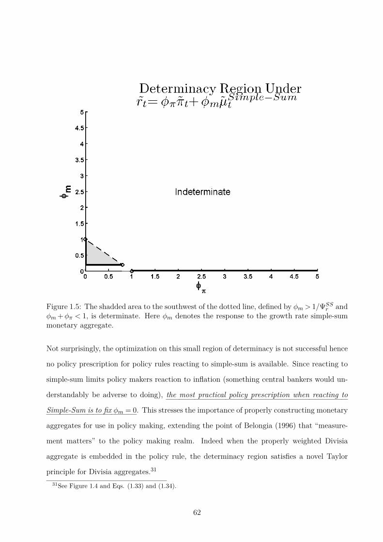
Figure 1.5: The shadded area to the southwest of the dotted line, defined by φm> 1/ΨSSr and

φm+φπ < 1, is determinate. Here φm denotes the response to the growth rate simple-summonetary aggregate.

Not surprisingly, the optimization on this small region of determinacy is not successful hence

no policy prescription for policy rules reacting to simple-sum is available. Since reacting to

simple-sum limits policy makers reaction to inflation (something central bankers would un-

derstandably be adverse to doing), the most practical policy prescription when reacting to

Simple-Sum is to fix φm = 0. This stresses the importance of properly constructing monetary

aggregates for use in policy making, extending the point of Belongia (1996) that “measure-

ment matters” to the policy making realm. Indeed when the properly weighted Divisia

aggregate is embedded in the policy rule, the determinacy region satisfies a novel Taylor

principle for Divisia aggregates.31

31See Figure 1.4 and Eqs. (1.33) and (1.34).

62

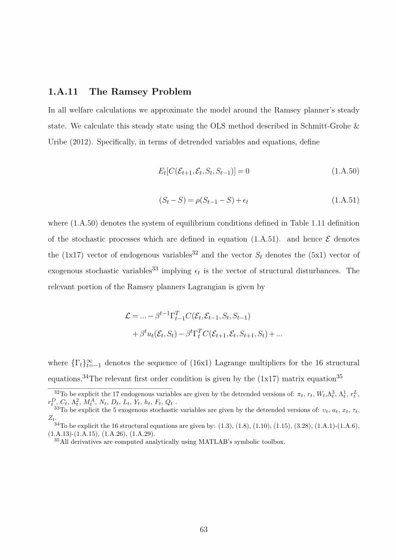
1.A.11 The Ramsey Problem

In all welfare calculations we approximate the model around the Ramsey planner’s steady

state. We calculate this steady state using the OLS method described in Schmitt-Grohe &

Uribe (2012). Specifically, in terms of detrended variables and equations, define

Et[C(Et+1,Et,St,St−1)] = 0 (1.A.50)

(St−S) = ρ(St−1 −S)+ ǫt (1.A.51)

where (1.A.50) denotes the system of equilibrium conditions defined in Table 1.11 definition

of the stochastic processes which are defined in equation (1.A.51). and hence E denotes

the (1x17) vector of endogenous variables32 and the vector St denotes the (5x1) vector of

exogenous stochastic variables33 implying ǫt is the vector of structural disturbances. The

relevant portion of the Ramsey planners Lagrangian is given by

L = ...−βt−1ΓTt−1C(Et,Et−1,St,St−1)

+βtut(Et,St)−βtΓTt C(Et+1,Et,St+1,St)+ ...

where Γt∞t=−1 denotes the sequence of (16x1) Lagrange multipliers for the 16 structural

equations.34The relevant first order condition is given by the (1x17) matrix equation35

32To be explicit the 17 endogenous variables are given by the detrended versions of: πt, rt, Wt,Λ3t , Λ1

t , rLt ,

rDt , Ct, Λ2

t , MAt , Nt, Dt, Lt, Yt, ht, Ft, Qt .

33To be explicit the 5 exogenous stochastic variables are given by the detrended versions of: υt, at, xt, τt,Zt.

34To be explicit the 16 structural equations are given by: (1.3), (1.8), (1.10), (1.15), (3.28), (1.A.1)-(1.A.6),(1.A.13)-(1.A.15), (1.A.26), (1.A.29).

35All derivatives are computed analytically using MATLAB’s symbolic toolbox.

63

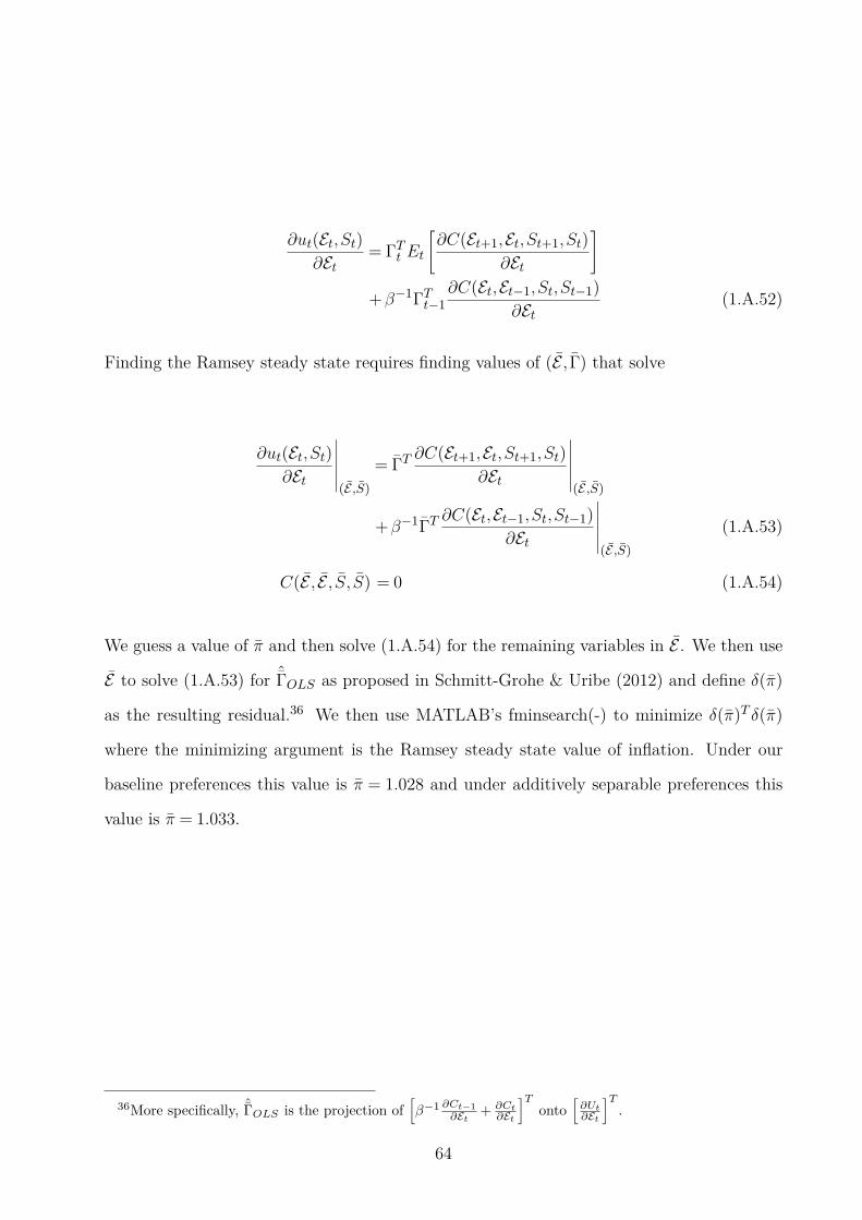
∂ut(Et,St)∂Et

= ΓTt Et

[

∂C(Et+1,Et,St+1,St)

∂Et

]

+β−1ΓTt−1∂C(Et,Et−1,St,St−1)

∂Et(1.A.52)

Finding the Ramsey steady state requires finding values of (E , Γ) that solve

∂ut(Et,St)∂Et

∣∣∣∣∣∣(E ,S)

= ΓT∂C(Et+1,Et,St+1,St)

∂Et

∣∣∣∣∣∣(E ,S)

+β−1ΓT∂C(Et,Et−1,St,St−1)

∂Et

∣∣∣∣∣∣(E ,S)

(1.A.53)

C(E , E , S, S) = 0 (1.A.54)

We guess a value of π and then solve (1.A.54) for the remaining variables in E . We then use

E to solve (1.A.53) for ˆΓOLS as proposed in Schmitt-Grohe & Uribe (2012) and define δ(π)

as the resulting residual.36 We then use MATLAB’s fminsearch(-) to minimize δ(π)T δ(π)

where the minimizing argument is the Ramsey steady state value of inflation. Under our

baseline preferences this value is π = 1.028 and under additively separable preferences this

value is π = 1.033.

36More specifically, ˆΓOLS is the projection of[

β−1 ∂Ct−1

∂Et+ ∂Ct

∂Et

]T

onto[

∂Ut∂Et

]T

.

64

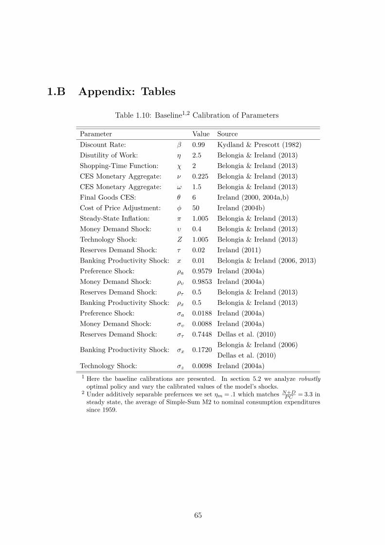
1.B Appendix: Tables

Table 1.10: Baseline1,2 Calibration of Parameters

Parameter Value Source

Discount Rate: β 0.99 Kydland & Prescott (1982)

Disutility of Work: η 2.5 Belongia & Ireland (2013)

Shopping-Time Function: χ 2 Belongia & Ireland (2013)

CES Monetary Aggregate: ν 0.225 Belongia & Ireland (2013)

CES Monetary Aggregate: ω 1.5 Belongia & Ireland (2013)

Final Goods CES: θ 6 Ireland (2000, 2004a,b)

Cost of Price Adjustment: φ 50 Ireland (2004b)

Steady-State Inflation: π 1.005 Belongia & Ireland (2013)

Money Demand Shock: υ 0.4 Belongia & Ireland (2013)

Technology Shock: Z 1.005 Belongia & Ireland (2013)

Reserves Demand Shock: τ 0.02 Ireland (2011)

Banking Productivity Shock: x 0.01 Belongia & Ireland (2006, 2013)

Preference Shock: ρa 0.9579 Ireland (2004a)

Money Demand Shock: ρυ 0.9853 Ireland (2004a)

Reserves Demand Shock: ρτ 0.5 Belongia & Ireland (2013)

Banking Productivity Shock: ρx 0.5 Belongia & Ireland (2013)

Preference Shock: σa 0.0188 Ireland (2004a)

Money Demand Shock: συ 0.0088 Ireland (2004a)

Reserves Demand Shock: στ 0.7448 Dellas et al. (2010)

Banking Productivity Shock: σx 0.1720Belongia & Ireland (2006)

Dellas et al. (2010)

Technology Shock: σz 0.0098 Ireland (2004a)

1 Here the baseline calibrations are presented. In section 5.2 we analyze robustly

optimal policy and vary the calibrated values of the model’s shocks.2 Under additively separable prefernces we set ηm = .1 which matches N+D

P C= 3.3 in

steady state, the average of Simple-Sum M2 to nominal consumption expendituressince 1959.

65

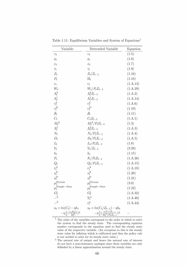
Table 1.11: Equilibrium Variables and System of Equations1

Variable Detrended Variable Equation

υt υt (1.5)

at at (1.6)

xt xt (1.7)

τt τt (1.9)

Zt Zt/Zt−1 (1.16)

Pt Πt (1.18)

rt rt (1.A.13)

Wt Wt/PtZt−1 (1.A.29)

Λ3t Λ3

tZt−1 (1.A.2)

Λ1t Λ1

tZt−1 (1.A.14)

rLt rLt (1.A.6)

rDt rDt (1.10)

St St (1.11)

Ct CtZt−1 (1.A.1)

MAt MA

t /PtZt−1 (1.3)

Λ2t Λ2

tZt−1 (1.A.3)

Nt Nt/PtZt−1 (1.A.4)

Dt Dt/PtZt−1 (1.A.5)

Lt Lt/PtZt−1 (1.8)

Yt Yt/Zt−1 (3.28)

ht ht (1.15)

Ft Ft/PtZt−1 (1.A.26)

Qt Qt/PtZt−1 (1.A.15)

rAt rAt (1.A.18)

sNt sNt (1.20)

sDt sDt (1.21)

µDivisiat µDivisiat (3.8)

µSimple−Sumt µSimple−Sumt (1.22)

Get Get (1.A.32)

−2 Y nt (1.A.40)

−2 rnt (1.A.44)

ut = ln(Ct)−ηht ut = ln(Ct/Zt−1)−ηht

−η 1χ(υtPtCt

MAt

)χ −η 1χ( υtCt/Zt−1

MAt /PtZt−1

)χ −1 The order of the variables correspond to the order in which to solve

the system to find the steady state. The corresponding equationnumber corresponds to the equation used to find the steady statevalue of the respective variable. (An exception to this is the steadystate value for inflation which is calibrated and thus the policy ruleis not needed to solve for its steady state value.)

2 The natural rate of output and hence the natural rate of interestdo not have a non-stationary analogue since these variables are onlydefinded by a linear approximation around the steady state.

66

Chapter 2

Determinacy and Indeterminacy in

Monetary Policy Rules with Money1

2.1 Introduction

In his classic (1960) work, A Program for Monetary Stability, Milton Friedman argued the

economy can be stabilized by stabilizing the growth rate of a money at k-percent. This policy

proposal has received considerable attention by monetary theorist.2 Surprisingly though, the

question of whether this rule could be implemented with a broad monetary aggregate in a

manner which delivers a unique rational expectations equilibrium remains unanswered. If

such a rule fails in this capacity, fixing the growth rate of a monetary aggregate may induce

instability by allowing for sunspot equilibria. This paper provides an answer to this question

within the preferred framework of modern monetary policy analysis, a New-Keynesian model.

We show analytically that Friedman’s k-percent rule can deliver a unique rational expecta-

tions equilibrium when the true monetary aggregate is used. Since that aggregate depends

on deep structural parameters, such a rule is not simple in the sense defined by (Gali, 2008).

1This chapter is coauthored with John W. Keating, Department of Economics, The University of Kansas,Email: jkeating@ku.edu.

2For example, Ireland (1996) has shown that a policy of holding the growth rate of money constant canbe optimal from a welfare perspective when prices are set in advance. Additionally, Carlstrom & Fuerst(1995, 2003) explore the welfare and determinacy properties of money growth rules in flexible price models.

67

A simple rule which could actually be used by central banks,3 would be to fix the growth

rate of the Divisia monetary aggregate. We show that such a rule inherits the determi-

nacy properties of the k-percent rule based on using the true monetary aggregate. Another

well-known non-parametric aggregate is the simple-sum monetary aggregate which was the

method used to compute the M2 measure Friedman advocated. Interestingly, if this aggre-

gate is used in place of the true monetary aggregate,we find Friedman’s k-percent rule is

likely to result in indeterminacy stemming from the simple-sum’s error in tracking the true

aggregate. We conclude that Friedman was correct in his judgment that fixing the growth

rate of a broad monetary aggregate may stabilize the economy. However, we show in the

context of a New-Keynesian model with multiple types of assets which provide monetary

services that aggregation by simple-sum is in general a flawed approach.

Most similar to our work is Evans & Honkapohja (2003). They analyze determinacy prop-

erties of k-percent rules in a New-Keynesian model when money is modeled as a single

monetary asset. In this case, money in the model can be interpreted as base money since

it earns zero interest. They show numerically that fixing the growth rate of this measure of

money is consistent with a unique rational expectations equilibrium under a broad range of

values. However Friedman’s k-percent rule calls for the central bank to fix the growth rate

of a high-level monetary aggregate, not base money. In order to analyze determinacy prop-

erties of broad monetary aggregates, we require a model like the one developed by Belongia

& Ireland (2014) which provides a role for both currency and deposits as competing sources

of monetary services. We use this as our framework to analyze the determinacy properties

of monetary policy rules with broad money.

In addition to providing analytic representations of the determinacy regions of various mon-

etary aggregate growth rules, we also analyze interest rate rules reacting to inflation and the

growth rate of monetary aggregates. Once again we find that "measurement matters” (Belon-

gia, 1996) from a determinacy standpoint. Interest rate rules reacting to the growth rate of

3Arguably, one reason Friedman advocated a k-percent rule was its simplicity.

68

either the true monetary aggregate or the Divisia monetary aggregate satisfy a novel Taylor

principle for monetary aggregates. The simple-sum monetary aggregate’s error in tracking

the true aggregate prevents an interest rate rule reacting to simple-sum from having a similar

determinacy region. Instead, such rules have very small determinacy regions.

Following this introductory section we present our model which is a standard New-Keynesian

framework that allows two different types of assets to provide monetary services. Section 3

examines determinacy properties of k-percent rules and compares outcomes obtained with

different monetary aggregates. The fourth section of the paper investigates interest rate rules

that allow for a reaction to monetary aggregates. Again we address determinacy properties

associated with alternative monetary aggregates. Section 5 performs a numerical analysis

with more complicated monetary policy rules that allow policy to react to more information

making it impossible to derive analytical results. Section 6 concludes the paper.

2.2 Model

We consider a canonical version of the linearized New-Keynesian (NK) model. Following

Woodford’s (2003) notation we assume all exogenous disturbances are bounded in amplitude

by ‖ξ‖. All variables with a "–" over them denote non-stochastic steady-state values. Also,

variables with a "~" over them denote log-deviations from the non-stochastic steady state. For

convenience of notation we assume each stochastic disturbance follows a stationary AR(1)

process and is driven by orthogonal white noise shocks. However, this assumption is only

made for convenience as all the results presented hold for general stationary processes. As

usual, this model consists of 3 non-policy equations when money is included in the model.

yet = Etyet+1− [rt−Etπt+1− ret ] (2.1)

πt = κyet +βEtπt+1 (2.2)

mt− pt = yet − ut+ υt+ zt (2.3)

69

Equation (2.1) is the dynamic IS curve, equation (2.2) is the New-Keynesian Phillips Curve

(NKPC) and equation (2.3) is the demand for the monetary aggregate. In the above equa-

tions yet = yt − zt denotes the efficient output gap and ret = Et∆zt+1 −Etat+1 denotes

the efficient interest rate. The variables zt, at, and υt represent exogenous technology, pref-

erence and money-demand disturbances respectively. We depart from the textbook analysis

of money. Following Belongia & Ireland (2014) we model broad money so that (2.3) is the

demand for the aggregate service flow from currency and interest bearing deposits. For this

reason, (2.3) includes the user-cost of the monetary aggregate ut which in general depends

on a vector of interest rates. Modeling money as a broader measure turns out to play a key

role in our determinacy results. In addition to examining the effects of monetary aggregate

growth rules we will also investigate interest rate rules which react to the growth rate of a

monetary aggregate.

We assume a constant elasticity of substitution (CES) function:

mt =[

ν1ωn

ω−1ω

t +(1−ν)1ω d

ω−1ω

t

] ωω−1

(2.4)

is the true monetary aggregate where nt and dt are non interest bearing currency and interest

bearing deposits respectively. Meanwhile, ω > 0 is the elasticity of substitution between

currency and deposits and 0< ν < 1 governs the steady-state share of currency and deposits.

The CES function is homogeneous of degree one in terms of nt and dt, an attractive property

since that means changing both nt and dt by a certain percentage will change the monetary

aggregate by exactly that same percentage. Of course, simple-sum has that property. And

when ω → ∞, mt = nt+ dt. Hence, the simple-sum monetary aggregate is the appropriate

monetary aggregate when currency and deposits are perfect substitutes. More generally,

when ω <∞, currency and deposits are not perfect one-for-one substitutes and then simple-

sum will not equal the true aggregate.

70

The aggregate dual user-cost is correspondingly defined by

ut =

ν(rt−1

rt

)1−ω

+(1−ν)

(

rt− rdtrt

)1−ω

11−ω

. (2.5)

Following the structural model of Belongia & Ireland (2014) with profit maximizing banks,

the user cost of deposits can be expressed as

udt =rt− rdtrt

=(rt−1)τt+xt

rt(2.6)

where rt is the gross nominal interest rate on loans, rdt is the deposit rate and both τt

and xt are exogenous financial disturbances that follow stationary stochastic processes with

orthogonal white noise shocks. Specifically, τt represents reserves demand disturbances with

a mean τ and xt represents deposit cost disturbances with a mean x. To remain empirically

relevant, we will assume throughout the paper that the stochastic processes are bounded so

that at all times rt > rdt > 1 ensuring that deposits are “cheaper” than currency. A log-linear

approximation to (2.5) is given by

ut = ηrrt+ητ τt+ηxxt+O(‖ξ‖2) (2.7)

where all the coefficients are positive. Substituting (2.7) into (2.3) brings about a five variable

dynamic model with three equations (2.1, 2.2 and 2.8).

mt− pt = yet −ηrrt−ητ τt−ηxxt+ υt+ zt (2.8)

The dimension of the model can be reduced by one variable after defining real balances as

lt ≡ mt− pt. As is standard, we close the model with a specification of monetary policy.

71

2.3 Friedman k-percent Rules

In this section we consider the performance of various money growth rules. Initially we close

the model with a constant money growth rule for the true monetary aggregate:

∆mt = 0. (2.1)

Such k-percent rules have been examined in New-Keynesian models by Evans & Honkapohja

(2003) and Gali (2008) where they were shown to deliver a unique REE. However, these

studies assume the existence of a single monetary asset. This leaves open the question

of whether the determinacy properties extend to measures that aggregate different types

of monetary assets. Arguably, this is the relevant case to consider. Friedman, for example,

argued for fixing the growth rate of a broad aggregate such as M2, not the monetary base. In

this section we show three main results. First, the k-percent rule is always determinate when

applied to the true monetary aggregate, regardless of the magnitude of the interest semi-

elasticity. Second, this result of general determinacy extends to rules in the true aggregate

is replaced by the Divisia monetary aggregate. Finally, we show that this strong result does

not extend to the simple-sum monetary aggregate. Instead, a constant simple-sum growth

rule is indeterminate unless the interest semi-elasticity is large relative to simple-sum’s error

in tracking the true monetary aggregate. Consider the dynamic system consisting of (2.1),

(2.2), (2.8) and (2.1).

Proposition 2.1. For any 0 < β < 1, for any κ > 0 and for any ηr ≥ 0 if the central bank

follows the policy rule ∆mt = 0 then there exists a unique REE.

The proof of this proposition is in the Appendix. Unless stated otherwise, the proof for the

remaining propositions, lemma and corollaries will also be found in the Appendix. Proposi-

tion 1 shows that a constant monetary aggregate growth rules always deliver a unique REE

provided it is based on the true monetary aggregate. This result extends results of Evans &

72

Honkapohja (2003) to monetary aggregates. This result in of itself is of little use to central

banks who do not know the underlying parameters of the monetary aggregate. To circum-

vent this problem, suppose the central bank fixes the growth rate of the Divisia monetary

aggregate instead of the true monetary aggregate developed initially by Barnett (1980).

Definition 2.1. The growth rate of the Divisia monetary aggregate is defined by:

ln(gdivisiat ) =

(

snt + snt−1

2

)

ln

(

ntnt−1

)

+

(

sdt + sdt−1

2

)

ln

(

dtdt−1

)

, (2.2)

where snt and sdt are the expenditure shares of currency and interest bearing deposits respec-

tively defined by:

snt =(rt−1)nt

(rt−1)nt+(rt− rdt )dtand sdt = 1− snt . (2.3)

The Divisia monetary aggregate is the expenditure share-weighed growth rate of currency

and deposits. In contrast to the true aggregate, the Divisia aggregate is non-parametric and

depends only on current and past observable information. Such a rule is more relevant to

policy makers as it doesn’t require estimating any parameters.4

The following lemma shows that for the general CES specification ofmt, the Divisia monetary

aggregate (locally) tracks the growth rate of the true monetary aggregate to first order

accuracy without error.

Lemma 2.1. For any 0 < ν < 1 and for any ω > 0, the difference between the Divisia

monetary aggregate and the true monetary is given by

ln(gdivisiat )−∆ln(Mt) = O(‖ξ‖2).

The accuracy properties of the Divisia monetary aggregate are well known in Index number

4A central bank could estimate the parameters in equation 4, the monetary aggregator function, but thatwould induce parameter uncertainty from sampling error, but using Divisia avoids that concern. Moreover,this approach leaves a central bank exposed to questions and criticisms with regards to how they estimatethe parameters.

73

theory. Most notably, Divisia (1926) showed in continuous time, the Divisia monetary ag-

gregate tracks any linearly homogenous function without error. Moreover, Diewert (1976)

classified the discrete time Divisia monetary aggregate defined above as superlative - mean-

ing that it can track the growth rate of any twice differentiable linearly homogenous function

up to second order accuracy without error. This lemma shows that for the CES function in

particular, a linear approximation to the Divisia monetary aggregate tracks the true mone-

tary aggregate up to first order accuracy without error. This result is very useful in analyzing

local determinacy which requires only a linear approximation to the non-linear model.

Formally, suppose the central bank follows the rule

gdivisiat = 0 (2.4)

in place of (2.1). The dynamic system consists of (2.1), (2.2), (2.8) and (2.4), and we obtain

the following result.

Corollary 2.1. For any 0 < β < 1, for any κ > 0 and for any ηr ≥ 0 if the central bank

follows the policy rule gdivisiat = 0 then there exists a unique REE.

The proof follows immediately from combining Lemma 1 and Proposition 1. Corollary 1

shows the central bank may replace the true aggregate with the Divisia monetary aggregate

without any change in determinacy. This result obtains because determinacy is a local

condition and Lemma 1 shows that locally, the Divisia monetary aggregate exactly tracks

the growth rate of the true monetary aggregate. Therefore, determinacy properties for

growth rules based on the true monetary aggregate are inherited by rules which instead use

the Divisia monetary aggregate. However, the same can not be said for the more common

simple-sum monetary aggregate.

Definition 2.2. The growth rate of the simple-sum monetary aggregate is defined by

ln(gsimple−sumt ) = ln

(

nt+dtnt−1 +dt−1

)

. (2.5)

74

The simple-sum aggregate treats currency and interest bearing deposits as one for one per-

fect substitutes. Standard microeconomic theory dictates in such a case only the cheapest

monetary asset would have a positive demand in equilibrium. Since this is not the case in

this model, nor reality, it is perhaps not surprising the simple-sum aggregate will locally

track the true aggregate with error. The following lemma defines and quantifies this error.

Lemma 2.2. For any 0 < ν < 1, for any ω > 0 and for any (τ , x) satisfying (r− 1) >

(r− 1)τ +x so that un > ud > 0, the difference between the growth rate of the simple-sum

monetary aggregate and the growth rate of the true monetary aggregate is given by

ln(gsimple−sumt )−∆ln(mt) = ψr(ω)∆rt−ψx(ω)∆xt−ψτ (ω)∆τt+O(‖ξ‖2) (2.6)

where

(

ψr(ω), ψx(ω), ψτ (ω)

)

∈ R3++ with lim

ω→∞ψr(ω) = ψx(ω) = ψτ (ω) = 0.

Intuitively, any change in the relative prices of currency and deposits results in a substitution

between these assets from the household. Since the simple-sum monetary aggregate treats

these assets as perfect one for one substitutes it is not able to internalize these relative

changes in the service flow from the monetary aggregate. Only in the limiting case of perfect

substitutes does this error disappear.

From a determinacy standpoint, simple-sum’s error in tracking the true monetary aggregate

arising from the exogenous financial shocks is irrelevant. However, the error that depends

on the endogenous interest rate - ∆rt - will influence the determinacy region of a rule uti-

lizing the simple-sum monetary aggregate. In particular, the following corollary summarizes

determinacy properties when instead of (2.1) the policy rule is:

gsimple−sumt = 0, (2.7)

with the dynamic system now consisting of (2.1), (2.2), (2.8) and (2.7).

75

Corollary 2.2. For any 0 < β < 1, for any κ > 0 if the central bank follows the policy rule

gsimple−sumt = 0 then there exists a unique REE if and only if ψr(ω)< ηr + 12 .

Importantly, when using the simple-sum monetary aggregate in place of either the true mon-

etary aggregate or the Divisia monetary aggregate a constant monetary aggregate growth

rule may not be determinate. Indeterminacy will occur when the error term ψr(ω) is large

relative to the interest semi-elasticity of money demand - ηr. This parameter varies signifi-

cantly in the empirical literature. For example Ball (2001) estimates ηr = .05 while Ireland

(2009) estimates ηr = 1.9. Given the wide range of estimates for ηr, central banks may be un-

derstandably averse to implementing this Friedman’s k-percent rule based on a simple-sum

measure. Furthermore, Section 2.5 of this paper presents estimates of ψr(ω) which com-

bined with even the largest plausible estimates of ηr suggest that the determinacy condition

in Corollary 2 is unlikely to be satisfied. On the other hand, a k-percent rule with Divisia

yields no determinacy concerns whatsoever.

2.4 Interest Rate Rules with Money

In this section we consider interest rate feedback rules which react to lagged interest rates and

the growth rate of a monetary aggregate. When Friedman proposed the k-percent rule, he

also advocated changes in bank regulation which would make the rule easily implemented.

For example, Friedman (1960) argued for increasing the reserve requirements to 100% to

make the monetary aggregates more easily controllable. Friedman (1960) went on to say

that:

This [constant money growth] is not, under our present System, an easy thing

to do. It involves a great many technical difficulties and there will be some

deviations from it. If the other changes I suggested were made in the System,

it would make the task easier; but even without those changes, it could be done

under the present System.

76

Under a fractional reserve banking system a pragmatic way of targeting the growth rate of

money is with an interest rate reaction function whereby the central bank adjusts the interest

rate as needed to correct deviations of money growth from the desired k-percent target.

More recently a number of studies have included nominal money growth in interest rate

rules such as Canova & Menz (2011), Sims & Zha (2006) and Fahr et al. (2013). Fewer

papers have included Divisia monetary aggregates in interest rate feedback rules. One that

has is Belongia & Ireland (2012) which estimates structural VAR’s with such rules. Keating

& Smith (2013) find that interest rate rules that react to Divisia may be optimal from

a normative perspective if financial shocks are present and the natural rate of interest is

unobservable. This result is consistent with the assertion of McCallum & Nelson (2011) and

Andres et al. (2009) that nominal money growth provides valuable real-time information

regarding the natural rate of interest. Despite this interest, there are no results on the

determinacy properties of such rules to guide policy makers. With this in mind, assume the

central bank sets the policy rate according to

rt = φrrt−1 +φm∆mt. (2.1)

Using (2.1) to close the dynamic model that still contains (2.1), (2.2) and (2.8), we have the

following result.

Proposition 2.2. For any 0 < β < 1, for any κ > 0 and for any ηr ≥ 0, if the central bank

follows the policy rule rt = φrrt−1 +φm∆mt with φm ≥ 0 and φr ≥ 0 then there exists a unique

REE if and only if φm+φr > 1.

Intuitively, this result extends the Taylor Principle to monetary aggregates. Expectations will

remain well-anchored if the central bank reacts more than one for one to nominal aggregate-

money growth, in the long-run. Proposition 1 provides a sufficient condition for determinacy

that is independent of the magnitude of the interest semi-elasticity of money demand which

is important given that the estimates of this parameter vary significantly in the empirical

77

literature.

Despite the neutrality of the result with regard to ηr, this rule requires that a central bank

measure the unobservable true monetary aggregate. To circumvent this issue suppose instead

the central bank replaces the true monetary aggregate with the Divisia monetary aggregate

rt = φrrt−1 +φdgdivisiat . (2.2)

The policy rule in (2.2) could more be easily implemented by a central bank compared to

(2.1) as the interest rate is responding to observable information and does not entail the

estimation of any deep structural parameters. Ans the following corollary to Proposition 2

shows that a central bank can replace ∆m with gdivisiat without changing the determinacy

condition.

Corollary 2.3. For any 0 < β < 1, for any κ > 0 and for any ηr ≥ 0 if the central bank

follows the policy rule rt = φrrt−1 +φdgdivisiat with φd ≥ 0 and φr ≥ 0 then there exists a

unique REE if and only if φd+φr > 1.

The proof of this corollary follows immediately by combining Lemma 1 with Proposition 2.

This result is significant in terms of actually implementing interest rate rules reacting to

money growth. Most notably, central banks can use the non-parametric Divisia aggregate

in interest rate feedback rules like (2.2) and guarantee determinacy by setting φd > 1.

The same can not be said, however, for the more common simple-sum monetary aggregate.

In particular, the following corollary summarizes determinacy properties when the policy

rule in (2.3) is used instead of (2.1) or (2.2)

rt = φrrt−1 +φssgsimple−sum. (2.3)

Corollary 2.4. For any 0 < β < 1, for any κ > 0 and for any ηr ≥ 0 if the central bank

follows the policy rule rt = φrrt−1 +φssgsimple−sum with φss ≥ 0 and φr ≥ 0 then there exists

78

a unique REE if and only if | φr +φss−φss[ψr(ω)−ηr] |>| 1−φss[ψr(ω)−ηr] |.

A proof of this derives from Lemma 2 and Proposition 2 and is found in the Appendix.

This result highlights how once again simple-sum and Divisia monetary aggregates diverge

in terms of determinacy properties. Namely, the determinacy region for interest rate rules

reacting to the simple-sum monetary aggregate depend on simple-sum’s error in tracking the

true monetary aggregate. Intuitively, if ψr(ω) is relatively large compared to the interest

semi-elasticity of money demand then an upper and lower bound is placed on φss for de-

terminacy. Meanwhile, if ψr(ω) is relatively small compared to the interest semi-elasticity

of money demand then only a lower bound is placed on φss for determinacy. For example,

in the extreme case where the simple-sum and Divisia aggregates coincide (i.e. ω → ∞),

Corollary 3 shows that φss > 1 is sufficient for determinacy. However, in the more general

case, determinacy under the interest rate rule reacting to simple-sum may have a relatively

small determinacy region as summarized below for the case in which ψr(ω) − ηr > 1. The

following section of the paper provides an empirical justification for assuming this inequality

holds.

To get an idea of how likely determinacy is under an interest rate rule reacting to the

simple-sum aggregate Figure 1 plots the determinacy region under the numerical calibration

presented below. There are 2 regions of determinacy. Using Leeper’s (1991) terminology, one

region is in the passive regime while the other is in the active regime. What stands out the

most is how unlikely the condition presented in Corollary 4 is satisfied. Under this interest

rate rule with simple-sum money determinacy occurs within such a narrow band that it is

more the exception than the norm.

2.5 Numerical Analysis

Potentially more realistic policy rules may include not only a response to the growth rate

of a monetary aggregate but also a response to inflation. Unfortunately this slightly more

complicated rule places analytic results out of reach so we must resort to numerical anal-

79

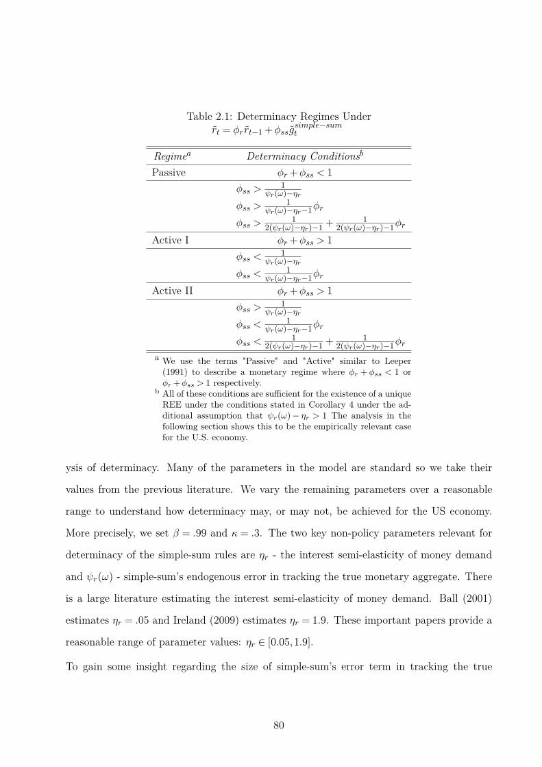
Table 2.1: Determinacy Regimes Underrt = φrrt−1 +φssg

simple−sumt

Regimea Determinacy Conditionsb

Passive φr +φss < 1

φss >1

ψr(ω)−ηr

φss >1

ψr(ω)−ηr−1φr

φss >1

2(ψr(ω)−ηr)−1 + 12(ψr(ω)−ηr)−1φr

Active I φr +φss > 1

φss <1

ψr(ω)−ηr

φss <1

ψr(ω)−ηr−1φr

Active II φr +φss > 1

φss >1

ψr(ω)−ηr

φss <1

ψr(ω)−ηr−1φr

φss <1

2(ψr(ω)−ηr)−1 + 12(ψr(ω)−ηr)−1φr

a We use the terms "Passive" and "Active" similar to Leeper(1991) to describe a monetary regime where φr + φss < 1 orφr +φss > 1 respectively.

b All of these conditions are sufficient for the existence of a uniqueREE under the conditions stated in Corollary 4 under the ad-ditional assumption that ψr(ω) − ηr > 1 The analysis in thefollowing section shows this to be the empirically relevant casefor the U.S. economy.

ysis of determinacy. Many of the parameters in the model are standard so we take their

values from the previous literature. We vary the remaining parameters over a reasonable

range to understand how determinacy may, or may not, be achieved for the US economy.

More precisely, we set β = .99 and κ = .3. The two key non-policy parameters relevant for

determinacy of the simple-sum rules are ηr - the interest semi-elasticity of money demand

and ψr(ω) - simple-sum’s endogenous error in tracking the true monetary aggregate. There

is a large literature estimating the interest semi-elasticity of money demand. Ball (2001)

estimates ηr = .05 and Ireland (2009) estimates ηr = 1.9. These important papers provide a

reasonable range of parameter values: ηr ∈ [0.05,1.9].

To gain some insight regarding the size of simple-sum’s error term in tracking the true

80

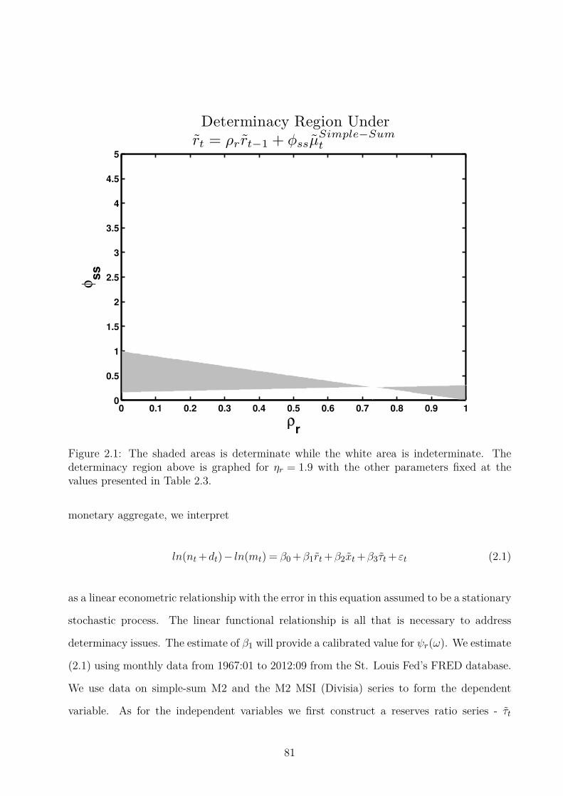
0 0.1 0.2 0.3 0.4 0.5 0.6 0.7 0.8 0.9 10

0.5

1

1.5

2

2.5

3

3.5

4

4.5

5

ρr

φ ss

Determinacy Region Underrt = ρr rt−1 + φssµ

Simple−Sumt

Figure 2.1: The shaded areas is determinate while the white area is indeterminate. Thedeterminacy region above is graphed for ηr = 1.9 with the other parameters fixed at thevalues presented in Table 2.3.

monetary aggregate, we interpret

ln(nt+dt)− ln(mt) = β0 +β1rt+β2xt+β3τt+ εt (2.1)

as a linear econometric relationship with the error in this equation assumed to be a stationary

stochastic process. The linear functional relationship is all that is necessary to address

determinacy issues. The estimate of β1 will provide a calibrated value for ψr(ω). We estimate

(2.1) using monthly data from 1967:01 to 2012:09 from the St. Louis Fed’s FRED database.

We use data on simple-sum M2 and the M2 MSI (Divisia) series to form the dependent

variable. As for the independent variables we first construct a reserves ratio series - τt

81

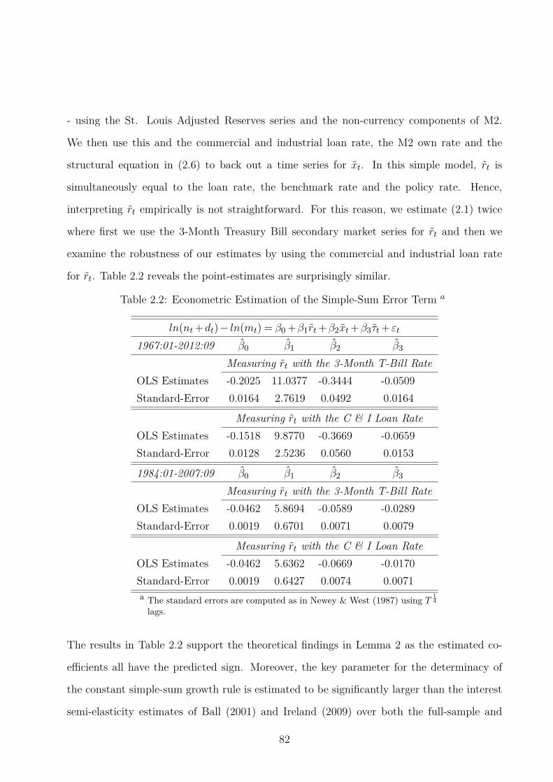
- using the St. Louis Adjusted Reserves series and the non-currency components of M2.

We then use this and the commercial and industrial loan rate, the M2 own rate and the

structural equation in (2.6) to back out a time series for xt. In this simple model, rt is

simultaneously equal to the loan rate, the benchmark rate and the policy rate. Hence,

interpreting rt empirically is not straightforward. For this reason, we estimate (2.1) twice

where first we use the 3-Month Treasury Bill secondary market series for rt and then we

examine the robustness of our estimates by using the commercial and industrial loan rate

for rt. Table 2.2 reveals the point-estimates are surprisingly similar.

Table 2.2: Econometric Estimation of the Simple-Sum Error Term a

ln(nt+dt)− ln(mt) = β0 +β1rt+β2xt+β3τt+ εt

1967:01-2012:09 β0 β1 β2 β3

Measuring rt with the 3-Month T-Bill Rate

OLS Estimates -0.2025 11.0377 -0.3444 -0.0509

Standard-Error 0.0164 2.7619 0.0492 0.0164

Measuring rt with the C & I Loan Rate

OLS Estimates -0.1518 9.8770 -0.3669 -0.0659

Standard-Error 0.0128 2.5236 0.0560 0.0153

1984:01-2007:09 β0 β1 β2 β3

Measuring rt with the 3-Month T-Bill Rate

OLS Estimates -0.0462 5.8694 -0.0589 -0.0289

Standard-Error 0.0019 0.6701 0.0071 0.0079

Measuring rt with the C & I Loan Rate

OLS Estimates -0.0462 5.6362 -0.0669 -0.0170

Standard-Error 0.0019 0.6427 0.0074 0.0071

a The standard errors are computed as in Newey & West (1987) using T14

lags.

The results in Table 2.2 support the theoretical findings in Lemma 2 as the estimated co-

efficients all have the predicted sign. Moreover, the key parameter for the determinacy of

the constant simple-sum growth rule is estimated to be significantly larger than the interest

semi-elasticity estimates of Ball (2001) and Ireland (2009) over both the full-sample and

82

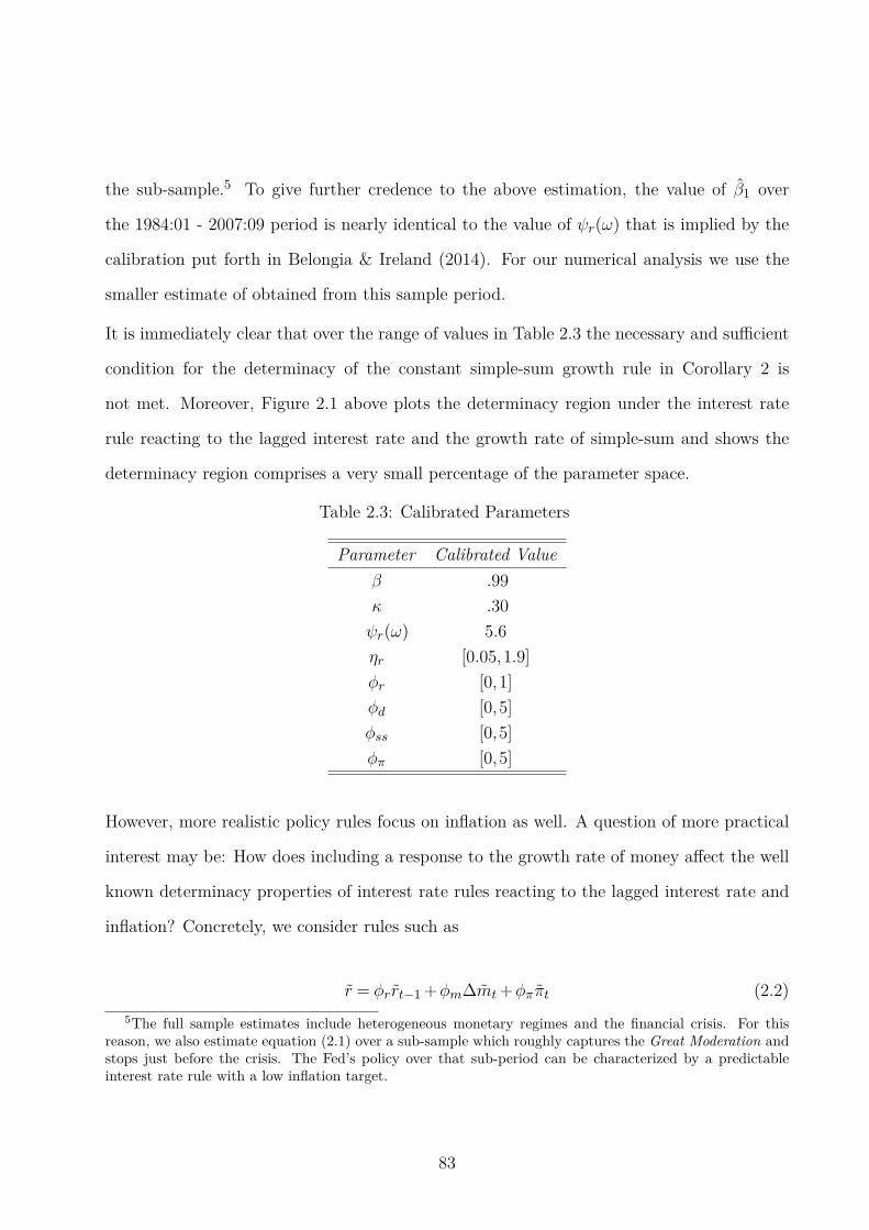
the sub-sample.5 To give further credence to the above estimation, the value of β1 over

the 1984:01 - 2007:09 period is nearly identical to the value of ψr(ω) that is implied by the

calibration put forth in Belongia & Ireland (2014). For our numerical analysis we use the

smaller estimate of obtained from this sample period.

It is immediately clear that over the range of values in Table 2.3 the necessary and sufficient

condition for the determinacy of the constant simple-sum growth rule in Corollary 2 is

not met. Moreover, Figure 2.1 above plots the determinacy region under the interest rate

rule reacting to the lagged interest rate and the growth rate of simple-sum and shows the

determinacy region comprises a very small percentage of the parameter space.

Table 2.3: Calibrated Parameters

Parameter Calibrated Value

β .99

κ .30

ψr(ω) 5.6

ηr [0.05,1.9]

φr [0,1]

φd [0,5]

φss [0,5]

φπ [0,5]

However, more realistic policy rules focus on inflation as well. A question of more practical

interest may be: How does including a response to the growth rate of money affect the well

known determinacy properties of interest rate rules reacting to the lagged interest rate and

inflation? Concretely, we consider rules such as

r = φrrt−1 +φm∆mt+φππt (2.2)

5The full sample estimates include heterogeneous monetary regimes and the financial crisis. For thisreason, we also estimate equation (2.1) over a sub-sample which roughly captures the Great Moderation andstops just before the crisis. The Fed’s policy over that sub-period can be characterized by a predictableinterest rate rule with a low inflation target.

83

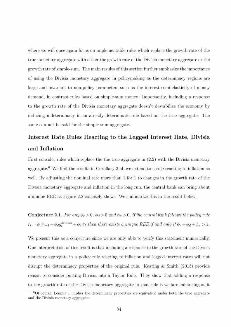
where we will once again focus on implementable rules which replace the growth rate of the

true monetary aggregate with either the growth rate of the Divisia monetary aggregate or the

growth rate of simple-sum. The main results of this section further emphasize the importance

of using the Divisia monetary aggregate in policymaking as the determinacy regions are

large and invariant to non-policy parameters such as the interest semi-elasticity of money

demand, in contrast rules based on simple-sum money. Importantly, including a response

to the growth rate of the Divisia monetary aggregate doesn’t destabilize the economy by

inducing indeterminacy in an already determinate rule based on the true aggregate. The

same can not be said for the simple-sum aggregate.

Interest Rate Rules Reacting to the Lagged Interest Rate, Divisia

and Inflation

First consider rules which replace the the true aggregate in (2.2) with the Divisia monetary

aggregate.6 We find the results in Corollary 3 above extend to a rule reacting to inflation as

well. By adjusting the nominal rate more than 1 for 1 to changes in the growth rate of the

Divisia monetary aggregate and inflation in the long run, the central bank can bring about

a unique REE as Figure 2.2 concisely shows. We summarize this in the result below.

Conjecture 2.1. For any φr > 0, φd> 0 and φπ > 0, if the central bank follows the policy rule

rt = φrrt−1 +φdgdivisiat +φππt then there exists a unique REE if and only if φr+φd+φπ > 1.

We present this as a conjecture since we are only able to verify this statement numerically.

One interpretation of this result is that including a response to the growth rate of the Divisia

monetary aggregate in a policy rule reacting to inflation and lagged interest rates will not

disrupt the determinacy properties of the original rule. Keating & Smith (2013) provide

reason to consider putting Divisia into a Taylor Rule. They show that adding a response

to the growth rate of the Divisia monetary aggregate in that rule is welfare enhancing as it

6Of course, Lemma 1 implies the determinacy properties are equivalent under both the true aggregateand the Divisia monetary aggregate.

84

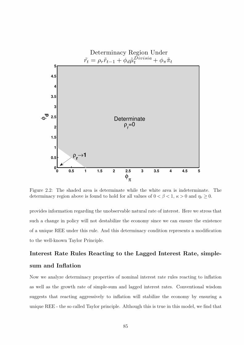
0 0.5 1 1.5 2 2.5 3 3.5 4 4.5 50

0.5

1

1.5

2

2.5

3

3.5

4

4.5

5

φπ

φ d

Determinacy Region Underrt = ρr rt−1 + φdµ

Divisiat + φππt

ρr→1

Determinateρ

r=0

Figure 2.2: The shaded area is determinate while the white area is indeterminate. Thedeterminacy region above is found to hold for all values of 0< β < 1, κ > 0 and ηr ≥ 0.

provides information regarding the unobservable natural rate of interest. Here we stress that

such a change in policy will not destabilize the economy since we can ensure the existence

of a unique REE under this rule. And this determinacy condition represents a modification

to the well-known Taylor Principle.

Interest Rate Rules Reacting to the Lagged Interest Rate, simple-

sum and Inflation

Now we analyze determinacy properties of nominal interest rate rules reacting to inflation

as well as the growth rate of simple-sum and lagged interest rates. Conventional wisdom

suggests that reacting aggressively to inflation will stabilize the economy by ensuring a

unique REE - the so called Taylor principle. Although this is true in this model, we find that

85

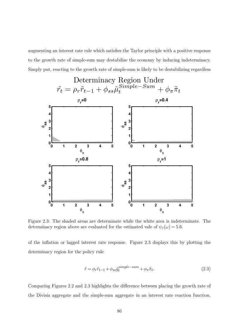
augmenting an interest rate rule which satisfies the Taylor principle with a positive response

to the growth rate of simple-sum may destabilize the economy by inducing indeterminacy.

Simply put, reacting to the growth rate of simple-sum is likely to be destabilizing regardless

0 1 2 3 4 50

1

2

3

4

5

φπ

φ ss

ρr=0

0 1 2 3 4 50

1

2

3

4

5

φπ

φ ss

ρr=0.4

0 1 2 3 4 50

1

2

3

4

5

φπ

φ ss

ρr=0.8

Determinacy Region Underrt = ρr rt−1 + φssµ

Simple−Sumt + φππt

0 1 2 3 4 50

1

2

3

4

5

φπ

φ ss

ρr=1

Figure 2.3: The shaded areas are determinate while the white area is indeterminate. Thedeterminacy region above are evaluated for the estimated vale of ψr(ω) = 5.6.

of the inflation or lagged interest rate response. Figure 2.3 displays this by plotting the

determinacy region for the policy rule

r = φrrt−1 +φssgsimple−sumt +φππt. (2.3)

Comparing Figures 2.2 and 2.3 highlights the difference between placing the growth rate of

the Divisia aggregate and the simple-sum aggregate in an interest rate reaction function.

86

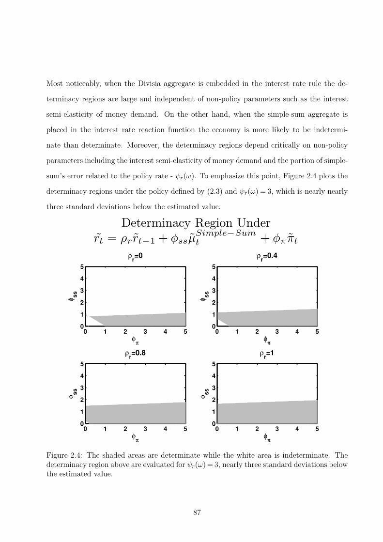
Most noticeably, when the Divisia aggregate is embedded in the interest rate rule the de-

terminacy regions are large and independent of non-policy parameters such as the interest

semi-elasticity of money demand. On the other hand, when the simple-sum aggregate is

placed in the interest rate reaction function the economy is more likely to be indetermi-

nate than determinate. Moreover, the determinacy regions depend critically on non-policy

parameters including the interest semi-elasticity of money demand and the portion of simple-

sum’s error related to the policy rate - ψr(ω). To emphasize this point, Figure 2.4 plots the

determinacy regions under the policy defined by (2.3) and ψr(ω) = 3, which is nearly nearly

three standard deviations below the estimated value.

0 1 2 3 4 50

1

2

3

4

5

φπ

φ ss

ρr=0

0 1 2 3 4 50

1

2

3

4

5

φπ

φ ss

ρr=0.4

0 1 2 3 4 50

1

2

3

4

5

φπ

φ ss

ρr=0.8

Determinacy Region Underrt = ρr rt−1 + φssµ

Simple−Sumt + φππt

0 1 2 3 4 50

1

2

3

4

5

φπ

φ ss

ρr=1

Figure 2.4: The shaded areas are determinate while the white area is indeterminate. Thedeterminacy region above are evaluated for ψr(ω) = 3, nearly three standard deviations belowthe estimated value.

87

Figure 2.4 highlights how sensitive the determinacy regions are to this parameter. Very simi-

lar results are found if we again set ψr(ω) = 5.6 and analyze determinacy under a much larger

value of ηr = 3.8, twice the estimated value from Ireland (2009). This suggests what matters

most for the determinacy properties of simple-sum oriented policy rules is not the policy pa-

rameters, but the size of that aggregate’s error ψr(ω) relative to the interest semi-elasticity

ηr. Also, obeying the Taylor Principle when reacting to the simple-sum will frequently not

result in a determinate equilibrium.

2.6 Conclusion

The ability to achieve a unique rational expectations equilibrium is a fundamental issue

for any policy rule. We show that Friedman’s k-percent rule is determinate so long as the

monetary aggregate is measured accurately. Ironically if the recommended aggregate of

Friedman, a broad simple-sum measure, is used in his k-percent rule the economy is likely

to be unstable due to self-fulfilling expectations. This problem can be remedied in practice

by using the non-parametric Divisia monetary aggregate in the k-percent rule. To be fair to

Friedman, he was aware of flaws in the simple-sum aggregation method and even hinted at

something akin to the Divisia index in Friedman & Schwartz (1971), pp. 151-152:

This [simple-summation] procedure is a very special case of the more general

approach. In brief, the general approach consists of regarding each asset as a

joint product having different degrees of ’moneyness,’ and defining the quantity

of money as the weighted sum of the aggregated value of all assets, the weights

for individual assets varying from zero to unity with a weight of unity assigned

to that asset or assets regarded as having the largest quantity of ’moneyness’

per dollar of aggregate value. The procedure we have followed implies that all

weights are either zero or unity.

In Taylor-type rules in which the interest rate may react Divisia, we find that determinacy

arises under a variant of the Taylor Principle. On the other hand when the interest rate

88

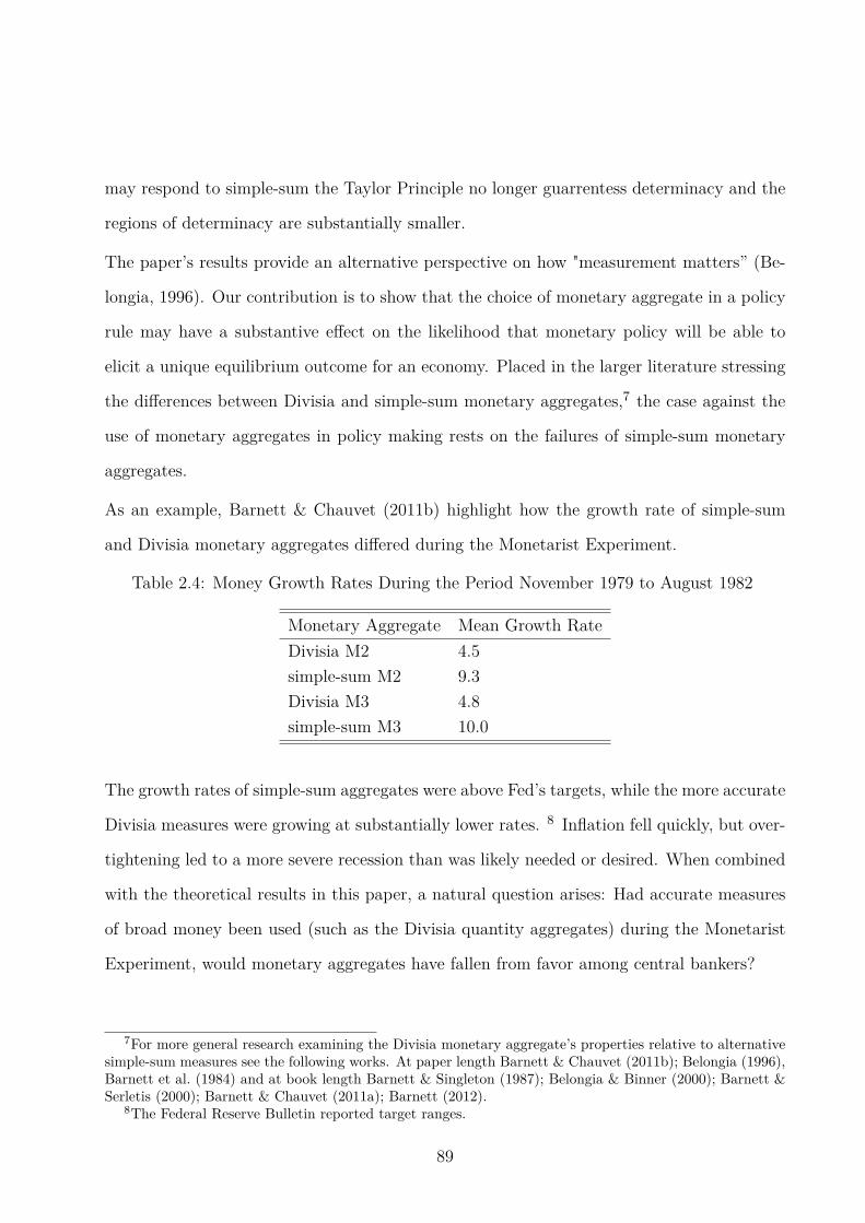
may respond to simple-sum the Taylor Principle no longer guarrentess determinacy and the

regions of determinacy are substantially smaller.

The paper’s results provide an alternative perspective on how "measurement matters” (Be-

longia, 1996). Our contribution is to show that the choice of monetary aggregate in a policy

rule may have a substantive effect on the likelihood that monetary policy will be able to

elicit a unique equilibrium outcome for an economy. Placed in the larger literature stressing

the differences between Divisia and simple-sum monetary aggregates,7 the case against the

use of monetary aggregates in policy making rests on the failures of simple-sum monetary

aggregates.

As an example, Barnett & Chauvet (2011b) highlight how the growth rate of simple-sum

and Divisia monetary aggregates differed during the Monetarist Experiment.

Table 2.4: Money Growth Rates During the Period November 1979 to August 1982

Monetary Aggregate Mean Growth Rate

Divisia M2 4.5

simple-sum M2 9.3

Divisia M3 4.8

simple-sum M3 10.0

The growth rates of simple-sum aggregates were above Fed’s targets, while the more accurate

Divisia measures were growing at substantially lower rates. 8 Inflation fell quickly, but over-

tightening led to a more severe recession than was likely needed or desired. When combined

with the theoretical results in this paper, a natural question arises: Had accurate measures

of broad money been used (such as the Divisia quantity aggregates) during the Monetarist

Experiment, would monetary aggregates have fallen from favor among central bankers?

7For more general research examining the Divisia monetary aggregate’s properties relative to alternativesimple-sum measures see the following works. At paper length Barnett & Chauvet (2011b); Belongia (1996),Barnett et al. (1984) and at book length Barnett & Singleton (1987); Belongia & Binner (2000); Barnett &Serletis (2000); Barnett & Chauvet (2011a); Barnett (2012).

8The Federal Reserve Bulletin reported target ranges.

89

References

Andres, J., Lopez-Salido, J. D., & Nelson, E. (2009). Money and the natural rate of inter-

est: Structural estimates for the united states and the euro area. Journal of Economic

Dynamics and Control, 33(3), 758–776.

Ball, L. (2001). Another look at long-run money demand. Journal of Monetary Economics,

47(1), 31–44.

Barnett, W. A. (1980). Economic monetary aggregates an application of index number and

aggregation theory. Journal of Econometrics, 14(1), 11–48.

Barnett, W. A. (2012). Getting it Wrong: How Faulty Monetary Statistics Undermine the

Fed, the Financial System, and the Economy, volume 1 of MIT Press Books. The MIT

Press.

Barnett, W. A. & Chauvet, M. (2011a). Financial Aggregation And Index Number Theory,

volume 2 of World Scientific Books. World Scientific Publishing Co. Pte. Ltd.

Barnett, W. A. & Chauvet, M. (2011b). How better monetary statistics could have signaled

the financial crisis. Journal of Econometrics, 161(1), 6–23.

Barnett, W. A., Offenbacher, E. K., & Spindt, P. A. (1984). The New Divisia Monetary

Aggregates. Journal of Political Economy, 92(6), 1049–85.

Barnett, W. A. & Serletis, A. (2000). The Theory of Monetary Aggregation. Contributions

to Economic Analysis. Elsevier.

90

Barnett, W. A. & Singleton, K. J. (1987). The microeconomic theory of monetary aggregation.

Cambridge University Press.

Belongia, M. T. (1996). Measurement matters: Recent results from monetary economics

reexamined. Journal of Political Economy, 104(5), 1065–83.

Belongia, M. T. & Binner, J. M. (2000). Divisia Monetary Aggregates: Theory and Practice.

Palgrave.

Belongia, M. T. & Ireland, P. N. (2012). Quantitative Easing: Interest Rates and Money in

the Measurement of Monetary Policy. Boston College Working Papers in Economics 801,

Boston College Department of Economics.

Belongia, M. T. & Ireland, P. N. (2014). The barnett critique after three decades: A new

keynesian analysis. Journal of Econometrics, forthcoming.

Canova, F. & Menz, T. (2011). Does money matter in shaping domestic business cycles? an

international investigation. Journal of Money, Credit and Banking, 43(4), 577–607.

Carlstrom, C. T. & Fuerst, T. S. (1995). Interest rate rules vs. money growth rules a welfare

comparison in a cash-in-advance economy. Journal of Monetary Economics, 36(2), 247–

267.

Carlstrom, C. T. & Fuerst, T. S. (2003). Money Growth Rules and Price Level Determinacy.

Review of Economic Dynamics, 6(2), 263–275.

Diewert, W. E. (1976). Exact and superlative index numbers. Journal of Econometrics,

4(2), 115–145.

Divisia, F. (1926). L’indice monetaire et la theorie de la monnaie. Revue d’econ polit, LX(01),

49–81.

Evans, G. W. & Honkapohja, S. (2003). Friedman’s money supply rule vs. optimal interest

rate policy. Scottish Journal of Political Economy, 50(5), 550–566.

91

Fahr, S., Motto, R., Rostagno, M., Smets, F., & Tristani, O. (2013). A monetary policy

strategy in good and bad times: lessons from the recent past. Economic Policy, 28(74),

243–288.

Friedman, M. (1960). A Program for Monetary Stability. Fordham University Press.

Friedman, M. & Schwartz, A. J. (1971). A Monetary History of the United States, 1867-1960.

Princeton University Press.

Gali, J. (2008). Monetary Policy, Inflation, and the Business Cycle: An Introduction to the

New Keynesian Framework. Princeton University Press.

Ireland, P. N. (1996). The Role of Countercyclical Monetary Policy. Journal of Political

Economy, 104(4), 704–23.

Ireland, P. N. (2009). On the welfare cost of inflation and the recent behavior of money

demand. American Economic Review, 99(3), 1040–52.

Keating, J. & Smith, A. L. (2013). Price Versus Financial Stability: A role for money

in Taylor rules? WORKING PAPERS SERIES IN THEORETICAL AND APPLIED

ECONOMICS 201307, University of Kansas, Department of Economics.

Leeper, E. M. (1991). Equilibria under ’active’ and ’passive’ monetary and fiscal policies.

Journal of Monetary Economics, 27(1), 129–147.

McCallum, B. T. (1998). Solutions to linear rational expectations models: a compact expo-

sition. Economics Letters, 61(2), 143–147.

McCallum, B. T. & Nelson, E. (2011). Money and inflation: Some critical issues. In B. M.

Friedman & M. Woodford (Eds.), Handbook of Monetary Economics, volume 3 of Handbook

of Monetary Economics chapter 3, (pp. 97–153). Elsevier.

Newey, W. K. & West, K. D. (1987). A Simple, Positive Semi-definite, Heteroskedasticity

and Autocorrelation Consistent Covariance Matrix. Econometrica, 55(3), 703–08.

92

Sims, C. A. & Zha, T. (2006). Were there regime switches in u.s. monetary policy? American

Economic Review, 96(1), 54–81.

Woodford, M. (2003). Interest and Prices: Foundations of a Theory of Monetary Policy.

Princeton University Press.

93

2.A Appendix: Proofs

In this section we present the proofs to our results stated in the paper. The equilibrium

model we use in this paper is based on the model described in Belongia & Ireland (2014),

however we assume additively separable preferences between consumption and monetary

services allowing us to obtain analytic results for the determinacy regions. Also, to arrive at

the standard dynamic IS and NKPC, we slightly alter the timing of the transactions for the

representative household.

Proposition 2.1

Consider the dynamic system defined by equations (2.1), (2.2), (2.8) and (2.1),

AEt[wt+1] =Bwt+Cst.

A=

1 1 −1 0

0 −β 0 0

0 0 0 1

0 0 ηr 1

B =

1 0 0 0

κ −1 0 0

0 −1 0 1

1 0 0 0

where wt =

[

yet , πt, rt−1, lt−1

]T

and where lt = mt − pt is real money balances. The

system has two non-predetermined variables and two predetermined variables. Therefore,

the system will have a unique rational expectations equilibrium (REE) if, and only if, two

roots λ which satisfy | B−λA |= 0 lie outside the unit circle and remaining two roots lie

94

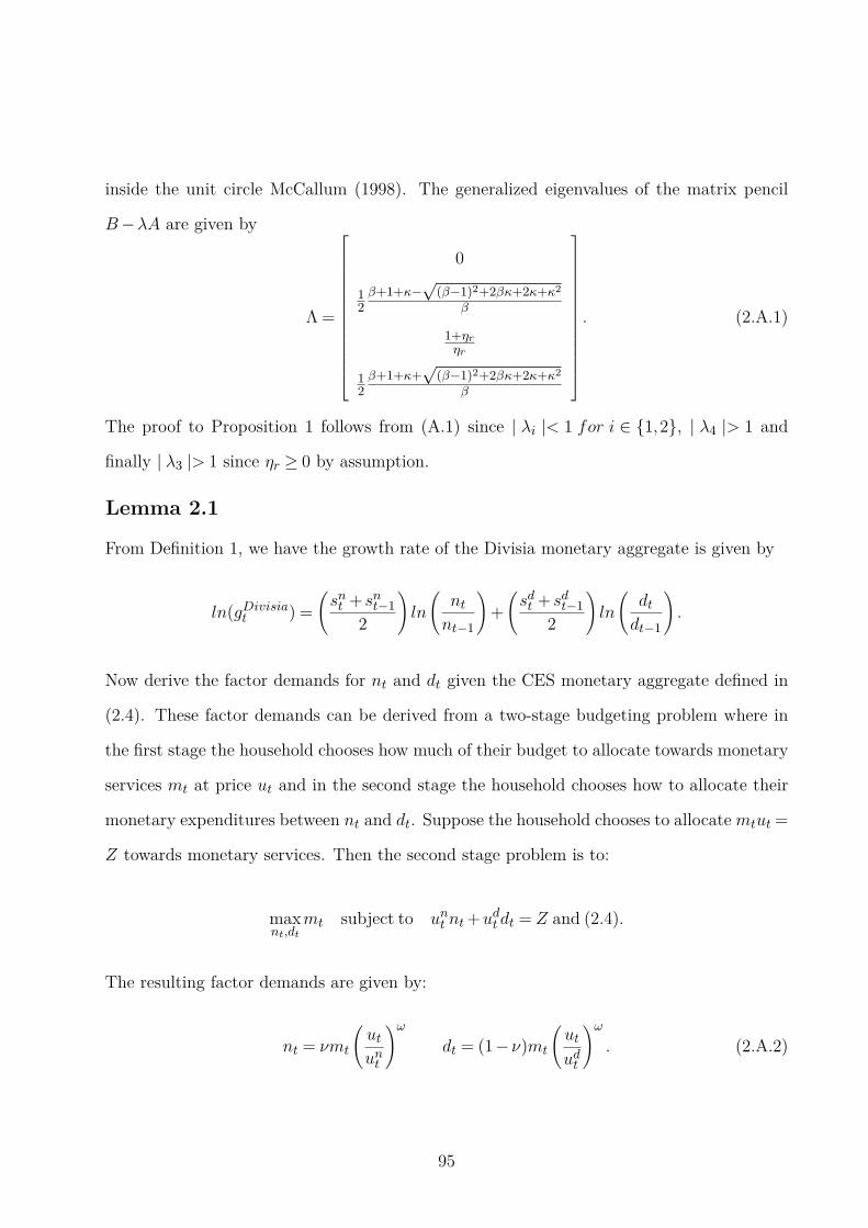
inside the unit circle McCallum (1998). The generalized eigenvalues of the matrix pencil

B−λA are given by

Λ =

0

12β+1+κ−

√(β−1)2+2βκ+2κ+κ2

β

1+ηr

ηr

12β+1+κ+

√(β−1)2+2βκ+2κ+κ2

β

. (2.A.1)

The proof to Proposition 1 follows from (A.1) since | λi |< 1 for i ∈ 1,2, | λ4 |> 1 and

finally | λ3 |> 1 since ηr ≥ 0 by assumption.

Lemma 2.1

From Definition 1, we have the growth rate of the Divisia monetary aggregate is given by

ln(gDivisiat ) =

(

snt + snt−1

2

)

ln

(

ntnt−1

)

+

(

sdt + sdt−1

2

)

ln

(

dtdt−1

)

.

Now derive the factor demands for nt and dt given the CES monetary aggregate defined in

(2.4). These factor demands can be derived from a two-stage budgeting problem where in

the first stage the household chooses how much of their budget to allocate towards monetary

services mt at price ut and in the second stage the household chooses how to allocate their

monetary expenditures between nt and dt. Suppose the household chooses to allocate mtut =

Z towards monetary services. Then the second stage problem is to:

maxnt,dt

mt subject to unt nt+udt dt = Z and (2.4).

The resulting factor demands are given by:

nt = νmt

(

utunt

)ω

dt = (1−ν)mt

(

ut

udt

)ω

. (2.A.2)

95

which satisfy the constraint unt nt+udt dt = utmt for

ut =

ν(rt−1

rt

)1−ω

+(1−ν)

(

rt− rdtrt

)1−ω

11−ω

.

Substituting these factor demands into the definition of the Divisia monetary aggregate,

we obtain the following useful expression for the difference between the growth rates of the

Divisia monetary aggregate and the true monetary aggregate:

ln(gdivisiat )−∆ln(mt)

= ω[

∆ln(

ut(unt ,u

dt ))

− 1

2

(

snt + snt−1

)

∆ln(unt )− 1

2

(

sdt + sdt−1

)

∆ln(

udt)]

≡ EDiv(ln(unt ), ln(udt ), ln(unt−1), ln(udt−1)),

where EDiv is the error-term which quantifies the difference between the Divisia monetary

aggregate and the true monetary aggregate.

To verify the claim, take a first-order Taylor approximation of EDiv around the steady-state,

hence all derivatives below are evaluated at the steady-state.

EDiv =

[

∂EDiv

∂ln(unt )

]

unt +

[

∂EDiv

∂ln(udt )

]

udt +

[

∂EDiv

∂ln(unt−1)

]

unt−1 +

[

∂EDiv

∂ln(udt−1)

]

udt−1 +O(‖ξ‖2)

=

[

∂EDiv

∂ln(unt )

]

unt +

[

∂EDiv

∂ln(udt )

]

udt −[

∂EDiv

∂ln(unt )

]

unt−1 −[

∂EDiv

∂ln(udt )

]

udt−1 +O(‖ξ‖2)

=

[

∂EDiv

∂ln(unt )

]

∆unt +

[

∂EDiv

∂ln(udt )

]

∆udt +O(‖ξ‖2)

Finally, notice that

96

[

∂EDiv

∂ln(unt )

]

=

[

∂ln(ut)

∂ln(unt )− 1

2(snt + snt−1)

]

=ν (un)1−ω

ν (un)1−ω +(1−ν)(

ud)1−ω − ν (un)1−ω

(u)1−ω = 0

and

[

∂EDiv

∂ln(udt )

]

=

[

∂ln(ut)

∂ln(udt )− 1

2(sdt + sdt−1)

]

=(1−ν)

(

ud)1−ω

ν (un)1−ω +(1−ν)(

ud)1−ω −

(1−ν)(

ud)1−ω

(u)1−ω = 0

which verifies our claim since we have ln(gdivisiat )−∆ln(mt) = O(‖ξ‖2).

Lemma 2.2

Much like the proof of Lemma 1, substitute the factor demands for currency and deposits

defined in equation (2.A.2) into the definition of the simple-sum aggregate in definition 2 to

arrive at

ln(gsimple−sumt )−∆ln(mt)

= ω∆ln(ut(unt ,u

dt ))+∆ln(ν(unt )−ω +(1−ν)(udt )

−ω)

≡ ESS(ln(unt ), ln(udt ), ln(unt−1), ln(udt−1)),

where ESS is the error-term which quantifies the difference between the simple-sum monetary

aggregate and the true monetary aggregate.

To verify the claim, take a first-order Taylor approximation of ESS around the steady-state,

97

hence all derivatives below are evaluated at the steady-state.

ESS =

[

∂ESS

∂ln(unt )

]

unt +

[

∂ESS

∂ln(udt )

]

udt +

[

∂ESS

∂ln(unt−1)

]

unt−1 +

[

∂ESS

∂ln(udt−1)

]

udt−1 +O(‖ξ‖2)

=

[

∂ESS

∂ln(unt )

]

unt +

[

∂ESS

∂ln(udt )

]

udt −[

∂ESS

∂ln(unt )

]

unt−1 −[

∂ESS

∂ln(udt )

]

udt−1 +O(‖ξ‖2)

=

[

∂ESS

∂ln(unt )

]

∆unt +

[

∂ESS

∂ln(udt )

]

∆udt +O(‖ξ‖2)

= ω

[

∂ln(ut)

∂ln(unt )− ∂ln(ν(unt )−ω +(1−ν)(udt )

−ω)

∂ln(unt )

]

∆unt

+ω

[

∂ln(ut)

∂ln(udt )− ∂ln(ν(unt )−ω +(1−ν)(udt )

−ω)

∂ln(udt )

]

∆udt +O(‖ξ‖2)

= ω

[

sn− ν(un)−ω

ν(un)−ω +(1−ν)(ud)−ω

]

∆unt

+ω

[

sd− (1−ν)(ud)−ω

ν(un)−ω +(1−ν)(ud)−ω

]

∆udt +O(‖ξ‖2)

= ω

[

ν(un)1−ω

ν(un)1−ω +(1−ν)(ud)1−ω− ν(un)−ω

ν(un)−ω +(1−ν)(ud)−ω

]

∆unt

+ω

[

(1−ν)(ud)1−ω

ν(un)1−ω +(1−ν)(ud)1−ω− (1−ν)(ud)−ω

ν(un)−ω +(1−ν)(ud)−ω

]

∆udt +O(‖ξ‖2)

Let α= ud/un ∈ (0,1), then we have

ESS = ω

[

ν(α)ω−1

ν(α)ω−1 +(1−ν)− ν(α)ω

ν(α)ω +(1−ν)

]

∆unt

+ω

[

(1−ν)

ν(α)ω−1 +(1−ν)− (1−ν)

ν(α)ω +(1−ν)

]

∆udt +O(‖ξ‖2)

= ω

[

ν(α)ω−1(ν(α)ω +(1−ν))−ν(α)ω(ν(α)ω−1 +(1−ν))

(ν(α)ω +(1−ν))(ν(α)ω−1 +(1−ν))

]

∆unt

+ω

[

(1−ν)(ν(α)ω +(1−ν))− (1−ν)(ν(α)ω−1 +(1−ν))

(ν(α)ω +(1−ν))(ν(α)ω−1 +(1−ν))

]

∆udt +O(‖ξ‖2).

98

Further simplifying this expression, we have:

ESS = ω

[

αω[(α)−1ν(1−ν)−ν(1−ν)]

(ν(α)ω +(1−ν))(ν(α)ω−1 +(1−ν))

][

1

r−1−(

τ − x

(r−1)(τ(r−1)+ x)

)]

∆rt

−ω

[

αω[(α)−1ν(1−ν)−ν(1−ν)]

(ν(α)ω +(1−ν))(ν(α)ω−1 +(1−ν))

][(τ

α

)

∆τt+

(

x

(r−1)τ + x

)

∆xt

]

+O(‖ξ‖2)

≡ ψ(ω)

[

rx

(r−1)(τ(r−1)+ x)

]

∆rt−ψ(ω)(τ

α

)

∆τt−ψ(ω)

(

x

(r−1)τ + x

)

∆xt+O(‖ξ‖2)

≡ ψr(ω)∆rt−ψτ (ω)∆τt−ψx(ω)∆xt+O(‖ξ‖2).

To complete the proof, first notice that since (τ , x)> 0 we have that ψr(ω)> 0 and moreover

since ψ(ω) > 0 we have that (ψτ (ω),ψx(ω)) ≫ (0,0). Finally, to obtain the limiting result

apply L’Hospital’s rule to the function

h(ω) = ωeωln(α) =ω

e−ωln(α)

to find that limω→∞

h(ω) = 0 which implies limω→∞

ψ(ω) = 0 verifying the claim.

Corollary 2.2

By Lemma 2, the constant simple-sum growth rule implies a policy rule of the form

0 = ∆gsimple−sumt = ∆mt+ψr(ω)∆rt−ψτ (ω)∆τt−ψx(ω)∆xt.

We can rearrange this expression as an interest rate feedback rule.

rt = rt−1 − 1

ψr(ω)∆mt−

ψτ (ω)

ψr(ω)∆τt−

ψx(ω)

ψr(ω)∆xt (2.A.3)

This rule is part of a more general class of rules studied in section 4. More generally, consider

rules of the form

rt = φrrt−1 +φm∆mt

99

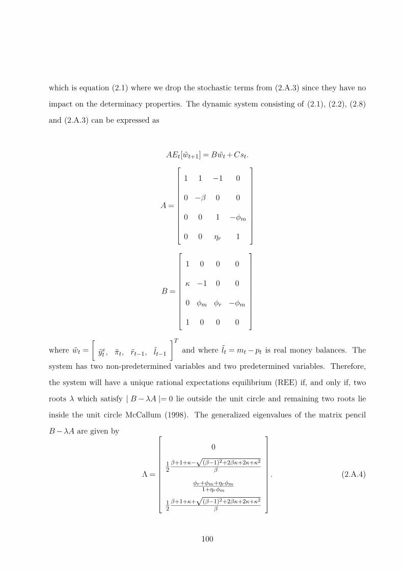
which is equation (2.1) where we drop the stochastic terms from (2.A.3) since they have no

impact on the determinacy properties. The dynamic system consisting of (2.1), (2.2), (2.8)

and (2.A.3) can be expressed as

AEt[wt+1] =Bwt+Cst.

A=

1 1 −1 0

0 −β 0 0

0 0 1 −φm

0 0 ηr 1

B =

1 0 0 0

κ −1 0 0

0 φm φr −φm

1 0 0 0

where wt =

[

yet , πt, rt−1, lt−1

]T

and where lt = mt − pt is real money balances. The

system has two non-predetermined variables and two predetermined variables. Therefore,

the system will have a unique rational expectations equilibrium (REE) if, and only if, two

roots λ which satisfy | B−λA |= 0 lie outside the unit circle and remaining two roots lie

inside the unit circle McCallum (1998). The generalized eigenvalues of the matrix pencil

B−λA are given by

Λ =

0

12β+1+κ−

√(β−1)2+2βκ+2κ+κ2

β

φr+φm+ηrφm

1+ηrφm

12β+1+κ+

√(β−1)2+2βκ+2κ+κ2

β

. (2.A.4)

100

The proof for Corollary 2 follows by letting φr = 1 and φm = − 1ψr(ω) . In which case we have

that | λi |< 1 for i ∈ 1,2, | λ4 |> 1 and finally | λ3 |> 1 if and only if

∣∣∣∣∣

ψr(ω)−ηr −1

ψr(ω)−ηr

∣∣∣∣∣> 1.

This condition will be satisfied if and only if ψr(ω) < ηr + 12 allowing for a possibly infinite

generalized eigenvalue for ψr(ω) = ηr.

Proposition 2.2

This result follows from examining the eigenvalues presented in (3.B.5) above which considers

the dynamic model consisting of (2.1), (2.2), (2.8) and (2.1). We have that | λi |< 1 for i ∈

1,2, | λ4 |> 1 and finally | λ3 |> 1 if and only if

∣∣∣∣∣

φr +φm+ηrφm1+ηrφm

∣∣∣∣∣> 1.

Since we are assuming all terms are non-negative this is equivalent to having that | λ3 |> 1

if and only if φr +φm > 1.

Corollary 2.4

Applying Lemma 2 to the interest rate rule in (2.3) we have the policy rule

rt = φrrt−1 +φss[∆mt+ψr(ω)∆rt−ψτ (ω)∆τt−ψx(ω)∆xt].

Rearranging this expression this expression we have a policy rule of the form

rt =

[

φr −φssψr(ω)

1−φssψr(ω)

]

rt−1 +

[

φss1−φssψr(ω)

]

∆mt (2.A.5)

where we drop the exogenous shock terms since they have no affect on the determinacy

properties of the policy rule. Since the rule in (2.A.5) is of the same general form as (2.1),

we can analyze the eigenvalues in(3.B.5) above. We then have that | λi |< 1 for i ∈ 1,2,

101

| λ4 |> 1 and finally | λ3 |> 1 if and only if

∣∣∣∣∣

φr +φss−φss[ψr(ω)−ηr]

1−φss[ψr(ω)−ηr]

∣∣∣∣∣> 1

or equivalently

|φr +φss−φss[ψr(ω)−ηr]|> |1−φss[ψr(ω)−ηr]|.

102

Chapter 3

A Working Solution to Working

Capital Indeterminacy

3.1 Introduction

The advice to central banks that a well designed interest rate reaction function mechanically

adjusts the policy rate more than one for one to deviations of inflation from target (c.f. Taylor

(1993)) is one of the most robust policy prescriptions in monetary theory. So much so that

leading undergraduate textbooks introduce students to the so called Taylor principle, “The

principle that the monetary authorities should raise nominal interest rates by more than the

increase in the inflation rate has been named the Taylor principle, and it is critical to the

success of monetary policy” (Mishkin, 2013).

However, the Taylor principle as described above is not without its caveats. Importantly,

Christiano et al. (2010) show numerically that an upper bound may need to be placed on the

central bank’s reaction to inflation in order to ensure expectations remain well anchored.1

This upper bound arises when there is a timing mismatch between when the firm produces it

product and when it gets paid for the product. When this occurs, firms will typically have to

1Another apparent failure of the Taylor principle involves the interaction of trend-inflation and determi-nacy. For example, Coibion & Gorodnichenko (2011) show that under the widely used Calvo style pricingassumption and trend inflation, the Taylor principle breaks down.

103

finance inputs with short-term loans called working capital. This environment introduces a

working-capital channel of monetary policy which works counter to the typical transmission

mechanism of monetary policy in New-Keynesian models.2

To illustrate both of these transmission mechanisms, consider for the moment a prototypical

dynamic AS-AD model where expectations are intentionally simplified to allow for graphical

intuition. This model consists of 3 log-linear equations:

yt =− Rt+ εadt

πt =

κyt+βπt−1

κyt+κrRt+βπt−1

Rt =φππt

where the first equation is an IS equation relating cyclical output to the real interest rate

and an exogenous white noise shock, εadt , the second equation is a dynamic Phillip’s curve

relating inflation to cyclical output and possibly the real policy rate if working capital is

required for production and finally the last equation is a simple real interest rate reaction

function which is assumed to describe the behavior of the central bank.

3.1.1 The Taylor Principle: A lower bound on φπ

Assume the typical Phillips curve governs firms’ price setting behavior so that: πt = κyt+

βπt−1. The Taylor principle is represented in the above system as the requirement on the

magnitude of φπ. Since Rt is the real interest rate the, the appropriate condition for a stable

dynamic system φπ > 0. To see why this is so, eliminate Rt from the above system and

plot the resulting aggregate demand and supply curves. Notice that in Figure (3.1a), the

aggregate demand embodies the typical negative relationship between inflation and cyclical

output. This negative relationship emerges from the assumption that φπ > 0 so that when

2Throughout the paper, the terms working-capital channel and cost channel can be used interchangeably.For consistency, I will refer to this mechanism as the working-capital channel.

104

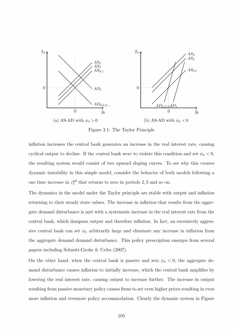
yt

πt

0

AD0,2,3,...

AD1

AS0,1

AS2AS3

0

(a) AS-AD with φπ > 0

yt

πt

0AD0,2,3,...AD1

AS0,1

AS2

AS3

0

(b) AS-AD with φπ < 0

Figure 3.1: The Taylor Principle

inflation increases the central bank generates an increase in the real interest rate, causing

cyclical output to decline. If the central bank were to violate this condition and set φπ < 0,

the resulting system would consist of two upward sloping curves. To see why this creates

dynamic instability in this simple model, consider the behavior of both models following a

one time increase in εad1 that returns to zero in periods 2,3 and so on.

The dynamics in the model under the Taylor principle are stable with output and inflation

returning to their steady state values. The increase in inflation that results from the aggre-

gate demand disturbance is met with a systematic increase in the real interest rate from the

central bank, which dampens output and therefore inflation. In fact, an excessively aggres-

sive central bank can set φπ arbitrarily large and eliminate any increase in inflation from

the aggregate demand demand disturbance. This policy prescription emerges from several

papers including Schmitt-Grohe & Uribe (2007).

On the other hand, when the central bank is passive and sets φπ < 0, the aggregate de-

mand disturbance causes inflation to initially increase, which the central bank amplifies by

lowering the real interest rate, causing output to increase further. The increase in output

resulting from passive monetary policy causes firms to set even higher prices resulting in even

more inflation and evermore policy accommodation. Clearly the dynamic system in Figure

105

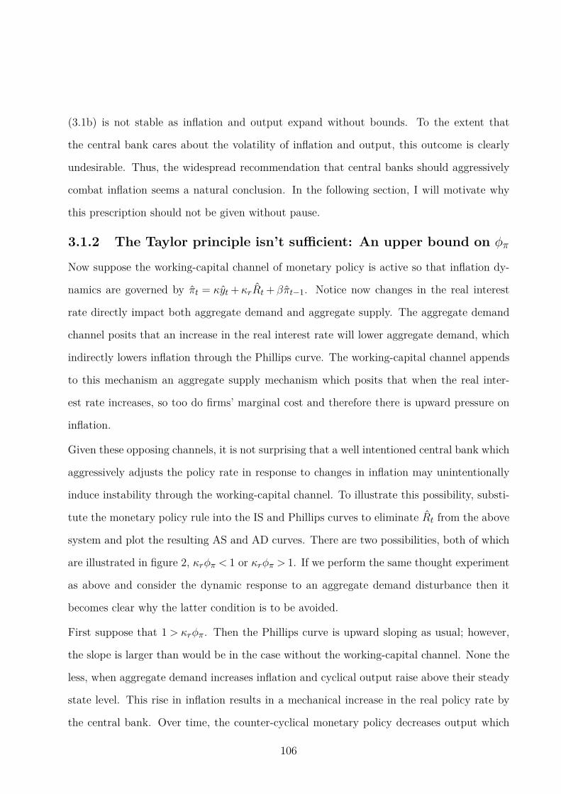
(3.1b) is not stable as inflation and output expand without bounds. To the extent that

the central bank cares about the volatility of inflation and output, this outcome is clearly

undesirable. Thus, the widespread recommendation that central banks should aggressively

combat inflation seems a natural conclusion. In the following section, I will motivate why

this prescription should not be given without pause.

3.1.2 The Taylor principle isn’t sufficient: An upper bound on φπ

Now suppose the working-capital channel of monetary policy is active so that inflation dy-

namics are governed by πt = κyt +κrRt + βπt−1. Notice now changes in the real interest

rate directly impact both aggregate demand and aggregate supply. The aggregate demand

channel posits that an increase in the real interest rate will lower aggregate demand, which

indirectly lowers inflation through the Phillips curve. The working-capital channel appends

to this mechanism an aggregate supply mechanism which posits that when the real inter-

est rate increases, so too do firms’ marginal cost and therefore there is upward pressure on

inflation.

Given these opposing channels, it is not surprising that a well intentioned central bank which

aggressively adjusts the policy rate in response to changes in inflation may unintentionally

induce instability through the working-capital channel. To illustrate this possibility, substi-

tute the monetary policy rule into the IS and Phillips curves to eliminate Rt from the above

system and plot the resulting AS and AD curves. There are two possibilities, both of which

are illustrated in figure 2, κrφπ < 1 or κrφπ > 1. If we perform the same thought experiment

as above and consider the dynamic response to an aggregate demand disturbance then it

becomes clear why the latter condition is to be avoided.

First suppose that 1 > κrφπ. Then the Phillips curve is upward sloping as usual; however,

the slope is larger than would be in the case without the working-capital channel. None the

less, when aggregate demand increases inflation and cyclical output raise above their steady

state level. This rise in inflation results in a mechanical increase in the real policy rate by

the central bank. Over time, the counter-cyclical monetary policy decreases output which

106

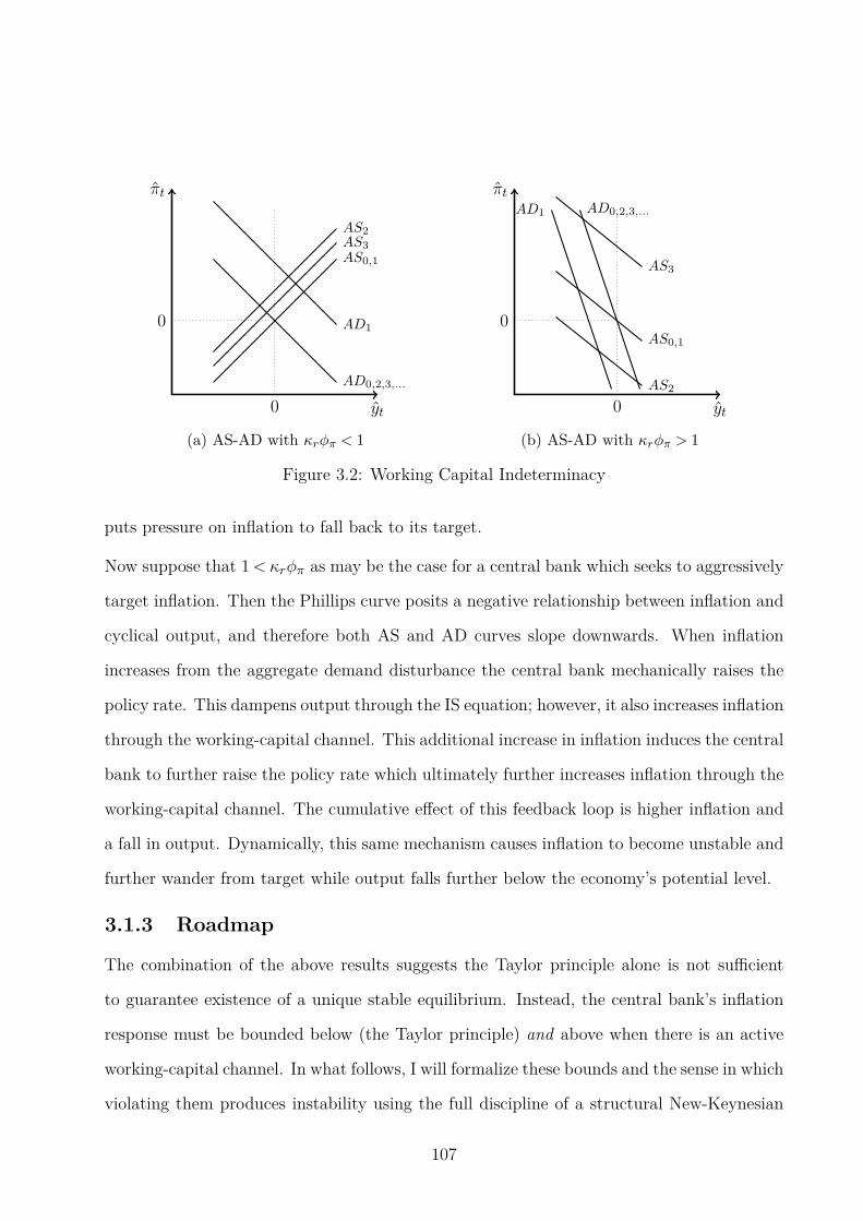
yt

πt

0

AD0,2,3,...

AD1

AS0,1

AS2AS3

0

(a) AS-AD with κrφπ < 1

yt

πt

0

AS0,1

AS2

AS3

AD0,2,3,...AD1

0

(b) AS-AD with κrφπ > 1

Figure 3.2: Working Capital Indeterminacy

puts pressure on inflation to fall back to its target.

Now suppose that 1<κrφπ as may be the case for a central bank which seeks to aggressively

target inflation. Then the Phillips curve posits a negative relationship between inflation and

cyclical output, and therefore both AS and AD curves slope downwards. When inflation

increases from the aggregate demand disturbance the central bank mechanically raises the

policy rate. This dampens output through the IS equation; however, it also increases inflation

through the working-capital channel. This additional increase in inflation induces the central

bank to further raise the policy rate which ultimately further increases inflation through the

working-capital channel. The cumulative effect of this feedback loop is higher inflation and

a fall in output. Dynamically, this same mechanism causes inflation to become unstable and

further wander from target while output falls further below the economy’s potential level.

3.1.3 Roadmap

The combination of the above results suggests the Taylor principle alone is not sufficient

to guarantee existence of a unique stable equilibrium. Instead, the central bank’s inflation

response must be bounded below (the Taylor principle) and above when there is an active

working-capital channel. In what follows, I will formalize these bounds and the sense in which

violating them produces instability using the full discipline of a structural New-Keynesian

107

model and rational expectations. I also show that Friedman’s k-percent money growth rule

and an interest rate rule reacting to money growth with a coefficient satisfying the lower

bound condition φm > 1 are sufficient for determinacy. In other words, the working capital

induced indeterminacy is a potential pitfall exclusive to inflation targeting regimes. I also

show the above determinacy results are robust to weakening the assumption that firms

borrow at the policy rate. Finally, I augment the standard model with real wage rigidities.

This additional friction further restricts the central bank’s reaction to inflation but has no

impact on the determinacy regions of money growth targeting rules.

3.2 DSGE Model

This section describes the DSGE model used in the paper in detail. The model motivates

the working capital channel through a timing mismatch between when firms pay their wage

bill and receive payment for their output. To align the model as much as possible with the

textbook New-Keynesian model, I assume that all financial transactions are intratemporal

and therefore all interest rates are known at the beginning of the period. This allows firms

to adjust their prices before actually paying back their working capital loans at the end of

the period.3

3.2.1 The Household

The representative household enters any period t= 0,1,2, ... with a portfolio consisting of 3

assets. The household holds maturing bonds bt−1 , shares of monopolistically competitive

firm i ∈ [0,1] st−1(i), and base money totaling mbt−1. The household faces a sequence of

budget constraints in any given period. This budgeting can be described by dividing period

t into 2 separate periods: first a securities trading session and then bank settlement period.

In the securities trading session the household can buy and sell stocks, bonds, receives wages

wt for hours worked ht during the period, purchases consumption goods ct and obtains any

loans lhht needed to facilitate these transactions. Any government transfers are also made

3Christiano et al. (2005) provide an alternative timing assumption in which the policy rate (which equalsthe loan rate in their model) is not known when period t prices are set.

108

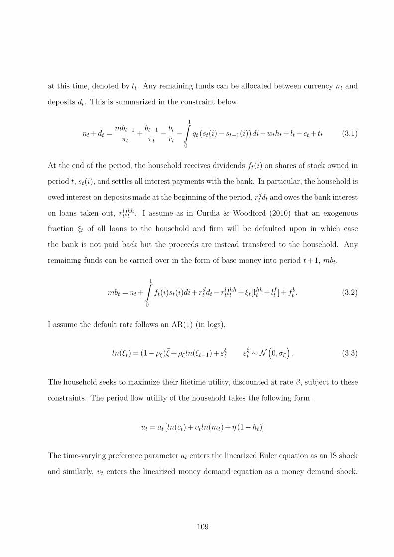
at this time, denoted by tt. Any remaining funds can be allocated between currency nt and

deposits dt. This is summarized in the constraint below.

nt+dt =mbt−1

πt+bt−1

πt− btrt

−1ˆ

0

qt (st(i)− st−1(i))di+wtht+ lt− ct+ tt (3.1)

At the end of the period, the household receives dividends ft(i) on shares of stock owned in

period t, st(i), and settles all interest payments with the bank. In particular, the household is

owed interest on deposits made at the beginning of the period, rdt dt and owes the bank interest

on loans taken out, rltlhht . I assume as in Curdia & Woodford (2010) that an exogenous

fraction ξt of all loans to the household and firm will be defaulted upon in which case

the bank is not paid back but the proceeds are instead transfered to the household. Any

remaining funds can be carried over in the form of base money into period t+1, mbt.

mbt = nt+

1ˆ

0

ft(i)st(i)di+ rdt dt− rltlhht + ξt[ł

hht + lft ]+f bt . (3.2)

I assume the default rate follows an AR(1) (in logs),

ln(ξt) = (1−ρξ)ξ+ρξln(ξt−1)+ εξt εξt ∼ N(

0,σξ)

. (3.3)

The household seeks to maximize their lifetime utility, discounted at rate β, subject to these

constraints. The period flow utility of the household takes the following form.

ut = at [ln(ct)+υtln(mt)+η (1−ht)]

The time-varying preference parameter at enters the linearized Euler equation as an IS shock

and similarly, υt enters the linearized money demand equation as a money demand shock.

109

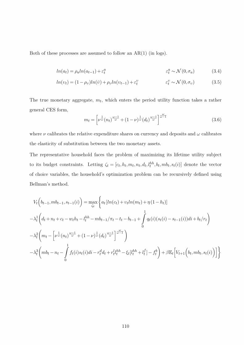
Both of these processes are assumed to follow an AR(1) (in logs).

ln(at) = ρaln(at−1)+ εat εat ∼ N (0,σa) (3.4)

ln(υt) = (1−ρυ)ln(υ)+ρυln(υt−1)+ ευt ευt ∼ N (0,συ) (3.5)

The true monetary aggregate, mt, which enters the period utility function takes a rather

general CES form,

mt =[

ν1ω (nt)

ω−1ω +(1−ν)

1ω (dt)

ω−1ω

] ωω−1

(3.6)

where ν calibrates the relative expenditure shares on currency and deposits and ω calibrates

the elasticity of substitution between the two monetary assets.

The representative household faces the problem of maximizing its lifetime utility subject

to its budget constraints. Letting ζt = [ct,ht,mt,nt,dt, lhht , bt,mbt, st(i)] denote the vector

of choice variables, the household’s optimization problem can be recursively defined using

Bellman’s method.

Vt

(

bt−1,mbt−1, st−1(i))

= maxζt

at [ln(ct)+υtln(mt)+η (1−ht)]

−λ1t

(

dt+nt+ ct−wtht− lhht −mbt−1/πt− tt− bt−1 +

1ˆ

0

qt(i)(st(i)− st−1(i))di+ bt/rt

)

−λ2t

(

mt−[

ν1ω (nt)

ω−1ω +(1−ν)

1ω (dt)

ω−1ω

] ωω−1

)

−λ3t

(

mbt−nt−1ˆ

0

ft(i)st(i)di− rdt dt+ rltlhht − ξt[l

hht + lft ]−f bt

)

+βEt

[

Vt+1

(

bt,mbt, st(i))]

110

The first order necessary conditions are given by the following equations:

atct

= βEt

[

at+1

ct+1

rtπt+1

]

(3.7)

mrst = ηct (3.8)

wt = wρw

t−1mrs(1−ρw)t (3.9)

mt = ct

(

λ2t

λ1t

)−1

υt (3.10)

nt = νmt

[

λ2t /λ

1t

(rt−1)/rt

]ω

(3.11)

dt = (1−ν)mt

[

λ2t /λ

1t

(rt− rdt )/rt

]ω

(3.12)

rlt = rt+ ξt (3.13)

λ1t qt(i) = λ3

t ft(i)+βEt[λ1t+1qt+1(i)]. (3.14)

The above equations are quite standard with a few exceptions. Notice that equations (5.7)

and (5.8) can be combines to yield the typical condition that the real wage equals the

marginal rate of substitution when ρw = 0. However, when 1 > ρw > 0 this condition only

holds in steady state and there may be short-run deviations from this optimality condition

due to real wage rigidity as in Blanchard & Gali (2007).

Additionally, the demand for the monetary aggregate and the various component quantities

shows that when money is modeled as an aggregate of imperfectly substitutable assets, the

demand for the aggregate and each component asset doesn’t depend exclusively on the short

term policy rate as is typically the case in the standard New-Keynesian economies (see

for e.g. Woodford (1999) and Gali (2008)). Instead, these demand functions depend on

the relative user costs of currency, deposits and the monetary aggregate: unt = (rt − 1)/rt,

udt = (rt − rdt )/rt and ut = λ2t /λ

1t . Finally, notice the loan rate deviates from the rate on

1-period bonds by the default rate, giving rise to a time varying finance premium driven

default rates.

111

3.2.2 The Goods Producing Sector

The goods producing sector features a final goods firm and an intermediate goods firm.

There are a unit measure of intermediate goods producing firms indexed by i ∈ [0,1] who

produce a differentiated product. The final goods firm produces yt combining inputs yt(i)

using the constant returns to scale technology,

yt =

1ˆ

0

yt(i)θt−1

θt di

θtθt−1

in which θt > 1 governs the elasticity of substitution between inputs, yt(i). As in Smets &

Wouters (2007), I assume this elasticity is time varying:

ln(θt) = (1−ρθ)θ+ρθln(θt−1)+ εθt εθt ∼ N (0,σθ) , (3.15)

which results in pure cost-push shocks in the New-Keynesian Phillips curve. The final goods

producing firm sells its product in a perfectly competitive market, hence solving the profit

maximization problem,

maxyt(i)i∈[0,1]

pt

1ˆ

0

yt(i)θt−1

θt di

θtθt−1

−1ˆ

0

pt(i)yt(i)di.

The resulting first order condition defines the demand curve for each intermediate goods

producing firm’s product.

yt(i) =

(

pt(i)

pt

)−θt

yt (3.16)

Intermediate Goods Producing Firm

Given the downward sloping demand for its product in (3.16), the intermediate goods pro-

ducing firm has the ability to set the price of its product above marginal cost. Unlike the

112

final goods market, the intermediate goods market is not purely competitive as evident by

the downward sloping demand for its product in equation (3.16). To permit aggregation and

allow for the consideration of a representative intermediate goods producing firm i, I assume

all such firms have the same constant returns to scale technology which implies linearity in

the single input labor ht(i),

yt(i) = ztht(i). (3.17)

The zt term in (3.17) is an aggregate technology shock that follows an AR(1) in log differ-

ences,

ln(zt/zt−1) = (1−ρz)z+ρzln(zt−1/zt−2)+ εzt εzt ∼ N (0,σz) . (3.18)

The price setting ability of each firm is constrained in two ways. First, each intermediate

goods producing firm faces a demand for its product from the representative final goods

producing firm defined in (3.16). Second, each intermediate goods producing firm faces a

convex cost of price adjustment proportional one unit of the final good defined by Rotemberg

(1982) to take the form,

Φ(pt(i),pt−1(i),pt,yt) =φ

2

[

pt(i)

πpt−1(i)−1

]2

yt.

The intermediate goods producing firm maximizes its period t real stock price, qt(i). Using

the representative household’s demand for firm i′s stock (3.14) and iterating forward defines

the real (no-bubbles) share price as the discounted sum of future dividend payments,

qt(i) = Et

∞∑

j=0

βjλ3t+j

λ1tft+j(i)

.

Though the firm maximizes period t share price, the costly price adjustment constraint makes

the intermediate goods producing firm’s problem dynamic. Mathematically summarizing,

113

each intermediate goods producing firm solves to following dynamic problem.

maxyt(i),ht(i),pt(i)∞

t=0

Et

∞∑

j=0

βjλ3t+j

λ1t

pt(i)

ptyt(i)− rltwtht(i)− φ

2

[

pt(i)

πpt−1(i)−1

]2

yt

subject to

yt(i) =

[

pt(i)

pt

]−θt

yt

yt(i) = ztht(i)

The presence of the gross nominal loan rate in the firm’s profit function is the result of

the timing assumption which stipulates that firms must finance inputs with working capital

loans before being paid for their output. In this case, the firm borrows their entire wage bill

each period:

lft (i) = wtht(i). (3.19)

After paying the loan back with interest the firms total cost of obtaining inputs is given by

rltlft (i)− lft (i)+wtht(i) = rltwtht(i) where the equality follows from (3.19).

The problem can be simplified by substituting the inverse of the technology constraint for

ht(i) and then substituting the factor demand into the resulting expression for yt(i) so

that now the representative intermediate goods producing firm solves the following recursive

problem defined by Bellman’s equation.

Vt(pt−1(i)) = maxpt(i)

λ3t ytλ1t

[

pt(i)

pt

]1−θt

− rltwtzt

[

pt(i)

pt

]−θt

− φ

2

[

pt(i)

πpt−1(i)−1

]2

+βEt

[

Vt+1(pt(i))]

114

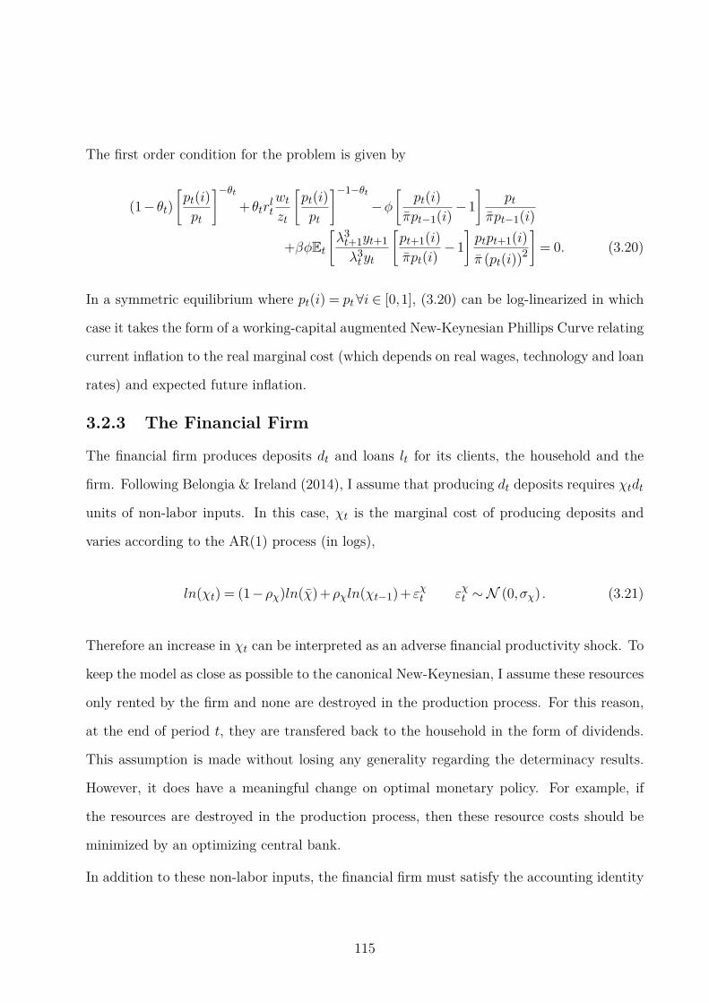
The first order condition for the problem is given by

(1− θt)

[

pt(i)

pt

]−θt

+ θtrltwtzt

[

pt(i)

pt

]−1−θt

−φ

[

pt(i)

πpt−1(i)−1

]

ptπpt−1(i)

+βφEt

[

λ3t+1yt+1

λ3t yt

[

pt+1(i)

πpt(i)−1

]

ptpt+1(i)

π (pt(i))2

]

= 0. (3.20)

In a symmetric equilibrium where pt(i) = pt∀i ∈ [0,1], (3.20) can be log-linearized in which

case it takes the form of a working-capital augmented New-Keynesian Phillips Curve relating

current inflation to the real marginal cost (which depends on real wages, technology and loan

rates) and expected future inflation.

3.2.3 The Financial Firm

The financial firm produces deposits dt and loans lt for its clients, the household and the

firm. Following Belongia & Ireland (2014), I assume that producing dt deposits requires χtdt

units of non-labor inputs. In this case, χt is the marginal cost of producing deposits and

varies according to the AR(1) process (in logs),

ln(χt) = (1−ρχ)ln(χ)+ρχln(χt−1)+ εχt εχt ∼ N (0,σχ) . (3.21)

Therefore an increase in χt can be interpreted as an adverse financial productivity shock. To

keep the model as close as possible to the canonical New-Keynesian, I assume these resources

only rented by the firm and none are destroyed in the production process. For this reason,

at the end of period t, they are transfered back to the household in the form of dividends.

This assumption is made without losing any generality regarding the determinacy results.

However, it does have a meaningful change on optimal monetary policy. For example, if

the resources are destroyed in the production process, then these resource costs should be

minimized by an optimizing central bank.

In addition to these non-labor inputs, the financial firm must satisfy the accounting identity

115

which specifies assets (loans to households and firms plus reserves) equal liabilities (deposits),

lt+ τtdt = dt. (3.22)

Although changes in banking regulation have effectively eliminated reserve requirements,

banks may often choose to hold reserves in lieu of making loans - a flight to quality of sorts.

Therefore, instead of assuming the central bank controls the reserve ratio τt, assume it varies

exogenously according to the AR(1) process (in logs),

ln(τt) = (1−ρτ )ln(τ)+ρτ ln(τt−1)+ ετt ετt ∼ N (0,στ ) . (3.23)

An increase in τt can therefore be interpreted as a reserves demand shock, as opposed to a

change in policy.

The financial firm chooses lt and dt in order to maximize period profits

maxlt,dt

(1− ξt)rltlt− rdt dt− lt+dt−χtdt

subject to the balance sheet constraint (3.22). Since the loan and deposits markets are

perfectly competitive, substiuting the balance-sheet constraint into the profit function and

imposing zero profits due to the perfect competition in the banking sector results in the

loan-deposit spread,

rlt− rdt = rltξt+[rlt(1− ξt)−1]τt+χt. (3.24)

To understand this expression, notice the first term captures the revenues lost to non-

performing loans while the second term captures the foregone revenue of making loans (net

of defaults) when deposits are held as reserves instead of being loaned out. The last term is

the cost of renting χtdt units of the final good to produce dt deposits.

116

3.2.4 Central Bank Policy

As is standard in New-Keynesian economies, the system of equations is under determined

without a specification of monetary policy. The goal is this paper is to understand how the

working-capital channel impacts the determinacy regions of various policy rules. One of the

most widely prescribed policy rules (see for e.g. Schmitt-Grohe & Uribe (2007)) is given by

the simple feedback rule:(rtr

)

=(πtπ

)φπ

eεrt .

For values of φπ sufficiently large, this rule can deliver welfare performance arbitrarily close

to optimal Ramsey policies in New-Keynesian models (see for e.g. Faia & Monacelli (2007)).

After showing rules these inflation targeting interest rate rules are subject to both lower and

upper bounds on φπ, I provide analogous results which show that rules reacting the growth

rate of money can achieve determinacy under less stringent conditions. In particular, the

money growth targeting rule is defined by:

(rtr

)

=(rtr

)φr(

mt

mt−1

πtπ

)φm

eεrt .

This rule is only subject to a lower bound condition φr +φm > 1 regardless of the strength

of the working-capital channel.

Given that Friedman (1960) to alluded a similar rule to implement his famous k-percent

rule:

mt

mt−1

πtπ

= (1+k)eεrt (3.25)

it is perhaps not surprising that Friedman’s k-percent rule is also always determinate, re-

gardless of the strength of the working-capital channel.

Although these rules are of interest for understanding the design of policy rules, it is more

widely believed actual Federal reserve policy is best described by a Taylor (1993) rule since

117

the late 1980’s (Thornton (2012) provides narrative evidence to this point):

(rtr

)

=(πtπ

)φπ(xtx

)φx

eεrt ,

where xt is the output gap, the difference between output and the potential level of output.

In this economy, this level of output can be characterized by the efficient level output. In

other words, the level of output arising from the frictionless problem:

maxct,ht(i)

at[ln(ct)+η(1−1ˆ

0

ht(i)di)] subject to ct = zt

(

ht(i)θt−1

θt

) θtθt−1

.

The resulting first order condition yields the efficient level of output: y∗t = c∗t = zt/η, which

yields the follow expression for the efficient output gap, deonted by xt:

xt =yty∗t

= ηytzt. (3.26)

These various interest rate rules can be concisely embedded in the generalized interest rate

rule:(rtr

)

=(rtr

)ρr(

mt

mt−1

πtπ

)φm (πtπ

)φπ(xtx

)φx

eεrt . (3.27)

3.2.5 Market Clearing

It is now possible to define the equilibrium conditions which close the model. Equilibrium

in the final goods market requires that the accounting identity

yt = ct+φ

2

[πtπ

−1]2

yt (3.28)

118

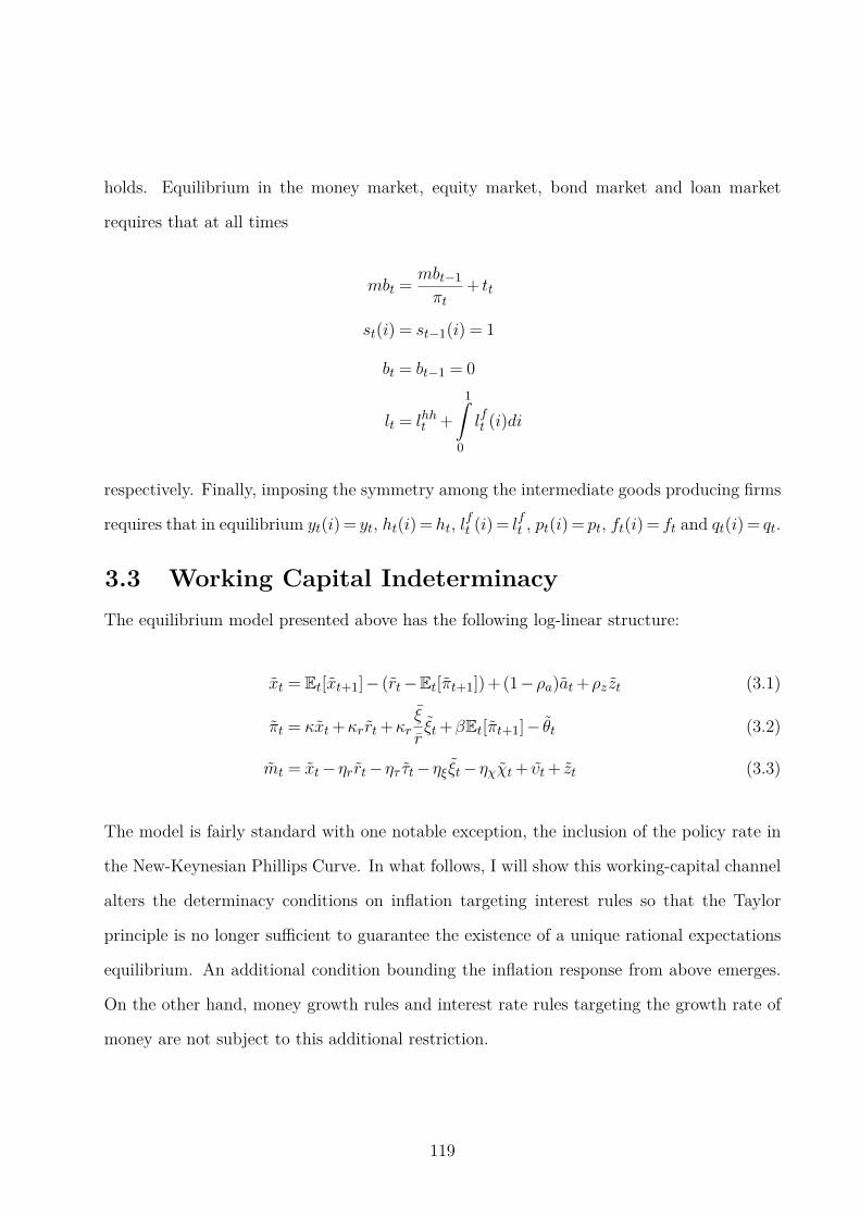
holds. Equilibrium in the money market, equity market, bond market and loan market

requires that at all times

mbt =mbt−1

πt+ tt

st(i) = st−1(i) = 1

bt = bt−1 = 0

lt = lhht +

1ˆ

0

lft (i)di

respectively. Finally, imposing the symmetry among the intermediate goods producing firms

requires that in equilibrium yt(i) = yt, ht(i) = ht, lft (i) = lft , pt(i) = pt, ft(i) = ft and qt(i) = qt.

3.3 Working Capital Indeterminacy

The equilibrium model presented above has the following log-linear structure:

xt = Et[xt+1]− (rt−Et[πt+1])+ (1−ρa)at+ρz zt (3.1)

πt = κxt+κrrt+κrξ

rξt+βEt[πt+1]− θt (3.2)

mt = xt−ηrrt−ητ τt−ηξ ξt−ηχχt+ υt+ zt (3.3)

The model is fairly standard with one notable exception, the inclusion of the policy rate in

the New-Keynesian Phillips Curve. In what follows, I will show this working-capital channel

alters the determinacy conditions on inflation targeting interest rules so that the Taylor

principle is no longer sufficient to guarantee the existence of a unique rational expectations

equilibrium. An additional condition bounding the inflation response from above emerges.

On the other hand, money growth rules and interest rate rules targeting the growth rate of

money are not subject to this additional restriction.

119

3.3.1 Inflation targeting when wages are flexible

In this section, I analyze the conditions for equilibrium existence and uniqueness when the

central bank targets inflation. Inflation targeting is a particularly interesting policy regime

to analyze since it has been implemented to some degree by numerous central banks.4 Strict

Inflation Targeting of the sorts advocated by Svensson (1999) can be defined by the targeting

rule:

πt = 0 (3.4)

The practice of this sort of policy is well supported by the findings in many New-Keynesian

models. For example, Woodford (1999) (pg. 290) shows that such a criterion replicates many

desirable aspects of optimal monetary policy, including determinacy. However, the following

proposition shows this result is not robust to the inclusion of a working-capital channel.

Proposition 3.1. For ρw = 0, for any 0 < β < 1, for any κ > 0 and for any κ ≥ κr ≥ 0 if

the central bank follows the policy rule πt = 0 then there exists a unique REE if and only if

κr <12κ.

Unless noted otherwise, all proofs are in the appendix. Proposition (3.1) shows that if a

central bank is committed in the most extreme sense to achieving their inflation target then

equilibrium determinacy is unlikely, unless the working-capital channel is sufficiently weak.

One interesting case, which has received the bulk of attention in the cost-channel literature

is κr = κ. This emerges as a special case in this model when ξt = 0 which then implies rt = rlt.

The interpretation of this assumption is that firms borrow at the central bank’s policy rate.

In this restricted case, strict inflation targeting leads to indeterminacy. However, Proposition

(3.1) shows that in a more general case where the loan rate differs from the policy rate, the

condition for equilibrium determinacy depends on the degree to which the loan rate varies

with the policy rate. In Section (3.4), I will show that assuming κr = κ is not far from

4The clearest example is New Zealand which officially adopted inflation targeting in 1990. See Roger(2010) for a full list of known inflation targeting central banks.

120

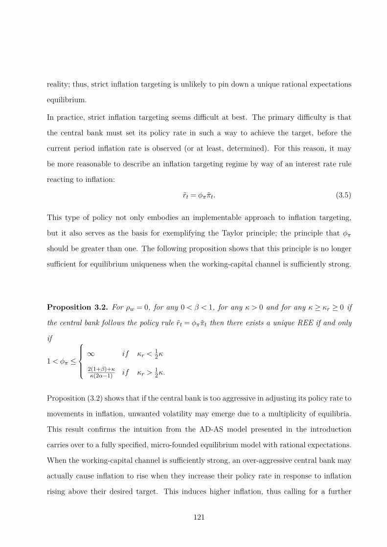
reality; thus, strict inflation targeting is unlikely to pin down a unique rational expectations

equilibrium.

In practice, strict inflation targeting seems difficult at best. The primary difficulty is that

the central bank must set its policy rate in such a way to achieve the target, before the

current period inflation rate is observed (or at least, determined). For this reason, it may

be more reasonable to describe an inflation targeting regime by way of an interest rate rule

reacting to inflation:

rt = φππt. (3.5)

This type of policy not only embodies an implementable approach to inflation targeting,

but it also serves as the basis for exemplifying the Taylor principle; the principle that φπ

should be greater than one. The following proposition shows that this principle is no longer

sufficient for equilibrium uniqueness when the working-capital channel is sufficiently strong.

Proposition 3.2. For ρw = 0, for any 0 < β < 1, for any κ > 0 and for any κ ≥ κr ≥ 0 if

the central bank follows the policy rule rt = φππt then there exists a unique REE if and only

if

1< φπ ≤

∞ if κr <12κ

2(1+β)+κκ(2α−1) if κr >

12κ.

Proposition (3.2) shows that if the central bank is too aggressive in adjusting its policy rate to

movements in inflation, unwanted volatility may emerge due to a multiplicity of equilibria.

This result confirms the intuition from the AD-AS model presented in the introduction

carries over to a fully specified, micro-founded equilibrium model with rational expectations.

When the working-capital channel is sufficiently strong, an over-aggressive central bank may

actually cause inflation to rise when they increase their policy rate in response to inflation

rising above their desired target. This induces higher inflation, thus calling for a further

121

mechanical increase in the policy rate leading to ultimately higher inflation and higher policy

rates. Once again, the additional constraint on the policy marker’s reaction to inflation only

emerges when κr >12κ. As I show later, this is the empirically relevant case.

3.3.2 Money growth targeting when wages are flexible

This section shows inflation targeting rules are particularly susceptible to this working-

capital feedback loop. I reach this conclusion by showing that rules which target the growth

rate of the monetary aggregate have stable determinacy regions independent of the strength

of the working-capital channel. Although money growth oriented rules have fallen from

favor amongst central bankers, they have a rich history in monetary theory. Arguably, all

policy rules trace their roots to Friedman’s k-percent money growth rule which called for

the central bank to fix the growth rate of a broad monetary aggregate (such as M2) at k-

percent. Friedman argued that doing so shielded the economy from potential mistakes by

central bankers, such as passively allowing the money supply to collapse, a chief explanation

for the severity of the Great Depression according to Milton Friedman and Anna Schwartz

(1971).

Instead of preventing a central bank from becoming too passive, in what follows I show that

money growth rules shield the economy from an overly active central banker. In particular,

if inflation rises above target, a central bank which attempts to stabilize the growth rate of

nominal money will react by increasing interest rates (since nominal money growth implicitly

includes inflation). However, the increase in nominal rates decreases the demand for money.

This opposing effect tempers the central bank’s contraction, preventing the possibility of

sunspot equilibria emerging regardless of the strength of the working-capital channel.

Proceeding in a similar fashion as above, first consider a strict money growth target as

proposed by Friedman (1960) whereby each period the central bank sets the growth rate of

money to the desired rate of k-percent:

∆mt+ πt = 0, (3.6)

122

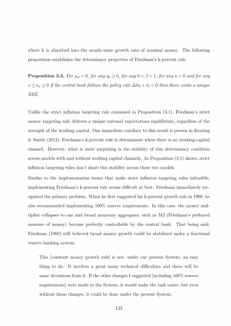
where k is absorbed into the steady-state growth rate of nominal money. The following

proposition establishes the determinacy properties of Friedman’s k-percent rule.

Proposition 3.3. For ρw = 0, for any ηr ≥ 0, for any 0< β < 1, for any κ > 0 and for any

κ≥ κr ≥ 0 if the central bank follows the policy rule ∆mt+ πt = 0 then there exists a unique

REE.

Unlike the strict inflation targeting rule examined in Proposition (3.1), Friedman’s strict

money targeting rule delivers a unique rational expectations equilibrium, regardless of the

strength of the working capital. One immediate corollary to this result is proven in Keating

& Smith (2013), Friedman’s k-percent rule is determinate when there is no working-capital

channel. However, what is more surprising is the stability of this determinacy condition

across models with and without working capital channels. As Proposition (3.1) shows, strict

inflation targeting rules don’t share this stability across these two models.

Similar to the implementation issues that make strict inflation targeting rules infeasible,

implementing Friedman’s k-percent rule seems difficult at best. Friedman immediately rec-

ognized the primary problem. When he first suggested his k-percent growth rule in 1960, he

also recommended implementing 100% reserve requirements. In this case, the money mul-

tiplier collapses to one and broad monetary aggregates, such as M2 (Friedman’s preferred

measure of money) become perfectly controllable by the central bank. That being said,

Friedman (1960) still believed broad money growth could be stabilized under a fractional

reserve banking system:

This [constant money growth rule] is not, under our present System, an easy

thing to do. It involves a great many technical difficulties and there will be

some deviations from it. If the other changes I suggested [including 100% reserve

requirements] were made in the System, it would make the task easier; but even

without those changes, it could be done under the present System.

123

In fact, Friedman believed the stability in the U.S. economy that preceded the financial crisis

was due in large part to the Federal Reserve’s ability to stabilize the growth rate of money

by using the short-term interest rate. This is evident from the following exchange between

Milton Friedman and Russ Roberts in an EconTalk interview in September, 2006.5

Russ Roberts: [Shortly after A Monetary History of the United States, 1867-

1960 was published the central bank’s role was focused on the money supply.]

Something changed in the last 25 or 30 years. That’s not what Alan Greenspan

or Ben Bernanke talk about. They talk about other things and they play with

that short-term interest rate, not the so-called stock of money that you focused

on so intensely in the book.

Friedman: That’s what they talk about but that’s not what they do.

Russ Roberts: What do they do?

Friedman: They use the short-term interest rate as a way of controlling the

quantity of money.

Clearly this interpretation of monetary policy over the great moderation is not consistent

with FOMC transcripts or most of the monetary policy research.6 None the less, it provides

an interesting point to consider the monetary policy rule:

rt = ρrrt−1 +φm(∆mt+ πt) (3.7)

as it should be feasible for the central bank to adjust the short term policy rate to achieve its

desired nominal money growth rate. Although money growth targeting rules are typically

considered inferior to inflation targeting rules from a normative perspective, the following

proposition shows this conclusion may be premature.

5Friedman passed away just two months later, on November 16th.6See for example Kahn & Benolkin (2007) and the quote within from Lawrence Meyer, former Federal

Reserve Governor, “money plays no role in today’s consensus macro model ... and virtually no role in theconduct of monetary policy, at least in the United States." Moreover, Woodford’s (1999) “cashless” economymodels of monetary policy are pervasively used by academic and central bank researchers.

124

Proposition 3.4. For ρw = 0, for any ηr ≥ 0, for any 0< β < 1, for any κ > 0 and for any

κ ≥ κr ≥ 0 if the central bank follows the policy rule rt = ρrrt−1 +φm(∆mt+ πt) then there

exists a unique REE if and only if ρr +φm > 1.

Proposition (3.4) shows that money growth targeting rules satisfy a Taylor principle of their

own sorts. In particular, adjusting the policy rate more than one percentage point for each

one percentage point deviation of nominal money growth from the desired target. This sim-

ple sufficient condition is robust to models with and without the working-capital channel.

Furthermore, in the numerical analysis that follows, I show this condition is sufficient to

anchor expectations on a unique rational expectations equilibrium even when a strong re-

sponse to inflation is added. Hence, aggressive inflation targeting can be implemented once

the central bank is sufficiently committed to stabilizing money growth.

Implementing money growth targeting does face a potential shortcoming relative to inflation

targeting. In particular, the policy rules in Propositions (3.3) and (3.4) require the central

bank to control a monetary aggregate which contains unknown structural parameters such

as ν and ω. A similar issue emerges in small open New-Keynesian models where the CPI

price index is typically modeled as a CES aggregate or domestic and foreign goods. Just as

chain weighted index numbers are used in practice to calculate CPI figures, index number

theory can be combined with monetary aggregation theory to construct a monetary index.

Barnett (1978, 1980) made this possible by deriving the expression for the user-costs of

monetary assets which can then be combined with data on the quantity of each assets to

create a chain-weighted index number. The result is the Divisia monetary aggregate (index)

which is defined as follow in this model economy.

Definition 3.1. The growth rate of the nominal Divisia monetary aggregate is defined by

ln(µt) =

(

snt + snt−1

2

)

ln

(

ntnt−1

)

+

(

sdt + sdt−1

2

)

ln

(

dtdt−1

)

+ ln(πt), (3.8)

125

where snt and sdt are the expenditure shares of currency and interest bearing deposits respec-

tively defined by:

snt =unt nt

unt nt+udt dt=

[(rt−1)/rt]nt

[(rt−1)/rt]nt+[(rt− rdt )/rt]dt(3.9)

sdt =udt dt

unt nt+udt dt=

[(rt− rdt )/rt]dt

[(rt−1)/rt]nt+[(rt− rdt )/rt]dt. (3.10)

By weighting the growth rate of the individual assets (with time-varying weights) the Divisia

monetary aggregate is able to successfully account for changes in the composition of the

aggregate which may have no impact on the overall aggregate. This superior accuracy places

the Divisia index amongst Diewart’s (1976) class of superlative index numbers, meaning

the Divisia index has the ability track any linearly homogenous function (with continuous

second-derivatives) up to second-order accuracy. In Lemma (3.1), I show this accuracy is not

lost in this linearized model. In particular, I show a result analogous to Keating & Smith

(2013): A log linear approximation to the growth rate of the Divisia monetary aggregate

tracks the true monetary aggregate to second-order accuracy.

Lemma 3.1. For a given bound on the amplitude of the exogenous structural shocks ‖δ‖,

for any 0< ν < 1, and for any ω > 0, the difference between the Divisia monetary aggregate

and the true monetary aggregate (each in growth rates) is given by

ln(µt)− (ln(mt/mt−1)+ ln(πt/π)) = O(‖δ‖2).

Combing Lemma(3.1) with Propositions (3.3) and (3.4) results in two immediate corollaries:

Friedman’s k-percent rule and flexible money growth targeting rules can be implemented with

the Divisia monetary aggregate instead of the true monetary aggregate without any loss of

generality regarding the determinacy results in Propositions (3.3) and (3.4). These results

follow because determinacy is a local property and locally the Divisia monetary aggregate

126

perfectly tracks the true monetary aggregate. Thus, implementing money growth targeting

rules is feasible in practice but requires constructing the appropriate index, just as inflation

targeting requires the Bureau of Labor Statistics or the Bureau of Economic Analysis to

construct the appropriate price index. Currently, there are two sources of chain weighted

index monetary aggregates for the United States. One is produced by the Federal Reserve

Bank of St.Louis and the other is produced by the Center for Financial Stability. Both are

constructed using the Divisia index defined above.7

3.4 Adding Real Wage Rigidities

In this section, I relax the assumption that ρw = 0 and allow for real wages to adjust slowly

to the output gap (which is an affine combination of the marginal rate of substitution and

exogenous shocks). Wage rigidities have proven to be an important source of propagating

business cycles and are largely considered a ‘stock’ feature of DSGE models (see: Blanchard

& Gali (2007); Smets & Wouters (2007); Christiano et al. (2005); Taylor (1999)). The

equilibrium model presented above has the following log-linear structure when 0 ≤ ρw < 1 is

generally different from zero:

xt = Et[xt+1]− (rt−Et[πt+1])+ (1−ρa)at+ρz zt (3.1)

πt = κ[wt− zt]+κrrt+κrξ

rξt+βEt[πt+1]− θt (3.2)

wt = ρwwt−1 +(1−ρw)xt−ρwzt−1 +(1−ρw)zt (3.3)

mt = xt−ηrrt−ητ τt−ηξ ξt−ηχχt+ υt+ zt. (3.4)

What is especially interesting about wage rigidities in the presence of a working capital

channel is the ability to generate the so called “price puzzle.” This puzzle is said to be

7The Monetary Services Index is produced by the Federal Reserve Bank of St.Louis for M1, M2, MZM andMSI-ALL aggregates where the details of the assets included in these aggregates can be found in Anderson &Jones (2011). The Center for Financial Stability produces M1 - M4 aggregates, providing broader measuresof money. Details of these aggregates can be found in Barnett et al. (2013). Both sources produce theaggregates at a monthly frequency.

127

present when a monetary contraction leads to increases in the price level/inflation. Sims

(1992) first noted the price puzzle as a prevalent feature of monetary vector autoregressions

across multiple countries. Christiano et al. (2005) go on to show that this feature can

be captured by DSGE models with (1) a working capital channel and (2) wage rigidities.

Intuitively, from the Phillips Curve in equation (3.2), if wages adjust slowly to a monetary

contraction then inflation will increase when interest rates rise. To better understand this

interaction, it is useful to analyze the model’s reaction to a monetary contraction under

various assumption on ρw.

The majority of the parameters are quite standard in the DSGE literature; however, this does

not mean there is a consensus of values. I set β = 0.9975 which together with π = 1.005 and

z = 1.0025 implies an annualized nominal bond rate equal to 400 basis points. The choice of

κ is more ambiguous. Schorfheide (2008) highlights a range of estimates from κ ∈ [0.005,4].

For the purpose of analyzing the impulse response I choose a moderate value of κ = 0.25.

Following Ireland (2009), I set ηr = 2. As for κr, the model implies that κr = κ rrl . From the

data, the average ratio of the gross federal funds rate to the gross C&I loan rate is 0.997.

Hence, I simply set κr = κ.8

The following impulse response functions to a monetary contraction verify that a model with

a working capital channel and real wage rigidities are capable of generating a price puzzle.

Given the large body of evidence pointing to wage rigidities and the prevalent price puzzle

from the VAR literature, a natural robustness check of the above determinacy results can

be performed by allowing for wage rigidities in this working capital environment.

3.4.1 Inflation targeting with sticky wages

The initial rise in prices following the monetary contraction is evidence that the transmission

mechanism of monetary policy is further altered by the inclusion of wage rigidities. One clear

8One alternative way to interpret a value of κr < κ would be to assume that firms only have to finance afraction, α, of their wage bill. If however the household must wait until the end of the period to receive theremaining fraction of their paycheck then they will be forced to borrow 1−α of their paycheck at the sameloan rate. Hence, the cumulative effect of the working capital/working paycheck channels is equivalent toassuming α= 1.

128

0 5 10 15 203.5

4

4.5

5

5.5

Policy Rate (APR)

0 5 10 15 203.5

4

4.5

5

5.5

Loan Rate (APR)

0 5 10 15 20−1

0

1x 10

−3 Price Level

0 5 10 15 20−0.5

0

0.5

0 5 10 15 20−1

−0.5

0

0.5

Annualized Output Gap

0 5 10 15 20−0.4

−0.2

0

Real Wage

0 5 10 15 20−0.04

−0.02

0

ρw = 0 (left)ρw = 0.90

0 5 10 15 20−4

−2

0

2

Monetary Aggregate

Figure 3.3: Impulse response functions to an exogenous monetary contraction when thecentral bank follows the inflation targeting rule: rt = φππt. The responses above are graphedfor φπ = 1.5 with the other parameters fixed at the values presented in Table 2.3.

conclusion from Figure (3.3) is that the strength of the working capital channel (relative to

the Euler channel) of monetary policy is amplified by the sluggish response of wages. From

the perspective of this study, this suggests the determinacy regions for inflation targeting

policy rules will be further reduced by the interaction of real wage rigidities and working

capital. Indeed, the following numerical analysis verifies this is indeed the case.

Figure (3.4) shows determinacy regions under four different cases including the extremes of

flexible wages and relatively rigid wages. Notice, in the first case of flexible wages ρw =

0, the bold black line denotes the upper bound defined in Proposition (3.1). Although

129

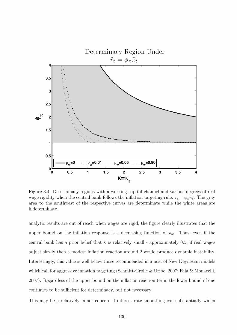
0 0.5 1 1.5 2 2.5 3 3.5 40

0.5

1

1.5

2

2.5

3

3.5

4

κ=κr

φ π

Determinacy Region Underrt = φππt

ρw

=0 ρw

=0.01 ρw

=0.05 ρw

=0.90

Figure 3.4: Determinacy regions with a working capital channel and various degrees of realwage rigidity when the central bank follows the inflation targeting rule: rt = φππt. The grayarea to the southwest of the respective curves are determinate while the white areas areindeterminate.

analytic results are out of reach when wages are rigid, the figure clearly illustrates that the

upper bound on the inflation response is a decreasing function of ρw. Thus, even if the

central bank has a prior belief that κ is relatively small - approximately 0.5, if real wages

adjust slowly then a modest inflation reaction around 2 would produce dynamic instability.

Interestingly, this value is well below those recommended in a host of New-Keynesian models

which call for aggressive inflation targeting (Schmitt-Grohe & Uribe, 2007; Faia & Monacelli,

2007). Regardless of the upper bound on the inflation reaction term, the lower bound of one

continues to be sufficient for determinacy, but not necessary.

This may be a relatively minor concern if interest rate smoothing can substantially widen

130

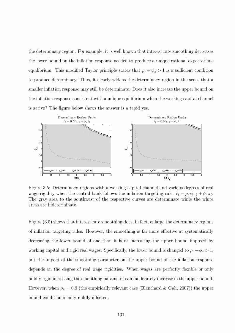
the determinacy region. For example, it is well known that interest rate smoothing decreases

the lower bound on the inflation response needed to produce a unique rational expectations

equilibrium. This modified Taylor principle states that ρr +φπ > 1 is a sufficient condition

to produce determinacy. Thus, it clearly widens the determinacy region in the sense that a

smaller inflation response may still be determinate. Does it also increase the upper bound on

the inflation response consistent with a unique equilibrium when the working capital channel

is active? The figure below shows the answer is a tepid yes.

0 0.5 1 1.5 2 2.5 3 3.5 40

0.5

1

1.5

2

2.5

3

3.5

4

κ=κr

φ π

Determinacy Region Underrt = 0.5rt−1 + φππt

ρw

=0 ρw

=0.01 ρw

=0.05 ρw

=0.90

0 0.5 1 1.5 2 2.5 3 3.5 40

0.5

1

1.5

2

2.5

3

3.5

4

κ=κr

φ π

Determinacy Region Underrt = 0.8rt−1 + φππt

ρw

=0 ρw

=0.01 ρw

=0.05 ρw

=0.90

Figure 3.5: Determinacy regions with a working capital channel and various degrees of realwage rigidity when the central bank follows the inflation targeting rule: rt = ρrrt−1 +φππt.The gray area to the southwest of the respective curves are determinate while the whiteareas are indeterminate.

Figure (3.5) shows that interest rate smoothing does, in fact, enlarge the determinacy regions

of inflation targeting rules. However, the smoothing is far more effective at systematically

decreasing the lower bound of one than it is at increasing the upper bound imposed by

working capital and rigid real wages. Specifically, the lower bound is changed to ρr+φπ > 1,

but the impact of the smoothing parameter on the upper bound of the inflation response

depends on the degree of real wage rigidities. When wages are perfectly flexible or only

mildly rigid increasing the smoothing parameter can moderately increase in the upper bound.

However, when ρw = 0.9 (the empirically relevant case (Blanchard & Gali, 2007)) the upper

bound condition is only mildly affected.

131

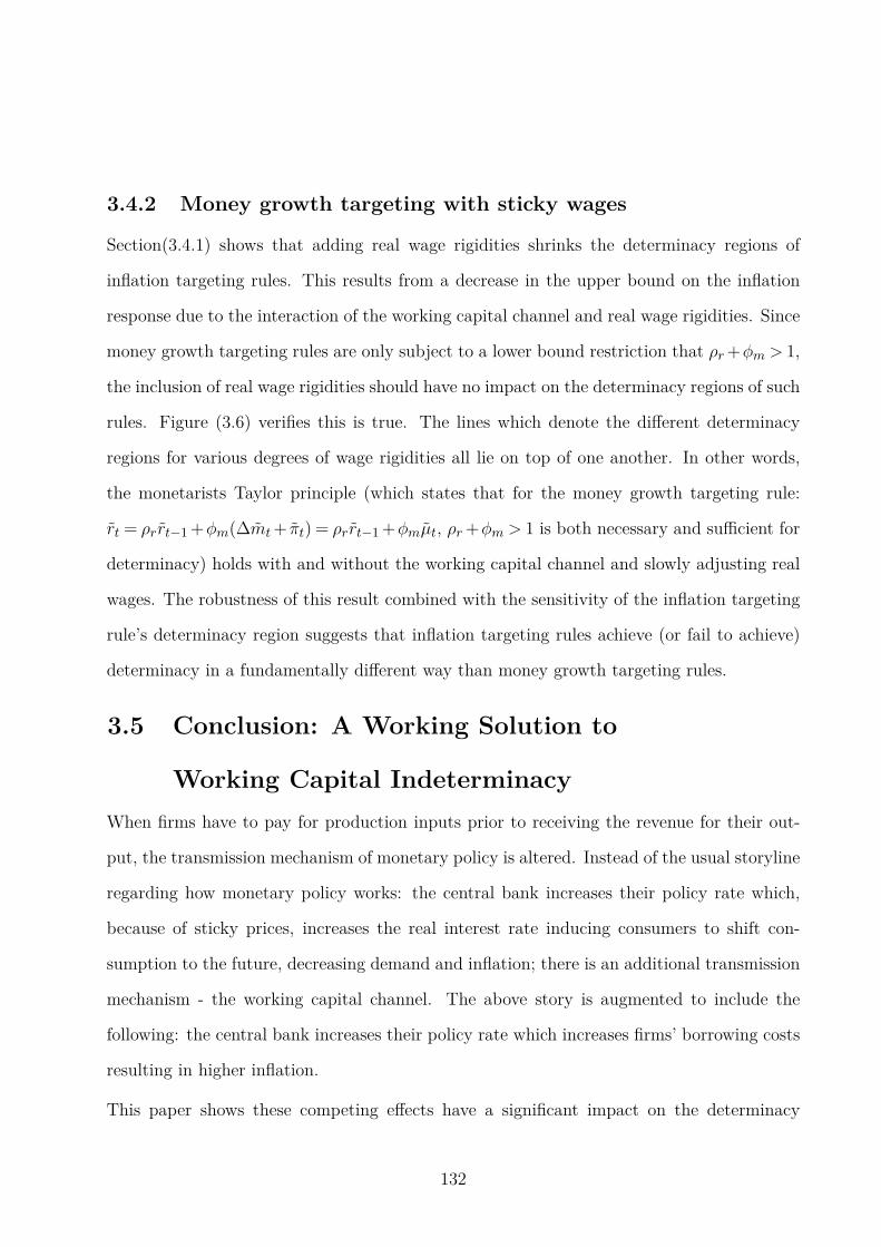
3.4.2 Money growth targeting with sticky wages

Section(3.4.1) shows that adding real wage rigidities shrinks the determinacy regions of

inflation targeting rules. This results from a decrease in the upper bound on the inflation

response due to the interaction of the working capital channel and real wage rigidities. Since

money growth targeting rules are only subject to a lower bound restriction that ρr+φm > 1,

the inclusion of real wage rigidities should have no impact on the determinacy regions of such

rules. Figure (3.6) verifies this is true. The lines which denote the different determinacy

regions for various degrees of wage rigidities all lie on top of one another. In other words,

the monetarists Taylor principle (which states that for the money growth targeting rule:

rt = ρrrt−1 +φm(∆mt+ πt) = ρrrt−1 +φmµt, ρr+φm > 1 is both necessary and sufficient for

determinacy) holds with and without the working capital channel and slowly adjusting real

wages. The robustness of this result combined with the sensitivity of the inflation targeting

rule’s determinacy region suggests that inflation targeting rules achieve (or fail to achieve)

determinacy in a fundamentally different way than money growth targeting rules.

3.5 Conclusion: A Working Solution to

Working Capital Indeterminacy

When firms have to pay for production inputs prior to receiving the revenue for their out-

put, the transmission mechanism of monetary policy is altered. Instead of the usual storyline

regarding how monetary policy works: the central bank increases their policy rate which,

because of sticky prices, increases the real interest rate inducing consumers to shift con-

sumption to the future, decreasing demand and inflation; there is an additional transmission

mechanism - the working capital channel. The above story is augmented to include the

following: the central bank increases their policy rate which increases firms’ borrowing costs

resulting in higher inflation.

This paper shows these competing effects have a significant impact on the determinacy

132

0 0.5 1 1.5 2 2.5 3 3.5 40

0.5

1

1.5

2

2.5

3

3.5

4

κ=κr

φ m

Determinacy Region Underrt = φm(∆mt + πt)

ρw

=0 ρw

=0.01 ρw

=0.05 ρw

=0.90

Figure 3.6: Determinacy regions with a working capital channel and various degrees of realwage rigidity when the central bank follows the inflation targeting rule: rt = φm(∆mt+ πt).The gray area to the southwest of the respective curves are determinate while the whiteareas are indeterminate.

regions of inflation targeting rules. Most notably, strict inflation targeting is especially

susceptible to indeterminacy. The more common form of inflation targeting whereby the

central bank adjusts its policy rate to achieve their inflation objective is also vulnerable to

working capital indeterminacy. Typically, such rules are only subject to the well known lower

bound of one on the inflation objective known as the Taylor principle. However, when the

working capital channel is active, the inflation response is also subject to an upper bound.

The exact value depends on the slope of the Phillips curve and the degree of real wage

rigidity and lesser so on the degree of inertia in the policy rule.

What is perhaps more surprising than the sensitivity of the inflation targeting rule’s deter-

133

minacy region is the robustness of the determinacy region of money growth targeting rules.

Whether the central bank chooses to fully stabilize the growth rate of nominal money such

as Friedman (1960) suggested when proposing his k-percent rule, or they simply adjust their

policy rate to achieve their money growth objective the determinacy regions are large and

stable. Specifically, for flexible money growth targeting rules rt = ρrrt−1 +φm(∆mt + πt)

the simple condition that ρr +φm > 1 is both necessary and sufficient for the existence of a

unique rational expectations equilibrium across models with and without the working capital

channel and sticky real wages.

Given the fact that aggressive inflation targeting is typically considered optimal from a nor-

mative standpoint (Schmitt-Grohe & Uribe, 2007; Faia & Monacelli, 2007), the inability of

this rule to bring about a unique rational expectations equilibrium poses a serious hurdle

to implementing inflation targeting. The ability of money growth targeting to anchor ex-

pectations on a unique equilibrium offers one solution to this problem: Augment the typical

inflation targeting interest rate rule with a money growth response. Figure (3.7) shows that

a relatively modest focus on money growth can greatly widen the determinacy regions of in-

flation targeting rules. Unlike interest rate smoothing, the money growth response enlarges

the determinacy region even for large degrees of real wage rigidity.

Although the money growth response stabilizes the determinacy region of inflation targeting

rules across working capital and sticky wage models, the question of whether this response

is optimal still remains. In particular, there is a long standing literature which argues that

reacting to money exposes the economy to the additional volatility of money demand shocks

(Poole, 1970). Thus, money growth targeting is typically thought to be inferior to inflation

targeting (Gali, 2008). However, the inability of inflation targeting rules to pin down a

unique equilibrium may pose a trade-off for policy makers.

Future work should explore the details of this trade-off. By anchoring expectations, some

degree of money growth targeting may be optimal since it enables the central bank to more

aggressively target inflation. However, this is likely an empirical question, as the degree

134

0 0.5 1 1.5 2 2.5 3 3.5 40

0.5

1

1.5

2

2.5

3

3.5

4

κ=κr

φ π

Determinacy Region Underrt = 1.5(∆mt + πt) + φππt

ρw

=0 ρw

=0.01 ρw

=0.05 ρw

=0.90

Figure 3.7: Determinacy regions with a working capital channel and various degrees of realwage rigidity when the central bank follows the inflation targeting rule: rt = 1.5(∆mt+ πt)+φππt. The gray area is determinate.

of money growth targeting that is optimal depends on the slope of the Phillips curve, the

degree of real wage rigidities and the relative sizes of the standard deviation of money demand

disturbances to drivers of the business cycle. The survey by Schorfheide (2008) suggests there

may be a wide range of estimates of the slope parameter. Given this parameter uncertainty, a

useful exercise would be to analyze robustly optimal monetary policy in this working capital

augmented New-Keynesian model as in Giannoni (2002).

135

References

Anderson, R. G. & Jones, B. (2011). A comprehensive revision of the U.S. monetary services

(divisia) indexes. Review, (Sep), 325–360.

Barnett, W., Liu, J., Mattson, R., & Noort, J. (2013). The New CFS Divisia Monetary

Aggregates: Design, Construction, and Data Sources. Open Economies Review, 24(1),

101–124.

Barnett, W. A. (1978). The user cost of money. Economics Letters, 1(2), 145–149.

Barnett, W. A. (1980). Economic monetary aggregates an application of index number and

aggregation theory. Journal of Econometrics, 14(1), 11–48.

Belongia, M. T. & Ireland, P. N. (2014). The barnett critique after three decades: A new

keynesian analysis. Journal of Econometrics, forthcoming.

Blanchard, O. & Gali, J. (2007). Real Wage Rigidities and the New Keynesian Model.

Journal of Money, Credit and Banking, 39(s1), 35–65.

Christiano, L. J., Eichenbaum, M., & Evans, C. L. (2005). Nominal Rigidities and the

Dynamic Effects of a Shock to Monetary Policy. Journal of Political Economy, 113(1),

1–45.

Christiano, L. J., Trabandt, M., & Walentin, K. (2010). DSGE Models for Monetary Policy

Analysis. In B. M. Friedman & M. Woodford (Eds.), Handbook of Monetary Economics,

volume 3 of Handbook of Monetary Economics chapter 7, (pp. 285–367). Elsevier.

136

Coibion, O. & Gorodnichenko, Y. (2011). Monetary Policy, Trend Inflation, and the Great

Moderation: An Alternative Interpretation. American Economic Review, 101(1), 341–70.

Curdia, V. & Woodford, M. (2010). Credit spreads and monetary policy. Journal of Money,

Credit and Banking, 42(s1), 3–35.

Diewert, W. E. (1976). Exact and superlative index numbers. Journal of Econometrics,

4(2), 115–145.

Faia, E. & Monacelli, T. (2007). Optimal interest rate rules, asset prices, and credit frictions.

Journal of Economic Dynamics and Control, 31(10), 3228–3254.

Friedman, M. (1960). A Program for Monetary Stability. Fordham University Press.

Friedman, M. & Schwartz, A. J. (1971). A Monetary History of the United States, 1867-1960.

Princeton University Press.

Gali, J. (2008). Monetary Policy, Inflation, and the Business Cycle: An Introduction to the

New Keynesian Framework. Princeton University Press.

Giannoni, M. P. (2002). Does model uncertainty justify caution? robust optimal monetary

policy in a forward-looking model. Macroeconomic Dynamics, 6(01), 111–144.

Ireland, P. N. (2009). On the welfare cost of inflation and the recent behavior of money

demand. American Economic Review, 99(3), 1040–52.

Kahn, G. A. & Benolkin, S. (2007). The role of money in monetary policy: why do the Fed

and ECB see it so differently? Economic Review, (Q III), 5–36.

Keating, J. W. & Smith, A. L. (2013). Determinacy and Indeterminacy in Monetary Policy

Rules with Money. WORKING PAPERS SERIES IN THEORETICAL AND APPLIED

ECONOMICS 201310, University of Kansas, Department of Economics.

137

McCallum, B. T. (1998). Solutions to linear rational expectations models: a compact expo-

sition. Economics Letters, 61(2), 143–147.

Mishkin, F. (2013). The Economics Of Money, Banking And Financial Markets. Pearson.

Poole, W. (1970). Optimal choice of monetary policy instruments in a simple stochastic

macro model. The Quarterly Journal of Economics, 84(2), 197–216.

Roger, S. (2010). Inflation targeting turns 20. Finance & Development, 47(1), 46–49.

Rotemberg, J. J. (1982). Sticky prices in the united states. Journal of Political Economy,

90(6), 1187–1211.

Schmitt-Grohe, S. & Uribe, M. (2007). Optimal simple and implementable monetary and

fiscal rules. Journal of Monetary Economics, 54(6), 1702–1725.

Schorfheide, F. (2008). Dsge model-based estimation of the new keynesian phillips curve.

FRB Richmond Economic Quarterly, 94(4), 397–433.

Sims, C. A. (1992). Interpreting the macroeconomic time series facts : The effects of mone-

tary policy. European Economic Review, 36(5), 975–1000.

Smets, F. & Wouters, R. (2007). Shocks and Frictions in US Business Cycles: A Bayesian

DSGE Approach. American Economic Review, 97(3), 586–606.

Svensson, L. E. O. (1999). Inflation targeting as a monetary policy rule. Journal of Monetary

Economics, 43(3), 607–654.

Taylor, J. B. (1993). Discretion versus policy rules in practice. Carnegie-Rochester Confer-

ence Series on Public Policy, 39(1), 195–214.

Taylor, J. B. (1999). Staggered price and wage setting in macroeconomics. In J. B. Taylor

& M. Woodford (Eds.), Handbook of Macroeconomics, volume 1 of Handbook of Macroe-

conomics chapter 15, (pp. 1009–1050). Elsevier.

138

Thornton, D. L. (2012). Greenspan’s conundrum and the Fed’s ability to affect long-term

yields. Federal reserve bank of st. louis, working papers, Federal Reserve Bank of St.

Louis.

Woodford, M. (1999). Commentary : how should monetary policy be conducted in an era of

price stability? Proceedings - Economic Policy Symposium - Jackson Hole, (pp. 277–316).

139

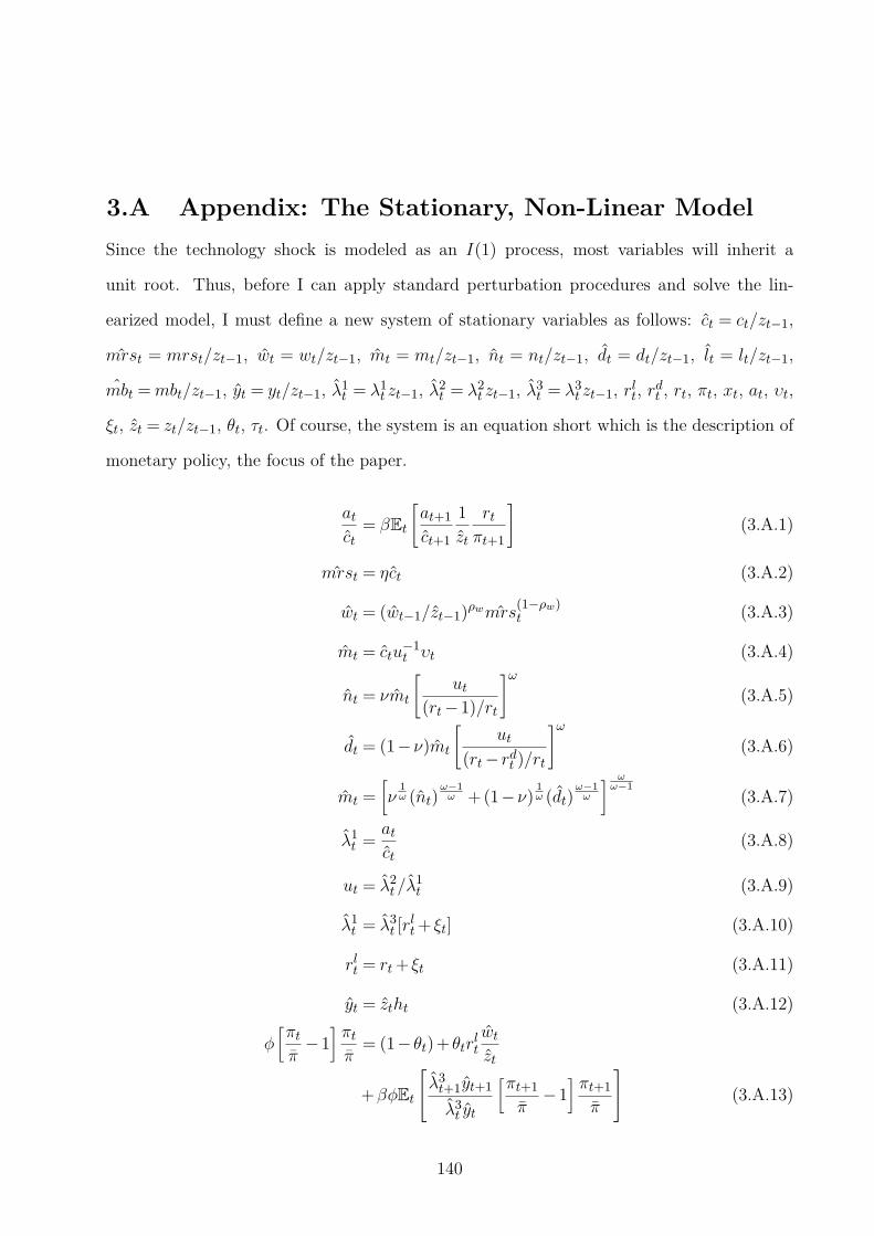
3.A Appendix: The Stationary, Non-Linear Model

Since the technology shock is modeled as an I(1) process, most variables will inherit a

unit root. Thus, before I can apply standard perturbation procedures and solve the lin-

earized model, I must define a new system of stationary variables as follows: ct = ct/zt−1,

mrst = mrst/zt−1, wt = wt/zt−1, mt = mt/zt−1, nt = nt/zt−1, dt = dt/zt−1, lt = lt/zt−1,

mbt =mbt/zt−1, yt = yt/zt−1, λ1t = λ1

t zt−1, λ2t = λ2

t zt−1, λ3t = λ3

t zt−1, rlt, rdt , rt, πt, xt, at, υt,

ξt, zt = zt/zt−1, θt, τt. Of course, the system is an equation short which is the description of

monetary policy, the focus of the paper.

atct

= βEt

[

at+1

ct+1

1

zt

rtπt+1

]

(3.A.1)

mrst = ηct (3.A.2)

wt = (wt−1/zt−1)ρwmrs(1−ρw)t (3.A.3)

mt = ctu−1t υt (3.A.4)

nt = νmt

[

ut(rt−1)/rt

]ω

(3.A.5)

dt = (1−ν)mt

[

ut

(rt− rdt )/rt

]ω

(3.A.6)

mt =[

ν1ω (nt)

ω−1ω +(1−ν)

1ω (dt)

ω−1ω

] ωω−1

(3.A.7)

λ1t =

atct

(3.A.8)

ut = λ2t /λ

1t (3.A.9)

λ1t = λ3

t [rlt+ ξt] (3.A.10)

rlt = rt+ ξt (3.A.11)

yt = ztht (3.A.12)

φ[πtπ

−1]πtπ

= (1− θt)+ θtrltwtzt

+βφEt

λ3t+1yt+1

λ3t yt

[πt+1

π−1

]πt+1

π

(3.A.13)

140

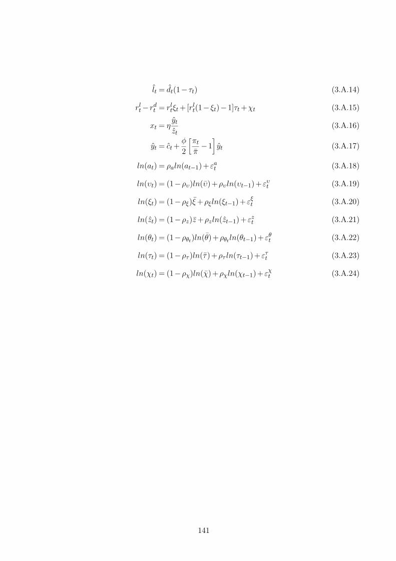
lt = dt(1− τt) (3.A.14)

rlt− rdt = rltξt+[rlt(1− ξt)−1]τt+χt (3.A.15)

xt = ηytzt

(3.A.16)

yt = ct+φ

2

[πtπ

−1]

yt (3.A.17)

ln(at) = ρaln(at−1)+ εat (3.A.18)

ln(υt) = (1−ρυ)ln(υ)+ρυln(υt−1)+ ευt (3.A.19)

ln(ξt) = (1−ρξ)ξ+ρξln(ξt−1)+ εξt (3.A.20)

ln(zt) = (1−ρz)z+ρzln(zt−1)+ εzt (3.A.21)

ln(θt) = (1−ρθt)ln(θ)+ρθt

ln(θt−1)+ εθt (3.A.22)

ln(τt) = (1−ρτ )ln(τ)+ρτ ln(τt−1)+ ετt (3.A.23)

ln(χt) = (1−ρχ)ln(χ)+ρχln(χt−1)+ εχt (3.A.24)

141

3.B Appendix: Proofs

In this section I present the proofs to our results stated in the paper. All proofs for de-

terminacy omit the possibility that an eigenvalue is exactly equal to one. In such a case,

a log-linear approximation to the non-linear model can not pin down the question of local

existence and uniqueness.

Proposition 3.1

Consider the dynamic system defined by equations (3.1), (3.2) and (3.4),

AEt[wt+1] =Bwt+Cst.

A=

1 1 −1

0 β κr

0 0 0

B =

1 0 0

−κ 1 0

0 −1 0

where wt =

[

xt, πt, rt−1

]T

and C is a conformable matrix for the vector

st =

[

at, zt, ξt, θt

]T

. The system has two non-predetermined variables and one prede-

termined variable. Therefore, the system will have a unique rational expectations equilibrium

(REE) if, and only if, two roots λ which satisfy |B−λA |= 0 lie outside the unit circle and

remaining two roots lie inside the unit circle McCallum (1998). The generalized eigenvalues

142

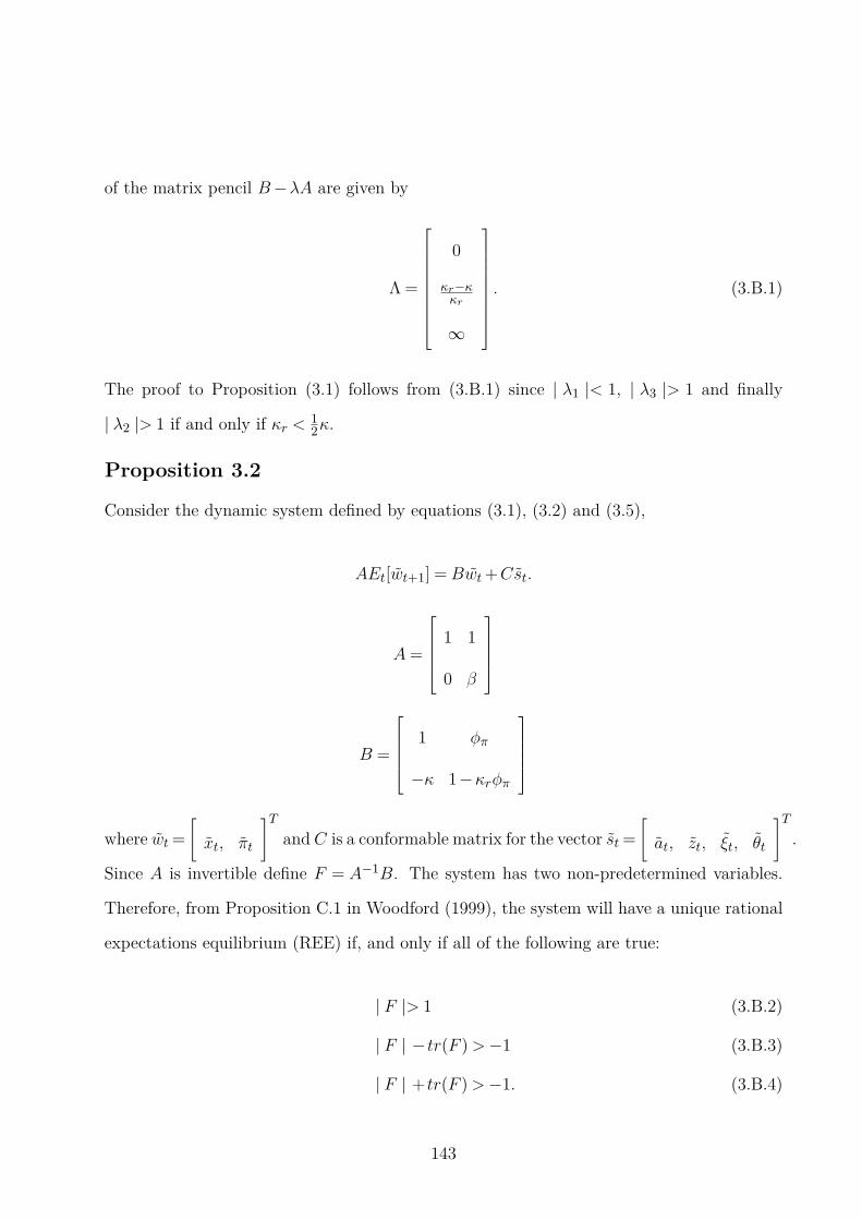
of the matrix pencil B−λA are given by

Λ =

0

κr−κκr

∞

. (3.B.1)

The proof to Proposition (3.1) follows from (3.B.1) since | λ1 |< 1, | λ3 |> 1 and finally

| λ2 |> 1 if and only if κr <12κ.

Proposition 3.2

Consider the dynamic system defined by equations (3.1), (3.2) and (3.5),

AEt[wt+1] =Bwt+Cst.

A=

1 1

0 β

B =

1 φπ

−κ 1−κrφπ

where wt =

[

xt, πt

]T

and C is a conformable matrix for the vector st =

[

at, zt, ξt, θt

]T

.

Since A is invertible define F = A−1B. The system has two non-predetermined variables.

Therefore, from Proposition C.1 in Woodford (1999), the system will have a unique rational

expectations equilibrium (REE) if, and only if all of the following are true:

| F |> 1 (3.B.2)

| F | − tr(F )>−1 (3.B.3)

| F | + tr(F )>−1. (3.B.4)

143

Since κ ≥ κr, let κr = ακ where α ∈ [0,1]. First notice that (3.B.2) is satisfied, | F |=1+κφπ(1−α)

β > 1. Moreover, since tr(F ) = 1+κ(1−αφπ)ββ , it follows that

| F | − tr(F ) =κ(φπ −1)−β

β>−1 ⇐⇒ κ(φπ −1)> 0 ⇐⇒ φπ > 1.

Finally, for the condition in (3.B.4) to be satisfied, we must have:

| F | + tr(F ) =2+κ+β+φπκ(1−2α)

β>−1 ⇐⇒ 2(1+β)+κ+φπκ(1−2α)> 0.

Rearranging the last inequality, the condition from Proposition (3.2) emerges:

φπ <

∞ if α≤ 12

2(1+β)+κκ(2α−1) if α > 1

2 .

Proposition 3.3

The dynamic system consisting of (3.1), (3.2), (3.3) and (3.7) can be expressed as

AEt[wt+1] =Bwt+Cst.

A=

1 1 −1 0

0 β κr 0

0 0 0 1

0 0 ηr 1

144

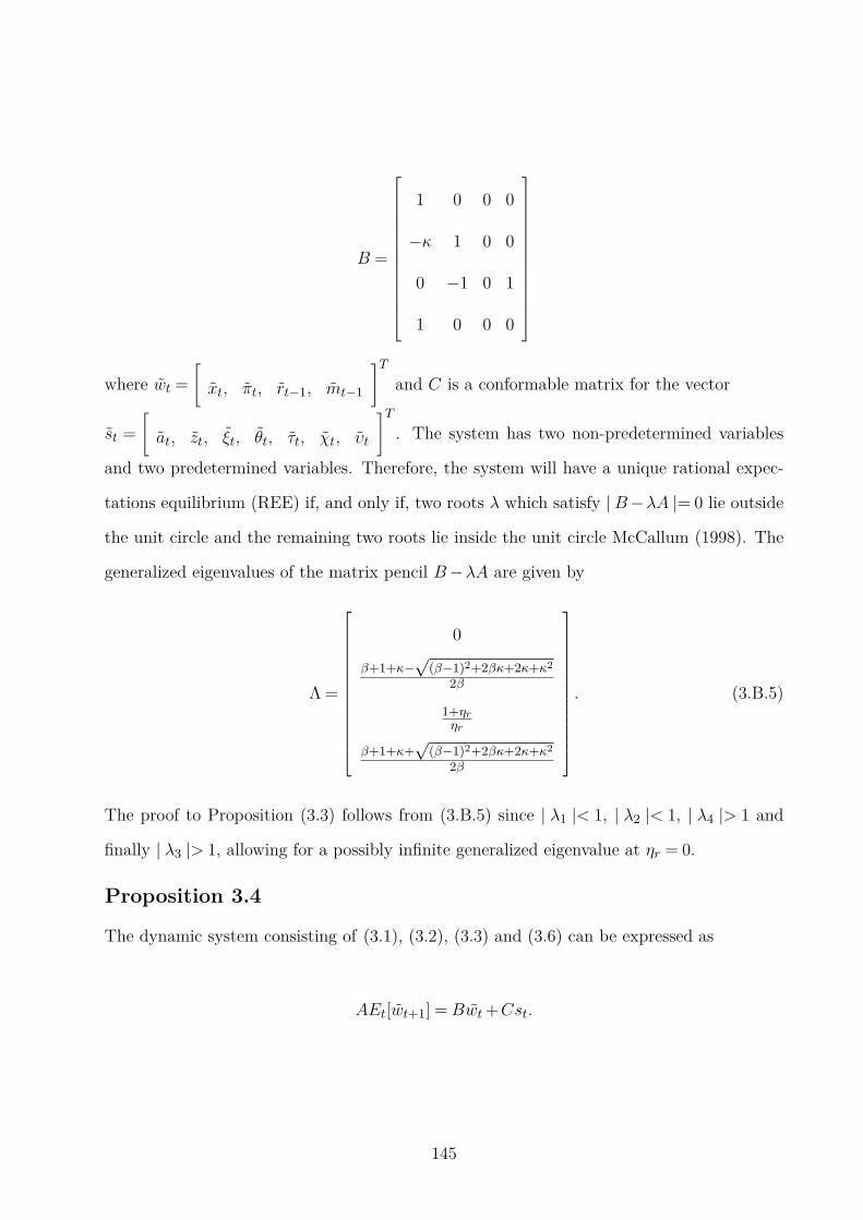
B =

1 0 0 0

−κ 1 0 0

0 −1 0 1

1 0 0 0

where wt =

[

xt, πt, rt−1, mt−1

]T

and C is a conformable matrix for the vector

st =

[

at, zt, ξt, θt, τt, χt, υt

]T

. The system has two non-predetermined variables

and two predetermined variables. Therefore, the system will have a unique rational expec-

tations equilibrium (REE) if, and only if, two roots λ which satisfy |B−λA |= 0 lie outside

the unit circle and the remaining two roots lie inside the unit circle McCallum (1998). The

generalized eigenvalues of the matrix pencil B−λA are given by

Λ =

0

β+1+κ−√

(β−1)2+2βκ+2κ+κ2

2β

1+ηr

ηr

β+1+κ+√

(β−1)2+2βκ+2κ+κ2

2β

. (3.B.5)

The proof to Proposition (3.3) follows from (3.B.5) since | λ1 |< 1, | λ2 |< 1, | λ4 |> 1 and

finally | λ3 |> 1, allowing for a possibly infinite generalized eigenvalue at ηr = 0.

Proposition 3.4

The dynamic system consisting of (3.1), (3.2), (3.3) and (3.6) can be expressed as

AEt[wt+1] =Bwt+Cst.

145

A=

1 1 −1 0

0 β κr 0

0 0 1 −φm

0 0 ηr 1

B =

1 0 0 0

−κ 1 0 0

0 φm ρr −φm

1 0 0 0

where wt =

[

xt, πt, rt−1, mt−1

]T

and C is a conformable matrix for the vector

st =

[

at, zt, ξt, θt, τt, χt, υt

]T

. The system has two non-predetermined variables

and two predetermined variables. Therefore, the system will have a unique rational expec-

tations equilibrium (REE) if, and only if, two roots λ which satisfy |B−λA |= 0 lie outside

the unit circle and the remaining two roots lie inside the unit circle McCallum (1998). The

generalized eigenvalues of the matrix pencil B−λA are given by

Λ =

0

β+1+κ−√

(β−1)2+2βκ+2κ+κ2

2β

ρr+φm+ηrφm

1+ηrφm

β+1+κ+√

(β−1)2+2βκ+2κ+κ2

2β

. (3.B.6)

The proof to Proposition (3.4) follows from (3.B.6) since | λ1 |< 1, | λ2 |< 1, | λ4 |> 1 and

finally | λ3 |> 1 if, and only if, ρr +φm > 1.

146

Lemma 3.1

Before deriving the final a result, a few useful observations will allow for a simpler proof.

First, define the user costs of nt and dt respectively by:

unt =rt−1

rt(3.B.7)

udt =rt− rdtrt

. (3.B.8)

These expressions appear from the first order conditions for currency and deposits; in par-

ticular,∂ut∂nt

∂ut∂dt

=∂ut∂mt

∂mt∂nt

∂ut∂mt

∂mt∂dt

=rt−1rt

rt−rdt

rt

≡ untudt,

where the last equality uses the representative household’s first order conditions (5.10) and

(3.12). Using these definitions of the user-cost of monetary assets, combine (5.10) and (3.12)

to eliminate nt and dt from (3.6). Solving the resulting expression for λ2t /λ

1t and define the

resulting expression as:

λ2t

λ1t

= ut =[

ν(unt )1−ω +(1−ν)(udt )1−ω

] 11−ω , (3.B.9)

the user-cost of the entire monetary aggregate. Finally, notice that given the definitions

of (3.B.7), (3.B.8) and (3.B.9), ut satisfies Irving Fisher’s factor reversal test which mathe-

matically states that total expenditures on monetary assets must equal the product of the

quantity and price aggregate:

unt nt+udt dt =mtuωt

[

ν(unt )1−ω +(1−ν)(udt )1−ω

]

=mtut. (3.B.10)

This expression will prove very useful in the following proof. From Definition (3.1), we have

147

the growth rate of the Divisia monetary aggregate is given by

ln(µt) =

(

snt + snt−1

2

)

ln

(

ntnt−1

)

+

(

sdt + sdt−1

2

)

ln

(

dtdt−1

)

+ ln(πt).

Now substituting the factor demands ((5.10) and (3.12)) into the definition of the Divisia

monetary aggregate to eliminate nt and dt, we obtain the following useful expression for the

difference between the growth rates of the Divisia monetary aggregate and the true monetary

aggregate:

ln(µt)−∆ln(mt)− ln(πt) = ω[

∆ln(

ut(unt ,u

dt ))]

−ω[1

2

(

snt + snt−1

)

∆ln(unt )− 1

2

(

sdt + sdt−1

)

∆ln(

udt)]

≡ E(ln(unt ), ln(udt ), ln(unt−1), ln(udt−1)),

where E is the error-term which quantifies the difference between the Divisia monetary

aggregate and the true monetary aggregate. This expression is a function only of user-costs

and completely independent of the quantities of monetary assets. This can easily be seen

since the denominator of the expenditure share weights snt and sdt is total expenditures which

depends only on ut and mt from (3.B.10):

snt =unt nt

unt nt+unt nt=mtu

ωt ν(unt )1−ω

utmt= ν

(

untut

)1−ω

sdt =udt dt

unt nt+unt nt=mtu

ωt (1−ν)(udt )

1−ω

utmt= (1−ν)

(

udtut

)1−ω

.

To verify the claim, take a first-order Taylor approximation of E around the steady state,

hence all derivatives below are evaluated at the steady state. For this reason, all derivatives

with respect to the share weights sn(unt ,udt ) and sd(unt ,u

dt ) evaluate to zero since in steady

148

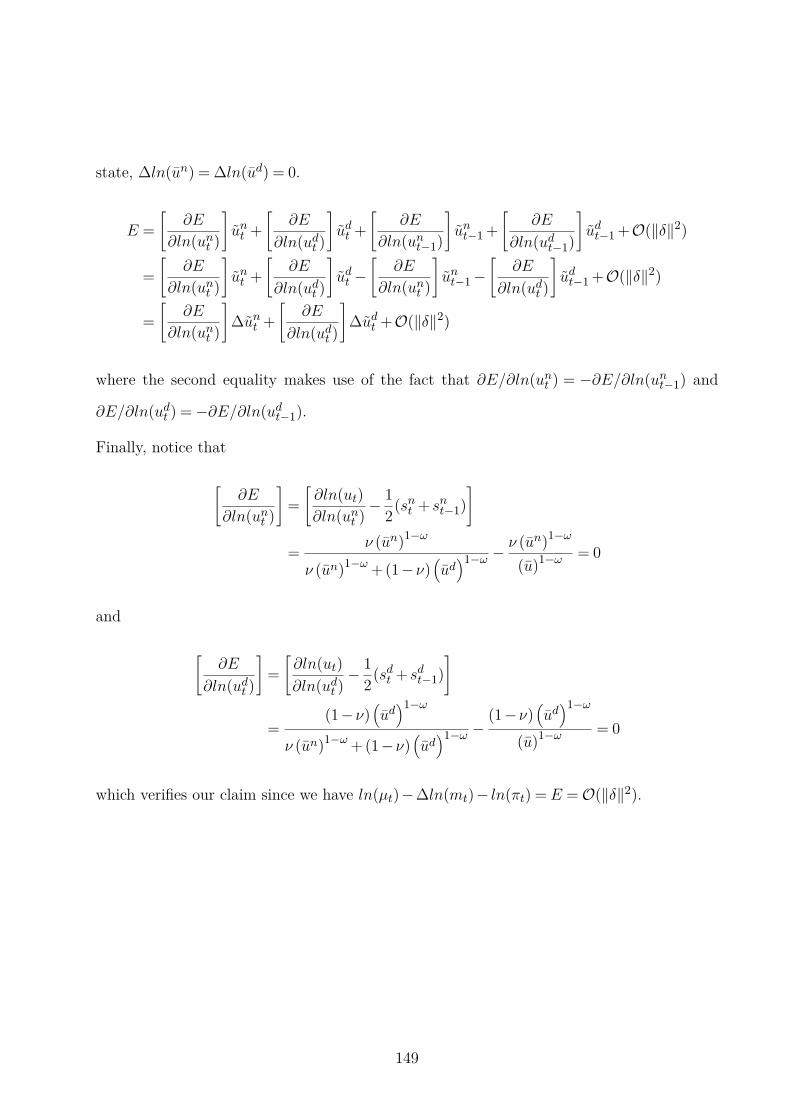
state, ∆ln(un) = ∆ln(ud) = 0.

E =

[

∂E

∂ln(unt )

]

unt +

[

∂E

∂ln(udt )

]

udt +

[

∂E

∂ln(unt−1)

]

unt−1 +

[

∂E

∂ln(udt−1)

]

udt−1 +O(‖δ‖2)

=

[

∂E

∂ln(unt )

]

unt +

[

∂E

∂ln(udt )

]

udt −[

∂E

∂ln(unt )

]

unt−1 −[

∂E

∂ln(udt )

]

udt−1 +O(‖δ‖2)

=

[

∂E

∂ln(unt )

]

∆unt +

[

∂E

∂ln(udt )

]

∆udt +O(‖δ‖2)

where the second equality makes use of the fact that ∂E/∂ln(unt ) = −∂E/∂ln(unt−1) and

∂E/∂ln(udt ) = −∂E/∂ln(udt−1).

Finally, notice that

[

∂E

∂ln(unt )

]

=

[

∂ln(ut)

∂ln(unt )− 1

2(snt + snt−1)

]

=ν (un)1−ω

ν (un)1−ω +(1−ν)(

ud)1−ω − ν (un)1−ω

(u)1−ω = 0

and

[

∂E

∂ln(udt )

]

=

[

∂ln(ut)

∂ln(udt )− 1

2(sdt + sdt−1)

]

=(1−ν)

(

ud)1−ω

ν (un)1−ω +(1−ν)(

ud)1−ω −

(1−ν)(

ud)1−ω

(u)1−ω = 0

which verifies our claim since we have ln(µt)−∆ln(mt)− ln(πt) = E = O(‖δ‖2).

149

Chapter 4

House Prices, Heterogeneous Banks

and Unconventional Monetary Policy

Options

4.1 Introduction

The first drop in U.S. home prices since the Great Depression resulted in the 2008 Financial

Crisis, forcing policy makers to ‘Fly Blind,’ and take the exceptional actions of injecting

equity into the largest U.S. financial firms and making a myriad of asset purchases without

a playbook from economists. Little was known regarding the exact financial mechanisms

linking home prices to the rest of the economy, and to date, many questions remain. Why

did a drop in home prices set off a financial panic that forced the largest commercial banks

to shed relatively more assets than their smaller counter-parts? What is the transmission

mechanism of equity injections into these big banks and large-scale asset purchases amidst

a housing-centered credit crunch?

In this paper, I propose an empirically motivated financial mechanism which provides an

answer to both of these questions. I embed this financial structure into an otherwise stan-

150

dard Real Business Cycle model to illustrate its ability to generate salient features of the

U.S. economy. Quantitatively, the model matches empirical correlations that the traditional

financial accelerator mechanism (Bernanke et al., 1999) (BGG) fails to capture, including

the correlation of finance premiums with home prices, investment and output. I then test

the model’s qualitative predictions against an estimated VAR. The results of these empirical

comparisons support the model’s financial structure.

I am not alone in my efforts to adapt existing financial accelerator frameworks to simulate

the effects of unconventional monetary policy in light of the financial crisis. However, these

models typically rely on ‘Financial” shocks to generate a crisis scenario and quadratic in-

vestment adjustment costs to propagate the downturn (Gertler & Karadi, 2011). In such

models, no distinction is made between housing secured debt and other assets.

I take the alternative viewpoint that housing, and housing secured debt instruments, played

a particularly important role in the crisis. In particular, the housing and financial sector in

the model I develop are highly integrated – a feature that allows for a financial crunch to

originate from a change in primitives such as preferences over housing. Moreover, the use of

housing as an ultimate source of collateral for financial assets provides a natural source to

propagate downturns as opposed to quadratic investment adjustment costs. Upon default,

the liquidation of housing – a durable – increases the stock of homes and therefore decreases

prices into the future. Furthermore, the time lag between default and liquidation leads

to hump-shaped impulse response functions of output, an empirical feature used to justify

quadratic adjustment costs (cf Christiano et al. (2005)).

Besides treating the housing and the financial sector as independent, other models that have

been used to analyze unconventional monetary policy fail to provide an answer regarding

the effects, and desirability, of equity injections into “Too Big to Fail” banks. These papers

assume either: (i) All banks are the same in terms of size and efficiency (Gertler & Kiyotaki,

2010) or (ii) Banks differ in terms of size and efficiency, but banks face no agency problems

(Hafstead & Smith, 2012).

151

However, both of these assumption are at odds with the empirical evidence. Recent estimates

of scale efficiency in the financial sector, including off-balance sheet activities, have found

that “Bigger is Better” (Wheelock & Wilson, 2012; Bos & Kolari, 2013). As for the later

assumption, Demirguc-Kunt et al. (2013) find that bank capital is an important determinant

for the performance of banks, most markedly for big banks – empirical support for over-

turning the Modigliani-Miller theorem.1

With this empirical evidence in mind, I incorporate bank heterogeneity into the financial

sector. Big banks naturally arise in equilibrium due to their superior efficiency intermediating

housing-secured assets, relative to small banks. The only question is: Why do small banks

operate at all in this market if they are technologically dis-advantaged? This is where

eschewing the assumption that banks face no agency problems is key. The big/productive

banks in the model face a moral-hazard problem. Therefore, the amount of housing-secured

assets the productive bank can hold is determined by its capital. In this sense, bank-capital

is key for the operation of big/productive banks, consistent with the empirical evidence.

By capturing the rich interaction between the housing market and the heterogeneous financial

sector, the model is able to offer an explanation as to why the concentration of assets in the

biggest commercial banks decreased with home prices, as illustrated below.

The financial mechanism I propose is capable of endogenously generating the above co-

movement. Beyond simply capturing a correlation, the model provides the insight that the

above redistribution increased the severity and length of the Great Recession. However,

the same feedback mechanism provides traction for equity injections into big banks and

large-scale asset purchase programs.

1The Modigliani-Miller theorem states that how a firm chooses to fund itself (debt vs. equity) is irrelevant.

152

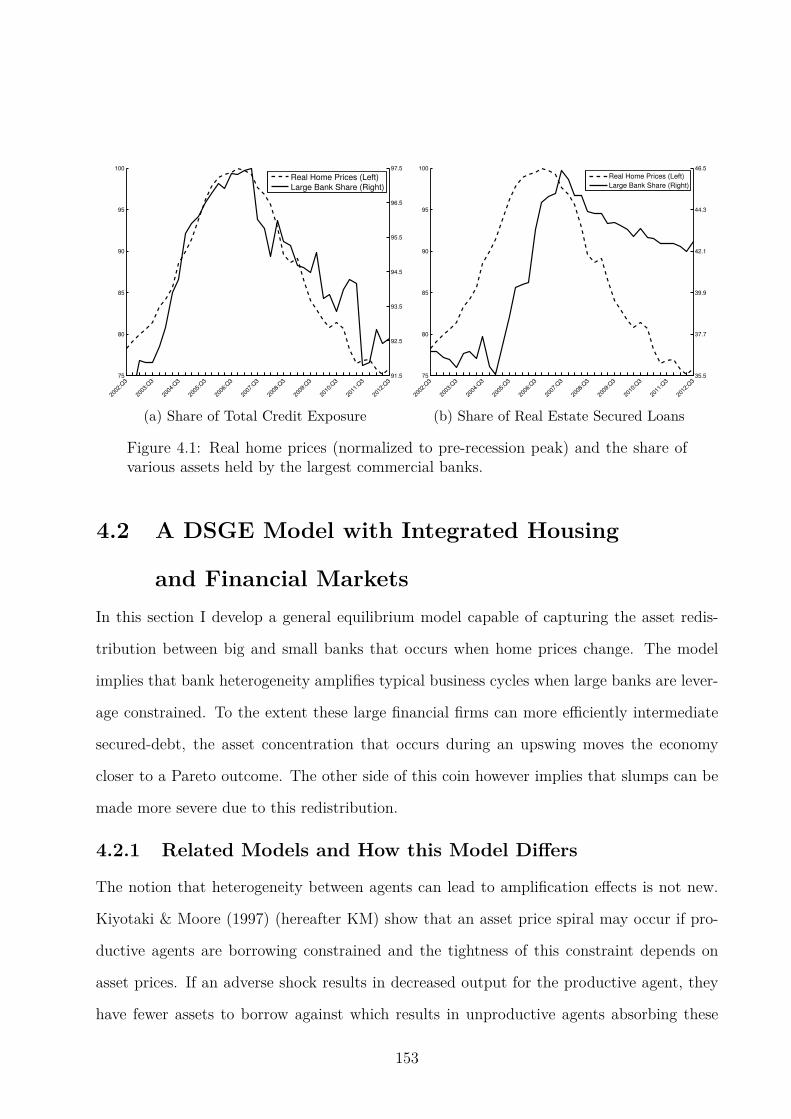
75

80

85

90

95

100

2002

:Q3

2003

:Q3

2004

:Q3

2005

:Q3

2006

:Q3

2007

:Q3

2008

:Q3

2009

:Q3

2010

:Q3

2011

:Q3

2012

:Q3

91.5

92.5

93.5

94.5

95.5

96.5

97.5

Real Home Prices (Left)

Large Bank Share (Right)

(a) Share of Total Credit Exposure

75

80

85

90

95

100

2002

:Q3

2003

:Q3

2004

:Q3

2005

:Q3

2006

:Q3

2007

:Q3

2008

:Q3

2009

:Q3

2010

:Q3

2011

:Q3

2012

:Q3

35.5

37.7

39.9

42.1

44.3

46.5

Real Home Prices (Left)

Large Bank Share (Right)

(b) Share of Real Estate Secured Loans

Figure 4.1: Real home prices (normalized to pre-recession peak) and the share ofvarious assets held by the largest commercial banks.

4.2 A DSGE Model with Integrated Housing

and Financial Markets

In this section I develop a general equilibrium model capable of capturing the asset redis-

tribution between big and small banks that occurs when home prices change. The model

implies that bank heterogeneity amplifies typical business cycles when large banks are lever-

age constrained. To the extent these large financial firms can more efficiently intermediate

secured-debt, the asset concentration that occurs during an upswing moves the economy

closer to a Pareto outcome. The other side of this coin however implies that slumps can be

made more severe due to this redistribution.

4.2.1 Related Models and How this Model Differs

The notion that heterogeneity between agents can lead to amplification effects is not new.

Kiyotaki & Moore (1997) (hereafter KM) show that an asset price spiral may occur if pro-

ductive agents are borrowing constrained and the tightness of this constraint depends on

asset prices. If an adverse shock results in decreased output for the productive agent, they

have fewer assets to borrow against which results in unproductive agents absorbing these

153

assets, which they are willing to do so only at reduced prices. However, since the productive

agents binding constraint depends on the price of the asset, the decrease in price only further

tightens the collateral constraint - starting the process over.

The model I present here builds on the keen insight of this amplification effect, however the

KM model is silent with regards to default rates since agents in the model never default.

This aspect was critical during the recent crisis where home prices and MBS fell in value

in large part due to rising defaults on risky sub-prime loans. However, Bernanke et al.

(1999) (hereafter BGG) develop a financial friction where risky projects are financed and

each period some share of financed projects will fail resulting in default. However, BGG

features no illiquid collateral, instead all assets are already monetary. This feature of the

model misses the role of market liquidity (or illiquidity) which is elegantly captured by KM.

Moreover, BGG and KM don’t explicitly include banks.2 To the extent that deposits and

bank capital are perfect substitutes, the financial sector can be left in the background as

household’s can then directly fund projects with deposits. On the other hand, if bank capital

serves a special role in mitigating financial frictions faced by the bank (on the supply side),

then these agents must be explicitly modeled.

Gertler & Kiyotaki (2010) present a model with financial intermediaries where bank capital

facilitates bank’s ability to obtain funds. Banks in their model face frictions in raising loan-

able funds however, there are no demand side frictions, so that all loans face zero default

risk. Additionally, there is no clear distinction between big banks and small banks. Banks in

their model differ in terms of their investment opportunities but not their efficiency in inter-

mediating loans. Therefore, building on Hafstead & Smith (2012), I include heterogeneous

banks with market power - creating bank capital in the model. Banks in this environment

differ in size due to differences with regards to their efficiency. Along this dimension, my

2In KM the agents can simply be re-interpreted as banks with investment opportunities and this wouldcapture supply side financial frictions. However, to the extent that there are also demand side financialfrictions this single banker/investor model would understate the role of collateral values in mitigating thisfriction.

154

work resembles Adrian & Shin (2010) who model supply side financial heterogeneity in terms

of financial firms ability to value assets.

Finally, in contrasts to these previous contributions, I follow Iacoviello (2005) and Iacoviello

& Neri (2010) who explicitly model a housing market. In particular, I do not interpret

asset prices generally, but instead I model assets whose underlying value as collateral is tied

to home prices. Although my inclusion of demand side and supply side financial frictions

in terms of large productive banks and small unproductive banks is novel, this is one of

the clearest contributions of this paper. By focusing exclusively on assets whose values are

tied to house prices, I am able to generate financial market deterioration from changes in

primitives such as technology and preferences.

4.2.2 Model Description

The model consists of a household, a housing producer, a continuum of entrepreneurs who

produce the final consumption good, a banking sector with 2 types of banks (productive and

unproductive), both of whom finance investment for goods producers and lastly a central

bank is modeled. In this section I will describe the behavior of each agent in turn. Many of

the details including the full set of model equations are in the appendix as to not distract

from the basic mechanism at work in the model. I follow the convention throughout the

model that lower case variables are nominal and uppercase variables are in real terms -

including interest rates.

4.2.2.1 Household

The household earns wages by renting labor to goods producers Lt and home builders LHt .

Additionally, they earn non-labor income from banks in the form of dividends ptDivt, transfer

payments ptTranst and principal plus interest payments pt−1Dt−1rDt−1 on last periods de-

posits. The monetary authority may transfer any revenue back to the household in lump-sum

form via ptTt. This income can be saved in the form of bank deposits ptDt or spent on con-

sumption ptCt and housing pHt Ht. Also, any non-depreciated housing stock, (1− δ)Ht−1, can

155

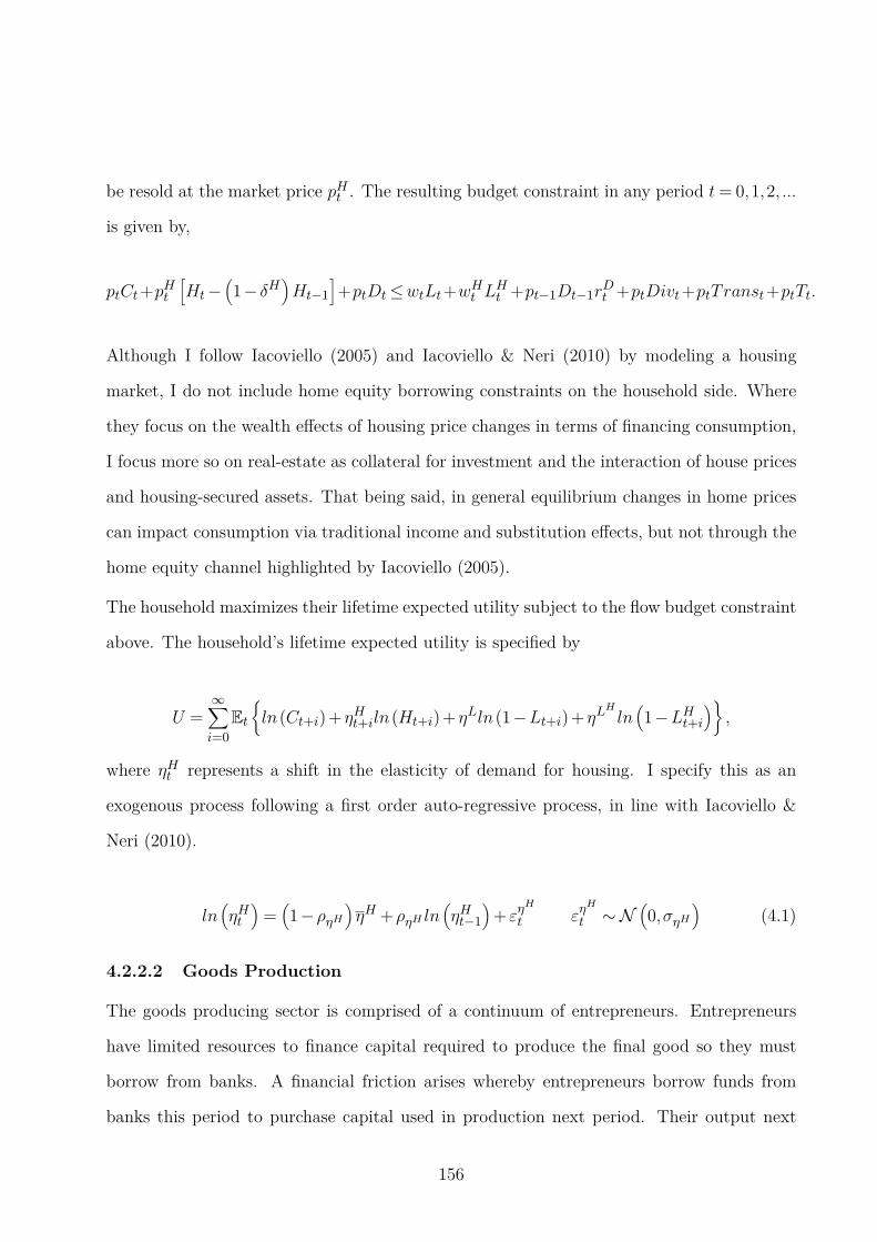
be resold at the market price pHt . The resulting budget constraint in any period t= 0,1,2, ...

is given by,

ptCt+pHt

[

Ht−(

1− δH)

Ht−1

]

+ptDt ≤wtLt+wHt L

Ht +pt−1Dt−1r

Dt +ptDivt+ptTranst+ptTt.

Although I follow Iacoviello (2005) and Iacoviello & Neri (2010) by modeling a housing

market, I do not include home equity borrowing constraints on the household side. Where

they focus on the wealth effects of housing price changes in terms of financing consumption,

I focus more so on real-estate as collateral for investment and the interaction of house prices

and housing-secured assets. That being said, in general equilibrium changes in home prices

can impact consumption via traditional income and substitution effects, but not through the

home equity channel highlighted by Iacoviello (2005).

The household maximizes their lifetime expected utility subject to the flow budget constraint

above. The household’s lifetime expected utility is specified by

U =∞∑

i=0

Et

ln(Ct+i)+ηHt+iln(Ht+i)+ηLln(1−Lt+i)+ηLH

ln(

1−LHt+i)

,

where ηHt represents a shift in the elasticity of demand for housing. I specify this as an

exogenous process following a first order auto-regressive process, in line with Iacoviello &

Neri (2010).

ln(

ηHt)

=(

1−ρηH

)

ηH +ρηH ln(

ηHt−1

)

+ εηH

t εηH

t ∼ N(

0,σηH

)

(4.1)

4.2.2.2 Goods Production

The goods producing sector is comprised of a continuum of entrepreneurs. Entrepreneurs

have limited resources to finance capital required to produce the final good so they must

borrow from banks. A financial friction arises whereby entrepreneurs borrow funds from

banks this period to purchase capital used in production next period. Their output next

156

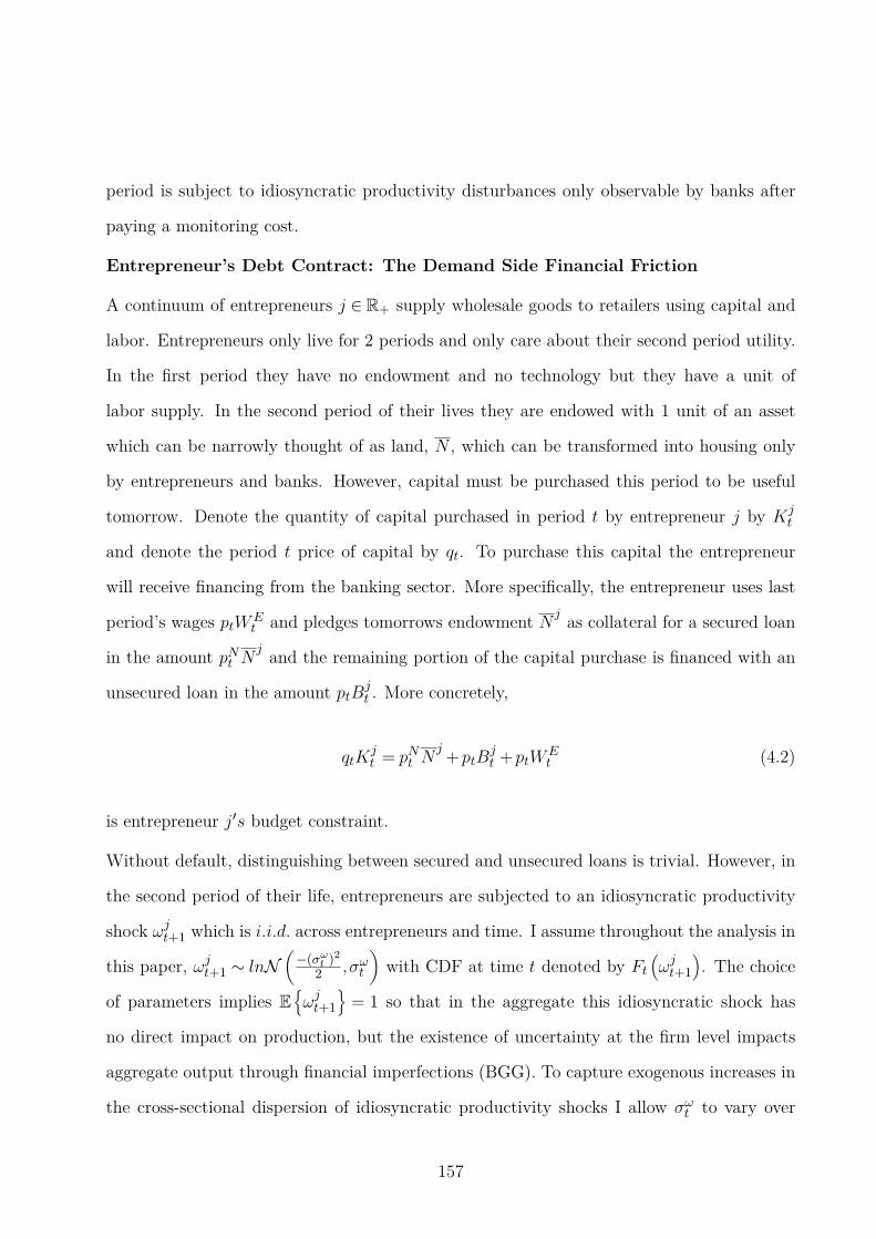
period is subject to idiosyncratic productivity disturbances only observable by banks after

paying a monitoring cost.

Entrepreneur’s Debt Contract: The Demand Side Financial Friction

A continuum of entrepreneurs j ∈ R+ supply wholesale goods to retailers using capital and

labor. Entrepreneurs only live for 2 periods and only care about their second period utility.

In the first period they have no endowment and no technology but they have a unit of

labor supply. In the second period of their lives they are endowed with 1 unit of an asset

which can be narrowly thought of as land, N , which can be transformed into housing only

by entrepreneurs and banks. However, capital must be purchased this period to be useful

tomorrow. Denote the quantity of capital purchased in period t by entrepreneur j by Kjt

and denote the period t price of capital by qt. To purchase this capital the entrepreneur

will receive financing from the banking sector. More specifically, the entrepreneur uses last

period’s wages ptWEt and pledges tomorrows endowment N

jas collateral for a secured loan

in the amount pNt Nj

and the remaining portion of the capital purchase is financed with an

unsecured loan in the amount ptBjt . More concretely,

qtKjt = pNt N

j+ptB

jt +ptW

Et (4.2)

is entrepreneur j′s budget constraint.

Without default, distinguishing between secured and unsecured loans is trivial. However, in

the second period of their life, entrepreneurs are subjected to an idiosyncratic productivity

shock ωjt+1 which is i.i.d. across entrepreneurs and time. I assume throughout the analysis in

this paper, ωjt+1 ∼ lnN(

−(σωt )2

2 ,σωt

)

with CDF at time t denoted by Ft(

ωjt+1

)

. The choice

of parameters implies E

ωjt+1

= 1 so that in the aggregate this idiosyncratic shock has

no direct impact on production, but the existence of uncertainty at the firm level impacts

aggregate output through financial imperfections (BGG). To capture exogenous increases in

the cross-sectional dispersion of idiosyncratic productivity shocks I allow σωt to vary over

157

time. I posit the simple auto-regressive process,

ln(σωt ) = (1−ρσω)σω +ρσω ln(

σωt−1

)

+ εσω

t εσω

t ∼ N (0,σσω) (4.3)

for this demand-side risk shock. Christiano et al. (2013) show that such shocks have played

a significant role in shaping the U.S. business cycle. Moreover, these shocks prove useful in

the empirical analysis of the paper as they provide a structural interpretation for exogenous

increase in the external finance premium.

Since projects are financed before the idiosyncratic productivity shock can be observed by

either the entrepreneur or the bank, entrepreneurs who receive a low productivity value will

default upon their loan. Denote the real gross interest rate on unsecured loans by RL,jt and

denote the gross real return on capital common to all entrepreneurs by RKt+1. Then for any

entrepreneur j, we can define the cut-off value of ωjt+1 by the equation

ωjt+1RKt+1K

jt qt = ptB

jtR

L,jt . (4.4)

This equation defines the minimum level of productivity needed to pay back the unsecured

loan. For entrepreneur j, the loan will be repaid if ωjt+1 ≥ ωjt+1 and will otherwise be

defaulted upon. However, the bank can not observe the level of productivity without paying

an auditing cost in proportion µ ∈ (0,1) to the entrepreneur’s revenue.3 Banks who do not

pay for auditing never find out if the entrepreneur actually received a low productivity draw

or if they simply chose to renege on their loan. Given this arrangement, the optimal debt-

contract dictates that banks will audit only defaulting entrepreneurs and only entrepreneurs

who receive a bad-draw will default on their loans.

To make matters more explicit I define the expected revenue to the bank for loaning ptBjt

to entrepreneur j in (5.17). This expected revenue is comprised of 2 terms, the first of

3This follows from Townsend (1979), but has been popularized in this context by Carlstrom & Fuerst(1997) and BGG.

158

which is non-defaulting loan revenue and the second is revenue net of auditing costs on

non-performing loans.

(

1−Ft(ωjt+1)

)

ptBjtR

Lt

︸ ︷︷ ︸

Non-Defaulting Payoff

+(1−µ)

ˆ ωjt+1

0ωjt+1dFt(ω

jt+1)RKt+1K

jt qt

︸ ︷︷ ︸

Defaulting Payoff

(4.5)

For the bank to be willing to make this loan, this expected pay-off must be at least equal to

bank’s cost of making the loan. In BGG the cost of making the loan is simply the cost of

obtaining the funds via deposits - ptBjtR

Dt . However since the banking sector in this model

has market power this is no longer the case. For the time being simply define the real cost

per dollar loaned by REt .4 Then the incentive compatibility constraint can be expressed as,

ptBjtR

Et =

(

1−Ft(ωjt+1)

)

ptBjtR

Lt +(1−µ)

ˆ ωjt+1

0ωjt+1dFt(ω

jt+1)RKt+1K

jt qt. (4.6)

We can simplify this expression (and the resulting entrepreneur’s optimization problem) by

defining the following terms. First let Gt(ωjt+1) be defined as the expected productivity value

for defaulting entrepreneurs.

Gt(ωjt+1) =

ˆ ωjt+1

0ωjt+1dFt(ω

jt+1) (4.7)

Also let Γt(ωjt+1) be defined as the expected share of entrepreneurial profits going to the

bank gross of auditing costs.

Γt(ωjt+1) =

(

1−Ft(ωjt+1)

)

ωjt+1 +Gt(ωjt+1) (4.8)

Now I can combine (4.6) with (5.16), (5.19) and (5.20) to rewrite the bank’s incentive

4REt is explicitly defined in the description of the banking sector in the appendix using the approach laid

out in Hafstead & Smith (2012)

159

compatibility as,

ptBjtR

Et =

(

Γt(ωjt+1)−µGt(ω

jt+1)

)

RKt+1Kjt qt. (4.9)

We can now formally state the problem faced by entrepreneur j. To keep the debt-contract

tractable, I assume the entrepreneur is risk-neutral with regards to aggregate consumption.

In particular, I assume they seek to maximize their income and then allocate that income

between consumption and housing services. Entrepreneur j therefore seeks to maximize total

income5 subject to the bank’s IC constraint.

maxKj

t ,ωjt+1

(

1−Γt(ωjt+1)

)

RKt+1Kjt qt

subject to[

qtKjt −pNt N

j −ptWEt

]

REt =(

Γt(ωjt+1)−µGt(ω

jt+1)

)

RKt+1Kjt qt

The solution to this optimization problem pins down the cut-off value ωjt+1 and the en-

trepreneur’s demand for capital Kjt .

6 The problem is identical in nature to the problem

entrepreneurs face in BGG who show the optimal debt contract has the property that the

default rate and external finance premium move inversely with net-worth. In this model, the

net-worth component is replaced with the collateral value, implying that ∂ωjt+1/∂pNt < 0 -

finance premiums and default rates will move in the opposite direction of collateral prices.

Aggregate Goods Production

The previous section describes the firm-level behavior in the goods producing sector, specif-

ically it describes the debt-contract problem faced by each producer. In this section, I

describes the industry wide behavior. Each entrepreneur (in the second period of their life)

has access to the production technology, Y jt = ωjtZGt

(

Kjt−1

)αG(

LG,jt

)1−αG, which can be ag-

gregated over due to constant returns to scale. The aggregate goods production technology

5Notice the entrepreneur’s income can be re-written as´∞

ωjt+1

ωjt+1dF (ωj

t+1)RKt+1K

jt qt −

(

1−Ft(ωjt+1)

)

RLt B

jt =

(

1−Γt(ωjt+1)

)

RKt+1K

jt qt where I use (5.16) and (5.20).

6The first order conditions for this problem are in the appendix.

160

in any given period t is specified as

Yt = ZGt(

Kt−1

)αG(

LGt)1−αG

(4.10)

where ZGt is an exogenous technology process which affects all entrepreneurs equally. I

assume this technology follows a first-order autoregressive process.

ln(

ZGt)

= (1−ρZG)ZG+ρZGln(

ZGt−1

)

+ εZG

t εZG

t ∼ N (0,σZG) (4.11)

The gross aggregate real return on holding a unit of capital from period t− 1 to period t is

defined by

RKt =αG

YtKt−1

+(1− δK)Qt

Qt−1, (4.12)

where I utilize the aggregate marginal product of capital from the Cobb-Douglas specification

above - MPK = αGYt

Kt−1.

The labor aggregate in the production function is a composite of labor supplied by the

household, Lt ,and labor supplied by this periods young entrepreneurs, LEt ,

LGt =(

LEt)αE

(

Lt)1−αE

. (4.13)

This implies the wage paid to the household’s labor and the wage paid to entrepreneurial

labor are given by,

Wt = (1−αG)(1−αE)YtLt

(4.14)

WEt = (1−αG)αE

Yt

LEt(4.15)

I calibrate αE = .01 so that in equilibrium the household receives the majority of wages and

variations in collateral values are the primary sources of movement in entrepreneur’s balance

sheets. The aggregate income of entrepreneurs in period t is (1−Γt−1(ωt))RKt Kt−1qt−1.

161

I assume entrepreneurs, like the household, receive utility from consuming both the con-

sumption good and housing services. Unlike households, entrepreneurs have the ability to

transform their endowment of ‘land’ - Nj

- into non-tradable housing. Recall however, this

endowment was leveraged last period to secure a loan in the amount pNt−1Nj. Hence, en-

trepreneurs who are able, choose to payback the secured loan with interest pNt−1NjrDt−1 and

then convert Nj

into housing services one for one. If they don’t payback the secured loan

then they default on this contract and the bank takes possession of the collateral Nj.

I assume in the aggregate, all the entrepreneurs who did not default on their unsecured

loan, payback their secured loan and use the rest of their income on the consumption good.

Those who defaulted on the unsecured loan have lost all income and hence do not consume

anything. More specifically, the aggregate real consumption of entrepreneurs is given by

CEt = (1−Γt−1(ωt))RKt Kt−1Qt−1 − (1−Ft−1(ωt))P

Nt−1N

jRDt−1. (4.16)

“What micro-level preferences would give rise to this aggregate consumption behavior?” is

an interesting question. In the appendix I describe one possible micro-structure that would

lead to this aggregate consumption behavior . An appealing aspect of this description is the

existence of a single default rate in the economy.7

4.2.2.3 New Housing Production

I assume new housing is produced in a purely competitive market and free from financial fric-

tions. In particular, housing producers combine labor LHt with housing specific technology,

ZHt in the production technology,

HNewt = ZHt

(

LHt)1−αH

(4.17)

7That is to say, the default rate on unsecured loans is the same as the default rate on secured loans. Ichoose this as a starting point although this assumption can be relaxed.

162

where

ln(

ZHt)

= (1−ρZH )ZH +ρZH ln(

ZHt−1

)

+ εZH

t εZH

t ∼ N (0,σZH ) . (4.18)

I model housing specific technology independent of technology in the goods producing sector

since much of the economic growth over the last two decades has been IT-driven and housing

production is a non IT-intensive industry. Moreover, this specification allows for goods

technology process, ZGt , to play a significant role in determining output without implying a

counterfactual negative correlation between home prices and GDP (see for example Davis &

Heathcote (2005)). The resulting demand for labor from the housing sector takes the form

WHt = (1−αH)PHt

HNewt

LHt. (4.19)

4.2.2.4 Banking Sector: The Supply Side Financial Friction

There are a unit measure of banks in the model each belonging to one of two types. I dis-

tinguish bank types by a superscript “P” for productive banks and a superscript “U” for

unproductive banks (who make up ν share of the population). Productive banks represent

the Large commercial banks in the data. These banks are more productive with repossessed

collateral pledged by entrepreneurs to secure loans and hence value these housing-secured

assets more than their unproductive counterparts. However, this efficiency creates a moral

hazard problem for borrowers due to the possibility of productive banks wrongfully repos-

sessing collateral and absconding with the profits. If this occurs, the entrepreneur’s only

recourse is to take the productive banks accumulated capital. To this extent, bank-capital

mitigates the moral hazard concerns and allows the productive banks to hold more of these

collateralized assets. An amplification effect emerges from the endogenous tightening and

loosening of this moral hazard constraint which forces productive banks to adjust their hold-

ing of collateralized assets in response to movements in home prices.

163

For ease of exposition I describe factors common to both types of bank before describing each

type’s optimizing behavior. In particular, all banks have some degree of market power, face

a balance sheet constraint and remit a fraction of profits each period back to the household

in the form of dividends and various transfers. In what follows I generically refer to bank i

to reference one of the infinitely many identical banks within either type.

Each bank possesses a degree of market power which is captured by assuming a Dixit-Stiglitz

type aggregator function. As Hafstead & Smith (2012) point out, this has the simplifying

feature that all banks serve all entrepreneurs and therefore face the same ex-ante and ex-post

default rates. More specifically, aggregate loans are a CES index

Bt =

(ˆ 1

0Bt(i)

θB−1θB

) θBθB−1

(4.20)

where θB is the elasticity of substitution between different bank loans and is calibrated to

match aggregate lending rates. The corresponding price index which is dual8 to this quantity

index is given by

rBt =

(ˆ 1

0rBt (i)1−θB

) 11−θB

. (4.21)

This specification of the aggregate indexes implies each bank i of type T ∈ P,U faces the

downward sloping demand for loans,

BTt (i) =

rB,Tt (i)

rBt

−θB

Bt. (4.22)

Each bank i must not only satisfy their demand for loans, but they must also abide to the

balance sheet constraint,

ptBTt (i)+pNt N

Tt (i) = ptD

Tt (i)+pt−1BK

Tt−1(i) (4.23)

8Duality here refers to the price and quantity indexes which satisfy Fisher’s factor reversal test,´ 1

0 rBt (i)Bt(i)di= rB

t Bt.

164

which simply states that assets (bank loans) must equal liabilities (bank deposits) plus bank

capital, respectively.

Since banks use share holder’s retained earnings to fund risky loans, I assume shareholders

(households) require compensation. More specifically, each period the bank is allowed (by

the central bank) to expose a fraction ψt of bank capital to cover expected losses on unsecured

defaulted loans. Each period t, the fraction of loans that actually default is given by Ft−1(ωt).

Hence, each period the bank transfers the nominal payment

ptTransTt (i) = Ft−1(ωt)pt−1ψt−1BK

Tt−1(i) (4.24)

to shareholders in order to compensate them for the capital that was exposed to covering

losses on loans originated in period t− 1. In this sense, the transfer to shareholders occurs

only on realized, or ex-post, loan losses. Combining this transfer payment with dividend

payments, bank capital evolves according to the following law of motion.

ptBKTt (i) = γTt ptΠ

Tt (i)−ptTrans

Tt (i)+(1− δBK)pt−1BK

Tt−1(i) (4.25)

To summarize this, banks of type T pay out a time varying fraction γTt of period t profits as

dividends and invest the remaining fraction in bank capital. Additionally, banks compensate

shareholders for exposing retained earnings to potential losses via ptTransTt and lose a

fraction of bank capital to depreciation. Following Gerali et al. (2010), I assume bank

investment decisions are made independently from bank profit maximization, however, I

assume this fraction is time varying. In particular, I assume that γTt = γT

ptΠTt

so that each

period a constant amount of new equity is injected into the banks from shareholders. This

implies realistically that banks respond to falling profits by paying out a smaller share of

profits in dividends. Before proceeding to a specific description of each type of bank’s

problem, it useful to summarize these transfers by defining net investment in the banking

165

sector.

IBKt =∑

T∈P,U

sT(

γTt ptΠTt −ptTrans

Tt

)

where sT =

ν if T = U

1−ν if T = P

(4.26)

Productive Bank

The productive bank enters each period t with inflows consisting of maturing unsecured

loans rB,Pt−1 (i)ptBPt−1(i) and maturing secured loans pNt−1N

Pt−1r

Dt−1, of which, (1−Ft−1(ωt))

will be repaid in full. Denote the real income of all borrowers who are unable to repay

last periods loan by Φt−1(ωt). The productive bank will receives the fractionBP

t−1(i)Bt−1

of

φt−1(ωt) net of auditing costs µ for the unsecured loan defaults. Additionally, the productive

bank repossesses Ft−1(ωt)NPt−1(i), which is the collateral posted on the secured loans who

defaulted. This repossessed collateral is transformed in to housing using the technology

common to all banks, HRt (i) = ZRNP

t−1(i). Finally, the productive bank also has incoming

deposits totaling ptDPt (i). At the same time, the productive bank has outflows of newly

originated unsecured and secured loans totaling ptBPt (i) +pNt N

Pt (i) and maturing deposits

from period t− 1 totaling pt−1DPt−1(i)rDt−1. This is stated more concisely below in (4.30)

which defines the productive bank’s period t nominal profits.

ptΠPt (i) = (1−Ft−1(ωt))r

B,Pt−1 (i)ptB

Pt−1(i)+(1−µ)

BPt−1(i)

Bt−1ptΦt−1(ωt)

+(1−Ft−1(ωt))pNt−1N

Pt−1(i)rDt−1 +Ft−1(ωt)p

Ht Z

RNPt−1(i) (4.27)

−ptBPt (i)−pNt N

Pt (i)−pt−1D

Pt−1(i)rDt−1 +ptDt(i)

The productive bank’s ability to liquidate repossessed collateral - NPt at zero marginal cost

raises a moral hazard. In particular, if the productive bank were to claim default on all the

secured loans originated in period t and repossess the collateral the following period, they

would earn a gross real return totaling NPt Et

ZRPH

t+1−(1−Ft(ωt+1)RDt P

Nt )

PNt

. The first term

166

represents income from the selling the unlawfully repossessed collateral and the second term

subtracts the foregone income that would have been received from entrepreneurs paying back

their loans. I assume a fraction of this return will be lost when taken so that productive

banks only net a fraction ψN,Pt of this return. This varies stochastically according to the

AR(1) process.

ln(

ψN,Pt

)

=(

1−ρψN,P

)

ψN,P +ρψN,P ln(

ψN,Pt−1

)

+ εψN,P

t εψN,P

t ∼ N(

0,σψN,P

)

(4.28)

These disturbances provide a model equivalent to the large bank share shock from that will

be analyzed in the VAR.

If the productive bank chooses to abscond with the assets, entrepreneurs are entitled to

the remaining equity of the bank after preferred shareholders (households) receive their risk

premium. Hence, entrepreneurs would be entitled to a claim of (1−ψtFt(ωt+1))BKPt (i).

Thus, the incentive for productive banks to claim default and abscond with these housing-

secured assets is eliminated when the equity claims of exploited entrepreneurs exceeds the

gross return on unlawful liquidations.

(1−ψtFt(ωt+1))BKPt (i)

︸ ︷︷ ︸

Equity Claim of Exploited Entrepreneurs

≥NPt Et

ZRPHt+1 − (1−Ft(ωt+1)RDt PNt )

PNt

ψN,Pt

︸ ︷︷ ︸

Gross Return on Unlawful Repossessions

(4.29)

When (4.29) holds with equality, the productive bank will be limited in how many housing-

secured assets it can hold. Moreover, this constraint will endogenously loosen and tighten

in response to various macroeconomic shocks which affect home prices or default rates. Let

Λt denote the household’s stochastic discount factor used for valuing future real payments.

The problem faced by the productive bank is then defined below.

max

rB,Pt+j (i),BP

t+j(i),NPt+j(i),DP

t+j(i)∞

j=0

∞∑

j=0

Et

Λt+jΠPt+j(i)

subject to (4.22), (4.23), (4.29)

167

Due to the complications that arise from solving a model with an occasionally binding

constraint, I calibrate the model so that the productive bank’s moral hazard constraint

binds in the non-stochastic steady-state.

Unproductive Bank

The unproductive bank is identical to the productive bank with one noticeable exception -

they are less productive. To make matters more concrete, when a secured loan defaults the

unproductive bank repossesses collateral Ft−1(ωt)NUt−1(i). Unlike their productive counter-

parts, the unproductive bank liquidates this collateral while bearing an increasing marginal

cost. On defaulted secured loans, the unproductive bank transforms repossessed collateral

into housing yielding revenue pHt ZRNU

t−1(i) at a resource cost of ptµR,U

(

NUt−1(i)

)χR,U

. This

captures the heterogeneity between commercial banks (empirically found by (Wheelock &

Wilson, 2012; Bos & Kolari, 2013)) with regards to their ability to evaluate and trade off-

balance sheet assets. Most notably, as unproductive banks increase their holding of these

assets, the value of the assets will fall due to the increasing marginal cost. Hence, the market

liquidity of such assets depends on the distribution of these assets (i.e. it depends on who

is holding the assets). A point first made by KM and applied to here to housing backed

securities within this model.

With this exception, the unproductive bank’s profit function is very similar to the productive

bank’s stated below.

ptΠUt (i) = (1−Ft−1(ωt))r

B,Ut−1 (i)ptB

Ut−1(i)+(1−µ)

BUt−1(i)

Bt−1ptΦt−1(ωt)

+(1−Ft−1(ωt))pNt−1N

Ut−1(i)rD,Ut−1 (4.30)

+Ft−1(ωt)

[

pHt ZRNU

t−1(i)−ptµR,U

(

NUt−1(i)

)χR,U]

−ptBUt (i)−χB,UBU

t (i)−pNt NUt (i)−pt−1D

Ut−1(i)rDt−1 +ptD

Ut (i)

Notice the lack of productivity spills over to unsecured loans. The parameter χB,U is cal-

168

ibrated to match the average share of resources allocated to financial intermediation. The

increasing resource cost of repossessing collateral implies the unproductive bank is not sub-

ject to a moral hazard constraint. In particular, if any single unproductive bank i attempted

to purchase a large amount of these assets at a given market price pNt and falsely claim

default, their cost of liquidating the assets would exceed what they paid for them. Therefore

the existence of these increasing marginal cost eliminates any incentive to steal away these

assets.

Let Λt denote the household’s stochastic discount factor used for valuing future real pay-

ments. The problem faced by the unproductive bank is then defined below.

max

rB,Ut+j (i),BU

t+j(i),NUt+j(i),DU

t+j(i)∞

j=0

∞∑

j=0

Et

Λt+jΠUt+j(i)

subject to (4.22), (4.23)

4.2.2.5 Central Bank

The central bank is charged with setting a macroprudential policy rule and a monetary

policy rule. The macroprudential policy instrument is the regulatory maximum share of

capital that can be allocated to loan losses. This essentially controls the amount of owners

equity the bank can allocate to cover loan losses. Here, I assume the central bank simply

sets this to a constant level,

ψt = ψ. (4.31)

As for the monetary policy instrument I assume the central bank follows the simple interest

rate rule whereby the rate on one-period deposits adjusts to itself lagged, the inflation rate,

and the growth rate of real GDP:

(

rDt

rD

)

=

(

rDt−1

rD

)ρr(

πtπ

)ψπ(

GDPt¯GDPt−1

)ψGDP

. (4.32)

169

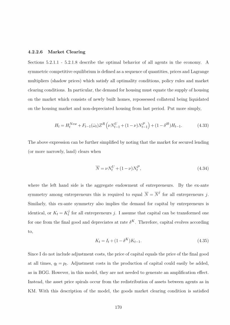
4.2.2.6 Market Clearing

Sections 5.2.1.1 - 5.2.1.8 describe the optimal behavior of all agents in the economy. A

symmetric competitive equilibrium is defined as a sequence of quantities, prices and Lagrange

multipliers (shadow prices) which satisfy all optimality conditions, policy rules and market

clearing conditions. In particular, the demand for housing must equate the supply of housing

on the market which consists of newly built homes, repossessed collateral being liquidated

on the housing market and non-depreciated housing from last period. Put more simply,

Ht =HNewt +Ft−1(ωt)Z

R(

νNUt−1 +(1−ν)NP

t−1

)

+(1− δH)Ht−1. (4.33)

The above expression can be further simplified by noting that the market for secured lending

(or more narrowly, land) clears when

N = νNUt +(1−ν)NP

t , (4.34)

where the left hand side is the aggregate endowment of entrepreneurs. By the ex-ante

symmetry among entrepreneurs this is required to equal N = Nj

for all entrepreneurs j.

Similarly, this ex-ante symmetry also implies the demand for capital by entrepreneurs is

identical, or Kt =Kjt for all entrepreneurs j. I assume that capital can be transformed one

for one from the final good and depreciates at rate δK . Therefore, capital evolves according

to,

Kt = It+(1− δK)Kt−1. (4.35)

Since I do not include adjustment costs, the price of capital equals the price of the final good

at all times, qt = pt. Adjustment costs in the production of capital could easily be added,

as in BGG. However, in this model, they are not needed to generate an amplification effect.

Instead, the asset price spirals occur from the redistribution of assets between agents as in

KM. With this description of the model, the goods market clearing condition is satisfied

170

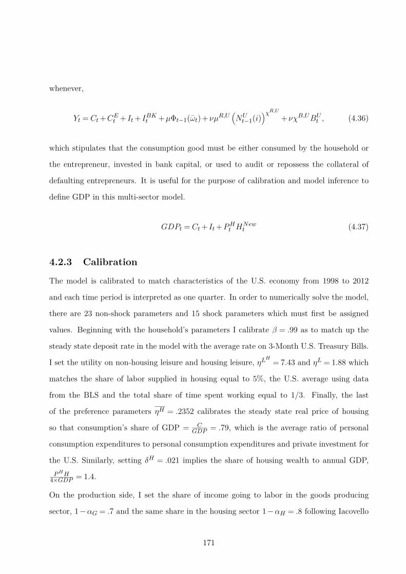
whenever,

Yt = Ct+CEt + It+ IBKt +µΦt−1(ωt)+νµR,U(

NUt−1(i)

)χR,U

+νχB,UBUt , (4.36)

which stipulates that the consumption good must be either consumed by the household or

the entrepreneur, invested in bank capital, or used to audit or repossess the collateral of

defaulting entrepreneurs. It is useful for the purpose of calibration and model inference to

define GDP in this multi-sector model.

GDPt = Ct+ It+PHt HNewt (4.37)

4.2.3 Calibration

The model is calibrated to match characteristics of the U.S. economy from 1998 to 2012

and each time period is interpreted as one quarter. In order to numerically solve the model,

there are 23 non-shock parameters and 15 shock parameters which must first be assigned

values. Beginning with the household’s parameters I calibrate β = .99 as to match up the

steady state deposit rate in the model with the average rate on 3-Month U.S. Treasury Bills.

I set the utility on non-housing leisure and housing leisure, ηLH

= 7.43 and ηL = 1.88 which

matches the share of labor supplied in housing equal to 5%, the U.S. average using data

from the BLS and the total share of time spent working equal to 1/3. Finally, the last

of the preference parameters ηH = .2352 calibrates the steady state real price of housing

so that consumption’s share of GDP = CGDP = .79, which is the average ratio of personal

consumption expenditures to personal consumption expenditures and private investment for

the U.S. Similarly, setting δH = .021 implies the share of housing wealth to annual GDP,

PHH4×GDP = 1.4.

On the production side, I set the share of income going to labor in the goods producing

sector, 1−αG = .7 and the same share in the housing sector 1−αH = .8 following Iacovello

171

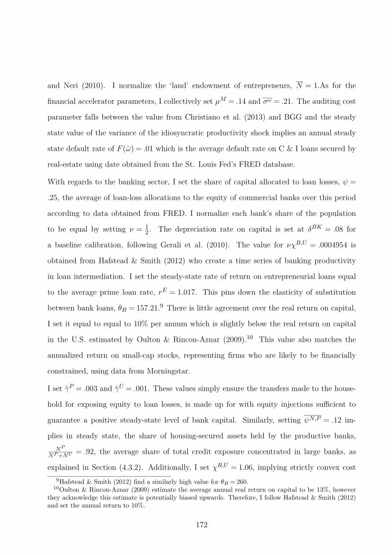
and Neri (2010). I normalize the ‘land’ endowment of entrepreneurs, N = 1.As for the

financial accelerator parameters, I collectively set µM = .14 and σω = .21. The auditing cost

parameter falls between the value from Christiano et al. (2013) and BGG and the steady

state value of the variance of the idiosyncratic productivity shock implies an annual steady

state default rate of F (ω) = .01 which is the average default rate on C & I loans secured by

real-estate using date obtained from the St. Louis Fed’s FRED database.

With regards to the banking sector, I set the share of capital allocated to loan losses, ψ =

.25, the average of loan-loss allocations to the equity of commercial banks over this period

according to data obtained from FRED. I normalize each bank’s share of the population

to be equal by setting ν = 12 . The depreciation rate on capital is set at δBK = .08 for

a baseline calibration, following Gerali et al. (2010). The value for νχB,U = .0004954 is

obtained from Hafstead & Smith (2012) who create a time series of banking productivity

in loan intermediation. I set the steady-state rate of return on entrepreneurial loans equal

to the average prime loan rate, rE = 1.017. This pins down the elasticity of substitution

between bank loans, θB = 157.21.9 There is little agreement over the real return on capital,

I set it equal to equal to 10% per annum which is slightly below the real return on capital

in the U.S. estimated by Oulton & Rincon-Aznar (2009).10 This value also matches the

annualized return on small-cap stocks, representing firms who are likely to be financially

constrained, using data from Morningstar.

I set γP = .003 and γU = .001. These values simply ensure the transfers made to the house-

hold for exposing equity to loan losses, is made up for with equity injections sufficient to

guarantee a positive steady-state level of bank capital. Similarly, setting ψN,P = .12 im-

plies in steady state, the share of housing-secured assets held by the productive banks,

NP

NP +NU = .92, the average share of total credit exposure concentrated in large banks, as

explained in Section (4.3.2). Additionally, I set χR,U = 1.06, implying strictly convex cost

9Hafstead & Smith (2012) find a similarly high value for θB = 260.10Oulton & Rincon-Aznar (2009) estimate the average annual real return on capital to be 13%, however

they acknowledge this estimate is potentially biased upwards. Therefore, I follow Hafstead & Smith (2012)and set the annual return to 10%.

172

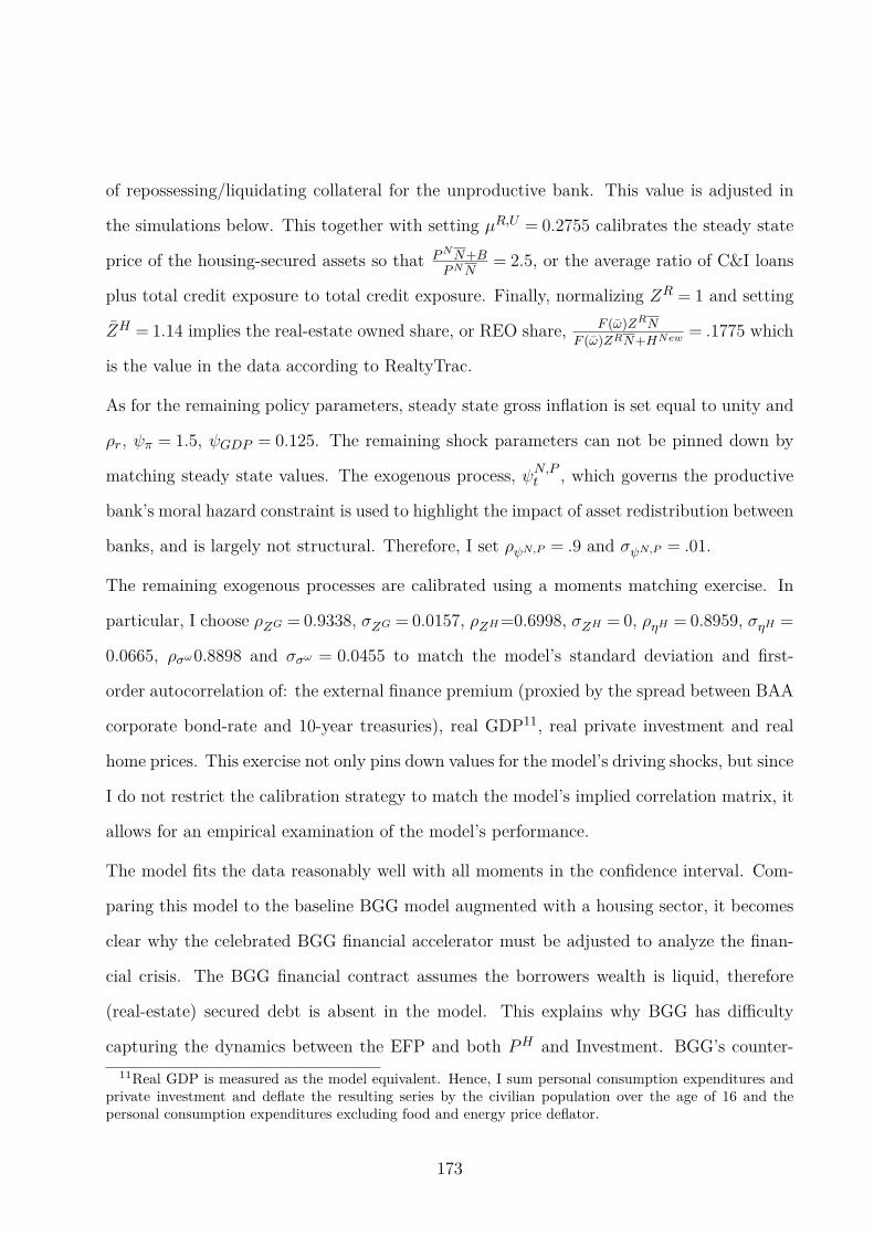
of repossessing/liquidating collateral for the unproductive bank. This value is adjusted in

the simulations below. This together with setting µR,U = 0.2755 calibrates the steady state

price of the housing-secured assets so that PNN+BPNN

= 2.5, or the average ratio of C&I loans

plus total credit exposure to total credit exposure. Finally, normalizing ZR = 1 and setting

ZH = 1.14 implies the real-estate owned share, or REO share, F (ω)ZRN

F (ω)ZRN+HNew = .1775 which

is the value in the data according to RealtyTrac.

As for the remaining policy parameters, steady state gross inflation is set equal to unity and

ρr, ψπ = 1.5, ψGDP = 0.125. The remaining shock parameters can not be pinned down by

matching steady state values. The exogenous process, ψN,Pt , which governs the productive

bank’s moral hazard constraint is used to highlight the impact of asset redistribution between

banks, and is largely not structural. Therefore, I set ρψN,P = .9 and σψN,P = .01.

The remaining exogenous processes are calibrated using a moments matching exercise. In

particular, I choose ρZG = 0.9338, σZG = 0.0157, ρZH =0.6998, σZH = 0, ρηH = 0.8959, σηH =

0.0665, ρσω0.8898 and σσω = 0.0455 to match the model’s standard deviation and first-

order autocorrelation of: the external finance premium (proxied by the spread between BAA

corporate bond-rate and 10-year treasuries), real GDP11, real private investment and real

home prices. This exercise not only pins down values for the model’s driving shocks, but since

I do not restrict the calibration strategy to match the model’s implied correlation matrix, it

allows for an empirical examination of the model’s performance.

The model fits the data reasonably well with all moments in the confidence interval. Com-

paring this model to the baseline BGG model augmented with a housing sector, it becomes

clear why the celebrated BGG financial accelerator must be adjusted to analyze the finan-

cial crisis. The BGG financial contract assumes the borrowers wealth is liquid, therefore

(real-estate) secured debt is absent in the model. This explains why BGG has difficulty

capturing the dynamics between the EFP and both PH and Investment. BGG’s counter-

11Real GDP is measured as the model equivalent. Hence, I sum personal consumption expenditures andprivate investment and deflate the resulting series by the civilian population over the age of 16 and thepersonal consumption expenditures excluding food and energy price deflator.

173

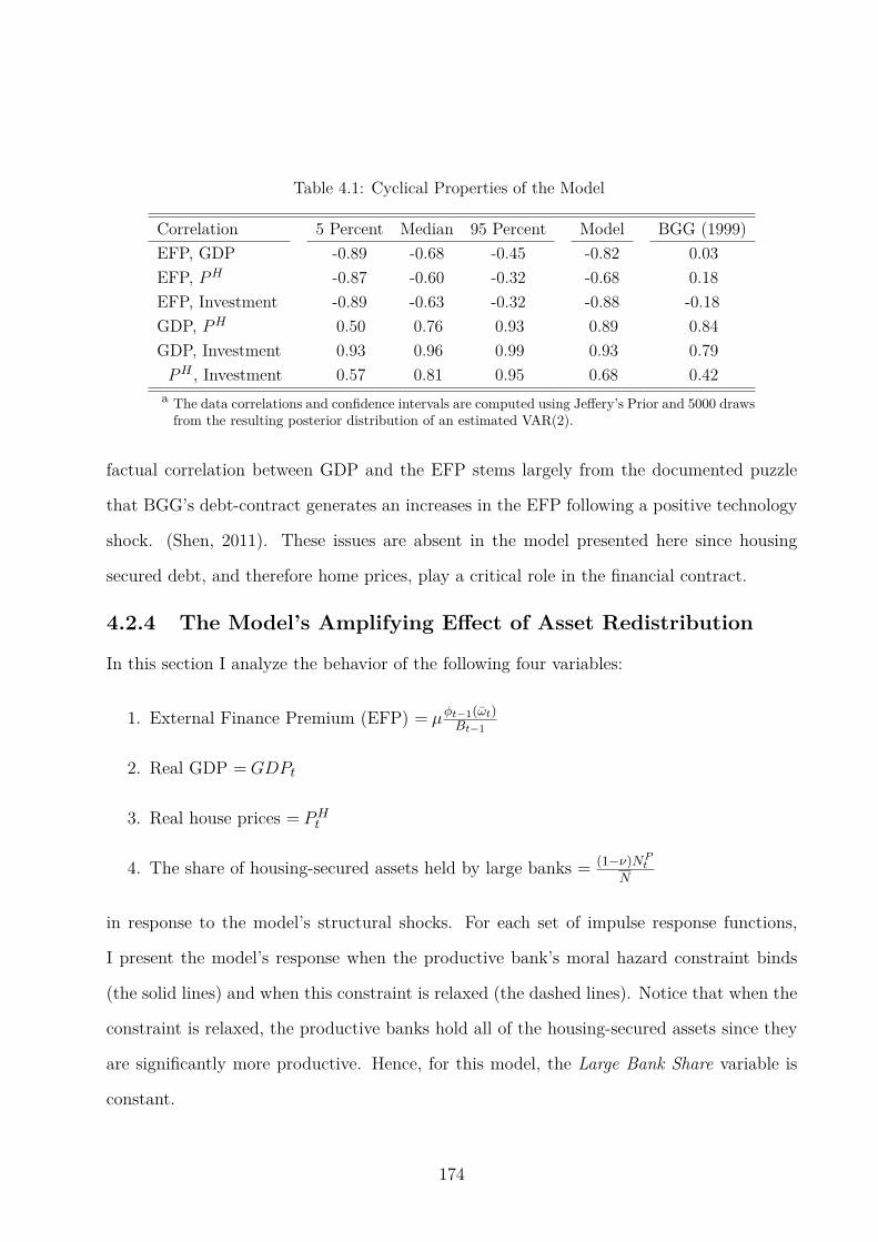
Table 4.1: Cyclical Properties of the Model

Correlation 5 Percent Median 95 Percent Model BGG (1999)

EFP, GDP -0.89 -0.68 -0.45 -0.82 0.03

EFP, PH -0.87 -0.60 -0.32 -0.68 0.18

EFP, Investment -0.89 -0.63 -0.32 -0.88 -0.18

GDP, PH 0.50 0.76 0.93 0.89 0.84

GDP, Investment 0.93 0.96 0.99 0.93 0.79

PH , Investment 0.57 0.81 0.95 0.68 0.42

a The data correlations and confidence intervals are computed using Jeffery’s Prior and 5000 drawsfrom the resulting posterior distribution of an estimated VAR(2).

factual correlation between GDP and the EFP stems largely from the documented puzzle

that BGG’s debt-contract generates an increases in the EFP following a positive technology

shock. (Shen, 2011). These issues are absent in the model presented here since housing

secured debt, and therefore home prices, play a critical role in the financial contract.

4.2.4 The Model’s Amplifying Effect of Asset Redistribution

In this section I analyze the behavior of the following four variables:

1. External Finance Premium (EFP) = µφt−1(ωt)Bt−1

2. Real GDP =GDPt

3. Real house prices = PHt

4. The share of housing-secured assets held by large banks = (1−ν)NPt

N

in response to the model’s structural shocks. For each set of impulse response functions,

I present the model’s response when the productive bank’s moral hazard constraint binds

(the solid lines) and when this constraint is relaxed (the dashed lines). Notice that when the

constraint is relaxed, the productive banks hold all of the housing-secured assets since they

are significantly more productive. Hence, for this model, the Large Bank Share variable is

constant.

174

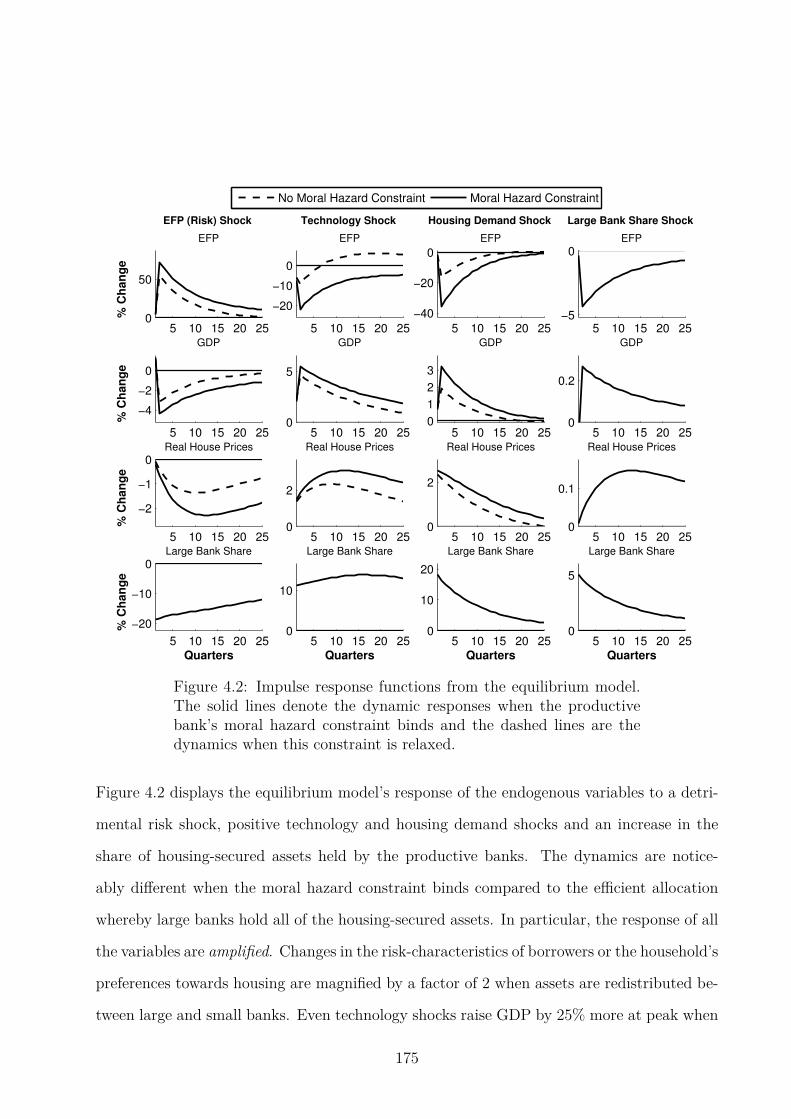
5 10 15 20 250

50

% C

han

ge

EFP (Risk) Shock

EFP

No Moral Hazard Constraint Moral Hazard Constraint

5 10 15 20 25

−20

−10

0

Technology Shock

EFP

5 10 15 20 25

−40

−20

0

Housing Demand Shock

EFP

5 10 15 20 25−5

0

Large Bank Share Shock

EFP

5 10 15 20 25

−4

−2

0

% C

han

ge

GDP

5 10 15 20 250

5

GDP

5 10 15 20 250

1

2

3

GDP

5 10 15 20 250

0.2

GDP

5 10 15 20 25

−2

−1

0

% C

han

ge

Real House Prices

5 10 15 20 250

2

Real House Prices

5 10 15 20 250

2

Real House Prices

5 10 15 20 250

0.1

Real House Prices

5 10 15 20 25

−20

−10

0

% C

han

ge

Quarters

Large Bank Share

5 10 15 20 250

10

Quarters

Large Bank Share

5 10 15 20 250

10

20

Quarters

Large Bank Share

5 10 15 20 250

5

Quarters

Large Bank Share

Figure 4.2: Impulse response functions from the equilibrium model.The solid lines denote the dynamic responses when the productivebank’s moral hazard constraint binds and the dashed lines are thedynamics when this constraint is relaxed.

Figure 4.2 displays the equilibrium model’s response of the endogenous variables to a detri-

mental risk shock, positive technology and housing demand shocks and an increase in the

share of housing-secured assets held by the productive banks. The dynamics are notice-

ably different when the moral hazard constraint binds compared to the efficient allocation

whereby large banks hold all of the housing-secured assets. In particular, the response of all

the variables are amplified. Changes in the risk-characteristics of borrowers or the household’s

preferences towards housing are magnified by a factor of 2 when assets are redistributed be-

tween large and small banks. Even technology shocks raise GDP by 25% more at peak when

175

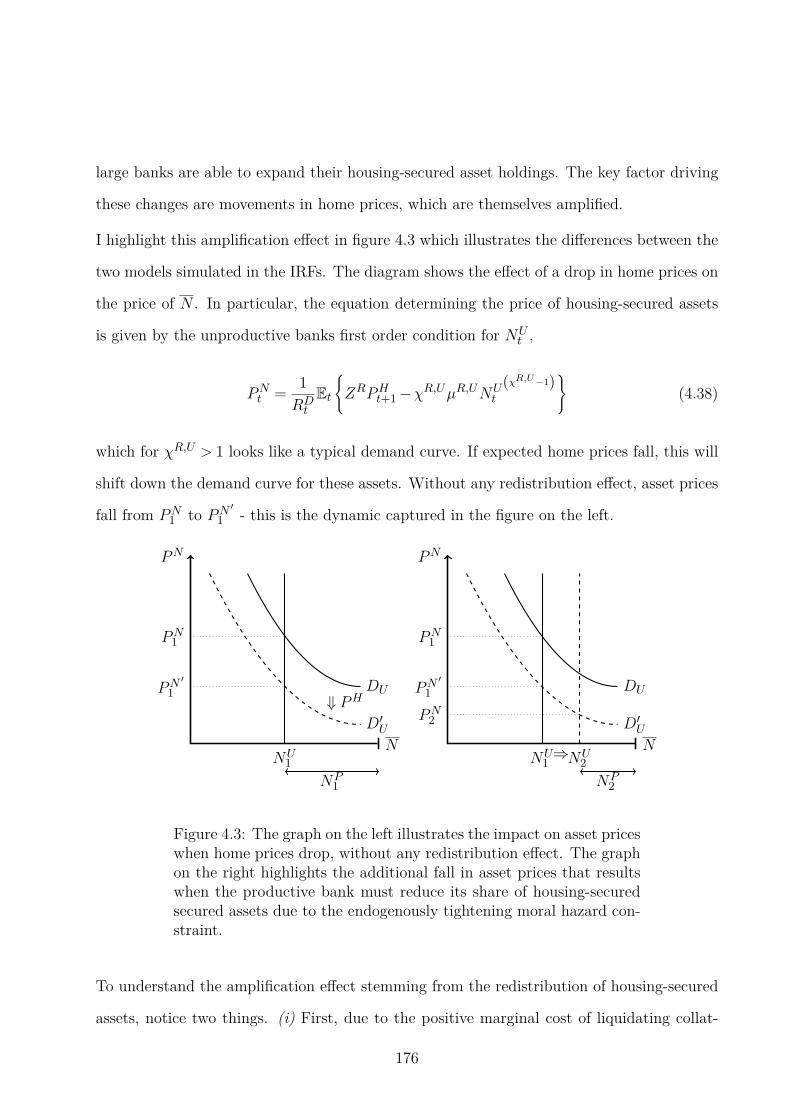
large banks are able to expand their housing-secured asset holdings. The key factor driving

these changes are movements in home prices, which are themselves amplified.

I highlight this amplification effect in figure 4.3 which illustrates the differences between the

two models simulated in the IRFs. The diagram shows the effect of a drop in home prices on

the price of N . In particular, the equation determining the price of housing-secured assets

is given by the unproductive banks first order condition for NUt ,

PNt =1

RDtEt

ZRPHt+1 −χR,UµR,UNU(χR,U−1)

t

(4.38)

which for χR,U > 1 looks like a typical demand curve. If expected home prices fall, this will

shift down the demand curve for these assets. Without any redistribution effect, asset prices

fall from PN1 to PN′

1 - this is the dynamic captured in the figure on the left.

N

PN

NU1

NP1

DU

PN1

D′U

PN′

1 ⇓ PH

N

PN

NU1 NU

2

NP2

DU

PN1

D′U

PN′

1

PN2

⇒

Figure 4.3: The graph on the left illustrates the impact on asset priceswhen home prices drop, without any redistribution effect. The graphon the right highlights the additional fall in asset prices that resultswhen the productive bank must reduce its share of housing-securedsecured assets due to the endogenously tightening moral hazard con-straint.

To understand the amplification effect stemming from the redistribution of housing-secured

assets, notice two things. (i) First, due to the positive marginal cost of liquidating collat-

176

eral, asset prices fall by more (in percentage terms) than expected home prices. That is,

EPNt ,EtPH

t+1 > 1.

EPNt ,EtPH

t+1 =∂PNt

∂Et

PHt+1

Et

PHt+1

PNt=

ZREt

PHt+1

ZREt

PHt+1

−χR,UµR,UNU(χR,U −1)t

> 1 (4.39)

(ii) Second, the debt contract described in section 4.2.2.2 shows that as the value of the

entrepreneur’s pledgeable assets falls, the probability of default increases.12

∂Ft(ωjt+1)

∂PNt=∂Ft(ω

jt+1)

∂ωjt+1

∂ωjt+1

∂PNt< 0 (4.40)

These two effects, (i) and (ii) (Eqs. 4.39 and 4.40 ), both act to tighten the binding moral

hazard constraint for the productive bank (Eq. (4.29)) and hence the large bank share falls.

This is illustrated in the graph on the right of figure 4.3. In particular, a drop in home prices

induces not only a direct fall in asset prices from PN1 to PN′

1 but a further drop to PN2 due

to an endogenous reduction in NPt (and the downward sloping demand for NU

t due to the

strictly convex costs). This is the beginning a multiplier effect of sorts. As PNt falls by more

than Et

PHt+1

, the moral hazard constraint tightens further inducing further reductions in

NPt . All the while, as these forces act to push down the value of secured debt, borrower’s

face an increasing external finance premium. This is the amplification effect highlighted by

the difference between the 2 sets of IRFs in figure 4.2.

This static multiplier effect from asset redistribution may be easiest to spot when I exoge-

nously increase the share of assets held by the productive bank. The dynamics following

this exogenous shock are shown in the the last column of IRFs in figure 4.2. Although, the

shock is set to increase NPt by only 1% the period the shock hits, NP

t increases more than 5

times as much, above 5%. Again, this amplified response is driven by the asset redistribution

illustrated in figure 4.3. When NPt increases there are two immediate effects, as explained

12The first partial derivative is positive due to the monotonicity of CDFs and the second partial derivativeis negative due to the structure of the optimal debt contract.

177

by equations 4.39 and 4.40, both of which act to expound this increase in the productive

bank’s share of housing-secured assets.

One common theme through all the impulse response functions is an amplification effect

stemming from asset redistribution. Although, I have highlighted the static amplification,

there is also a dynamic feature at work which makes the moral-hazard constrained model

more persistent. Since repossessed collateral ultimately is liquidated on the real-estate mar-

ket, this increase in supply lowers home prices into the future to the extent that housing

does not depreciate immediately. These effects re-enforce one another over time. Ultimately

though, these dynamic amplification effects are powered by restarting, period by period, the

engine that drives the static multiplier.

4.3 VAR Tests of the Model’s Amplification Mecha-

nism

In this section, I estimate a series of VAR models to examine the empirical plausibility of the

model’s predictions. The variables included in the VARs are the same variables examined in

the model’s impulse response functions: the external finance premium, real GDP, real home

prices and the share of total credit exposure concentrated in large banks. All variables are

available at a quarterly frequency from 1998:Q2 to 2012:Q4.13 As specified in log-levels, the

Schwarz Bayesian information criterion selects 2 lags for the VAR. In what follows I first

lay-out the model’s testable predictions, then I go on to describe the data and the structural

identification before presenting the impulse response functions for the various models.

4.3.1 The Model’s Empirical Implications

The DSGE model developed in the previous section posits an amplification effect stemming

from the redistribution of assets between large and small banks. In particular, the amplifica-

tion mechanism posits that an initial economic downturn, in which home prices fall, causes

13The time series is limited by the availability of net credit exposure data from the OCC’s QuarterlyDerivatives Report. However, for the removal of trends, I use data going back to 1975:Q1

178

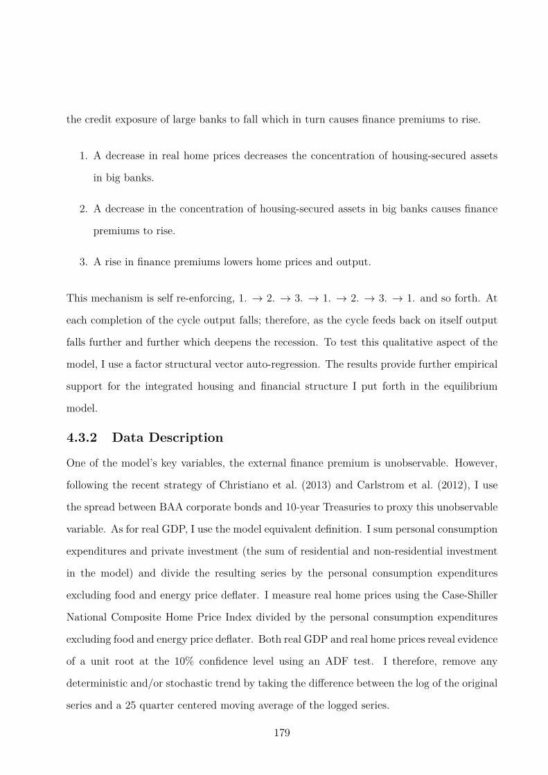
the credit exposure of large banks to fall which in turn causes finance premiums to rise.

1. A decrease in real home prices decreases the concentration of housing-secured assets

in big banks.

2. A decrease in the concentration of housing-secured assets in big banks causes finance

premiums to rise.

3. A rise in finance premiums lowers home prices and output.

This mechanism is self re-enforcing, 1. → 2. → 3. → 1. → 2. → 3. → 1. and so forth. At

each completion of the cycle output falls; therefore, as the cycle feeds back on itself output

falls further and further which deepens the recession. To test this qualitative aspect of the

model, I use a factor structural vector auto-regression. The results provide further empirical

support for the integrated housing and financial structure I put forth in the equilibrium

model.

4.3.2 Data Description

One of the model’s key variables, the external finance premium is unobservable. However,

following the recent strategy of Christiano et al. (2013) and Carlstrom et al. (2012), I use

the spread between BAA corporate bonds and 10-year Treasuries to proxy this unobservable

variable. As for real GDP, I use the model equivalent definition. I sum personal consumption

expenditures and private investment (the sum of residential and non-residential investment

in the model) and divide the resulting series by the personal consumption expenditures

excluding food and energy price deflater. I measure real home prices using the Case-Shiller

National Composite Home Price Index divided by the personal consumption expenditures

excluding food and energy price deflater. Both real GDP and real home prices reveal evidence

of a unit root at the 10% confidence level using an ADF test. I therefore, remove any

deterministic and/or stochastic trend by taking the difference between the log of the original

series and a 25 quarter centered moving average of the logged series.

179

Finally, I follow Breuer (2000) and construct the large bank share variable using the Office

of the Comptroller of the Currency’s (OCC) Quarterly Derivatives Report which tracks the

derivative activity of the 25 largest U.S. commercial banks (in terms of notional derivatives

held) and the commercial banking sector as a whole. Specifically, I sum the total credit

exposure of the largest commercial banks and divide this by the total credit exposure of all

commercial banks. The banks I deem as ‘large’ are the six financial firms which consistently

hold the largest amount of notional derivatives. These six banks include: JP Morgan Chase,

Citibank, Bank of America, HSBC, Wachovia and Wells Fargo.14 In the baseline model, the

variable Large Bank Share refers to the share of total credit risk held by these six banks

relative to all U.S. commercial banks. These derivatives contracts are dominated by interest

rate contracts, which were often secured by MBSs.15

As a robustness check, I also compute the large bank share using data obtained directly

from the FR Y-9C Consolidated Financial Statements for Bank Holding Companies collected

quarterly by the Federal Reserve.16 One advantage of using this data is the highly detailed

handling of mergers and acquisitions by the National Information Center.

Ideally, I would like to obtain a time series of the amount of debt securities issued by bank

holding companies which are secured by mortgage backed securities, as this most closely

aligns with the interpretation of these variables in the model. For example, the Asset-Backed

Commercial Paper market provides an ideal example of the type of debt banks issued on

the behalf of firms/investment banks holding MBSs. Unfortunately this data has only been

collected as of 2008. To get a rough measure of the debt banks have extended which are

secured, either directly or indirectly, by housing I use the reported level of loans secured by

real-estate. In the following IRF estimates which refer to ‘Alternative Data,’ the variable

14One challenge to tracking these firms over time is dealing with mergers, acquisitions and the financialcrisis. I handle these issues by adding the off-balance sheet asset’s of acquired banks to the acquiring bank’sassets to create (as much as is possible) a consistent time series. See Table (4.3) for more details on how thisgroup evolves over time.

15See for example: http://www.icmagroup.org/Regulatory-Policy-and-Market-Practice/short-term-markets/Repo-Markets/frequently-asked-questions-on-repo/6-what-types-of-asset-are-used-as-collateral-in-the-repo-market/

16I am indebted to Bob DeYoung for recommending this data source.

180

Large Bank Share refers to the share of loans secured by real estate held by the six banks

listed above relative to all bank holding companies which file the Y-9C report.

4.3.3 Model A: A Factor Structural VAR

The model’s implications described above calls for the identification of 3 distinct structural

shocks using four variables. Since the number of desired structural shocks is less than the

number of variables for which there are model implications, I employ a factor structural vec-

tor auto-regression following Gorodnichenko (2005). This approach is appropriately fitting

here for a couple of reasons.

First, the four variables in the VAR behave qualitatively similar to technology and housing

demand shocks in the equilibrium model as shown in Figure 4.2. For this reason, imposing

timing restrictions at any horizon to distinguish these shocks proves difficult. Moreover,

there is no need to disentangle these shocks to test the model’s predictions that an aggre-

gate expansion which increases real home prices, loosens both the supply and demand side

financial frictions. Therefore, I choose to simply recognize macroeconomic disturbances as

a single factor, which allows me to test the model’s prediction along this dimension without

imposing arbitrary timing restrictions on the behavior of output and real home prices. Blan-

chard & Quah (1989) make a similar argument that shocks can be aggregated when they

elicit qualitatively similar dynamics.17 Second, the external finance premium in the model is

unobservable. Hence, by using a factor-structural VAR, I can explicitly include measurement

error terms to ensure this proxy for the external finance premium does not contaminate the

structural shocks of study.

In addition to the macroeconomic factor discussed above, I identify a ‘risk’ shock, an increase

in the cross sectional dispersion of borrowers in the model ln(σωt ) and an exogenous increase

in the share of housing-secured assets held by large banks. The latter shock is the model

equivalent of a decrease in ln(ψN,Pt ) which exogenously improves the moral hazard problem

17Their argument is a bit more formal. To summarize, they show that so long as the dynamic responsesof the variables in the VAR to the aggregated shocks differ up to a scalar lag distribution (The responsesneed not be identical nor proportional) then the shocks can be aggregated.

181

between large banks and borrowers. To summarize, I identify an exogenous tightening of

the demand-side financial friction (the ‘risk’ shock), a beneficial macroeconomic shock and

an exogenous loosening of the supply-side financial friction. Identifying these three shocks

is sufficient to test the three model predictions laid out above.

To identify these three shocks, I impose a recursive scheme that ensures global identification

is achieved18 and allows for home prices and real GDP to behave symmetrically to all the

shocks. In the model, the ex-post observable external finance premium in period t is deter-

mined by fundamentals in period t−1. For this reason, I order the spread, which proxies the

external finance premium first in the VAR to match this feature of the model. Next I order

real GDP and then home prices. The ordering between these two variables is innocuous

since they are treated symmetrically in the identification scheme. Finally, I order the share

of total credit exposure held by large banks. This recursive ordering is consistent with the

equilibrium model. The macroeconomic factor shocks in the DSGE model do not have a

contemporaneous effect on the external finance premium but they do contemporaneously

impact real GDP, real home prices and the large bank share. Additionally, the supply-side

financial shock affects all variables (other than the large bank share) with a lagged response.

To summarize the identification scheme, let et denote the 4×1 vector of reduced form VAR

residuals. Let ǫt denote the 3 × 1 vector of structural shocks and let vt denote the 4 × 1

vector of measurement errors which ensures the rank between the reduced form shocks and

the identify structure match. The matrix A, is a 4 × 3 loading matrix which relates the

structural factors to the reduced form residuals. Summarizing this,

et = Aǫt+vt (4.1)

18Since the 3×3 sub-matrix of A excluding the last row is lower triangular, we can ensure global identifi-cation (Anderson, 2003; Anderson & Rubin, 1956).

182

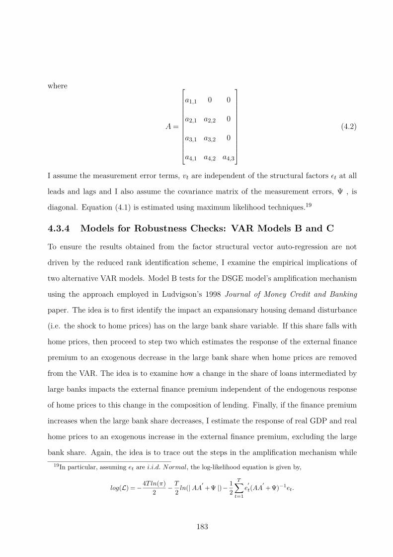
where

A=

a1,1 0 0

a2,1 a2,2 0

a3,1 a3,2 0

a4,1 a4,2 a4,3

(4.2)

I assume the measurement error terms, vt are independent of the structural factors ǫt at all

leads and lags and I also assume the covariance matrix of the measurement errors, Ψ , is

diagonal. Equation (4.1) is estimated using maximum likelihood techniques.19

4.3.4 Models for Robustness Checks: VAR Models B and C

To ensure the results obtained from the factor structural vector auto-regression are not

driven by the reduced rank identification scheme, I examine the empirical implications of

two alternative VAR models. Model B tests for the DSGE model’s amplification mechanism

using the approach employed in Ludvigson’s 1998 Journal of Money Credit and Banking

paper. The idea is to first identify the impact an expansionary housing demand disturbance

(i.e. the shock to home prices) has on the large bank share variable. If this share falls with

home prices, then proceed to step two which estimates the response of the external finance

premium to an exogenous decrease in the large bank share when home prices are removed

from the VAR. The idea is to examine how a change in the share of loans intermediated by

large banks impacts the external finance premium independent of the endogenous response

of home prices to this change in the composition of lending. Finally, if the finance premium

increases when the large bank share decreases, I estimate the response of real GDP and real

home prices to an exogenous increase in the external finance premium, excluding the large

bank share. Again, the idea is to trace out the steps in the amplification mechanism while

19In particular, assuming et are i.i.d. Normal, the log-likelihood equation is given by,

log(L) = −4T ln(π)

2− T

2ln(|AA′

+Ψ |)− 1

2

T∑

t=1

e′

t(AA′

+Ψ)−1et.

183

controlling for the endogenous reaction of home prices and the share of credit held by large

banks respectively.

Model C takes this idea one step further and estimates a series of bivariate VARs. The first

VAR has home prices and the large bank share. If falling home prices causes large banks

to withdraw relatively more credit than smaller banks, then I estimate a second bivariate

VAR which includes the external finance premium and the share of credit held by large

banks. If reductions in the large bank share drive-up finance premiums, then I estimate a

third bivariate VAR with the external finance premium and GDP. If this VAr indicates that

rising finance premiums causes real GDP to fall, then this provides evidence in support of

the equilibrium model’s amplification mechanism spelled out in Section (4.3.1). T

Throughout all of these VAR models, I order variables as follows: the external finance

premium, real GDP, real home prices and the large bank share. The motivation for this

ordering follows from the equilibrium model’s impulse response functions in Figure (4.2).

The most delicate issue of this ordering lies in the decision of whether to place real GDP

before real home prices or vis-a-versa. The equilibrium model implies both have a non-

zero response to housing demand and technology shocks. Fortunately all the results for the

recursive models used in Model B and Model C are robust to reversing the ordering of real

GDP and real home prices. Model A treats both of these variables symmetrically and for

this reason is the preferred model.

4.3.5 Model A: IRFs

Impulse response functions trace out the path of the variables in periods t = 0,1,2, ... in

response to a one time structural disturbance in period t= 0. Confidence bands are computed

using Monte Carlo integration techniques assuming a normal likelihood and uninformative

prior.

In order to test the model’s amplification prediction the first step is to examine if a drop in

home prices caused by an aggregate downturn tightens the large banks’ moral hazard con-

184

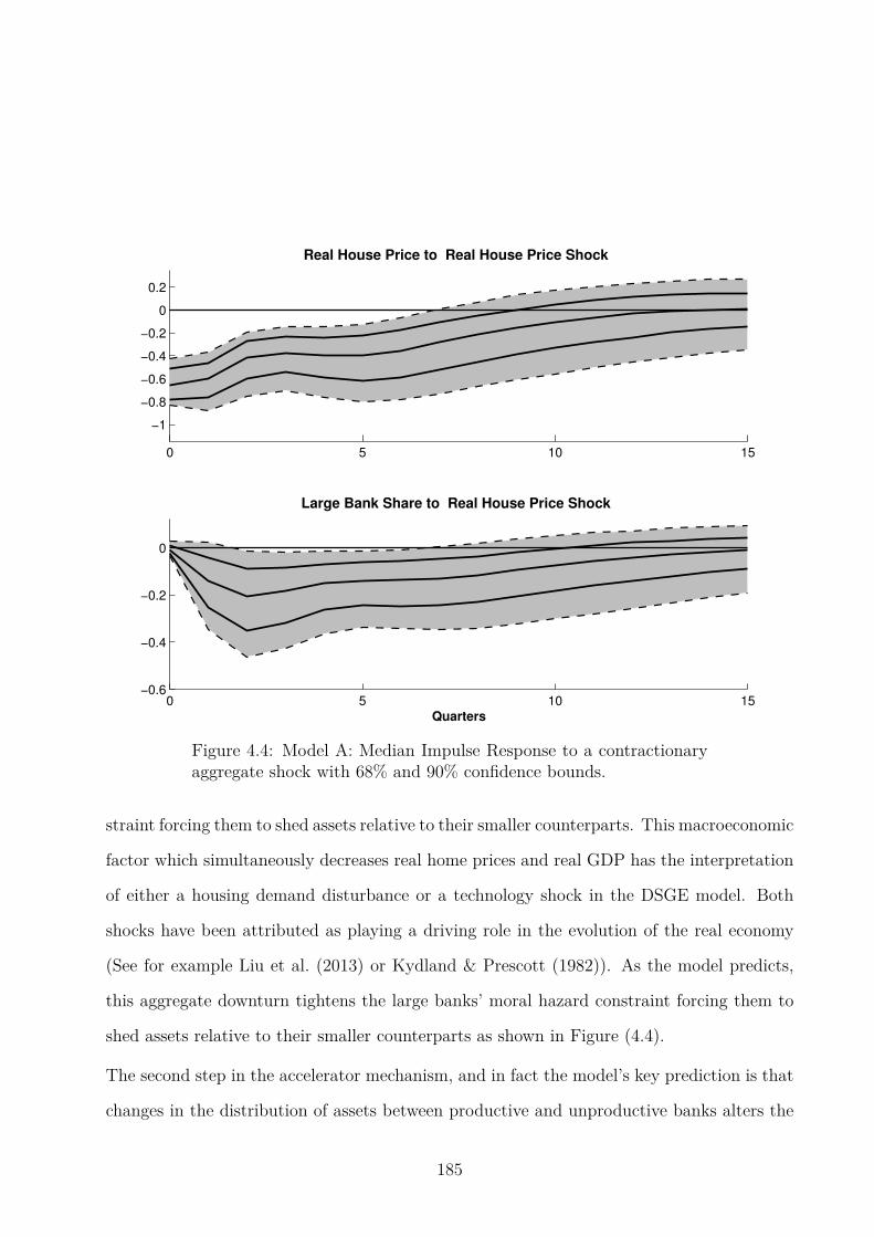
0 5 10 15

−1

−0.8

−0.6

−0.4

−0.2

0

0.2

Real House Price to Real House Price Shock

0 5 10 15−0.6

−0.4

−0.2

0

Quarters

Large Bank Share to Real House Price Shock

Figure 4.4: Model A: Median Impulse Response to a contractionaryaggregate shock with 68% and 90% confidence bounds.

straint forcing them to shed assets relative to their smaller counterparts. This macroeconomic

factor which simultaneously decreases real home prices and real GDP has the interpretation

of either a housing demand disturbance or a technology shock in the DSGE model. Both

shocks have been attributed as playing a driving role in the evolution of the real economy

(See for example Liu et al. (2013) or Kydland & Prescott (1982)). As the model predicts,

this aggregate downturn tightens the large banks’ moral hazard constraint forcing them to

shed assets relative to their smaller counterparts as shown in Figure (4.4).

The second step in the accelerator mechanism, and in fact the model’s key prediction is that

changes in the distribution of assets between productive and unproductive banks alters the

185

0 5 10 15

−1

−0.8

−0.6

−0.4

−0.2

0

Quarters

Large Bank Share to Large Bank Share Shock

0 5 10 15

−2

0

2

4

6

EFP to Large Bank Share Shock

Figure 4.5: Model A: Median Impulse Response to an exogenousdecrease in the large bank share with 68% and 90% confidence bounds.

finance terms offered to borrowers. For example, if the assets shift to less productive banks,

which are the small banks in equilibrium, finance premiums will rise as the liquid value of

the borrowers collateral falls when it is held by these unproductive intermediaries. The data

confirms this prediction in Figure (4.5). An exogenous decrease in the share of assets held

by large banks increases the external finance premium, suggesting financing conditions are

worsening.

Since the VAR has confirmed the first two steps of the accelerator mechanism, I proceed to

the third step to examine how rising finance premiums affect the macroeconomy. In partic-

ular, the model predicts that rising financing costs will lead to an increase in defaults and

ultimately lower home price due to the increased supply of homes on the market. Moreover,

186

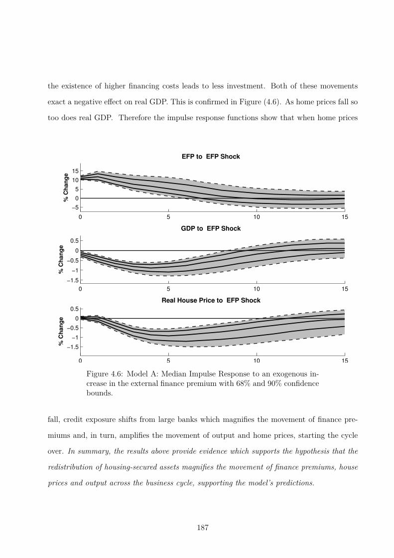
the existence of higher financing costs leads to less investment. Both of these movements

exact a negative effect on real GDP. This is confirmed in Figure (4.6). As home prices fall so

too does real GDP. Therefore the impulse response functions show that when home prices

0 5 10 15

−5

0

5

10

15

% C

han

ge

EFP to EFP Shock

0 5 10 15

−1.5

−1

−0.5

0

0.5

% C

han

ge

GDP to EFP Shock

0 5 10 15

−1.5

−1

−0.5

0

0.5

% C

han

ge

Real House Price to EFP Shock

Figure 4.6: Model A: Median Impulse Response to an exogenous in-crease in the external finance premium with 68% and 90% confidencebounds.

fall, credit exposure shifts from large banks which magnifies the movement of finance pre-

miums and, in turn, amplifies the movement of output and home prices, starting the cycle

over. In summary, the results above provide evidence which supports the hypothesis that the

redistribution of housing-secured assets magnifies the movement of finance premiums, house

prices and output across the business cycle, supporting the model’s predictions.

187

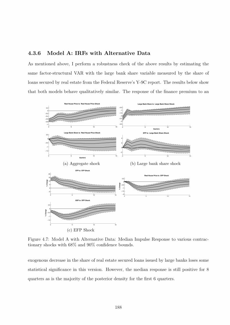
4.3.6 Model A: IRFs with Alternative Data

As mentioned above, I perform a robustness check of the above results by estimating the

same factor-structural VAR with the large bank share variable measured by the share of

loans secured by real estate from the Federal Reserve’s Y-9C report. The results below show

that both models behave qualitatively similar. The response of the finance premium to an

0 5 10 15

−1

−0.8

−0.6

−0.4

−0.2

0

0.2

Real House Price to Real House Price Shock

0 5 10 15

−1.5

−1

−0.5

0

0.5

Quarters

Large Bank Share to Real House Price Shock

(a) Aggregate shock

0 5 10 15

−3.5

−3

−2.5

−2

−1.5

−1

−0.5

Quarters

Large Bank Share to Large Bank Share Shock

0 5 10 15

−2

0

2

4

EFP to Large Bank Share Shock

(b) Large bank share shock

0 5 10 15

−5

0

5

10

15

20

% C

ha

ng

e

EFP to EFP Shock

0 5 10 15

−1.5

−1

−0.5

0

0.5

% C

ha

ng

e

GDP to EFP Shock

(c) EFP Shock

0 5 10 15

−2

−1.5

−1

−0.5

0

0.5

% C

ha

ng

e

Real House Price to EFP Shock

Figure 4.7: Model A with Alternative Data: Median Impulse Response to various contrac-tionary shocks with 68% and 90% confidence bounds.

exogenous decrease in the share of real estate secured loans issued by large banks loses some

statistical significance in this version. However, the median response is still positive for 8

quarters as is the majority of the posterior density for the first 6 quarters.

188

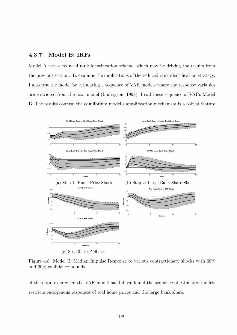
4.3.7 Model B: IRFs

Model A uses a reduced rank identification scheme, which may be driving the results from

the previous section. To examine the implications of the reduced rank identification strategy,

I also test the model by estimating a sequence of VAR models where the response variables

are restricted from the next model (Ludvigson, 1998). I call these sequence of VARs Model

B. The results confirm the equilibrium model’s amplification mechanism is a robust feature

0 5 10 15

−1

−0.5

0

Real House Price to Real House Price Shock

0 5 10 15−0.6

−0.4

−0.2

0

0.2

Quarters

Large Bank Share to Real House Price Shock

(a) Step 1: Home Price Shock

0 5 10 15

−1

−0.8

−0.6

−0.4

−0.2

0

Large Bank Share to Large Bank Share Shock

0 5 10 15

−2

0

2

4

6

Quarters

EFP to Large Bank Share Shock

(b) Step 2: Large Bank Share Shock

0 5 10 15

−5

0

5

10

15

20

% C

ha

ng

e

EFP to EFP Shock

0 5 10 15

−1.5

−1

−0.5

0

0.5

% C

ha

ng

e

Quarters

GDP to EFP Shock

(c) Step 3: EFP Shock

0 5 10 15

−1.5

−1

−0.5

0

0.5

% C

ha

ng

e

Quarters

Real House Price to EFP Shock

Figure 4.8: Model B: Median Impulse Response to various contractionary shocks with 68%and 90% confidence bounds.

of the data, even when the VAR model has full rank and the sequence of estimated models

restricts endogenous responses of real home prices and the large bank share.

189

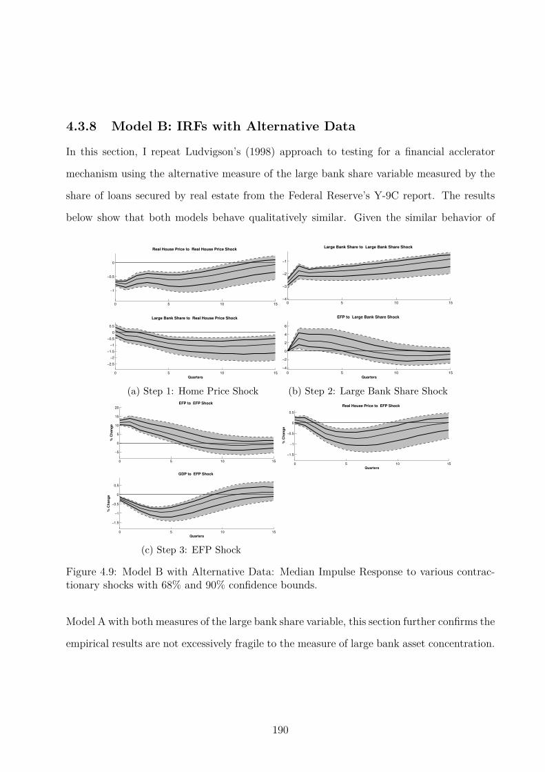
4.3.8 Model B: IRFs with Alternative Data

In this section, I repeat Ludvigson’s (1998) approach to testing for a financial acclerator

mechanism using the alternative measure of the large bank share variable measured by the

share of loans secured by real estate from the Federal Reserve’s Y-9C report. The results

below show that both models behave qualitatively similar. Given the similar behavior of

0 5 10 15

−1

−0.5

0

Real House Price to Real House Price Shock

0 5 10 15

−2.5

−2

−1.5

−1

−0.5

0

0.5

Quarters

Large Bank Share to Real House Price Shock

(a) Step 1: Home Price Shock

0 5 10 15−4

−3

−2

−1

Large Bank Share to Large Bank Share Shock

0 5 10 15

−4

−2

0

2

4

6

Quarters

EFP to Large Bank Share Shock

(b) Step 2: Large Bank Share Shock

0 5 10 15

−5

0

5

10

15

20

% C

ha

ng

e

EFP to EFP Shock

0 5 10 15

−1.5

−1

−0.5

0

0.5

% C

ha

ng

e

Quarters

GDP to EFP Shock

(c) Step 3: EFP Shock

0 5 10 15

−1.5

−1

−0.5

0

0.5

% C

ha

ng

e

Quarters

Real House Price to EFP Shock

Figure 4.9: Model B with Alternative Data: Median Impulse Response to various contrac-tionary shocks with 68% and 90% confidence bounds.

Model A with both measures of the large bank share variable, this section further confirms the

empirical results are not excessively fragile to the measure of large bank asset concentration.

190

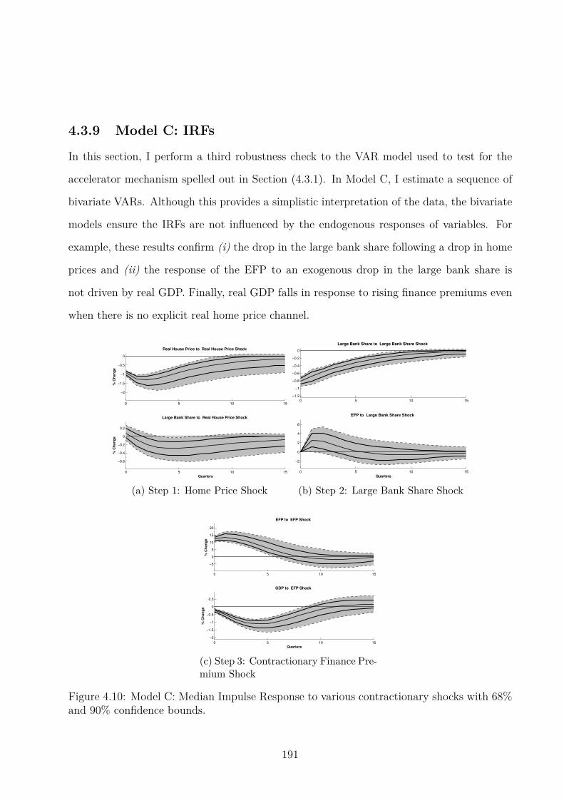
4.3.9 Model C: IRFs

In this section, I perform a third robustness check to the VAR model used to test for the

accelerator mechanism spelled out in Section (4.3.1). In Model C, I estimate a sequence of

bivariate VARs. Although this provides a simplistic interpretation of the data, the bivariate

models ensure the IRFs are not influenced by the endogenous responses of variables. For

example, these results confirm (i) the drop in the large bank share following a drop in home

prices and (ii) the response of the EFP to an exogenous drop in the large bank share is

not driven by real GDP. Finally, real GDP falls in response to rising finance premiums even

when there is no explicit real home price channel.

0 5 10 15

−2

−1.5

−1

−0.5

0

% C

ha

ng

e

Real House Price to Real House Price Shock

0 5 10 15

−0.6

−0.4

−0.2

0

0.2

% C

ha

ng

e

Quarters

Large Bank Share to Real House Price Shock

(a) Step 1: Home Price Shock

0 5 10 15

−1.2

−1

−0.8

−0.6

−0.4

−0.2

0

Large Bank Share to Large Bank Share Shock

0 5 10 15

−2

0

2

4

6

Quarters

EFP to Large Bank Share Shock

(b) Step 2: Large Bank Share Shock

0 5 10 15

−5

0

5

10

15

20

% C

ha

ng

e

EFP to EFP Shock

0 5 10 15

−2

−1.5

−1

−0.5

0

0.5

% C

ha

ng

e

Quarters

GDP to EFP Shock

(c) Step 3: Contractionary Finance Pre-mium Shock

Figure 4.10: Model C: Median Impulse Response to various contractionary shocks with 68%and 90% confidence bounds.

191

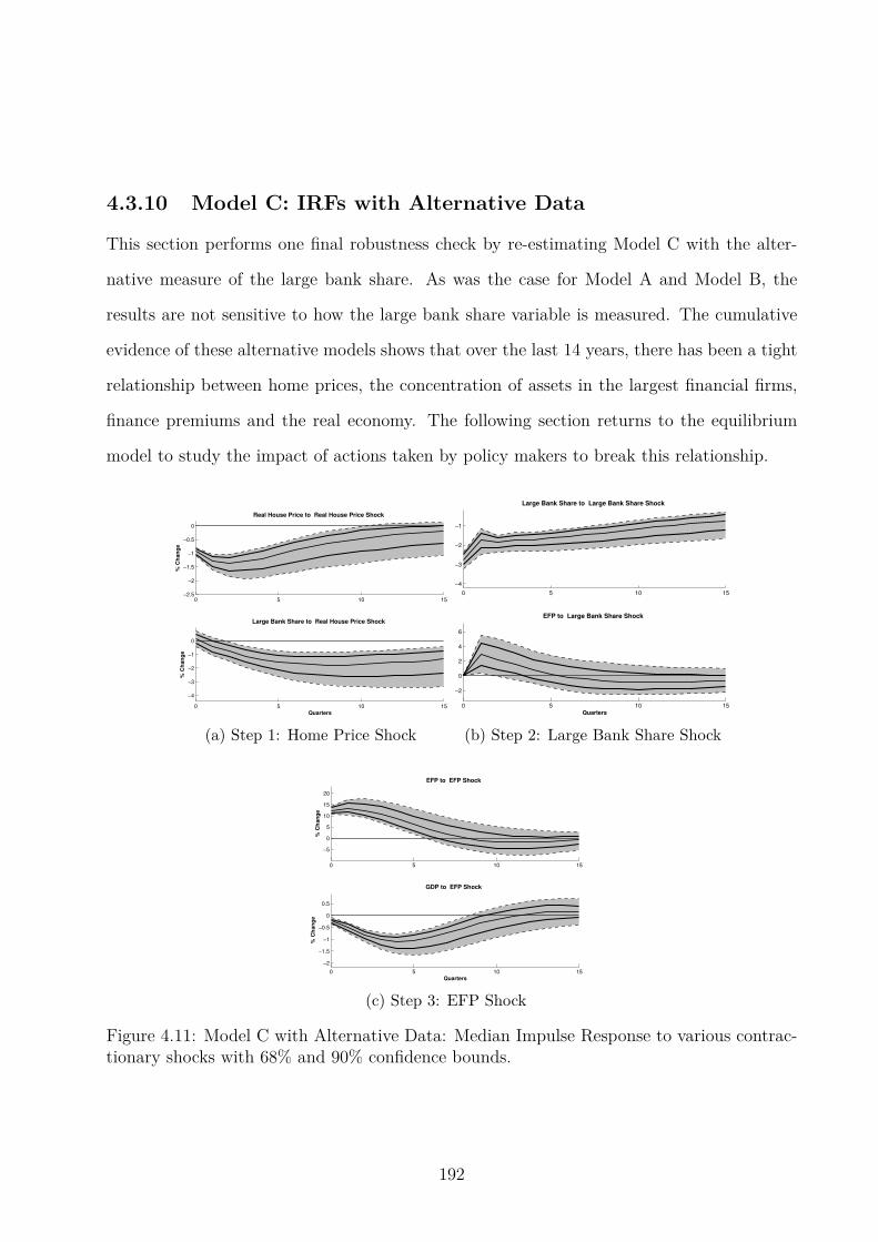
4.3.10 Model C: IRFs with Alternative Data

This section performs one final robustness check by re-estimating Model C with the alter-

native measure of the large bank share. As was the case for Model A and Model B, the

results are not sensitive to how the large bank share variable is measured. The cumulative

evidence of these alternative models shows that over the last 14 years, there has been a tight

relationship between home prices, the concentration of assets in the largest financial firms,

finance premiums and the real economy. The following section returns to the equilibrium

model to study the impact of actions taken by policy makers to break this relationship.

0 5 10 15−2.5

−2

−1.5

−1

−0.5

0

% C

ha

ng

e

Real House Price to Real House Price Shock

0 5 10 15

−4

−3

−2

−1

0

% C

ha

ng

e

Quarters

Large Bank Share to Real House Price Shock

(a) Step 1: Home Price Shock

0 5 10 15

−4

−3

−2

−1

Large Bank Share to Large Bank Share Shock

0 5 10 15

−2

0

2

4

6

Quarters

EFP to Large Bank Share Shock

(b) Step 2: Large Bank Share Shock

0 5 10 15

−5

0

5

10

15

20

% C

ha

ng

e

EFP to EFP Shock

0 5 10 15

−2

−1.5

−1

−0.5

0

0.5

% C

ha

ng

e

Quarters

GDP to EFP Shock

(c) Step 3: EFP Shock

Figure 4.11: Model C with Alternative Data: Median Impulse Response to various contrac-tionary shocks with 68% and 90% confidence bounds.

192

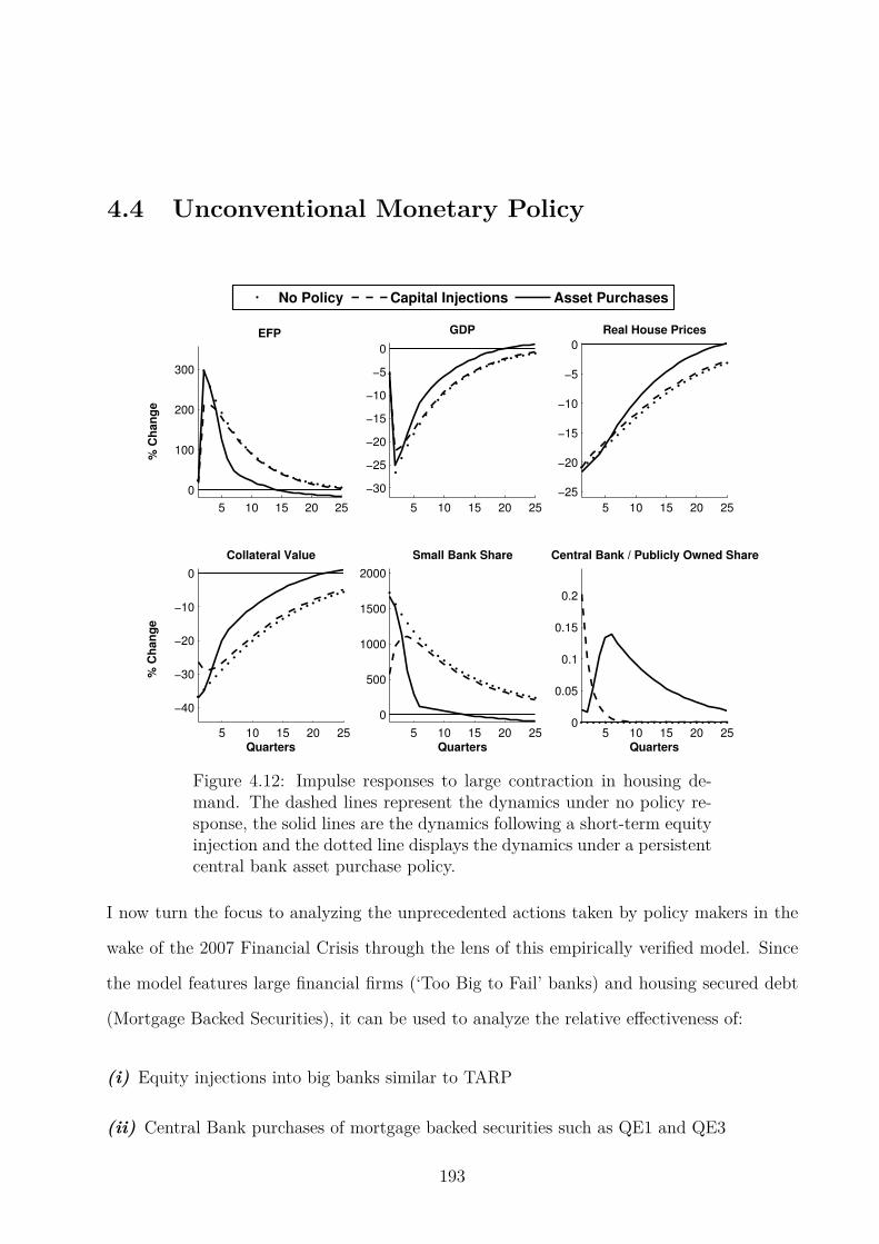
4.4 Unconventional Monetary Policy

5 10 15 20 25

0

100

200

300

% C

han

ge

EFP

No Policy Capital Injections Asset Purchases

5 10 15 20 25

−30

−25

−20

−15

−10

−5

0

GDP

5 10 15 20 25

−25

−20

−15

−10

−5

0

Real House Prices

5 10 15 20 25

−40

−30

−20

−10

0

% C

han

ge

Quarters

Collateral Value

5 10 15 20 25

0

500

1000

1500

2000

Quarters

Small Bank Share

5 10 15 20 250

0.05

0.1

0.15

0.2

Quarters

Central Bank / Publicly Owned Share

Figure 4.12: Impulse responses to large contraction in housing de-mand. The dashed lines represent the dynamics under no policy re-sponse, the solid lines are the dynamics following a short-term equityinjection and the dotted line displays the dynamics under a persistentcentral bank asset purchase policy.

I now turn the focus to analyzing the unprecedented actions taken by policy makers in the

wake of the 2007 Financial Crisis through the lens of this empirically verified model. Since

the model features large financial firms (‘Too Big to Fail’ banks) and housing secured debt

(Mortgage Backed Securities), it can be used to analyze the relative effectiveness of:

(i) Equity injections into big banks similar to TARP

(ii) Central Bank purchases of mortgage backed securities such as QE1 and QE3

193

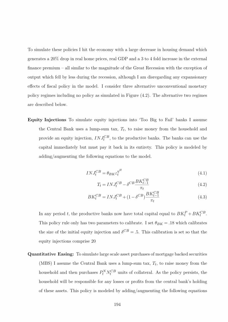
To simulate these policies I hit the economy with a large decrease in housing demand which

generates a 20% drop in real home prices, real GDP and a 3 to 4 fold increase in the external

finance premium – all similar to the magnitude of the Great Recession with the exception of

output which fell by less during the recession, although I am disregarding any expansionary

effects of fiscal policy in the model. I consider three alternative unconventional monetary

policy regimes including no policy as simulated in Figure (4.2). The alternative two regimes

are described below.

Equity Injections To simulate equity injections into ‘Too Big to Fail’ banks I assume

the Central Bank uses a lump-sum tax, Tt, to raise money from the household and

provide an equity injection, INJCBt , to the productive banks. The banks can use the

capital immediately but must pay it back in its entirety. This policy is modeled by

adding/augmenting the following equations to the model.

INJCBt = θBKεηH

t (4.1)

Tt = INJCBt − δCBBKCB

t−1

πt(4.2)

BKCBt = INJCBt +(1− δCB)

BKCBt−1

πt(4.3)

In any period t, the productive banks now have total capital equal to BKPt +BKCB

t .

This policy rule only has two parameters to calibrate. I set θBK = .18 which calibrates

the size of the initial equity injection and δCB = .5. This calibration is set so that the

equity injections comprise 20

Quantitative Easing: To simulate large scale asset purchases of mortgage backed securities

(MBS) I assume the Central Bank uses a lump-sum tax, Tt, to raise money from the

household and then purchases PNt NCBt units of collateral. As the policy persists, the

household will be responsible for any losses or profits from the central bank’s holding

of these assets. This policy is modeled by adding/augmenting the following equations

194

to the model.

NCBt = ρNNCB

t−1 +4∑

j=0

θNj εηH

t−j (4.4)

Tt = PNt NCBt − (1−Ft−1(ωt))p

Nt−1N

CBt−1r

Dt−1 −Ft−1(ωt)P

Ht Z

RNCBt−1 (4.5)

In any period t, the market clearing condition for secured lending is now given by,

N = νNUt +(1−ν)NP

t +NCBt . (4.6)

This policy rule has six parameters to calibrate. I set θN0 = θN4 = .5, θN1 = θN3 = 1 and

θN2 = 1.4 which calibrates the flow of central bank asset purchases to have a hump-

shaped pattern with the flow of purchases of Mortgage-Backed Securities held outright

by the central bank (using data from the Flow of Funds H.4.1, Factors Affecting Reserve

Balances) peaking at 14% of the total credit exposure of all commercial banks. 20 and

I set ρN = .9 to capture the prolonged nature of the Quantitative Easing policies

implemented by the Federal Reserve. In particular, with ρN = .9 the purchases last for

more than 8 years. In the welfare section I vary this.

Equity Injections vs. Quantitative Easing

The simulations of the large fall in housing demand are illustrated in Figure (4.12) under all

three unconventional policy regimes – including no policy intervention. The results reveal

that both equity injections and large-scale asset purchases (LSAP’s) mitigate the crisis on

impact. However, the duration of the unconventional policies plays a critical role in de-

termining the time it takes to recover from the recession. Since the equity injections are

paid back after 7 quarters, the dynamics under this regime converge towards the no-policy

regime. The length of the recession is essentially unchanged – although the initial severity is

20Credit exposure is computed as explained in Section (4.3.2) using data from the OCC’s QuarterlyDerivatives Reports

195

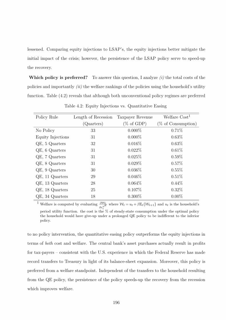
lessened. Comparing equity injections to LSAP’s, the equity injections better mitigate the

initial impact of the crisis; however, the persistence of the LSAP policy serve to speed-up

the recovery.

Which policy is preferred? To answer this question, I analyze (i) the total costs of the

policies and importantly (ii) the welfare rankings of the policies using the household’s utility

function. Table (4.2) reveals that although both unconventional policy regimes are preferred

Table 4.2: Equity Injections vs. Quantitative Easing

Policy Rule Length of Recession Taxpayer Revenue Welfare Cost1

(Quarters) (% of GDP) (% of Consumption)

No Policy 33 0.000% 0.71%

Equity Injections 31 0.000% 0.63%

QE, 5 Quarters 32 0.016% 0.63%

QE, 6 Quarters 31 0.022% 0.61%

QE, 7 Quarters 31 0.025% 0.59%

QE, 8 Quarters 31 0.029% 0.57%

QE, 9 Quarters 30 0.036% 0.55%

QE, 11 Quarters 29 0.046% 0.51%

QE, 13 Quarters 28 0.064% 0.44%

QE, 18 Quarters 25 0.107% 0.32%

QE, 34 Quarters 18 0.300% 0.00%

1 Welfare is computed by evaluating ∂Wt

∂εηH

t

where Wt = ut +βEtWt+1 and ut is the household’s

period utility function. the cost is the % of steady-state consumption under the optimal policythe household would have give-up under a prolonged QE policy to be indifferent to the inferiorpolicy.

to no policy intervention, the quantitative easing policy outperforms the equity injections in

terms of both cost and welfare. The central bank’s asset purchases actually result in profits

for tax-payers – consistent with the U.S. experience in which the Federal Reserve has made

record transfers to Treasury in light of its balance-sheet expansion. Moreover, this policy is

preferred from a welfare standpoint. Independent of the transfers to the household resulting

from the QE policy, the persistence of the policy speeds-up the recovery from the recession

which improves welfare.

196

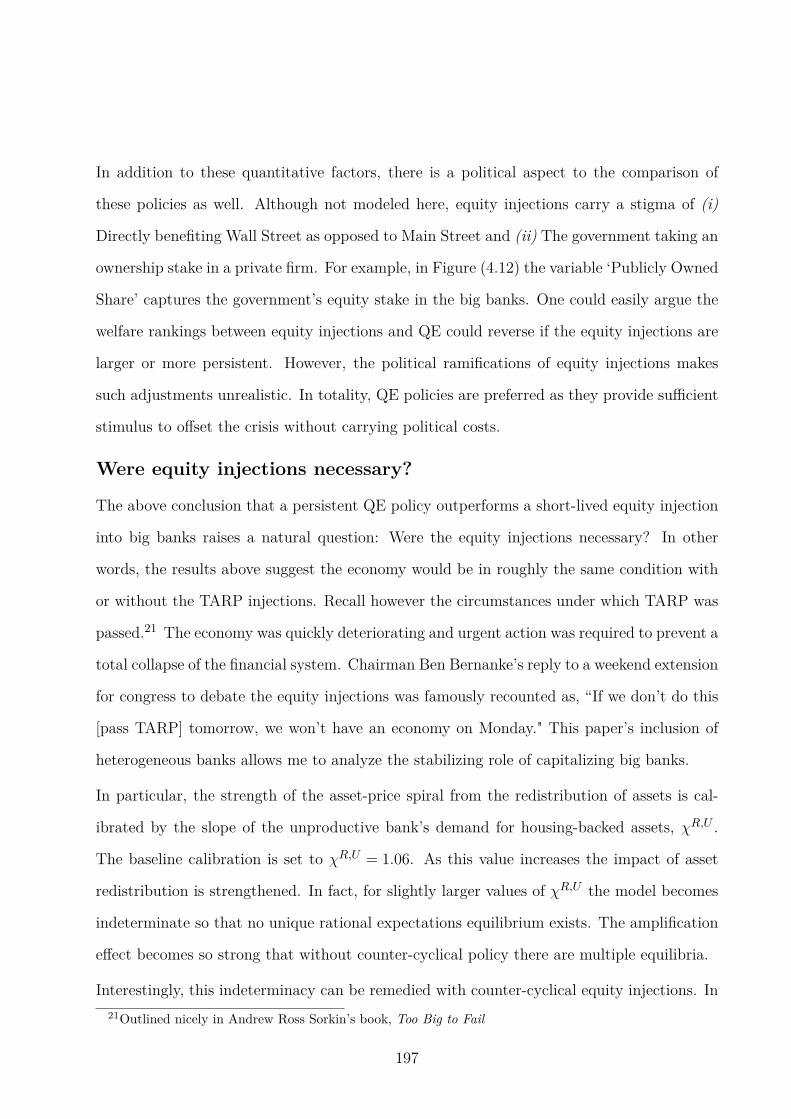
In addition to these quantitative factors, there is a political aspect to the comparison of

these policies as well. Although not modeled here, equity injections carry a stigma of (i)

Directly benefiting Wall Street as opposed to Main Street and (ii) The government taking an

ownership stake in a private firm. For example, in Figure (4.12) the variable ‘Publicly Owned

Share’ captures the government’s equity stake in the big banks. One could easily argue the

welfare rankings between equity injections and QE could reverse if the equity injections are

larger or more persistent. However, the political ramifications of equity injections makes

such adjustments unrealistic. In totality, QE policies are preferred as they provide sufficient

stimulus to offset the crisis without carrying political costs.

Were equity injections necessary?

The above conclusion that a persistent QE policy outperforms a short-lived equity injection

into big banks raises a natural question: Were the equity injections necessary? In other

words, the results above suggest the economy would be in roughly the same condition with

or without the TARP injections. Recall however the circumstances under which TARP was

passed.21 The economy was quickly deteriorating and urgent action was required to prevent a

total collapse of the financial system. Chairman Ben Bernanke’s reply to a weekend extension

for congress to debate the equity injections was famously recounted as, “If we don’t do this

[pass TARP] tomorrow, we won’t have an economy on Monday." This paper’s inclusion of

heterogeneous banks allows me to analyze the stabilizing role of capitalizing big banks.

In particular, the strength of the asset-price spiral from the redistribution of assets is cal-

ibrated by the slope of the unproductive bank’s demand for housing-backed assets, χR,U .

The baseline calibration is set to χR,U = 1.06. As this value increases the impact of asset

redistribution is strengthened. In fact, for slightly larger values of χR,U the model becomes

indeterminate so that no unique rational expectations equilibrium exists. The amplification

effect becomes so strong that without counter-cyclical policy there are multiple equilibria.

Interestingly, this indeterminacy can be remedied with counter-cyclical equity injections. In

21Outlined nicely in Andrew Ross Sorkin’s book, Too Big to Fail

197

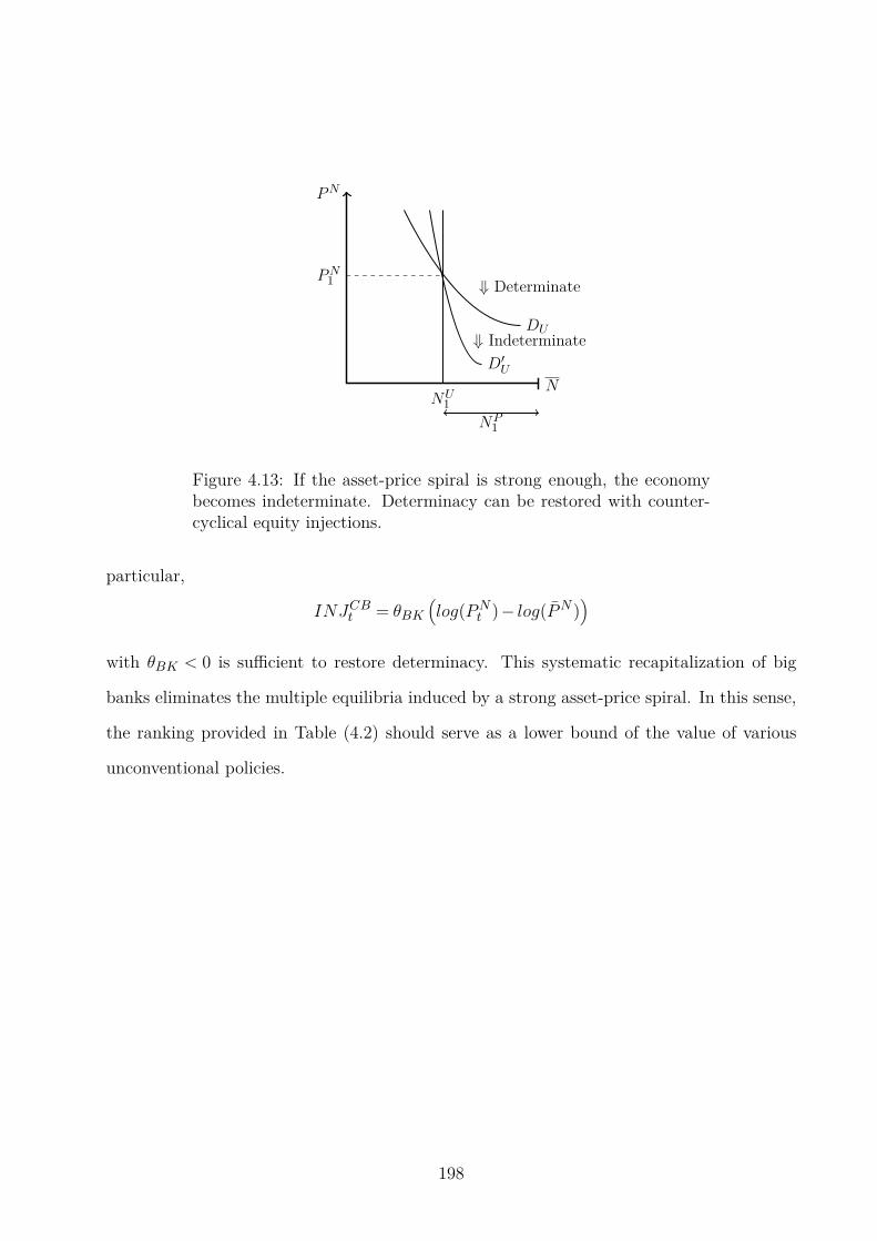
N

PN

NU1

NP1

DU

PN1

D′U

⇓ Indeterminate

⇓ Determinate

Figure 4.13: If the asset-price spiral is strong enough, the economybecomes indeterminate. Determinacy can be restored with counter-cyclical equity injections.

particular,

INJCBt = θBK(

log(PNt )− log(PN ))

with θBK < 0 is sufficient to restore determinacy. This systematic recapitalization of big

banks eliminates the multiple equilibria induced by a strong asset-price spiral. In this sense,

the ranking provided in Table (4.2) should serve as a lower bound of the value of various

unconventional policies.

198

4.5 Conclusion

The paper presents a financial mechanism which is able to capture salient features of the

U.S. economy stemming from the interconnectedness of housing and financial markets. The

interaction between the two sectors allows for a more natural interpretation of what set-off the

Great Recession, a drop in housing demand, as opposed to the “Financial Shocks” that other

papers consider. Beyond simply being the source of the initial downturn, the housing market

also plays a fundamental role in prolonging the downturn. Since housing is a durable, when

defaults begin rising due to a drop in home prices, the future price of housing will remain

depressed as it takes time for the stock of homes to return to normal levels. This mechanism

captures the observed empirical relationship between the external finance premium and home

prices, output and investment; a relationship which the traditional Bernanke et al. (1999)

financial accelerator fails to capture.

In addition to integrating housing and financial markets, in this paper I provide insights

for policy makers regarding the treatment of “Too Big to Fail” banks. By eschewing the

assumption that all banks are the same (or similarly, banks face no agency problems), I am

able to show why big banks withdrew relatively more credit during the Great Recession.

The model’s qualitative predictions for the joint behavior of the asset concentration in large

banks, home prices, output and finance premiums are confirmed using an estimated VAR.

Beyond capturing this empirical observation, the model shows the differential behavior be-

tween big banks and their smaller counter parts served to strengthen the Great Recession.

Therefore, the equity injections into the largest financial firms in 2008 are well justified as

they mitigated the severity of the downturn and prevented a potential collapse. Although

this thwarted the initial downturn, policies such as “QE 1/3,” the Fed’s Mortgage Backed

Security purchase programs, play an important role in the model by speeding up the recovery.

199

Future Work

Although this paper explains why big banks withdrew relatively more credit when home

prices plunged in 2007 and provides a transmission channel for unconventional monetary

policy, much work lies ahead. In particular, the policy options in this paper are designed

to clean-up after the crash instead of preventing it in the first place. Moving beyond crisis

management, the empirically validated financial structure presented in this paper can be

used to explore the efficacy of macroprudential policy in preventing a build-up of assets in

large financial firms when home prices rise.

A question of empirical importance arises as well from the model. Christiano et al. (2013)

show that “risk shocks” have played a substantial role in shaping the business cycle for the

last 20 years. However, they point out their finding is driven by the ability of risk shocks to

generate the empirical observation that credit contracts during recessions. Due to the novel

debt contract I introduce in this paper, credit contracts following adverse technology and

demand shocks – the usual business cycle suspects. Given the policy implications, it is worth

while to examine the robustness of their results in this housing-centered financial structure.

200

References

Adrian, T. & Shin, H. S. (2010). Financial intermediaries and monetary economics. In

B. M. Friedman & M. Woodford (Eds.), Handbook of Monetary Economics, volume 3 of

Handbook of Monetary Economics chapter 12, (pp. 601–650). Elsevier.

Anderson, T. (2003). An introduction to multivariate statistical analysis. Wiley series in

probability and mathematical statistics. Probability and mathematical statistics. Wiley.

Anderson, T. W. & Rubin, H. (1956). Statistical inference in factor analysis. In Proceedings

of the third Berkeley symposium on mathematical statistics and probability, volume 5 (pp.

1–1).

Bernanke, B. S., Gertler, M., & Gilchrist, S. (1999). The financial accelerator in a quan-

titative business cycle framework. In J. B. Taylor & M. Woodford (Eds.), Handbook of

Macroeconomics, volume 1 of Handbook of Macroeconomics chapter 21, (pp. 1341–1393).

Elsevier.

Blanchard, O. J. & Quah, D. (1989). The dynamic effects of aggregate demand and supply

disturbances. American Economic Review, 79(4), 655–73.

Bos, J. W. & Kolari, J. W. (2013). Optimal size in banking, (pp. 77–94). John Wiley &

Sons, Ltd.

Breuer, P. (2000). Measuring off-balance-sheet leverage. IMF Working Paper.

201

Carlstrom, C. T. & Fuerst, T. S. (1997). Agency costs, net worth, and business fluctuations:

A computable general equilibrium analysis. American Economic Review, 87(5), 893–910.

Carlstrom, C. T., Fuerst, T. S., Ortiz, A., & Paustian, M. (2012). Estimating contract

indexation in a financial accelerator model. Technical report.

Christiano, L., Motto, R., & Rostagno, M. (2013). Risk Shocks. NBER Working Papers

18682, National Bureau of Economic Research, Inc.

Christiano, L. J., Eichenbaum, M., & Evans, C. L. (2005). Nominal rigidities and the dynamic

effects of a shock to monetary policy. Journal of Political Economy, 113(1), 1–45.

Davis, M. A. & Heathcote, J. (2005). Housing and the business cycle. International Economic

Review, 46(3), 751–784.

Demirguc-Kunt, A., Detragiache, E., & Merrouche, O. (2013). Bank capital: Lessons from

the financial crisis. Journal of Money, Credit and Banking, 45(6), 1147–1164.

Gerali, A., Neri, S., Sessa, L., & Signoretti, F. M. (2010). Credit and banking in a dsge

model of the euro area. Journal of Money, Credit and Banking, 42(s1), 107–141.

Gertler, M. & Karadi, P. (2011). A model of unconventional monetary policy. Journal of

Monetary Economics, 58(1), 17–34.

Gertler, M. & Kiyotaki, N. (2010). Financial intermediation and credit policy in business cy-

cle analysis. In B. M. Friedman & M. Woodford (Eds.), Handbook of Monetary Economics,

volume 3 of Handbook of Monetary Economics chapter 11, (pp. 547–599). Elsevier.

Gorodnichenko, Y. (2005). Reduced-Rank Identification of Structural Shocks in VARs.

Macroeconomics 0512011, EconWPA.

Hafstead, M. & Smith, J. (2012). Financial shocks, bank intermediation, and monetary

policy in a dsge model. Unpublished Manucript.

202

Iacoviello, M. (2005). House prices, borrowing constraints, and monetary policy in the

business cycle. American Economic Review, 95(3), 739–764.

Iacoviello, M. & Neri, S. (2010). Housing market spillovers: Evidence from an estimated

dsge model. American Economic Journal: Macroeconomics, 2(2), 125–64.

Kiyotaki, N. & Moore, J. (1997). Credit cycles. Journal of Political Economy, 105(2), 211–48.

Kydland, F. E. & Prescott, E. C. (1982). Time to build and aggregate fluctuations. Econo-

metrica, 50(6), 1345–70.

Liu, Z., Wang, P., & Zha, T. (2013). Land-price dynamics and macroeconomic fluctuations.

Econometrica, 81(3), 1147–1184.

Ludvigson, S. (1998). The channel of monetary transmission to demand: evidence from the

market for automobile credit. Journal of Money, Credit and Banking, (pp. 365–383).

Oulton, N. & Rincon-Aznar, A. (2009). Rates of Return and Alternative Measures of Capital

Input: 14 Countries and 10 Branches, 1971-2005. Cep discussion papers, Centre for

Economic Performance, LSE.

Shen, G. (2011). News shocks and the external finance premium. The B.E. Journal of

Macroeconomics, 11(1), 1–27.

Townsend, R. M. (1979). Optimal contracts and competitive markets with costly state

verification. Journal of Economic Theory, 21(2), 265–293.

Wheelock, D. C. & Wilson, P. W. (2012). Do large banks have lower costs? new estimates

of returns to scale for u.s. banks. Journal of Money, Credit and Banking, 44(1), 171–199.

203

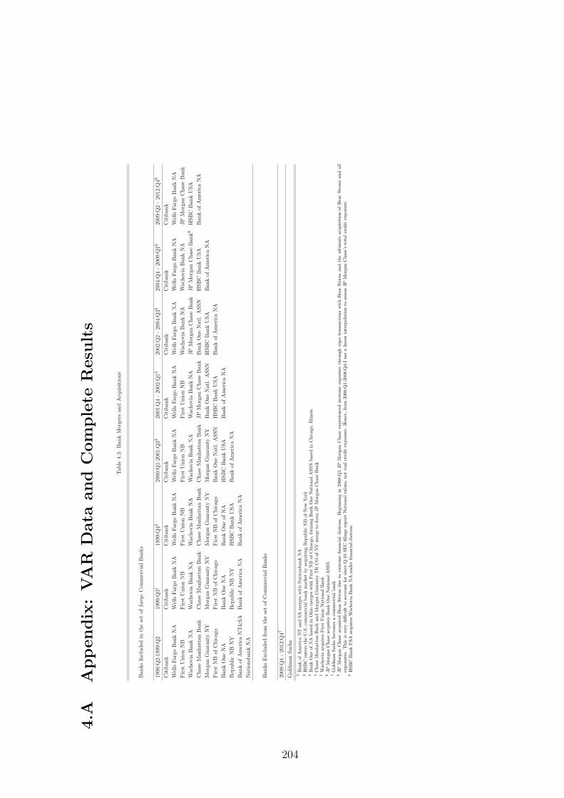
4.A

Ap

pen

dix

:V

AR

Data

an

dC

om

ple

teR

esu

lts

Tab

le4.

3:B

ank

Mer

gers

and

Acq

uis

itio

ns

Ban

ks

Incl

uded

inth

ese

tof

Lar

geC

omm

erci

alB

anks

1998

:Q2-

1999

:Q2

1999

:Q31

1999

:Q42

2000

:Q1-

2001

:Q33

2001

:Q4

-20

02:Q

1420

02:Q

2-

2004

:Q35

2004

:Q4

-20

09:Q

1620

09:Q

2-

2012

:Q49

Cit

iban

kC

itib

ank

Cit

iban

kC

itib

ank

Cit

iban

kC

itib

ank

Cit

iban

kC

itib

ank

Wel

lsFar

goB

ank

NA

Wel

lsFar

goB

ank

NA

Wel

lsFar

goB

ank

NA

Wel

lsFar

goB

ank

NA

Wel

lsFar

goB

ank

NA

Wel

lsFar

goB

ank

NA

Wel

lsFar

goB

ank

NA

Wel

lsFar

goB

ank

NA

Fir

stU

nio

nN

BF

irst

Unio

nN

BF

irst

Unio

nN

BF

irst

Unio

nN

BF

irst

Unio

nN

BW

achov

iaB

ank

NA

Wac

hov

iaB

ank

NA

JP

Mor

gan

Chas

eB

ank

Wac

hov

iaB

ank

NA

Wac

hov

iaB

ank

NA

Wac

hov

iaB

ank

NA

Wac

hov

iaB

ank

NA

Wac

hov

iaB

ank

NA

JP

Mor

gan

Chas

eB

ank

JP

Mor

gan

Chas

eB

ank

8H

SB

CB

ank

USA

Chas

eM

anhat

tan

Ban

kC

has

eM

anhat

tan

Ban

kC

has

eM

anhat

tan

Ban

kC

has

eM

anhat

tan

Ban

kJP

Mor

gan

Chas

eB

ank

Ban

kO

ne

Nat

l.A

SSN

HSB

CB

ank

USA

Ban

kof

Am

eric

aN

A

Mor

gan

Guar

anty

NY

Mor

gan

Guar

anty

NY

Mor

gan

Guar

anty

NY

Mor

gan

Guar

anty

NY

Ban

kO

ne

Nat

l.A

SSN

HSB

CB

ank

USA

Ban

kof

Am

eric

aN

A

Fir

stN

Bof

Chic

ago

Fir

stN

Bof

Chic

ago

Fir

stN

Bof

Chic

ago

Ban

kO

ne

Nat

l.A

SSN

HSB

CB

ank

USA

Ban

kof

Am

eric

aN

A

Ban

kO

ne

NA

Ban

kO

ne

NA

Ban

kO

ne

ofN

AH

SB

CB

ank

USA

Ban

kof

Am

eric

aN

A

Rep

ublic

NB

NY

Rep

ublic

NB

NY

HSB

CB

ank

USA

Ban

kof

Am

eric

aN

A

Ban

kof

Am

eric

aN

T&

SA

Ban

kof

Am

eric

aN

AB

ank

ofA

mer

ica

NA

Nat

ionsb

ank

NA

Ban

ks

Excl

uded

from

the

set

ofC

omm

erci

alB

anks

2008

:Q4

-20

12:Q

47

Gol

dm

anSac

hs

1B

ank

ofA

mer

ica

NT

and

SA

mer

ges

wit

hN

atio

nsb

ank

NA

2H

SB

Cen

ters

the

U.S

.co

mm

erci

alban

km

arket

by

acquir

ing

Rep

ublic

NB

of

New

York

3B

ank

One

ofN

Abas

edin

Ohio

mer

ges

wit

hF

irst

NB

ofC

hia

cgo,

form

ing

Ban

kO

ne

Nat

ional

ASSN

bas

edin

Chic

ago,

Illinoi

s.4

Chas

eM

anhat

tan

Ban

kan

dM

orga

nG

uar

anty

TR

CO

ofN

Ym

erge

tofo

rmJP

Mor

gan

Chas

eB

ank

5W

achov

iaac

quir

esF

irst

Unio

nN

atio

nal

Ban

k6

JP

Mor

gan

Chas

eac

quir

esB

ank

One

Nat

ional

ASSN

7G

oldm

anSac

hs

bec

omes

aco

mm

erci

alban

k8

JP

Mor

gan

Chas

eac

quir

edB

ear

Ste

rns

due

toex

trem

efinan

cial

dis

tres

s.B

egin

nin

gin

2008

:Q1

JP

Mor

gan

Chas

eex

per

ience

din

crea

seex

pos

ure

thro

ugh

rep

otr

ansa

ctio

ns

wit

hB

ear

Ste

rns

and

the

ult

imate

acq

uis

itio

nof

Bea

rSte

rns

and

all

exp

osure

s.T

his

isver

ydiffi

cult

toac

count

for

since

Q-1

0SE

Cfilings

rep

ort

Not

ional

valu

es,

not

toal

cred

itex

pos

ure

.H

ence

,fr

om20

08:Q

1-20

08:Q

4I

use

alinea

rin

terp

olat

ion

toas

sess

JP

Mor

gan

Chas

e’s

tota

lcr

edit

exp

osu

re.

9H

SB

CB

ank

USA

acquir

esW

achov

iaB

ank

NA

under

finan

cial

dis

tres

s.

204

Below, in Figure (4.14) I provide the complete set of impulse response functions for the

VAR model described in Section (4.3). I also provide historical decompositions of all three

structural shocks. Since the model is under-identified in the sense that here are less shocks

than variables, projecting the variables on to the space of structural shocks does not yield

the full set of variables. However, this serves as a useful tool to diagnose the extent to

which the structural shocks can explain the observed movement of the endogenous variables.

The inability to explain much of the variation in these variables would seriously call in to

question the identification scheme. The results of this exercise are reported in Figure (5.6)

below which show the three structural shocks can explain nearly all of the movement of the

endogenous variables in the VAR.

205

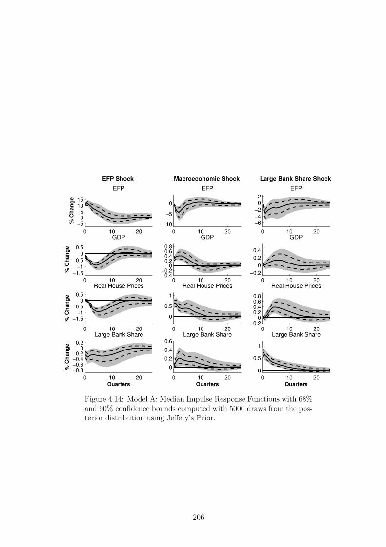
0 10 20

−505

1015

% C

han

ge

EFP Shock

EFP

0 10 20

−10

−5

0

Macroeconomic Shock

EFP

0 10 20

−6

−4

−2

02

Large Bank Share Shock

EFP

0 10 20

−1.5−1

−0.50

0.5

% C

han

ge

GDP

0 10 20−0.4−0.2

00.20.40.60.8

GDP

0 10 20

−0.2

0

0.2

0.4

GDP

0 10 20

−1.5−1

−0.50

0.5

% C

han

ge

Real House Prices

0 10 20

0

0.5

1

Real House Prices

0 10 20−0.2

00.20.40.60.8

Real House Prices

0 10 20

−0.8−0.6−0.4−0.2

00.2

% C

han

ge

Quarters

Large Bank Share

0 10 20

0

0.2

0.4

0.6

Quarters

Large Bank Share

0 10 20

0

0.5

1

Quarters

Large Bank Share

Figure 4.14: Model A: Median Impulse Response Functions with 68%and 90% confidence bounds computed with 5000 draws from the pos-terior distribution using Jeffery’s Prior.

206

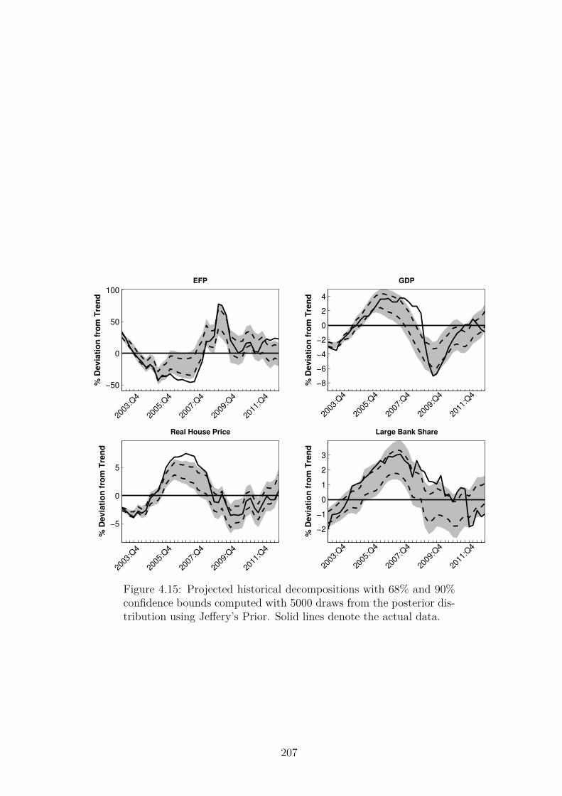
−50

0

50

100

2003

:Q4

2005

:Q4

2007

:Q4

2009

:Q4

2011

:Q4

% D

ev

iati

on

fro

m T

ren

d

EFP

−8

−6

−4

−2

0

2

4

2003

:Q4

2005

:Q4

2007

:Q4

2009

:Q4

2011

:Q4

% D

ev

iati

on

fro

m T

ren

d

GDP

−5

0

5

2003

:Q4

2005

:Q4

2007

:Q4

2009

:Q4

2011

:Q4

% D

ev

iati

on

fro

m T

ren

d

Real House Price

−2

−1

0

1

2

3

2003

:Q4

2005

:Q4

2007

:Q4

2009

:Q4

2011

:Q4

% D

ev

iati

on

fro

m T

ren

d

Large Bank Share

Figure 4.15: Projected historical decompositions with 68% and 90%confidence bounds computed with 5000 draws from the posterior dis-tribution using Jeffery’s Prior. Solid lines denote the actual data.

207

4.B Appendix: The Stationary, Non-Linear Model

In this section I provide the full set of equations which defines the dynamic equilibrium

model. All upper case variables are real and lower case variables are nominal - including

interest rates. In particular for any nominal interest rate rt, the real interest rate is given

via the Fisher equation, Rt = Et

rtπt+1

.

Household - 5

WHt

Ct=

ηLH

1−LNewt

(4.B.1)

WG,Ct

Ct=

ηL

1−LG,Ct

(4.B.2)

ηHtHt

=PHtCt

−βEt

(1− δH)PHt+1

Ct+1

(4.B.3)

1

rDt= Et Λt+1 (4.B.4)

Λt = βCt−1

πtCt(4.B.5)

208

Aggregate Goods Production - 7

Yt = ZGt (Kt−1)αG(

LGt)1−αG

(4.B.6)

LGt = (Lt)(1−αE)

(

LEt)αE

(4.B.7)

Wt = (1−αG)(1−αE)YtLt

(4.B.8)

WEt = (1−αG)αE

Yt

LEt(4.B.9)

rKt =αG

YtKt

+(1− δK)Qt

Qt−1(4.B.10)

CEt = (1−αNt )(1−Γt−1(ωt))RKt Kt−1 (4.B.11)

αNt =(1−Ft−1(ωt))P

Nt−1R

Dt−1N

(1−Γt−1(ωt))RKt Qt−1Kt−1(4.B.12)

Capital Producers - 1

It =Kt− (1− δK)Kt−1 (4.B.13)

Goods Production: Firm-level Debt Contract - 9

In this section I provide the equations which determine the debt contract. Moreover, I

provide a description of the individual entrepreneur’s problem which leads to the aggre-

gate entrepreneur’s consumption rule defined in equation (4.16). In particular, suppose

entrepreneuer j has preferences over consumption and housing given by a Cobb-Douglas

utility function,

Ut(j) = Ct(j)1−αN

t Nt(j)αN

t

209

with

αNt =(1−Ft−1(ωt))P

Nt−1R

Dt−1N

(1−Γt−1(ωt))RKt Qt−1Kt−1.

Since entrepreneuer j takes the aggregate default rate Ft−1(ωt) and the aggregate choice of

capital, Kt as given, this Walrasian demand bundles given these preferences has the well-

known property of constant expenditure shares on consumption and housing.

Ct(j) =(

1−αNt)(

1−Γt−1(ωjt ))

RKt Kjt−1Qt−1

Aggregating over this equation implies

Ct =

∞

0

(

1−αNt)(

1−Γt−1(ωjt ))

RKt Kjt−1Qt−1dj

=(

1−αNt)

(1−Γt−1(ωt))RKt Kt−1Qt−1

= (1−Γt−1(ωt))RKt Kt−1Qt−1 − (1−Ft−1(ωt))P

Nt−1R

Dt−1N.

The second equality follows from the ex-ante homogeneity among entrepreneurs implying

they all will choose the same default cut-off, ωjt , and the same level of capital expenditures,

Kjt .

210

Et

Γ′t(ωt+1)RKt+1QtKt

= λEt Et(

Γ′t(ωt+1)−µMG′

t(ωt+1))

RKt+1QtKt

(4.B.14)

Et

[1−Γt(ωt+1)]RKt+1

= λEt Et

REt −Γt(ωt+1)RKt+1

(4.B.15)

+λEt Et

µMGt(ωt+1)RKt+1

REt(

QtKt−PNt N −WEt

)

= Et

(

Γt(ωt+1)−µMGt(ωt+1))

RKt+1QtKt

(4.B.16)

Bt =QtKt−PNt N −WEt (4.B.17)

zt+1 =ln(ωt+1)+ .5(σωt )2

σωt(4.B.18)

Gt(ωt+1) = ΦN (zt+1 −σωt ) (4.B.19)

Γt(ωt+1) = ΦN (zt+1 −σωt )+ ωt+1

(

1−ΦN (zt+1))

(4.B.20)

G′t(ωt+1) =

(

1

σωt√

2π

)

e−z2t+12 (4.B.21)

Γ′t(ωt+1) = 1−ΦN (zt+1) (4.B.22)

Housing Production: Aggregate Behavior - 2

HNewt = ZHt (LHt )(1−αH) (4.B.23)

WHt = PHt (1−αH)

HNewt

LHt(4.B.24)

211

Productive Bank - 10

(1−ψtFt(ωt+1))BKPt

=NPt Et

ZRPHt+1 − (1−Ft(ωt+1))PNt RDt

PNt

(4.B.25)

Et

Λt+1rE,Pt

= Et

Λt+1rDt

(4.B.26)

Et

Λt+1rE,Pt

=

(

θB −1

θB

)

Et Λt+1 (1−Ft(ωt+1))rB,Pt (4.B.27)

+Et

Λt+1πt+1(1−µM )Φt(ωt+1)

Bt

BPt =

rB,Pt

rBt

−θB

Bt (4.B.28)

BPt =DP

t +BKP

t−1

πt−PNt N

Pt (4.B.29)

ΠPt = (1−Ft−1(ωt))

rB,Pt−1

πtBPt−1

+(1−µM )BPt−1

Bt−1Φt(ωt+1)

+(1−Ft−1(ωt))RDt−1P

Nt−1N

Pt−1 (4.B.30)

+Ft−1(ωt)PHt Z

RNPt−1 −PNt N

Pt

−RDt−1DPt−1 +DP

t −BPt

DIV Pt = ΠP

t (4.B.31)

TRANSPt = Ft−1(ωt)ψt−1BKP

t−1

πt(4.B.32)

INV Pt = TB,P −TRANSPt (4.B.33)

BKPt = INV P

t +(1− δBK,P )BKP

t−1

πt(4.B.34)

212

Unproductive Bank - 10

PNt =1

RDtEt

ZRPHt+1 −χR,UµR,UNU(χR,U−1)

t

(4.B.35)

Et

Λt+1rE,Ut

= Et

Λt+1rDt +χB,U

(4.B.36)

Et

Λt+1rE,Ut

=

(

θB −1

θB

)

Et Λt+1 (1−Ft(ωt+1))rB,Ut (4.B.37)

+Et

Λt+1πt+1(1−µM )Φt(ωt+1)

Bt

BUt =

rB,Ut

rBt

−θB

Bt (4.B.38)

BUt =DU

t +BKU

t−1

πt−PNt N

Pt (4.B.39)

ΠUt = (1−Ft−1(ωt))

rB,Ut−1

πtBUt−1

+(1−µM )BUt−1

Bt−1Φt(ωt+1)

+(1−Ft−1(ωt))RDt−1P

Nt−1N

Ut−1 (4.B.40)

+Ft−1(ωt)

[

PHt ZRNU

t−1 −µR,U(

NUt−1

)χR,U]

−PNt NUt −RDt−1D

Ut−1 +DU

t −BUt (1+χB,U )

DIV Ut = ΠU

t (4.B.41)

TRANSUt = Ft−1(ωt)ψt−1BKU

t−1

πt(4.B.42)

INV Ut = TB,U −TRANSUt (4.B.43)

BKUt = INV U

t +(1− δBK,U )BKU

t−1

πt(4.B.44)

213

Aggregate Bank - 10

rEt =[

ν(

rE,Ut

)1−θB +(1−ν)

(

rE,Pt

)1−θB

] 11−θB (4.B.45)

rEt =

(

θBθB −1

)

rEt −(

1

θB −1

)

(1−µM )Et

πt+1ΦH.B.t+1

Bt(4.B.46)

REt =rEtπt+1

(4.B.47)

RDt =rDtπt+1

(4.B.48)

rBt =[

ν(

rB,Ut

)1−θB +(1−ν)

(

rB,Pt

)1−θB

] 11−θB (4.B.49)

Dt = νDUt +(1−ν)DP

t (4.B.50)

DIVt = νDIV Ut +(1−ν)DIV P

t (4.B.51)

TRANSt = νTRANSUt +(1−ν)TRANSPt (4.B.52)

INVt = νINV Ut +(1−ν)INV P

t (4.B.53)

Φt−1(ωt) =Gt−1(ωt)RKt Qt−1Kt−1 (4.B.54)

Market Clearing - 4

Ht =HNewt +Ft−1(ωt)Z

RN +(1− δH)Ht−1 (4.B.55)

N = νNPt +(1−ν)NU

t (4.B.56)

Yt = Ct+CEt + It+ IBKt +µMΦt−1(ωt)+νFt−1(ωt)µR,U

(

NUt−1

)χR,U

+νχB,UBUt

(4.B.57)

GDPt = Ct+ It+PHt HINVt (4.B.58)

214

Monetary Policy - 2

ψt = ψ (4.B.59)

rDtrD

=(πtπ

)φπ

(4.B.60)

Exogenous Shocks - 5

ln(

ηHt)

=(

1−ρηH

)

ηH +ρηH ln(

ηHt−1

)

+ εηH

t (4.B.61)

ln(

ZGt)

= (1−ρZG)ZG+ρZGln(

ZGt−1

)

+ εZG

t (4.B.62)

ln(σωt ) = (1−ρσω)σω +ρσω ln(

σωt−1

)

+ εσω

t (4.B.63)

ln(

ZHt)

= (1−ρZH )ZH +ρZH ln(

ZHt−1

)

+ εZH

t (4.B.64)

ln(

ψN,Pt

)

=(

1−ρψN,P

)

ψN,P +ρψN,P ln(

ψN,Pt−1

)

+ εψN,P

t (4.B.65)

215

Chapter 5

The Foreclosure Accelerator versus

the Financial Accelerator: Housing

and Borrower’s Net Worth

5.1 Introduction

Newspaper articles, documentaries and general discussions about the 2008 financial crisis

center largely on the housing boom and bust now synonymous with the Great Recession.

However, much of the recent business cycle literature which has focused on integrating finan-

cial factors into general equilibrium models don’t feature housing markets (Christiano et al.,

2013; Justiniano et al., 2011). Figure (5.1) highlights the connection between the timing of

the fall in home prices, drop in output and pre-recession trough of finance premiums.

The disconnect between the general narrative regarding the role of housing in the worst

postwar recession and the analysis of business cycles is bridged in this paper. In order to

capture the above relationships, I develop a novel financial mechanism whereby firms rely on

housing secured debt instruments to finance their investment projects. When home prices

fall, the amount of secured debt firms can issue based upon a fixed amount of collateral

216

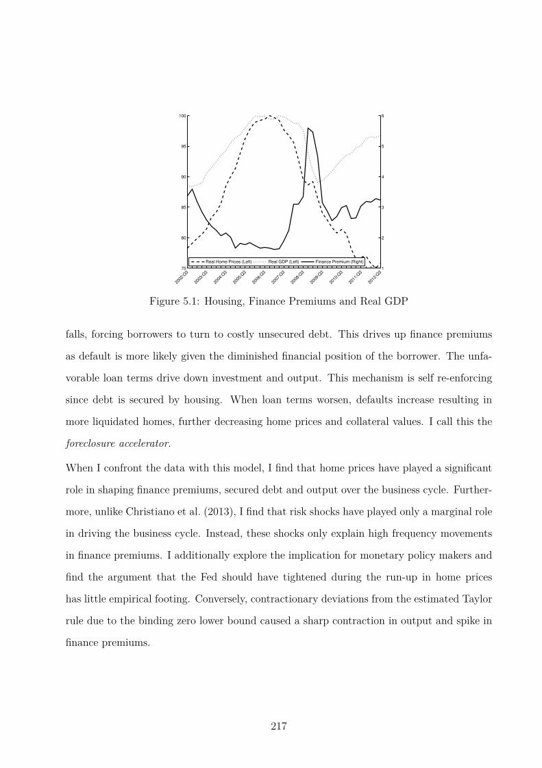
75

80

85

90

95

100

2002

:Q3

2003

:Q3

2004

:Q3

2005

:Q3

2006

:Q3

2007

:Q3

2008

:Q3

2009

:Q3

2010

:Q3

2011

:Q3

2012

:Q3

1

2

3

4

5

6

Real Home Prices (Left) Real GDP (Left) Finance Premium (Right)

Figure 5.1: Housing, Finance Premiums and Real GDP

falls, forcing borrowers to turn to costly unsecured debt. This drives up finance premiums

as default is more likely given the diminished financial position of the borrower. The unfa-

vorable loan terms drive down investment and output. This mechanism is self re-enforcing

since debt is secured by housing. When loan terms worsen, defaults increase resulting in

more liquidated homes, further decreasing home prices and collateral values. I call this the

foreclosure accelerator.

When I confront the data with this model, I find that home prices have played a significant

role in shaping finance premiums, secured debt and output over the business cycle. Further-

more, unlike Christiano et al. (2013), I find that risk shocks have played only a marginal role

in driving the business cycle. Instead, these shocks only explain high frequency movements

in finance premiums. I additionally explore the implication for monetary policy makers and

find the argument that the Fed should have tightened during the run-up in home prices

has little empirical footing. Conversely, contractionary deviations from the estimated Taylor

rule due to the binding zero lower bound caused a sharp contraction in output and spike in

finance premiums.

217

5.2 A DSGE Model with Integrated Housing

and Financial Markets

Here I take a medium-sized DSGE model and compliment it with a financial mechanism

which integrates housing and financial markets. The basic model, features sticky prices,

sticky wages, costly capital utilization, investment adjustment costs and habit-formation in

consumption. These factors significantly improve the model’s fit when it is confronted with

the data (See for e.g. Christiano et al. (2005); Smets & Wouters (2007)).

5.2.1 Model Description

The model consists of a continuum of infinitely lived households, a continuum of short-lived

entrepreneurs who produce the wholesale good using capital. New capital is produced by

perfectly competitive firms who use inputs from the perfectly competitive investment goods

producing sector. The introduction of these agents allows for time variation in the price of

investment goods and the price of capital. The financial sector is comprised by a continuum

of competitive banks which finances investment for goods producers. Lastly a central bank

is modeled. In this section I will describe the behavior of each agent in turn. I follow the

convention throughout the model that lower case variables are stationary and upper-case

variables are non-stationary.

5.2.1.1 Household

There are a continuum of households indexed by i ∈ [0,1] where each household i supplies

a differentiated labor. I assume as in Erceg et al. (2000) that household’s have access to a

complete state-contingent securities market so that households are homogeneous with respect

to consumption and asset holdings, but possibly heterogeneous with respect to their labor

income. This is reflected in my notation as I will index each household type i’s wage rate

and labor hours supplied, but not other household level variables.

The household earns labor income by renting labor to goods producers lt(i) and home builders

218

lht (i). Since household i supplies a differentiated type of labor they have some degree of

market power and therefore face the downward sloping demand for their labor variety:

lt(i) =

(

Wt(i)

Wt

)−θl

lt lht (i) =

(

W ht (i)

W ht

)−θl

lht (5.1)

In order to introduce sticky nominal wages I assume that households must pay an adjustment

cost similar to Rotemberg (1982). The specification of adjustment costs allows for the partial

indexation of wages to lagged wage inflation, πWt−1 and πW,ht−1 , and the central bank’s inflation

target, πt.

Households earn non-labor income from their ownership stake in retail firms, Ptst, and

principal plus interest payments Pt−1dt−1rDt−1 on last periods deposits. This income can be

saved in the form of bank deposits Ptdt or spent on consumption Ptct and housing P ht ht.

Also, any non-depreciated housing stock, (1− δ)ht−1, can be resold at the market price P ht .

The resulting budget constraint in any period t= 0,1,2, ... is given by:

Ptct+Ptdt+φW2

Wt(i)

Wt−1(i)πWϕlt−1 π

1−ϕlt

−1

2

Ptlt+φW2

W ht (i)

W ht−1(i)πW,hϕl

t−1 π1−ϕlt

−1

2

Ptlht

=Wt(i)lt(i)+W ht (i)lht (i)+Pt−1dt−1r

dt−1 −P ht

[

ht−(

1− δh)

ht−1

]

+Ptst.

The household maximizes their lifetime expected utility by choosing sequences for the vari-

ables

ct,ht,dt, lt(i), lht (i),Wt(i),W

ht (i)

∞

t=0while satisfying the flow budget constraint along

with the demands for their variety of labor. The household’s lifetime expected utility is

specified by:

U(i) =∞∑

t=0

βtE0

ηct

[

ln(ct−ct−1)+ηht ln(ht)−ηl,tlt(i)

1+νl

1+νl−ηhl,t

lht (i)1+νl

1+νl

]

,

ηct , ηht , ηl,t and ηhl,t represent shifts in the preferences over consumption goods, housing and

leisure. I specify these as exogenous processes, each of which follows a first order auto-

219

regressive process:

ln(ηct ) = ρηcln(ηct−1)+ εηc

t εηc

t ∼ N (0,σηc) , (5.2)

ln(ηht ) = (1−ρηh)ln(ηh)+ρηhln(ηht−1)+ εηh

t εηh

t ∼ N(

0,σηh

)

, (5.3)

ln(ηl,t) = (1−ρηl)ln(ηl)+ρηl

ln(ηl,t−1)+ εηlt εηl

t ∼ N (0,σηl) , (5.4)

ln(ηhl,t) = (1−ρηhl)ln(ηhl )+ρηh

lln(ηhl,t−1)+ εηl

t . (5.5)

Although I follow Iacoviello (2005) and Iacoviello & Neri (2010) by modeling a housing

market, I do not include household home equity borrowing constraints. I focus more so

on real-estate secured assets as collateral for investment and the interaction of house prices

and these assets. That being said, in general equilibrium changes in home prices can impact

consumption via traditional income and substitution effects, but not through the home equity

channel highlighted by Iacoviello (2005).

λt = Et

ηctct−ct−1

−βηct+1

ct+1 −ct

(5.6)

λtpht =

ηctηht

ht+β(1− δh)Et

λt+1pht+1

(5.7)

λt = βEt

λt+1rdt

πt+1

(5.8)

(1− θl)wt+ηl,tlt(i)

νl

λtθl = φW

πWt (i)

πWϕlt−1 π

1−ϕlt

−1

πWt (i)

πWϕlt−1 π

1−ϕlt

Wt

Wt(i)

−βφWEt

λt+1lt+1

λtlt

πWt+1(i)

πWϕlt π1−ϕl

t+1

−1

πWt+1(i)

πWϕlt π1−ϕl

t+1

Wt

Wt(i)

(5.9)

(1− θl)wht +

ηhl,tlht (i)νl

λtθl = φW

πW,ht (i)

πW,hϕlt−1 π1−ϕl

t

−1

πW,ht (i)

πW,hϕlt−1 π1−ϕl

t

W ht

W ht (i)

−βφhWEt

λt+1lt+1

λtlt

πW,ht+1 (i)

πW,hϕlt π1−ϕl

t+1

−1

πW,ht+1 (i)

πW,hϕlt π1−ϕl

t+1

W ht

W ht (i)

(5.10)

220

5.2.1.2 The Financial Sector

I assume a continuum of banks populate the financial sector. These banks, indexed by z,

make secured and unsecured loans to entrepreneurs who produce the consumption good.

These loans are funded entirely by deposits raised from the household. However, households

can not loan directly to entrepreneurs because they don’t have access to the monitoring and

liquidation technologies. Banks on the other hand are assumed to have access to technologies

which allow them to (1) monitor loan projects in order to verify default on unsecured loans

and (2) repossess and liquidate collateral posted for secured loans.

Since every bank z produces homogeneous outputs, no single bank has any degree of market

power. Thus, banks take as given the interest rate paid on deposits along with the interest

rate charged on secured and unsecured loans. Furthermore, I assume each bank can perfectly

diversify any idiosyncratic risk and therefore depositors can be guaranteed the same rate of

return across all banks. More specifically, borrowers who default on loans made in period

t−1, which occurs with probability Ft−1(ωt), have their assets seized by a collections agency

who distributes the proceeds, Υt−1(ωt), to banks in proportion to their loan market share

bzt−1/bt−1. Banks still bear the monitoring costs of confirming repayment was not possible

and therefore net only a fraction 1−µ of these proceeds.

Meanwhile, borrowers who default on their secured loan, which also occurs with probability

Ft−1(ωt), have their collateral repossessed by the bank and liquidated in the housing market.

Banks have access to technology which enables them to transform repossessed collateral into

housing at rate zr while bearing the time-varying real marginal liquidation costs of χrt :

ln(χrt ) = (1−ρχr)χrρχr ln(χrt−1)+ εχr

t εχr

t ∼ N (0,σχr) . (5.11)

Movements in χrt provide a proxy for financial innovation or differences in collateral from its

fundamental value that may arise in times of market illiquidity.

221

These receipts and outlays are summarized in bank z’s period t profit function below:

Πzt = (1−Ft−1(ωt))r

bt−1Pt−1b

zt−1 +(1−µ)Υt−1(ωt)

bzt−1

bt−1

+(1−Ft−1(ωt))Pnt−1n

zt−1r

dt−1 +Ft−1(ωt)

[

P ht zrnzt−1 −Ptχ

rt−1n

zt−1

]

−Pt−1dzt−1r

dt−1 +Ptd

zt −Pnt n

zt −Ptb

zt .

Bank z seeks to maximize the discounted present value of their profits subject to the balance

sheet constraint which stipulates that assets equal liabilities at all times. More formally, the

bank solves:

maxbz

t ,nzt ,d

zt ∞

t=0

∞∑

t=0

E0

M0|tΠzt

Pt

subject to Ptbzt +Pnt n

zt = Ptd

zt ,

where M0|t = βt λtλ0

is the stochastic discount factor derived from the household’s optimization

problem. The first order conditions from the bank’s problem will be useful when describing

the entrepreneurs in the following section. Therefore, they are provided below.

Et

Mt|t+1rdtπt+1

bt

= Et

Mt|t+1

(

(1−Ft(ωt+1))rbtπt+1

bt+(1−µ)Υt(ωt+1)

Pt+1

)

(5.12)

Et

Mt|t+1rdtπt+1

pnt

= Et

Mt|t+1

(

pHt+1zr −χrt

)

(5.13)

5.2.1.3 Wholesale Goods Production

The goods producing sector is comprised of a continuum of entrepreneurs. Entrepreneurs

have limited resources to finance capital required to produce the final good so they must

borrow from banks. A financial friction arises whereby entrepreneurs borrow funds from

banks this period to purchase capital used in production next period. Their output next

period is subject to idiosyncratic productivity disturbances only observable by banks after

paying a monitoring cost.

222

Entrepreneur’s Debt Contract: Housing Secured Debt

Entrepreneurs are risk-neutral agents who supply wholesale goods to retailers using capital

and labor. Here I use the large-family metaphor and assume that each household type i has

a large number of entrepreneurs.1 These entrepreneurs are indexed by j ∈ R+, where the

index corresponds to their liquid assets, denoted ajt at the beginning of period t. In addition

to these liquid assets, each entrepreneur is endowed with 1 unit of labor supply in period t

and n units of an asset which can be transformed into housing only by entrepreneurs and

banks in period t+1. However, capital must be purchased in period t to be useful in period

t+ 1. Denote the quantity of capital purchased in period t by entrepreneur j by kjt and

denote the period t nominal price of capital by Qt. To purchase this capital the entrepreneur

will receive financing from the banking sector. More specifically, the entrepreneur use their

liquid assets (which includes their wages earned in period t) and pledges their t+1 housing

security endowment n as collateral for a secured loan in the amount Pnt n. The remaining

portion of the capital purchase is financed with an unsecured loan in the amount Ptbjt . More

concretely,

Qtkjt = Pnt n+Ptb

jt +Pta

jt (5.14)

is entrepreneur j’s budget constraint.

Without default, distinguishing between secured and unsecured loans is trivial. However, in

period t+ 1, entrepreneurs are subjected to an idiosyncratic productivity shock ωjt+1 which

is i.i.d. across entrepreneurs and time. I assume throughout the analysis in this paper,

ωjt+1 ∼ lnN(

−(σωt )2

2 ,σωt

)

with CDF at time t denoted by Ft (ωt+1). The choice of parameters

implies E

ωjt+1

= 1 so that in the aggregate this idiosyncratic shock has no direct impact

on production, but the existence of uncertainty at the firm level impacts aggregate output

through financial imperfections (BGG).

1This assumption, as in Christiano et al. (2013), makes only 1 minor change to the equilibrium equationswhen compared to the set-up in Bernanke et al. (1999) who don’t assume the entrepreneurs live with thehousehold.

223

To capture exogenous changes in the cross-sectional dispersion of idiosyncratic productivity

shocks I allow σωt to vary over time. I posit the simple auto-regressive process,

ln(σωt ) = (1−ρσω)ln(σω)+ρσω ln(σωt−1)+ εσω

t εσω

t ∼ N (0,σσω) (5.15)

for this demand-side risk shock. Christiano et al. (2013) show that such shocks have played

a significant role in shaping the U.S. business cycle.

Since projects are financed before the idiosyncratic productivity shock can be observed by

either the entrepreneur or the bank, entrepreneurs who receive a low productivity value

will default upon their loan. Denote the gross interest rate on unsecured loans paid by

entrepreneur j by rb,jt and denote the gross return on capital common to all entrepreneurs

by rkt+1. Then for any entrepreneur j, we can define the cut-off value of ωjt+1 by the equation

ωjt+1rkt+1k

jtQt = Ptb

jtrb,jt . (5.16)

This equation defines the minimum level of productivity needed to pay back the unsecured

loan. For entrepreneur j, the loan will be repaid if ωjt+1 ≥ ωjt+1 and will otherwise be

defaulted upon. However, the bank can not observe the level of productivity without paying

an auditing cost in proportion µ ∈ (0,1) to the entrepreneur’s revenue.2 Banks who do

not pay for auditing never find out if the entrepreneur actually received a low productivity

draw or if they simply chose to renege on their loan. Given this arrangement, the optimal

debt-contract from the borrowers perspective dictates that banks will audit only defaulting

entrepreneurs and only entrepreneurs who receive a bad-draw will default on their loans.

Although the contract is optimal from the borrower’s perspective, the entrepreneur must

ensure the bank’s profit maximization condition from (5.12) is satisfied. More strictly, the

debt-contract must be individually rational from the bank’s perspective in every state of

2This follows from Townsend (1979), but has been popularized in this context by Carlstrom & Fuerst(1997) and BGG.

224

nature since the banks are owned by risk-averse households. This implies the risk-neutral

entrepreneurs bear all the aggregate risk, and the bank’s optimality condition (5.12) holds

both in and out of expectation:

rdt bjt

︸ ︷︷ ︸

Funding Cost

=(

1−Ft(ωjt+1)

)

rb,jt bjt︸ ︷︷ ︸

Non-Defaulting Payoff

+(1−µ)

ˆ ωjt+1

0ωjt+1dFt(ω

jt+1)rkt+1k

jt qt

︸ ︷︷ ︸

Defaulting Payoff

(5.17)

where

υt(ωt+1) ≡ Υt(ωt+1)

Pt+1=

ˆ ωjt+1

0ωjt+1dFt(ω

jt+1)

rkt+1

πt+1kjt qt. (5.18)

We can simplify this expression (and the resulting entrepreneur’s optimization problem) by

defining the following terms. First let Gt(ωjt+1) be defined as the expected productivity value

for defaulting entrepreneurs.

Gt(ωjt+1) =

ˆ ωjt+1

0ωjt+1dFt(ω

jt+1) (5.19)

Also let Γt(ωjt+1) be defined as the expected share of entrepreneurial profits going to the

bank gross of auditing costs.

Γt(ωjt+1) =

(

1−Ft(ωjt+1)

)

ωjt+1 +Gt(ωjt+1) (5.20)

Now I can combine (5.17) with (5.14), (5.16), (5.19) and (5.20) to rewrite the bank’s indi-

vidual rationality constraint as follows:

rdt(

qtkjt −pnt n−ajt

)

=(

Γt(ωjt+1)−µGt(ω

jt+1)

)

rkt+1kjt qt. (5.21)

We can now formally state the problem faced by entrepreneur j. To keep the debt-contract

tractable, I assume the entrepreneur is instructed by the household to maximize their period

t+ 1 income (as a random fraction, 1 − γt, is transferred to households) and in exchange

225

entrepreneurs receive consumption insurance from household’s. Entrepreneurs who succeed,

are contractually obligated to pay-back their secured loan, prior to transferring funds to

homeowners. Since homeowners own the banks, they yield to the seniority of the debt

structure.

Entrepreneur j therefore seeks to maximize the gross expected income (of which the fraction

(1−γt) is transferred to their household), subject to (5.21):

maxkj

t ,ωjt+1

Et

(

1−Γt(ωjt+1)

)

rkt+1kjt qt

subject to rdt(

qtkjt −pnt n−ajt

)

=(

Γt(ωjt+1)−µGt(ω

jt+1)

)

rkt+1kjt qt

Where I use (5.16) and (5.20) to write Et

´∞ωj

t+1ωjt+1dF (ωjt+1)rkt+1k

jt qt− (1−Ft(ω

jt+1))rb,jt bjt

= Et

(1−Γt(ωjt+1))rkt+1k

jt qt

. The solution to this optimization problem pins down the cut-

off value ωjt+1 and the entrepreneur’s demand for capital kjt .

Et

(

1−Γt(ωjt+1)

)

rkt+1 − Γ′t(ω

jt+1)

Γ′t(ω

jt+1)−µG′

t(ωjt+1)

[

rdt −(

Γt(ωjt+1)−µGt(ω

jt+1)

)

rkt+1

]

= 0

(5.22)

The problem is identical in nature to the problem entrepreneurs face in BGG who show the

optimal debt contract has the property that the default rate, Ft(ωjt+1), and external finance

premium, rkt /rdt−1, move inversely with net-worth. In this model, the net-worth component is

replaced with the collateral value and wage earnings, pnt n+wEt , implying that ∂ωjt+1/∂pnt < 0

- finance premiums and default rates will move in the opposite direction of collateral prices.

From (5.13), this implies finance premiums will move in the opposite direction of home prices.

Aggregate Wholesale Goods Production

The previous section describes the firm-level behavior in the wholesale goods producing sec-

tor, specifically it describes the debt-contracting problem faced by each producer. In this

section, I describes the industry wide behavior. Since each entrepreneur (in the second period

of their life) has access to the homogeneous production technology, yjt = ωjt(

kjt−1

)α(

l′jt)1−α

,

226

which can be aggregated over due to constant returns to scale. The aggregate goods pro-

duction technology in any given period t is specified as

yt = zt(

kt−1

)α(

l′t)1−α

(5.23)

where zt is an exogenous technology process which affects all entrepreneurs equally. I assume

this technology follows a first-order autoregressive process.

ln(zt) = ρzln(zt−1)+ εzt εzt ∼ N (0,σz) (5.24)

Wholesale producers use this technology to produce the wholesale good which is purchased

by retailers. This wholesale goods market is perfectly competitive and therefore the wholesale

price, PWt , is taken as given. We can now consider the determination of factor demands for

capital and labor.

The labor aggregate in the production function is a composite of labor supplied by the

household, lt ,and labor supplied by this periods young entrepreneurs, lEt ,

l′t =(

lEt)αE(

lt)1−αE

, (5.25)

where αE captures the share of goods producing income received by entrepreneurs. This

implies the wage paid to the household’s labor and the wage paid to entrepreneurial labor

are given by:

Wt = PWt (1−α)(1−αEt )ytlt

(5.26)

WEt = PW (1−α)αEt

yt

lEt. (5.27)

227

Similarly, the marginal product of capital is given by:

mpkt = αytkt−1

(5.28)

The gross nominal return on holding a unit of capital from period t−1 to period t is defined

by

rkt =utmp

ktP

Wt −a(ut)Pt+(1− δk)Qt

Qt−1, (5.29)

where ut is the utilization rate chosen by the producers and a(ut) are the real resources spent

to support this utilization rate:

a(ut) =mpk

χa

[

eχa(ut−1) −1

]

. (5.30)

The only way the utilization rate impacts entrepreneurs is through (5.29). Therefore, en-

trepreneurs solve the problem:

maxut

rkt (5.31)

Hence, from this point on, ut represents the optimal utilization rate and satisfies the first

order condition:

mpkt pWt =mpkpW eχ

a(ut−1), (5.32)

where the specification of a(ut) ensures that u= 1 so steady state utilization costs are zero.

Notice that in (5.32), the first order condition for choosing ut to maximize rkt , and in (5.22),

the optimal choice of ωj are both independent of each entrepreneur’s liquid assets. Hence,

the distribution of the liquid assets across entrepreneurs is not needed to determine aggre-

gate capital stock and loans.3 Hence, the aggregate income of entrepreneurs in period t is

(1−Γt−1(ωt))rk

tπt+1

kt−1qt−1. Entrepreneurs have the ability to transform their endowment n

- into non-tradable housing. Recall however, this endowment was leveraged last period to

3See equations 2.15 and 2.16 in Christiano et al. (2013) for more details on the aggregation across en-trepreneurs.

228

secure a loan in the amount pnt−1n. Hence, entrepreneurs who are able, choose to payback

the secured loan with interest pnt−1nrdt−1 and then convert n into housing services one for

one. If they don’t payback the secured loan then they default on this contract and the bank

takes possession of the collateral n.

I assume in the aggregate, all the entrepreneurs who did not default on their unsecured

loan, payback their secured loan and divide the rest of their income between transfers to

households and liquid assets next period so that at evolves according to:

at = γ

[

(1−Γt−1(ωt))rktπtkt−1qt−1 − (1−Ft−1(ωt))p

nt−1n

rdt−1

πt

]

+wEt . (5.33)

A more elaborate specification would make the entrepreneur’s decision of whether to pay-back

their secured loan a strategic choice of the entrepreneur; whereas, this specification implies

the only source of default on secured loan is due to insufficient income. An appealing aspect

of this description is the existence of a single default rate in the economy.4 Moreover, this

specification captures the essence of securing debt with mortgage backed securities. When

the default rate of mortgages rise, financial firms (investment banks for example) who rely

on these payments to fund their debt (which further fund MBS purchases and nonfinancial

firms projects) are more likely to default. These risk cause secured loan markets to dry-

up. Interpreting the entrepreneur as an investment bank who funds non-financial firms in a

market without imperfections yields such an interpretation.

5.2.1.4 Retail Goods Producers

Retailers are monopolistically competitive firms who purchase the generic wholesale good at

price PWt and transform it into a unique variety. Due to the differentiated nature of each

firm’s, f ∈ [0,1], output they face a downward sloping demand for their variety of the final

4That is to say, the default rate on unsecured loans is the same as the default rate on secured loans. Ichoose this as a starting point although this assumption can be relaxed.

229

good:

yt(f) =

(

Pt(f)

Pt

)−θt

yt (5.34)

where variations in θt appear as “Cost Push,” or non-technology supply shocks in the log-

linearized New-Keynesian Phillips Curve that emerges from the retailer’s first order condi-

tion. I assume as in Smets & Wouters (2007):

ln(θt) = (1−ρθ)θ+ρθln(θt−1)+ εθt εθt ∼ N (0,σθ) . (5.35)

Given the market power of retail firms, each firm f would like to sell their variety for a rent

maximizing mark-up over marginal cost. However, to introduce nominal price rigidities, I

assume firms also bear a convex cost of adjusting their price relative to the rate of inflation

as in Rotemberg (1982). More specifically, retailers seek to maximize the discounted sum of

their real dividend stream:

maxPt(f)∞

t=0

∞∑

t=0

E0

M0|t

Pt(f)

Ptyt(f)− PWt

Pt− φ

2

Pt(f)

Pt−1(f)πϕt−1π1−ϕt

−1

2

yt

subject to (5.34).

(5.36)

In a symmetric equilibrium where Pt(f) = Pt∀f , the resulting first order condition defines

the typical forward-looking aggregate supply relationship relating inflation to real marginal

cost. In other words, the New-Keynesian Phillips Curve emerges from the firm’s problem.

θtpWt

(

Pt(f)

Pt

)−θt−1

− (θt−1)

(

Pt(f)

Pt

)−θt

= φ

πt(f)

πϕt−1π1−ϕt

−1

πt(f)

πϕt−1π1−ϕt

PtPt(f)

(5.37)

−φEt

yt+1Mt,t+1

ytMt,t

[

πt+1(f)

πϕt π1−ϕt

−1

]

πt+1(f)

πϕt π1−ϕt

PtPt(f)

5.2.1.5 New Housing Production

I assume new housing is produced in a purely competitive market and free from financial

frictions. In particular, housing producers combine labor lht with housing specific technology,

230

zht in the production technology,

hnewt = zht (lht )1−αh

(5.38)

where

ln(zht ) = ρzhln(zht−1)+ εzh

t εzh

t ∼ N (0,σzh) . (5.39)

I model housing specific technology independent of technology in the goods producing sec-

tor since much of the economic growth over the last two decades has been IT-driven and

housing production is a non IT-intensive industry. Moreover, this specification allows for

the technology process in the goods producing sector, zt, to potentially play a significant

role in determining output without implying a counterfactual negative correlation between

home prices and GDP (see for example Davis & Heathcote (2005)). The resulting demand

for labor from the housing sector takes the form:

W ht = P ht (1−αh)

hnewt

lht. (5.40)

5.2.1.6 Investment Goods Production

Perfectly competitive firms purchase yit units of the final retail good at a price of Pt and use

the linear, time-varying technology:

it = zityit (5.41)

to transform these retails goods into investment goods, which they sell to capital goods

producers for a market determined price P it . The representative investment goods producing

firm solves the following problem:

maxyi

t

P it zityit −Pty

it, (5.42)

231

which pins down the relative price of investment as:

P itPt

=1

zit. (5.43)

The purpose of explicitly including this sector in the model is to examine the role investment-

specific technology play in shaping the business cycle. During the estimation the price of

investment goods relative to consumption goods, pit = P it /Pt is treated as an observable

variable which disciplines the estimation of the zit process:

ln(zit) = ρziln(zit−1)+ εzi

t εzi

t ∼ N (0,σzi) . (5.44)

5.2.1.7 Capital Goods Production

In period t, the capital goods producing firm purchases any non-depreciated capital from

period t− 1 at the market price Qt and produces new capital using the investment good

which is purchased at the price P it . The sum of these two components comprises the total

capital stock at the end of period t, which is sold to entrepreneurs at the price Qt. The rate at

which the capital goods producers can transform the investment good and old, undepreciated

capital into new capital is constrained by the technology:

kt =

(

it−S

(

it

zkt kt−1

)

zkt kt−1

)

+(1− δk)kt−1 (5.45)

where S(·) captures cost of adjusting the level of investment. This function has the properties

that S(δk) = S′(δk) = 0 and S′′(δk)> 0. In practice, these derivatives can be matched with

the function:

S

(

it

zkt kt−1

)

=χS

2

[

it

zkt kt−1− δk

]2

where χS > 0. (5.46)

In the financial accelerator model of Bernanke et al. (1999) and Christiano et al. (2013), this

function plays a critical role in the propagation of downturns by endogenously decreasing

the price of capital when investment falls. This drop in asset prices decreases th net worth

232

of entrepreneurs in these models which ultimately leads to further reductions in investment,

starting the cycle over. This is the celebrated financial accelerator mechanism.

Meanwhile the term zkt in (5.45) captures variations in the efficiency at which the investment

goods can be transformed into installed capital:

ln(zkt ) = ρzk ln(zkt−1)+ εzk

t εzk

t ∼ N (0,σzk) . (5.47)

In Justiniano et al. (2011), movements in zkt make the largest contribution to output, in-

vestment and labor dynamics at business cycle frequencies. However, the bulk of these

movements correspond to financial distress. Therefore it is perhaps not surprising that when

these shocks are included in the estimation of the enriched BGG/financial accelerator model

of Christiano et al. (2013), movements in σωt overtake movements in zkt as the most important

shocks at business cycle frequencies. The framework presented in this paper allows these

shocks to compete with housing demand disturbances in driving the business cycle. The

capital goods producer solves:

maxkt,it

Qtkt−Qt(1− δk)kt−1 −P it it subject to (5.45), (5.48)

which implies the following Tobin’s Q relationship:

Qt =P it

1−S′(

itzk

t kt

) . (5.49)

5.2.1.8 Central Bank

The central bank is charged with setting monetary policy. The monetary policy instrument

is the rate on 1-period deposits, rdt , which is assumed to follow a linear (in logs) feedback

233

rule of the type specified by Taylor (1993):

rdtrd

=

(

rdt−1

rd

)ρr(

πtπt

)ψπ(

ytyt−1

)ψy

ǫrt ǫrt,4 (5.50)

where,

ln(ǫrt ) = εrt εrt ∼ N (0,σr) (5.51)

ln(ǫr,4t ) = ρr,4 ln(ǫr,4t−1)+ εr,4t−4 εr,4t ∼ N (0,σr,4) . (5.52)

There are three senses in which this rule evolves stochastically. First, there is a typical

monetary policy shock, ǫrt which is completely unforecastable by agents. However, I also

allow for the possibility that agents learn the central bank is going to deviate from their

policy rule in the future through the exogenous term ǫr,4t . Although the solution method

employed to estimate the model parameters doesn’t allow for explicitly incorporating agents’

knowledge of the zero lower bound on nominal interest rates, these news shocks allow for

deviations which are not a surprise to agents.

A third sense in which the policy rule evolves stochastically arises from the central bank’s

inflation target, πt which evolves according to an AR(1) process:

ln(πt) = (1−ρπ)π+ρπln(πt−1)+ επt επt ∼ N (0,σπ) . (5.53)

This shock is introduced as a means of capturing the downward trend in inflation in the

early part of the sample. To this end, I set ρπ = 0.975 and σπ = 0.0001 (Christiano et al.,

2013).

5.2.1.9 Market Clearing

Sections 5.2.1.1 - 5.2.1.8 describe the optimal behavior of all agents in the economy. A

symmetric competitive equilibrium is defined as a sequence of quantities, prices and Lagrange

multipliers (shadow prices) which satisfy all optimality conditions, policy rules and market

234

clearing conditions. In particular, symmetry across households implies that:

lt(i) = lt (5.54)

Wt(i) =Wt (5.55)

lht (i) = lht (5.56)

W ht (i) =W h

t . (5.57)

Symmetry across banks implies:

bzt = bt (5.58)

dzt = dt (5.59)

nzt = nt. (5.60)

Symmetry across entrepreneurs implies:

bjt = bt (5.61)

kjt = kt. (5.62)

Similarly, symmetry across retailers implies:

Pt(f) = Pt (5.63)

yt(f) = yt. (5.64)

The market clearing condition in the collateralized loan market requires that at all times:

nt = n. (5.65)

235

Using this requirement, the housing market clearing condition can be expressed as:

ht = hnewt +Ft−1(ωt)zrn+(1− δh)ht−1. (5.66)

Using the collateralized loan market clearing again, the goods market clearing condition can

be expressed by the resource constraint:

yt = ct+pitit+Ft−1(ωt)χrn+µυt−1(ωt)+a(ut)+act, (5.67)

where act defines the real-resource cost of adjusting prices and wages:

act =φ

2

πt

πϕt−1π1−ϕt

−1

2

yt+φW2

πWt

πϕlt−1π

1−ϕlt

−1

2

lt+φW2

πW

h

t

πϕlt−1π

1−ϕlt

−1

2

lht . (5.68)

Since act is of second-order, in a linear approximation we have that act ≈ 0.

It is useful for the purpose of model inference to define gross domestic product in this multi-

sector model:

gdpt = ct+pitit+pht hnewt . (5.69)

5.3 Model Inference

In this section I describe the econometric strategy employed to estimate the model’s param-

eters. I discuss the data used in this analysis, the choice of priors with an emphasis on the

relative tightness of the prior specifications and finally the specification of news shocks and

examination of model fit.

5.3.1 Data

I use quarterly data on 11 variables spanning 1990:Q1 to 2013:Q4. 7 variables are standard

macroeconomic time-series including: consumption, non-residential investment, the relative

price of non-residential investment goods, the federal funds rate, inflation, the real wage

236

rate and hours worked. Since there are multiple sectors in the model, including the real

wage rate and hours worked in both sectors would require bringing in more variables to

the analysis, limiting the number of financial variables I could introduce without inducing

stochastic singularity. To avoid this issue I compute the aggregate real wage rate, wat , and

hours worked, lat , as a Tornquist-Thiel (or Divisia) index number:

ln

(

latlat−1

)

=1

2(sht + sht−1)ln

(

lhtlht−1

)

+1

2(st+ st−1)ln

(

ltlt−1

)

(5.1)

ln

(

watwat−1

)

=1

2(sht + sht−1)ln

(

whtwht−1

)

+1

2(st+ st−1)ln

(

wtwt−1

)

. (5.2)

where st = wtlt/(wtlt +wht lht ) is the share of income earned in the goods producing sector

and sht = 1−st is the share of income earned in the housing sector. For the data component,

I use BLS aggregate measures of hours worked and wages earned in the private sector.

The remaining 4 variables consist of housing and financial market variables. The 2 housing

market variables include residential fixed investment and real home prices, measured using

the S&P/Case-Shiller National Composite Home Price Index. The remaining 2 variables

are financial variables. As Christiano et al. (2013) show, including financial variables in the

estimation is critical to capturing the role credit frictions play in the business cycle. Most

critical of these variables is the external finance premium, rkt /rdt−1 − 1 = µυt−1(ωt)

bt−1which

is measured empirically as the difference between BAA-rated corporate bonds and the 10-

year U.S. government bond rate. Again, similar to Christiano et al. (2013) I inform my

estimation on the measure of credit using data on credit to non-financial firms from the

Flow of Funds dataset. In particular, bt+pnt n is measured as the (first log difference in) the

‘credit market instruments’ measure of total liabilities for nonfarm, nonfinancial corporate

and noncorporate business.

237

5.3.2 Parameters: Calibration and Prior Specification

The model has a total of 54 parameters. I will divide these parameters into 3 groups:

calibrated parameters, parameters with tight priors, parameters with loose priors. The logic

of the partition is as follows. Several pairs of parameters are likely to not be jointly identified

and therefore one of the pair must be calibrated prior to estimation. Also, several parameters

such as capital’s share in the production function and the depreciation rate of capital are

standard in macroeconomic models and therefore can be easily calibrated. Moreover, the

model variables are by construction in log-deviations from steady state and therefore are

mean zero. Hence, for the data to align with the construction of the model variables all data

is demeaned. That being said, the information contained in the first moment need not be

disposed. Instead, this information can be brought into the model by specifying the values

of parameters which determine the model’s steady state. This information thus plays a role

in the calibration and specification of priors.

5.3.2.1 Calibrated Parameters

It is well known the discount rate β and depreciation rates δh and δk are not jointly identified.

To avoid this potential pitfall, I use the consensus value of δk = 0.025. At the same time,

I set n to ensure the steady state return on capital is rk = 1.025. Moreover, I fix β so that

rd = π/β = 1.015 where π represents the mean of the central bank’s inflation target. These

two facts imply a steady-state difference between the risky loan rate and the policy rate

equals to 4.00% annually, the average spread between the BAA-corporate bond rate and the

federal funds rate, according to data obtained from the St. Louis Fed’s FRED database.

The housing depreciation parameter, δh is calibrated to 0.0123 which implies, along with

the other means of the prior distributions, that the steady state ratio of housing wealth to

annual GDP equals 1.4. In other words, δh = ph(hnew+F (ω)zrn)1.4×4×gdp . Following Christiano et al.

(2013) I fix the inflation target at π = 1.0051 so that inflation averages 2.4% per year. As

noted in the text, to capture the downward trend in inflation during the early part of the

238

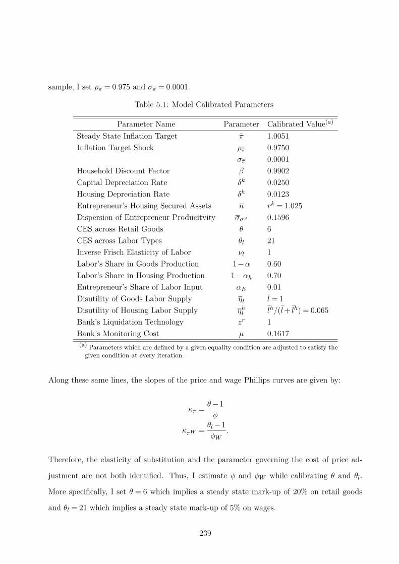
sample, I set ρπ = 0.975 and σπ = 0.0001.

Table 5.1: Model Calibrated Parameters

Parameter Name Parameter Calibrated Value(a)

Steady State Inflation Target π 1.0051

Inflation Target Shock ρπ 0.9750

σπ 0.0001

Household Discount Factor β 0.9902

Capital Depreciation Rate δk 0.0250

Housing Depreciation Rate δh 0.0123

Entrepreneur’s Housing Secured Assets n rk = 1.025

Dispersion of Entrepreneur Producitvity σσω 0.1596

CES across Retail Goods θ 6

CES across Labor Types θl 21

Inverse Frisch Elasticity of Labor νl 1

Labor’s Share in Goods Production 1−α 0.60

Labor’s Share in Housing Production 1−αh 0.70

Entrepreneur’s Share of Labor Input αE 0.01

Disutility of Goods Labor Supply ηl l = 1

Disutility of Housing Labor Supply ηhl lh/(l+ lh) = 0.065

Bank’s Liquidation Technology zr 1

Bank’s Monitoring Cost µ 0.1617

(a) Parameters which are defined by a given equality condition are adjusted to satisfy thegiven condition at every iteration.

Along these same lines, the slopes of the price and wage Phillips curves are given by:

κπ =θ−1

φ

κπW =θl−1

φW.

Therefore, the elasticity of substitution and the parameter governing the cost of price ad-

justment are not both identified. Thus, I estimate φ and φW while calibrating θ and θl.

More specifically, I set θ = 6 which implies a steady state mark-up of 20% on retail goods

and θl = 21 which implies a steady state mark-up of 5% on wages.

239

As for the production technologies, I set α= 0.4 which implies labor’s share of income in the

goods producing sector is 60%. Following Iacoviello & Neri (2010), I set αh = 0.3. Finally,

as in Bernanke et al. (1999), I set αE = 0.01. The household’s preferences over labor are

specified so that the curvature on the disutility of labor, νl = 1. There are no natural units

of hours worked in the model. Hence, I normalize the steady state hours worked in the goods

producing sector to 1 and use the empirical fact that the average share of hours worked in

construction relative to all sectors is lh/(lh + l) = 0.065. This value is found in U.S. data

produced by the BLS. I adjust ηl and ηhl so that the household’s preferences are consistent

with this steady state. As for the banking parameters, zr and χr are likely to be weakly

identified jointly. Therefore, I normalize zr = 1 and estimate χr.

5.3.2.2 Prior Specification

The remaining 38 parameters are estimated using Bayesian methods. Of these parameters, 24

govern of the persistence and standard deviation of the exogenous shock processes. Since the

central question of this paper is the relative importance of housing secured debt instruments

and therefore the importance of shocks which drive home prices and the business cycle,

I remain agnostic about the prior importance of all shocks. For all of these processes, I

specify a Beta prior on the auto-correlation terms with mean 0.8 and a standard deviation

of 0.1. For the standard deviation of the white noise shocks which drive the model, I take a

similar agnostic stand and specify and Inverse-Gamma prior with mean 0.001 and standard

deviation 0.01.

The 14 remaining parameters allow for considerably more information to be imparted into

the prior. Beginning with the costs of price and wage adjustment, there are wide ranging

estimates (see for example Keen & Wang (2007)). One obvious way to interpret the value is to

use the implied equivalence between the Calvo and Rotemberg approach to nominal rigidities.

In particular, the two approaches yield identical New-Keynesian Phillips Curves, when the

slope terms are calibrated so that: (1−ξ)(1−βξ)ξ = θ−1

φ . This equality implies that for a given

probability of prices remaining fixed ξ ∈ [0,1], the corresponding cost of price adjustment φ

240

lies in [0,∞). To keep the supports of the priors for φ and φW compact, I specify a Beta

prior for ξ and ξW and apply the above transformation to find the corresponding cost of

price and wage adjustment. The prior means are consistent with prices and wages remain

unchanged for on average 2 quarters and 4 quarters respectively.

The prior for the steady state fraction of liquid assets retained by entrepreneurs, γ, monitor-

ing costs µ, repossession cost χr and cross-sectional variance of productivity shocks across

entrepreneurs σω, are calibrated to match the following empirical facts (with all other pa-

rameters set to their prior mean): The average ratio of liquid assets to secured loans is equal

to 0.42, the average ratio of secured loans to all firm liabilities is 0.21, the average annual

business failure rate is 0.04 and residential investment’s share of GDP is 0.0541.5

The model is able to exactly match these facts and for this reason I calibrate µ= 0.1617 and

σω = 0.1596, which can be interpreted from the Bayesian perspective as specifying extremely

tight priors.6 For the remaining parameters, the implied values from this moments matching

exercise implies the following specifications of the prior distributions: γ is distributed as

a Beta with mean 0.9103 and standard deviation 0.10 and χr is distributed Log-Normally

with mean 0.3109 and standard deviation 0.10. Although many of these variables are used

as observables in the estimation, all of the data are demeaned. Hence, matching the model’s

steady state with these sample means does not contaminate the priors.

The remaining parameters do not determine any steady state outcomes. Therefore, I specify

rather loose priors for these parameters so that the econometrics specification has consider-

able flexibility to match the dynamics in the data. I specify the elasticity of the adjustment

cost function, χa, as a Log-Normal with mean 1.0 and standard deviation 1.0. Similarly,

the elasticity of the capital adjustment cost function χS , is specified as a Log-Normal with

mean 5.0 and standard deviation 5.0. Similarly, I set the prior for the price indexation, wage

5The housing preference shock’s mean ηh, is set so that pn = 1 in steady state. This normalization isnecessary since n and pn are not separately identifiable given this information.

6Calibrating these parameters, as opposed to estimating them, also leads to a considerably more efficientalgorithm to solve for the model’s steady state. This therefore speeds-up the estimation significantly.

241

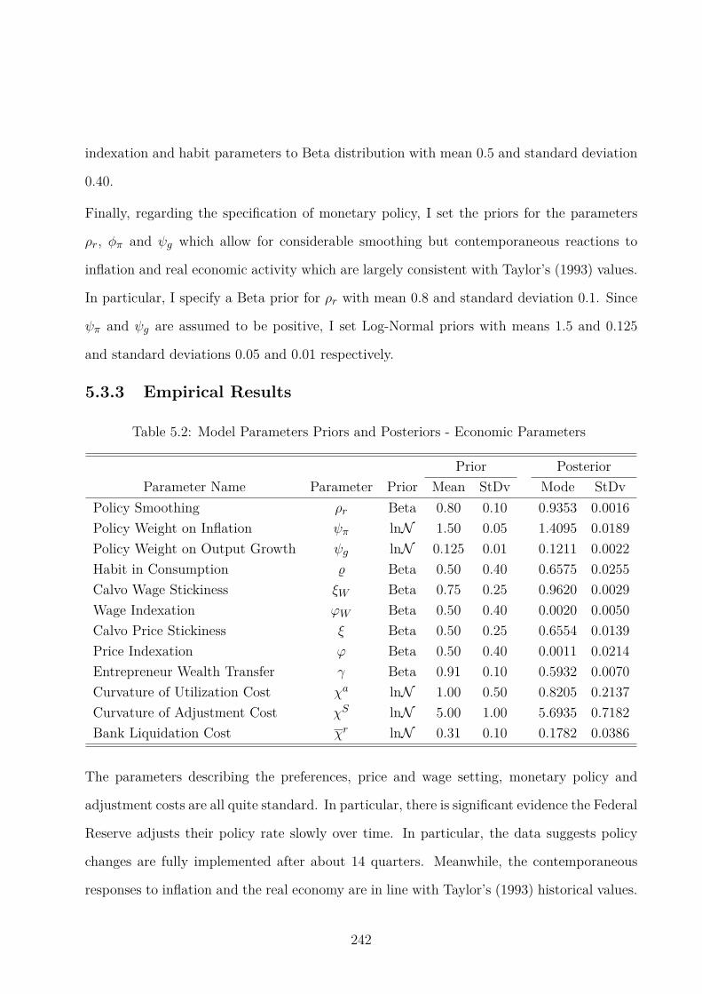
indexation and habit parameters to Beta distribution with mean 0.5 and standard deviation

0.40.

Finally, regarding the specification of monetary policy, I set the priors for the parameters

ρr, φπ and ψg which allow for considerable smoothing but contemporaneous reactions to

inflation and real economic activity which are largely consistent with Taylor’s (1993) values.

In particular, I specify a Beta prior for ρr with mean 0.8 and standard deviation 0.1. Since

ψπ and ψg are assumed to be positive, I set Log-Normal priors with means 1.5 and 0.125

and standard deviations 0.05 and 0.01 respectively.

5.3.3 Empirical Results

Table 5.2: Model Parameters Priors and Posteriors - Economic Parameters

Prior Posterior

Parameter Name Parameter Prior Mean StDv Mode StDv

Policy Smoothing ρr Beta 0.80 0.10 0.9353 0.0016

Policy Weight on Inflation ψπ lnN 1.50 0.05 1.4095 0.0189

Policy Weight on Output Growth ψg lnN 0.125 0.01 0.1211 0.0022

Habit in Consumption Beta 0.50 0.40 0.6575 0.0255

Calvo Wage Stickiness ξW Beta 0.75 0.25 0.9620 0.0029

Wage Indexation ϕW Beta 0.50 0.40 0.0020 0.0050

Calvo Price Stickiness ξ Beta 0.50 0.25 0.6554 0.0139

Price Indexation ϕ Beta 0.50 0.40 0.0011 0.0214

Entrepreneur Wealth Transfer γ Beta 0.91 0.10 0.5932 0.0070

Curvature of Utilization Cost χa lnN 1.00 0.50 0.8205 0.2137

Curvature of Adjustment Cost χS lnN 5.00 1.00 5.6935 0.7182

Bank Liquidation Cost χr lnN 0.31 0.10 0.1782 0.0386

The parameters describing the preferences, price and wage setting, monetary policy and

adjustment costs are all quite standard. In particular, there is significant evidence the Federal

Reserve adjusts their policy rate slowly over time. In particular, the data suggests policy

changes are fully implemented after about 14 quarters. Meanwhile, the contemporaneous

responses to inflation and the real economy are in line with Taylor’s (1993) historical values.

242

Since the prior distributions were centered at these values, it may seem the data can’t

clearly identify these parameters. However, the standard errors of the posterior estimates

are considerably smaller than the standard errors of the prior distributions - suggesting the

parameters are well identified. The point estimate of the consumption habit parameter is a

bit smaller than the value found in Smets & Wouters (2007), but still lies within their 95%

confidence region. Moreover, it is within one standard deviation of the estimates by Fuhrer

(2000).

There is considerable evidence in the data of nominal price and wage rigidities. Using the

mapping from the Rotemberg (1982) price/wage adjustment cost parameterization and the

Calvo (1983) parameterization, wages remain fixed for more than 6 years, while prices are

adjusted slightly more often than twice a year. There is very little evidence that these pricing

decisions are made with reference to previous wage/price inflation measures. This suggests

the Federal Reserve’s target rate of inflation plays an important role in goods and labor

market contracts. These extreme values for the parameters governing wage dynamics are

similar to the findings of Smets & Wouters (2007) when they specify less informative prior

distributions over the wage setting dynamics.7

The curvature of the investment adjustment cost function, χS , and the share of assets re-

tained by entrepreneurs, γ, are both significantly smaller than those found in Christiano

et al. (2013). The smaller value of the investment adjustment cost function is likely driven

by the differences between the foreclosure accelerator specified in this paper and the financial

accelerator embedded in Christiano et al. (2013). In the BGG financial accelerator model,

adverse economic shocks are propagated over time through adjustment costs. As borrowers

face higher margins between the return on their investment and the cost of external funds,

they scale down their investment projects. When changing investment is costly this reduction

in investment lowers the price of capital, which decreases the net worth of existing owners

of capital – the borrowers. This reduction in the borrower’s net worth further increases the

7See for example footnote (9) in their paper.

243

margin between the return on their investment and the cost of external funds. This feedback

mechanism is the celebrated financial accelerator.

The exact strength of the financial accelerator depends critically on the curvature of the

adjustment cost function. If adjusting the rate of investment is costless, the financial ac-

celerator collapses into the model of Carlstrom & Fuerst (1997). The large value of χS

found by Christiano et al. (2013) suggests the financial accelerator plays an important role

in explaining business cycle dynamics. Does the smaller value found in this study contradict

this conclusion? No, because the financial accelerator is augmented in this model with the

foreclosure accelerator.

Although the value of the capital stock plays some role in determining the net-worth of the

entrepreneurs, in the foreclosure accelerator so too does the value of housing-secured assets.

When an adverse shock occurs which elicits a drop in pnt , borrowers can not issue as much

housing-secured debt and instead must rely on costly unsecured external financing. This

leads to higher default rates on unsecured loans (due to the unfavorable loan terms) which

ultimately leads the borrower to default on their secured debt, forcing the bank to liquidate

the collateral backing the secured debt. This liquidation occurs on the housing market,

which further drops home prices, leading to less secured debt relative to unsecured debt.

This feeback mechanism differs from the financial accelerator in that is does not require

falling capital values. Thus, the smaller value of χS found in this study does not contradict

the importance of financial frictions in propagating business cycles. Instead, the smaller

adjustment cost function curvature combined with the smaller value of γ simply suggests

the foreclosure accelerator and the financial accelerator both play a prominent role in driving

the business cycle.

Table (5.3) describes the prior and posterior distributions for the 13 exogenous shock pro-

cesses which drive the model. Consistent with the findings of Ireland (2004a), the neutral

technology shock is by far the most persistent disturbance. Mark-up shocks, housing and

investment-specific technology disturbances and the bank liquidation shocks also show con-

244

Table 5.3: Model Parameters Priors and Posteriors - Shocks

Prior Posterior

Parameter Name Parameter Prior Mean StDv Mode StDv

Policy σr IG 0.001 0.01 0.0018 0.0001

Policy News ρr,4 Beta 0.80 0.10 0.9486 0.0088

σr,4 IG 0.001 0.01 0.0006 0.0001

Consumption Preference ρηc Beta 0.80 0.10 0.5250 0.0061

σηc IG 0.001 0.01 0.0182 0.0010

Housing Demand ρηh Beta 0.80 0.10 0.9457 0.0087

σηh IG 0.001 0.01 0.0804 0.0135

Consumption Labor Supply ρηlBeta 0.80 0.10 0.5353 0.0131

σηlIG 0.001 0.01 0.2095 0.0301

Housing Labor Supply ρηhl

Beta 0.80 0.10 0.7276 0.0194

Mark-Up ρθ Beta 0.80 0.10 0.9715 0.0032

σθ IG 0.001 0.01 0.0390 0.0006

Bank Liquidtion ρχr Beta 0.80 0.10 0.9563 0.0025

σχr IG 0.001 0.01 1.9043 0.4707

Risk ρσω Beta 0.80 0.10 0.7576 0.0193

σσω IG 0.001 0.01 0.0176 0.0008

Neutral Technology ρz Beta 0.80 0.10 0.9872 0.0171

σz IG 0.001 0.01 0.0060 0.0002

Housing Technology ρzh Beta 0.80 0.10 0.9633 0.0131

σzh IG 0.001 0.01 0.0082 0.0002

Invesment-Specific Technology ρzi Beta 0.80 0.10 0.9616 0.0090

σzi IG 0.001 0.01 0.0043 0.0001

Investment-Efficiency Technology ρzk Beta 0.80 0.10 0.9349 0.0063

σzk IG 0.001 0.01 0.0023 0.0004

siderable persistence. Interestingly, the risk shock shows considerably less serial correlation

than that found in Christiano et al. (2013). Moreover, the estimated standard deviations

of the risk shock are considerably smaller than those of the bank liquidation and housing-

demand disturbances. Of course, size of the standard deviations do not necessarily correlate

to the relative importance of these shocks in explaining business cycle fluctuations. To

analyze this question, I turn to impulse response functions, historical decompositions and

forecast-error variance decompositions.

245

5.4 Dissecting the Great Recession

Interest in understanding the source of business cycles has significantly increased since the

Great Recession. Much of this interest is due to the desire to explain why the recent recession

was more severe and prolonged than all of the other postwar recessions. This has led to a

horse-race of sorts. Dating back to Kydland & Prescott (1982), technology shocks have been

an elegant and simple explanation of business cycles. However, the relative importance of

total factor productivity in explaining output at business cycle frequencies has declined in

the New-Keynesian framework (see for example Ireland (2004b); Smets & Wouters (2007)).

This has led to a resurgence in developing concise explanations of business cycles.

In a series of papers, Alejandro Justiniano, Giorgio Primiceri and Andrea Tambalotti (JPT)

have introduced various investment specific technology shocks into otherwise standard medium

scale DSGE models. These shocks impact either the rate at which consumption goods can

be transformed into investment goods (2010) or the rate at which investment goods can

be transformed into installed, usable capital (2011). Very similar in spirit to Kydland &

Prescott (1982), JPT find simple and elegant explanations of the business cycle in each

paper.

In JPT (2010), they find that when a medium-scale DSGE model with investment-specific

technology (IST) shocks is confronted with the data, these IST shocks explain the majority

of the variation in output. However, the estimation strategy employed implies these shocks

are unconstrained. However, variations in the IST process have direct implications for the

price of investment goods relative to consumption goods. In other words, the real price of

investment goods can be brought to bear on the estimation to discipline the exogenous IST

process. This is precisely the exercise performed in JPT (2011). However, the authors add

another shock which directly impacts the rate at which the investment good can be trans-

formed into installed capital (these are called Marginal Efficiency of Investment shocks, or

MEI). Thus, it is perhaps not surprising that once the real price of investment disciplines the

246

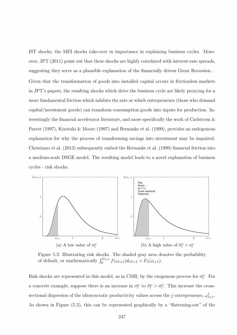
IST shocks, the MEI shocks take-over in importance in explaining business cycles. More-

over, JPT (2011) point out that these shocks are highly correlated with interest-rate spreads,

suggesting they serve as a plausible explanation of the financially driven Great Recession .

Given that the transformation of goods into installed capital occurs in frictionless markets

in JPT’s papers, the resulting shocks which drive the business cycle are likely proxying for a

more fundamental friction which inhibits the rate at which entrepreneurs (those who demand

capital/investment goods) can transform consumption goods into inputs for production. In-

terestingly the financial accelerator literature, and more specifically the work of Carlstrom &

Fuerst (1997), Kiyotaki & Moore (1997) and Bernanke et al. (1999), provides an endogenous

explanation for why the process of transforming savings into investment may be impaired.

Christiano et al. (2013) subsequently embed the Bernanke et al. (1999) financial friction into

a medium-scale DSGE model. The resulting model leads to a novel explanation of business

cycles - risk shocks.

ωt+1 1 2 ωt+1

.5

1

f(ωt+1)

(a) A low value of σωt

ωt+1 1 2 ωt+1

.5

1

f(ωt+1)

RiskShock −

An ⇑ in

Cross−SectionalDispersion

(b) A high value of σωt > σω

t

Figure 5.2: Illustrating risk shocks. The shaded gray area denotes the probability

of default, or mathematically´ ωt+1

0 f(ωt+1)dωt+1 = Ft(ωt+1).

Risk shocks are represented in this model, as in CMR, by the exogenous process for σωt . For

a concrete example, suppose there is an increase in σωt to σωt > σωt . This increase the cross-

sectional dispersion of the idiosyncratic productivity values across the j entrepreneurs, ωjt+1.

As shown in Figure (5.2), this can be represented graphically by a “flattening-out” of the

247

distribution of potential ωt+1 draws from which each entrepreneur j receives their produc-

tivity value. What this means for the entrepreneur is that for a given threshold productivity

value ωt+1 there is now a greater probability the entrepreneur will receive a productivity

draw ωt+1 < ωt+1. More simply, the default probability increases since Ft(ωt+1)> Ft(ωt+1).

Since default is costly due to the costly-state verification the interest rate the bank charges

on unsecured external financing increases to cover the expected higher cost. This induces

the entrepreneur to decrease their borrowing of external funds, leading credit to contract.

The combination of increasing finance premiums, falling credit and ultimately falling output

make risk shocks a prime candidate to explain business cycles. In fact, the inclusion of

finance premiums and credit in the estimation is precisely why CMR find that risk shocks

explain the bulk of the movement in output at business cycle frequencies. They show this

by estimating the model without these financial market variables and find that JPT’s MEI

shocks explain the majority of business cycle movements. The model presented in this paper,

and the foreclosure accelerator mechanism in particular, provides an alternative framework

(which nests these previous models as special cases) to examine the source of business cycle

movements. In contrast to these previous estimation results, I find that home prices play a

significant role in explaining the behavior of finance premiums, credit and output. However,

the debt-contract allows for neutral technology shocks explain the majority of the movements

in GDP without implying empirically inconsistent relationships between financial variables.

Finally, in contrast to CMR (2013), risk shocks play virtually no role in driving real variables

and only explain the high frequency movements in finance premiums.

5.4.1 What are plausible sources of business cycles?

In what follows, I present impulse response functions from the model estimated in this paper,

the model estimated in CMR (2013) and variations of these two models to gain some intuition

for the different econometric conclusions reached in this paper.

248

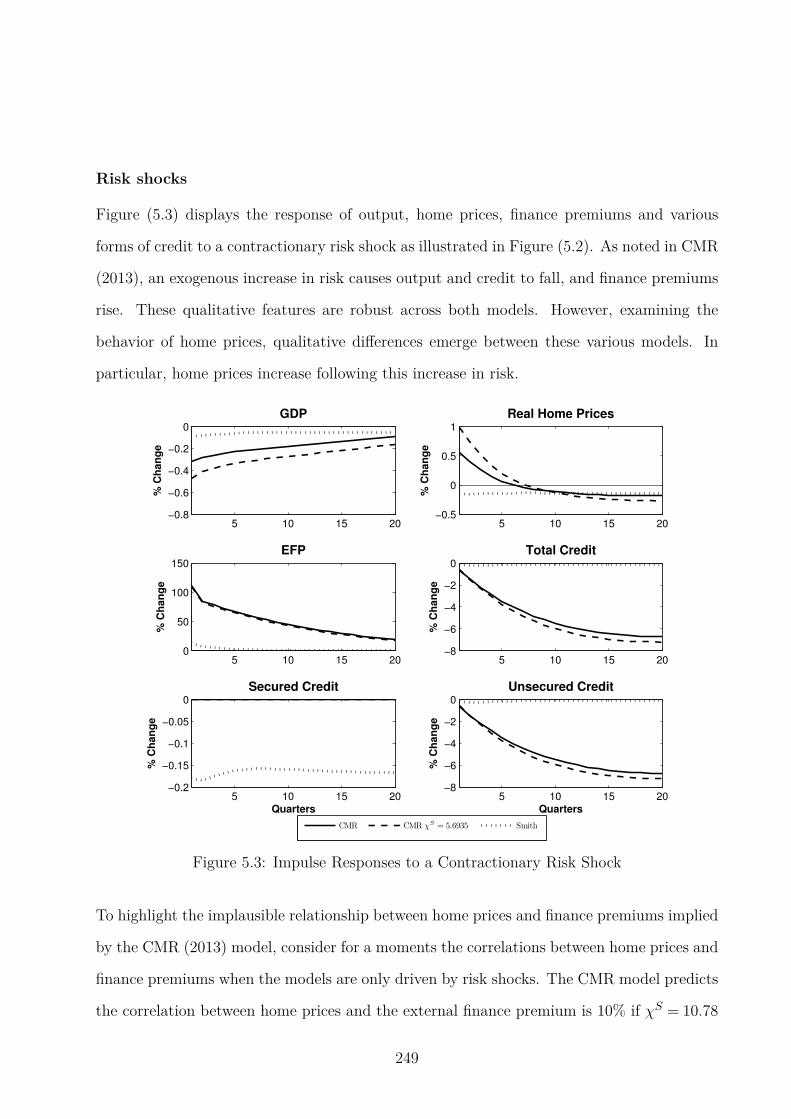
Risk shocks

Figure (5.3) displays the response of output, home prices, finance premiums and various

forms of credit to a contractionary risk shock as illustrated in Figure (5.2). As noted in CMR

(2013), an exogenous increase in risk causes output and credit to fall, and finance premiums

rise. These qualitative features are robust across both models. However, examining the

behavior of home prices, qualitative differences emerge between these various models. In

particular, home prices increase following this increase in risk.

5 10 15 20−0.8

−0.6

−0.4

−0.2

0

GDP

% C

han

ge

5 10 15 20−0.5

0

0.5

1

Real Home Prices%

Ch

an

ge

5 10 15 200

50

100

150

EFP

% C

han

ge

5 10 15 20−8

−6

−4

−2

0

Total Credit

% C

han

ge

5 10 15 20−0.2

−0.15

−0.1

−0.05

0

Quarters

% C

han

ge

Secured Credit

CMR CMR χS = 5.6935 Smith

5 10 15 20−8

−6

−4

−2

0

Unsecured Credit

% C

han

ge

Quarters

Figure 5.3: Impulse Responses to a Contractionary Risk Shock

To highlight the implausible relationship between home prices and finance premiums implied

by the CMR (2013) model, consider for a moments the correlations between home prices and

finance premiums when the models are only driven by risk shocks. The CMR model predicts

the correlation between home prices and the external finance premium is 10% if χS = 10.78

249

and rises to 28% when χS = 5.69. The value in the data over the sample period is 21% and

falls to -61% when computed since 2000. The value in the model estimated in this paper is

-39%. Thus, once home prices are included in the estimation, it seems that risk shocks can

no longer be the primary driver of finance premiums in the CMR model.

Neutral technology shocks

Figure (5.4) displays the response of output, home prices, finance premiums and various

forms of credit to a contractionary TFP technology shock. As expected, a drop in TFP

causes GDP to fall, along with home prices and credit in all models. However, the behavior

of finance premiums is qualitatively different across models, especially across CMR’s model

with alternative values of the curvature of the investment adjustment cost function.

5 10 15 20−1.5

−1

−0.5

0

GDP

% C

ha

ng

e

5 10 15 20−1.5

−1

−0.5

0

Real Home Prices

% C

ha

ng

e

5 10 15 20−5

0

5

10

EFP

% C

ha

ng

e

5 10 15 20−1

−0.5

0

Total Credit

% C

ha

ng

e

5 10 15 20−1.5

−1

−0.5

0

Quarters

% C

ha

ng

e

Secured Credit

CMR CMR χS = 5.6935 Smith

5 10 15 20−0.8

−0.6

−0.4

−0.2

0

Unsecured Credit

% C

ha

ng

e

Quarters

Figure 5.4: Impulse Responses to a Contractionary Technology Shock

On impact, finance premiums rise across all model specifications. However, in the CMR

250

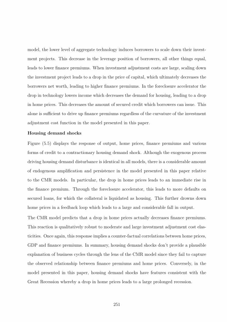
model, the lower level of aggregate technology induces borrowers to scale down their invest-

ment projects. This decrease in the leverage position of borrowers, all other things equal,

leads to lower finance premiums. When investment adjustment costs are large, scaling down

the investment project leads to a drop in the price of capital, which ultimately decreases the

borrowers net worth, leading to higher finance premiums. In the foreclosure accelerator the

drop in technology lowers income which decreases the demand for housing, leading to a drop

in home prices. This decreases the amount of secured credit which borrowers can issue. This

alone is sufficient to drive up finance premiums regardless of the curvature of the investment

adjustment cost function in the model presented in this paper.

Housing demand shocks

Figure (5.5) displays the response of output, home prices, finance premiums and various

forms of credit to a contractionary housing demand shock. Although the exogenous process

driving housing demand disturbance is identical in all models, there is a considerable amount

of endogenous amplification and persistence in the model presented in this paper relative

to the CMR models. In particular, the drop in home prices leads to an immediate rise in

the finance premium. Through the foreclosure accelerator, this leads to more defaults on

secured loans, for which the collateral is liquidated as housing. This further drowns down

home prices in a feedback loop which leads to a large and considerable fall in output.

The CMR model predicts that a drop in home prices actually decreases finance premiums.

This reaction is qualitatively robust to moderate and large investment adjustment cost elas-

ticities. Once again, this response implies a counter-factual correlations between home prices,

GDP and finance premiums. In summary, housing demand shocks don’t provide a plausible

explanation of business cycles through the lens of the CMR model since they fail to capture

the observed relationship between finance premiums and home prices. Conversely, in the

model presented in this paper, housing demand shocks have features consistent with the

Great Recession whereby a drop in home prices leads to a large prolonged recession.

251

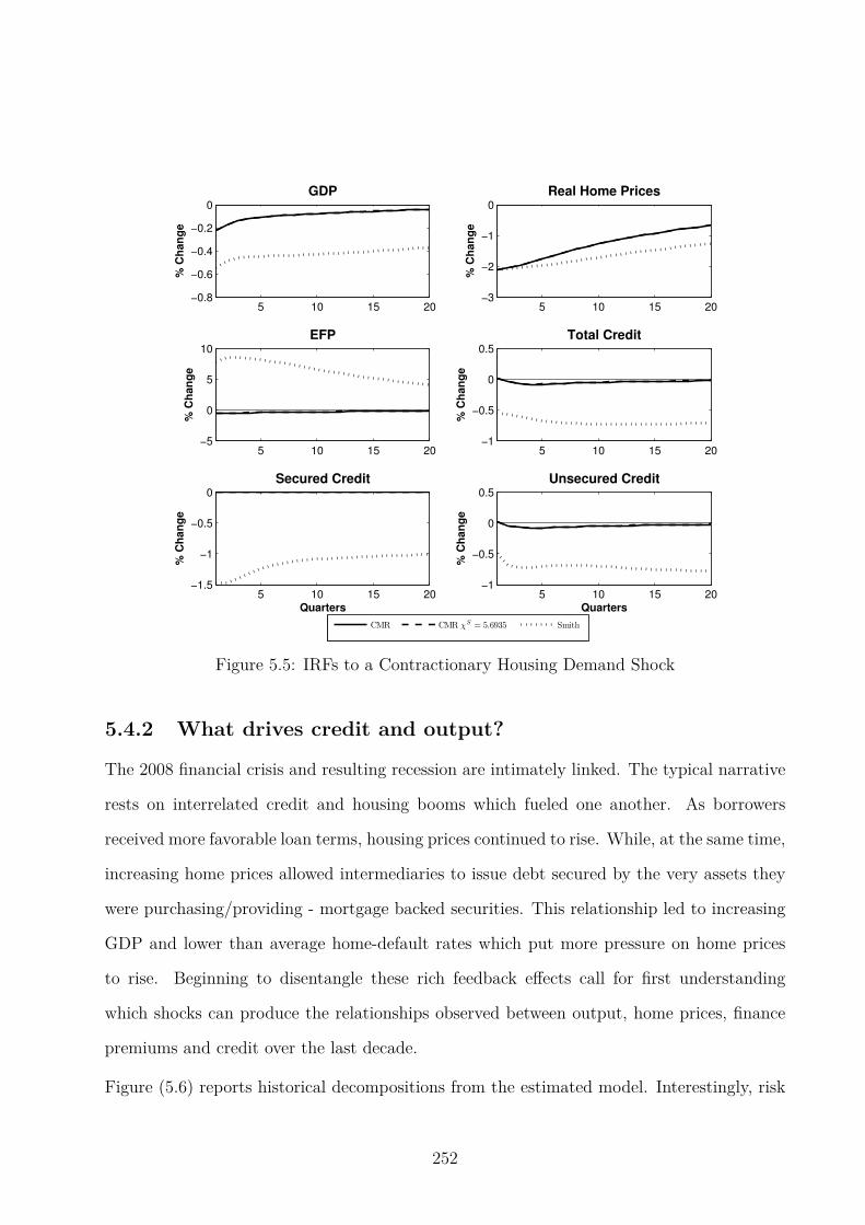
5 10 15 20−0.8

−0.6

−0.4

−0.2

0

GDP%

Ch

an

ge

5 10 15 20−3

−2

−1

0

Real Home Prices

% C

han

ge

5 10 15 20−5

0

5

10

EFP

% C

han

ge

5 10 15 20−1

−0.5

0

0.5

Total Credit

% C

han

ge

5 10 15 20−1.5

−1

−0.5

0

Quarters

% C

han

ge

Secured Credit

CMR CMR χS = 5.6935 Smith

5 10 15 20−1

−0.5

0

0.5

Unsecured Credit

% C

han

ge

Quarters

Figure 5.5: IRFs to a Contractionary Housing Demand Shock

5.4.2 What drives credit and output?

The 2008 financial crisis and resulting recession are intimately linked. The typical narrative

rests on interrelated credit and housing booms which fueled one another. As borrowers

received more favorable loan terms, housing prices continued to rise. While, at the same time,

increasing home prices allowed intermediaries to issue debt secured by the very assets they

were purchasing/providing - mortgage backed securities. This relationship led to increasing

GDP and lower than average home-default rates which put more pressure on home prices

to rise. Beginning to disentangle these rich feedback effects call for first understanding

which shocks can produce the relationships observed between output, home prices, finance

premiums and credit over the last decade.

Figure (5.6) reports historical decompositions from the estimated model. Interestingly, risk

252

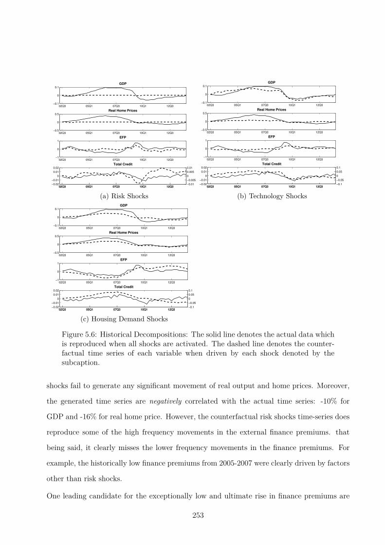
02Q3 05Q1 07Q3 10Q1 12Q3−0.1

0

0.1

GDP

02Q3 05Q1 07Q3 10Q1 12Q3−0.5

0

0.5

Real Home Prices

02Q3 05Q1 07Q3 10Q1 12Q3−1

0

1

EFP

02Q3 05Q1 07Q3 10Q1 12Q3−0.02

−0.01

0

0.01

0.02

Total Credit

02Q3 05Q1 07Q3 10Q1 12Q3−0.01

−0.005

0

0.005

0.01

(a) Risk Shocks

02Q3 05Q1 07Q3 10Q1 12Q3−0.1

0

0.1

GDP

02Q3 05Q1 07Q3 10Q1 12Q3−0.5

0

0.5

Real Home Prices

02Q3 05Q1 07Q3 10Q1 12Q3−1

0

1

EFP

02Q3 05Q1 07Q3 10Q1 12Q3−0.02

−0.01

0

0.01

0.02

Total Credit

02Q3 05Q1 07Q3 10Q1 12Q3−0.1

−0.05

0

0.05

0.1

(b) Technology Shocks

02Q3 05Q1 07Q3 10Q1 12Q3−0.1

0

0.1

GDP

02Q3 05Q1 07Q3 10Q1 12Q3−0.5

0

0.5

Real Home Prices

02Q3 05Q1 07Q3 10Q1 12Q3−1

0

1

EFP

02Q3 05Q1 07Q3 10Q1 12Q3−0.02

−0.01

0

0.01

0.02

Total Credit

02Q3 05Q1 07Q3 10Q1 12Q3−0.1

−0.05

0

0.05

0.1

(c) Housing Demand Shocks

Figure 5.6: Historical Decompositions: The solid line denotes the actual data whichis reproduced when all shocks are activated. The dashed line denotes the counter-factual time series of each variable when driven by each shock denoted by thesubcaption.

shocks fail to generate any significant movement of real output and home prices. Moreover,

the generated time series are negatively correlated with the actual time series: -10% for

GDP and -16% for real home price. However, the counterfactual risk shocks time-series does

reproduce some of the high frequency movements in the external finance premiums. that

being said, it clearly misses the lower frequency movements in the finance premiums. For

example, the historically low finance premiums from 2005-2007 were clearly driven by factors

other than risk shocks.

One leading candidate for the exceptionally low and ultimate rise in finance premiums are

253

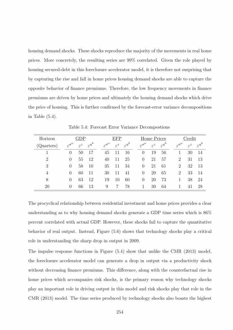
housing demand shocks. These shocks reproduce the majority of the movements in real home

prices. More concretely, the resulting series are 99% correlated. Given the role played by

housing secured-debt in this foreclosure accelerator model, it is therefore not surprising that

by capturing the rise and fall in home prices housing demand shocks are able to capture the

opposite behavior of finance premiums. Therefore, the low frequency movements in finance

premiums are driven by home prices and ultimately the housing demand shocks which drive

the price of housing. This is further confirmed by the forecast-error variance decompositions

in Table (5.4).

Table 5.4: Forecast Error Variance Decompostions

Horizon GDP EFP Home Prices Credit

(Quarters) εσω

εz εηh

εσω

εz εηh

εσω

εz εηh

εσω

εz εηh

1 0 50 17 45 11 16 0 19 56 1 30 14

2 0 55 12 40 11 25 0 21 57 2 31 13

3 0 58 10 35 11 34 0 21 61 2 32 13

4 0 60 11 30 11 41 0 20 65 2 33 14

8 0 63 12 19 10 60 0 20 73 1 38 24

20 0 66 13 9 7 78 1 30 64 1 41 28

The procyclical relationship between residential investment and home prices provides a clear

understanding as to why housing demand shocks generate a GDP time series which is 86%

percent correlated with actual GDP. However, these shocks fail to capture the quantitative

behavior of real output. Instead, Figure (5.6) shows that technology shocks play a critical

role in understanding the sharp drop in output in 2009.

The impulse response functions in Figure (5.4) show that unlike the CMR (2013) model,

the foreclosure accelerator model can generate a drop in output via a productivity shock

without decreasing finance premiums. This difference, along with the counterfactual rise in

home prices which accompanies risk shocks, is the primary reason why technology shocks

play an important role in driving output in this model and risk shocks play that role in the

CMR (2013) model. The time series produced by technology shocks also boasts the highest

254

correlation with credit at 60%. The housing demand series is not far behind at 48% while

the risk shocks time series of credit is only 23% correlated with the actual time series of

credit.

5.4.3 Was the Great Recession the efficient response to technology

shocks?

The above findings suggest that technology shocks played a significant role in shaping the

path of output and credit in the wake of the great recession. In the spirit of Kydland &

Prescott (1982), this calls into question the extent to which countercyclical policy was nec-

essary in response to the recent recession. To assess the extent to which the fall in output

was ‘inefficient,’ and hence should be offset by policy makers, I compute the financial fric-

tions output gap. More specifically, I feed the filtered technology shocks through the model

presented in this paper and an identical model without financial frictions. The frictionless

model is identical, except the entrepreneur’s first order condition is replaced by a typical

Euler equation for capital. I then compute the difference between GDP in the full model

and the frictionless model - the financial frictions output gap.

Figure (5.7) illustrates the results of this exercise which are also repeated by feeding all

non-financial shocks through each model so that the number of shocks is always identical in

both models. Two immediate conclusions emerge from this exercise. First, the majority of

the fall in the output gap at the onset of the recession was due to technology shocks. Second,

the adverse technology shocks are primarily transferred through the financial sector, which

results in a large negative output gap, even when technology shocks are the only source of

the business cycle. Thus, the endogenous financial frictions, amplify and propagated the

downturn, therefore justifying considerable intervention into financial markets to limit the

inefficiencies associated with the recession.

255

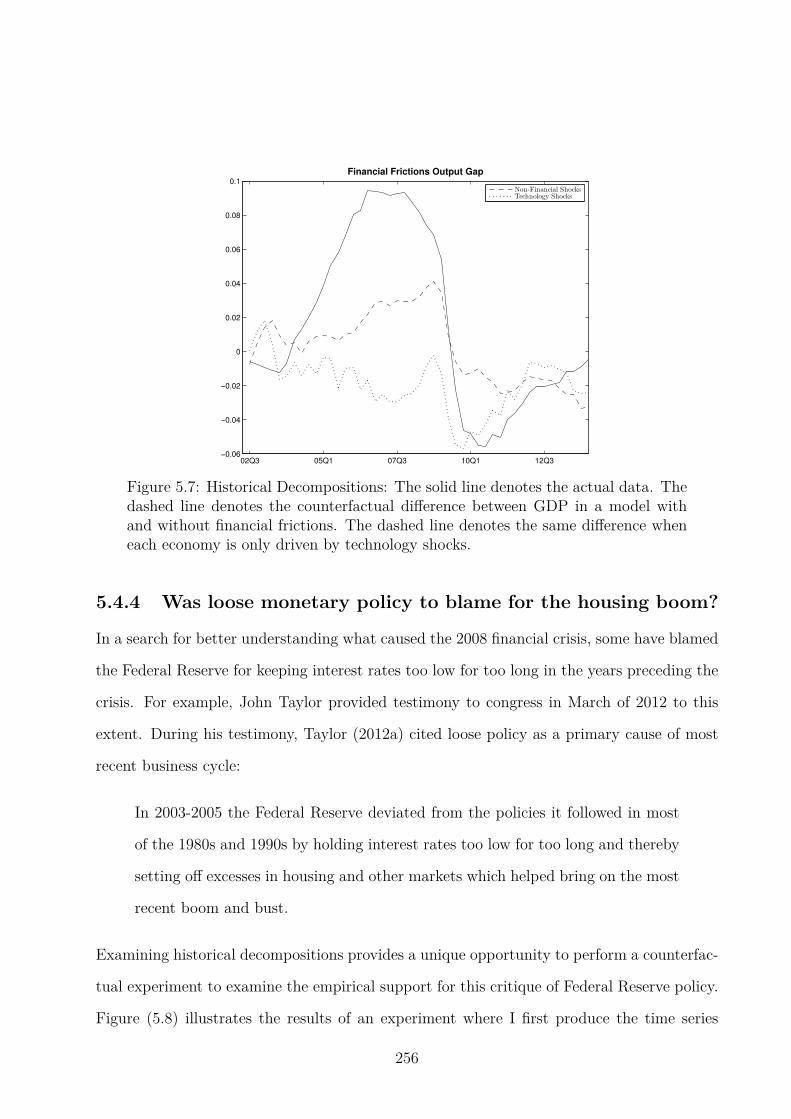
02Q3 05Q1 07Q3 10Q1 12Q3−0.06

−0.04

−0.02

0

0.02

0.04

0.06

0.08

0.1

Financial Frictions Output Gap

Non-Financial ShocksTechnology Shocks

Figure 5.7: Historical Decompositions: The solid line denotes the actual data. Thedashed line denotes the counterfactual difference between GDP in a model withand without financial frictions. The dashed line denotes the same difference wheneach economy is only driven by technology shocks.

5.4.4 Was loose monetary policy to blame for the housing boom?

In a search for better understanding what caused the 2008 financial crisis, some have blamed

the Federal Reserve for keeping interest rates too low for too long in the years preceding the

crisis. For example, John Taylor provided testimony to congress in March of 2012 to this

extent. During his testimony, Taylor (2012a) cited loose policy as a primary cause of most

recent business cycle:

In 2003-2005 the Federal Reserve deviated from the policies it followed in most

of the 1980s and 1990s by holding interest rates too low for too long and thereby

setting off excesses in housing and other markets which helped bring on the most

recent boom and bust.

Examining historical decompositions provides a unique opportunity to perform a counterfac-

tual experiment to examine the empirical support for this critique of Federal Reserve policy.

Figure (5.8) illustrates the results of an experiment where I first produce the time series

256

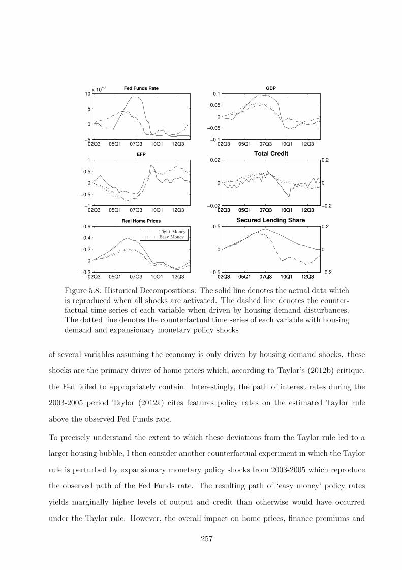
02Q3 05Q1 07Q3 10Q1 12Q3−5

0

5

10x 10

−3 Fed Funds Rate

02Q3 05Q1 07Q3 10Q1 12Q3−0.1

−0.05

0

0.05

0.1GDP

02Q3 05Q1 07Q3 10Q1 12Q3−1

−0.5

0

0.5

1EFP

02Q3 05Q1 07Q3 10Q1 12Q3−0.02

0

0.02

02Q3 05Q1 07Q3 10Q1 12Q3−0.2

0

0.2

Total Credit

02Q3 05Q1 07Q3 10Q1 12Q3−0.2

0

0.2

0.4

0.6Real Home Prices

Tight MoneyEasy Money

02Q3 05Q1 07Q3 10Q1 12Q3−0.5

0

0.5

02Q3 05Q1 07Q3 10Q1 12Q3−0.2

0

0.2

Secured Lending Share

Figure 5.8: Historical Decompositions: The solid line denotes the actual data whichis reproduced when all shocks are activated. The dashed line denotes the counter-factual time series of each variable when driven by housing demand disturbances.The dotted line denotes the counterfactual time series of each variable with housingdemand and expansionary monetary policy shocks

of several variables assuming the economy is only driven by housing demand shocks. these

shocks are the primary driver of home prices which, according to Taylor’s (2012b) critique,

the Fed failed to appropriately contain. Interestingly, the path of interest rates during the

2003-2005 period Taylor (2012a) cites features policy rates on the estimated Taylor rule

above the observed Fed Funds rate.

To precisely understand the extent to which these deviations from the Taylor rule led to a

larger housing bubble, I then consider another counterfactual experiment in which the Taylor

rule is perturbed by expansionary monetary policy shocks from 2003-2005 which reproduce

the observed path of the Fed Funds rate. The resulting path of ‘easy money’ policy rates

yields marginally higher levels of output and credit than otherwise would have occurred

under the Taylor rule. However, the overall impact on home prices, finance premiums and

257

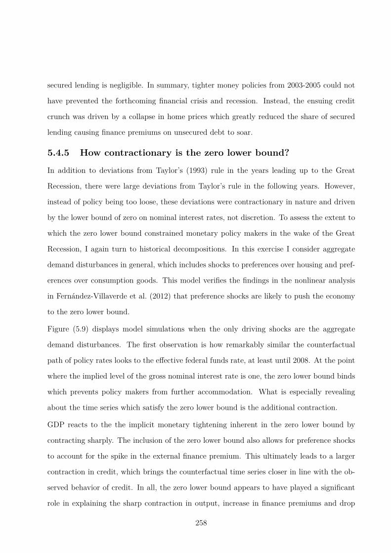
secured lending is negligible. In summary, tighter money policies from 2003-2005 could not

have prevented the forthcoming financial crisis and recession. Instead, the ensuing credit

crunch was driven by a collapse in home prices which greatly reduced the share of secured

lending causing finance premiums on unsecured debt to soar.

5.4.5 How contractionary is the zero lower bound?

In addition to deviations from Taylor’s (1993) rule in the years leading up to the Great

Recession, there were large deviations from Taylor’s rule in the following years. However,

instead of policy being too loose, these deviations were contractionary in nature and driven

by the lower bound of zero on nominal interest rates, not discretion. To assess the extent to

which the zero lower bound constrained monetary policy makers in the wake of the Great

Recession, I again turn to historical decompositions. In this exercise I consider aggregate

demand disturbances in general, which includes shocks to preferences over housing and pref-

erences over consumption goods. This model verifies the findings in the nonlinear analysis

in Fernández-Villaverde et al. (2012) that preference shocks are likely to push the economy

to the zero lower bound.

Figure (5.9) displays model simulations when the only driving shocks are the aggregate

demand disturbances. The first observation is how remarkably similar the counterfactual

path of policy rates looks to the effective federal funds rate, at least until 2008. At the point

where the implied level of the gross nominal interest rate is one, the zero lower bound binds

which prevents policy makers from further accommodation. What is especially revealing

about the time series which satisfy the zero lower bound is the additional contraction.

GDP reacts to the the implicit monetary tightening inherent in the zero lower bound by

contracting sharply. The inclusion of the zero lower bound also allows for preference shocks

to account for the spike in the external finance premium. This ultimately leads to a larger

contraction in credit, which brings the counterfactual time series closer in line with the ob-

served behavior of credit. In all, the zero lower bound appears to have played a significant

role in explaining the sharp contraction in output, increase in finance premiums and drop

258

02Q3 05Q1 07Q3 10Q1 12Q3−0.015

−0.01

−0.005

0

0.005

0.01

Fed Funds Rate

No ZLBBinding ZLB

02Q3 05Q1 07Q3 10Q1 12Q3−0.1

−0.05

0

0.05

0.1

GDP

02Q3 05Q1 07Q3 10Q1 12Q3−1

−0.5

0

0.5

1

EFP

02Q3 05Q1 07Q3 10Q1 12Q3−0.02

0

0.02

02Q3 05Q1 07Q3 10Q1 12Q3−0.2

0

0.2

Total Credit

Figure 5.9: Historical Decompositions: The solid line denotes the actual data whichis reproduced when all shocks are activated. The dashed line denotes the counter-factual time series of each variable when driven by housing/consumption demanddisturbances. The dotted line is the same time series when the ZLB binds.

in credit. Risk shocks are noticeably absent from this explanation as they don’t drive the

economy to the zero lower bound. Figure (5.6) reveals that risk shocks were actually expan-

sionary from 2009 onwards. As counter-intuitive as this seems, it is likely the result of the

unconventional policy actions taken by the Federal Reserve and the TARP equity injections

which decreased systemic risk by stabilizing large financial firms.

5.5 Conclusion

Despite the fact that most narratives of the 2008 financial crisis and ensuing Great Recession

feature housing markets and secured debt markets, current equilibrium models don’t typically

feature both (and often feature neither) markets. The implication is a large gap between

the narrative description of the worst postwar recession and the sources of the downturn

attributed by structural equilibrium models. This paper bridges that gap. By including

259

integrated housing and financial markets in an otherwise standard medium scale DSGE

model, I provide an interpretation of the last decade that is more consistent with the casual

observation that housing and debt markets are highly integrated.

Unlike the recent findings of Christiano et al. (2013), I find that risk shocks account for es-

sentially none of the variation in real GDP. These shocks essentially capture high frequency

movements in finance premiums but otherwise have little predictive power regarding out-

put, home prices, finance premiums and credit. Instead, housing demand and total factor

productivity disturbances explain the bulk of the variation of housing, financial and goods

markets. This is due in large part to the novel debt contract which augments the finan-

cial accelerator with a foreclosure accelerator mechanism. This framework is better suited

to capture the observed relationships between home prices, finance premiums and output.

Although technology shocks in frictionless models imply there is no role for countercyclical

policy, I show the endogenous behavior of the modeled financial frictions played a significant

role in transmitting the technology shocks to the broader economy. The implication being

that countercyclical policy, especially intervention into financial markets, is well justified.

Along these same policy lines, I find the claim that the Federal Reserve kept interest rate

too low for too long and fueled the housing bubble has little empirical footing. Instead,

the housing expansion was largely driven by the interaction of exogenous housing demand

disturbances and the foreclosure accelerator mechanism. Counterfactual simulations show

that tighter monetary policy would have had a marginal effect on most variables. Conversely,

the deviations from the interest rate rule following the Great Recession played a significant

role in the large contraction of output and the spike in finance premiums in 2008-2009.

260

References

Bernanke, B. S., Gertler, M., & Gilchrist, S. (1999). The financial accelerator in a quan-

titative business cycle framework. In J. B. Taylor & M. Woodford (Eds.), Handbook of

Macroeconomics, volume 1 of Handbook of Macroeconomics chapter 21, (pp. 1341–1393).

Elsevier.

Calvo, G. A. (1983). Staggered prices in a utility-maximizing framework. Journal of Mone-

tary Economics, 12(3), 383–398.

Carlstrom, C. T. & Fuerst, T. S. (1997). Agency costs, net worth, and business fluctuations:

A computable general equilibrium analysis. American Economic Review, 87(5), 893–910.

Christiano, L., Motto, R., & Rostagno, M. (2013). Risk Shocks. NBER Working Papers

18682, National Bureau of Economic Research, Inc.

Christiano, L. J., Eichenbaum, M., & Evans, C. L. (2005). Nominal rigidities and the dynamic

effects of a shock to monetary policy. Journal of Political Economy, 113(1), 1–45.

Davis, M. A. & Heathcote, J. (2005). Housing and the business cycle. International Economic

Review, 46(3), 751–784.

Erceg, C. J., Henderson, D. W., & Levin, A. T. (2000). Optimal monetary policy with

staggered wage and price contracts. Journal of Monetary Economics, 46(2), 281–313.

Fernández-Villaverde, J., Gordon, G., Guerrón-Quintana, P. A., & Rubio-Ramírez, J. (2012).

261

Nonlinear Adventures at the Zero Lower Bound. NBER Working Papers 18058, National

Bureau of Economic Research, Inc.

Fuhrer, J. C. (2000). Habit Formation in Consumption and Its Implications for Monetary-

Policy Models. American Economic Review, 90(3), 367–390.

Iacoviello, M. (2005). House prices, borrowing constraints, and monetary policy in the

business cycle. American Economic Review, 95(3), 739–764.

Iacoviello, M. & Neri, S. (2010). Housing market spillovers: Evidence from an estimated

dsge model. American Economic Journal: Macroeconomics, 2(2), 125–64.

Ireland, P. N. (2004a). Money’s role in the monetary business cycle. Journal of Money,

Credit and Banking, 36(6), 969–83.

Ireland, P. N. (2004b). Technology shocks in the new keynesian model. The Review of

Economics and Statistics, 86(4), 923–936.

Justiniano, A., Primiceri, G., & Tambalotti, A. (2010). Investment shocks and business

cycles. Journal of Monetary Economics, 57(2), 132–145.

Justiniano, A., Primiceri, G., & Tambalotti, A. (2011). Investment Shocks and the Relative

Price of Investment. Review of Economic Dynamics, 14(1), 101–121.

Keen, B. & Wang, Y. (2007). What is a realistic value for price adjustment costs in new

keynesian models? Applied Economics Letters, 14(11), 789–793.

Kiyotaki, N. & Moore, J. (1997). Credit cycles. Journal of Political Economy, 105(2), 211–48.

Kydland, F. E. & Prescott, E. C. (1982). Time to build and aggregate fluctuations. Econo-

metrica, 50(6), 1345–70.

Rotemberg, J. J. (1982). Sticky prices in the united states. Journal of Political Economy,

90(6), 1187–1211.

262

Smets, F. & Wouters, R. (2007). Shocks and Frictions in US Business Cycles: A Bayesian

DSGE Approach. American Economic Review, 97(3), 586–606.

Taylor, J. B. (1993). Discretion versus policy rules in practice. Carnegie-Rochester Confer-

ence Series on Public Policy, 39(1), 195–214.

Taylor, J. B. (2012a). Monetary Policy Going Forward: Why a Sound Dollar Boosts Growth

and Employment. Testimony before the joint economic committee.

Taylor, J. B. (2012b). Monetary Policy Rules Work and Discretion Doesn’t: A Tale of Two

Eras. Journal of Money, Credit and Banking, 44(6), 1017–1032.

Townsend, R. M. (1979). Optimal contracts and competitive markets with costly state

verification. Journal of Economic Theory, 21(2), 265–293.

263

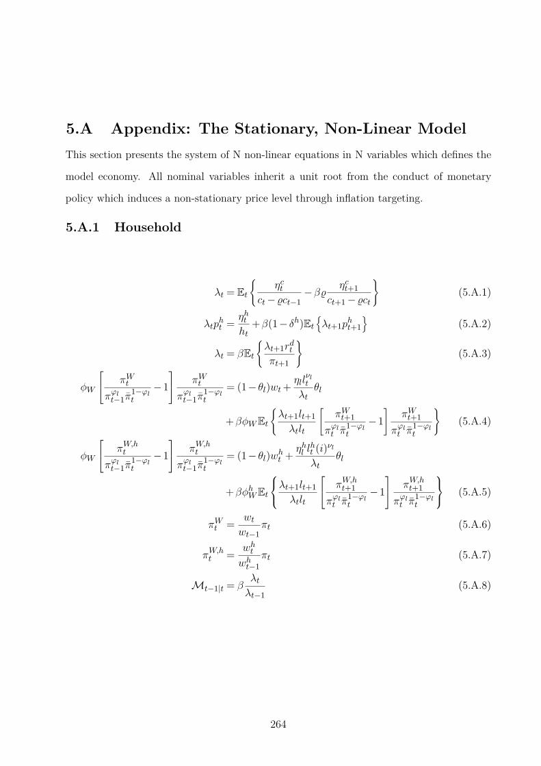
5.A Appendix: The Stationary, Non-Linear Model

This section presents the system of N non-linear equations in N variables which defines the

model economy. All nominal variables inherit a unit root from the conduct of monetary

policy which induces a non-stationary price level through inflation targeting.

5.A.1 Household

λt = Et

ηctct−ct−1

−βηct+1

ct+1 −ct

(5.A.1)

λtpht =

ηhtht

+β(1− δh)Et

λt+1pht+1

(5.A.2)

λt = βEt

λt+1rdt

πt+1

(5.A.3)

φW

πWt

πϕlt−1π

1−ϕlt

−1

πWt

πϕlt−1π

1−ϕlt

= (1− θl)wt+ηll

νlt

λtθl

+βφWEt

λt+1lt+1

λtlt

[

πWt+1

πϕlt π

1−ϕlt

−1

]

πWt+1

πϕlt π

1−ϕlt

(5.A.4)

φW

πW,ht

πϕlt−1π

1−ϕlt

−1

πW,ht

πϕlt−1π

1−ϕlt

= (1− θl)wht +

ηhl lht (i)νl

λtθl

+βφhWEt

λt+1lt+1

λtlt

πW,ht+1

πϕlt π

1−ϕlt

−1

πW,ht+1

πϕlt π

1−ϕlt

(5.A.5)

πWt =wtwt−1

πt (5.A.6)

πW,ht =whtwht−1

πt (5.A.7)

Mt−1|t = βλtλt−1

(5.A.8)

264

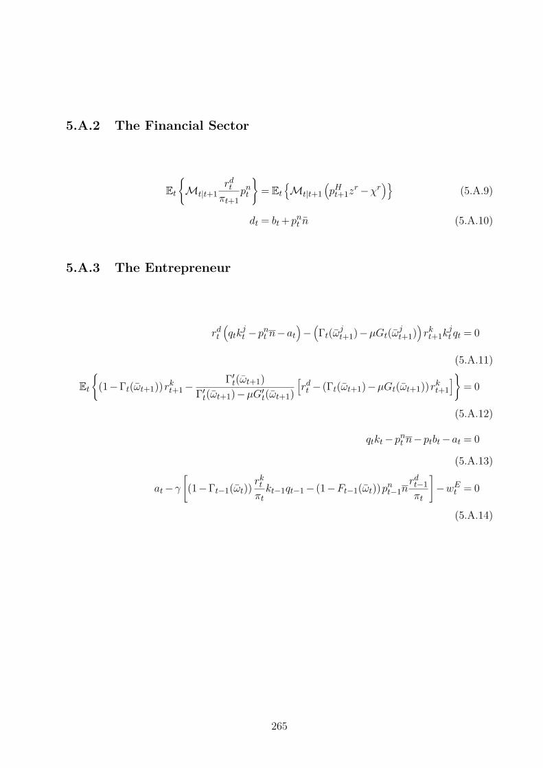
5.A.2 The Financial Sector

Et

Mt|t+1rdtπt+1

pnt

= Et

Mt|t+1

(

pHt+1zr −χr

)

(5.A.9)

dt = bt+pnt n (5.A.10)

5.A.3 The Entrepreneur

rdt(

qtkjt −pnt n−at

)

−(

Γt(ωjt+1)−µGt(ω

jt+1)

)

rkt+1kjt qt = 0

(5.A.11)

Et

(1−Γt(ωt+1))rkt+1 − Γ′t(ωt+1)

Γ′t(ωt+1)−µG′

t(ωt+1)

[

rdt − (Γt(ωt+1)−µGt(ωt+1))rkt+1

]

= 0

(5.A.12)

qtkt−pnt n−ptbt−at = 0

(5.A.13)

at−γ

[

(1−Γt−1(ωt))rktπtkt−1qt−1 − (1−Ft−1(ωt))p

nt−1n

rdt−1

πt

]

−wEt = 0

(5.A.14)

265

5.A.4 Relevant Distributions for the Entrepreneurs

xt+1 =ln(ωt+1)+ .5(σωt )2

σωt(5.A.15)

Gt(ωt+1) = ΦN (xt+1 −σωt ) (5.A.16)

Γt(ωt+1) = ΦN (xt+1 −σωt )+ ωt+1(1−ΦN (xt+1)) (5.A.17)

G′

t(ωt+1) =

(

1

σωt√

2π

)

e−x2t+1/2 (5.A.18)

Γ′

t(ωt+1) = 1−ΦN (xt+1) (5.A.19)

Ft(ωt+1) = ΦN (xt+1) (5.A.20)

υt−1(ωt) =Gt−1(ωt)rktπtqt−1kt−1 (5.A.21)

5.A.5 The Wholesale Goods Producers

yt = zt(kt−1)α(l′

t)1−α (5.A.22)

l′

t = l1−αE

t (5.A.23)

wt = pWt (1−α)(1−αE)ytlt

(5.A.24)

wEt = pWt (1−α)αEyt (5.A.25)

mpkt = αytkt−1

(5.A.26)

rkt =utmp

kt pWt −a(ut)+(1− δk)qt

qt−1πt (5.A.27)

a(ut) =mpk

χa

[

eχa(ut−1) −1

]

(5.A.28)

mpkt =mpkeχa(ut−1) (5.A.29)

266

5.A.6 Retail Goods Producers

φ

πt

πϕt−1π1−ϕt

−1

πt

πϕt−1π1−ϕt

= θpWt − (θ−1) (5.A.30)

+φEt

yt+1Mt,t+1

ytMt,t

[

πt+1

πϕt π1−ϕt

−1

]

πt+1

πϕt π1−ϕt

5.A.7 New Housing Production

hnewt = zht (lht )(1−αh) (5.A.31)

wht = pht (1−αh)hnewt

lht(5.A.32)

5.A.8 Investment Goods Production

pit =1

zit(5.A.33)

5.A.9 Capital Goods Production

kt =

(

it−S

(

it

zkt kt−1

)

zkt kt−1

)

+(1− δk)kt−1 (5.A.34)

S

(

it

zkt kt−1

)

=χS

2

[

it

zkt kt−1− δk

]2

(5.A.35)

qt =pit

1−S′(

itzk

t kt

) (5.A.36)

267

5.A.10 Monetary Policy

rdtrd

=

(

rdt−1

rd

)ρr(

πtπt

)ψπ(

ytyt−1

)ψy

eεrt (5.A.37)

5.A.11 Market Clearing

ht = hnewt +Ft−1(ωt)zrn+(1− δh)ht−1 (5.A.38)

yt = ct+pitit+Ft−1(ωt)χrn+µυt−1(ωt)+a(ut)+act (5.A.39)

act =φ

2

πt

πϕt−1π1−ϕt

−1

2

yt+φW2

πWt

πϕlt−1π

1−ϕlt

−1

2

lt+φW2

πW

h

t

πϕlt−1π

1−ϕlt

−1

2

lht (5.A.40)

268

5.A.12 Exogenous Shocks

ln(ηct ) = ρηcln(ηct−1)+ εηc

t (5.A.41)

ln(ηht ) = (1−ρηh)ln(ηh)+ρηhln(ηht−1)+ εηh

t (5.A.42)

ln(ηl,t) = (1−ρηl)ln(ηl)+ρηl

ln(ηl,t−1)+ εηlt (5.A.43)

ln(ηhl,t) = (1−ρηhl)ln(ηhl )+ρηh

lln(ηhl,t−1)+ εηl

t (5.A.44)

ln(χrt ) = (1−ρχr)χrρχr ln(χrt−1)+ εχr

t (5.A.45)

ln(σωt ) = (1−ρσω)ln(σω)+ρσω ln(σωt−1)+ εσω

t (5.A.46)

ln(zt) = (1−ρz)z+ρzln(zt−1)+ εzt (5.A.47)

ln(θt) = (1−ρθ)θ+ρθln(θt−1)+ εθt (5.A.48)

ln(zht ) = (1−ρzh)ln(zh)+ρzhln(zht−1)+ εzh

t (5.A.49)

ln(zit) = ρizln(zit−1)+ εzi

t (5.A.50)

ln(zkt ) = ρkz ln(zkt−1)+ εzk

t (5.A.51)

ln(πt) = (1−ρπ)π+ρπln(πt−1)+ επt (5.A.52)

ln(ǫrt ) = εrt (5.A.53)

ln(ǫr,newst ) = ρnewsr ln(ǫr,newst−1 )+ ǫr,newst−4 (5.A.54)

269