1

Monetary Policy and MacroprudentialPolicy: Rivals or Teammates?

CNB Working Papers 2016/06

Simona Malovana Jan Frait

CNB Research Open Day, May 15th 2017

The views expressed in this paper are those of the authorsand not necessarily those of the Czech National Bank.

1 Motivation and research questions

2 Empirical framework

3 Results

4 Discussion and conclusions

2

Outline

•Monetary and macroprudential policy not independent, affect boththe monetary and credit conditions via their effect on credit growth(Borio, 2014)•Macroprudential tools becoming used more actively & prolonged

period of very accommodative monetary easing• Building up of vulnerabilities?• A highly accommodative monetary policy can increase risks to

financial stability and lead to a buildup of financial vulnerabilities (e.gexcessive credit growth) - negative effect on real economy in the future(Adrian & Liang, 2014; Lowe & Borio, 2002)

• Policy coordination? Proper policy mix?• Coordination difficult - different probabilities of failure to fulfil the two

main objectives (Adrian & Liang, 2014)• Risks to price stability materialize in short-to-medium run, risks to

financial stability in medium-to-long run

3

Motivation

•Objective: to study the extent to what monetary policy maycontribute to a buildup of financial vulnerabilities and the effect ofmacroprudential capital regulation on macroeconomy and creditcycle•What is the effect of monetary policy on credit cycle and banks’ capital

ratio?• Does this effect change over time?•What are international spillovers to Czech credit cycle and banks’

capital?• Does monetary policy affect risk-taking behavior of banks?•What is the effect of macroprudential capital policy tightening on credit

cycle and real economy?• How?• Empirical framework at the macro level – panel VAR with time-varying

coefficients estimated using Bayesian approach• Empirical framework at the micro level – simple panel regression

model estimated using GMM4

Objective and research questions

• Panel VAR model with time-varying coefficients• to study possible spillover from abroad to Czech economy,• to capture mutual interdependencies,• to compare the dynamics of Czech and closely related economies.• High dimensional problem reduced to low dimensional using

common factors as proposed by Canova & Ciccarelli (2009)• The factors capture components in the coefficient vector which are

common in some way, for example, across units, variables or lags• Final combination of common factors chosen based on the

maximum marginal log-likelihood•Model is estimated using Bayesian approach with standard set of

priors (Normal-inverse-Wishart distribution)• Shock identified using Cholesky decomposition, benchmark

ordering subjected to a number of robustness checks

5

Empirical framework at the macro level

• 6 countries – CZ, DE, FR, IT, AT, BE• CZ and closely related countries (through trade and financial links)• 70% of total euro area banks’ assets, 72% of euro area GDP• 5 variables – credit of private non-financial sector to GDP, banks’

non-risk-weighted capital-to-asset ratio, real GDP, CPI, monetarypolicy proxy• Quarter-on-quarter growth rates, annualized, scaled by s.d.• Time period – 1Q/2000 to 3Q/2015

Monetary Condition Index• ZLB, unconventional measures - alternative index estimated• Dynamic factor analysis, the EM algorithm, set of variables related

to conventional and unconventional monetary policy in CZ and EA• Robust to different specifications

6

Data at the macro level

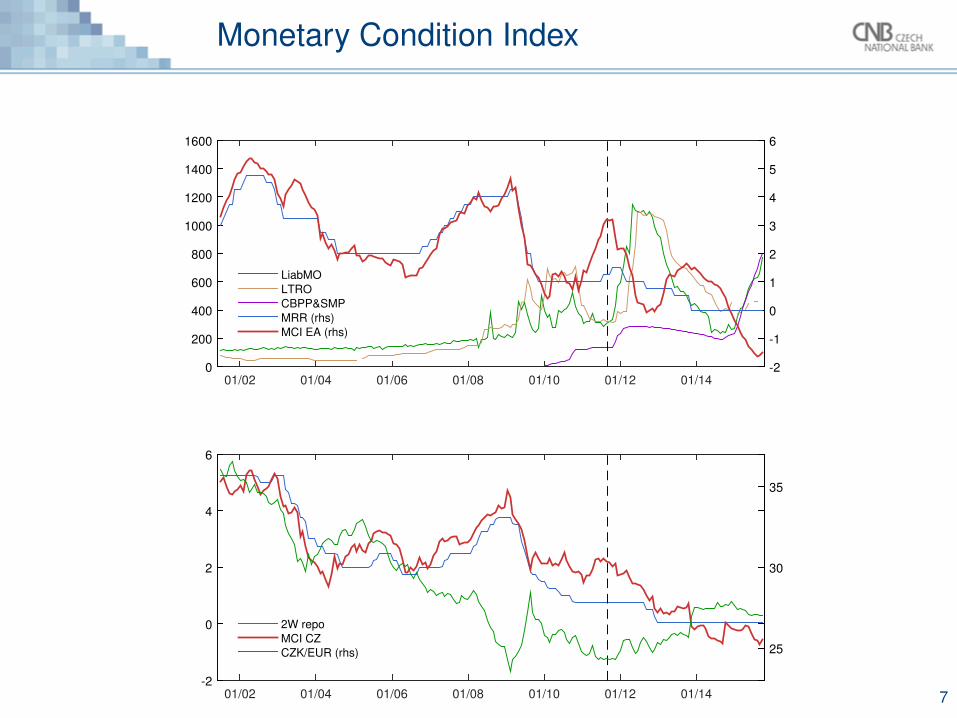
01/02 01/04 01/06 01/08 01/10 01/12 01/140

200

400

600

800

1000

1200

1400

1600

-2

-1

0

1

2

3

4

5

6

LiabMO

LTRO

CBPP&SMP

MRR (rhs)

MCI EA (rhs)

01/02 01/04 01/06 01/08 01/10 01/12 01/14-2

0

2

4

6

25

30

35

2W repo

MCI CZ

CZK/EUR (rhs)

7

Monetary Condition Index

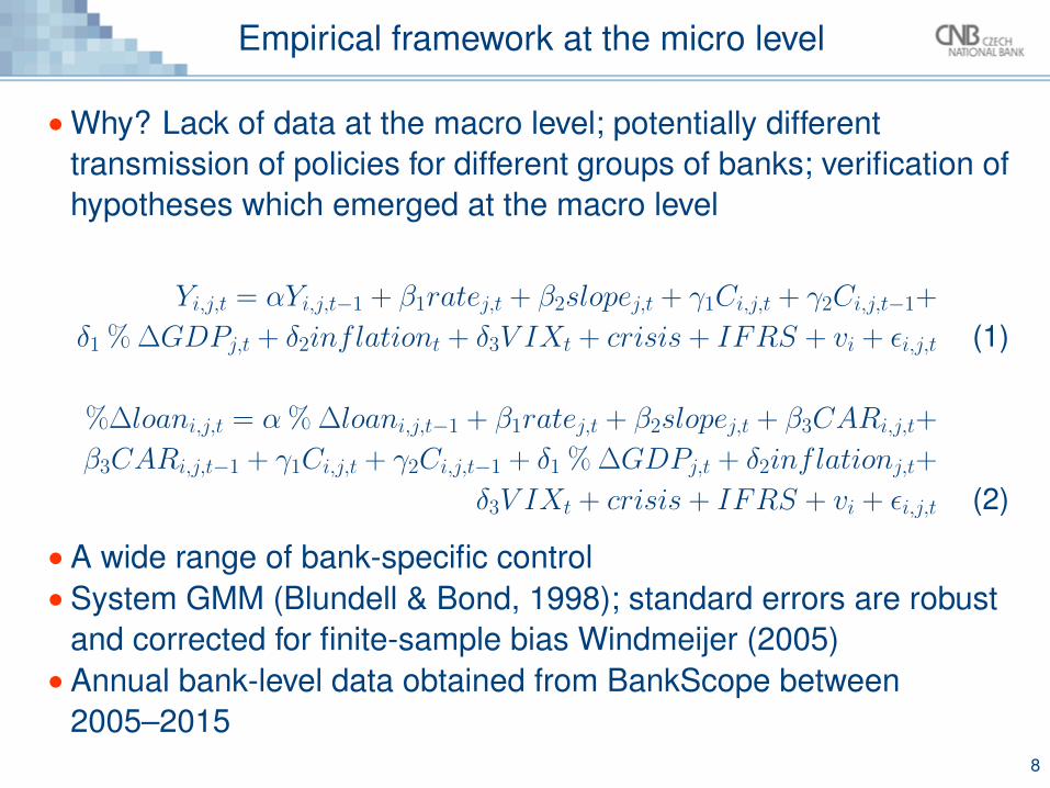
•Why? Lack of data at the macro level; potentially differenttransmission of policies for different groups of banks; verification ofhypotheses which emerged at the macro level

Yi,j,t = αYi,j,t−1 + β1ratej,t + β2slopej,t + γ1Ci,j,t + γ2Ci,j,t−1+

δ1 % ∆GDPj,t + δ2inflationt + δ3V IXt + crisis + IFRS + vi + εi,j,t (1)

%∆loani,j,t = α % ∆loani,j,t−1 + β1ratej,t + β2slopej,t + β3CARi,j,t+

β3CARi,j,t−1 + γ1Ci,j,t + γ2Ci,j,t−1 + δ1 % ∆GDPj,t + δ2inflationj,t+

δ3V IXt + crisis + IFRS + vi + εi,j,t (2)

• A wide range of bank-specific control• System GMM (Blundell & Bond, 1998); standard errors are robust

and corrected for finite-sample bias Windmeijer (2005)• Annual bank-level data obtained from BankScope between

2005–20158

Empirical framework at the micro level

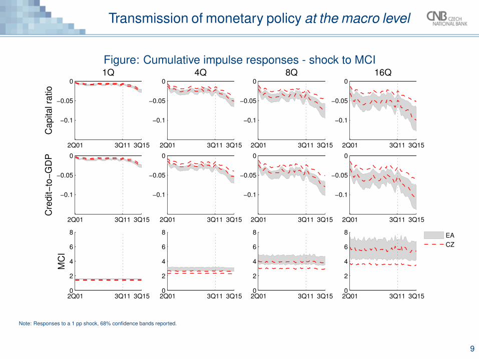
Figure: Cumulative impulse responses - shock to MCI

2Q01 3Q11 3Q15

−0.1

−0.05

0

Capital ra

tio

1Q

2Q01 3Q11 3Q15

−0.1

−0.05

0

4Q

2Q01 3Q11 3Q15

−0.1

−0.05

0

8Q

2Q01 3Q11 3Q15

−0.1

−0.05

0

16Q

2Q01 3Q11 3Q15

−0.1

−0.05

0

Cre

dit−

to−

GD

P

2Q01 3Q11 3Q15

−0.1

−0.05

0

2Q01 3Q11 3Q15

−0.1

−0.05

0

2Q01 3Q11 3Q15

−0.1

−0.05

0

2Q01 3Q11 3Q150

2

4

6

8

MC

I

2Q01 3Q11 3Q150

2

4

6

8

2Q01 3Q11 3Q150

2

4

6

8

2Q01 3Q11 3Q150

2

4

6

8

EA

CZ

Note: Responses to a 1 pp shock, 68% confidence bands reported.

9

Transmission of monetary policy at the macro level

• Transmission through negative short-term impact on profitabilityand positive impact on loan loss provisions• Flattening of the yield curve; imperfect pass-through; reduced

margins – net interest revenues – retained earnings• Higher loan losses and recognised loan loss provisions – reduced

retained earnings (Borio et al. (2015) and Borio & Zhu (2014))• Increase debt service burdens and consequently probabilities of

default (stock of loans)• Increase the perceived riskiness of new clients and induce less

risk-taking on new loans

10

Effect of shock to MCI on bank capital ratio

Controlling for macroeconomic conditions and bank characteristics, weshould expect• a negative relationship between bank profitability and the

short-term interest rate (consistently with loan pricing frictions),• a positive relationship between loan loss provisions and the

short-term interest rate (impact of higher interest rates on defaults;potential forward-looking provisioning),• a positive relationship between profitability and equity to total

assets (impact on retained earnings which are part of the equitycapital),• a negative relationship between equity to risk-weighted assets and

the short-term interest rate (impact of higher interest rates onbanks perception and measuring of risks – impact on estimates ofprobability of default, loss given default and volatilities).

11

Testable hypotheses

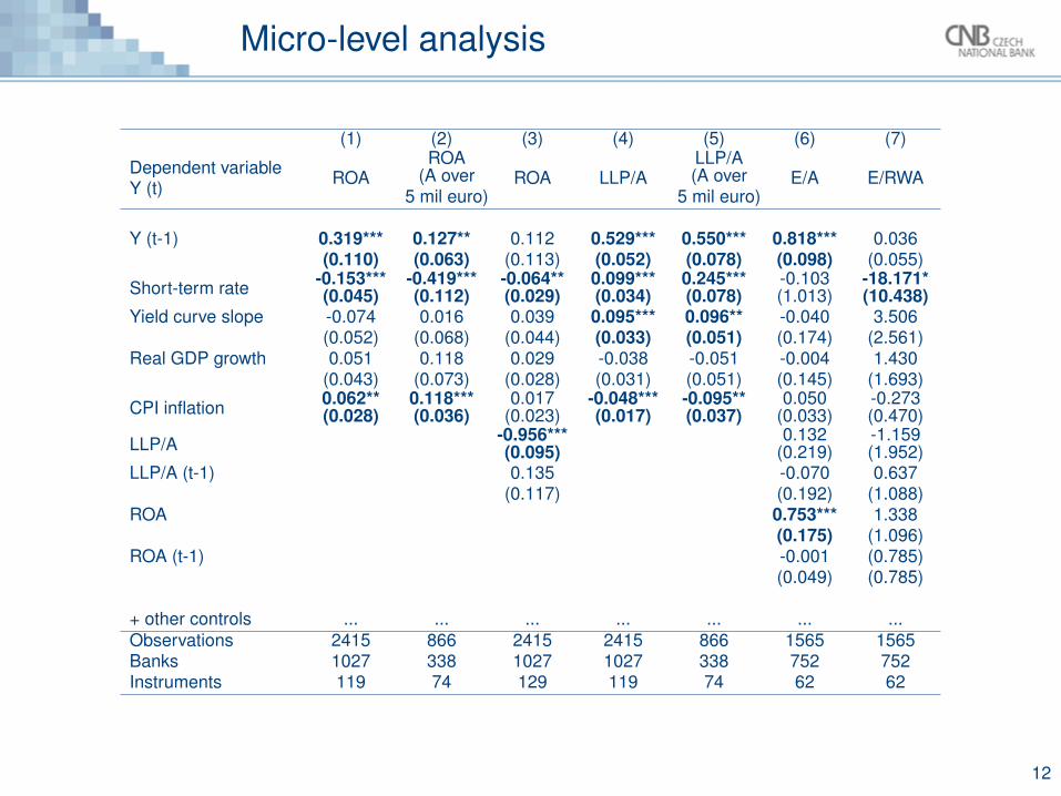
(1) (2) (3) (4) (5) (6) (7)

Dependent variableY (t) ROA

ROA(A over

5 mil euro)ROA LLP/A

LLP/A(A over

5 mil euro)E/A E/RWA

Y (t-1) 0.319*** 0.127** 0.112 0.529*** 0.550*** 0.818*** 0.036(0.110) (0.063) (0.113) (0.052) (0.078) (0.098) (0.055)

Short-term rate -0.153***(0.045)

-0.419***(0.112)

-0.064**(0.029)

0.099***(0.034)

0.245***(0.078)

-0.103(1.013)

-18.171*(10.438)

Yield curve slope -0.074 0.016 0.039 0.095*** 0.096** -0.040 3.506(0.052) (0.068) (0.044) (0.033) (0.051) (0.174) (2.561)

Real GDP growth 0.051 0.118 0.029 -0.038 -0.051 -0.004 1.430(0.043) (0.073) (0.028) (0.031) (0.051) (0.145) (1.693)

CPI inflation 0.062**(0.028)

0.118***(0.036)

0.017(0.023)

-0.048***(0.017)

-0.095**(0.037)

0.050(0.033)

-0.273(0.470)

LLP/A -0.956***(0.095)

0.132(0.219)

-1.159(1.952)

LLP/A (t-1) 0.135 -0.070 0.637(0.117) (0.192) (1.088)

ROA 0.753*** 1.338(0.175) (1.096)

ROA (t-1) -0.001 (0.785)(0.049) (0.785)

+ other controls ... ... ... ... ... ... ...Observations 2415 866 2415 2415 866 1565 1565Banks 1027 338 1027 1027 338 752 752Instruments 119 74 129 119 74 62 62

12

Micro-level analysis

Note: Responses to a 1 pp shock, 68% confidence bands reported.

13

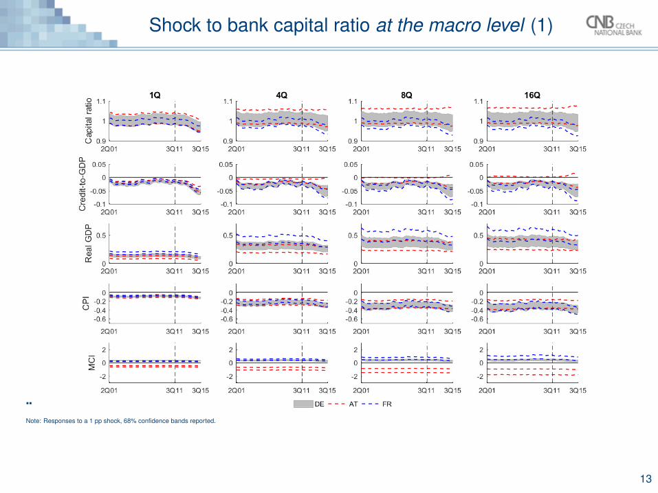
Shock to bank capital ratio at the macro level (1)

Note: Responses to a 1 pp shock, 68% confidence bands reported.

14

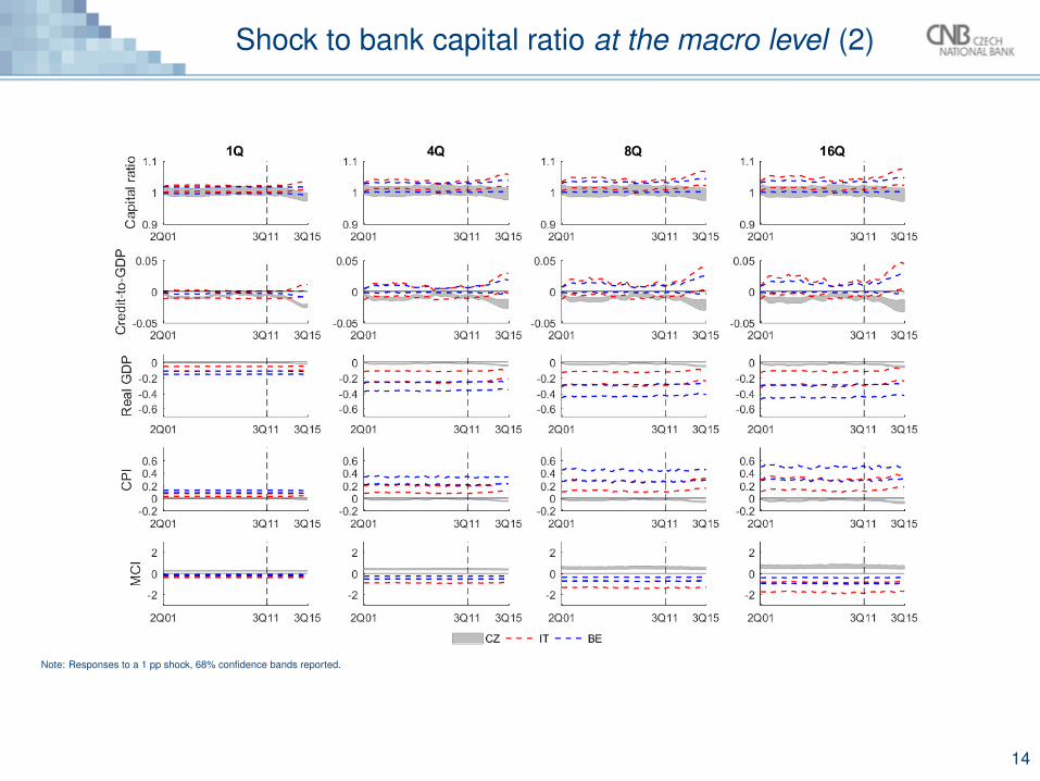
Shock to bank capital ratio at the macro level (2)

• Effect can be divided into two main categories:• resulting in monetary tightening which in turn decreases inflation and

reduces the credit-to-GDP ratio (DE, FR, CZ),• resulting in monetary easing which in turn increases inflation and

pushes up the credit-to-GDP ratio (BE, IT, AT).• Different capitalisation of banking sector in each country may play

a role• Higher capital ratio may increase confidence in under-capitalised

banks, reduce banks’ overall funding costs and help underpin asustained recovery in credit growth and vice versa

Table: Cross-country comparison of mean and median equity-to-assets ratio, BankscopeAT BE CZ DE FR IT

Mean 7.49% 7.18% 10.07% 8.24% 9.18% 8.08%Median 7.29% 6.21% 9.52% 8.13% 8.46% 7.71%

15

Effect of shock to bank capital ratio

Controlling for macroeconomic conditions and bank characteristics, weshould expect• a generally negative correlation between bank capital ratio and its

loan growth,• a positive correlation between bank capital ratio and its loan

growth in case of under-capitalised banks (impact of highercapitalisation on bank confidence which in turn reduces its fundingcost and boosts up the loan growth).

16

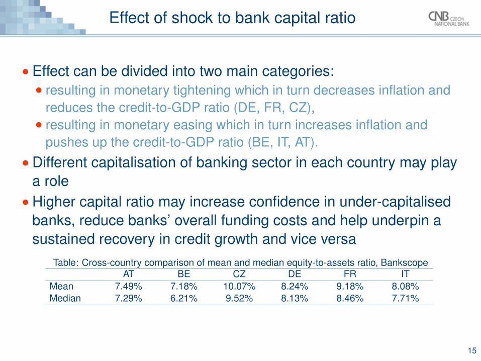
Testable hypotheses

(1) (2) (3) (4) (5)

Dependent variable Loangrowth

Loangrowth

Loangrowth

Loangrowth

Loangrowth

Capital ratio E/A E/RWARegulatory

capitalratio

E/Alower q.

E/Aupper q.

Loan growth (t-1) 0.194* 0.147* 0.119 0.279** -0.184**(0.099) (0.079) (0.0810) (0.111) (0.072)

Short-term rate -26.350* -31.366* -30.703* 1.386* -3.044**(15.044) (16.304) (16.592) (0.747) (1.291)

Yield curve slope 5.225 5.736* 5.214 -0.471 2.321*(3.211) (3.353) (3.324) (1.158) (1.280)

Real GDP growth 4.442** 4.703** 4.374** 0.695 2.018**(2.051) (2.051) (2.154) (0.589) (0.853)

CPI inflation -0.268 -0.224 -0.195 -0.519 1.252(0.398) (0.452) (0.484) (0.559) (1.216)

Capital ratio 2.692 0.512 0.14 4.802** 0.195(2.275) (0.359) (0.207) (2.423) (0.873)

Capital ratio (t-1) -2.386 -0.219 -0.231* -3.473 -0.034(2.141) (0.376) (0.139) (2.295) (0.669)

+ other controls ... ... ... ... ...Observations 971 971 971 253 243Banks 688 688 688 163 175Instruments 37 37 37 51 37

17

Micro-level analysis

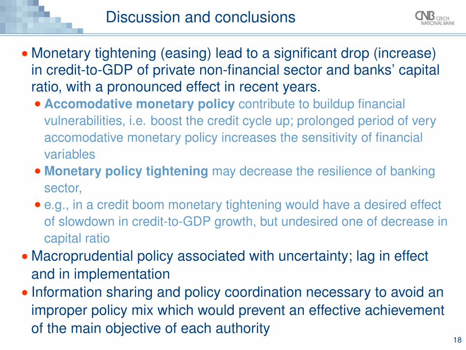
•Monetary tightening (easing) lead to a significant drop (increase)in credit-to-GDP of private non-financial sector and banks’ capitalratio, with a pronounced effect in recent years.• Accomodative monetary policy contribute to buildup financial

vulnerabilities, i.e. boost the credit cycle up; prolonged period of veryaccomodative monetary policy increases the sensitivity of financialvariables• Monetary policy tightening may decrease the resilience of banking

sector,• e.g., in a credit boom monetary tightening would have a desired effect

of slowdown in credit-to-GDP growth, but undesired one of decrease incapital ratio

•Macroprudential policy associated with uncertainty; lag in effectand in implementation• Information sharing and policy coordination necessary to avoid an

improper policy mix which would prevent an effective achievementof the main objective of each authority

18

Discussion and conclusions

THANK YOU FOR YOUR ATTENTION

19

Adrian, T., & Liang, N. 2014. Monetary Policy, Financial Conditions, and Financial Stability. Staff Report 690. Federal ReserveBank of New York.

Blundell, Richard, & Bond, Stephen R. 1998. Initial Conditions and Moment Restrictions in Dynamic Panel Data Models.Journal of Econometrics, 87(1), 115–143.

Borio, C. 2014. Monetary Policy and Financial Stability: What Role in Prevention and Recovery? BIS Working Papers 440.Bank for International Settlements.

Borio, Claudio, & Zhu, Haibin. 2014. Capital Regulation, Risk-taking and Monetary Policy: A Missing Link in the TransmissionMechanism? Journal of Financial Stability, 8(4), 236–51.

Borio, Claudio, Gambacorta, Leonardo, & Hofmann, Boris. 2015. The Influence of Monetary Policy on Bank Profitability. BISWorking Papers 514. Bank for International Settlements.

Canova, F., & Ciccarelli, M. 2009. Estimating Multicountry VAR Model. International Economic Review, 50(3), 929–959.Lowe, Philip, & Borio, Claudio. 2002. Asset Prices, Financial and Monetary Stability: Exploring the Nexus. BIS Working

Papers 114. Bank for International Settlements.Windmeijer, Frank. 2005. A finite sample correction for the variance of linear efficient two-step GMM estimators. Journal of

Econometrics, 126(1), 25–51.

20

References I

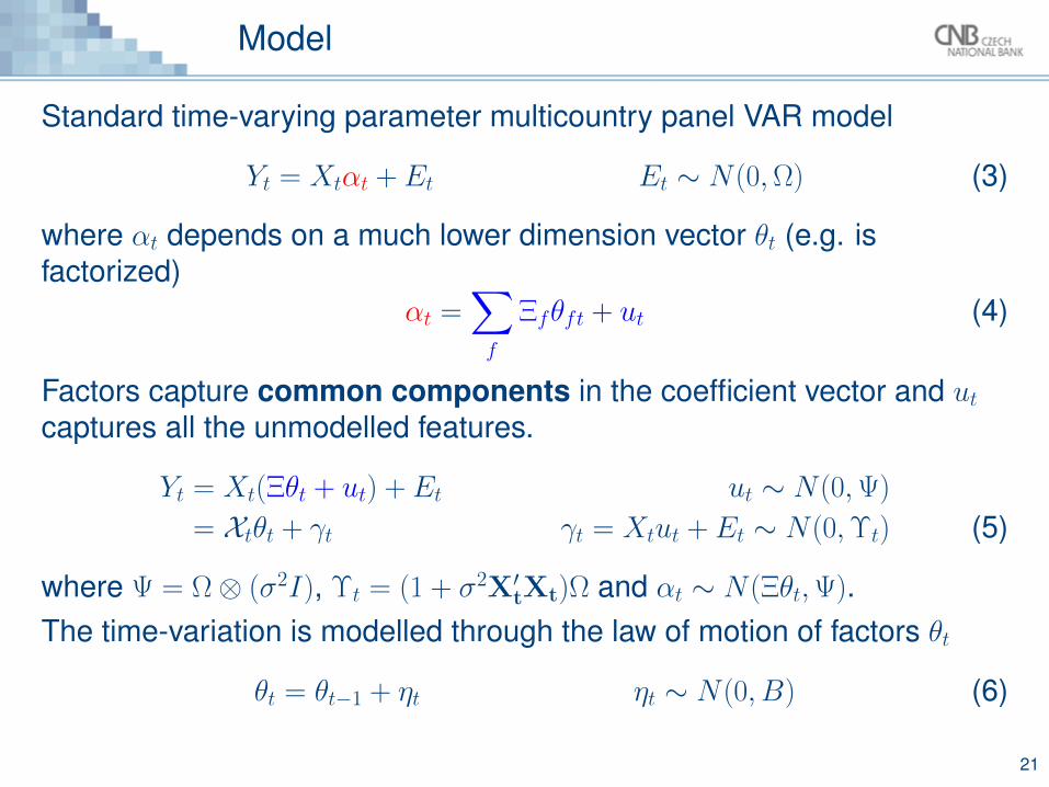
Standard time-varying parameter multicountry panel VAR model

Yt = Xtαt + Et Et ∼ N(0,Ω) (3)

where αt depends on a much lower dimension vector θt (e.g. isfactorized)

αt =∑f

Ξfθft + ut (4)

Factors capture common components in the coefficient vector and utcaptures all the unmodelled features.

Yt = Xt(Ξθt + ut) + Et ut ∼ N(0,Ψ)

= Xtθt + γt γt = Xtut + Et ∼ N(0,Υt) (5)

where Ψ = Ω⊗ (σ2I), Υt = (1 + σ2X′tXt)Ω and αt ∼ N(Ξθt,Ψ).The time-variation is modelled through the law of motion of factors θt

θt = θt−1 + ηt ηt ∼ N(0, B) (6)

21

Model

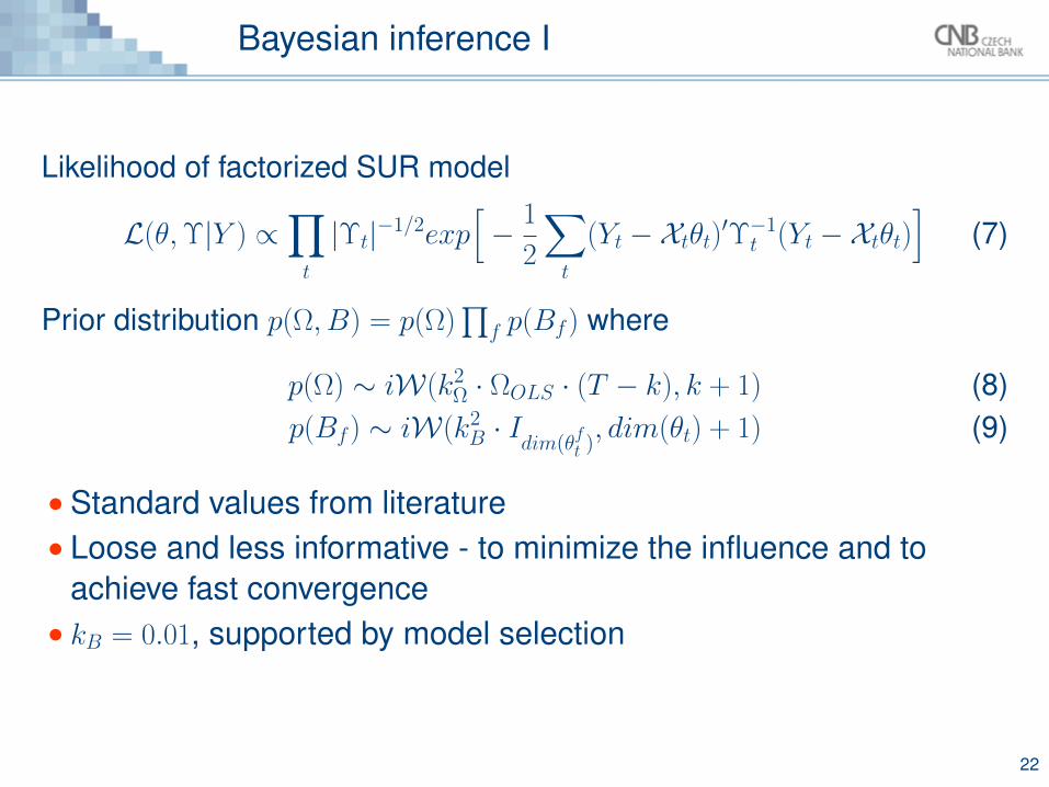
Likelihood of factorized SUR model

L(θ,Υ|Y ) ∝∏t

|Υt|−1/2exp[− 1

2

∑t

(Yt −Xtθt)′Υ−1t (Yt −Xtθt)

](7)

Prior distribution p(Ω, B) = p(Ω)∏

f p(Bf) where

p(Ω) ∼ iW(k2Ω · ΩOLS · (T − k), k + 1) (8)

p(Bf) ∼ iW(k2B · Idim(θ

ft ), dim(θt) + 1) (9)

• Standard values from literature• Loose and less informative - to minimize the influence and to

achieve fast convergence• kB = 0.01, supported by model selection

22

Bayesian inference I

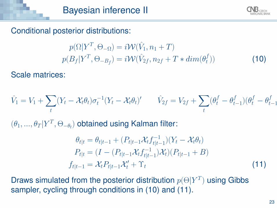
Conditional posterior distributions:

p(Ω|Y T ,Θ−Ω) = iW(V1, n1 + T )

p(Bf |Y T ,Θ−Bf ) = iW(V2f , n2f + T ∗ dim(θft )) (10)

Scale matrices:

V1 = V1 +∑t

(Yt −Xtθt)σ−1t (Yt −Xtθt)′ V2f = V2f +

∑t

(θft − θft−1)(θft − θ

ft−1)′

(θ1, ..., θT |Y T ,Θ−θt) obtained using Kalman filter:

θt|t = θt|t−1 + (Pt|t−1Xtf−1t|t−1)(Yt −Xtθt)

Pt|t = (I − (Pt|t−1Xtf−1t|t−1)Xt)(Pt|t−1 + B)

ft|t−1 = XtPt|t−1X ′t + Υt (11)

Draws simulated from the posterior distribution p(Θ|Y T ) using Gibbssampler, cycling through conditions in (10) and (11).

23

Bayesian inference II

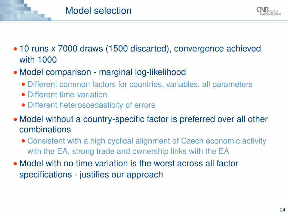
• 10 runs x 7000 draws (1500 discarted), convergence achievedwith 1000•Model comparison - marginal log-likelihood• Different common factors for countries, variables, all parameters• Different time-variation• Different heteroscedasticity of errors

•Model without a country-specific factor is preferred over all othercombinations• Consistent with a high cyclical alignment of Czech economic activity

with the EA, strong trade and ownership links with the EA•Model with no time variation is the worst across all factor

specifications - justifies our approach

24

Model selection