Monetary and Fiscal Policies: Sustainable Fiscal · PDF fileMonetary and Fiscal Policies:...

Monetary and Fiscal Policies:Sustainable Fiscal Policies

Behzad Diba

Georgetown University

May 2013

(Institute) Monetary and Fiscal Policies: Sustainable Fiscal Policies May 2013 1 / 13

What is Sustainable?

Empirical assessments of the fiscal stance are complicated by the factthat we don’t have a precise definition of fiscal sustainability

For example, the debt-to-GDP ratio may grow in a particular sample,but this does not mean it will continue to grow in the future

Or, the ratio may be stable, while (say) the effects of an agingpopulation and unfunded fiscal obligations pose a future challenge

Much of the existing empirical research has focused on developingeconometric tests of whether or not the government PVBC issatisfied, given the trends we can detect from data

A more useful approach may provide measures of the fiscal outlookwithout attempting a formal test for sustainability


"Testing" for the PVBC?

In retrospect, earlier attempts to develop econometric tests of thePVBC (based on stationarity and co-integration tests) don’t seemvery informative

1 The tests amount to asking if the transversality condition of lenderswill be satisfied as time tends to infinity; this is not a question in theusual realm of statistical inference

2 We now understand (following the FTPL) that the "PVBC" is anequilibrium condition; there is no formal theoretical motivation for an"alternative hypothesis" that the PVBC does not hold

3 It is not clear what satisfying the PVBC has to do with fiscalsustainability, as the following example illustrates


An Example

As discussed in CCD (2010), the government’s PVBC is derived usingthe transversality condition (TC) of households (lenders)

In a benchmark model with logarithmic utility, the TC implies

limn→+∞

βnEt

{Lt+n

Pt+nCt+n

}= 0 ,

stating that the ratio of nominal public debt to nominal consumption,discounted at the lenders’rate of time preference, is expected toconverge to zero; standard calibrations set β = 0.99 per quarter

the ratio of debt to aggregate consumption can grow exponentially (atany rate less than 4% per annum) without violating the PVBCbut most of us would probably consider such a fiscal policy, making thedebt-to-GDP ratio grow forever, unsustainable

In the model (with simplifying features like infinite horizons, alump-sum tax, etc.), an equilibrium can involve an ever growingdebt-to-GDP ratio, but this implication is not robust to changes inthe model (like considering overlapping generations of households)


An Example

As discussed in CCD (2010), the government’s PVBC is derived usingthe transversality condition (TC) of households (lenders)In a benchmark model with logarithmic utility, the TC implies

limn→+∞

βnEt

{Lt+n

Pt+nCt+n

}= 0 ,





An Example


limn→+∞

βnEt

{Lt+n

Pt+nCt+n

}= 0 ,


the ratio of debt to aggregate consumption can grow exponentially (atany rate less than 4% per annum) without violating the PVBC

but most of us would probably consider such a fiscal policy, making thedebt-to-GDP ratio grow forever, unsustainable



An Example


limn→+∞

βnEt

{Lt+n

Pt+nCt+n

}= 0 ,





Dynamics of Debt/GDP

Let bt denote the real value of government bonds outstanding at timet, and let rt denote the ex-post real return on bonds, debt dynamicsare governed by

bt = (1+ rt )bt−1 + Gt − Tt ,

where Tt is tax revenues inclusive of seigniorage

The evolution of the debt-to-GDP ratio is governed by

btYt= (1+ ρt )

bt−1Yt−1

+Gt − TtYt

, (1)

with

1+ ρt = (1+ rt )(Yt−1Yt

)


Steady-state Equilibrium

Standard calibrations used for policy analysis assume, and standardasset pricing models imply, that the real return on debt exceeds thereal growth rate in the long run (on the balanced growth path)

for example, the "benchmark scenarios" of IMF (2010) assume the realinterest rate exceeds the real growth rate by one percentage point perannumand, as a theoretical benchmark, the CCAPM with logarithmic utilityimplies that the steady-state real rate equals the subjective rate of timepreference plus the growth rate of per-capita real consumption

With ρ > 0, the steady-state version of (1) is

ρ

(bY

)=T − GY

,

which implies that a government with positive debt must run aprimary surplus (inclusive of seigniorage) that services the debt andkeeps the debt-to-GDP ratio constant




for example, the "benchmark scenarios" of IMF (2010) assume the realinterest rate exceeds the real growth rate by one percentage point perannum

and, as a theoretical benchmark, the CCAPM with logarithmic utilityimplies that the steady-state real rate equals the subjective rate of timepreference plus the growth rate of per-capita real consumption


ρ

(bY

)=T − GY

,





for example, the "benchmark scenarios" of IMF (2010) assume the realinterest rate exceeds the real growth rate by one percentage point perannumand, as a theoretical benchmark, the CCAPM with logarithmic utilityimplies that the steady-state real rate equals the subjective rate of timepreference plus the growth rate of per-capita real consumption


ρ

(bY

)=T − GY

,



Log-linear Approximation

We can log-linearize (1) near a steady state (with ρt = ρ, etc.) to get

log(btYt

)= Φ+ φg log

(GtYt

)− φτ log

(TtYt

)+ φρ log (1+ ρt )

+(1+ ρ) log(bt−1Yt−1

)with coeffi cients Φ, φg > 0, φτ > 0, and φρ > 0 that depend only onthe point of approximation

Iterating on this linear equation, Polito and Wickens (2012) analyzethe change in the debt-to-GDP ratio, over finite horizons


Growth in Debt/GDP

The log-linear relationship links the growth in the debt-to GDP ratioto components reflecting revenues, expenditures, and the discountrate (ρt)

It is instructive to plot these components and interpret historicalchanges in the debt-to-GDP ratio, as Polito and Wickens (2012) do

Polito and Wickens (2012) also estimate a VAR involving the fiscalvariables, inflation, short-term and long-term interest rates, and theGDP gap

They use the VAR forecasts to predict / project changes in thedebt-to-GDP ratio

the details serve to illustrate the econometric approach but are not ofdirect interest to us, because the forecast horizons are shortwe may speculate about some correlations in the data


Figure 1: The United States: data plot

1970 1975 1980 1985 1990 1995 2000 2005 201020

30

40

50

60

70

80

90

100A: DebtGDP

1970 1975 1980 1985 1990 1995 2000 2005 201025

30

35

40

45B: RevenueGDP (REV) and SpendingGDP (SPE)

REV

SPE

1970 1975 1980 1985 1990 1995 2000 2005 201010

5

0

5

10C: Inflation and output gap

INF

GAP

1970 1975 1980 1985 1990 1995 2000 2005 201010

5

0

5

10

15

20

D: Interest rates: Longterm (IRL), Shortterm (IRS) andimplicit rate on government debtGDP ratio ( ρ)

IRL

IRS

ρ

Figure 2: The United Kingdom: data plot

1970 1975 1980 1985 1990 1995 2000 2005 201020

30

40

50

60

70

80

90

100A: DebtGDP

1970 1975 1980 1985 1990 1995 2000 2005 201035

40

45

50


REV

SPE

1970 1975 1980 1985 1990 1995 2000 2005 201010

5

0

5

10

15

20

25


INF

GAP

1970 1975 1980 1985 1990 1995 2000 2005 201020

15

10

5

0

5

10

15

20


IRLIRS

ρ

19

Figure 3: Germany: data plot

1970 1975 1980 1985 1990 1995 2000 2005 201010

20

30

40

50

60

70

80

90

100A: DebtGDP

1970 1975 1980 1985 1990 1995 2000 2005 201035

40

45

50


REV

SPE

1970 1975 1980 1985 1990 1995 2000 2005 20105

0

5


INF

GAP

1970 1975 1980 1985 1990 1995 2000 2005 201020

15

10

5

0

5

10

15

20


IRL

IRS

ρ

Figure 4: Greece: data plot

1970 1975 1980 1985 1990 1995 2000 2005 20100

20

40

60

80

100

120

140A: DebtGDP

1970 1975 1980 1985 1990 1995 2000 2005 201020

25

30

35

40

45

50


REV

SPE

1970 1975 1980 1985 1990 1995 2000 2005 201020

10

0

10

20


INF

GAP

1970 1975 1980 1985 1990 1995 2000 2005 201020

15

10

5

0

5

10

15

20

25


IRL

IRS

ρ

20

Figure 1: The United States: data plot

1970 1975 1980 1985 1990 1995 2000 2005 201020

30

40

50

60

70

80

90

100A: DebtGDP

1970 1975 1980 1985 1990 1995 2000 2005 201025

30

35

40


REV

SPE

1970 1975 1980 1985 1990 1995 2000 2005 201010

5

0

5


INF

GAP

1970 1975 1980 1985 1990 1995 2000 2005 201010

5

0

5

10

15

20


IRL

IRS

ρ

Figure 2: The United Kingdom: data plot

1970 1975 1980 1985 1990 1995 2000 2005 201020

30

40

50

60

70

80

90

100A: DebtGDP

1970 1975 1980 1985 1990 1995 2000 2005 201035

40

45

50


REV

SPE

1970 1975 1980 1985 1990 1995 2000 2005 201010

5

0

5

10

15

20

25


INF

GAP

1970 1975 1980 1985 1990 1995 2000 2005 201020

15

10

5

0

5

10

15

20


IRLIRS

ρ

19

Figure 3: Germany: data plot

1970 1975 1980 1985 1990 1995 2000 2005 201010

20

30

40

50

60

70

80

90

100A: DebtGDP

1970 1975 1980 1985 1990 1995 2000 2005 201035

40

45

50


REV

SPE

1970 1975 1980 1985 1990 1995 2000 2005 20105

0

5


INF

GAP

1970 1975 1980 1985 1990 1995 2000 2005 201020

15

10

5

0

5

10

15

20


IRL

IRS

ρ

Figure 4: Greece: data plot

1970 1975 1980 1985 1990 1995 2000 2005 20100

20

40

60

80

100

120

140A: DebtGDP

1970 1975 1980 1985 1990 1995 2000 2005 201020

25

30

35

40

45

50


REV

SPE

1970 1975 1980 1985 1990 1995 2000 2005 201020

10

0

10

20


INF

GAP

1970 1975 1980 1985 1990 1995 2000 2005 201020

15

10

5

0

5

10

15

20

25


IRL

IRS

ρ

20

Growth in Debt/GDP







Growth in Debt/GDP





the details serve to illustrate the econometric approach but are not ofdirect interest to us, because the forecast horizons are short

we may speculate about some correlations in the data


Growth in Debt/GDP







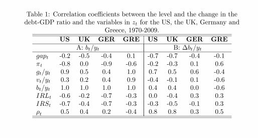
change in the debt-GDP ratio is stronger.

Table 1: Correlation coe¢ cients between the level and the change in thedebt-GDP ratio and the variables in zt for the US, the UK, Germany and

Greece, 1970-2009.US UK GER GRE US UK GER GRE

A: bt=yt B: �bt=ytgapt -0.2 -0.5 -0.4 0.1 -0.7 -0.7 -0.4 -0.1�t -0.8 0.0 -0.9 -0.6 -0.2 -0.3 0.1 0.6gt=yt 0.9 0.5 0.4 1.0 0.7 0.5 0.6 -0.4vt=yt 0.3 0.2 0.4 0.9 -0.4 -0.1 0.1 -0.6bt=yt 1.0 1.0 1.0 1.0 0.4 0.4 0.0 -0.6IRLt -0.6 -0.2 -0.7 -0.3 0.0 -0.4 0.3 0.3IRSt -0.7 -0.4 -0.7 -0.3 -0.3 -0.5 -0.1 0.3�t 0.5 0.4 0.2 -0.4 0.8 0.8 0.3 0.5

5.1.2 Econometric tests of �scal sustainability

For the purposes of comparison, and before computing the index, we carry outsome of the econometric tests of �scal sustainability discussed earlier. Table2 reports the Augmented Dickey-Fuller (ADF) and Phillips-Perron (PP) teststatistics for the ratios of debt and the de�cit to GDP under various assumptionsabout the discount rate.The Hamilton and Flavin test described in equation (13) is based on the

stationarity of the undiscounted processes dtyt andbtyt: if they are not stationary

then the �scal stance is said to be unsustainable. They argue - and this wasshown earlier - that, under the assumption of a positive constant interest rate,the discounted sum of future de�cits is stationary if the undiscounted process dtytis stationary. Panel A gives the ADF and PP tests statistics for the undiscountedseries bt

ytand dt

yt. The hypothesis of a unit root cannot be rejected for the debt-

GDP ratios at any conventional signi�cance level, but the outcomes for theundiscounted processes dt

ytdepend upon the choice of unit root test and on the

signi�cance level. Although the results for the debt-GDP ratio suggest thatthe �scal stance is not sustainable, those for the de�cit-GDP ratio create someambiguity.The test is repeated in Panel B using discounted series for bt=yt and dt=yt

where the discount rate is a constant equal to the sample average of �t. Interms of the earlier discussion, these are tests of the transversality condition andthe PVBC, equations (8) and (9) respectively. The results are now even moreambiguous. Using the ADF test the null hypothesis of a unit root is not rejectedfor any country but using the PP test the outcome is marginal. dt=yt appearsto be non-stationary except for Germany. In Panel C the tests are repeatedagain only this time under the assumption of a time-varying discount rate. This

21

Limitations

The VAR approach cannot forecast fiscal stress caused by factors thatare not reflected in past data

as illustrated by our earlier discussion of aging populations andunfunded liabilitiesexpert projection— like the CBO projections, and their extensions,discussed in Auerbach (2011)—may be used in conjunction with themore objective statistical approach

Calculating a reliable measure of the relevant discount rate ρt iscomplicated by data limitations

Bohn’s (2008) analysis of historical US data motivates more work onmeasuring ρHall and Sargent (2010) present a measurement methodology; they alsocompare their measure of ρt to simple measures that are commonlyused and conclude that the simple measures can be quite misleading


Limitations


as illustrated by our earlier discussion of aging populations andunfunded liabilities

expert projection— like the CBO projections, and their extensions,discussed in Auerbach (2011)—may be used in conjunction with themore objective statistical approach




Limitations






Limitations




Bohn’s (2008) analysis of historical US data motivates more work onmeasuring ρ

Hall and Sargent (2010) present a measurement methodology; they alsocompare their measure of ρt to simple measures that are commonlyused and conclude that the simple measures can be quite misleading


Limitations






Expert Projections

Auerbach (2011) illustrates the approach used in his work withWilliam Gale and summarizes some results

the fiscal gap over a horizon from the current date t to a terminal dateT measures the required increase in the primary surplus (relative tocurrent projections) that would be needed to maintain debt/GDP at itscurrent valueAuerbach and Gale (2011) estimated a fiscal gap in the 3 to 6 percentrange through 2060 for the US federal-governmentthe estimates assumed an interest rate exceeding the GDP growth rateby one percentage pointAuerbach and Gale (2011) noted that the fiscal gaps can besignificantly larger (as large as 10% of GDP) if interest rates riserelative to GDP growth or the horizon is extended beyond 2060

Auerbach (2011) reports fiscal gaps for other advanced economies


Expert Projections


the fiscal gap over a horizon from the current date t to a terminal dateT measures the required increase in the primary surplus (relative tocurrent projections) that would be needed to maintain debt/GDP at itscurrent value

Auerbach and Gale (2011) estimated a fiscal gap in the 3 to 6 percentrange through 2060 for the US federal-governmentthe estimates assumed an interest rate exceeding the GDP growth rateby one percentage pointAuerbach and Gale (2011) noted that the fiscal gaps can besignificantly larger (as large as 10% of GDP) if interest rates riserelative to GDP growth or the horizon is extended beyond 2060



Calculating Fiscal Gaps

The evolution of debt implies

BT(1 + r)T−t

= Bt +

T∑s=t+1

Ds(1 + r)s−t

where B is the stock of government bonds, D is the primary deficit, and r isthe interest rate (assumed to be constant for simplicity).The fiscal gap ∆ is the annual deficit reduction that keeps the debt-to-GDP

ratio at the terminal date T equal to the current value at t:

BTYT

=BtYt

So, ∆ satisfies

BtYTYt(1 + r)T−t

= Bt +

T∑s=t+1

Ds −∆Ys(1 + r)s−t

which implies

∆ =Bt −Bt (YT /Yt) (1 + r)t−T +

∑Ts=t+1(1 + r)t−sDs∑T

s=t+1(1 + r)t−sYs

1

Expert Projections


the fiscal gap over a horizon from the current date t to a terminal dateT measures the required increase in the primary surplus (relative tocurrent projections) that would be needed to maintain debt/GDP at itscurrent valueAuerbach and Gale (2011) estimated a fiscal gap in the 3 to 6 percentrange through 2060 for the US federal-government

the estimates assumed an interest rate exceeding the GDP growth rateby one percentage pointAuerbach and Gale (2011) noted that the fiscal gaps can besignificantly larger (as large as 10% of GDP) if interest rates riserelative to GDP growth or the horizon is extended beyond 2060



Expert Projections


the fiscal gap over a horizon from the current date t to a terminal dateT measures the required increase in the primary surplus (relative tocurrent projections) that would be needed to maintain debt/GDP at itscurrent valueAuerbach and Gale (2011) estimated a fiscal gap in the 3 to 6 percentrange through 2060 for the US federal-governmentthe estimates assumed an interest rate exceeding the GDP growth rateby one percentage point

Auerbach and Gale (2011) noted that the fiscal gaps can besignificantly larger (as large as 10% of GDP) if interest rates riserelative to GDP growth or the horizon is extended beyond 2060



Expert Projections


the fiscal gap over a horizon from the current date t to a terminal dateT measures the required increase in the primary surplus (relative tocurrent projections) that would be needed to maintain debt/GDP at itscurrent valueAuerbach and Gale (2011) estimated a fiscal gap in the 3 to 6 percentrange through 2060 for the US federal-governmentthe estimates assumed an interest rate exceeding the GDP growth rateby one percentage pointAuerbach and Gale (2011) noted that the fiscal gaps can besignificantly larger (as large as 10% of GDP) if interest rates riserelative to GDP growth or the horizon is extended beyond 2060



Fiscal Gaps

The fiscal gap calculations are versatile for quantifying theimplications of alternative scenarios and assumptions

Auerbach (2011) considers scenarios with

no initial debtnet debt going to a 45% target recommended in IMF (2010)higher differentials between interest rates and GDP growth

Notably, projected growth of health and pension expenditures (relativeto GDP) contributes more than initial debt positions to fiscal gaps

The Debt-to-GDP ratio may not be a very reliable measure of fiscalstress


Fiscal Gaps



no initial debt

net debt going to a 45% target recommended in IMF (2010)higher differentials between interest rates and GDP growth




Fiscal Gaps



no initial debtnet debt going to a 45% target recommended in IMF (2010)

higher differentials between interest rates and GDP growth




Fiscal Gaps



no initial debtnet debt going to a 45% target recommended in IMF (2010)higher differentials between interest rates and GDP growth




Historical US Data

Bohn (2008) analyzed US data over 1792-2003

he introduced an approach to testing for sustainability [alsosummarized in Polito and Wickens (2012)] based on a regression ofsurplus/GDP on debt/GDPhe concluded that U.S. fiscal policy was sustainable, based on apositive response of surplus/GDP to debt/GDP and evidence of meanreversion in debt/GDPalthough subsequent data cast doubt on this conclusion, the basicmethodology remains of interest

An important contribution of Bohn (2008) was in documenting therole of economic growth and the low return on short-term Treasurydebt in stabilizing debt/GDP

the reason debt/GDP did not grow was that the growth attributable toprimary deficits and interest payments was offset by "the growthdividend" arising from erosion of debt/GDPthe interest cost of debt was on average below the growth rate of GDP


Historical US Data


he introduced an approach to testing for sustainability [alsosummarized in Polito and Wickens (2012)] based on a regression ofsurplus/GDP on debt/GDP

he concluded that U.S. fiscal policy was sustainable, based on apositive response of surplus/GDP to debt/GDP and evidence of meanreversion in debt/GDPalthough subsequent data cast doubt on this conclusion, the basicmethodology remains of interest




Historical US Data


he introduced an approach to testing for sustainability [alsosummarized in Polito and Wickens (2012)] based on a regression ofsurplus/GDP on debt/GDPhe concluded that U.S. fiscal policy was sustainable, based on apositive response of surplus/GDP to debt/GDP and evidence of meanreversion in debt/GDP

although subsequent data cast doubt on this conclusion, the basicmethodology remains of interest




Figure 1: The U.S. Public Debt, Nominal (line) and real (dotted), 1900-2003

0

500

1000

1500

2000

2500

3000

3500

4000

4500

1900 1920 1940 1960 1980 2000

Figure 2: The U.S. Public Debt in Percent of GDP 1791-2003

0%

20%

40%

60%

80%

100%

120%

1790 1820 1850 1880 1910 1940 1970 2000

Historical US Data






Historical US Data




the reason debt/GDP did not grow was that the growth attributable toprimary deficits and interest payments was offset by "the growthdividend" arising from erosion of debt/GDP

the interest cost of debt was on average below the growth rate of GDP


Table 1: Deficits versus Changes in the Debt-GDP Ratio Period:

From

To

With

interest

Deficit

Primary

Deficit

Interest

Charge

Nominal

Growth

Effect

Real

Growth

Effect

Inflation

Effect

Change in

Debt/GDP

(1) (2) (3) (4) (5) (6) (7)

1792 2003 1.2% 0.3% 0.9% 1.3% 0.8% 0.5% 0.0%

1792 1868 0.4% -0.1% 0.5% 0.6% 0.5% 0.1% -0.1%

1869 2003 1.7% 0.5% 1.2% 1.7% 1.0% 0.7% 0.0%

1792 1914 0.1% -0.4% 0.5% 0.5% 0.5% 0.0% -0.3%

1915 2003 2.8% 1.2% 1.6% 2.4% 1.2% 1.2% 0.4%

Table 2: Interest Rates on Public Debt versus Growth Rates

Period:

From

To

Interest

Rate *

Nominal

Growth

Real

Growth

Inflation Interest-

Growth

(1) (2) (3) (4) (5)

1792 2003 4.5% 5.2% 3.8% 1.4% -0.6%

1792 1868 4.8% 4.9% 4.2% 0.6% -0.1%

1869 2003 4.4% 5.3% 3.5% 1.8% -1.0%

1792 1914 4.6% 4.3% 4.1% 0.2% 0.4%

1915 2003 4.4% 6.4% 3.4% 3.1% -2.1%

Notes: * The interest rate on public debt is computed as the ratio of interest payments over the average of outstanding debt at the start and the end of each year.

Historical US Data






Table 1: Deficits versus Changes in the Debt-GDP Ratio Period:

From

To

With

interest

Deficit

Primary

Deficit

Interest

Charge

Nominal

Growth

Effect

Real

Growth

Effect

Inflation

Effect

Change in

Debt/GDP

(1) (2) (3) (4) (5) (6) (7)

1792 2003 1.2% 0.3% 0.9% 1.3% 0.8% 0.5% 0.0%

1792 1868 0.4% -0.1% 0.5% 0.6% 0.5% 0.1% -0.1%

1869 2003 1.7% 0.5% 1.2% 1.7% 1.0% 0.7% 0.0%

1792 1914 0.1% -0.4% 0.5% 0.5% 0.5% 0.0% -0.3%

1915 2003 2.8% 1.2% 1.6% 2.4% 1.2% 1.2% 0.4%

Table 2: Interest Rates on Public Debt versus Growth Rates

Period:

From

To

Interest

Rate *

Nominal

Growth

Real

Growth

Inflation Interest-

Growth

(1) (2) (3) (4) (5)

1792 2003 4.5% 5.2% 3.8% 1.4% -0.6%

1792 1868 4.8% 4.9% 4.2% 0.6% -0.1%

1869 2003 4.4% 5.3% 3.5% 1.8% -1.0%

1792 1914 4.6% 4.3% 4.1% 0.2% 0.4%

1915 2003 4.4% 6.4% 3.4% 3.1% -2.1%

Notes: * The interest rate on public debt is computed as the ratio of interest payments over the average of outstanding debt at the start and the end of each year.

Post WWII US Data

Hall and Sargent (2010) develop a measurement framework forcalculating returns on US government bonds with different maturities

They find (like Bohn) that economic growth played the mostimportant role in stabilizing debt/GDP

They also document interesting variations in returns across debtmaturities and analyze the sources of change in the debt-to-GDPratio during various episodes

Recent commentary (by Bohn and others) questions the wisdom ofcontinuing US reliance on short-term "safe" debt to finance budgetdeficits


Monetary and Fiscal Policies: Sustainable Fiscal · PDF fileMonetary and Fiscal Policies:...

Documents

Transcript of Monetary and Fiscal Policies: Sustainable Fiscal · PDF fileMonetary and Fiscal Policies:...