Monash Universityusers.monash.edu.au/~gholamrh/lab/hon2015-andi-thesis.pdf · 1 Monash University...

1

Monash University

Bayesian Changepoint

Detection in Textual Data

Streams

This thesis is presented in partial fulfilment of the requirements for the degree

of Bachelor of Computer Science (Honours) at Monash University

By

Andisheh Partovi

Supervisors

Gholamreza Haffari – Ingrid Zukerman

Year

2015

2

Abstract

Text Mining is the process of extracting useful information from textual data

sources and has numerous applications in different fields. Statistical

changepoint detection techniques can provide a new tool for temporal analysis

of texts that can reveal interesting trends in the data over time. In this research,

a generic real-time changepoint detection algorithm has been adapted to work

with streams of textual data for two distinct tasks: detecting changes in the topic

and detecting changes in the author. The performance of the system is

evaluated on a synthetic corpus and two real corpora: the State of the Union

addresses and Twitter messages.

3

Declaration

I declare that this thesis is my own work and has not been submitted in any

form for another degree or diploma at any university or other institute of tertiary

education. Information derived from the work of others has been

acknowledged.

Signed by

Andisheh Partovi

01/07/2015

4

Acknowledgements

Foremost I would like to thank my supervisors Reza Haffari and Ingrid

Zukerman for their support and guidance throughout this research. I want to

especially thank Reza for helping with the design of the likelihood model and

Ingrid for reviewing this thesis.

I’d also like to thank my fiancé, Zahra, whose patience, endless love, and

support made this research not only possible but enjoyable as well.

Thank you very much everyone!

Andisheh Partovi

5

Contents

Abstract ............................................................................................................ 2

1 Introduction ............................................................................................... 7

2 Literature Review ...................................................................................... 9

Sentiment Analysis on Twitter ............................................................. 9

2.1.1 Twitter Anatomy ........................................................................... 9

2.1.2 Previous Work on Text Mining ................................................... 10

The Changepoint Detection Problem ................................................ 12

2.2.1 The Existing Methods ................................................................. 13

Changepoint Detection on Twitter ..................................................... 17

Authorship Attribution ....................................................................... 19

3 Methods .................................................................................................. 21

Overview of the Method .................................................................... 21

The Probability Calculations ............................................................. 23

3.2.1 Prior Probability of Change ........................................................ 24

3.2.2 The Likelihood ............................................................................ 24

3.2.3 Implementation Issues ............................................................... 27

The Recursive Algorithm................................................................... 29

4 Experiments ............................................................................................ 30

Data .................................................................................................. 30

4.1.1 News Articles Corpus ................................................................. 30

4.1.2 State of the Union Addresses ..................................................... 30

4.1.3 Tweets ........................................................................................ 31

Features............................................................................................ 32

4.2.1 Topic Change Task .................................................................... 32

4.2.2 Authorship Change Task ............................................................ 33

Preprocessing ................................................................................... 35

Feature Selection .............................................................................. 37

Evaluation Methods .......................................................................... 38


6


Optimisation Methods ....................................................................... 39

5 Results and Analysis .............................................................................. 41

The News Corpus ............................................................................. 41

The State of the Union (SOU) Corpus .............................................. 44



The Hashtag Corpus ......................................................................... 50

Sensitivity Analysis over the Prior Probability ................................... 52

6 Conclusion and Future Work .................................................................. 54

Conclusion ........................................................................................ 54

Towards an Online Setting ................................................................ 55

Future Work ...................................................................................... 56

7 References ............................................................................................. 58

8 List of Figures ......................................................................................... 67

9 List of Tables .......................................................................................... 69

10 Appendix I – Similarity Measures ......................................................... 70

11 Appendix II – Clustering Results .......................................................... 71

7

1 Introduction

Text Mining, or Text Data Mining, is the process of extracting useful information

from textual data sources through identification and exploration of interesting

patterns (Feldman and Sanger, 2007). Since its conception, text mining has

found application in numerous areas from biomedical studies to linguistics and

social sciences.

As web social media, blogging, and online forums can provide vast amounts of

user generated content that can reflect the thoughts and opinions of the users,

their topics of interest, and much more information about the society as a whole,

it is an invaluable source for text mining applications, and hence has been

studied extensively in recent years.

Text mining on social media is not restricted to Twitter. Thelwall and Prabowo

(2007) as well as Bansal and Koudas (2007) worked on online blogs, Kramer

(2010) analysed Facebook status updates to estimate national happiness, and

Kennedy and Inkpen (2006) as well as Pang et al. (2002) worked on classifying

online movie reviews. However, since its launch in 2006, Twitter has attracted

more and more researchers.

As of June 2015, people post more than 500 million Twitter messages (called

tweets) every day (About.twitter.com, 2015), yielding a noisy but sometimes

informative corpus of 140-character messages that reflects their daily activities

and thoughts as well as current events in an unprecedented manner (Ritter et

al., 2011).

Text mining on Twitter has been carried out to extract a variety of different

information. In one study, Bollen et al. (2009) analysed the six dimensions of

emotion in Twitter, showing that these typically reflect significant offline events.

In another study, Bollen et al. (2011) correlated Twitter mood to the changes in

the stock market. Jansen et al. (2009) used tweets to automatically extract

customer opinions about products or brands; Lampos and Cristianini (2010),

Lampos et al. (2010), Paul and Dredze (2011), and Collier and Doan (2011)

used tweets to track infectious diseases; Sakaki et al. (2010) used tweets to

detect earthquakes; and Lampos et al. (2013) used tweets to predict election

winners.

One aspect of text mining is the temporal analysis of the documents, an aspect

that is the focus of a few studies (see Literature Review). If a stream of text (for

instance tweets) is analysed over time, interesting trends such as changes in

topics of interest, meanings of words, or sentiments over time can be revealed.

8

Timely detection of changes in the topic trends or simply the use of language

on Social Media can lead to early discovery of threads to public safety such as

epidemic outbreaks or disasters such as earthquakes. To be able to achieve

this, the change detection must be efficient and capable of processing the data

in real-time as they become available. In this research, we attempt a real-time

solution that does not require the topics or their multiplicity to be known in

advanced.

One of the oldest statistical tools that has been utilised in many problem

domains (see Section 2.2) and can be employed in text mining is changepoint

detection. In this research, a generic Bayesian online change detection

algorithm is adapted to textual data in order to reveal interesting trends in

streams of textual data, especially Twitter messages, over time.

One of the major advantages of the chosen change detection algorithm, is its

versatility that it can be applied to different tasks. These tasks are distinguished

by the kind of change they attempt to detect. To demonstrate this, we undertook

two distinct text mining tasks: detecting changes in the documents’ topic over

time and detecting changes in the documents’ author over time. The first task

is akin to the unsupervised topic segmentation and the second one to

unsupervised authorship attribution.

The rest of this thesis is organised into 6 chapters. First, we present a review

of the existing studies in this field (Literature Review). Then a detailed

explanation of the chosen method (Method) is followed by the experiments we

prepared including the preprocessing and evaluation methods (Experiments).

Next is the results of these experiments along with an analysis of the system

performance (Results and Analysis) before finishing with the conclusion and

proposing ideas for future work (Conclusion and Future Work).

9

2 Literature Review

In this literature review, we will provide a brief description of Twitter, its unique

features, and some of the previous sentiment analysis research on it (Section

2.1); followed by introducing the changepoint detection problem, its

applications, and an analysis of some of the existing methods (Section 2.2);

and reviewing the few existing studies on applying changepoint detection

techniques to Twitter (Section 2.3). We also provide a very brief overview of the

authorship attribution task and how it was used on social media data (2.4).

Sentiment Analysis on Twitter

2.1.1 Twitter Anatomy

Twitter is an online social networking service that enables users to send and

read short 140-character messages. Twitter is mainly used by the public to

share information and to describe minor daily activities (Java et al., 2007).

Although it can also be used for information dissemination, for example, by

government organizations (Wigand, 2010) or private companies. About 80% of

Twitter users update followers on what they are currently doing, while the

remainder centre on information (Naaman et al., 2010).

Tweets are short because of the 140-character limit (117 if they contain a URL)

and therefore have undesirable qualities such as extensive presence of chat

acronyms (such as FTW for "for the win" or OMG for "oh my God") in addition

to qualities common to most online media content such as use of colloquial

terms, emoticons (like ) and emoji1, spelling errors, and alternative spellings

to emphasise a sentiment (such as “reallyyyyy” for “really”).

Because of these features, the performance of standard Natural Language

Processing (NLP) tools can be severely degraded on tweets (Ritter et al., 2011).

When analysing these data, one approach is to take them as they are, without

any modifications. Conversely, the mentioned properties can be eliminated

through normalisation techniques such as designing specialised dictionaries for

emoticons and acronyms and substituting regular expressions resembling a

word with that word. Additionally, standard natural language preprocessing

techniques such as decapitalisation and stop word removal might be

necessary.

1 Emoji are much like emoticons, but with a wider range as they are not restricted to ASCII

characters.

Pre-

processing

What is

Twitter?

10

Another preprocessing step that might be necessary for twitter is removing

tweets with a URL, which are most likely spam (Lim and Buntine, 2014). This

is a conservative approach taken by most researchers that might result in loss

of information as not all tweets containing URL are spam. One particular study

(Wu et al., 2011) focused on URLs in the tweets and studied their popularity

lifespan.

Two prominent features that used to be unique to tweets, but are now used in

all forms of online communications, are hashtags2 and mentions3.

Hashtags were invented by Twitter users in early 2008 and have emerged as a

method for filtering and promoting content in Twitter, rather than as a tool for

retrieval (Huang et al., 2010). Hashtags are informal since they have no

standards and can be used as either inline words or categorical labels.

Hashtags can be strong indicators of topics for tweets (Mehrotra et al., 2013)

and therefore have been used as a sentiment analysis tool in previous work.

Romero et al. (2011) and Kwak et al. (2010) used them for topic identification.

Preotiuc-Pietro and Cohn (2013) have studied hashtag distributions in order to

aid the classification of tweets based on their topics, and successfully improved

the performance of their Naïve Bayes Classifier by providing a better prior

knowledge of hashtags. Kunneman et al. (2014) attempted to reassign

hashtags to tweets that were stripped from their original hashtags, and

evaluated the system using the original hashtags.

About 31% of Tweets seem to be directed at a specific user using mentions

(Boyd et al., 2009), emphasising the social element of Twitter and its usage as

a chatting system rather than an information broadcasting system. Takahashi

et al. (2011) proposed a probability model of the mentioning behaviour as part

of their study on topic emergence in Twitter.

2.1.2 Previous Work on Text Mining

Numerous methods have been applied to address different problems in text

mining over social media and there is a large volume of literature covering this

2 Hashtags are user-generated labels included in online posts by their authors to categorize

the post under a topic or make it part of a conversation. This metadata tag is in the form of a

word or an unspaced phrase prefixed with the "#" character.

3 Other Twitter users' names preceded by an @ character.

Mentions

Hashtags

Sentiment

Analysis

Using

Hashtags

11

area. In this section, we focus on the few studies that considered the element

of time in their sentiment analysis in order to highlight the gap in this field.

Most of the existing temporal analysis literature focuses on topic detection and

tracking (TDT) where temporal patterns associated with tweet content are

studied, such as how the content’s popularity grows and fades over time. For

instance, Yang and Leskovec (2011) performed K-Spectral Centroid (K-SC)

clustering on topic time-series extracted from tweets in order to uncover the

temporal dynamics of the content. Cataldi et al. (2010) proposed a topic

detection technique that permits to retrieve in real-time the most emergent

topics expressed by the community.

These studies are sometimes accompanied by a spatial analysis of the users

by utilising graph analysis techniques on a follower-following network (FFN).

Kwak et.al. (2010) and Ardon et al. (2011) studied several aspects of topic

diffusion and information propagation in the FFN. Their temporal analysis of

trending topics on Twitter, however, was limited to plotting the topic change

over time. The focus of the latter study was mostly on identifying topic initiators,

and how topics spread inside the network.

Some researchers focused on temporal analysis of other aspects of Twitter.

For example, Abel et al. (2011), as part of their user modelling study, conducted

a temporal analysis of Twitter user profiles, for example, they examined

whether profiles generated on the weekends differ from those generated during

the week. Huang et al. (2010) further characterised the temporal dynamics of

hash-tags via statistical measures such as standard deviation and kurtosis.

They discovered that some hashtags are widely used for a few days but then

disappear quickly. Wu et al. (2011a and 2011b) studied the temporal dynamics

of the URL links in tweets and estimated their popularity life span.

Temporal

Analysis of

Tweets

Other

Temporal

Analysis

Temporospatial

Analysis

12

The Changepoint Detection Problem

Identifying abrupt changes in a stream of data, called changepoint detection,

has proven to be useful in many problem domains and hence has occupied the

minds of researchers in the statistics and data mining communities for years.

One of the early applications of changepoint detection was quality control and

production monitoring where decisions are to be reached regarding the quality

of the products or their classification in real time when their measurements are

taken. This process might require fast decision making when the safety of

employees is involved, so quick and accurate detection of abrupt changes

becomes essential (Basseville and Nikiforov, 1993).

Changepoint detection is often studied in association with time-series. Time-

series is an ordered sequence of data points. The ordering of the data points is

mostly through time, particularly equally spaced time intervals. The number of

monthly airline passengers in the US, or the US dollar to Euro daily exchange

rate are two examples of time-series (Madsen, 2007).

Changepoints may represent important events in the time-series and can

partition it into independent segments. Recognition-oriented signal processing

benefits from the segmentation provided by changepoint detection approaches,

and therefore has been used in processing a range of signals, including

biomedical signals such as EEGs (Bodenstein and Praetorius, 1977; Barlow et

al., 1981).

In addition to the mentioned applications, changepoint detection has been

utilised in a myriad of other problem domains, examples of which include

detecting changes and possibly predicting them in stock markets (Koop and

Potter, 2004; Xuan and Murphy, 2007), understanding climate change (Reeves

et al., 2007; Beaulieu et al., 2012), genetics and DNA segmentation (Wang et

al., 2011; Fearnhead and Liu, 2007), disease demographics (Dension and

Holmes, 2001), intrusion detection in computer networks (Yamanishi et al.,

2000), satellite imagery analysis (Bovolo et al., 2008; Habib et al., 2009), and

even detecting changes in animal behaviours (Roth et al., 2012).

Based on the detection delay, changepoint detection methods can be

categorised as online (real-time) or offline (retrospective) detections. Online

detection analyses the data stream as it becomes available, and is utilised in

problems that demand immediate responses like a robot’s navigational system

that has to react to a dynamically changing environment. Offline detection,

which comprises most of the research in this field, uses the entire dataset to

Time-series

Online Vs.

offline

Detection

Applications

13

identify the changepoint locations, and is applied to the problems that can afford

computational delays. Any offline problem can also be approached by online

methods, by introducing a time for each observation, but not vice versa.

2.2.1 The Existing Methods

The changepoint detection problem has been studied for decades and a large

number of methods have been proposed to address it in different problem

domains (Basseville and Nikiforov, 1993; Brodsky and Darkhovsky, 1993;

Csorgo and Horvath, 1997; Chen and Gupta 2000; Gustafsson, 2000). In this

section, an overview of some of the Bayesian changepoint detection methods

reviewed for this research is provided, along with some analysis of their relative

merits and disadvantages. A complete review of all the changepoint detection

literature is infeasible considering the volume of it, which according to Carlin et

al. (1992), as of 1992, was enormous.

In Bayesian approaches a prior distribution over the number and location of

changepoints is assumed, and Bayesian inference to calculate the posterior

distribution is performed. Exact computation of the posterior distribution over

changepoint configurations is intractable for large data sets. Therefore, different

techniques are employed to do an approximate inference.

2.2.1.1 MCMC Methods

Markov chain Monte Carlo (MCMC) are a large class of sampling algorithms

that are often applied to solve integration and optimisation problems in high-

dimensional spaces. These algorithms have played a significant role in many

areas of science and engineering over the last two decades (Andrieu et al.,

2003).

Using MCMC algorithms for posterior sampling in changepoint models has

been studied as an offline changepoint detection technique for years. Carlin et

al. (1992) devised a Gibbs sampler (Geman and Geman, 1984) for Bayesian

changepoint models where the number of changepoints was known to be one.

This method was later extended to multiple changepoints models by Stephens

(1994) and Chib (1998). It is known that Gibbs samplers can suffer from very

slow convergences (Whiteley et al., 2011) and moreover require a knowledge

of the number of changepoints. Hence, other algorithms were devised to

address MCMC methods’ shortcomings.

Reversible-jump MCMC sampling introduced by Green (1995) works even if

the number of parameters in the model (here the number of changepoints) is

Bayesian

Change

Detection

Gibbs

Sampler

Reversible-

jump MCMC

14

unknown or changes over time but at the price of an even slower convergence.

Therefore, it is still not efficient enough for online changepoint detection.

2.2.1.2 Message Passing Methods

Fearnhead and Liu (2007), as well as Adams and MacKay (2007), have

independently worked on developing message passing algorithms efficient

enough to calculate the posterior probability distribution of the changepoints in

real time. Given the superiority of these two online approaches and their

successful deployment in different problem domains, we have chosen to use

them as the basis of our changepoint detection model.

Their models are largely based on the "Product Partition" model introduced by

Barry and Hartigan (1992). This model assumes that time-series data can be

partitioned into independent and identically distributed (i.i.d.) partitions,

separated by the points where the data’s generative parameters change; i.e.

given a set of observations collected over time, these models introduce a

number of changepoints which split the data into a set of disjoint segments. It

is then assumed that the data arise from a single model within each segment,

but with different models across the segments.

Fearnhead and Liu (2007) introduced their online algorithm for exact filtering of

multiple changepoint problems called the Direct Simulation algorithm based on

the previous MCMC methods proposed by Fearnhead (2006). Furthermore,

they showed that the computational cost of this exact algorithm is quadratic in

the number of observations, and therefore not suitable for online detection. In

order to improve the performance of their system, they utilized resampling ideas

from particle filters at the expense of introducing errors.

Particle filters or Sequential Monte Carlo (SMC) methods (Gordon et al., 1993)

are a class of stochastic sampling algorithms which allow approximation of a

sequence of probability distributions and are used for estimating sequential

Bayesian models. Particles (samples) are used to represent points in the

distribution that is to be estimated and are assigned weights based on their

approximate probabilities (Doucet et al., 2001). The number of particles can

grow at each iteration or time step, and so some particles may need to be

discarded. This necessitates the assignment of new weights to the remaining

particles through a procedure called resampling (Mellor and Shapiro, 2013).

One of the biggest advantages of the direct simulation method, over Gibbs

samplers and reversible-jump MCMC, is that there is no need to ascertain

whether the MCMC algorithm has converged or not. Moreover, MCMC

Product

Partition

Model

Particle

Filters

Direct

Simulation

Algorithm

15

techniques are far too computationally expensive for huge data sets and,

hence, not desirable for online inference.

Xuan and Murphy (2007) applied the direct simulation algorithm in a

multivariate setting, and evaluated the method on a bee waggle dance dataset

(Oh et al., 2006). Chopin (2007) also introduced a particle filtering algorithm for

online and offline changepoint detection, but it is outperformed by Fearnhead

and Liu’s method (Fearnhead and Liu, 2007).

Adams and MacKay (2007) proposed a generic approach with the aim of

generating an accurate distribution of the next unseen datum in a sequence,

given only data already observed, using a message passing algorithm in a

recursive fashion. Their method was tested on three datasets: (1) coal-mining

disasters, also studied as a retrospective problem by Raftery and Akman

(1986); (2) daily returns of the Dow Jones Industrial Average, also studied by

Hsu (1977) with a frequentist approach; and (3) nuclear magnetic response,

also studied by Fearnhead (2006) using MCMC methods.

They cast the mentioned product partition model into a Bayesian graphical

model equivalent to a Hidden Markov Model (HMM) with a possibly infinite

number of hidden states, as there can be as many change points as data

observations (Paquet, 2007). An advantage of this setting is that the number of

changepoints does not have to be specified in advance.

Similar to the work of Fearnhead and Liu (2007), their exact inference algorithm

is not efficient, and has space and time requirements that grow linearly in time.

Therefore, they suggest an approximate inference technique where run-

lengths, the length of the segment between two consecutive changepoints, with

assigned probability masses less than a threshold value are eliminated.

It is worth mentioning that Fearnhead and Liu’s direct simulation algorithm

maintains a finite sample of the run-length distributions (by using particles), and

so has the benefit of being certain on the upper bound of the algorithm’s space

requirements (Mellor and Shapiro, 2013).

Since 2007, some researchers have expanded Adams and MacKay’s and

Fearnhead and Liu’s work. For example, Wilson et al. (2010) have addressed

one of the shortcomings of these algorithms: the assumption that the frequency

with which changepoints occur, known as the hazard rate, is fixed and known

in advance. They eliminated this restrictive assumption, and proposed a system

that is also capable of learning the hazard rate in a recursive fashion. Caron et

al. (2012) addressed another limitation: the need for knowledge of the static

Adams and

MacKay’s

Method

16

parameters of the model to infer the number of changepoints and their

locations. They propose an extension of Fearnhead and Liu’s algorithm which

allows them to estimate jointly these static parameters using a recursive

maximum likelihood estimation strategy.

2.2.1.3 Other Bayesian Approaches

Some researchers (including Baxter and Oliver, 1996; Oliver et al., 1998;

Viswanathan et al., 1999; and Fitzgibbon et al., 2002) have approached the

changepoint detection problem as a time-series segmentation problem. In the

segmentation problem, the data is partitioned into distinct homogeneous

regions delimited by two consecutive changepoints. In these studies, the

Minimum Message Length (MML) principle (Wallace, 2005) was utilized to

address the segmentation problem. As MML is a powerful tool when dealing

with large datasets, this approach has advantages in problems with long

streams of data such as DNA sequences.

Minimum

Message

Length

17

Changepoint Detection on Twitter

Applying changepoint detection techniques for temporal analysis of tweets has

been the subject of few studies, some of which are discussed in this section. It

is noteworthy that their changepoint detection methods are not suitable for our

model as the first one rely on knowledge regarding the problem domain and the

second one is an offline changepoint detection method.

Collier and Doan (2011) studied the tracking of infectious diseases on Twitter.

In order to detect unexpected rises in the stream of messages for each of the

syndromes they studied, they first classified tweets using both a Naïve Bayes

Classifier and an SVM and then applied a changepoint detection algorithm

called the Early Aberration and Reporting System (EARS) (Hutwagner et al.,

2003), which reports an alert when its test value (number of tweets classified

under a disease) exceeds a certain number of standard deviations above a

historic mean. This method requires knowledge of the problem domain, which

is a shortcoming of many simple statistical changepoint detection techniques,

such as the famous CUSUM method4.

Liu et al. (2013) who carried out research closest to ours, developed a novel

offline change detection algorithm called Relative Density-Ratio Estimation and

evaluated their method, among other datasets, on the then publicly available

CMU Twitter dataset, which is a set of tweets from February to October 2010.

They tracked the degree of popularity of a topic by monitoring the frequency of

some selected keywords. More specifically, they focused on events related to

“Deepwater Horizon oil spill in the Gulf of Mexico” which occurred on April 20,

2010. They used the frequencies of 10 hand-selected keywords (Figure 1), then

performed changepoint detection directly on the 10-dimensional data to capture

correlation changes between multiple keywords, in addition to changes in the

frequency of each keyword. For evaluation, they referred to the Wikipedia entry

“Timeline of the Deepwater Horizon oil spill”5 as a real-world event source and

matched the notable updates of the news story to the changepoints in their

model (Figure 2). We will take a similar approach in our evaluation.

4 CUSUM, in its simple form, calculates the cumulative sum of the data points and identifies a

change if this sum exceeds a threshold value (see Page (1954) for a more complete

description of the method and Basseville and Nikiforov (1993) for some of the variations

applied to the original method).

5 http://en.wikipedia.org/wiki/Timeline_of_the_Deepwater_Horizon_oil_spill

http://en.wikipedia.org/wiki/Timeline_of_the_Deepwater_Horizon_oil_spill

18

Figure 1. Normalized frequencies of the ten chosen keywords

Figure 2. Change-point score obtained by Liu et al. (2013) is plotted and the four occurrences of important real-world events show the development of this news story

Figure 2. Change-point score obtained by Liu et al. (2013) is plotted and the four occurrences of important real-world events show the development of this news story

19

Authorship Attribution

In this section we provide a very brief overview of the authorship attribution task

with the aim of familiarising the reader with the task, its applications, and the

common methods utilised in it, rather than providing an extensive review of

methods.

The task of determining or verifying the author of a text based entirely on

internal information extracted from the text is referred to as "Authorship

Attribution" and has a very old history dating back to the medieval era (Koppel

et al., 2009). The modern statistical approaches to authorship attribution use

machine learning and other statistical techniques to categorise text, utilising

features that reflect the writing style of the author.

Although authorship attribution has always helped law enforcement agencies

to solve crime ranging from identity theft to homicide (Chaski, 2005), with the

advent of the Internet, authorship attribution found a new important role in

fighting cybercrimes.

Authorship on internet content is mostly focused on web forums and blogs

(Abbasi and Chen, 2005; Koppel et al., 2011; Layton et al., 2012; Pillay and

Solorio, 2010; Solorio et al., 2011) as they provide a more lengthy collection of

user’s writings than other forms of social media like Twitter or Facebook,

making the task easier. However the length of the documents is still a

challenge. Layton and his colleges conducted the only authorship attribution

study on Twitter that we know of (Layton et al., 2010a).

It is shown that people exhibit particular trends in their writing and choice of

language that can reveal facts regarding their character, such as their age,

gender, and personality traits (Argamon et al., 2009). By capturing these trends,

one can attempt to identify, verify, or simply profile the author of a document.

Most authorship attribution studies focus on supervised machine learning

techniques from the early work of Mosteller and Wallace (1964), who used

Naïve Bayes classification, to more recent studies utilising a variety of

techniques including Support Vector Machines and Neural networks (Zheng et

al., 2006; Abbasi and Chen, 2005). However studies on authorship attribution

over internet contents, especially social media which have limited access to

reliable training data, have started to focus on unsupervised techniques.

Layton et al. (2010b) developed an unsupervised clustering technique to

identify phishing websites. Their method, referred to as Unsupervised Source

The

authorship

attribution

task

Supervised

Methods

20

Code Authorship Profile (UNSCAP), was based on the supervised methods of

finding a source code’s author (Frantzeskou et al., 2007). They also tested the

method on tweets and achieved a high 70% accuracy (Layton et al., 2010a).

Both the supervised and unsupervised techniques, usually use a vector of

features to represent the documents. The features are designed so they

capture the distinguishing properties of documents.

Mosteller and Wallace’s seminal work (1964) used the frequency of function

words as the features. Function words are words that have little lexical meaning

and are mostly used to create the grammatical structure of a sentence.

Prepositions, pronouns, and auxiliary verbs are examples of Function words.

The reason for using function words as features is that the frequency of function

words is not expected to vary greatly with the topic of the text, and hence it can

help in identifying texts by the same author but with different topics. Other

researchers have also shown the efficiency of function words as features

(Argamon and Levitan, 2005; Zhao and Zobel, 2005).

Another type of feature that is also based on syntactic structure is Part-Of-

Speech (POS) frequency. A POS is a category of words, which have similar

grammatical properties. For instance, verb, noun, adjective, etc. are all parts-

of-speech. Similar to function words, POS frequencies are not affected by the

topic but seem to vary from author to author and thus have been used as

features in authorship attribution (Baayen et al., 1996; Gamon, 2004).

Commonly

used

features

Un-

supervised

Methods

21

3 Methods

After reviewing the literature on change detection, we chose the dynamic

programming approach by Adams and MacKay (2007) because of two reasons:

first, it is one of the few online change detection algorithms and secondly, it is

a generic model that can be applied to any dataset and can be adapted to

different tasks. In this chapter, we introduce this method.

Overview of the Method

Adams and MacKay’s (2007) algorithm approaches the change detection

problem by assigning a score to all the possible segmentations of the data at

each timestep, and moving to the next timestep. More formally, it will calculate

the conditional probability of the segment length given the data seen so far for

all possible segment lengths. If the data from timestep 1 to t is denoted by 𝑥1:𝑡

and segment length at time t is denoted by 𝑟𝑡, this conditional probability is

𝑃(𝑟𝑡 = 𝑘 | 𝑥1:𝑡).

At the first timestep, the segment length (also called run length) is zero: 𝑟1 = 0

(Figure 3 left). In the next timestep (when the second datum is received), there

are two possibilities, either this segment length grows, 𝑟2 = 𝑟1 + 1, which means

there is no change in the data, or a new segment starts that has a length zero,

𝑟2 = 0, which means a changepoint is observed (Figure 3 right).

Figure 3. Segment Length against time at time 1 (Left) - Segment Length against time at time 2 (Right)

Similarly, in the subsequent timesteps, each of the nodes (segment lengths)

in the previous timesteps will either grow 1 in size, 𝑟𝑡 = 𝑟𝑡−1 + 1, or collapse to

zero by observing a changepoint 𝑟𝑡 = 0. Figure 4-Right shows how the trellis

of all possible nodes grow by the 7th timestep. This process continues as long

22

as a new datum becomes available and the number of nodes grow linearly in

size.

Figure 4. Segment Length against time at time 3 (Left) - Segment Length against time at time 7 (Right)

The algorithm, calculates the conditional probability 𝑃(𝑟𝑡 = 𝑘 | 𝑥1:𝑡) for each of

the nodes in each timestep. For instance, in the 3rd timestep, there are three

possible values for k and, therefore, three conditional probabilities are

calculated and compared (Figure 5). Because these nodes are all the possible

nodes in one timestep, in order to get this conditional probabilities, it is sufficient

to calculate the joint probabilities and normalize their values. In the next section,

the details of this probability calculation are presented.

Figure 5. Joint probabilities at time 3

𝑃(𝑟𝑡 = 𝑘 | 𝑥1:𝑡) = 𝑃(𝑟𝑡 = 𝑘 , 𝑥1:𝑡)

∑ 𝑃(𝑟𝑡 = 𝑖 , 𝑥1:𝑡)𝑖 (1)

23

The Probability Calculations

We try to derive the joint probability formula, P(𝑟𝑡 , x1:t), using the value of the

joint probability in the previous timestep, 𝑃 ( 𝑟𝑡−1, 𝑥1:𝑡−1):

P(𝑟𝑡 , x1:t) = ∑ 𝑃 (𝑟𝑡, 𝑟𝑡−1, 𝑥1:𝑡)

𝑟𝑡−1

= ∑ 𝑃 (𝑟𝑡, 𝑟𝑡−1, 𝑥𝑡, 𝑥1:𝑡−1)

𝑟𝑡−1

= ∑ 𝑃 (𝑟𝑡, 𝑥𝑡 | 𝑟𝑡−1 , 𝑥1:𝑡−1) . 𝑃 ( 𝑟𝑡−1, 𝑥1:𝑡−1)

𝑟𝑡−1

= ∑ 𝑃 (𝑟𝑡 | 𝑟𝑡−1 , 𝑥1:𝑡−1). 𝑃 ( 𝑥𝑡 | 𝑟𝑡, 𝑟𝑡−1 , 𝑥1:𝑡−1). 𝑃 ( 𝑟𝑡−1, 𝑥1:𝑡−1)

𝑟𝑡−1

The following two independence assumptions are made to derive Equation 2:

1. 𝑃 (𝑟𝑡 | 𝑟𝑡−1 , 𝑥1:𝑡−1) = 𝑃 (𝑟𝑡 | 𝑟𝑡−1 ) : rt does not depend on the data given

𝑟𝑡−1.

2. 𝑃 ( 𝑥𝑡 | 𝑟𝑡, 𝑟𝑡−1 , 𝑥1:𝑡−1) = 𝑃 ( 𝑥𝑡 | 𝑟𝑡 , 𝑥𝑡− 𝑟𝑡:𝑡−1) : xt does not depend on rt-1

and those datapoints (x’s) that are not in this segment, given 𝑟𝑡 and the

data in the current segment. This is assuming that the data in each

segment are independent and identically distributed (i.i.d). So instead of

using all the datapoints (𝑥1∶𝑡), we use only the datapoints in the current

segment (𝑥𝑡−𝑟𝑡∶𝑡−1).

P(𝑟𝑡 , x1:t) = ∑ 𝑃 (𝑟𝑡 | 𝑟𝑡−1 ). 𝑃 ( 𝑥𝑡 | 𝑟𝑡 , 𝑥𝑡− 𝑟𝑡:𝑡−1). 𝑃 ( 𝑟𝑡−1, 𝑥1:𝑡−1)

𝑟𝑡−1

(2)

The three terms in this equation are in order:

i. The prior probability of a change occurring.

ii. The likelihood that the data belongs to the current segment.

iii. The joint probability in the previous timestep.

The first two terms are explained in the following sections. The third term, is the

dynamic programming component of the algorithm. It is calculated in the

previous timestep and stored in the dynamic programming table.

i ii iiiiiiiiii

24

3.2.1 Prior Probability of Change

This component incorporates the domain knowledge and is the prior probability

of observing or not observing a change. For this research, we assumed a

constant value for this probability (𝛾) that is set based on the prior knowledge

of the task, depending on the dataset.

𝑃(𝑟𝑡| 𝑟𝑡−1) = {𝛾, 𝑖𝑓 𝑟𝑡 = 0

1 − 𝛾, 𝑖𝑓 𝑟𝑡 = 𝑟𝑡−1 + 10, 𝑜𝑡ℎ𝑒𝑟𝑤𝑖𝑠𝑒

(3)

The probability of observing change is 𝛾, and observing a continuation is its

complement (1 − 𝛾). Any other case is invalid so it has a 0 probability. For

instance, in Figure 6, the possibilities from node number 2 are either growing

to node 5 or collapsing to node 3. The transition to node 4 is not possible.

Figure 6. Possible node transitions from timestep 2 to 3

This zero probability gives the algorithm its computational power by removing

impossible transitions and so reducing the number of calculations.

3.2.2 The Likelihood

The likelihood shows how likely it is for the new datum to belong to the current

segment of the time series. This component of the calculation is highly

dependent on the problem domain and changes significantly based on the data

type and how it is represented.

25

In this research, the data type is textual and the task is segmenting the data

(documents) based on their topic and author. It is expected that the language

usage within each segment tends to have a homogenous lexical distribution,

i.e. the word distribution in documents that are in the same segment are similar

or at least more similar than documents that are not in the same segment. This

is known as lexical cohesion (Eisenstein and Barzilay, 2008) and is the basis

of our likelihood model.

Following the Eisenstein and Barzilay (2008) line of reasoning, we represent

lexical cohesion by modelling the terms in each segment as draws from a

multinomial language model associated with that segment. Specifically, we

assumed a “bag-of-terms” representation for the documents in each section. In

the bag-of-terms model, the text is represented as a multiset (bag) of its terms,

disregarding grammar and the order in which the terms appeared in the text

and only considering the multiplicity of the terms. We have used different

features as the terms in the bag-of-terms model (see Section 4.2 Features).

The parameters of the bag-of-terms model are a set of probabilities for each of

the possible terms in the language. We denote this set by 𝜃⃗⃗⃗ . If D is the set

containing all the terms in the language (the dictionary of the language), 𝜃⃗⃗⃗ has

the same size as D and:

∑ 𝜃𝑖

||𝐷||

𝑖=1

= 1

Where ||D|| is the size of the dictionary. If document 𝑥 is broken down into 𝑤𝑖

terms, the likelihood model can be represented using a multinomial distribution

over 𝜃⃗⃗⃗ , where 𝑛𝑖s are the number of times that 𝑤𝑖 has appeared in the text:

𝑃(𝑥 | 𝜃1, 𝜃2, … , 𝜃||𝐷||) = 𝑃(𝑥 | 𝜃 ) = [ ∏ 𝑃(𝑤𝑖 | 𝜃⃗⃗⃗ )

𝑤𝑖 ∈ 𝑥

] . [∑ 𝑛𝑖

||𝐷||

𝑖=1 !

𝑛1! 𝑛2! … 𝑛𝑖!] (4)

And because in the bag-of-terms model, we assume an independence between

the terms, Equation 4 can be re-written as Equation 5:

∏ 𝑃(𝑤𝑖 | 𝜃⃗⃗⃗ )

𝑤𝑖 ∈ 𝑥

= ∏𝜃𝑖𝑛𝑖

||𝐷||

𝑖=1

26

𝑃(𝑥 | 𝜃 ) = [∏𝜃𝑖𝑛𝑖

||𝐷||

𝑖=1

] . [∑ 𝑛𝑖

||𝐷||

𝑖=1 !

𝑛1! 𝑛2! … 𝑛𝑖!] (5)

At this point, the maximum likelihood estimation (MLE) method can be applied

to find the optimal 𝜃⃗⃗⃗ , given the data. However, instead, we tried to find the most

likely language model that the data belongs to. The hyper-plane of all possible

language models can be represented using a Dirichlet distribution that has the

hyper-plane as its probability simplex. Thus, we assumed that 𝜃⃗⃗⃗ itself has a

Dirichlet distribution. Equation 6 shows the distribution and Figure 7 shows the

graphical representation of the dependencies.

𝜃 ∝ 𝐷𝑖𝑟(𝛼) ⟹ 𝑃(𝜃 | 𝛼 ) = 1

Β(𝛼 ) ∏𝜃𝑖

𝛼𝑖−1

‖𝐷‖

𝑖=0

𝑤ℎ𝑒𝑟𝑒 Β(𝛼 ) = ∏ Γ(𝛼𝑖)

‖𝐷‖𝑖=1

Γ (∑ 𝛼𝑖||𝐷||

𝑖=1) (6)

Figure 7. The Bayesian Network showing the conditional dependency of model parameters

By integrating out the middle variable, 𝜃⃗⃗⃗ , we found the marginalized likelihood,

𝑃(𝑥 | 𝛼 ):

𝑀𝑎𝑟𝑔𝑖𝑛𝑎𝑙𝑖𝑧𝑒𝑑 𝐿𝑖𝑘𝑒𝑙𝑖ℎ𝑜𝑜𝑑: 𝑃(𝑥 | 𝛼 ) = ∫ 𝑃(𝑥 | 𝜃 ) .

𝜃

𝑃(𝜃 | 𝛼 ) 𝑑𝜃

= ∫ [∏𝜃𝑖𝑛𝑖

||𝐷||

𝑖=1

] .

𝜃

[∑ 𝑛𝑖

||𝐷||

𝑖=1 !

𝑛1! 𝑛2! … 𝑛𝑖!] . [∏𝜃𝑖

𝛼𝑖−1

‖𝐷‖

𝑖=0

] . [Γ(∑ 𝛼𝑖

||𝐷||𝑖=1 )

∏ Γ(𝛼𝑖)‖𝐷‖𝑖=1

] 𝑑𝜃

= [Γ(∑ 𝛼𝑖

||𝐷||𝑖=1 )

∏ Γ(𝛼𝑖)‖𝐷‖𝑖=1

] . [∑ 𝑛𝑖

||𝐷||

𝑖=1 !

𝑛1! 𝑛2! …𝑛𝑖!] . ∫ ∏𝜃𝑖

𝑛𝑖+𝛼𝑖−1

||𝐷||

𝑖=1𝜃

𝑑𝜃

27

= [Γ (∑ 𝛼𝑖

||𝐷||

𝑖=1 )

∏ Γ(𝛼𝑖)‖𝐷‖𝑖=1

] . [∑ 𝑛𝑖

||𝐷||

𝑖=1 !

𝑛1! 𝑛2! …𝑛𝑖!] . [

∏ Γ(𝛼𝑖 + 𝑛𝑖)‖𝐷‖𝑖=1

Γ(∑ [𝛼𝑖||𝐷||

𝑖=1+ 𝑛𝑖])

]

Given the definition of the Gamma function, this can be re-written as:

𝑃(𝑥 | 𝛼 ) = [Γ(∑ 𝛼𝑖

||𝐷||𝑖=1 )

∏ Γ(𝛼𝑖)‖𝐷‖𝑖=1

] . [Γ(∑ 𝑛𝑖

||𝐷||𝑖=1 + 1)

∏ Γ(𝑛𝑖 + 1)||𝐷||𝑖=1

] . [∏ Γ(𝛼𝑖 + 𝑛𝑖)

‖𝐷‖𝑖=1

Γ(∑ [𝛼𝑖||𝐷||

𝑖=1+ 𝑛𝑖])

] (7)

The concentration parameters (the parameters of the Dirichlet distribution, 𝛼 ),

can be assumed to have a uniform distribution:

𝛼𝑖 = 1 ||𝐷||⁄ (8)

A limitation of this likelihood model is that it requires D, which is all the terms in

the language. In an offline setting, D could simply be extracted from the corpus

to include all the terms seen in the data, however, this is not possible in an

online setting. This limitation and the ways to overcome it are discussed in

Section 5.5.

3.2.3 Implementation Issues

Because of the high dimensionality of the data, implementing these probability

calculations has the practical issues of underflow and overflow. Underflow and

overflow happen when the numbers become too small or too large to be

represented by the datatypes in the programming language. These are

common occurrences in Bayesian Statistics and therefore have well known

solutions. Doing the calculations in the log space is a common solution for

overflow and underflow that we utilised in this project.

Equation 2 (repeated here for convenience) is turned to Equation 9 in log space:

(2) P(𝑟𝑡 , x1:t) = ∑ 𝑃(𝑟𝑡 | 𝑟𝑡−1) . 𝑃 (𝑥𝑡 | 𝑟𝑡, 𝑥𝑡−𝑟𝑡∶𝑡−1). 𝑃 ( 𝑟𝑡−1, 𝑥1:𝑡−1)

𝑟𝑡−1

log P(𝑟𝑡 , x1:t) =

log∑ 𝑒log𝑃(𝑟𝑡 | 𝑟𝑡−1)+log𝑃 (𝑥𝑡 | 𝑟𝑡,𝑥𝑡−𝑟𝑡∶𝑡−1)+ log 𝑃 ( 𝑟𝑡−1, 𝑥1:𝑡−1)

𝑟𝑡−1

(9)

28

However, this summation itself causes overflow. There is a common method

called “log-sum-exp”, usually used in the context of HMMs, which can remedy

this. It is based on the idea that log∑ 𝑒𝑎𝑖𝑚𝑖=1 is an approximation of the maximum

function (max𝑖

𝑎𝑖).

log∑𝑒𝑎𝑖

𝑚

𝑖=1

= 𝐴 + log∑𝑒𝑎𝑖−𝐴

𝑚

𝑖=1

𝑤ℎ𝑒𝑟𝑒 𝐴 = max𝑖

𝑎𝑖

If we factor out the biggest contributor of the sigma (𝐴), we can avoid the

overflow problem in calculating this sum. This is basically shifting the biggest

contributor to zero by doing "𝑎𝑖 − 𝐴" and then shifting it back by adding A. Here,

𝑎𝑖 is log𝑃(𝑟𝑡 | 𝑟𝑡−1) + log𝑃 (𝑥𝑡 | 𝑟𝑡, 𝑥𝑡−𝑟𝑡∶𝑡−1) + log𝑃 ( 𝑟𝑡−1, 𝑥1:𝑡−1).

A similar approach was used when normalizing the joint probabilities to

calculate the conditional probability as well.

The likelihood must be converted to log space too:

log 𝑃(𝑥 | 𝛼 ) = log [Γ(∑ 𝛼𝑖

||𝐷||𝑖=1 )

∏ Γ(𝛼𝑖)‖𝐷‖𝑖=1

] + log [Γ(∑ 𝑛𝑖

||𝐷||𝑖=1 + 1)

∏ Γ(𝑛𝑖 + 1)||𝐷||𝑖=1

] + log [∏ Γ(𝛼𝑖 + 𝑛𝑖)

‖𝐷‖𝑖=1

Γ(∑ [𝛼𝑖||𝐷||

𝑖=1+ 𝑛𝑖])

]

log 𝑃(𝑥 | 𝛼 ) = ℓℊ (∑ 𝛼𝑖

||𝐷||

𝑖=1

) − ∑ ℓℊ(𝛼𝑖)

||𝐷||

𝑖=1

+ ℓℊ(∑[𝑛𝑖

||𝐷||

𝑖=1

+ 1]) − ∑ ℓℊ(𝑛𝑖 + 1)

||𝐷||

𝑖=1

+ ∑ ℓℊ(𝛼𝑖 + 𝑛𝑖)

||𝐷||

𝑖=1

− ℓℊ(∑[𝛼𝑖

||𝐷||

𝑖=1

+ 𝑛𝑖]) (10)

𝑤ℎ𝑒𝑟𝑒 ℓℊ 𝑖𝑠 𝑡ℎ𝑒 logarithm𝑜𝑓 the 𝐺𝑎𝑚𝑚𝑎 𝑓𝑢𝑛𝑐𝑡𝑖𝑜𝑛

29

The Recursive Algorithm

Based on the calculations presented in the previous sections, a recursive

algorithm is designed that calculates the log likelihood, the joint probabilities,

and the conditional probabilities for all points at each timestep (see Figure 8 for

the pseudo-code). Like any recursive algorithm it needs an initialisation step.

We assumed that the system starts with a change and so the initial probability

is one, 𝑃(𝑟0 = 0) = 1.

1. Initialise:

𝑃(𝑟0 = 0) = 1

2. For each newly observed datum xt

a. Calculate the likelihood given the data: 𝑃(𝑥 | 𝛼 )

b. If the first node (𝑟𝑡 == 0):

i. Calculate the changepoint probability

P(𝑟𝑡 = 0 , x1:t) = ∑ (𝛾). 𝑃(𝑥 | 𝛼 ). P(𝑟𝑡−1 , x1:t−1)𝑟𝑡−1

c. Else:

i. Calculate the growth probability:

P(𝑟𝑡 = 𝑟𝑡−1 + 1 , x1:t) = (1 − 𝛾). 𝑃(𝑥 | 𝛼 ). P(𝑟𝑡−1 , x1:t−1)

d. Calculate the sum of joint probabilities

P(x1:t) = ∑P(𝑟𝑡 , x1:t)

𝑟𝑡

e. Calculate the conditional probabilities

P(𝑟𝑡 | x1:t) = P(𝑟𝑡 , x1:t)/ P( x1:t)

Figure 8. Algorithm pseudo-code

30

4 Experiments

In this chapter, we present the details of the experiments we ran on the system,

introducing the datasets we used to test the model (4.1), the features (4.2) and

the feature selection process (4.4), the pre-processing we carried out on the

data (4.3), and the alternative methods that we used to evaluate the approach

(4.5). The results of the experiments are presented in the next chapter.

Data

4.1.1 News Articles Corpus

First, in order to ascertain that the algorithm works, we used a dataset with

known changepoints. Therefore, we made a dataset using Wikipedia news

articles and similar articles that we handpicked and organised in a way that we

know where the changepoints occur so we will be able to evaluate the

algorithm’s performance and find suitable features.

The corpus consisted of 12 documents handpicked to be on 6 different topics

arranged manually to test the algorithm (Table 1). There are 2059 unique

tokens in the entire corpus and the average document length is 920 tokens.

1 Verizon’s Acquisition of AOL

2 Factory Fire in Philippines

3 Factory Fire in Pakistan

4 Discovery of a New Species of Fish

5 Other Document about the Same Fish

6 Other Document about another Fish

7 Forex Financial Scandal

8 Assault Case in India in 2015

9 Assault Case in India in 2007

10 Landslide in Colombia 2010



Table 1. The NEWS corpus document arrangement showing topics and expected changepoints

4.1.2 State of the Union Addresses

The "State of the Union" (SOU) address, with few exceptions, is an annual

speech by the President of the United States to the US Congress in which the

president reports on the current conditions of the United States and provides

31

policy proposals for the upcoming legislative year (Shogan, 2011). It is one of

the most important events in the US political calendar. The speeches

themselves have been the subject of many studies in different disciplines and

they often act as a small scale corpus in computational linguistics.

We have chosen the SOU speeches as the second dataset in the topic change

task, as they provide a clean corpus, which is less noisy than the social media

data, and do not require heavy preprocessing.

SOU was also the corpus that we used in the authorship change task. This

corpus has been the subject of an authorship attribution study before (Savoy,

2015). Although it should be noted that, as politicians usually have

speechwriters helping them in writing speeches, this is not a strict authorship

attribution task.

We have used the C-Span State of the Union Address Corpus provided as part

of the NLTK corpora set6 (Bird et al., 2009) that includes speeches from 1945

to 2006 and gathered the rest of the speeches from The American Presidency

Project7 database. So the entire used corpus contains 86 speeches from 13

presidents from 1934 to 2015. There are 8563 unique tokens in this corpus and

the average length of documents is 8725 tokens.

4.1.3 Tweets

Finally, as the main objective of this research was to apply a change detection

algorithm on data from social media, we gathered a corpus of public tweets

from November 2014 to date. Only the tweets in English were stored but no

limitations were put on the tweets’ origin’s location.

To gather the corpus, we wrote a Java application using the Twitter4J library8

that is a wrapper for the official Twitter API9. As per limitations imposed by

Twitter on data gathering, the amount of tweets gathered for a day sums up to

about 250 Megabytes of data (approximately 1.8 million tweets a day), which

was sufficient for our purposes.

6 Available at http://www.nltk.org/nltk_data/

7 Available at http://www.presidency.ucsb.edu/sou.php

8 An open source library under Apache License 2.0 available at

http://twitter4j.org/en/index.html

9 Available at https://dev.twitter.com/overview/documentation

32

From the collection, we picked 30 days of data from 18th of April to 18th of May,

2015. We chose this period because we were certain that it had some notable

international events, most importantly, Nepal’s two earthquakes (25th of April

and 12th of May).

As the sheer size of the Twitter data (approximately 22 million tokens in the

tweets of each day) makes running the system infeasible in real-time, we

created a sub-corpus that only includes the hashtags of these tweets and used

this sub-corpus in our experiments. Using only hashtags also eliminates the

need for extensive preprocessing common for tweet data (see Section 2.1.1 for

more details about normalising tweet data). The hashtags sub-corpus includes

1’238’442 unique hashtags.

Features

As stated in the Method Chapter, the textual data (documents) are represented

by the bag-of-terms model. Each document is represented by a vector of terms

in the n dimensional space. Different features we used vary in their definition of

“term” and their assigned value.

4.2.1 Topic Change Task

For the topic change task, four different features were used in the experiments,

which represent the documents by their word occurrence patterns. The first two

were in the form of raw term frequencies:

Unigram Term Frequency

In the unigram feature, terms are single tokens of the document. Tokens are

usually in the form of words or punctuations. The bag-of-terms model is the

bag-of-words model with this feature.

Bigram Term Frequency

In bigrams, terms are defined as two consecutive tokens. Therefore, unlike

the bag-of-words model, with bigrams, some of the context in the original

document is preserved. As a downside, the dimension of the feature vector

is increased significantly.

The next two features use “term frequency–inverse document frequency” (TF-

IDF). TF-IDF is a numerical measure that combines the frequency of a term in

a document, “Term Frequency” (TF), as introduced by Luhn (1957), with its

frequency across the corpus, “Inverse Document Frequency” (IDF), as

33

introduced by Jones (1972). TF-IDF reflects how important a word is to a single

document in a collection of documents (corpus). The TF-IDF value identifies

the highly discriminating terms that firstly, appear frequently in a document and

second, do not appear frequently in all documents. The terms with the highest

TF-IDF value are often the terms that best characterize the topic of a document

(Rajaraman & Ullman, 2011).

The value for TF-IDF is calculated based on the following formula by multiplying

TF and IDF:

𝑡𝑓𝑖𝑑𝑓(𝑡, 𝑑, 𝐷) = 𝑓𝑡,𝑑 × log𝑁

𝑛𝑡 (12)

Where 𝑓𝑡,𝑑 is the frequency of term 𝑡 in document 𝑑, 𝑁 is the total number of

documents and 𝑛𝑡 is the number of documents that contain term 𝑡.

The TF-IDF values were used instead of normal frequency counts to form the

following two features:

Unigram TF-IDF

In this feature, the terms in the bag-of-terms model are single tokens;

however, unlike the first feature, instead of the word’s frequency, its TF-IDF

value is used.

Bigram TF-IDF

Similar to the bigram feature, the terms are defined as bigrams; however,

their TF-IDF value is used instead of their frequency. Although the size of

this feature vector is the same as the size of the bigram feature, the

additional TF-IDF calculations make it very time consuming.

In addition to being used as features, the TD-IDF values were also used in the

feature selection process, explained in the next section.

It should be noted that the entire corpus is used in calculating IDF and therefore

its usage in an online setting, where new documents only become available at

the next timestep, is limited. However, TF-IDF can still be used in an online

setting, if the IDF is calculated using a pre-compiled training corpus instead of

the test corpus.

4.2.2 Authorship Change Task

The literature in authorship attribution suggests different features that reflect

authors’ style (see 2.4). We have used the following two features for this task:

34

Part-of-Speech (POS) Tags Frequency

A part-of-speech is a category of words which have similar grammatical

properties (like verbs, adverbs, determiners, etc.), and part-of-speech

tagging is the process of reading the text and assigning parts of speech to

each token.

Function Words’ Frequency

Function words are words that have little lexical meaning and are mostly

used to create the grammatical structure of a sentence. Prepositions,

pronouns, and auxiliary verbs are examples of Function words.

Function words can be identified by their POS tag. If a word does not belong

to open-class family of tags, it is a function word. Open-class is a class of

words in a language that can accept addition of new words and it mainly

consists of verbs, nouns, adjectives, and adverbs.

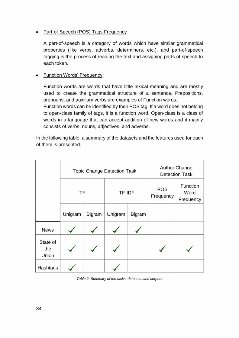
In the following table, a summary of the datasets and the features used for each

of them is presented.

Topic Change Detection Task Author Change

Detection Task

TF TF-IDF POS

Frequency

Function

Word

Frequency

Unigram Bigram Unigram Bigram

News

State of

the

Union

Hashtags

Table 2. Summary of the tasks, datasets, and corpora

35

Preprocessing

Before extracting the features from the data and using them in the algorithm

described in the previous chapter, some preprocessing must be carried out to

make the data ready to use. These pre-processes vary depending on the task

and the dataset.

The following four operations were carried out on the News and the State of the

Union corpora for the topic change task:

Tokenisation

Tokenisation is the process of breaking a stream of text up into smaller

meaningful components called tokens. Since English has inter-word

spaces, this task is mostly straightforward in normal texts like the news

articles or the State of the Union addresses. In Twitter data, however,

because of its noisy nature, tokenisation is not so simple and more

specialised tools might be necessary to carry out the task. We have used

the Stanford tokenizer which is part of the Stanford NLP suite (Toutanova

et al., 2003) for the tokenisation process.

Case Normalisation

We used a very basic text normalisation method, case normalisation, which

makes all the words uniformly upper or lower case.

Removing Stop words

“Stop words” or words in a “stop list” are the most frequently occurring words

in a language (such as “the”, “of”, “and”, etc. in English) that because of their

commonality, have a very low discriminating value (Fox, 1992). Moreover,

these words make up a large fraction of most documents. According to

Francis and Kucera (1982), the ten most frequently occurring words in

English typically account for 20 to 30 percent of the tokens in a document.

Therefore, by eliminating these words, huge amount of space and

computational power are saved. Stop lists usually contain function words

along with some of the most frequent non-function words (also known as

“content words”).

36

We have used the stop list compiled by Salton10 for the SMART information

retrieval system (Salton, 1971) that contains 570 most frequent words in the

English language.

Lemmatisation

Lemmatisation is the process of determining the “lemma” or the common

base form of a word. For grammatical reasons, a word can be seen in

different forms throughout a document. For instance, "walks", "walking", and

"walked" all have the same base form. The goal of lemmatisation is to group

these inflected forms together.

Lemmatisation is a useful tool in topic modelling, as well as other areas like

information retrieval, because usually all the inflected forms a word indicate

the same topic.

The lemmatisation module we used is “LemmaGen”11 (Juršic et al., 2010)

developed initially for C++.

For the authorship change task, extracting the part-of-speech (POS) frequency

was the only necessary preprocessing:

Part-of-speech (POS) Tagging

As explained in the Feature Section, POS tags were used as features in the

authorship change task; therefore, extracting them was a necessary step

for the authorship task.

We have used the Stanford POS tagger (Toutanova et al., 2003) for this

task. Stanford POS tagger uses Penn treebank’s 45 POS tags, including

punctuations (see Gildea and Jurafsky (2002) for the full list).

Using the previously mentioned pre-processes in the authorship task, would

have distorted the data as lemmatisation destroys grammatical variations and

most of the stop words are function words and therefore strong indicators of

writers’ style (see 2.4).

10 Available at www.lextek.com/manuals/onix/stopwords2.html

11 Available at http://lemmatise.ijs.si/

37

Feature Selection

The dimension of the feature vector can become quite large even for small

documents. Some of the elements in the feature vector can be dropped without

affecting the performance of the system. Feature selection is the process of

removing irrelevant features and it had some benefits including the reduction of

computations by reducing the size of the feature vector.

Some of the preprocessing steps explained in the previous section (stop words

removal, lemmatising, and case normalisation) are extensions of feature

selection. However, in this section, we focus on the processes that create a

subset of the features introduced in the Features Section. We compared the

performance obtained with these subsets to that obtained with all the features

to assess the contribution of the feature selection process.

For the topic change task, we used the values of corpus-wide term frequency

(TF) and document frequency (DF) to get a subset of the features that might

contribute more in discriminating the documents, while reducing the feature

vector’s dimension.

In the SOU corpus, we experimented with removing all the terms with DF values

of more than 50, 30, and 10, removing nearly 4%, 8%, and 25% of the features.

Terms with higher values of DF (terms that appear in more documents) tend to

have less discriminating values.

For the hashtags corpus, we took a more aggressive approach and

experimented with removing 99.9%, 99.75%, and 98.9% of the hashtags with

the lowest frequencies across the corpus and reduced the feature vector’s

dimension from over a million to near 1500, 3000, and 13600 respectively. Even

with the largest reduction, the algorithm takes 12 hours to run, which is far from

being online.

We also removed all the hashtags with maximum DF. These hashtags can be

considered the “stop words” for the hashtag corpus. These were mostly sex

related terms, a few indiscriminative hashtags seen in advertisement or spam

tweets (such as “#free”, #win, and “#sale”), and Twitter related hashtags

(#retweet and its abbreviation #rt).

For the author change task, we performed feature selection on the function

words feature and as suggested by Koppel et al. (2009), instead of using all the

function words as features, we experimented with using a feature vector

38

consisting of the top 30, 50, and 100 most frequent function words of the

English language.

Evaluation Methods

As the problem is set in an unsupervised environment, evaluating the results of

the experiments was anticipated to be a big challenge with no universally good

evaluation technique. This is the motivation for creating the synthetic dataset

with known changepoint positions. For the other corpora, we have used a

combination of observing the results to see if they match expectations based

on the real-world events, similar to the one used by Liu et al. (2013), and more

formal methods, explained in this section, to validate the results.


To evaluate the results of the topic change task, we investigated the similarities

between pairs of documents using cosine similarity and Labbé Distance

(Labbé, 2007). A dissimilarity threshold was calculated using the symmetric

Labbé Distance, proposed by Savoy (2015). This threshold is consistent across

all corpora and any transition between two documents that are more dissimilar

than this threshold, is detected as change by our algorithm.

The symmetric Labbé distance, takes the document lengths into account and

can work for documents that do not have the same length. The distance

between the documents 𝐴 and 𝐵 is calculated according to Equation 13, where

𝑛𝐴 indicates the length (number of tokens) of document 𝐴, and 𝑡𝑓𝑖𝐴 and 𝑡𝑓𝑖𝐵

denote the term frequencies of 𝐴 and 𝐵 respectively. The length of the

vocabulary (dictionary) is indicated by ||𝐷||.

𝐷(𝐴, 𝐵) = ∑ |𝑡𝑓𝑖𝐴 − 𝑡𝑓𝑖𝐵

𝑛𝐴𝑛𝐵

|||𝐷||𝑖=1

2𝑛𝐴 (13)

The result is a number between 0 and 1, 0 for identical documents and 1 for

documents that do not share a single term.

Cosine similarity, a vector-based similarity commonly used in text mining and

information retrieval, is calculated by the following relation:

𝐷 (𝐴, 𝐵) = 𝛼 . 𝛽

|𝛼||𝛽|=

∑ 𝛼 𝑖. 𝛽 𝑖 ||𝐷||𝑖=1

√∑ 𝛼 𝑖2

||𝐷||𝑖=1

√∑ 𝛽 𝑖 2||𝐷||𝑖=1

(14)

39

Where 𝛼 and 𝛽 are the feature vectors representing documents 𝐴 and 𝐵 and

||𝐷|| is their size.


To evaluate and compare the performance of the system in the authorship

change detection task, we used clustering, an unsupervised approach

commonly used in evaluating authorship attribution (Baayen et al., 2002; Labbé

and Labbé, 2001; Savoy, 2015). Comparing our system’s performance to that

of supervised classification methods is not reasonable, as these methods have

the advantage of using extra data, such as other speeches by the presidents,

to train the classifiers.

In this task, clustering is the process of grouping documents in a way that the

documents in the same group (cluster) are more likely to have the same author.

We used a hierarchical clustering (HC) that is flexible in the number of clusters,

and gives better visualisation of cluster assignments than non-hierarchical

clustering methods. We used Euclidean distance as the similarity metric. HC

also requires a linkage criterion that determines the distance between sets of

observations as a function of the pairwise distances between observations. We

tried different linkage criteria (single, complete, centroid, and average) and

average linkage yielded the best results. The average linkage criterion defines

the distance between two clusters by the average of the distances between the

elements in the two clusters:

1

|𝐴|. |𝐵|∑ ∑ 𝑑(𝑎, 𝑏) (15)

𝑏∈𝐵𝑎∈𝐴

Where 𝐴 and 𝐵 are the two clusters, 𝑎 and 𝑏 their elements, and 𝑑(𝑎, 𝑏) the

(Euclidean) distance between 𝑎 and 𝑏.

Optimisation Methods

Because the system is intended for an online setting, it needs to be very

efficient. Therefore, we made some modifications to the algorithm and other

parts of the system. The two major bottlenecks of the system were working with

the large feature vector and constructing the dynamic programming table.

To implement the feature vectors, we used a hash table that maps the terms to

their TF or TF-IDF values. Comparing strings with each other and hashing

strings are two time-consuming tasks done quite a lot in the algorithm, and

furthermore, the algorithm does not require the actual terms at any stage.

40

Therefore, to improve the run time, we used an integerised version of the

feature hash table, where the keys are the integer indices of the terms rather

than the actual strings.

The time complexity of constructing the dynamic programming table grows

linearly with each new timestep, as in each timestep a new segmentation

possibility is created. An optimisation method is proposed by the original

authors of the algorithm, Adams and MacKay (2007), which we used here. In

this method, the nodes (possible segmentations) that have a low probability are

ignored in the subsequent timesteps, thus reducing the computation time.

41

5 Results and Analysis

In this chapter, first we provide the results obtained for each corpus using

different features and feature selection processes along with an analysis of

them (Sections 5.1 to 5.3). Then, we present the result of further analysis on

different components of the algorithm (5.4 Sensitivity Analysis).

The News Corpus

The news corpus consisted of 12 documents handpicked to be on six different

topics and since we arranged the documents manually to test the algorithm

(see Table 1 for the arrangement), we expected five changepoints and

therefore the prior probability of change (the 𝑃 (𝑟𝑡 | 𝑟𝑡−1 ) in Equation 2) for this

corpus was set to 5/12.

The TF unigram feature delivered these expectations (Figure 9). In this diagram

(and all the upcoming results diagrams) the horizontal axis is the time including

the name of the document at that timestep, and the vertical axis is the segment

length that has the maximum probability among all possible segment lengths.

Therefore, a segment length of zero denotes a changepoint in the data and the

data between two changepoints belong to the same segment.

Figure 9. Segment Length with maximum probability over time using TF unigrams

Running the algorithm with the TF bigram feature found a new changepoint by

separating the two “fire” articles into two segments (Figure 10).

0

1

2

3

Segm

ent

Len

gth

Time (Documents)

42

Figure 10. Segment Length with maximum probability over time using TF bigrams

This shows that the TF bigram feature is more sensitive than the unigram

feature and the two documents that were previously in one segment are now

categorised into two segments.

Running the algorithm using the TF bigram feature increased the runtime

significantly, from six minutes to an hour, as the size of the dictionary, and

consequently the size of each feature vector, is increased from 2059 to 4496.

Extracting the bigram frequencies was also more time consuming than

extracting unigram frequencies.

The TD-IDF features, as expected, were even more sensitive to the changes in

the documents. The algorithm under the TF-IDF unigram feature (Figure 11),

partitioned that third “fish” article, which was about a family of fish different from

the first two “fish” articles, in a separate segment and also separated the

assaults cases in India ending up with 9 changepoints in total.

Figure 11. Segment Length with maximum probability over time using TFIDF unigrams

The TF-IDF bigram yielded even more changepoints by partitioning the last

three documents in three separate segments (Figure 12).

0

1

2

3

Segm

ent

Len

gth

Time (Documents)

0

1

2

3

Segm

ent

Len

gth

Time (Documents)

43

Figure 12. Segment Length with maximum probability over time using TFIDF bigrams

So, it can be concluded that the features must be chosen depending on the

sensitivity and the level of detail we are interested in. Using TF unigrams, TF

bigrams, TFIDF unigrams, and TFIDF bigrams in this order increases sensitivity

to document differences and also the runtime of the algorithm.

0

1

2

Segm

ent

Len

gth

Time (Documents)

44

The State of the Union (SOU) Corpus

We attempted both the topic change detection and author change detection

tasks on this corpus. While the runtime was not an issue in the previous corpus,

with the increase in number of documents (from 12 to 86) and their average

size (from 920 tokens to 8725), it became an obstacle for this corpus, to the

point that we could not run the bigram TF and TFIDF features.

The value of prior probability of change for the authorship task was set to 14/86

= 0.16, because there were 14 president changes in the 86 speeches. For the

topic change task however, no prior knowledge of the number of changepoints

in topic is available, therefore, we used the same value. Later, we conducted a

sensitivity analysis on the value of prior probability of change and it became

apparent that this value has little to no effect on the joint probability and so we

did not change this initial value assignment (see Section 5.4).


The TF unigram feature did not lead to any change detection among the

documents (Figure 13). To validate these results, we started investigating the

cause by calculating the similarities between the documents in SOU.

We calculated the similarities between each consecutive pair of documents in

the corpus using the cosine similarity measure and the Labbé distance (see

Section 4.5.1 for details). The average cosine similarity in all documents in the

SOU corpus is 0.68. In comparison, documents in the news corpus have an

average similarity of 0.26. This shows that the SOU documents are very similar.

Additionally, using the Labbé distance, a dissimilarity threshold can be defined

for the algorithm. Because in Labbé distance 0 represents identical documents

and 1 represents completely different ones, any similarity higher than a

threshold indicates a change. This dissimilarity threshold was found to be 0.9,

a consistent number for all the tested corpora.

By using this threshold we can validate that the documents in the SOU corpus

are too similar for the algorithm to detect any changepoints. The value of Labbé

distance for all consecutive pair of documents in the SOU are below the

dissimilarity threshold (0.9). Table 3 in the Appendix I illustrates the Labbé

distance and cosine similarity for all pairs of consecutive documents in all the

corpora and whether they were identified as a change or not by the algorithm.

45

Figure 13: Segment Length with maximum probability over time using TF unigram.

0

50

100

RO

34

RO

36

RO

38

RO

40

RO

42

RO

44

TR4

5

TR4

7

TR4

9

TR5

1

EI5

4

EI5

6

EI5

8

EI6

0

KE6

2

KE6

3

JO6

5

JO6

6

JO6

8

NI7

0

NI7

2

NI7

4

FO7

6

CA

78

CA

80

RE8

2

RE8

4

RE8

6

RE8

8

BU

90

BU

91

CL9

3

CL9

5

CL9

7

CL9

9

BU

01

BU

02

BU

04

BU

06

BU

08

OB

10

OB

12

OB

14

Segm

ent

Len

gth

Time (president+year)

0

50

100

RO

34

RO

36

RO

38

RO

40

RO

42

RO

44

TR4

5

TR4

7

TR4

9

TR5

1

EI5

4

EI5

6

EI5

8

EI6

0

KE6

2

KE6

3

JO6

5

JO6

6

JO6

8

NI7

0

NI7

2

NI7

4

FO7

6

CA

78

CA

80

RE8

2

RE8

4

RE8

6

RE8

8

BU

90

BU

91

CL9

3

CL9

5

CL9

7

CL9

9

BU

01

BU

02

BU

04

BU

06

BU

08

OB

10

OB

12

OB

14

Segm

ent

Len

gth


0

50

100

RO

34

RO

36

RO

38

RO

40

RO

42

RO

44

TR4

5

TR4

7

TR4

9

TR5

1

EI5

4

EI5

6

EI5

8

EI6

0

KE6

2

KE6

3

JO6

5

JO6

6

JO6

8

NI7

0

NI7

2

NI7

4

FO7

6

CA

78

CA

80

RE8

2

RE8

4

RE8

6

RE8

8

BU

90

BU

91

CL9

3

CL9

5

CL9

7

CL9

9

BU

01

BU

02

BU

04

BU

06

BU

08

OB

10

OB

12

OB

14

Segm

ent

Len

gth


Figure 14: Segment Length with maximum probability over time using TF-IDF unigram.

Figure 15: Segment Length with maximum probability over time using TF unigram with feature selection.

46

This trend continues even with the TF-IDF unigram feature (Figure 14) that was

much more sensitive in the test corpus. We tried to improve the detection and

runtime by doing a feature selection using the document frequency (DF) count.

We removed all the terms with DF value more than 50, 30, and 10 (see Section

4.4). However, none of these subsets made a difference in the output (Figure

15).


As stated before, the fact that politicians have teams of speech writers affects

the evaluation process of this task. Savoy (2015) has shown that usually there

is a high similarity between the first SOU speech of a president and the

speeches by his predecessor. He speculates that this is due to lack of enough

time to change the speechwriters or for the speechwriters to adapt a new style

of writing.

However, in order to be able to evaluate the system and compare its

performance with that of the baseline, an assumption must be made that each

president represents a cluster and a speech belong to that cluster if and only if

it was delivered by that president. Given the reality of political speech writing,

this assumption leads to very poor performance, however, it is a reasonable

assumption for performance comparison.

Our system’s performance for this task was compared with unsupervised

hierarchical clustering, which can be used as a baseline in the authorship

attribution studies.

5.2.2.1 Function Words Frequency

The function words feature was used after the feature selection process of only

picking the frequency of the most frequent 30, 50, and 100 function words in

English. The results are presented in Figures 16 to 18.

With the naïve authorship assumption stated above, the top 30 function words

feature yielded eight clusters with 29 misclassified instances, an overall

accuracy of 66.3%. The top 50 function words, gave bigger clusters with more

noise, achieving 52.3% accuracy. Finally, the top 100 function words gave a

slightly worse performance, misclassifying 42 instances and achieving 51%

accuracy.

We compared the system’s performance with a hierarchical clustering using the

same features. The dendrograms depicting the hierarchical cluster

47

assignments along with confusion matrices (showing cluster assignments when

13 was chosen as the number of clusters) is presented in Appendix II.

The low accuracy of clustering along with the fact that all the features yield at

least five unknown clusters (clusters that have no majority president to be the

label of that cluster), show that the authorship attribution task on this corpus is

quite challenging.

One reason that our system’s accuracy is much higher than the clustering’s is

that our system has the benefit of segmenting the data sequentially. In our

system two documents can only be clustered into one segment if they are

received one after another. However, in the baseline clustering, documents

from different times can, incorrectly, be clustered together.

Table 2 summarises the accuracy achieved in the hierarchical clustering and

our system using different features. The trends in the accuracy are consistent

in both methods, with the top 30 function words feature yielding the most

accurate results.

5.2.2.2 POS tag Frequency

Figure 19 illustrates the segmentation using the POS tag frequency feature.

Segments (clusters) achieved with this feature are not as smooth as the

previous three features and contain a lot of noise, however, the number of

identified clusters are significantly higher than the other features and this has

led to a higher accuracy (Table 2).

We expected that these noises will be smoothed by the other terms in the

probability calculation (Equation 2); however, the likelihood component’s

absolute value is high enough to dominate the probability completely.

Therefore, irregular segment lengths appear in the diagrams (see Section 5.4

for more details).

Feature Our system’s

Accuracy Clustering’s Accuracy

POS freq. 70% 28%

Top 30 func. Words freq. 66.30% 29%

Top 50 func. Words freq. 52.30% 25.50%

Top 100 func. Words freq. 51% 24.50%

Table 3.Clustering accuracy using different features

48

0

5

10

15

20

25

30

35

RO

34

RO

35

RO

36

RO

37

RO

38

RO

39

RO

40

RO

41

RO

42

RO

43

RO

44

RO

45

TR4

5TR

46

TR4

7TR

48

TR4

9TR

50

TR5

1EI

53

EI5

4EI

55

EI5

6EI

57

EI5

8EI

59

EI6

0K

E61

KE6

2JO

63

KE6

3JO

64

JO6

5JO

65

JO6

6JO

67

JO6

8JO

69

NI7

0N

I71

NI7

2N

I73

NI7

4FO

75

FO7

6FO

77

CA

78

CA

79

CA

80

RE8

1R

E82

RE8

3R

E84

RE8

5R

E86

RE8

7R

E88

BU

89

BU

90

BU

91

BU

91

BU

92

CL9

3C

L94

CL9

5C

L96

CL9

7C

L98

CL9

9C

L20

00

BU

01

BU

01

BU

02

BU

03

BU

04

BU

05

BU

06

BU

07

BU

08

OB

09

OB

10

OB

11

OB

12

OB

13

OB

14

OB

15

Segm

ent

Len

gth


02468

101214161820

RO

34

RO

35

RO

36

RO

37

RO

38

RO

39

RO

40

RO

41

RO

42

RO

43

RO

44

RO

45

TR4

5TR

46

TR4

7TR

48

TR4

9TR

50

TR5

1EI

53

EI5

4EI

55

EI5

6EI

57

EI5

8EI

59

EI6

0K

E61

KE6

2JO

63

KE6

3JO

64

JO6

5JO

65

JO6

6JO

67

JO6

8JO

69

NI7

0N

I71

NI7

2N

I73

NI7

4FO

75

FO7

6FO

77

CA

78

CA

79

CA

80

RE8

1R

E82

RE8

3R

E84

RE8

5R

E86

RE8

7R

E88

BU

89

BU

90

BU

91

BU

91

BU

92

CL9

3C

L94

CL9

5C

L96

CL9

7C

L98

CL9

9C

L20

00

BU

01

BU

01

BU

02

BU

03

BU

04

BU

05

BU

06

BU

07

BU

08

OB

09

OB

10

OB

11

OB

12

OB

13

OB

14

OB

15

Segm

ent

Len

gth


Figure 17: Segment Length with maximum probability over time using top 30 function words frequency.


49

05

101520253035404550

RO

34

RO

35

RO

36

RO

37

RO

38

RO

39

RO

40

RO

41

RO

42

RO

43

RO

44

RO

45

TR4

5TR

46

TR4

7TR

48

TR4

9TR

50

TR5

1EI

53

EI5

4EI

55

EI5

6EI

57

EI5

8EI

59

EI6

0K

E61

KE6

2JO

63

KE6

3JO

64

JO6

5JO

65

JO6

6JO

67

JO6

8JO

69

NI7

0N

I71

NI7

2N

I73

NI7

4FO

75

FO7

6FO

77

CA

78

CA

79

CA

80

RE8

1R

E82

RE8

3R

E84

RE8

5R

E86

RE8

7R

E88

BU

89

BU

90

BU

91

BU

91

BU

92

CL9

3C

L94

CL9

5C

L96

CL9

7C

L98

CL9

9C

L20

00

BU

01

BU

01

BU

02

BU

03

BU

04

BU

05

BU

06

BU

07

BU

08

OB

09

OB

10

OB

11

OB

12

OB

13

OB

14

OB

15

Segm

ent

Len

gth


0

5

10

15

20

25

RO

34

RO

35

RO

36

RO

37

RO

38

RO

39

RO

40

RO

41

RO

42

RO

43

RO

44

RO

45

TR4

5TR

46

TR4

7TR

48

TR4

9TR

50

TR5

1EI

53

EI5

4EI

55

EI5

6EI

57

EI5

8EI

59

EI6

0K

E61

KE6

2JO

63

KE6

3JO

64

JO6

5JO

65

JO6

6JO

67

JO6

8JO

69

NI7

0N

I71

NI7

2N

I73

NI7

4FO

75

FO7

6FO

77

CA

78

CA

79

CA

80

RE8

1R

E82

RE8

3R

E84

RE8

5R

E86

RE8

7R

E88

BU

89

BU

90

BU

91

BU

91

BU

92

CL9

3C

L94

CL9

5C

L96

CL9

7C

L98

CL9

9C

L20

00

BU

01

BU

01

BU

02

BU

03

BU

04

BU

05

BU

06

BU

07

BU

08

OB

09

OB

10

OB

11

OB

12

OB

13

OB

14

OB

15

Segm

ent

Len

gth



Figure 19: Segment Length with maximum probability over time using POS tag frequency.

50

The Hashtag Corpus

The hashtag corpus was a subset of the Twitter corpus that only includes the

hashtags of the tweets. All the data from one day are aggregated into one

document and the corpus spans 30 days from 18th of April to 18th of May, 2015.

Given that we were only working with hashtags, the bigram TF and TF-IDF

features were not applicable in this corpus.

No prior knowledge over the number of changepoints is available for this

corpus; however, as mentioned before, the likelihood value dominates the joint

probability calculations and the value of the prior probability has no effect on

the change detection.

Given the quite large dimension of the feature vector (over a million), feature

selection was necessary for this corpus. We removed the top 40 frequent

hashtags and experimented with removing the least frequent ones by removing

the hashtags that occur less than 100, 500, or 1000 times (see Section 4.4 for

more details).

The results of using the TF unigram feature for the hashtags with the above

frequencies are presented in Figures 20 to 22.

0

1

2

3

4

Ap

-18

Ap

-19

Ap

-20

Ap

-21

Ap

-22

Ap

-23

Ap

-24

Ap

-25

Ap

-26

Ap

-27

Ap

-28

Ap

-29

Ap

-30

Ma-

01

Ma-

02

Ma-

03

Ma-

04

Ma-

05

Ma-

06

Ma-

07

Ma-

08

Ma-

09

Ma-

10

Ma-

11

Ma-

12

Ma-

13

Ma-

14

Ma-

15

Ma-

16

Ma-

17

Segm

ent

Len

gth

Time

Figure 20. Segment Length with maximum probability using Hashtags with over 100 Frequency

51



As it can be seen from the diagrams, removing hashtags occurring less than

500 and 1000 times lead to a very sensitive change detection, partitioning each

document to a separate segment (with an exception of one). The Labbé

distance similarity validates these results.

Figure 23. Segment Length with maximum probability using TFIDF values of the Hashtags with over 100

Frequency

0

1

2

Ap

-18

Ap

-19

Ap

-20

Ap

-21

Ap

-22

Ap

-23

Ap

-24

Ap

-25

Ap

-26

Ap

-27

Ap

-28

Ap

-29

Ap

-30

Ma-

01

Ma-

02

Ma-

03

Ma-

04

Ma-

05

Ma-

06

Ma-

07

Ma-

08

Ma-

09

Ma-

10

Ma-

11

Ma-

12

Ma-

13

Ma-

14

Ma-

15

Ma-

16

Ma-

17

Segm

ent

Len

gth

Time

0

1

Ap

-18

Ap

-19

Ap

-20

Ap

-21

Ap

-22

Ap

-23

Ap

-24

Ap

-25

Ap

-26

Ap

-27

Ap

-28

Ap

-29

Ap

-30

Ma-

01

Ma-

02

Ma-

03

Ma-

04

Ma-

05

Ma-

06

Ma-

07

Ma-

08

Ma-

09

Ma-

10

Ma-

11

Ma-

12

Ma-

13

Ma-

14

Ma-

15

Ma-

16

Ma-

17

Segm

ent

Len

gth

Time

0

1

Ap

-18

Ap

-19

Ap

-20

Ap

-21

Ap

-22

Ap

-23

Ap

-24

Ap

-25

Ap

-26

Ap

-27

Ap

-28

Ap

-29

Ap

-30

Ma-

01

Ma-

02

Ma-

03

Ma-

04

Ma-

05

Ma-

06

Ma-

07

Ma-

08

Ma-

09

Ma-

10

Ma-

11

Ma-

12

Ma-

13

Ma-

14

Ma-

15

Ma-

16

Ma-

17

Segm

ent

Len

gth

Time

52

Considering this observation, we ran TF-IDF unigram only for hashtags with

higher than 100 frequencies and as expected, the algorithm still considered all

transitions as change (Figure 23).

Initially, we expected that we can match the changes in Figure 20 with the real-

world events, however, by observing the data it becomes apparent that this is

not straightforward for two reasons. Firstly, the changes may reflect multiple

events in real-world and second, the changes in trending topics does not

necessarily reflect the real-world events.

For instance, we hypothesized that the clear change on 25th of April, reflects

Nepal’s earthquake. However, although the #nepalearthquake became a

popular hashtag on that day (ranking at 14), the change is more affected by two

new hashtags (ranking 1 and 2), #whereiwaswhenzaynquit and #followmejosh,

none of which reflect a real-world event12.

The results obtained on this corpus are far from helpful even for the first feature

that shows some changes. In order to get any useful information, modifications

must be made to the current setting.

Using more data in the features, i.e. incorporating hashtags with less frequency

may help, however, it will make the runtime much worse. A possibly better

approach involves introducing a target for the change detection. In this

approach, instead of considering all the tweets in a day, only tweets containing

a term from a group of keywords will be considered. For instance, when tracking

a specific disease, we can compile a list of relevant keywords consisting of the

common symptoms of that disease, and only use the tweets that include a word

from that list as the data. This idea is currently being tested.

Sensitivity Analysis over the Prior Probability

As it was mentioned above, finding the right value for prior probability of change

becomes an issue in real-world applications if no prior knowledge about the

number of changepoints is known or can be guessed. So we were interested to

see how much this value contributes to the calculation of the joint probability

(Equation 2).

12 The first hashtag relates to the event of a pop singer, Zayn Malik, quitting from his band

that happened a month before in March, however, the hashtag first emerged on 25th of April.

The second hashtag is a request from people to another member of that band to follow them

on Twitter.

53

We conducted a sensitivity analysis on the value of this prior probability and

found out that it has no effect on the joint probability. Changing its value from

0.001 to 0.999 had no effect on the outcome in the test or SOU corpora.

In fact, among the three terms in Equation 2, the likelihood is the biggest

contributor to the overall probability to the extent that it renders the two other

terms virtually obsolete. This results in losing the effects of the prior probability,

which incorporates domain knowledge, and the probability from the preceding

timestep, which reduces the noise and makes segmentation smoother. This is

the main problem with the current likelihood model that we are addressing (See

6.1 Future Work).

54

6 Conclusion and Future Work

Conclusion

Text mining is the process of extracting useful information from textual data and

has many applications in numerous disciplines. As web social media, blogging,

and online forums can provide vast amounts of user generated content that can

reflect the thoughts and opinions of the users, their topics of interest, and much

more information about the society as a whole, it is an invaluable source for text

mining applications.

One aspect of text mining is the temporal analysis of the documents, an aspect

that is the focus of a few studies. If a stream of text is analysed over time,

interesting trends such as changes in topics, meanings of words, or sentiments

over time can be revealed. Timely detection of changes in the topic trends or

simply the use of language on social media can lead to early discovery of

threads to public safety such as epidemic outbreaks.

To be able to achieve this, the change detection must be efficient and capable

of processing the data in real-time as they become available. In this research,

we adapted an online Bayesian change detection algorithm developed by

Adams and Mackay (2007), which was designed for real-valued data, to textual

data and used it to detect changes in a stream of textual data over time.

Different tasks can be attempted using this tool; we have considered two tasks

of detecting changes in the topic, similar to the unsupervised topic

segmentation task, and detecting changes in the author of the documents,

similar to the unsupervised authorship attribution task.

In order to adapt the algorithm to text, we developed a new likelihood model for

it based on the principle of lexical cohesion and devised a set of features to

represent the documents based on the tasks. A number of features selection

processes were also necessary in order to make the system feasible to run.

Like any unsupervised study, evaluating the research was a big challenge. In

addition to observing the changes, and matching them to real-world events, we

used more formal evaluation approaches and used similarity measures to

validate the topic change task and hierarchical clustering to evaluate the

authorship change task.

In the test dataset, which has few short length documents, the system performs

well in the topic change task. Using this corpus, it also became apparent which

55

features are more sensitive to the changes in the documents. Using unigrams

term frequency, bigrams term frequency, TF-IDF unigrams, and TF-IDF

bigrams, in this order, increases algorithm’s sensitivity to document differences

at the cost of higher run time.

In the State of the Union corpus that was used for both tasks, the algorithm did

not perform as good as the test corpus. In the topic change task, the unigram

features could not detect any changes in the topic, even with some feature

selections. This is largely due to the high similarity between the documents in

this corpus, which was validated using two similarity measures. Given the size

of data, running the algorithm with the more sensitive bigram features was not

feasible.

In the authorship change task, our systems performs better than the baseline,

however, its performance is still poor. This is largely due to lack of knowledge

about the true authors behind the State of the Union speeches. This task was

more a proof of concept, showing the versatile applications of changepoint

detection on textual data and how the same algorithm can be used for two

distinct tasks with only changing the features.

Finally, the hashtag corpus proved to be too noisy for the algorithm to extract

any useful information and it consistently detected change in all timestep using

most features. As a solution, we propose a more targeted change detection.

This work has shown that an online Bayesian change detection previously used

on real-valued data is in fact applicable to textual data and can be used as a

temporal text mining tool. However, it needs major modifications to be able to

deliver its main objective of being a real-time indicator of change and be useful

in tracking issues of interest such as progression of an epidemic on social

media. It was also shown that the algorithm has the potential of being applied

in multiple domains and tasks with only changes in preprocessing and feature

extraction.

Towards an Online Setting

There is one aspect of the current system that forces it to run only in an offline

setting: the need for a corpus-wide dictionary of all the unique words in the

corpus, used in the likelihood model. To solve this issue and make the algorithm

runnable online, we propose some ideas that we will implement when

continuing this research.

56

A simple solution is using a normal dictionary or lexicon of the English language

as this corpus-wide dictionary. This solution can be utilised when working with

texts that use a standard language like news articles or the State of the Union

addresses. These texts normally do not contain any words that are not found in

a dictionary other than proper nouns. However, in social media data, which is

full of non-standard words, this solution is not as helpful or necessitates major

normalisations of the data. Other possible solution is modifying the model to

work with a dynamic dictionary that grows as new data becomes available.

There are other parts in the current system that are not online, however, they

are optional components. For instance, the TF-IDF features are only extractable

offline, when the entire corpus is available to calculate document frequency.

The feature selection process for the topic change task also exploited the entire

corpus to calculate corpus-wide term frequency and document frequency,

something that cannot be done in an online setting.

TF-IDF features are more sensitive to change, and therefore, more useful in

some applications. Moreover, feature selection helps making the algorithm

more efficient; therefore, it is worthwhile to retain these components in an online

setting. This can be achieved by utilising an external training corpus. The values

of DF or corpus-wide TF can be calculated from an external corpus that is

similar to the test corpus.

As a final note, the runtime of the algorithm on large datasets, like tweets, is not

acceptable in an online system. Further optimisation is necessary to address

this issue. Wilson et al. (2010) suggest a more efficient node pruning method

for this algorithm that we have not yet incorporated in this research and will

consider in the future, in order to make the algorithm more efficient.

Future Work

Apart from the modifications proposed in the previous section, the foremost

priority of the research now is changing the likelihood model. We want to utilise

the models commonly used in topic segmentation in the current algorithm to

produce a better model. Currently in the likelihood model, one multinomial

distribution represents the lexical cohesion in the segment. One of the first

changes we intend to apply on the likelihood is turning this into a mixture model

to capture different properties of the segment’s lexicon.

Despite their differences, all segments with different topics share a portion of

their lexicon that can be separated from the unique portion to yield a more

accurate model. By using a mixture model, we can have a multinomial

57

component to represent the common portion of the lexicon and another

component or multiple other components to represent the unique portions of

the lexicon, representing multiple topics. The change detection in this model is

detecting the changes in either the proportions of these components or the

distributions of the unique components.

After changing the model, we will reattempt the Twitter corpus, and examine

more feature selection options and the targeted approach discussed in Section

5.3 in order to make useful detections on Twitter.

The authorship attribution task can also be attempted on the Twitter corpus,

given the few number of studies in this area. For this task, further research and

experiment on the type of features and the feature selection process is

necessary as Twitter presents the new challenge of determining the author of

short length documents.

58

7 References

Abbasi, A., & Chen, H. (2005). Applying authorship analysis to extremist-group web

forum messages. Intelligent Systems, IEEE, 20(5), 67-75.

Abel, F., Gao, Q., Houben, G. J., & Tao, K. (2011). Analysing user modelling on twitter

for personalized news recommendations. In User Modelling, Adaption and

Personalization (pp. 1-12). Springer Berlin Heidelberg.

About.twitter.com. (2015). About Twitter, Inc. | About. Retrieved 1 June 2015, from

https://about.twitter.com/company.

Adams, R. P., & MacKay, D. J. (2007). Bayesian online changepoint detection. arXiv

preprint arXiv: 0710.3742.

Andrieu, C., De Freitas, N., Doucet, A., & Jordan, M. I. (2003). An introduction to

MCMC for machine learning. Machine learning, 50(1-2), 5-43.

Ardon, S., Bagchi, A., Mahanti, A., Ruhela, A., Seth, A., Tripathy, R. M., & Triukose,

S. (2011). Spatio-temporal analysis of topic popularity in twitter. arXiv preprint

arXiv:1111.2904.

Argamon, S., & Levitan, S. (2005). Measuring the usefulness of function words for

authorship attribution. In ACH/ALLC.

Argamon, S., Koppel, M., Pennebaker, J. W., & Schler, J. (2009). Automatically

profiling the author of an anonymous text. Communications of the ACM, 52(2), 119-

123.

Baayen, H., Van Halteren, H., & Tweedie, F. (1996). Outside the cave of shadows:

Using syntactic annotation to enhance authorship attribution. Literary and Linguistic

Computing, 11(3), 121-132.

Baayen, H., van Halteren, H., Neijt, A., & Tweedie, F. (2002). An experiment in

authorship attribution. In 6th JADT (pp. 29-37).

Bansal, N., & Koudas, N. (2007). Blogscope: a system for online analysis of high

volume text streams. In Proceedings of the 33rd international conference on Very large

data bases (pp. 1410-1413). VLDB Endowment.

Barlow, J. S., Creutzfeldt, O. D., Michael, D., Houchin, J., & Epelbaum, H. (1981).

Automatic adaptive segmentation of clinical EEGs. Electroencephalography and

Clinical Neurophysiology, 51(5), 512-525.

Barry, D., & Hartigan, J. A. (1992). Product partition models for change point

problems. The Annals of Statistics, 260-279.

59

Basseville, M., & Nikiforov, I. V. (1993). Detection of abrupt changes: theory and

application (Vol. 104). Englewood Cliffs: Prentice Hall.

Baxter, R. A., & Oliver, J. J. (1996). The kindest cut: minimum message length

segmentation. In Algorithmic Learning Theory (pp. 83-90). Springer Berlin Heidelberg.

Beaulieu, C., Chen, J., & Sarmiento, J. L. (2012). Change-point analysis as a tool to

detect abrupt climate variations. Philosophical Transactions of the Royal Society A:

Mathematical, Physical and Engineering Sciences, 370(1962), 1228-1249.

Bird, S., Klein, E., & Loper, E. (2009). Natural language processing with Python.

"O'Reilly Media, Inc.".

Bodenstein, G., & Praetorius, H. M. (1977). Feature extraction from the

electroencephalogram by adaptive segmentation. Proceedings of the IEEE, 65(5),

642-652.

Bollen, J., Mao, H., & Pepe, A. (2011). Modeling public mood and emotion: Twitter

sentiment and socio-economic phenomena. In ICWSM.

Bollen, J., Mao, H., & Zeng, X. (2011). Twitter mood predicts the stock market. Journal

of Computational Science, 2(1), 1-8.

Bovolo, F., Bruzzone, L., & Marconcini, M. (2008). A novel approach to unsupervised

change detection based on a semisupervised SVM and a similarity measure.

Geoscience and Remote Sensing, IEEE Transactions on, 46(7), 2070-2082.

Boyd, D., Golder, S., & Lotan, G. (2010). Tweet, tweet, retweet: Conversational

aspects of retweeting on twitter. In System Sciences (HICSS), 2010 43rd Hawaii

International Conference on (pp. 1-10). IEEE.

Brodsky, E., & Darkhovsky, B. S. (1993). Nonparametric methods in change point

problems (No. 243). Springer.

Carlin, B. P., Gelfand, A. E., & Smith, A. F. (1992). Hierarchical Bayesian analysis of

changepoint problems. Applied statistics, 389-405.

Cataldi, M., Di Caro, L., & Schifanella, C. (2010). Emerging topic detection on twitter

based on temporal and social terms evaluation. In Proceedings of the Tenth

International Workshop on Multimedia Data Mining (p. 4). ACM.

Chaski, C. E. (2005). Who’s at the keyboard? Authorship attribution in digital

evidence investigations. International Journal of Digital Evidence, 4(1), 1-13.

Chen, J., & Gupta, A. K. (2011). Parametric statistical change point analysis: with

applications to genetics, medicine, and finance. Springer.

60

Chib, S. (1998). Estimation and comparison of multiple change-point models. Journal

of econometrics, 86(2), 221-241.

Chopin, N. (2007). Dynamic detection of change points in long time series. Annals of

the Institute of Statistical Mathematics, 59(2), 349-366.

Collier, N., & Doan, S. (2011). Syndromic classification of twitter messages. arXiv

preprint arXiv: 1110.3094.

Csörgö, M., & Horváth, L. (1997). Limit theorems in change-point analysis. New York:

Wiley.

Denison, D. G. T., & Holmes, C. C. (2001). Bayesian partitioning for estimating disease

risk. Biometrics, 143-149.

Doucet, A., De Freitas, N., & Gordon, N. (Eds.). (2001). Sequential Monte Carlo

methods in practice. Springer.

Eisenstein, J., & Barzilay, R. (2008). Bayesian unsupervised topic segmentation.

In Proceedings of the Conference on Empirical Methods in Natural Language

Processing (pp. 334-343). Association for Computational Linguistics.

Fearnhead, P. (2006). Exact and efficient Bayesian inference for multiple changepoint

problems. Statistics and computing, 16(2), 203-213.

Fearnhead, P., & Liu, Z. (2007). On‐line inference for multiple changepoint

problems. Journal of the Royal Statistical Society: Series B (Statistical

Methodology), 69(4), 589-605.

Feldman, R., & Sanger, J. (2007). The text mining handbook: advanced approaches

in analyzing unstructured data. Cambridge University Press.

Fitzgibbon, L. J., Dowe, D. L., & Allison, L. (2002). Change-point estimation using new

minimum message length approximations. In PRICAI 2002: Trends in Artificial

Intelligence (pp. 244-254). Springer Berlin Heidelberg.

Fox, C. J. (1992). Lexical Analysis and Stoplists.

Francis, W., & Kucera, H. (1982). Frequency analysis of English usage.

Frantzeskou, G., Stamatatos, E., Gritzalis, S., Chaski, C. E., & Howald, B. S. (2007).

Identifying authorship by byte-level n-grams: The source code author profile (scap)

method. International Journal of Digital Evidence, 6(1), 1-18.

Gamon, M. (2004). Linguistic correlates of style: authorship classification with deep

linguistic analysis features. In Proceedings of the 20th international conference on

Computational Linguistics (p. 611). Association for Computational Linguistics.

61

Geman, S., & Geman, D. (1984). Stochastic relaxation, Gibbs distributions, and the

Bayesian restoration of images. Pattern Analysis and Machine Intelligence, IEEE

Transactions on, (6), 721-741.

Gildea, D., & Jurafsky, D. (2002). Automatic labelling of semantic roles. Computational

linguistics, 28(3), 245-288.

Gordon, N. J., Salmond, D. J., & Smith, A. F. (1993). Novel approach to nonlinear/non-

Gaussian Bayesian state estimation. In IEE Proceedings F (Radar and Signal

Processing) (Vol. 140, No. 2, pp. 107-113). IET Digital Library.

Green, P. J. (1995). Reversible jump Markov chain Monte Carlo computation and

Bayesian model determination. Biometrika, 82(4), 711-732.

Gustafsson, F., & Gustafsson, F. (2000). Adaptive filtering and change detection (Vol.

1). New York: Wiley.

Habib, T., Inglada, J., Mercier, G., & Chanussot, J. (2009). Support vector reduction in

SVM algorithm for abrupt change detection in remote sensing. Geoscience and

Remote Sensing Letters, IEEE, 6(3), 606-610.

Hsu, D. A. (1977). Tests for variance shift at an unknown time point. Applied Statistics,

279-284.

Huang, J., Thornton, K. M., & Efthimiadis, E. N. (2010). Conversational tagging in

twitter. In Proceedings of the 21st ACM conference on Hypertext and hypermedia (pp.

173-178). ACM.

Hutwagner, M. L., Thompson, M. W., Seeman, G. M., & Treadwell, T. (2003). The

bioterrorism preparedness and response early aberration reporting system

(EARS). Journal of Urban Health, 80(1), i89-i96.

Jansen, B. J., Zhang, M., Sobel, K., & Chowdury, A. (2009). Twitter power: Tweets as

electronic word of mouth. Journal of the American society for information science and

technology, 60(11), 2169-2188.

Java, A., Song, X., Finin, T., & Tseng, B. (2007). Why we twitter: understanding

microblogging usage and communities. In Proceedings of the 9th WebKDD and 1st

SNA-KDD 2007 workshop on Web mining and social network analysis (pp. 56-65).

ACM.

Juršic, M., Mozetic, I., Erjavec, T., & Lavrac, N. (2010). Lemmagen: Multilingual lemmatisation with induced ripple-down rules. Journal of Universal Computer Science, 16(9), 1190-1214.

Kennedy, A., & Inkpen, D. (2006). Sentiment classification of movie reviews using

contextual valence shifters. Computational Intelligence, 22(2), 110-125.

62

Koop, G. M., & Potter, S. (2004). Forecasting and estimating multiple change-point

models with an unknown number of change points.

Koppel, M., Schler, J., & Argamon, S. (2009). Computational methods in authorship

attribution. Journal of the American Society for information Science and

Technology, 60(1), 9-26.

Koppel, M., Schler, J., & Argamon, S. (2011). Authorship attribution in the

wild.Language Resources and Evaluation, 45(1), 83-94.

Kramer, A. D. (2010). An unobtrusive behavioral model of gross national happiness.

In Proceedings of the SIGCHI Conference on Human Factors in Computing

Systems (pp. 287-290). ACM.

Kullback, S., & Leibler, R. A. (1951). On information and sufficiency. The Annals of

Mathematical Statistics, 79-86.

Kunneman, F. A., Liebrecht, C. C., & van den Bosch, A. P. J. (2014). The (Un)

Predictability of Emotional Hashtags in Twitter.

Kwak, H., Lee, C., Park, H., & Moon, S. (2010, April). What is Twitter, a social network

or a news media?. In Proceedings of the 19th international conference on World Wide

Web (pp. 591-600). ACM.

Labbé, C., & Labbé, D. (2001). Inter-textual distance and authorship attribution

Corneille and Molière. Journal of Quantitative Linguistics, 8(3), 213-231.

Labbé, D. (2007). Experiments on authorship attribution by intertextual distance in

English*. Journal of Quantitative Linguistics, 14(1), 33-80.

Lampos, V., & Cristianini, N. (2010). Tracking the flu pandemic by monitoring the social

web. In Cognitive Information Processing (CIP), 2010 2nd International Workshop

on (pp. 411-416). IEEE.

Lampos, V., De Bie, T., & Cristianini, N. (2010). Flu detector-tracking epidemics on

Twitter. In Machine Learning and Knowledge Discovery in Databases (pp. 599-602).

Springer Berlin Heidelberg.

Lampos, V., Preotiuc-Pietro, D., & Cohn, T. (2013). A user-centric model of voting

intention from Social Media. In ACL (1) (pp. 993-1003).

Layton, R., Watters, P., & Dazeley, R. (2010a). Authorship attribution for twitter in 140

characters or less. In Cybercrime and Trustworthy Computing Workshop (CTC), 2010

Second (pp. 1-8). IEEE.

63

Layton, R., Watters, P., & Dazeley, R. (2010b). Automatically determining phishing

campaigns using the uscap methodology. In eCrime Researchers Summit (eCrime),

2010 (pp. 1-8). IEEE.

Layton, R., Watters, P., & Dazeley, R. (2012). Unsupervised authorship analysis of

phishing webpages. In Communications and Information Technologies (ISCIT), 2012

International Symposium on (pp. 1104-1109). IEEE.

Lim, Kar Wai, and Wray Buntine. "Twitter Opinion Topic Model: Extracting Product

Opinions from Tweets by Leveraging Hashtags and Sentiment Lexicon." (2014).

Liu, S., Yamada, M., Collier, N., & Sugiyama, M. (2013). Change-point detection in

time-series data by relative density-ratio estimation. Neural Networks, 43, 72-83.

Luhn, H. P. (1957). A statistical approach to mechanized encoding and searching of

literary information. IBM Journal of research and development, 1(4), 309-317.

Madsen, H. (2007). Time series analysis. Boca Raton, Florida: Chapman & Hall/CRC

Press.

Mehrotra, R., Sanner, S., Buntine, W., & Xie, L. (2013). Improving lda topic models for

microblogs via tweet pooling and automatic labelling. In Proceedings of the 36th

international ACM SIGIR conference on Research and development in information

retrieval (pp. 889-892). ACM.

Mellor, J., & Shapiro, J. (2013). Thompson Sampling in Switching Environments with

Bayesian Online Change Detection. In Proceedings of the Sixteenth International

Conference on Artificial Intelligence and Statistics (pp. 442-450).

Mosteller, F., & Wallace, D. (1964). Inference and disputed authorship: The Federalist.

Naaman, M., Boase, J., & Lai, C. H. (2010). Is it really about me?: message content in

social awareness streams. In Proceedings of the 2010 ACM conference on Computer

supported cooperative work (pp. 189-192). ACM.

Oh, S. M., Rehg, J. M., & Dellaert, F. (2006). Parameterized duration modelling for

switching linear dynamic systems. In Computer Vision and Pattern Recognition, 2006

IEEE Computer Society Conference on (Vol. 2, pp. 1694-1700). IEEE.

Oliver, J. J., Baxter, R. A., & Wallace, C. S. (1998). Minimum message length

segmentation. In Research and Development in Knowledge Discovery and Data

Mining (pp. 222-233). Springer Berlin Heidelberg.

Page, E. S. (1954). Continuous inspection schemes. Biometrika, 100-115.

Pang, B., Lee, L., & Vaithyanathan, S. (2002). Thumbs up?: sentiment classification

using machine learning techniques. In Proceedings of the ACL-02 conference on

64

Empirical methods in natural language processing-Volume 10(pp. 79-86). Association

for Computational Linguistics.

Paquet, U. (2007). Empirical Bayesian change point detection. Graphical

Models, 1995, 1-20.

Paul, M. J., & Dredze, M. (2011). You are what you Tweet: Analyzing Twitter for public

health. In ICWSM (pp. 265-272).

Pillay, S. R., & Solorio, T. (2010). Authorship attribution of web forum posts. In eCrime

Researchers Summit (eCrime), 2010 (pp. 1-7). IEEE.

Preotiuc-Pietro, D., & Cohn, T. (2013). A temporal model of text periodicities using

Gaussian Processes. In EMNLP (pp. 977-988).

Raftery, A. E., & Akman, V. E. (1986). Bayesian analysis of a Poisson process with a

change-point. Biometrika, 85-89.

Rajaraman, A., & Ullman, J. D. (2011). Mining of massive datasets. Cambridge

University Press.

Reeves, J., Chen, J., Wang, X. L., Lund, R., & Lu, Q. Q. (2007). A review and

comparison of changepoint detection techniques for climate data. Journal of Applied

Meteorology and Climatology, 46(6), 900-915.

Ritter, A., Clark, S., & Etzioni, O. (2011). Named entity recognition in tweets: an

experimental study. In Proceedings of the Conference on Empirical Methods in Natural

Language Processing (pp. 1524-1534). Association for Computational Linguistics.

Romero, D. M., Meeder, B., & Kleinberg, J. (2011). Differences in the mechanics of

information diffusion across topics: idioms, political hashtags, and complex contagion

on twitter. In Proceedings of the 20th international conference on World Wide Web (pp.

695-704). ACM.

Roth, T., Sprau, P., Naguib, M., & Amrhein, V. (2012). Sexually selected signaling in

birds: a case for Bayesian change-point analysis of behavioral routines. The

Auk, 129(4), 660-669.

Sakaki, T., Okazaki, M., & Matsuo, Y. (2010). Earthquake shakes Twitter users: real-

time event detection by social sensors. In Proceedings of the 19th international

conference on World Wide Web (pp. 851-860). ACM.

Salton, G. (1971). The SMART retrieval system—experiments in automatic document

processing.

Savoy, J. (2015). Text clustering: An application with the State of the Union

addresses. Journal of the Association for Information Science and Technology.

65

Shogan, C. J. (2011). President's State of the Union Address: Tradition, Function, and

Policy Implications. DIANE Publishing.

Sparck Jones, K. (1972). A statistical interpretation of term specificity and its

application in retrieval. Journal of documentation, 28(1), 11-21.

Stephens, D. A. (1994). Bayesian retrospective multiple-changepoint identification.

Applied Statistics, 159-178.

Takahashi, T., Tomioka, R., & Yamanishi, K. (2011). Discovering emerging topics in

social streams via link anomaly detection. In Data Mining (ICDM), 2011 IEEE 11th

International Conference on (pp. 1230-1235). IEEE.

Thelwall, M., & Prabowo, R. (2007). Identifying and characterizing public science‐

related fears from RSS feeds. Journal of the American Society for Information Science

and Technology, 58(3), 379-390.

Toutanova, K., Klein, D., Manning, C. D., & Singer, Y. (2003). Feature-rich part-of-

speech tagging with a cyclic dependency network. In Proceedings of the 2003

Conference of the North American Chapter of the Association for Computational

Linguistics on Human Language Technology-Volume 1 (pp. 173-180). Association for

Computational Linguistics.

Viswanathan, M., Wallace, C. S., Dowe, D. L., & Korb, K. B. (1999). Finding Outpoints

in Noisy Binary Sequences—A Revised Empirical Evaluation. In Advanced Topics in

Artificial Intelligence (pp. 405-416). Springer Berlin Heidelberg.

Wallace, C. S. (2005). Statistical and inductive inference by minimum message length.

New York: Springer.

Wang, Y., Wu, C., Ji, Z., Wang, B., & Liang, Y. (2011). Non-parametric change-point

method for differential gene expression detection. PloS one, 6(5), e20060.

Whiteley, N., Andrieu, C., & Doucet, A. (2011). Bayesian computational methods for

inference in multiple change-points models.

Wigand, F. D. L. (2010). Twitter in government: Building relationships one tweet at a

time. In Information Technology: New Generations (ITNG), 2010 Seventh International

Conference on (pp. 563-567). IEEE.

Wilson, R. C., Nassar, M. R., & Gold, J. I. (2010). Bayesian online learning of the

hazard rate in change-point problems. Neural computation, 22(9), 2452-2476.

Wu, S., Hofman, J. M., Mason, W. A., & Watts, D. J. (2011a). Who says what to whom

on Twitter. In Proceedings of the 20th international conference on World Wide

Web (pp. 705-714). ACM.

66

Wu, S., Tan, C., Kleinberg, J. M., & Macy, M. W. (2011b). Does Bad News Go Away

Faster?. In ICWSM.

Xuan, X., & Murphy, K. (2007). Modelling changing dependency structure in

multivariate time series. In Proceedings of the 24th international conference on

Machine learning (pp. 1055-1062). ACM.

Yamanishi, K., & Takeuchi, J. I. (2002). A unifying framework for detecting outliers and

change points from non-stationary time series data. In Proceedings of the eighth ACM

SIGKDD international conference on Knowledge discovery and data mining (pp. 676-

681). ACM.

Yang, J., & Leskovec, J. (2011). Patterns of temporal variation in online media.

In Proceedings of the fourth ACM international conference on Web search and data

mining (pp. 177-186). ACM.

Zhao, Y., & Zobel, J. (2005). Effective and scalable authorship attribution using

function words. In Information Retrieval Technology (pp. 174-189). Springer Berlin

Heidelberg.

Zheng, R., Li, J., Chen, H., & Huang, Z. (2006). A framework for authorship

identification of online messages: Writing‐style features and classification

techniques. Journal of the American Society for Information Science and

Technology, 57(3), 378-393.

67

8 List of Figures

Figure 1. Normalized frequencies of the ten chosen keywords ...................... 18

Figure 2. Change-point score obtained by Liu et al. (2013) is plotted and the

four occurrences of important real-world events show the development of this

news story ...................................................................................................... 18

Figure 3. Segment Length against time at time 1 (Left) - Segment Length

against time at time 2 (Right) ......................................................................... 21

Figure 4. Segment Length against time at time 3 (Left) - Segment Length

against time at time 7 (Right) ......................................................................... 22

Figure 5. Joint probabilities at time 3 ............................................................. 22

Figure 6. Possible node transitions from timestep 2 to 3 ............................... 24

Figure 7. The Bayesian Network showing the conditional dependency of

model parameters .......................................................................................... 26

Figure 8. Algorithm psudo-code ..................................................................... 29

Figure 9. Segment Length with maximum probability over time using TF

unigrams ........................................................................................................ 41

Figure 10. Segment Length with maximum probability over time using TF

bigrams .......................................................................................................... 42

Figure 11. Segment Length with maximum probability over time using TFIDF

unigrams ........................................................................................................ 42

Figure 12. Segment Length with maximum probability over time using TFIDF

bigrams .......................................................................................................... 43

Figure 13: Segment Length with maximum probability over time using TF

unigram. ......................................................................................................... 45

Figure 14: Segment Length with maximum probability over time using TF-IDF

unigram. ......................................................................................................... 45

Figure 15: Segment Length with maximum probability over time using TF

unigram with feature selection. ...................................................................... 45

68

Figure 16:Segment Length with maximum probability over time using top 50

function words frequency. .............................................................................. 48

Figure 17: Segment Length with maximum probability over time using top 30


Figure 18:Segment Length with maximum probability over time using top 100


Figure 19:Segment Length with maximum probability over time using POS tag

frequency. ...................................................................................................... 49

Figure 20. Segment Length with maximum probability using Hashtags with

over 100 Frequency ....................................................................................... 50


over 500 Frequency ....................................................................................... 51


over 1000 Frequency ..................................................................................... 51

Figure 23. Segment Length with maximum probability using TFIDF values of

the Hashtags with over 100 Frequency .......................................................... 51

Figure 24. Dendrogram (similarity vs clusters) depicting hierarchical cluster

assignments using POS tag frequency .......................................................... 73

Figure 25 . Dendrogram (similarity vs clusters) depicting hierarchical cluster

assignments using the top 30 function words frequency ................................ 73

Figure 26: Dendrogram (similarity vs clusters) depicting hierarchical cluster

assignments using the top 50 function words frequency ................................ 73

Figure 27: Dendrogram (similarity vs clusters) depicting hierarchical cluster

assignments using the top 100 function words frequency. ............................. 73

69

9 List of Tables

Table 1. The NEWS corpus document arrangement showing topics and

expected changepoints .................................................................................. 30

Table 2. Summary of the tasks, datasets, and corpora .................................. 34

Table 3.Clustering accuracy using different features ..................................... 47

Table 4. The values of cosine similarity and Labbé Distance between two

subsequent documents at the first 37 timesteps (excluding time 0) in all the

corpora. The colour green shows the timesteps detected as change ............ 70

Table 5. Confusion Matrix showing cluster assignments and actual labels using

POS tag frequency (accuracy: 28%) .............................................................. 71


30 most frequent function words frequency (accuracy: 29%) ........................ 71


50 most frequent function words frequency (accuracy: 25.5%)...................... 72


100 most frequent function words frequency (accuracy: 24.5%) ................... 72

70

10 Appendix I – Similarity Measures

SUO Hashtags News

Timestep COSINE LABBE COSINE LABBE COSINE LABBE

1 0.637702 0.600316 0.208674 0.603403 0.1269 0.905201

2 0.540072 0.644073 0.108556 0.670906 0.438252 0.793948

3 0.550147 0.650848 0.376801 0.915321 0.099328 0.915862

4 0.592099 0.621595 0.105084 0.716067 0.681917 0.441639

5 0.652265 0.598834 0.120329 0.662511 0.470863 0.764567

6 0.594521 0.623297 0.073572 0.656006 0.044821 0.94521

7 0.699959 0.586745 0.126625 0.630833 0.04288 0.949096

8 0.579159 0.665155 0.168207 0.622126 0.166568 0.876536

9 0.764738 0.554742 0.306509 0.570336 0.043667 0.948343

10 0.661566 0.63087 0.384424 0.607112 0.414861 0.774598

11 0.685397 0.597885 0.237394 0.585321 0.383058 0.797807

12 0.537864 0.701165 0.610842 0.537125

13 0.327326 0.781173 0.27594 0.609276

14 0.67207 0.500668 0.226667 0.603515

15 0.679379 0.531912 0.230096 0.607814

16 0.731821 0.508645 0.266144 0.600033

17 0.75415 0.489935 0.184205 0.636433

18 0.605067 0.599826 0.289976 0.641586

19 0.55811 0.647011 0.084834 0.653769

20 0.761482 0.478914 0.407856 0.553147

21 0.822556 0.441069 0.469924 0.551411

22 0.859063 0.394993 0.299788 0.586586

23 0.732096 0.503526 0.23669 0.607163

24 0.644124 0.590621 0.067735 0.679867

25 0.668638 0.560721 0.043057 0.663858

26 0.774006 0.493487 0.427 0.531491

27 0.653177 0.564539 0.132157 0.642908

28 0.648849 0.573423 0.439215 0.552134

29 0.463301 0.734783 0.175127 0.648704

30 0.421849 0.737537

31 0.627064 0.588057

32 0.554001 0.642231

33 0.577498 0.647944

34 0.540692 0.653839

35 0.783243 0.494428

36 0.759425 0.514075

37 0.769595 0.53418

Table 4. The values of cosine similarity and Labbé Distance between two subsequent documents at the first 37 timesteps (excluding time 0) in all the corpora. The colour green shows the timesteps detected

as change

71

11 Appendix II – Clustering Results

The ‘NL’ (No Label) label denotes clusters that did not clearly represent a

single president, and therefore, could not be labelled. GB denotes George

Bush, and GWB his son George Walker Bush.

Clusters

Assigned to -> GWB RO NL TR KE NC JO CL NL NL NL OB NL

Speech by

RO 9 2 1 0 0 0 0 0 0 0 0 0 0

TR 6 0 0 1 0 0 0 0 0 0 0 0 0

EI 8 0 0 0 0 0 0 0 0 0 0 0 0

KE 2 0 0 0 1 0 0 0 0 0 0 0 0

JO 6 0 0 0 0 1 1 0 0 0 0 0 0

NI 5 0 0 0 0 0 0 0 0 0 0 0 0

FO 3 0 0 0 0 0 0 0 0 0 0 0 0

CA 3 0 0 0 0 0 0 0 0 0 0 0 0

RE 8 0 0 0 0 0 0 0 0 0 0 0 0

BU 5 0 0 0 0 0 0 0 0 0 0 0 0

CL 0 0 0 0 0 0 0 5 1 1 1 0 0

GWB 9 0 0 0 0 0 0 0 0 0 0 0 0

OB 0 0 0 0 0 0 0 0 0 0 0 5 2

Table 5. Confusion Matrix showing cluster assignments and actual labels using POS tag frequency (accuracy: 28%)

Clusters

Assigned to -> RO TR NC EI NL NL CL KE GWB JO NI NL OB

Speech by RO 12 0 0 0 0 0 0 0 0 0 0 0 0

TR 6 1 0 0 0 0 0 0 0 0 0 0 0

EI 0 0 1 4 1 1 1 0 0 0 0 0 0

KE 2 0 0 0 0 0 0 1 0 0 0 0 0

JO 5 1 0 0 0 0 0 0 1 1 0 0 0

NI 0 0 0 0 0 0 0 0 0 0 3 1 1

FO 3 0 0 0 0 0 0 0 0 0 0 0 0

CA 3 0 0 0 0 0 0 0 0 0 0 0 0

RE 8 0 0 0 0 0 0 0 0 0 0 0 0

BU 4 1 0 0 0 0 0 0 0 0 0 0 0

CL 0 0 1 4 1 1 1 0 0 0 0 0 0

GWB 7 0 0 0 0 0 0 1 1 0 0 0 0

OB 0 1 0 0 0 0 0 0 0 1 3 1 1

Table 6. Confusion Matrix showing cluster assignments and actual labels using 30 most frequent function words frequency (accuracy: 29%)

72

Clusters

Assigned to -> RO JO TR GWB BU NL NL NL CL NL NL OB NC

Speech by RO 11 1 0 0 0 0 0 0 0 0 0 0 0

TR 6 0 1 0 0 0 0 0 0 0 0 0 0

EI 8 0 0 0 0 0 0 0 0 0 0 0 0

KE 3 0 0 0 0 0 0 0 0 0 0 0 0

JO 6 1 0 1 0 0 0 0 0 0 0 0 0

NI 5 0 0 0 0 0 0 0 0 0 0 0 0

FO 3 0 0 0 0 0 0 0 0 0 0 0 0

CA 3 0 0 0 0 0 0 0 0 0 0 0 0

RE 8 0 0 0 0 0 0 0 0 0 0 0 0

BU 4 0 0 0 1 0 0 0 0 0 0 0 0

CL 0 0 0 0 0 1 1 1 3 1 1 0 0

GWB 7 1 0 1 0 0 0 0 0 0 0 0 0

OB 0 0 0 0 0 0 0 0 0 2 0 4 1

Table 7. Confusion Matrix showing cluster assignments and actual labels using 50 most frequent function words frequency (accuracy: 25.5%)

Clusters

Assigned to -> RO NL TR JO BU NL NL NL CL NL NL NL OB

Speech by

RO 11 1 0 0 0 0 0 0 0 0 0 0 0

TR 6 0 1 0 0 0 0 0 0 0 0 0 0

EI 8 0 0 0 0 0 0 0 0 0 0 0 0

KE 3 0 0 0 0 0 0 0 0 0 0 0 0

JO 6 1 0 1 0 0 0 0 0 0 0 0 0

NI 5 0 0 0 0 0 0 0 0 0 0 0 0

FO 3 0 0 0 0 0 0 0 0 0 0 0 0

CA 3 0 0 0 0 0 0 0 0 0 0 0 0

RE 8 0 0 0 0 0 0 0 0 0 0 0 0

BU 4 0 0 0 1 0 0 0 0 0 0 0 0

CL 0 0 0 0 0 1 1 1 4 1 0 0 0

GWB 9 0 0 0 0 0 0 0 0 0 0 0 0

OB 0 0 0 0 1 0 0 0 0 0 2 1 3

Table 8. Confusion Matrix showing cluster assignments and actual labels using 100 most frequent function words frequency (accuracy: 24.5%)

73

Fig

ure

24

. D

en

dro

gra

m (

sim

ilari

ty v

s c

luste

rs)

de

pic

tin

g h

iera

rch

ica

l clu

ste

r a

ssig

nm

en

ts u

sin

g P

OS

ta

g

fre

qu

en

cy

74

Fig

ure

25

. D

en

dro

gra

m (

sim

ilari

ty v

s c

luste

rs)

de

pic

tin

g h

iera

rch

ical clu

ste

r assig

nm

en

ts u

sin

g t

he

to

p 3

0

fun

ctio

n w

ord

s f

requ

ency

75

Fig

ure

26

: D

en

dro

gra

m (

sim

ilari

ty v

s c

luste

rs)

de

pic

tin

g h

iera

rch

ica

l clu

ste

r a

ssig

nm

en

ts u

sin

g t

he t

op 5

0 fu

nction

wo

rds f

req

ue

ncy

76

.

Fig

ure

27

: D

en

dro

gra

m (

sim

ilari

ty v

s c

luste

rs)

de

pic

tin

g h

iera

rch

ica

l clu

ste

r a

ssig

nm

en

ts u

sin

g t

he t

op 1

00 f

unctio

n w

ord

s fre

qu

en

cy.

Monash Universityusers.monash.edu.au/~gholamrh/lab/hon2015-andi-thesis.pdf · 1 Monash University...

Documents

Transcript of Monash Universityusers.monash.edu.au/~gholamrh/lab/hon2015-andi-thesis.pdf · 1 Monash University...