Momentum Profits and Macroeconomic Risk1

Susan Ji2, J. Spencer Martin

3, Chelsea Yao

4

Abstract

We propose that measurement problems are responsible for existing findings associating

macroeconomic risk with stock price momentum. For instance, Liu and Zhang (2008) find that

the growth rate of industrial production “plays an important role in driving momentum profits.”

In contrast, we show that winners and losers only differ in factor exposure during January when

losers massively outperform winners. During months where momentum exists, winner and loser

exposures offset nearly completely. Similar findings apply to other macroeconomic risk factor

variables. Furthermore, the magnitude of macroeconomic risk premia appear to seasonally vary

contra momentum.

JEL Classification: G12, E44

Keywords: Momentum, Macroeconomy, January

1 We appreciate the comments from Werner De Bondt, William Goetzmann, John Griffin, Bruce Grundy, Narasimhan Jegadeesh,

Laura Xiaolei Liu, Terry Walter (PhD Conference discussant), and seminar participants at Lancaster University, Melbourne

University, New York University, Sydney University, the 25th PhD Conference in Economics and Business (Perth), and Midwest

Finance Association annual meeting 2013 (Chicago). All remaining errors are ours.

2 Susan Ji, Associate Professor of Finance, College of Business and Public Administration, Governors State University,

University Park, IL 60484. Email: sji@govst.edu; Tel: +1 708 235 7642. 3 J. Spencer Martin, Professor of Finance, Faculty of Business and Economics, University of Melbourne, Level 12, 198 Berkeley

Street, Parkville, Victoria 3010, Australia. Email: martis@unimelb.edu.au; Tel: +61 3 83446466. 4 Yaqiong (Chelsea) Yao, Assistant Professor of Finance, Department of Accounting and Finance, Lancaster University

Management School, Lancaster LA1 4YX, United Kingdom. Email: yaqiong.yao@lancaster.ac.uk; Tel: +44 1524 510731.

1

1. Introduction

A momentum strategy, buying recent winners and shorting recent losers, generates considerable

profits (Jegadeesh and Titman, 1993). This cross-sectional predictability has prevailed geographically and

temporally. Among others, Rouwenhorst (1998), Griffin, Ji and Martin (2005) and Asness, Moskowitz

and Pedersen (2013) document the popularity of momentum in the US, the UK, many European and some

Asian equity markets. Such evidence largely eliminates the possibility that momentum is due to data

mining. An extensive body of recent literature has attempted to account for momentum.

Behavioral patterns have been put forward to explain the momentum effect and various anomalies.

Barberis, Shleifer and Vishny (1998), Daniel, Hirshleifer and Subrahmanyam (1998), and Hong and

Stein’s (1999) provide unified accounts of intermediate-term momentum and long-term reversal. Hong,

Lim and Stein (2000) find that momentum is more pronounced for small firms than large firms, as

predicted by Hong and Stein’s gradual-information-diffusion model. In marked contrast, Sagi and

Seasholes (2007) and Israel and Moskowitz (2013) suggest that momentum profits exhibit no reliable

relation with size, and attribute Hong, Lim and Stein’s results to sample specificity. Grinblatt and

Moskowitz (2004) and Yao (2012) argue that momentum and reversal evolve independently: long-term

reversal exists only in January and momentum appears outside of January.

Another main strand of literature focuses on risk-based explanations. Neither the capital asset pricing

model nor the Fama–French three factors model can account for momentum profits (Jegadeesh and

Titman, 1993; Fama and French, 1996; Grundy and Martin, 2001). Macroeconomic risk, which affects

firm’s investment cycles and growth rates, continues to be proposed as the source of momentum profits.

Chordia and Shivakumar (2002) argue that the conditional macroeconomic risk-factor model including a

set of lagged macroeconomic variables can capture momentum phenomenon. In sharp contrast, Griffin, Ji

and Martin (2003) document that neither the unconditional nor the conditional macroeconomic risk-factor

model can explain momentum profits. More importantly, they show that Chen, Roll and Ross’s (1986)

five-factor model cannot subsume momentum. Liu and Zhang (2008) revive this issue by asserting that

2

the growth rate of industrial production (MP) in a set of macroeconomic variables can account for more

than half of momentum profits. They argue that it is due to the fact that winners have higher return

sensitivities to MP than losers do.

One way to investigate the source of momentum profits is to examine the 11 months of a year when

momentum does exist. Only a few previous studies have pursued this path. The literature shows that

momentum strategies lose considerably in January and return continuation exists only outside of January

(Jegadeesh and Titman, 1993; Grundy and Martin, 2001). Grundy and Martin demonstrate that the

massive January loss is due to betting against the classic January size effect through the short sell of

losers, which tend to be extremely small firms.

In this paper, we explore whether macroeconomic risk is the underlying risk for momentum profits

outside of January. Most relevant to our study, Liu and Zhang (2008) claim that the MP loadings for

momentum ten deciles increase from the loser portfolio to the winner portfolio, which can be attributed to

the momentum effect. We use an empirical framework similar to Liu and Zhang (2008) except that we

estimate momentum portfolios’ sensitivity to MP outside of January, when winners do outperform losers.

Our main results are the following. Outside of January, the MP loadings for momentum ten deciles

are U-shaped: the MP loadings for the winner and loser portfolios are 0.59 and 0.62, respectively. Thus,

the winner–loser portfolios have essentially a net zero MP loading outside of January. In addition, the

loadings for winner and loser portfolios are only significantly different in January, when winners

substantially underperform losers.

We find that, in various empirical specifications, the MP risk-premium estimates range from −0.34%

per month to 1.19% per month, all of which (with one exception) are insignificant outside of January.

Such results indicate that there is no significant cross-sectional relation between non-January stock

returns and the MP. This finding is robust to a variety of base assets including industry portfolios.

More importantly, we provide direct evidence of momentum profits not being the reward for the

exposure to macroeconomic risk. The incremental contribution of MP is 5% to 66% of the observed

momentum return year round and 0% to 18% in non-January months when momentum is present. The

3

latter numbers decrease to a maximum of 7% when industry portfolios are used. Depending on empirical

specifications, the Chen, Roll and Ross five-factor model predicts 44% to 88% of observed momentum

return year round; with one exception, all the differences between observed and expected momentum

returns are significant. The results are similar for non-January months. This indicates that momentum

profits cannot be attributed to macroeconomic risk, the MP factor in particular.

The remainder of this article proceeds as follows. Section 2 describes data and momentum portfolio

formation, and also analyzes the seasonal patterns of momentum trading strategies. Section 3 presents the

evidence that winners and losers have nearly identical MP loadings outside of January when momentum

does exist. Section 4 shows that neither the complete macroeconomic risk-factor models nor the MP risk

factor itself can capture momentum profits. Section 5 addresses the influence of so-called momentum

“crashes”. Section 6 concludes.

2. Data and Definitions

Our sample is constructed from all stocks traded on the New York Stock Exchange (NYSE), the

American Stock Exchange (Amex) and Nasdaq on the monthly files of the Center for Research in

Security Prices (CRSP). Closed-end funds, real estate investment trusts, American depository receipts,

and foreign stocks are excluded. The sample period runs from March 1947 to November 2009 to match

the data availability of macroeconomic variables we use in this study.

2.1. Portfolio Definitions

At each month, all of NYSE, Amex and Nasdaq stocks in the sample are ranked on the basis of

cumulative returns in month t - 7 to t - 2, and accordingly are assigned into ten deciles.5 Stocks with the

highest returns in the preceding two-to-seven months are defined as winners (P10), whereas stocks with

5 The original study on momentum by Jegadeesh and Titman (1993) examines momentum trading strategies by analyzing a

sample portfolio of NYSE and Amex stocks; they exclude Nasdaq stocks in order to avoid the results being driven by small and

illiquid stocks or the mechanical bid–ask bias. Nevertheless, both Jegadeesh and Titman (2001) and Liu and Zhang (2008) add

Nasdaq stocks to the sample to construct momentum portfolios. They argue that the addition of Nasdaq stocks has very little

impact on the profitability of momentum strategies, but it may increase the January losses noticeably. To demonstrate the

robustness of our findings, we analyze the NYSE and Amex stock sample in addition to the sample NYSE, Amex and Nasdaq

stocks. The results show that our findings remain hold.

4

the lowest returns during the same period are defined as losers (P1). The momentum strategy buys prior

winners (P10) and sells prior losers (P1). Zero-investment winner–loser portfolios (P10–P1) are

rebalanced each month, and held for six months from month t + 1 to t + 6. There is a one-month gap

between portfolio formation and portfolio investing, in order to circumvent the mechanical bid–ask bias.6

We investigate both equal- and value-weighted portfolio returns. Not only does this practice prevent our

results being driven by small or even tiny stocks of extreme size deciles, but the value-weighted returns

allow for precisely reflecting the investors’ total wealth effect.7

2.2. Summary Statistics

Table 1 reports average monthly returns on winner–loser portfolios formed on the basis of the past

two-to-seven months’ returns. Table 1 distinguishes between January and other months. Panel A of Table

1 reports the profitability of the momentum strategy without a $5 minimum stock price screen. Between

March 1947 and November 2009, the equal-weighted monthly return to the momentum strategy is 0.67%

per month (t-statistic=3.44) and the value-weighted monthly return is 1.20% per month (t-statistics=5.51).

The equal-weighted return is substantially smaller than the value-weighted one. This finding holds

regardless different subsample periods.

The average return is decreased by large losses in Januaries (see also for Jegadeesh and Titman, 1993;

Grundy and Martin, 2001; Asness, Moskowitz and Pedersen, 2013). Prior winners underperform prior

losers by 5.69% in Januaries for equal weighting and 2.30% in Januaries for value weighting.

Neither the Capital Asset Pricing Model (CAPM) nor the Fama–French (1993) three-factor model can

capture the momentum portfolio returns obtained from long–short positions in the extreme deciles.

However, note that the Fama–French (1996) three-factor model can capture momentum losses in January

6 Strong winners are likely to have close prices at the ask than at the bid, and strong losers are likely to have close prices at the

bid than at the ask. 7 In the literature, there is mixed practice for two weighting methods, equal and value weighting, respectively. Many momentum

studies examine equal-weighted returns (e.g., Jegadeesh and Timan, 1993, 2001; Hong, Lim and Stein, 2000; Chordia and

Shivakumar, 2002; Liu and Zhang, 2008). Notwithstanding, value weighting has gained ground recently (e.g., Fama and French,

2008; Heston and Sadka, 2008; Israel and Moskowitz, 2013).

5

to some degree. Controlling for the market, size and value factor results in the Fama-French alpha for the

momentum return being smaller than the raw losses.8

Panel B of Table 1 reports the profitability of the momentum strategy after the low-price screen. The

screen of low-priced stocks lessens the strategy’s often disastrous bet against the January effect. Over the

full 1947–2009 period, the strategy produces the equal-weighted monthly return of –1.72% and the value-

weighted monthly return of –1.49% in Januaries. The associated t-statistics of –1.85 and –1.49 are easy to

dismiss. This finding suggests that the low priced stocks—which are likely to be extremely small

stocks—are largely responsible for the January losses to the momentum strategy.

2.3. Macroeconomic Variables

For macroeconomic variables, the Chen, Roll and Ross (1986) five factors—unexpected inflation

(UI), change in expected inflation (DEI), term spread (UTS), default spread (UPR) and changes in

industrial production (MP)—are constructed by using monthly data from various sources. Unexpected

inflation is defined as [ | ] and change of expected inflation as [ | ]

[ | ] . The inflation rate is designated as , where is the

seasonally adjusted consumer price index (CUSR0000SA0 series) from Bureau of Labor Statistics. The

expected inflation rate is [ | ] [ | ], where is the one-month Treasury bill rate

from the CRSP monthly file, and is the ex post real one-month Treasury bill rate. In line

with Fama and Gibbons (1984), we measure the ex ante real rate, [ | ]. The difference between

and is modeled as . Accordingly it arrives at [ |

] . Term spread (UTS) is defined as the yield difference between 20- and

1-year Treasury bonds, and default spread (UPR) is the yield difference between BAA- and AAA-rated

corporate bonds, with data being obtained from the FRED database at Federal Reserve Bank of St. Louis.

The growth rate of industrial production for month t is defined as , where is

8 Our findings are consistent with Grundy and Martin (2001) who state that the momentum losses in January are due to betting

against the classic size effect in January, through buying small firms and selling extremely small firms. We also find that the

value-weighted raw returns in January (−2.30% per month, with an associated t-statistic of −2.16) turn out to be insignificant

(−0.53% per month, with an associated t-statistic of −0.45).

6

the industry production index (INDPRO series) in month t from the FRED database at Federal Reserve

Bank of St. Louis. Note that MP is led by one month to match the timing with financial variables since

INDPRO series is recorded as of the beginning of a month whereas stock returns are recorded as of the

end of a month.

3. Momentum Loadings on Macroeconomic Risk

Many studies have documented the fact that momentum strategies are profitable outside of January,

whereas they suffer substantial losses in January (Jegadeesh and Titman, 1993; Grundy and Martin, 2001).

If the momentum phenomenon is really driven by winners having higher MP sensitivities than losers (as

argued by Liu and Zhang (2008)), then this prediction should be particularly true outside of January,

when momentum profits are actually present. If not, then it suggests that Liu and Zhang (2008)’s findings

are due entirely to the January influence. This paper utilizes four different factor-model specifications: the

one-factor MP model (MP), the Fama-French three-factor model augmented by MP (FF+MP), the Chen,

Roll and Ross (1986) model without default premium (CRR4) and the full-fledged CRR model (CRR5).

This section provides direct evidence that winners and losers have almost identical loadings on MP in the

11 months of a year when momentum does exist. As a result, there is essentially a net zero MP loading

outside of January—and a difference only in January, when losers substantially outperform winners.

Section 3.1 shows that MP loadings of winners and losers exhibit unnoticeable differences outside of

January. Section 3.2 provides further confirmatory evidence, and it also suggests no converging

tendencies of MP loadings for winners and losers one year after portfolio formation. In marked contrast

with Liu and Zhang (2008), both of the two pieces of evidence demonstrate that winners have similar MP

loadings with losers outside of January, while winners outperform losers considerably. In addition, the

findings reflect the fact that Liu and Zhang (2008)’s results are driven entirely by the behavior of the

January returns.

7

3.1. MP Loadings for Momentum Portfolios

Figure 1 presents MP loadings for equal-weighted ten decile momentum portfolios. Table 1 of Liu

and Zhang (2008) asserts that using all observations (i.e., from January through December), the MP

loadings for momentum ten deciles rise gradually from L (the loser portfolio), P2… P9 to W (the winner

decile). Panel A presents the MP loadings for the equal-weighted ten decile momentum portfolios across

the year. Simple regression produces the wide MP-loading spread between the loser and winner portfolios

(0.32 and 0.61, respectively). Consistent with Liu and Zhang (2008), with respect to the one-factor MP

model, there is negligible difference in MP loadings from the loser portfolio up to decile six—but from

that point the MP loadings rise monotonically from 0.29 to 0.61 for the winner portfolio. Controlling for

the Fama–French three factors does not materially affect these asymmetric patterns. The wide MP-loading

spread between winners and losers remains present in that the loser portfolio has the MP loading of −0.10,

and the winner portfolio has the MP loading of 0.28. Similarly, the CRR5 model yields an MP loading for

the loser portfolio (0.37) that is lower than the corresponding loading for the winner portfolio (0.56).

Panel B displays the MP loadings for ten equal-weighted decile momentum portfolios from time-

series regressions using non-January observations. The MP loadings are U-shaped for the ten decile

momentum portfolios outside of January. The U-shape implies that extreme deciles load relatively heavily

on MP, while the middle deciles load relatively weakly on MP. More importantly, in a sharp contrast with

Panel A, we show that the broad spread of MP loadings between winners and losers virtually disappears

outside of January, when winners outperform losers. It can be inferred from Panel B that winners and

losers have almost identical MP loadings outside of January.

All of the evidence suggests that extreme decile momentum portfolios have very similar sensitivities

to the growth rate of industrial production outside of January. This highlights the fact that there is

essentially a net zero MP factor loading in the 11 months of a year when momentum does exist—and a

difference only in January, when losers massively outperform winners. In contrast, Liu and Zhang (2008)

point to the asymmetric pattern in loadings: high MP loadings for the winner portfolio, and low MP

loadings for the loser portfolio. Their results are driven by overlooking that momentum trading strategies

8

are profitable outside of January but fail substantially in January. In addition, the U-shaped pattern

implies that extreme momentum portfolios have slightly high exposure to MP relative to other momentum

portfolios. This is consistent with conventional wisdom, since the two extreme deciles generally consist

of small firms (Grundy and Martin, 2001), which tend to be more sensitive to macroeconomic business

cycle factors (Fama and French, 1993; Balvers and Huang, 2007).

Figure 2 depicts MP loadings for ten value-weighted decile momentum portfolios. As Section 2.2

shows, equal- and value-weighted momentum portfolios exhibit very distinct features in terms of the

overall and non-January profitability. Specifically speaking, equal weighting produces non-January

momentum returns that are noticeably higher than the overall returns, whereas value weighting does not.

Panel A presents the MP loadings for value-weighted momentum portfolios across the year. In

comparison with the results of its equal-weighted counterpart in Panel A of Figure 1, the MP loadings for

ten value-weighted momentum decile portfolios are relatively small. This indicates that value-weighted

momentum portfolios bear only a weak link with industrial production risk, relative to equal-weighted

momentum portfolios. Nonetheless, wide MP-loading variations between the loser and winner portfolios

are still present. The one-factor MP model yields MP loadings for losers and winners of 0.14 and 0.47,

respectively. The slopes of the MP loadings from the one-factor model basically flatten out from the loser

portfolio (0.14) until the turning point of decile six (0.13), at which point they increase steadily to the

winner portfolio (0.47).

Panel B shows the sensitivities of ten value-weighted momentum decile portfolios to MP from

February through December, when the momentum phenomenon is present. In stark contrast with an

increasing trend of MP loadings in Panel A, Panel B depicts the U-shaped pattern of MP loadings for

value-weighted ten decile momentum portfolios outside of January, besides the FF three-factor model

augmented by MP. The important implication of the U-shaped results is that extreme decile momentum

portfolio returns have nearly identical sensitivities to MP. The results not only suggest that there is

essentially a net zero factor loading in the 11 months of a year when momentum is indeed present, but

also imply that all of the difference that is measured by Liu and Zhang (2008) appears only in January,

9

when losers massively outperform winners. This raises some doubt that MP is the main driving force for

the momentum phenomenon.

3.2. Time-series Evolution of MP Loadings

As an extension of the findings in Section 3.1, this section examines the evolution of MP loadings for

winners and losers after portfolio formation due to the following three considerations. First, since ten

decile momentum portfolios have a six-month holding period, the MP loadings estimated from calendar-

based time-series regressions are in fact averaged over the six months. It is worth examining the evolution

of MP loadings month by month after portfolio formation using pooled time-series regressions. Second,

the evolution of MP loadings for winners and losers makes it possible to examine whether the wide

spread in MP loadings for the winner and loser portfolios is temporary. In other words, we can investigate

whether the large gap converges gradually after portfolio formation as momentum profits dissipate

gradually. Third, if we extend the event window to two years after portfolio formation, the evolution

allows us to examine whether there is a reversal in MP loadings beyond one year to two years, given the

well-documented return reversal (e.g., De Bondt and Thaler, 1986). Consistent with our findings in

Section 3.1, the results confirm that the MP-loading dispersion between winners and losers is

economically unimportant outside of January, when momentum exists—and further, that there is no clear

trend of convergence/reversal in the MP loadings between winners and losers.

We estimate the MP loadings from pooled time-series factor regressions (Ball and Kothari, 1989).

Our event months t + m (where m=0, 1, …, 24) commence from the month right after portfolio formation

to the twenty-fourth month. For each event month t + m, we pool together across the calendar month the

observations of returns to winners and losers, the Fama–French three factors, and the Chen, Roll and Ross

five factors. We perform pooled time-series factor regressions to estimate MP factor loadings for winners

and losers.

Figure 3 displays the MP loadings of the winner and loser portfolios estimated from pooled time-

series factor regressions for each of the event months during the twenty-four-month event-window period

10

after portfolio formation. In line with Liu and Zhang(2008), we find that all standard asset-pricing models

produce the MP loadings for winners to be reliably higher than those for losers in the first few months

after portfolio formation. The one-factor MP model gives rise to the enormous dispersion in MP loadings

between the winner and loser portfolios: 0.86 in month t, 0.58 in month t + 1 and 0.54 in month t + 2. The

spread between winners and losers converges in the eighth month, and the magnitudes of the gaps

between extreme deciles are subsequently relatively small. De Bondt and Thaler (1986) document that

recent past winners underperform recent past losers beyond the one-year holding period. We do not

observe this reversal effect in MP loadings of the winner and loser portfolios.

Controlling for the Fama–French three factors produces broad spreads in MP loadings between

winners and losers: 1.00 in month t, 0.67 in month t + 1 and 0.61 in month t + 2. Controlling for the other

three macroeconomic factors from the CRR4 model also produces broad spreads in MP loadings between

winners and losers: 0.89 in month t, 0.60 in month t + 1 and 0.56 in month t + 2. From the eighth month

onward, not only do the spreads between winners and losers reverse, but also the magnitudes of the

spreads between extreme deciles become noticeably small. Similarly, the CRR5 model indicates the

spread in the MP loadings between winners and losers to be 0.59 in the first month after portfolio

formation (i.e., month t) and 0.38 in the first holding-period month (i.e., month t + 1). The wide spreads

gradually converge around month seven after portfolio formation.

Using February-to-December observations instead of all observations reduces substantially the

spreads in MP loadings between the winner and loser portfolios. Only the month right after portfolio

formation reports winners having slightly higher MP loadings than losers. After that, winners have even

lower MP loadings than losers, despite the magnitudes of the MP-loading dispersion between winners and

losers being unnoticeably small. The one-factor MP model reveals the MP-loading variation between

winners and losers to be 0.27 in month t, 0.09 in month t + 1 and 0.05 in month t + 2, which are only 31%,

15% and 9% of the corresponding MP-loading average spreads across the year. Similarly, the CRR4

model reports the MP-loading dispersion to be 0.30 in month t, 0.11 in month t + 1 and 0.08 in month t +

2, which are only 33%, 18% and 14% of the corresponding MP-loading average spreads across the year.

11

Interestingly, the CRR5 model shows that the MP loadings of the winner portfolios are generally

smaller than those of the loser portfolios (in the month subsequent to portfolio formation), although the

spreads are inconsiderable. All of the evidence points to the fact that there is no asymmetric pattern of MP

loadings between winners and losers outside of January; in fact, the MP-loading variation between the

winner and loser portfolios is economically insignificant in the 11 months of a year when momentum

exists. The stochastic growth rate model of Johnson (2002) suggests that momentum profits are the

reward for the time-varying exposure to macroeconomic risk, which means that the exposure increases

gradually in portfolio formation and eventually dissipates afterwards. Sagi and Seasholes (2007) and Liu

and Zhang (2008) provide empirical results to support Johnson’s (2002) model. In contrast, we find little

evidence that the exposure of momentum trading to the growth rate of industrial production is temporary

outside of January (when momentum is present).

4. Momentum Profits and Macroeconomic Risk

Thus far, we have shown that winner and loser portfolios have very similar MP loadings outside of

January, despite the fact that winners outperform losers considerably. This section addresses directly the

central question of this study: are momentum profits the rewards for the exposure to macroeconomic risk

(especially the growth rate of industrial production, MP)? Section 4.1. estimates macroeconomic risk

premiums from two-stage Fama–MacBeth (1973) cross-sectional regressions. Because our economic

question seeks to trace the source of momentum profits that exist only outside of January, we are most

interested in examining whether MP can account for the cross-sectional variations in non-January stock

returns. Intuitively, if MP plays an important role in explaining momentum profits, then the MP risk-

premium estimates are very likely to be economically and statistically significant outside of January and

vice versa. Several of our tests confirm the conjecture by showing that MP cannot capture the cross-

sectional dispersions of non-January stock returns. Section 4.2. uses the risk premium estimates to

calculate expected momentum returns implied by macroeconomic risk. Our analysis shows that expected

momentum returns turn out to be far smaller than the observed average returns outside of January. Our

12

analysis thus suggests that macroeconomic risk cannot be the source of momentum profits. Finally,

Section 4.3. demonstrates the robustness of our conclusion.

4.1. Estimating Macroeconomic Risk Premium

We estimate the macroeconomic risk premiums by using the two-stage Fama–MacBeth (1973) cross-

sectional regressions. The first-stage time-series regression involves regressing the returns of the base

portfolios on the Fama–French three factors and/or CRR five factors in order to estimate factor loadings.

We use the full sample, extended- and rolling windows in the first-stage time-series regressions.9 Note

that the extended window requires at least two-years of monthly observations to run the first-stage

regressions.

The second-stage cross-sectional regression regresses the returns of the base portfolios excess of the

risk-free rate on factor loadings obtained from the first-stage regressions in order to estimate risk

premiums. Using the full sample, we regress portfolios’ excess returns in month t on factor loadings

estimated from the first-stage time-series regression of the full sample. Using the extended window, we

regress portfolios’ excess returns in month t on factor loadings estimated from the first-stage regression in

month t – x to t –t0 (where t0 is the first observation and x ranges from the 24th observation). Using the

sixty-month rolling window, we regress portfolios’ excess returns in month t on factor loadings estimated

from the first-stage regressions in month t – 60 to t – 1. The risk premiums—the time-series averages of

the estimated slopes—will be used for calculating expected momentum return in order to test its

significance relative to the observed momentum return, which will be discussed in detail in Section 4.2.

9 Liu and Zhang (2008, Tables 5 and 6) show that the results, from both full-sample and extended-window regressions, suggest

that the MP premium is economically and statistically significant, and also that the growth rate of industrial production can

account for momentum profits. Their results from rolling-window regressions, however, provide the opposite findings. Factor

loadings are estimated more precisely from full-sample and extended-window regressions than from rolling regressions. Thus the

focus of our discussions is on the result from the full-sample and extended-window regressions—unless mentioned otherwise.

13

For test assets, we first use thirty base portfolios—ten size-, ten value- and ten momentum portfolios

(Banz, 1981; Rosenberg, Reid and Lanstein, 1985; Jegadeesh and Titman, 1993)—in two-stage Fama–

MacBeth cross-sectional regressions. For robustness, our tests also add industry-sorted portfolios to the

existing thirty. Moreover, because Section 2.2 shows that equal- and value-weighted momentum

portfolios have different characteristics, we utilize both sets of ten momentum portfolios. Panel A of

Table 2 reports the estimates of risk premiums using ten equal-weighted momentum-, ten size-, and ten

value portfolios. Depending on empirical specifications, the MP premium estimates range from 0.76% per

month to 1.07% per month—all of which are significant. The MKT, SMB, HML premium estimates are

small (and mostly insignificant). In contrast to Liu and Zhang (2008), our sample period of 03/1947–

11/2009 reports the UTS premium as −1.22% per month (with an associated t-statistic of −2.57).

The foremost issue of our paper is to investigate whether the MP risk premium continues to exist in

the 11 months of a year when momentum is present. With the objective to rationalize momentum profits,

it is important to understand whether stock returns are cross-sectionally related to macroeconomic risk

exposure in those months when momentum exists.

Accordingly, we estimate risk premiums for the Chen, Roll and Ross (1986) five factors, and Fama

and French (1996) three factors by using February-to-December observations. If momentum profits are

the reward for the MP exposure, then MP would play a role in accounting for the cross-sectional

dispersions of non-January stock returns, and vice versa (Johnson, 2002).

Use of February-to-December observations (instead of all observations) results in very different

inferences about the role of the MP risk factor in explaining cross-sectional returns. Depending on

empirical specifications, the MP risk-premium estimates vary from −0.34% per month (t-statistic=−1.04)

to 0.16% per month (t-statistic=0.43). This finding reveals that the growth rate of industrial production is

not a priced risk factor outside of January. More importantly, Section 4.2 highlights the fact that the

14

growth rate of industrial production cannot explain momentum profits outside of January, which we will

discuss in detail later.

Another dramatic change is that both the economic and statistical significance of the MKT and UTS

risk premiums become strong outside of January relative to across the year. Depending on empirical

specifications, the MKT risk-premium estimates range from −0.84% per month (t-statistic=−2.82) to -

0.81% per month (t-statistic=-2.72). The negative market risk premiums are consistent with the

counterpart results of Chen, Roll and Ross (1986), and Liu and Zhang (2008). Similar with the two

aforementioned papers, the UTS risk-premium estimate is −2.34% per month (t-statistic=−5.72). It

indicates that stock returns are inversely related to increases in long-term government bond rates over

short-term government bond rates.

Panel B of Table 2 presents risk-premium estimates using value-weighted momentum-, size- and

value portfolios as the base portfolios. Outside of January there are dramatic changes for the MP risk-

premium estimates as compared to Panel A. The MP risk-premium estimates range from −0.19% per

month (t-statistic=−0.56) to 1.19% per month (t-statistic=2.01), which are mostly insignificant and even

negative at times. The results of Table 2, taken together, indicate that the growth rate of industrial

production is not priced outside of January.

4.1.1. Additional Base Assets

Considering the significance of the industry characteristics in cross-sectional stock returns, we

estimate risk premiums for the Chen, Roll and Ross (1986) five factors and Fama and French (1996) three

factors by adding ten industry portfolios to the existing thirty base portfolios. If the growth rate of

industrial production is really a priced risk factor, then this change should not quantitatively affect the MP

premium estimates. If the growth rate of industrial production is not a priced risk factor, then this change

of research design might materially affect the MP premium estimates.

Table 3 shows that adding ten industry-sorted portfolios into the base portfolios does quantitatively

weaken the MP risk-premium estimates—although a majority of cases still produce statistically

15

significant MP risk-premium estimates. Panel A presents the risk-premium estimates of the forty base

portfolios (ten equal-weighted momentum-, ten size-, ten value- and ten industry portfolios). The one-

factor MP model reports the MP risk-premium estimate to be 0.49% per month (t-statistic=2.31) in the

sample of March 1943 to November 2009. It is less than half of its corresponding estimates from the

thirty base portfolios in Table 2, 1.07% per month (t-statistic=3.67). Despite the marked change of the

MP risk-premium estimates, adding industry portfolios to the existing base portfolios does not change

other risk-premium estimates substantially.

Outside of January, depending on model specifications, the MP risk premium ranges from −0.22%

per month (t-statistic=−1.00) to 0.53% per month (t-statistic=2.35). This finding is mostly consistent with

the estimates from using non-January observations of the thirty base portfolios in Table 2. It further

confirms the fact that the growth rate of industrial production might not be a priced risk factor outside of

January. All of the estimates of other risk-factor premiums are very similar to the corresponding estimates

from using non-January observations of the thirty base portfolios in Table 3 (with one exception, the

MKT risk premium).

To summarize, all of the evidence in this section confirms that the growth rate of industrial

production is not a priced risk factor in standard asset-pricing tests, which refutes the claims by Liu and

Zhang (2008). Further, this finding weakens fundamentally the foundation of the stochastic growth-rate

model by Johnson (2002) because his model hinges on growth-rate risk being priced. Johnson suggests

that firms with high prior realized returns are likely to have had high growth rates. As growth risk

increases with the growth rate, stocks with high prior realized returns earn high future expected returns.

Our use of the growth rate of industrial production to study growth-related risk provides no evidence that

growth risk is priced outside of January, when momentum is present.

4.2. Expected Momentum Profits

The factor loadings of momentum trading in Section 2.3 and risk premiums in Section 4.1. provide

some basic clues for the role of macroeconomic risk in rationalizing momentum profits. This section

16

predicts expected momentum returns on the basis of these findings. We analyze the significance of

expected momentum returns relative to observed momentum returns. If the complete macroeconomic

factor models can capture momentum returns, then expected momentum returns implied from the models

should not differ significantly from the observed momentum returns, and vice versa. Similarly, we

conjecture that if the growth rate of industrial production can account for momentum returns, then the

incremental contribution of the MP risk factor should also not differ significantly from the observed

momentum returns. Our analysis, however, provides no evidence that an explanation for momentum

profits lies in macroeconomic risk.

Specifically, we estimate factor loadings of a momentum strategy on the Chen, Roll and Ross (1986)

five factors.

The incremental contribution of MP, measured by [ ], is estimated as the product of the MP

factor loading ( ) from Equation (3) and the MP risk-premium estimate ( ) from Equation (2).

Expected momentum returns, [ ], are estimated as the product of the Chen, Roll and Ross (1986)

factor loading of a momentum strategy (i.e., betas) from Equation (3) and risk-premium estimates from

two-stage Fama–MacBeth cross-sectional regressions (i.e., gammas) from Equation (2). Note that our

discussions concentrate on the results from the full samples and extended windows, since the estimates

from the full samples and extended windows are more precise than those obtained from the rolling

regressions.

[ ]

[ ]

17

The analysis of the exposures of momentum portfolios demonstrates the predominant role of January

in examining the relation between momentum profits and macroeconomic risk. This section examines the

significance of expected momentum returns relative to observed momentum returns across the year (in the

left blocks of Tables 4 to 7) and outside of January (in the right blocks of Tables 4 to 7) separately. Our

tests not only allow us to disentangle any contamination effect associated with the month of January from

the rest of a year, but also enable us to directly address the issue of whether macroeconomic risk can

rationalize momentum profits that exists only outside of January.

4.2.1. Observed vs Expected Momentum Profits

Panel A of Table 4 reports the expected momentum returns implied by macroeconomic risk as well as

the t-statistics for the difference tests between the observed equal-weighted WML returns and expected

WML returns. In estimating risk premiums for computing expected WML returns, we use thirty base

portfolios—ten equal-weighted momentum-, ten size- and ten value portfolios. Regarding whether the

growth rate of industrial production can rationalize the momentum effect, the full sample yields

conflicting findings for different model specifications.

The single-factor MP model estimates [ ] to be 0.31% per month (or 49% of the observed

equal-weighted returns), with the other 51% being insignificant. Controlling for the Fama–French three

factors does not have a material impact on the ability of the MP risk factor to capture momentum returns.

The FF+MP model determines the MP incremental distribution to be 0.42% (or 66% of the observed

equal-weighted returns), with the remaining 34% being insignificant. The findings suggest that industrial

production risk can explain roughly half of momentum profits. Conversely, the Chen, Roll and Ross

(1986) five-factors (CRR5) model produces an MP incremental contribution of 0.14% per month, or 23%

of the observed equal-weighted returns. The remaining 77% percent is significant (t-statistic=2.55). It

indicates that industrial production risk can hardly subsume the momentum effect. As to the issue whether

macroeconomic risk factors taken together can capture the momentum effect, the full sample again

produces inconsistent results for different model specifications. The FF+MP model finds the expected

18

WML return, E[WML], to be 0.36% per month (or 56% of the observed equal-weighted WML return),

which is significant from the observed average return. In contrast, the CRR5 model generates the

expected WML returns to be 0.56% per month (or 88% of the observed equal-weighted WML returns),

with the remaining 12% being insignificant.

4.2.2. Change in Estimation Window, Change in Results

Differing from the full-sample findings, the extended window unanimously shows that neither the MP

risk factor nor the multi-factor models can account for momentum returns. For instance, the single-factor

MP model predicts the expected return, [ ], to be 0.14% (or 22% of the observed WML return),

with the remaining 78% being significant (t-statistic=2.30). The CRR5 model determines the incremental

contribution of MP, [ ], to be 0.03% or 5% of the observed WML return, and the difference

between them is significant (t-statistic=3.10). What follows is our analysis of the role of macroeconomic

risk factors combined together in rationalizing momentum profits. The CRR5 model generates the

expected WML return to be 0.43% per month, or 69% of the observed equal-weighted return, with the

remaining 31% being significant (t-statistic=3.30). Since the MP risk factor captures only 5% out of 69%

being explained by the combined CRR5 model, this finding reflects that the MP risk factor is the least

important source among the CRR five factors.10

Our analysis of the momentum effect all year round appears to suggest that MP can rationalize

momentum profits—but we need to exercise caution in offering any conclusive statements for the time

being, due to the complexity associated with the month of January. We now address the concerns

associated with the month of January: (a) massive momentum losses in January and (b) the exclusive

presence in January of the relation between momentum returns and the MP factor. Excluding January is

the most direct way to tackle the above-mentioned concerns.

4.2.3 Pivotal Role of January in Measuring Macroeconomic Risk Effects

10 Like the extended-window findings, the rolling-window results simultaneously suggest that macroeconomic risk cannot

rationalize momentum returns—regardless of which model specification is used.

19

Excluding the month of January leads to quite remarkable changes. Both the MP risk factor itself and

the complete standard asset-pricing models can barely capture the observed equal-weighted profits

outside of January.11

Standing in sharp contrast with the findings of averaging across the year, with the

extended window, the one-factor MP model reports expected WML return, [ ], as 0.03% per

month (or 3% of the observed equal-weighted WML return), with the remaining 97% being significant (t-

statistic=7.05). Controlling for the Fama–French three factors or the Chen, Roll and Ross (1986) five

factors does not qualitatively affect the finding. For example, with the extended window, the FF+MP

model yields the incremental contribution of MP to be 0.10% per month or 9% of the observed equal-

weighted WML profit. And the remaining 91% is significant (t-statistic=6.92).

Further, we find that the macroeconomic factors together cannot rationalize momentum profits

outside of January. With the full sample, the CRR5 model generates the expected WML returns, E[WML],

as 1.05% per month or 88% of the observed equal-weighted WML returns outside of January. Although

the Chen, Roll and Ross (1986) five-factor model can capture more than half of momentum profits, a

difference test rejects the null of no difference between the observed and expected WML returns (t-

statistic=2.97). Similarly, with the extended window, the CRR5 model produces the expected WML

return of 0.72% per month (or 60% of the observed equal-weighted WML profit) outside of January, and

the remaining 40% is significant (t-statistic=6.67).

Excluding the month of January alters the results tremendously by providing further supportive

evidence that macroeconomic risk is not the main driving force of momentum profits. For the best

scenario of all of the cases examined, the MP risk factor can capture 18% of the observed value-weighted

WML profits outside of January, which are overwhelmingly smaller than the corresponding ones of

averaging across the year. For example, the one-factor MP model produces only 1% of the value-

weighted momentum profits outside of January, whereas it explains 34% of the profits on average across

11 We replicate Liu and Zhang (2008, Table 6, Panel B) using the same sample in their period of 1960–2004. Consistent with Liu

and Zhang, we find that the growth rate of industrial production can explain momentum returns across the entire year.

Interestingly, when concentrating purely on momentum profits outside of January, we find that Liu and Zhang’s claims barely

hold. The results are available on request.

20

the year. By contrast, excluding January has no material impact on the role of macroeconomic risk

together in capturing momentum profits outside of January (with one exception, the FF+MP model).

4.2.4 Addition of Industry Base Portfolios

Focusing on the discussion about equal-weighted momentum trading strategies, Panel A of Table 5

reports the expected momentum returns as well as the t-statistics for the difference tests between the

observed and expected WML returns. With the full samples, the one-factor MP model reports expected

WML return, [ ], as 0.14% per month (or 22% of the observed equal-weighted WML return).

And the remaining 78% is significant (t-statistic=2.21). The MP incremental contribution of 0.14% per

month is considerably smaller than the corresponding value of 0.31% per month using the thirty base

portfolios (excluding ten industry portfolios). More importantly, it leads to the opposite inference—the

growth rate of industrial production plays a negligible role in rationalizing momentum profits.

With the control for the Fama–French (1996) three factors or the Chen, Roll and Ross (1986) five

factors, the MP incremental contributions range from 0.04% per month to 0.19% per month (or 6% to 30%

of the observed equal-weighted WML returns). And the remaining differences are all significant. To sum

up, our analysis of momentum returns all year round appears to unanimously suggest that MP cannot

account for momentum profits.

The central thrust of our analysis is to understand the source of momentum profits that exists only

outside of January. Using non-January observations, the incremental contribution of MP, [ ],

ranges from ‘none’ to a maximum of 6% of the observed WML return. For example, with the extended

windows, the CRR5 model yields the incremental contribution of MP to be 0.05% per month (or 4% of

the observed equal-weighted WML return). Regarding the complete macroeconomic factor models, none

of them are able to explain non-January momentum profits. For instance, with the full samples, the CRR5

model yields an expected WML return of 0.87% per month, or 73% of the observed equal-weighted

WML return, but the remaining 27% is significant (t-statistic=3.38). And the MP risk factor accounts for

none of the observed equal-weighted profits, which implies that MP plays only a negligible role in

21

explaining momentum profits.12

With the extended windows, the Chen, Roll and Ross five factors taken

together capture 42% of the observed equal-weighted WML profits outside of January, with the

remaining 58% being significant (t-statistic=5.80). Again, the MP risk factor contributes little (4%) to the

observed equal-weighted profits. These findings reveal that the MP risk factor among other factors is

generally the least important source of momentum profits. All of these findings highlight yet again that

macroeconomic risk, particularly the growth rate of industrial production, cannot account for momentum

profits.

Panel B of Table 5 focuses on the discussion about value-weighted momentum trading strategies. The

results resemble strongly the equal-weighted findings of their counterpart in Panel A. Our analysis of the

momentum effect all year round suggests that momentum profits cannot be attributed to the exposure to

macroeconomic risk. For example, with the full sample, the single-factor MP model produces expected

momentum returns of 0.16% per month (or 14% of the value-weighted WML profit). With the extended

windows, the complete CRR5 model produces an expected momentum profit, E[WML], of 0.44% per

month (or 37% of the observed value-weighted momentum profit), with the remaining 63% being

significant (t-statistic=5.04).

Consistent with the findings in Table 4, averaging across February to December provides further

confirmatory evidence that macroeconomic risk is not the main driving force of momentum profits. Even

taken together, macroeconomic risk factors can hardly rationalize momentum profits. With the full

sample, the CRR5 model produces expected WML returns, E[WML], of 0.89% per month (or 59% of the

value-weighted WML return); however, the remaining 41% is significant (t-statistic=4.64). With the

extended windows, the CRR5 model generates expected WML returns of 0.28% per month (or 19% of the

value-weighted WML return), with the remaining 81% being significant (t-statistic=7.25).

This section shows that the momentum effect is not a manifestation of recent winners having

temporarily higher loadings than recent losers on the growth rate of industrial production. Our

conclusions rest on three pieces of evidence. Firstly, outside of January, there are no significant

12 For rolling windows, the elimination of January observations does not weaken substantially the explanatory power of MP.

Nevertheless, the expected momentum profits by MP, [ ], are significantly different from the observed momentum

profits.

22

differences—between either the observed and expected momentum returns, or between the observed

momentum return and the incremental contribution of MP. It is obvious that excluding January

observations in a variety of our tests is the most direct way to allow for a focus on the 11 months of a year

when momentum is indeed present. Secondly, the MP risk factor plays a negligible role in explaining

value-weighted momentum profits relative to equal-weighted momentum profits. Using value-weighted

momentum returns instead of equal-weighted returns alleviates moderately the contamination of

momentum losses in January, because winners underperform losers to a lesser degree for value-weighted

than for equal-weighted momentum strategies in January. Thirdly, including industry portfolios in

addition to size-, value- and momentum portfolios in the base portfolios also undermines Liu and Zhang’s

(2008) arguments. Adding industry portfolios has a diluting effect on the possible January influence on

our test, due to the fact that all of the other base portfolios (instead of industry portfolios) are associated

with the classic January size effect. These three pieces of evidence point out the fact that momentum

profits are not the reward for exposure to macroeconomic risk.

4.3. Robustness Checks

This section performs several robustness checks to enrich the discussions about our main conclusions

drawn from the results of the preceding section. Section 4.2 uses ten industry portfolios—which are one

set of industry-sorted portfolios provided on Kenneth French’s website—in addition to the other thirty

base portfolios.13

The French website also provides seventeen industry portfolios, thirty industry

portfolios, and so forth, which are formed by different industry specifications. To address the concerns

about the robustness of our findings, we replicate the tests by including different sets of industry-sorted

portfolios. Further, another potential concern has to do with the extent to which our results may be due to

many tiny and illiquid stocks traded in Nasdaq. To avoid this problem, we use NYSE and Amex stocks

13 Please refer to Kenneth French’s website, http://mba.tuck.dartmouth.edu/pages/faculty/ken.french/data_library.html#Research.

23

(excluding Nasdaq stocks) to construct ten decile momentum portfolios, which are utilized as base

portfolios to replicate all tests performed in Section 4.2.14

Panel A of Table 6 replaces ten industry-sorted portfolios with seventeen industry-sorted portfolios in

the base portfolios. In other words, when estimating risk premiums that are used for computing expected

momentum returns, we use thirty-seven base portfolios—ten size-, ten value-, ten momentum- and

seventeen industry portfolios. Regardless of empirical specification, expected momentum returns implied

by macroeconomic variable(s) are significantly different from observed momentum profit. For instance,

with the full sample, the one-factor MP factor produces an expected momentum return, [ ], of

0.11% per month (or 17% of the observed WML return), with the remaining 83% being significant. With

the full samples, the complete CRR5 model indicates that the expected WML return is 0.24% per month

(or 37% of the observed WML return). And, more importantly, the remaining 63% is significant at the 1%

level. 15

The MP risk factor itself yields the incremental of 0.04% per month (or 6% of the observe WML

return), meaning that MP plays only a negligible role in capturing the momentum effect. The results

provide further supportive evidence that macroeconomic risk—in particular, the growth rate of industrial

production—cannot subsume momentum. Moreover, our main conclusion continues to hold even if we

use other sets of Kenneth French industry-sorted portfolios (for example, his thirty industry-sorted

portfolios).16

Controlling for the month of January (when momentum is nonexistent) does have a material impact

on our major findings. The role of industrial production risk in explaining momentum profits seems to be

weakening outside of January, relative to all year round. For instance, with the full sample, the one-factor

MP model produces the MP incremental contribution of 0.11% per month (or 17% of the observed WML

return) all year round, whereas it indicates the MP incremental contribution of −0.01% per month (or 0%

of the observed WML return) outside of January. Our analysis presents no evidence of the growth-related

14 For the sake of brevity in this section we report the results from using equal-weighted momentum portfolios. The basic

inferences remain the same if we replace equal- with value-weighted momentum portfolios in the test. 15 The only two insignificant cases appear when the CRR4 and CRR5 models use the rolling windows in the first-stage

regressions in 1947–2009. Rolling regressions provide less-precise estimates than full-sample and extended-window regressions

(Liu and Zhang, 2008). 16 The results are available upon request.

24

risk being a reward for momentum profits outside of January. For the best scenario of all of the cases

examined, the incremental contribution of MP, [ ], is 0.05% per month (or 4% of the observed

WML return), averaging from February to December. Regarding the role of macroeconomic risk factors

taken together in explaining the momentum effect, we find little evidence that explanations of momentum

profits lie in macroeconomic risk. For example, with the extended windows, the CRR5 model provides an

expected WML return of 0.40% per month (or 34% of the observed return)—and the difference between

the observed and expected returns is significant at the 1% level (with an associated t-statistic of 5.84).

Panel B of Table 6 estimates risk premiums by using ten industry-sorted portfolios alone as the base

portfolios.17

Using industry portfolios alone leads to the incremental contribution of MP being extremely

small or nonexistent. The results are rather striking, which is in stark contrast to the corresponding results

from using size-, value- and momentum portfolios as base portfolios (in Table 4). For instance, with the

full samples, the one-factor MP model produces an expected WML return of 0.01% per month (or 1% of

the observed WML return). Further, the complete macroeconomic factor models not only produce meager

expected momentum returns, but even generate negative expected returns occasionally. With the full

samples, the CRR5 model produces an expected momentum return of 0.06% per month (or 10% of the

observed WML return). And the associated t-statistic of 1.66 rejects marginally the null hypothesis of no

difference between the observed and expected returns. With the extended windows, the CRR5 model has

an expected WML return of 0.28% per month (or 45% of the observed returns); there is an insignificant

difference between the observed and expected WML returns (t-statistic=1.12). So far, we find mixed

evidence about whether the complete macroeconomic risk model can capture momentum profits.

Nevertheless, using only industry-sorted portfolios as base portfolios provides strong confirmatory

evidence that the growth rate of industrial production is not the main driving force of momentum profits.

The literature provides scant documented evidence of the classic January effects on industry-sorted

portfolios, whereas many previous studies have shown that the January effects are embedded in size-,

17

For robustness, we also utilize seventeen industry-sorted portfolios and thirty industry-sorted portfolios, respectively, as the

base portfolios. The basic inferences remain robust.

25

value- and momentum portfolios (Daniel and Titman, 1997; Daniel, Titman and Wei, 2001; Grundy and

Martin, 2001; Keim, 2008). Despite the fact that there is no documented evidence of the January effects

embedded in industry-sorted portfolios, we shall still treat the assumption made in the last section with

some caution.

Excluding the month of January leads to strong and consistent evidence that macroeconomic risk—

both the complete macroeconomic risk-factor models and the MP itself—cannot rationalize momentum

profits. The one-factor MP model can hardly predict momentum profits in the 11 months of a year when

momentum strategies generate profits. Depending on empirical specifications, the incremental

contribution of MP, [ ], ranges from ‘none’ to the maximum of 4% of the observed WML return

outside of January. Contrary to the findings of averaging across the year, none of the complete

macroeconomic risk-factor models can capture momentum profits outside of January. With the full

samples, the complete CRR5 model yields an expected WML return of 0.43% per month, or 36% of the

observed WML profit outside of January, with the remaining 64% being significant (t-statistic=3.04).

And the MP risk factor subsumes none of the observed profit. The results confirm that our findings

remain robust to different empirical designs.

Another potential concern is the impact of small and illiquid firms traded on the Nasdaq Stock

Exchange on our tests. To address this concern, we use momentum portfolios formed in the sample of

NYSE and Amex stocks excluding Nasdaq stocks, referring to them as NYSE−Amex momentum

portfolios. The previous momentum portfolios formed on NYSE, Amex and Nasdaq stocks are denoted as

NYSE−Amex−Nasdaq momentum portfolios. Now the base portfolios utilized in two-stage

Fama−MacBeth cross-sectional regressions consist of ten size-, ten value- and ten NYSE−Amex

momentum portfolios. This change might result in a particularly pronounced impact on equal-weighted

rather than value-weighted portfolio returns.

Panel A of Table 7 reports the results for equal-weighted NYSE−Amex momentum portfolios. With

respect to the economic significance of the incremental contribution of MP, the results are very similar

(although there are also slightly dissimilar findings) to those of the counterpart for NYSE−Amex−Nasdaq

26

momentum strategies. With the full samples, the one-factor MP model generates the incremental

contribution of MP of 0.38% per month, (or 48% of the observed WML return), which is significantly

different from the observed WML return (t-statistic=2.18). We also note that the complete

macroeconomic factor models cannot account for momentum profits, which is consistent with the

corresponding findings for NYSE−Amex−Nasdaq momentum strategies. For example, with the extended

windows, the CRR5 model produces an expected WML return of 0.49% per month (or 62% of the

observed WML return). And the difference between the observed and expected WML returns is

significant (t-statistic=4.3).

Consistent with most of the evidence above, outside of January, neither the complete macroeconomic

factor models nor the MP risk factor itself can subsume momentum. For example, the CRR5 model, with

extended windows, produces an expected WML return of 0.74% per month (or 58% of the observed

equal-weighted WML return). And the remaining 42% is significant. Moreover, the incremental

contribution of MP, [ ], is 0.09% per month (or 7% of the equal-weighted observed WML

return), which is also significantly different from the expected WML return (t-statistic=7.17). Panel B

presents the results for value-weighted NYSE−Amex momentum strategies, which shows that our main

conclusions remain robust. Taken together, all of our robustness tests provide further supportive evidence

that momentum profits are not the reward for the exposure to macroeconomic risk, particularly industrial

production risk.

5. Extreme Momentum Payoffs

Most recent studies by Daniel, Jagannathan and Kim (2012), Daniel and Moskowitz (2013) point out

that the momentum strategy experiences infrequent but severe losses. They show that 13 out of 978

months from 1929 to 2010 in the United States market, momentum losses exceed 20 percent per month,

which often occurs in the economic downturn. Daniel, Jagannathan and Kim (2012), Daniel and

Moskowitz (2013) focus on the downside of momentum trading—momentum crashes. It is equal

importance of analyzing the upside of momentum trading—when the momentum strategy produces

27

considerably large profits. We find that the best monthly returns to the momentum strategy is 35.84% in

February 2000 followed by the second best monthly return of 25.15% in June 2000.

Do extreme momentum returns arise principally from extreme macroeconomic states? In the spirit of

Grundy and Martin (2001), our analysis compares the performance of a total return momentum strategy to

the performance of two alternative momentum strategies—the factor-related return momentum strategy

and the stock-specific return momentum strategy. Each momentum strategy assigns winners and losers as

the top and bottom deciles of stocks by a ranking criterion. The ranking period is six months and the

holding period is six months, with one-month gap between ranking and holding. The factor-related return

momentum strategy ranks stocks according to an estimate of the factor component of their ranking period

returns. The stock-specific return momentum strategy ranks stocks according to an estimate of their

component of their ranking period returns that is unrelated to macroeconomic risk factors.

To distinguish the factor-related and stock-specific components of their ranking period returns, we

first estimate the parameters of the Chen, Roll and Ross five-factor model.18

At each month, the following

regression was undertaken for all of NYSE, Amex and Nasdaq stocks i with minimum 36-month returns

on the CRSP tapes, month t - 37 to t – 2: for max [t – 61], …, t – 2,

where the dummy of Dis equal to 1 if month is one of six ranking months; otherwise Dis equal to

0.

The stock-specific return momentum strategy ranks stocks by estimated i. The factor-related return

momentum strategy ranks stocks based on∑

.

Figure 4 plots the worst and best value-weighted monthly returns to the total return momentum

strategy as well as the matching returns to two alternative momentum strategies. The largest loss to the

18 Our findings are robust to other macroeconomic factor models examined in this paper. Results are available on request.

28

total return momentum strategy is 37.18% in April 2009.19

The total return strategy experiences severe

losses in its preceding month (e.g., March 2009) and its following month (e.g., May 2009). In the other

words, the momentum crash periods are clustered. In panel A, averaging across the ten worst returns of

the total return momentum strategy produces the average monthly loss of 21.88%, compared to the

corresponding monthly loss of 3.62% for the factor-related return strategy and 7.19% for the stock-

specific return strategy. It is clear from Panel A that the factor-related return strategy can hardly generate

the similar magnitudes of losses as does the total return strategy, although the stock-specific return

strategy produces a closer, less volatile losses relative to the total return strategy.20

Excluding January in

parameter estimation leads to similar results as shown in Panel B.

Turning to extreme momentum profits in Panel C and D, we see that the total return momentum

strategy earned the largest profit of 35.84% in February 2000. Between 1999 and 2000, the momentum

strategy earned handsome profits, being (far) more than 12% per month in October 1999 and December

1999, June 2000 and December 2000. The profitability of the factor-related return strategy is markedly

smaller than the total return strategy; however, the profitability of the stock-specific return strategy is

relatively close to the total return strategy.

We have shown that the profitability of the factor-related return strategy is considerably smaller than

the total return strategy. This finding suggests that extreme momentum returns cannot be explained by

macroeconomic risk.

6. Conclusion

We study the role of macroeconomic risk in explaining momentum profits. Our analysis presents

three major findings. First, the winner and loser portfolios have almost identical loadings on the growth

rate of industrial production outside of January, when momentum is present. Thus, there is essentially a

19

Our worst momentum returns are smaller in absolute terms than those ones in Daniel and Moskowitz (2013). The differences

come from the fact that at a given month, we hold six winner-loser portfolios formed on six different ranking periods, whereas

Daniel and Moskowitz (2013) hold one winner-loser portfolio formed on unique ranking period. In the other words, our average

monthly return is the average of the six portfolios, which reduces the magnitudes of the worst momentum returns. 20 In estimation of parameters in Equation (6), our analysis carries on the tests in two ways—including January observations and

excluding January observations, to avoid the influences of the January seasonality, and find the similar results for both cases.

29

zero MP loading on the winner–loser portfolio; the difference in loadings mainly occurs in January when

winners underperform losers massively. Second, the MP risk-premium estimates are statistically and

economically insignificant outside of January, meaning that the growth rate of industrial production is not

a priced risk factor and cannot capture cross-sectional variations of non-January stock returns. Third,

macroeconomic risk-premium estimates together with the corresponding factor loadings cannot generate

the observed momentum return. In all, we conclude that macroeconomic risk is not the main driving force

of momentum profits.

Our empirical analysis has implications for the existing literature on investigating the source of

momentum profits. Most of the existing studies do not concentrate on the 11 months of a year when the

momentum effect is really present. As this may lead to illusory conclusions about what drives momentum,

it behoves us to be wary of the substantial January contamination when we investigate the cause of

momentum profits.

Our empirical results also raise some questions for future study. For example, would the growth rate

of industrial production account for the fact that winners underperform losers in January? Despite having

shown that the existence of return reversal in extremely small stocks is largely responsible for the January

losses to the momentum strategy, we do not provide full explanations for the January losses. Since this

question is beyond the scope of our study, it might be worth investigating in depth in future research why

momentum strategies fail in January. This would help to understand long-term reversal, which has been

demonstrated to be present only in January. These issues are left for future research.

30

References

Asness, C., T. Moskowitz and L. Pedersen, 2013. Value and momentum everywhere. Journal of Finance,

forthcoming.

Ball, R. and S.P. Kothari, 1989. Nonstationary expected returns: Implications for tests of market

efficiency and serial correlation in returns. Journal of Financial Economics 25:51–74.

Balvers, R.J. and D. Huang, 2007. Productivity-based asset pricing: Theory and evidence. Journal of

Financial Economics 86: 405–445.

Barberis, N., A. Shleifer and R. Viskny, 1998. A model of investor sentiment. Journal of Financial

Economics 49: 307–343.

Boudoukh, J., M. Richardson and R. Whitelaw, 1994. Industry returns and the Fisher effect. Journal of

Finance 49: 1595–1615.

Chan, L.K.C., N. Jegadeesh and J. Lakonishok, 1996. Momentum strategies. Journal of Finance 51:

1681–1713.

Chen, N., R. Roll and S. Ross, 1986. Economic forces and the stock market. Journal of Finance 59: 383–

403.

Chordia, T. and L. Shivakumar, 2002. Momentum, business cycle and time-varying expected returns.

Journal of Finance 57: 985–1019.

Daniel, K., R. Jagannathan and S. Kim, 2012. Tail risk in momentum strategy returns. Working Paper.

Daniel, K., D. Hirshleifer and A. Subrahmanyam, 1998. Investor psychology and security market under-

and overreactions. Journal of Finance 53: 1839–1885.

Daniel, K., T. Moskowitz, 2013. Momentum crashes. Working Paper.

Daniel, K. and S. Titman, 1997. Evidence on the characteristics of cross sectional variation in stock

returns. Journal of Finance 52: 1–33.

Daniel, K., S. Titman and K.C.J. Wei, 2001. Explaining the cross-section of stock returns in Japan:

factors or characteristics? Journal of Finance 56: 743–766.

De Bondt, W. and R. Thaler, 1985. Does the stock market overreact? Journal of Finance 40: 793–805.

Fama, E. and K. French, 1996. Multifactor explanations of asset pricing anomalies. Journal of Finance 51:

55–84.

Fama, E. and K. French, 2008. Dissecting anomalies. Journal of Finance 63: 1653–1678.

Fama, E. and M.R. Gibbons, 1984. A comparison of inflation forecasts. Journal of Monetary Economics

13: 327–348.

Fama, E. and J. MacBeth, 1973. Risk, return, and equilibrium: Empirical tests. Journal of Political

Economy 81: 607–636.

Griffin, J., X. Ji and S. Martin, 2003. Momentum investing and business cycle risk: Evidence from pole to

pole. Journal of Finance 53: 2515–2547.

31

Griffin, J., X. Ji and S. Martin, 2005. Global momentum strategies: A portfolio perspective. Journal of

Portfolio Management Winter: 23–39.

Grinblatt, M. and T. Moskowitz, 2004. Predicting stock price movements from past returns: The role of

consistency and tax-loss selling. Journal of Financial Economics 71: 541–579.

Grundy, B. and S. Martin, 2001. Understanding the nature of the risks and the source of the rewards to

momentum investing. Review of Financial Studies 14: 29–78.

Heston, S. and R. Sadka, 2008. Seasonality in the cross-section of stock returns. Journal of Financial

Economics 87: 418–445.

Hong, H., T. Lim and J. Stein, 2000. Bad news travels slowly: Size, analyst coverage, and the profitability

of momentum strategies. Journal of Finance 55: 265–295.

Hou, K. and D.T. Robinson, 2006. Industry concentration and average stock returns. Journal of Finance

61:1927–1958.

Israel, R. and T.J. Moskowitz, 2013. The role of shorting, firm size, and time on market anomalies.

Journal of Financial Economics, forthcoming.

Jegadeesh, N. and S. Titman, 1993. Returns to buying winners and selling losers: Implications for stock

market efficiency. Journal of Finance 48: 65–91.

Johnson, T.C., 2002. Rational momentum effects. Journal of Finance 57: 585–608.

Keim, D., 2008. Financial Market Anomalies. Chapter for the New Palgrave Dictionary of Economics,

2nd ed.

King, B.F., 1966. Market and industry factors in stock price behavior. Journal of Business 39: 139–190.

Liu, X. and L. Zhang, 2008. Momentum profits, factor pricing, and macroeconomic risk. Review of

Financial Studies 21: 2417–2448.

Moskowitz, T.J. and M. Grinblatt, 1999. Do industries explain momentum? Journal of Finance 54: 1249–

1290.

Rosenberg, B., K. Reid and R. Lanstein, 1985. Persuasive evidence of market inefficiency. Journal of

Portfolio Management 11:9–17.

Rouwenhorst, K., 1998. International momentum strategies. Journal of Finance 53: 267–284.

Sagi, J.S. and M.S. Seasholes, 2007. Firm-specific attributes and the cross-section of momentum. Journal

of Financial Economics 84: 389–434.

Wermers, R., 2004. Is money really “smart”? New evidence on the relation between mutual fund flows,

manager behavior, and performance persistence. Working paper, University of Maryland.

Yao, Y., 2012. Momentum, contrarian, and the January seasonality. Journal of Banking and Finance 36:

2757– 2769.

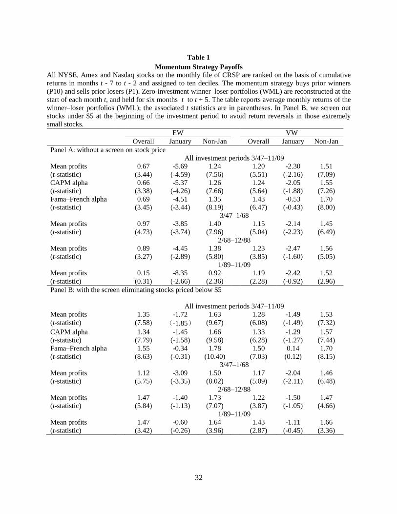
32

Table 1

Momentum Strategy Payoffs

All NYSE, Amex and Nasdaq stocks on the monthly file of CRSP are ranked on the basis of cumulative

returns in months t - 7 to t - 2 and assigned to ten deciles. The momentum strategy buys prior winners

(P10) and sells prior losers (P1). Zero-investment winner–loser portfolios (WML) are reconstructed at the

start of each month t, and held for six months t to t + 5. The table reports average monthly returns of the

winner–loser portfolios (WML); the associated t statistics are in parentheses. In Panel B, we screen out

stocks under $5 at the beginning of the investment period to avoid return reversals in those extremely

small stocks.

EW VW

Overall January Non-Jan Overall January Non-Jan

Panel A: without a screen on stock price

All investment periods 3/47–11/09

Mean profits 0.67 -5.69 1.24 1.20 -2.30 1.51

(t-statistic) (3.44) (-4.59) (7.56) (5.51) (-2.16) (7.09)

CAPM alpha 0.66 -5.37 1.26 1.24 -2.05 1.55

(t-statistic) (3.38) (-4.26) (7.66) (5.64) (-1.88) (7.26)

Fama–French alpha 0.69 -4.51 1.35 1.43 -0.53 1.70

(t-statistic) (3.45) (-3.44) (8.19) (6.47) (-0.43) (8.00)

3/47–1/68

Mean profits 0.97 -3.85 1.40 1.15 -2.14 1.45

(t-statistic) (4.73) (-3.74) (7.96) (5.04) (-2.23) (6.49)

2/68–12/88

Mean profits 0.89 -4.45 1.38 1.23 -2.47 1.56

(t-statistic) (3.27) (-2.89) (5.80) (3.85) (-1.60) (5.05)

1/89–11/09

Mean profits 0.15 -8.35 0.92 1.19 -2.42 1.52

(t-statistic) (0.31) (-2.66) (2.36) (2.28) (-0.92) (2.96)

Panel B: with the screen eliminating stocks priced below $5

All investment periods 3/47–11/09

Mean profits 1.35 -1.72 1.63 1.28 -1.49 1.53

(t-statistic) (7.58) （-1.85） (9.67) (6.08) (-1.49) (7.32)

CAPM alpha 1.34 -1.45 1.66 1.33 -1.29 1.57

(t-statistic) (7.79) (-1.58) (9.58) (6.28) (-1.27) (7.44)

Fama–French alpha 1.55 -0.34 1.78 1.50 0.14 1.70

(t-statistic) (8.63) (-0.31) (10.40) (7.03) (0.12) (8.15)

3/47–1/68

Mean profits 1.12 -3.09 1.50 1.17 -2.04 1.46

(t-statistic) (5.75) (-3.35) (8.02) (5.09) (-2.11) (6.48)

2/68–12/88

Mean profits 1.47 -1.40 1.73 1.22 -1.50 1.47

(t-statistic) (5.84) (-1.13) (7.07) (3.87) (-1.05) (4.66)

1/89–11/09

Mean profits 1.47 -0.60 1.64 1.43 -1.11 1.66

(t-statistic) (3.42) (-0.26) (3.96) (2.87) (-0.45) (3.36)

33

Table 2

Risk-premium estimates from two-stage Fama-MacBeth (1973) cross-sectional regressions: using

ten size-, ten value- and ten momentum portfolios as the base portfolios.

This table reports risk premiums of Chen, Roll and Ross (1986) five factors and Fama and French (1993)

three factors, including the growth rate of industrial production (MP), unexpected inflation (UI), change

in expected inflation (DEI), term premium (UTS), and default premium (UPR), market premium (MKT),

size premium (SMB) and value premium (HML) from two-stage Fama-MacBeth (1973) cross-sectional

regressions. The Fama-MacBeth t-statistics are calculated from the Shanken (1992) method and are

reported in parentheses, and the average cross-sectional are also reported. We use thirty base portfolios

that consist of decile one-sorted portfolios formed on size (market capitalization), value (book-to-market

equity) and momentum (past two-to-seven months’ returns). Note that the difference in the base portfolios

between Panels A and B is that Panel A includes ten equal-weighted decile momentum portfolios,

whereas Panel B consists of ten value-weighted decile momentum portfolios. In the first-stage time-series

regressions, for each test portfolio, we estimate factor loadings using the full samples, the extended

window and sixty-month rolling window regressions. In the second-stage cross-sectional regressions, we

estimate risk premiums by regressing base portfolios’ excess returns on factor loadings estimated from the

first-stage time-series regressions. We start the second-stage cross-sectional regressions from March 1949

in the entire sample of March 1947–November 2009, in order to ensure that there are at least two years of

monthly observations in the first-stage extended- and rolling-window time-series regressions. For the

extended-window case, the first-stage time-series regressions start from the first month to month t and the

second-stage cross-sectional regressions regress base portfolios’ excess returns in month t + 1 on factor

loadings using information up to month t. The table only reports the results based on the full samples in

the first-stage time-series regressions, and the extended-window regressions generate quantitatively

similar results. Panel A: Equal-Weighted Momentum Decile Portfolios

Overall

MP 0.45 1.07 12%

(2.83) (3.67)

FF 0.90 -0.25 0.17 0.17 43%

(3.44) (-0.83) (1.40) (1.58)

FF+MP 0.93 -0.22 0.09 0.21 1.07 49%

(3.53) (-0.74) (0.69) (1.95) (3.43)

CRR5 0.78 0.23 0.09 -1.22 0.25 0.76 46%

(4.48) (1.31) (0.50) (-2.57) (1.93) (2.68)

Non-January

MP 0.71 -0.34 20%

(4.38) (-1.04)

FF 1.42 -0.81 -0.11 0.04 42%

(5.73) (-2.72) (-0.82) (0.37)

FF+MP 1.45 -0.84 -0.13 0.05 0.16 45%

(5.95) (-2.82) (-0.99) (0.38) (0.43)

CRR5 1.20 0.35 0.10 -2.34 0.34 -0.03 46%

(6.56) (1.22) (0.29) (-5.72) (2.23) (-0.12)

Panel B: Value-Weighted Momentum Decile Portfolios

Overall

34

MP 0.35 1.24 12%

(2.05) (4.73)

FF 1.77 -1.13 0.19 0.13 39%

(5.32) (-2.96) (1.52) (1.02)

FF+MP 1.35 -0.62 0.02 0.21 1.41 49%

(4.59) (-1.89) (0.18) (1.81) (3.25)

CRR5 0.97 0.32 0.11 -1.83 0.22 0.80 41%

(5.52) (1.15) (0.36) (-3.05) (1.73) (2.88)

Non-January

MP 0.49 0.17 13%

(2.88) (0.62)

FF 2.03 -1.44 0.05 -0.02 38%

(6.29) (-3.75) (0.32) (-0.17)

FF+MP 1.94 -1.28 -0.07 -0.01 1.19 44%

(6.19) (-3.49) (-0.53) (-0.06) (2.01)

CRR5 1.34 0.44 0.12 -2.30 0.16 -0.19 39%

(7.40) (1.08) (0.26) (-5.68) (1.10) (-0.56)

35

Table 3

Risk-premium estimates from two-stage Fama–MacBeth (1973) cross-sectional regressions: using

10 size, 10 value, 10 momentum, and 10 industry portfolios as base portfolios

This table reports risk premiums of Chen, Roll, and Ross (1986) five factors and Fama and French (1993)

three factors, including the growth rate of industrial production (MP), unexpected inflation (UI), change

in expected inflation (DEI), term premium (UTS), and default premium (UPR), market premium (MKT),

size premium (SMB), and value premium (HML) estimated from two-stage Fama–MacBeth (1973) cross-

sectional regressions. The Fama–MacBeth t-statistics are calculated from the Shanken (1992) method and

are reported in parentheses and the average cross-sectional are also reported. We use forty base

portfolios that consist of ten size-, ten value-, ten momentum- and ten industry portfolios. Note that the

difference in the base portfolios between Panels A and B is that Panel A includes ten equal-weighted

decile momentum portfolios, whereas Panel B consists of ten value-weighted decile momentum portfolios.

In the first-stage time-series regressions, for each test portfolio, we estimate factor loadings using the full

samples, the extended window, and sixty-month rolling window regressions. In the second-stage cross-

sectional regressions, we estimate risk premiums by regressing base portfolios’ excess returns on factor

loadings estimated from the first-stage time-series regressions. We start the second-stage cross-sectional

regressions from March 1949 in the whole sample of March 1947–November 2009, in order to ensure that

there are at least two years of monthly observations in the first-stage extended-window time-series

regressions. For the extended-window case, the first-stage time-series regressions start from the first

month to month t and the second-stage cross-sectional regressions regress base portfolios’ excess returns

in month t + 1 on factor loadings using information from the first month to month t. The table only

reports the results based on the full samples in the first-stage time-series regressions, and the extended-

window regressions generate quantitatively similar results. Panel A: Equal-Weighted Momentum Decile Portfolios

Overall

MP 0.61 0.49 11%

(4.20) (2.31)

FF 0.66 0.00 0.17 0.09 38%

(3.43) (0.02) (1.46) (0.79)

FF+MP 0.99 -0.30 0.14 0.10 0.48 42%

(4.76) (-1.14) (1.16) (0.83) (2.28)

CRR5 0.79 0.18 0.08 -0.75 0.12 0.42 38%

(5.71) (0.86) (0.46) (-2.18) (1.23) (1.86)

Non-January

MP 0.66 -0.22 14%

(4.49) (-1.00)

FF 0.76 -0.16 -0.11 0.00 37%

(3.98) (-0.62) (-0.89) (0.01)

FF+MP 0.73 -0.13 -0.10 0.00 -0.05 40%

(3.99) (-0.52) (-0.86) (0.01) (-0.26)

CRR5 0.90 0.10 0.04 -1.75 0.02 0.53 38%

(6.14) (0.45) (0.18) (-5.73) (0.20) (2.35)

Panel B: Value-Weighted Momentum Decile Portfolios

Overall

36

MP 0.55 0.50 9%

(3.63) (2.72)

FF 1.04 -0.41 0.17 0.08 32%

(4.93) (-1.53) (1.45) (0.66)

FF+MP 1.42 -0.72 0.10 0.09 0.79 38%

(5.92) (-2.47) (0.83) (0.71) (2.76)

CRR5 0.86 0.19 0.08 -1.24 0.08 0.66 31%

(6.35) (0.81) (0.37) (-3.08) (0.83) (2.82)

Non-January

MP 0.58 -0.06 10%

(3.88) (-0.30)

FF 1.18 -0.61 0.02 -0.02 31%

(5.54) (-2.21) (0.18) (-0.19)

FF+MP 1.41 -0.80 -0.01 -0.04 0.44 36%

(6.19) (-2.78) (-0.11) (-0.28) (1.60)

CRR5 0.95 0.18 0.05 -1.53 -0.12 0.41 31%

(6.56) (0.73) (0.22) (-4.91) (-1.42) (1.84) (6.56)

37

Table 4

Expected momentum profits versus observed momentum profits (base portfolios: ten size-, value- and momentum portfolios)

This table reports estimated momentum profits based on four different factor models, including the one-factor MP model (MP), the Fama-French

(1993) model augmented with MP (FF+MP), the Chen, Roll and Ross (1986) model without the default premium (CRR4) and the Chen, Roll and

Ross (1986) model (CRR5). We calculate expected momentum profits as the sum of the products of factor sensitivities and estimated risk

premium: [ ] . Factor sensitivities ( ) are estimated from

. Risk premiums ( ) are estimated from two-stage Fama-MacBeth (1973) cross-sectional regressions using ten

size-, ten value- and ten momentum portfolios as base portfolios.21

In the first-stage time-series regressions, for each of thirty base portfolios, we

estimate factor sensitivities by regressing base portfolios’ returns on factors, using the full-sample, extended windows and rolling windows:

. In the second-stage cross-sectional regressions, we regress thirty base

portfolios’ excess returns on the estimated factor sensitivities from the first-stage time-series regressions for each month:

. This table also presents the t-statistics (e.g., t(diff1)) testing the null that the

difference between the observed momentum return and the incremental contribution of MP ( [ ]) is zero and the t-statistics (e.g., t(diff2))

testing the null that the difference between observed and expected momentum returns is zero.

[

]

[ ]

t(diff1) [ ] [ ]

t(diff2) [

]

[ ]

t(diff1) [ ] [ ]

t(diff2)

Panel A: equal-weighted momentum

Overall Non-January

Full-sample window in the first-stage regressions

MP 0.31 49% 1.44 0.31 49% 1.44 MP -0.01 — 7.12 -0.01 — 7.12

FF+MP 0.42 66% 1.69 0.36 56% 2.93 FF+MP 0.02 1% 7.15 0.08 7% 7.50

CRR4 0.24 39% 2.03 0.48 76% 2.81 CRR4 0.00 0% 7.13 0.95 80% 3.73

CRR5 0.14 23% 2.55 0.56 88% 1.84 CRR5 0.00 0% 7.14 1.05 88% 2.97

Extended window in the first-stage regressions

MP 0.14 22% 2.30 0.14 22% 2.30 MP 0.03 3% 7.05 0.03 3% 7.05

FF+MP 0.28 45% 2.19 0.20 31% 3.25 FF+MP 0.10 9% 6.92 0.20 17% 6.76

CRR4 0.08 13% 2.95 0.38 61% 3.27 CRR4 0.11 9% 6.90 0.60 50% 6.33

CRR5 0.03 5% 3.10 0.43 69% 3.30 CRR5 0.10 8% 6.91 0.72 60% 6.67

Rolling windows in the first-stage regressions

MP 0.08 13% 3.08 0.08 13% 3.08 MP 0.34 28% 5.39 0.34 28% 5.39

FF+MP 0.23 36% 2.89 0.17 27% 4.30 FF+MP 0.36 30% 5.88 0.48 40% 6.43

CRR4 0.12 19% 2.67 0.29 46% 3.30 CRR4 0.28 24% 5.66 0.58 49% 5.60

CRR5 0.09 14% 3.01 0.28 44% 3.92 CRR5 0.20 17% 6.21 0.64 53% 5.75

21 Please note that momentum portfolios used in Table 4–6 are constructed based on the sample of NYSE, AMEX and Nasdaq stocks on the CRSP monthly files. Momentum

portfolios utilized in Table 7 are constructed on the basis of the sample of NYSE and AMEX stocks on the CRSP monthly file as robustness check.

38

[

]

[ ]

t(diff1) [ ] [ ]

t(diff2) [

]

[ ]

t(diff1) [ ] [ ]

t(diff2)

Panel B: value-weighted momentum

Overall Non-January

Full-sample window in the first-stage regressions MP 0.41 34% 4.02 0.41 34% 4.02 MP 0.02 1% 6.86 0.02 1% 6.86

FF+MP 0.65 54% 4.43 0.67 55% 6.23 FF+MP 0.27 18% 7.07 0.49 32% 8.09

CRR4 0.21 18% 4.36 0.85 71% 4.51 CRR4 -0.02 — 6.74 1.13 75% 4.38

CRR5 0.15 13% 4.73 0.85 70% 4.55 CRR5 0.00 0% 6.87 1.14 76% 4.28

Extended window in the first-stage regressions

MP 0.18 15% 4.77 0.18 15% 4.77 MP 0.02 1% 6.76 0.02 1% 6.76

FF+MP 0.43 36% 4.98 0.42 35% 6.10 FF+MP 0.07 5% 6.85 0.17 11% 7.09

CRR4 0.24 20% 4.39 0.49 40% 5.89 CRR4 0.09 6% 6.65 0.39 26% 7.73

CRR5 0.16 13% 4.74 0.53 44% 5.74 CRR5 0.07 5% 6.76 0.47 31% 7.54

Rolling windows in the first-stage regressions

MP 0.18 15% 5.07 0.18 15% 5.07 MP 0.30 20% 6.26 0.30 20% 6.26

FF+MP 0.27 23% 5.23 0.39 32% 7.15 FF+MP 0.34 23% 6.00 0.61 40% 7.29

CRR4 0.21 18% 4.57 0.64 53% 5.06 CRR4 0.23 16% 6.37 0.77 51% 6.33

CRR5 0.13 11% 5.04 0.67 55% 5.61 CRR5 0.16 10% 6.79 0.88 58% 6.36

39

Table 5

Expected momentum profits versus observed momentum profits(base portfolios: ten size-, value-, momentum- and industry portfolios)

This table reports expected momentum returns based on four different factor models, including the one-factor MP model (MP), the Fama–French

(1993) model augmented with MP (FF+MP), the Chen Roll, and Ross (1986) model without default premium (CRR4) and the Chen, Roll, and

Ross (1986) model (CRR5). We calculate expected momentum returns as the sum of the products of factor sensitivities and estimated risk

premiums: [ ]

. Factor sensitivities ( ) are estimated from

. Risk premiums ( ) are estimated from two-stage Fama–MacBeth (1973) cross-sectional regressions, using ten

size-, ten value-, ten momentum- and ten industry portfolios as base portfolios. In the first-stage time-series regressions, for each of forty base

portfolios, we estimate factor sensitivities by regressing base portfolios’ returns on factors, using the full-sample, extended windows and rolling

windows:

. In the second-stage cross-sectional regressions, we regress

forty base portfolios’ excess returns on the estimated factor sensitivities from the first-stage time-series regressions for each month

. This table also presents the t-statistics (e.g., t(diff1)) testing the null that

the difference between the observed momentum return and the incremental contribution of MP ( [

]) is zero and the t-statistics (e.g., t(diff2))

testing the null that the difference between observed and expected momentum returns is zero.

[

]

[ ]

t(diff1) [ ] [ ]

t(diff2) [

]

[ ]

t(diff1) [ ] [ ]

t(diff2)

Panel A: equal-weighted momentum Overall Non-January

Full-sample window in the first-stage regressions MP 0.14 22% 2.21 0.14 22% 2.21 MP 0.00 0% 7.13 0.00 0% 7.13

FF+MP 0.19 30% 2.60 0.15 24% 3.24 FF+MP -0.01 0% 7.15 0.01 1% 7.48

CRR4 0.07 12% 2.96 0.35 56% 2.71 CRR4 0.01 1% 7.11 0.81 67% 3.43

CRR5 0.08 13% 2.93 0.43 68% 2.46 CRR5 -0.03 — 7.18 0.87 73% 3.38

Extended window in the first-stage regressions

MP 0.08 12% 2.63 0.08 12% 2.63 MP 0.03 3% 7.03 0.03 3% 7.03

FF+MP 0.04 7% 2.98 -0.04 — 3.75 FF+MP 0.05 4% 6.96 0.11 9% 6.75

CRR4 0.05 8% 2.98 0.36 56% 2.26 CRR4 0.06 5% 6.95 0.43 36% 5.72

CRR5 0.04 6% 3.11 0.40 63% 2.36 CRR5 0.05 4% 6.93 0.50 42% 5.80

Rolling window in the first-stage regressions

MP 0.01 2% 3.22 0.01 2% 3.22 MP 0.26 22% 5.71 0.26 22% 5.71

FF+MP 0.11 17% 3.31 0.05 7% 4.26 FF+MP 0.24 20% 6.17 0.32 27% 6.41

CRR4 0.07 11% 2.86 0.28 44% 2.41 CRR4 0.25 21% 5.77 0.51 43% 4.93

CRR5 0.08 13% 2.88 0.32 51% 2.26 CRR5 0.22 18% 6.10 0.57 48% 4.98

40

[ ] [ ]

t(diff1) [

] [ ]

t(diff2) [ ]

[ ]

t(diff1) [

] [ ]

t(diff2)

Panel B: value-weighted momentum Overall Non-January

Full-sample window in the first-stage regressions MP 0.16 14% 4.66 0.16 14% 4.66 MP -0.01 0% 6.84 -0.01 0% 6.84

FF+MP 0.37 30% 4.93 0.45 37% 5.74 FF+MP 0.10 7% 6.91 0.25 17% 7.66

CRR4 0.13 11% 4.89 0.69 58% 4.35 CRR4 0.03 2% 6.73 0.89 59% 4.60

CRR5 0.12 10% 4.99 0.71 59% 4.30 CRR5 -0.01 — 6.87 0.89 59% 4.64

Extended window in the first-stage regressions

MP 0.08 7% 4.96 0.08 7% 4.96 MP 0.02 1% 6.75 0.02 1% 6.75

FF+MP 0.14 11% 5.29 0.11 9% 5.88 FF+MP 0.01 1% 6.86 0.06 4% 6.89

CRR4 0.17 14% 4.59 0.39 32% 5.00 CRR4 0.05 3% 6.76 0.24 16% 7.18

CRR5 0.13 11% 4.85 0.44 37% 5.04 CRR5 0.03 2% 6.88 0.28 19% 7.25

Rolling window in the first-stage regressions

MP 0.10 8% 5.17 0.10 8% 5.17 MP 0.19 13% 6.4 0.19 13% 6.40

FF+MP 0.14 12% 5.52 0.20 17% 6.66 FF+MP 0.20 14% 6.36 0.39 26% 7.07

CRR4 0.17 14% 4.77 0.50 42% 4.76 CRR4 0.19 13% 6.35 0.62 41% 5.78

CRR5 0.11 9% 5.14 0.57 47% 4.88 CRR5 0.11 8% 6.76 0.71 47% 5.89

41

Table 6

Expected momentum returns versus observed momentum returns: using different industry portfolios as base portfolios

This table reports expected momentum returns based on four different factor models, including the one-factor MP model (MP), the Fama–French

(1993) model augmented with MP (FF+MP), the Chen, Roll and Ross (1986) model without the default premium (CRR4) and the Chen, Roll, and

Ross (1986) model (CRR5). We calculate expected momentum returns as the sum of the products of factor sensitivities and estimated risk

premiums: [ ]

. Factor sensitivities ( ) are estimated from

. Risk premiums ( ) are estimated from two-stage Fama–MacBeth (1973) cross-sectional regressions, using

different sets of base portfolios. In the first-stage time-series regressions, for each of the base portfolios, we estimate factor sensitivities by

regressing base portfolios’ returns on factors, using the full-sample, extended windows and rolling

windows:

. In the second-stage cross-sectional regressions, we regress the

base portfolios’ excess returns on the estimated factor sensitivities from the first-stage time-series regressions for each month

. This table also presents the t-statistics (e.g., t(diff1)) testing the null that the

difference between the observed momentum return and the incremental contribution of MP ( [

]) is zero and the t-statistics (e.g., t(diff2))

testing the null that the difference between observed and expected momentum returns is zero.

[

] [ ]

t(diff1) [ ]

[ ]

t(diff2) [

] [ ]

t(diff1) [ ]

[ ]

t(diff2)

Panel A: 10 size, 10 value, 10 momentum, and 17 industry portfolios as base portfolios

Overall Non-January

Full sample in the first-stage regressions

MP 0.11 17% 2.41 0.11 17% 2.41 MP -0.01 0% 7.14 -0.01 0% 7.14

FF+MP 0.16 25% 2.61 0.14 22% 3.07 FF+MP 0.00 0% 7.11 0.04 4% 7.22

CRR4 0.03 5% 3.01 0.20 32% 3.81 CRR4 0.00 0% 7.12 0.60 50% 4.64

CRR5 0.04 6% 3.04 0.24 37% 3.90 CRR5 -0.01 — 7.17 0.62 52% 4.75

Extended window in the first-stage regressions

MP 0.05 9% 2.75 0.05 9% 2.75 MP 0.03 2% 7.03 0.03 2% 7.03

FF+MP 0.04 6% 3.02 -0.06 — 3.80 FF+MP 0.03 2% 7.08 0.07 6% 6.90

CRR4 0.01 1% 3.13 0.21 33% 3.04 CRR4 0.05 4% 7.02 0.35 29% 5.94

CRR5 0.00 0% 3.21 0.26 42% 2.93 CRR5 0.05 4% 7.00 0.40 34% 5.84

Rolling window in the first-stage regressions

MP 0.14 22% 2.27 0.14 22% 2.27 MP 0.21 18% 5.95 0.21 18% 5.95

FF+MP 0.10 16% 2.47 0.04 6% 2.64 FF+MP 0.14 12% 6.54 0.22 18% 6.77

CRR4 0.14 21% 2.33 0.31 49% 1.33 CRR4 0.21 17% 6.05 0.47 39% 5.07

CRR5 0.15 23% 2.25 0.39 61% 1.01 CRR5 0.19 16% 6.17 0.52 44% 5.07

Panel B: 10 industry portfolios as base portfolios

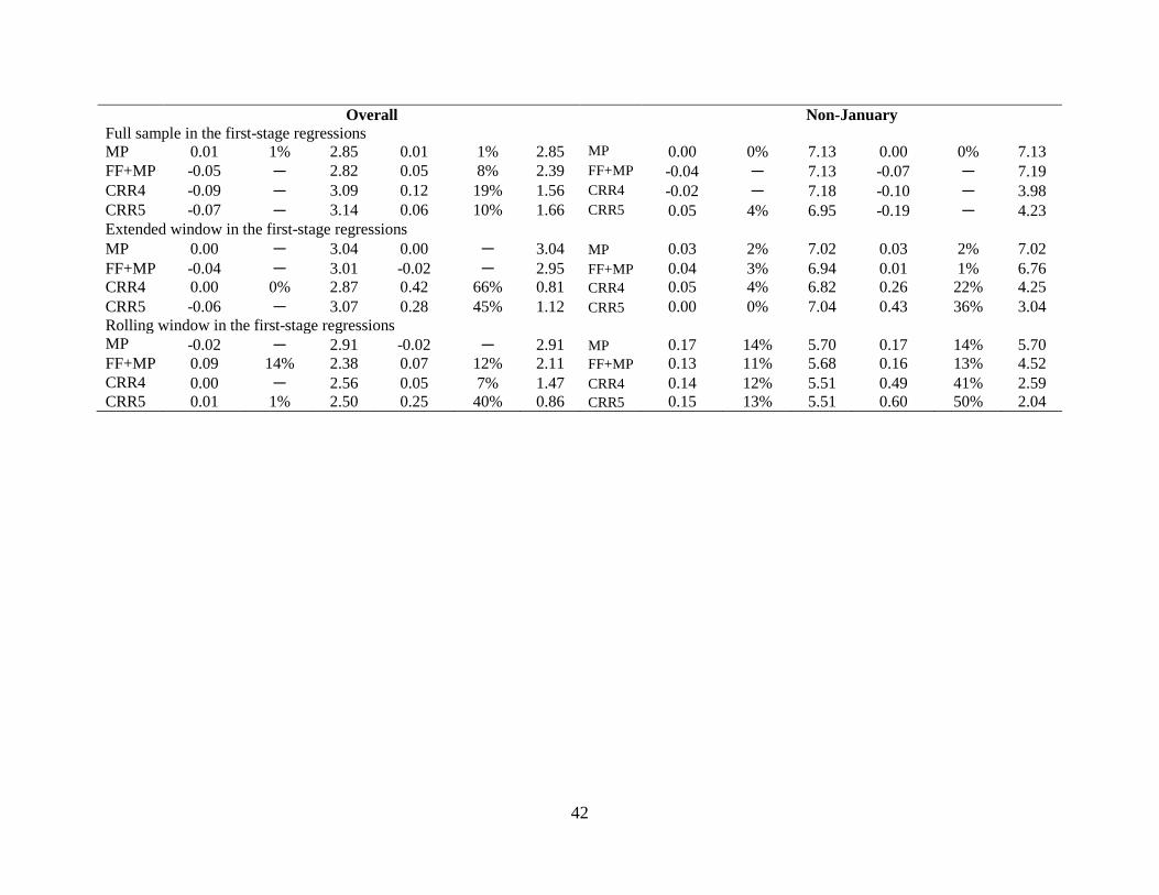
42

Overall Non-January

Full sample in the first-stage regressions

MP 0.01 1% 2.85 0.01 1% 2.85 MP 0.00 0% 7.13 0.00 0% 7.13

FF+MP -0.05 — 2.82 0.05 8% 2.39 FF+MP -0.04 — 7.13 -0.07 — 7.19

CRR4 -0.09 — 3.09 0.12 19% 1.56 CRR4 -0.02 — 7.18 -0.10 — 3.98

CRR5 -0.07 — 3.14 0.06 10% 1.66 CRR5 0.05 4% 6.95 -0.19 — 4.23

Extended window in the first-stage regressions

MP 0.00 — 3.04 0.00 — 3.04 MP 0.03 2% 7.02 0.03 2% 7.02

FF+MP -0.04 — 3.01 -0.02 — 2.95 FF+MP 0.04 3% 6.94 0.01 1% 6.76

CRR4 0.00 0% 2.87 0.42 66% 0.81 CRR4 0.05 4% 6.82 0.26 22% 4.25

CRR5 -0.06 — 3.07 0.28 45% 1.12 CRR5 0.00 0% 7.04 0.43 36% 3.04

Rolling window in the first-stage regressions

MP -0.02 — 2.91 -0.02 — 2.91 MP 0.17 14% 5.70 0.17 14% 5.70

FF+MP 0.09 14% 2.38 0.07 12% 2.11 FF+MP 0.13 11% 5.68 0.16 13% 4.52

CRR4 0.00 — 2.56 0.05 7% 1.47 CRR4 0.14 12% 5.51 0.49 41% 2.59

CRR5 0.01 1% 2.50 0.25 40% 0.86 CRR5 0.15 13% 5.51 0.60 50% 2.04

43

Table 7

Expected momentum profits versus observed NYSE-Amex momentum profits: using ten size-, ten value- and ten NYSE-Amex momentum

portfolios as base portfolios

This table reports expected momentum returns based on four different factor models, including the one-factor MP model (MP), the Fama–French

(1993) model augmented with MP (FF+MP), the Chen, Roll and Ross (1986) model without the default premium (CRR4) and the Chen, Roll, and

Ross (1986) model (CRR5). We calculate expected momentum returns as the sum of the products of factor sensitivities and estimated risk

premiums: [ ] . Factor sensitivities ( ) are estimated from

. Risk premiums ( ) are estimated from two-stage Fama–MacBeth (1973) cross-sectional

regressions, for the sample using ten size-, ten value- and ten NYSE–Amex momentum portfolios as base portfolios. In the first-stage time-series

regressions, for each of the thirty base portfolios, we estimate factor sensitivities by regressing base portfolios’ returns on factors, using the full-

sample and extended windows: . In the second-stage cross-sectional

regressions, we regress the thirty base portfolios’ excess returns on the estimated factor sensitivities from the first-stage time-series regressions

for each month: . This table also presents the t-statistics (e.g.,

t(diff1)) testing the null that the difference between the observed momentum return and the incremental contribution of MP ( [ ]) is zero

and the t-statistics (e.g., t(diff2)) testing the null that the difference between observed and expected momentum returns is zero.

[

]

[ ]

t(diff1) [ ] [ ]

t(diff2) [

]

[ ]

t(diff1) [ ] [ ]

t(diff2)

Panel A: equal-weighted momentum Overall Non-January

Full sample in the first-stage regressions

MP 0.38 48% 2.18 0.38 48% 2.18 MP 0.00 0% 7.07 0.00 0% 7.07

FF+MP 0.41 52% 3.23 0.31 40% 5.65 FF+MP 0.27 21% 7.74 0.38 30% 8.44

CRR4 0.19 24% 3.10 0.47 60% 4.69 CRR4 -0.01 -1% 7.45 0.95 74% 4.60

CRR5 0.17 22% 3.30 0.60 76% 3.46 CRR5 0.00 0% 7.48 1.09 85% 3.37

Extended window in the first-stage regressions

MP 0.12 15% 3.39 0.12 15% 3.39 MP 0.02 2% 7.23 0.02 2% 7.23

FF+MP 0.24 30% 4.00 0.13 17% 5.66 FF+MP 0.03 3% 7.67 0.10 8% 7.70

CRR4 0.07 9% 3.94 0.37 47% 4.75 CRR4 0.09 7% 7.06 0.58 46% 7.35

CRR5 0.02 3% 4.17 0.49 62% 4.30 CRR5 0.09 7% 7.17 0.74 58% 7.03

Rolling window in the first-stage regressions

MP 0.01 1% 4.74 0.01 1% 4.74 MP 0.20 16% 6.97 0.20 16% 6.97

FF+MP 0.24 30% 3.86 0.18 23% 5.75 FF+MP 0.24 19% 7.19 0.41 33% 7.49

CRR4 0.07 9% 3.93 0.37 47% 3.73 CRR4 0.16 12% 6.90 0.60 47% 6.19

CRR5 0.08 10% 3.91 0.36 46% 4.27 CRR5 0.13 10% 6.99 0.69 54% 6.10

Panel B: value-weighted momentum

44

Overall Non-January

Full sample in the first-stage regressions

MP 0.36 36% 3.57 0.36 36% 3.57 MP 0.02 2% 6.21 0.02 2% 6.21

FF+MP 0.51 51% 4.54 0.50 50% 6.03 FF+MP 0.23 18% 6.64 0.32 26% 7.33

CRR4 0.20 20% 3.94 0.61 61% 4.59 CRR4 -0.02 -2% 6.07 0.82 66% 4.69

CRR5 0.14 14% 4.36 0.59 59% 4.65 CRR5 0.00 0% 6.21 0.83 67% 4.62

Extended window in the first-stage regressions

MP 0.17 17% 4.39 0.17 17% 4.39 MP 0.02 1% 6.10 0.02 1% 6.10

FF+MP 0.35 35% 4.91 0.34 34% 5.96 FF+MP 0.05 4% 6.31 0.16 13% 6.17

CRR4 0.23 23% 4.04 0.48 48% 5.02 CRR4 0.07 6% 5.88 0.40 32% 6.03

CRR5 0.16 16% 4.45 0.51 51% 4.75 CRR5 0.06 5% 6.00 0.49 39% 5.74

Rolling window in the first-stage regressions

MP 0.16 16% 4.78 0.16 16% 4.78 MP 0.20 16% 5.90 0.20 16% 5.90

FF+MP 0.27 27% 4.50 0.33 33% 5.90 FF+MP 0.23 18% 5.81 0.48 39% 6.11

CRR4 0.18 18% 4.35 0.52 51% 4.57 CRR4 0.14 11% 6.04 0.65 52% 5.31

CRR5 0.14 14% 4.57 0.53 53% 5.01 CRR5 0.08 6% 6.30 0.71 57% 5.46

45

Figure 1 MP factor loadings of equal-weighted momentum portfolio returns

This figure presents the results from calendar-based time-series regressions on the growth rate of

industrial production (MP) using returns of ten equal-weighted momentum decile portfolios, L, P2,…,

P9,W, where L stands for losers and W denotes winners. The table below shows the MP loadings for ten

equal-weighted momentum deciles. The figure reports the MP factor loadings based on four different

factor models, including the one-factor MP model (MP), the Fama–French three-factor (1993) model

augmented with MP (FF+MP), the Chen, Roll and Ross (1986) model without default premium (CRR4)

and the Chen, Roll, and Ross (1986) model (CRR5). The Fama and French (1993) three factors consist of

the market factor (MKT), the value factor (HML) and the size factor (SMB). The Chen, Roll, and Ross

(1986) five factors include MP(the growth rate of industry production), UI (unexpected inflation), DEI

(change in expected inflation), UTS (term premium) and UPR (default premium).

Panel A:Overall

L P2 P3 P4 P5 P6 P7 P8 P9 W

MP 0.32 0.30 0.29 0.25 0.26 0.29 0.32 0.39 0.46 0.61

FF+MP -0.10 -0.09 -0.08 -0.10 -0.09 -0.04 -0.01 0.06 0.14 0.28

CRR4 0.23 0.25 0.25 0.22 0.22 0.26 0.28 0.34 0.40 0.52

CRR5 0.37 0.36 0.36 0.31 0.31 0.34 0.36 0.41 0.46 0.56

Panel B: Non-January

L P2 P3 P4 P5 P6 P7 P8 P9 W

MP 0.59 0.51 0.47 0.40 0.38 0.40 0.41 0.46 0.51 0.62

FF+MP 0.71 0.60 0.56 0.48 0.46 0.47 0.47 0.51 0.56 0.65

CRR4 0.68 0.56 0.51 0.44 0.42 0.44 0.45 0.50 0.57 0.70

CRR5 0.10 0.04 0.03 -0.03 -0.04 -0.01 0.00 0.05 0.10 0.20

-0.3-0.2-0.1

00.10.20.30.40.50.60.70.80.9

L P2 P3 P4 P5 P6 P7 P8 P9 W

MP

Lo

adin

gs

Panel A: Overall

MP FF+MP CRR4 CRR5

-0.3-0.2-0.1

00.10.20.30.40.50.60.70.80.9

L P2 P3 P4 P5 P6 P7 P8 P9 W

MP

Lo

adin

gs

Panel B: Non-January

MP FF+MP CRR4 CRR5

46

Figure 2

MP factor loadings of value-weighted momentum portfolio returns

This figure presents the results from calendar-based time-series regressions on the growth rate of

industrial production (MP) using returns of ten value-weighted momentum decile portfolios, L, P2,…,

P9,W, where L stands for losers and W denotes winners. The table below shows the MP loadings for ten

value-weighted momentum deciles. The figure reports the MP factor loadings based on four different

factor models, including the one-factor MP model (MP), the Fama–French three-factor (1993) model

augmented with MP (FF+MP), the Chen, Roll and Ross (1986) model without the default premium

(CRR4) and the Chen, Roll, and Ross (1986) model (CRR5). The Fama and French (1993) three factors

consist of the market factor (MKT), the value factor (HML) and the size factor (SMB). The Chen, Roll,

and Ross (1986) five factors include MP(the growth rate of industrial production), UI (unexpected

inflation), DEI (change in expected inflation), UTS (term premium) and UPR (default premium).

Panel A: Overall

L P2 P3 P4 P5 P6 P7 P8 P9 W

MP 0.14 0.13 0.13 0.10 0.09 0.13 0.21 0.30 0.36 0.47

FF+MP -0.25 -0.20 -0.18 -0.19 -0.19 -0.14 -0.06 0.04 0.11 0.21

CRR4 0.13 0.13 0.14 0.11 0.10 0.13 0.20 0.29 0.34 0.42

CRR5 0.23 0.20 0.21 0.17 0.15 0.18 0.24 0.32 0.35 0.42

Panel B: Non-January

L P2 P3 P4 P5 P6 P7 P8 P9 W

MP 0.40 0.21 0.23 0.05 0.02 0.02 0.13 0.22 0.24 0.42

FF+MP 0.06 -0.06 -0.01 -0.17 -0.20 -0.20 -0.09 -0.01 -0.02 0.12

CRR4 0.30 0.16 0.20 0.03 0.00 0.01 0.09 0.17 0.16 0.31

CRR5 0.44 0.30 0.36 0.16 0.11 0.13 0.20 0.29 0.28 0.41

-0.3-0.2-0.1

00.10.20.30.40.50.60.70.80.9

L P2 P3 P4 P5 P6 P7 P8 P9 W

MP

Lo

adin

gs

Panel A: Overall

MP FF+MP CRR4 CRR5

-0.3-0.2-0.10.00.10.20.30.40.50.60.70.80.9

L P2 P3 P4 P5 P6 P7 P8 P9 W

MP

Lo

adin

gs

Panel B: Non-January

MP FF+MP CRR4 CRR5

47

Figure 3

Event-time MP factor loadings on winners and losers

This figure presents the results from pooled time-series factor regressions on MP using returns of winners (W) and losers (L). For the all-month

regressions, the event month t + m (where m=0,1,…, 24) starts the month right after portfolio formation to the twenty-fourth month. For the non-

January regressions, the event month t + m (where m=0,1,…, 24) starts the month right after portfolio formation to the twenty-four month. For

each event month, we pool together across calendar month the observations of returns to winners and losers, the FF three factors (the market factor,

MKT; the value factor, HML; the size factor, SMB), and the CRR five factors (the growth rate of industrial production, MP; unexpected inflation,

UI; change in expected inflation, DEI; term premium, UTS; default premium, UPR) for each of event month t + m. We perform pooled time-series

factor regressions to estimate MP factor loadings for winners (solid line) and losers (broken line).

-0.5

-0.4

-0.3

-0.2

-0.1

0

0.1

0.2

0.3

0.4

0.5

0.6

0 3 6 9 1215182124

MP

Lo

adin

gs

Event Month

FF+MP: Overall

-0.3-0.2-0.1

00.10.20.30.40.50.60.70.80.9

1

0 3 6 9 1215182124

MP

Lo

adin

gs

Event Month

CRR4: Overall

0

0.1

0.2

0.3

0.4

0.5

0.6

0.7

0.8

0.9

1

1.1

0 3 6 9 1215182124

MP

Lo

adin

gs

Event Month

CRR5: Overall

-0.2-0.1

00.10.20.30.40.50.60.70.80.9

11.1

0 3 6 9 1215182124

MP

Lo

adin

gs

Event Month

MP: Overall

-0.2-0.1

00.10.20.30.40.50.60.70.80.9

11.1

0 3 6 9 1215182124

Mp

Lo

adin

gs

Event Month

MP: Non-January

0.2

0.3

0.4

0.5

0.6

0.7

0.8

0.9

1

1.1

0 3 6 9 1215182124

MP

Lo

adin

gs

Event Month

CRR5:Non-January

-0.5-0.4-0.3-0.2-0.1

00.10.20.30.40.50.6

0 3 6 9 1215182124

MP

Lo

adin

gs

Event Month

FF+MP:Non-January

-0.3-0.2-0.1

00.10.20.30.40.50.60.70.80.9

1

0 3 6 9 1215182124

MP

Lo

adin

gs

Event Month

CRR4:Non-January

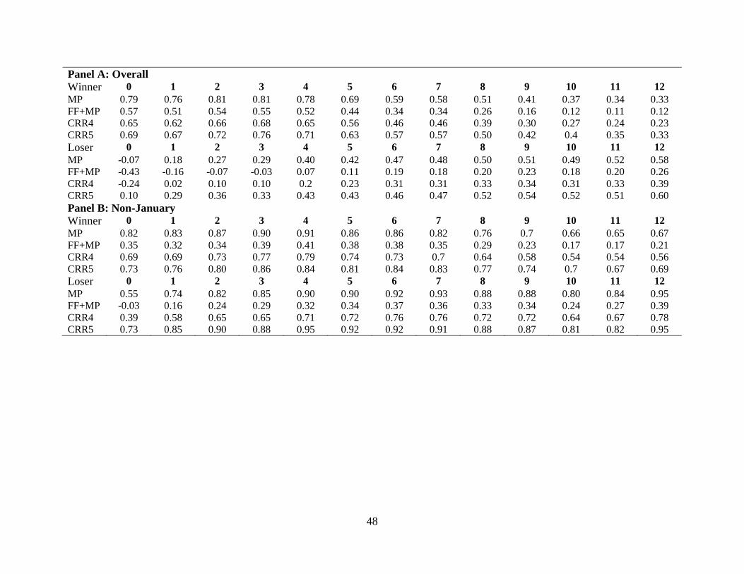
48

Panel A: Overall

Winner 0 1 2 3 4 5 6 7 8 9 10 11 12

MP 0.79 0.76 0.81 0.81 0.78 0.69 0.59 0.58 0.51 0.41 0.37 0.34 0.33

FF+MP 0.57 0.51 0.54 0.55 0.52 0.44 0.34 0.34 0.26 0.16 0.12 0.11 0.12

CRR4 0.65 0.62 0.66 0.68 0.65 0.56 0.46 0.46 0.39 0.30 0.27 0.24 0.23

CRR5 0.69 0.67 0.72 0.76 0.71 0.63 0.57 0.57 0.50 0.42 0.4 0.35 0.33

Loser 0 1 2 3 4 5 6 7 8 9 10 11 12

MP -0.07 0.18 0.27 0.29 0.40 0.42 0.47 0.48 0.50 0.51 0.49 0.52 0.58

FF+MP -0.43 -0.16 -0.07 -0.03 0.07 0.11 0.19 0.18 0.20 0.23 0.18 0.20 0.26

CRR4 -0.24 0.02 0.10 0.10 0.2 0.23 0.31 0.31 0.33 0.34 0.31 0.33 0.39

CRR5 0.10 0.29 0.36 0.33 0.43 0.43 0.46 0.47 0.52 0.54 0.52 0.51 0.60

Panel B: Non-January

Winner 0 1 2 3 4 5 6 7 8 9 10 11 12

MP 0.82 0.83 0.87 0.90 0.91 0.86 0.86 0.82 0.76 0.7 0.66 0.65 0.67

FF+MP 0.35 0.32 0.34 0.39 0.41 0.38 0.38 0.35 0.29 0.23 0.17 0.17 0.21

CRR4 0.69 0.69 0.73 0.77 0.79 0.74 0.73 0.7 0.64 0.58 0.54 0.54 0.56

CRR5 0.73 0.76 0.80 0.86 0.84 0.81 0.84 0.83 0.77 0.74 0.7 0.67 0.69

Loser 0 1 2 3 4 5 6 7 8 9 10 11 12

MP 0.55 0.74 0.82 0.85 0.90 0.90 0.92 0.93 0.88 0.88 0.80 0.84 0.95

FF+MP -0.03 0.16 0.24 0.29 0.32 0.34 0.37 0.36 0.33 0.34 0.24 0.27 0.39

CRR4 0.39 0.58 0.65 0.65 0.71 0.72 0.76 0.76 0.72 0.72 0.64 0.67 0.78

CRR5 0.73 0.85 0.90 0.88 0.95 0.92 0.92 0.91 0.88 0.87 0.81 0.82 0.95

49

Figure 4

The profitability of momentum strategies with respect to the Chen, Roll and Ross five-factor model

This table reports the value-weighted monthly returns to a total return momentum strategy (star ) as well as two alternative momentum strategies—

the factor-related return momentum strategy (solid line) and the stock-specific return momentum strategy(broken line). Each momentum strategy

assigns winners and losers as the top and bottom deciles of stocks by a ranking criterion. The ranking period is six months and the holding period

is six months, with one-month gap between ranking and holding. The factor-related return momentum strategy ranks stocks according to an

estimate of the factor component of their ranking period returns. The stock-specific return momentum strategy ranks stocks according to an

estimate of their component of their ranking period returns that is unrelated to macroeconomic risk factors. o distinguish the factor-related and

stock-specific components of their ranking period returns, We estimate the parameters of the Chen, Roll and Ross five-factor model for all of

NYSE, Amex and Nasdaq stocks i with minimum 36-month returns on the CRSP tapes, month t - 37 to t – 2: for max [t – 61], …, t – 2,

where the dummy of Dis equal to 1 if month is one of six ranking months; otherwise Dis equal to 0.

The stock-specific return momentum strategy ranks stocks by estimated i. The factor-related return momentum strategy ranks stocks based

on∑

. The total return momentum strategy and two alternative momentum

strategies are implemented in a comparable sample.

50

-37.18

-15.19

-40

-30

-20

-10

0

10

04/09 01/01 11/02 05/00 03/09 01/08 01/74 04/99 05/09 01/75

Pane A: Worst Monthly Momentum Returns

Overall

Stock-specific Factor-related Total

-37.18

-14.01

-40

-30

-20

-10

0

10

04/09 11/02 05/00 03/09 04/99 05/09 10/02 02/91 09/70 07/73

Panel B: Worst Monthly Momentum Returns

Non-January

Stock-specific Factor-related Total

12.85

35.84

-10

0

10

20

30

40

12/00 11/66 07/74 04/68 11/73 06/08 10/99 12/99 06/00 02/00

Panel C: Best Monthly Momentum Returns

Overall

Stock-specific Factor-related Total

12.85

35.84

-10

0

10

20

30

40

12/00 11/66 07/74 04/68 11/73 06/08 10/99 12/99 06/00 02/00

Panel D: Best Monthly Momentum Returns

Non-January

Stock-specific Factor-related Total