1

MOLECULAR SYMMETRY, GROUP THEORY, & APPLICATIONS Lecturer: Claire Vallance (CRL office G9, phone 75179, e-mail claire.vallance@chem.ox.ac.uk) These are the lecture notes for the second year general chemistry course named ‘Symmetry I’ in the course outline. They contain everything in the lecture slides, along with some additional information. You should, of course, feel free to make your own notes during the lectures if you want to as well. If anyone would desperately like a copy of the lecture slides, e-mail me at the end of the course and I’ll send you one (the file is about 2MB in size). At some point after each lecture and before the next, I STRONGLY recommend that you read the relevant sections of the lecture handout in order to consolidate the material from the previous lecture and refresh your memory. Most people (including me!) find group theory quite challenging the first time they encounter it, and you will probably find it difficult to absorb everything on the first go in the lectures without doing any additional reading. The good news is that a little extra effort on your part as we go along should easily prevent you from getting hopelessly lost! If you have questions at any point, please feel free to ask them either during or after the lectures, or contact me by e-mail or in the department (contact details above). Below is a (by no means comprehensive) list of some textbooks you may find useful for the course. If none of these appeal, have a look in your college library, the Hooke library or the RSL until you find one that suits you.

Atkins - Physical Chemistry Atkins - Molecular Quantum Mechanics Ogden – Introduction to Molecular Symmetry (Oxford Chemistry Primer) Cotton – Chemical Applications of Group Theory Davidson – Group Theory for Chemists Kettle – Symmetry and Structure Shriver, Atkins and Langford – Inorganic Chemistry Alan Vincent – Molecular Symmetry and Group Theory (Wiley)

Also, to get you started, here are a few useful websites. I’m sure there are many more, and if you find any others you think I should include, please e-mail me and let me know so I can alert future generations of second years. http://www.reciprocalnet.org/edumodules/symmetry/intro.html (a good tutorial on point groups and some aspects of symmetry and group theory, with lots of 3D molecular structures for you to play with) http://www.chemistry.nmsu.edu/studntres/chem639/symmetry/group.html (a helpful applet providing character tables and reduction of representations, which you’ll know all about by about lecture 5 of this course) NOTE: A PROBLEM SHEET IS ATTACHED TO THE END OF THIS HANDOUT

2

Contents 1. Introduction 2. Symmetry operations and symmetry elements 3. Symmetry classification of molecules – point groups 4. Symmetry and physical properties

4.1. Polarity 4.2. Chirality

5. Combining symmetry operations: ‘group multiplication’ 6. Constructing higher groups from simpler groups 7. Mathematical definition of a group 8. Review of Matrices

8.1. Definitions 8.2. Matrix algebra 8.3 Direct products 8.4. Inverse matrices and determinants

9. Transformation matrices 10. Matrix representations of groups

10.1. Example: a matrix representation of the C3v point group (the ammonia molecule) 10.2. Example: a matrix representation of the C2v point group (the allyl radical)

11. Properties of matrix representations 11.1. Similarity transforms 11.2. Characters of representations

12. Reduction of representations I 13. Irreducible representations and symmetry species 14. Character tables 15. Reduction of representations II

15.1 General concepts of orthogonality 15.2 Orthogonality relationships in group theory 15.3 Using the LOT to determine the irreps spanned by a basis

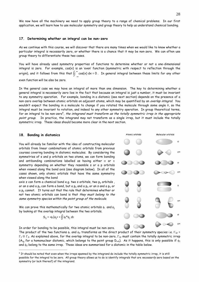
16. Symmetry adapted linear combinations 17. Determining whether an integral can be non-zero 18. Bonding in diatomics 19. Bonding in polyatomics - constructing molecular orbitals from SALCs 20. Calculating the orbital energies and expansion coefficients 21. Solving the secular equations

21.1 Matrix formulation of a set of linear equations 21.2 Solving for the orbital energies and expansion coefficients

22. Summary of the steps involved in constructing molecular orbitals 23. A more complicated bonding example – the molecular orbitals of H2O

23.1 Matrix representation, characters and SALCs 24. Molecular vibrations

24.1 Molecular degrees of freedom – determining the number of normal vibrational modes 24.2 Determining the symmetries of molecular motions 24.3 Atomic displacements using the 3N Cartesian basis 24.4 Molecular vibrations using internal coordinates

25. Summary of applying group theory to molecular motions 26. Group theory and molecular electronic states 27. Spectroscopy – interaction of atoms and molecules with light

27.1 Electronic transitions in molecules 27.2 Vibrational transitions in molecules 27.3 Raman scattering

28. Summary 29. Appendix A – a few proofs for the mathematically inclined 30. Appendix B – Character tables and direct product tables Problem sheet

3

1. Introduction You will already be familiar with the concept of symmetry in an everyday sense. If we say something is ‘symmetrical’, we usually mean it has mirror symmetry, or ‘left-right’ symmetry, and would look the same if viewed in a mirror. Symmetry is also very important in chemistry. Some molecules are clearly ‘more symmetrical’ than others, but what consequences does this have, if any? The aim of this course is to provide a systematic treatment of symmetry in chemical systems within the mathematical framework known as group theory (the reason for the name will become apparent later on). Once we have classified the symmetry of a molecule, group theory provides a powerful set of tools that provide us with considerable insight into many of its chemical and physical properties. Some applications of group theory that will be covered in this course include: i) Predicting whether a given molecule will be chiral, or polar.

ii) Examining chemical bonding and visualising molecular orbitals. iii) Predicting whether a molecule may absorb light of a given polarisation, and which spectroscopic transitions may be excited if it does. iv) Investigating the vibrational motions of the molecule.

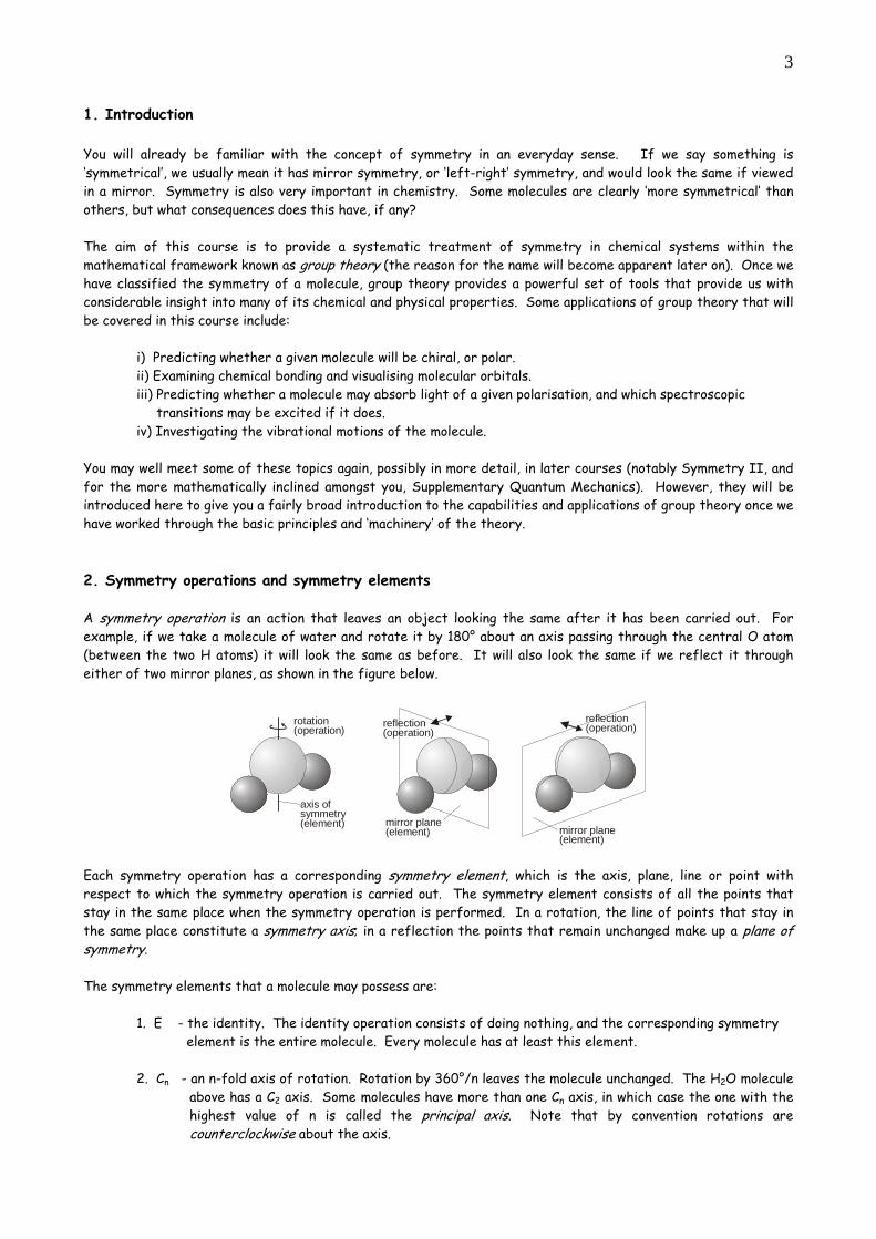
You may well meet some of these topics again, possibly in more detail, in later courses (notably Symmetry II, and for the more mathematically inclined amongst you, Supplementary Quantum Mechanics). However, they will be introduced here to give you a fairly broad introduction to the capabilities and applications of group theory once we have worked through the basic principles and ‘machinery’ of the theory. 2. Symmetry operations and symmetry elements A symmetry operation is an action that leaves an object looking the same after it has been carried out. For example, if we take a molecule of water and rotate it by 180° about an axis passing through the central O atom (between the two H atoms) it will look the same as before. It will also look the same if we reflect it through either of two mirror planes, as shown in the figure below.

rotation(operation)

axis of symmetry(element)

reflection(operation)

mirror plane(element)

reflection(operation)

mirror plane(element)

Each symmetry operation has a corresponding symmetry element, which is the axis, plane, line or point with respect to which the symmetry operation is carried out. The symmetry element consists of all the points that stay in the same place when the symmetry operation is performed. In a rotation, the line of points that stay in the same place constitute a symmetry axis; in a reflection the points that remain unchanged make up a plane of symmetry. The symmetry elements that a molecule may possess are: 1. E - the identity. The identity operation consists of doing nothing, and the corresponding symmetry element is the entire molecule. Every molecule has at least this element.

2. Cn - an n-fold axis of rotation. Rotation by 360°/n leaves the molecule unchanged. The H2O molecule above has a C2 axis. Some molecules have more than one Cn axis, in which case the one with the highest value of n is called the principal axis. Note that by convention rotations are counterclockwise about the axis.

4

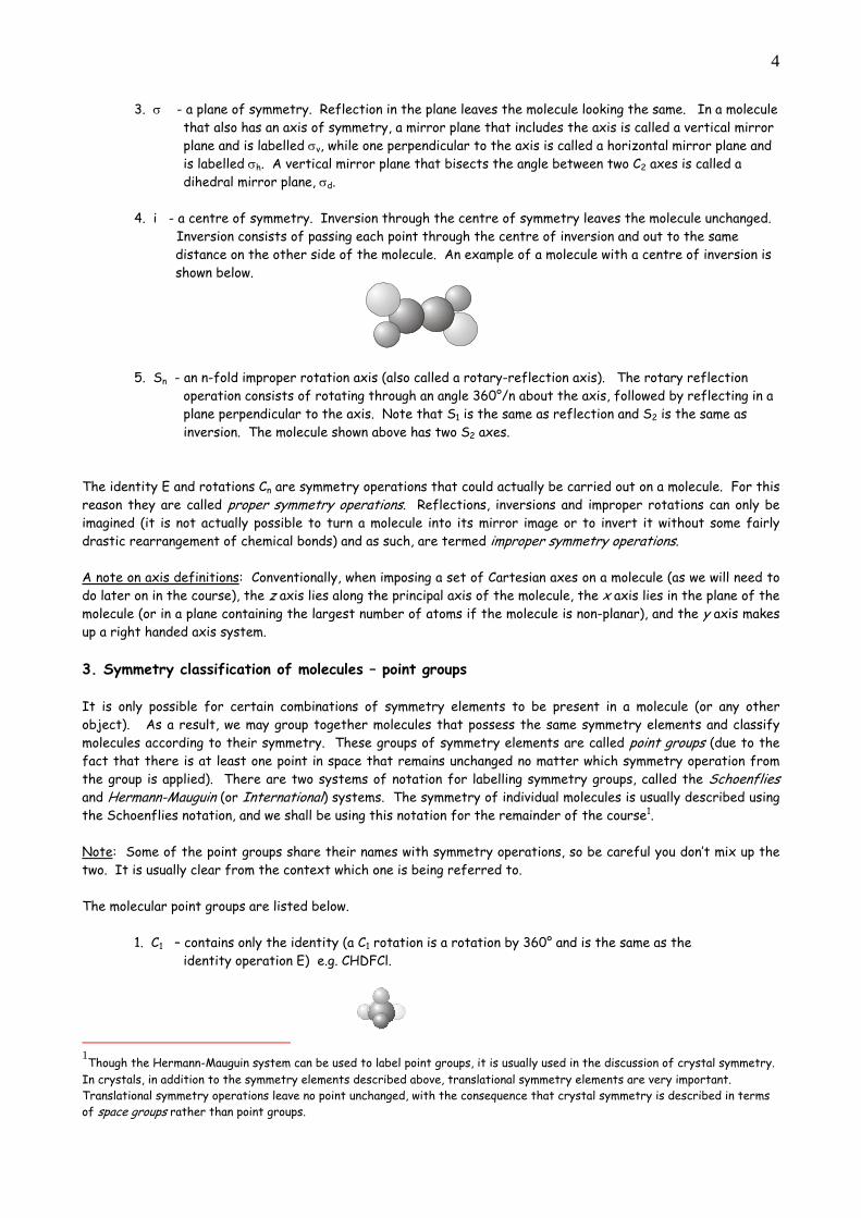
3. σ - a plane of symmetry. Reflection in the plane leaves the molecule looking the same. In a molecule that also has an axis of symmetry, a mirror plane that includes the axis is called a vertical mirror plane and is labelled σv, while one perpendicular to the axis is called a horizontal mirror plane and is labelled σh. A vertical mirror plane that bisects the angle between two C2 axes is called a dihedral mirror plane, σd. 4. i - a centre of symmetry. Inversion through the centre of symmetry leaves the molecule unchanged.

Inversion consists of passing each point through the centre of inversion and out to the same distance on the other side of the molecule. An example of a molecule with a centre of inversion is shown below.

5. Sn - an n-fold improper rotation axis (also called a rotary-reflection axis). The rotary reflection operation consists of rotating through an angle 360°/n about the axis, followed by reflecting in a plane perpendicular to the axis. Note that S1 is the same as reflection and S2 is the same as inversion. The molecule shown above has two S2 axes.

The identity E and rotations Cn are symmetry operations that could actually be carried out on a molecule. For this reason they are called proper symmetry operations. Reflections, inversions and improper rotations can only be imagined (it is not actually possible to turn a molecule into its mirror image or to invert it without some fairly drastic rearrangement of chemical bonds) and as such, are termed improper symmetry operations. A note on axis definitions: Conventionally, when imposing a set of Cartesian axes on a molecule (as we will need to do later on in the course), the z axis lies along the principal axis of the molecule, the x axis lies in the plane of the molecule (or in a plane containing the largest number of atoms if the molecule is non-planar), and the y axis makes up a right handed axis system. 3. Symmetry classification of molecules – point groups It is only possible for certain combinations of symmetry elements to be present in a molecule (or any other object). As a result, we may group together molecules that possess the same symmetry elements and classify molecules according to their symmetry. These groups of symmetry elements are called point groups (due to the fact that there is at least one point in space that remains unchanged no matter which symmetry operation from the group is applied). There are two systems of notation for labelling symmetry groups, called the Schoenflies and Hermann-Mauguin (or International) systems. The symmetry of individual molecules is usually described using the Schoenflies notation, and we shall be using this notation for the remainder of the course1. Note: Some of the point groups share their names with symmetry operations, so be careful you don’t mix up the two. It is usually clear from the context which one is being referred to. The molecular point groups are listed below. 1. C1 – contains only the identity (a C1 rotation is a rotation by 360° and is the same as the identity operation E) e.g. CHDFCl.

1Though the Hermann-Mauguin system can be used to label point groups, it is usually used in the discussion of crystal symmetry. In crystals, in addition to the symmetry elements described above, translational symmetry elements are very important. Translational symmetry operations leave no point unchanged, with the consequence that crystal symmetry is described in terms of space groups rather than point groups.

5

2. Ci - contains the identity E and a centre of inversion i.

3. CS - contains the identity E and a plane of reflection σ.

4. Cn – contains the identity and an n-fold axis of rotation.

5. Cnv – contains the identity, an n-fold axis of rotation, and n vertical mirror planes σv.

6. Cnh - contains the identity, an n-fold axis of rotation, and a horizontal reflection plane σh (note that in C2h this combination of symmetry elements automatically implies a centre of inversion).

7. Dn - contains the identity, an n-fold axis of rotation, and n 2-fold rotations about axes perpendicular to the principal axis. 8. Dnh - contains the same symmetry elements as Dn with the addition of a horizontal mirror plane.

9. Dnd - contains the same symmetry elements as Dn with the addition of n dihedral mirror planes.

10. Sn - contains the identity and one Sn axis. Note that molecules only belong to Sn if they have not already been classified in terms of one of the preceding point groups (e.g. S2 is the same as Ci, and a molecule with this symmetry would already have been classified). The following groups are the cubic groups, which contain more than one principal axis. They separate into the tetrahedral groups (Td, Th and T) and the octahedral groups (O and Oh). The icosahedral group also exists but is not included below.

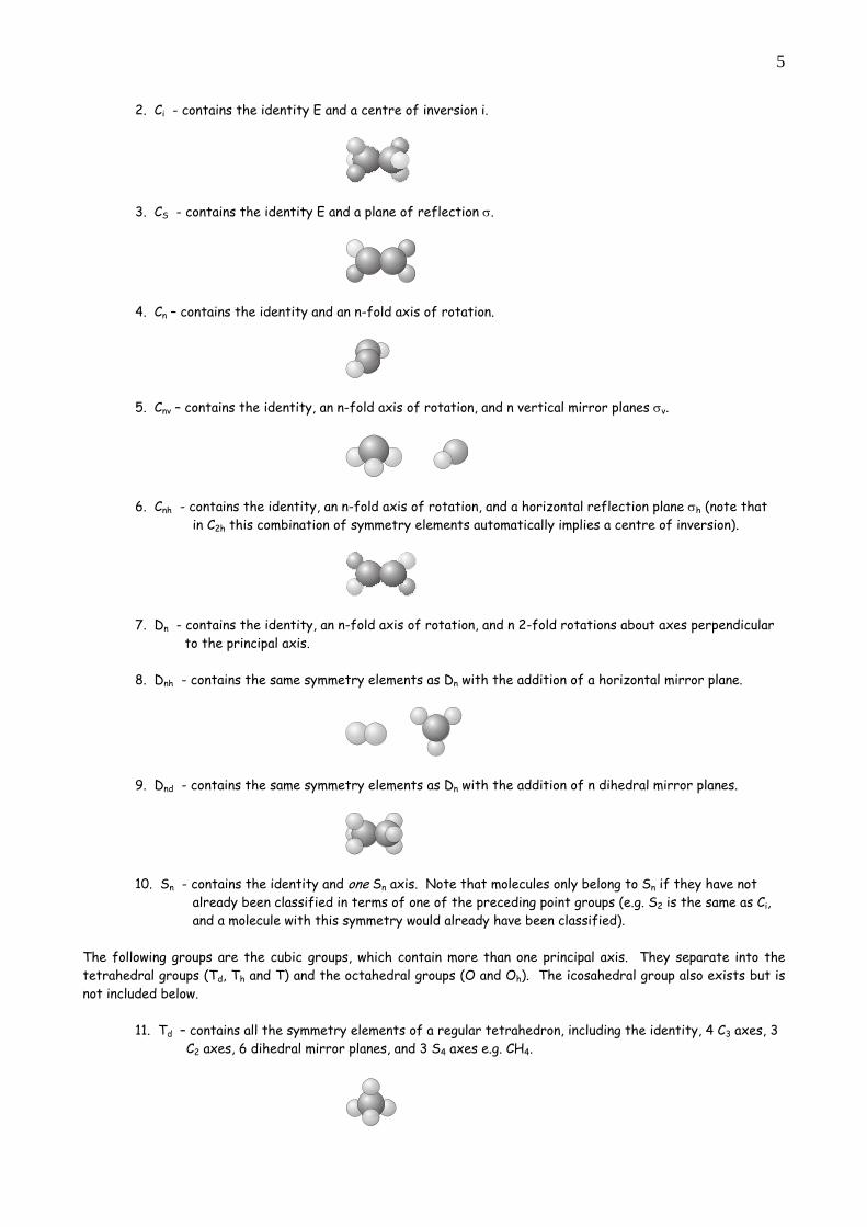
11. Td – contains all the symmetry elements of a regular tetrahedron, including the identity, 4 C3 axes, 3 C2 axes, 6 dihedral mirror planes, and 3 S4 axes e.g. CH4.

6

12. T - as for Td but no planes of reflection.

13. Th – as for T but contains a centre of inversion. 14. Oh – the group of the regular octahedron e.g. SF6.

15. O - as for Oh but with no planes of reflection. The final group is the full rotation group R3, which consists of an infinite number of Cn axes with all possible values of n and describes the symmetry of a sphere. Atoms (but no molecules) belong to R3, and the group has important applications in atomic quantum mechanics. However, we won’t be treating it any further here. Once you become more familiar with the symmetry elements and point groups described above, you will find it quite straightforward to classify a molecule in terms of its point group. In the meantime, the flowchart shown below provides a step-by-step approach to the problem.

Is the molecule linear?

Does it have a centreof inversion?

Does it have two or moreC axes with n>2?n

Does it have a C axis?n

D h∞

C v∞

Y

Y

Y

N

N

Y

Does it have a centreof inversion?

Td

Does it have aC axis?5

Ih

Oh

Y

Y

N

N

START

Does it have a mirror plane?

Cs

Does it have a centreof inversion?

C1

Ci

N

Y

Y

N

N

Are there n C axesperpendicular to theprincipal axis?

2

Is there a horizontalmirror plane?

Is there a horizontalmirror plane?

Dnh

Are there n dihedralmirror planes?

Are there n verticalmirror planes?

Dnd

Dn

Cnh

Cnv

Y

N

N

N

N

Is there an Saxis?

2nS2n

Cn

7

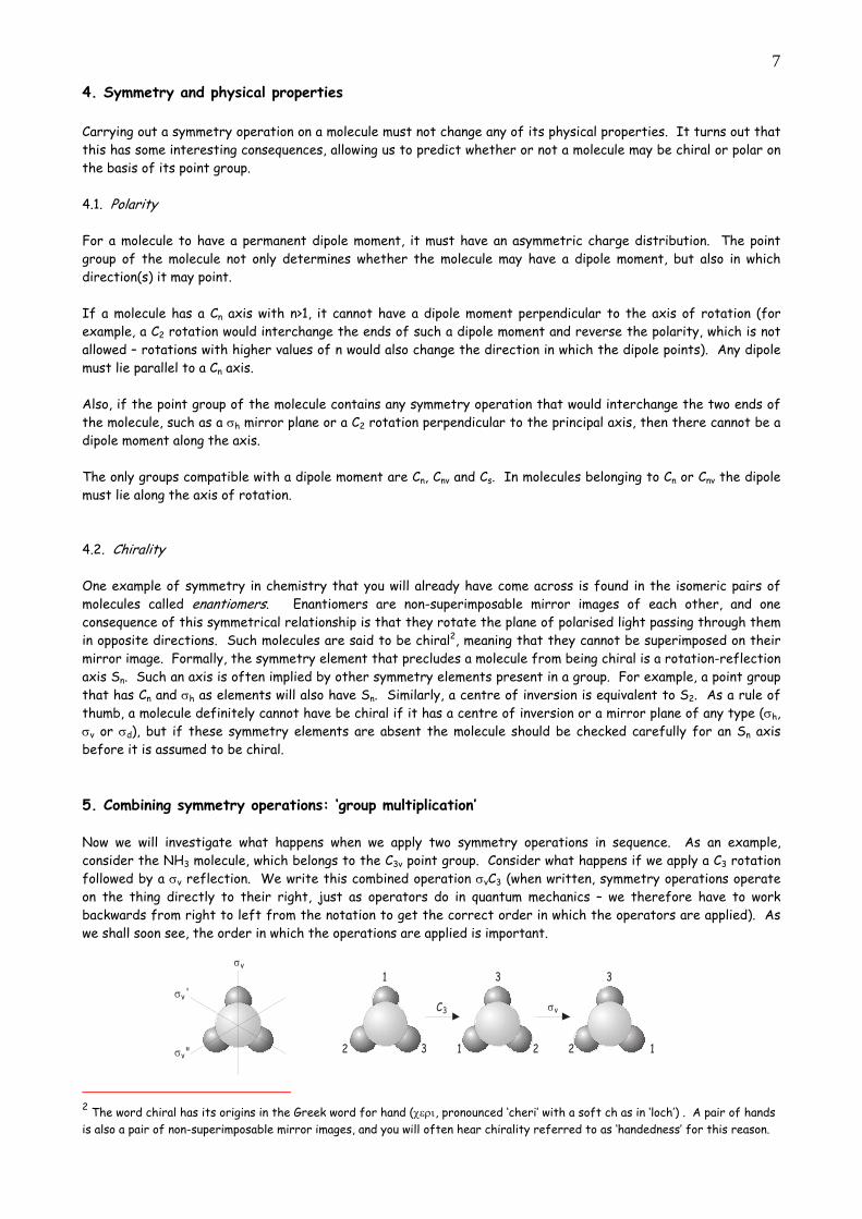
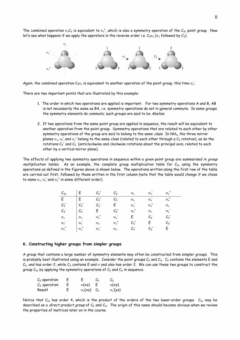
4. Symmetry and physical properties Carrying out a symmetry operation on a molecule must not change any of its physical properties. It turns out that this has some interesting consequences, allowing us to predict whether or not a molecule may be chiral or polar on the basis of its point group. 4.1. Polarity For a molecule to have a permanent dipole moment, it must have an asymmetric charge distribution. The point group of the molecule not only determines whether the molecule may have a dipole moment, but also in which direction(s) it may point. If a molecule has a Cn axis with n>1, it cannot have a dipole moment perpendicular to the axis of rotation (for example, a C2 rotation would interchange the ends of such a dipole moment and reverse the polarity, which is not allowed – rotations with higher values of n would also change the direction in which the dipole points). Any dipole must lie parallel to a Cn axis. Also, if the point group of the molecule contains any symmetry operation that would interchange the two ends of the molecule, such as a σh mirror plane or a C2 rotation perpendicular to the principal axis, then there cannot be a dipole moment along the axis. The only groups compatible with a dipole moment are Cn, Cnv and Cs. In molecules belonging to Cn or Cnv the dipole must lie along the axis of rotation. 4.2. Chirality One example of symmetry in chemistry that you will already have come across is found in the isomeric pairs of molecules called enantiomers. Enantiomers are non-superimposable mirror images of each other, and one consequence of this symmetrical relationship is that they rotate the plane of polarised light passing through them in opposite directions. Such molecules are said to be chiral2, meaning that they cannot be superimposed on their mirror image. Formally, the symmetry element that precludes a molecule from being chiral is a rotation-reflection axis Sn. Such an axis is often implied by other symmetry elements present in a group. For example, a point group that has Cn and σh as elements will also have Sn. Similarly, a centre of inversion is equivalent to S2. As a rule of thumb, a molecule definitely cannot have be chiral if it has a centre of inversion or a mirror plane of any type (σh, σv or σd), but if these symmetry elements are absent the molecule should be checked carefully for an Sn axis before it is assumed to be chiral. 5. Combining symmetry operations: ‘group multiplication’ Now we will investigate what happens when we apply two symmetry operations in sequence. As an example, consider the NH3 molecule, which belongs to the C3v point group. Consider what happens if we apply a C3 rotation followed by a σv reflection. We write this combined operation σvC3 (when written, symmetry operations operate on the thing directly to their right, just as operators do in quantum mechanics – we therefore have to work backwards from right to left from the notation to get the correct order in which the operators are applied). As we shall soon see, the order in which the operations are applied is important.

1

112 2 23

33

σv

σv

σv'

σv"

C3

2 The word chiral has its origins in the Greek word for hand (χερι, pronounced ‘cheri’ with a soft ch as in ‘loch’) . A pair of hands is also a pair of non-superimposable mirror images, and you will often hear chirality referred to as ‘handedness’ for this reason.

8

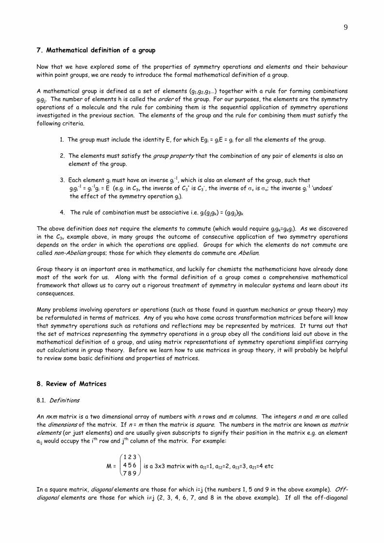
The combined operation σvC3 is equivalent to σv’’, which is also a symmetry operation of the C3v point group. Now let’s see what happens if we apply the operators in the reverse order i.e. C3σv (σv followed by C3).

1

1

1

2 2

2

3 33

σv

σv C3

σv'

σv"

Again, the combined operation C3σv is equivalent to another operation of the point group, this time σv’. There are two important points that are illustrated by this example:

1. The order in which two operations are applied is important. For two symmetry operations A and B, AB is not necessarily the same as BA, i.e. symmetry operations do not in general commute. In some groups the symmetry elements do commute; such groups are said to be Abelian. 2. If two operations from the same point group are applied in sequence, the result will be equivalent to another operation from the point group. Symmetry operations that are related to each other by other symmetry operations of the group are said to belong to the same class. In NH3, the three mirror planes σv, σv’ and σv’’ belong to the same class (related to each other through a C3 rotation), as do the rotations C3

+ and C3- (anticlockwise and clockwise rotations about the principal axis, related to each

other by a vertical mirror plane). The effects of applying two symmetry operations in sequence within a given point group are summarised in group multiplication tables. As an example, the complete group multiplication table for C3v using the symmetry operations as defined in the figures above is shown below. The operations written along the first row of the table are carried out first, followed by those written in the first column (note that the table would change if we chose to name σv, σv’ and σv’’ in some different order). 6. Constructing higher groups from simpler groups A group that contains a large number of symmetry elements may often be constructed from simpler groups. This is probably best illustrated using an example. Consider the point groups C2 and CS. C2 contains the elements E and C2, and has order 2, while CS contains E and σ and also has order 2. We can use these two groups to construct the group C2v by applying the symmetry operations of C2 and CS in sequence.

C2 operation E E C2 C2 CS operation E σ(xz) E σ(xz) Result E σv(xz) C2 σv’(yz)

Notice that C2v has order 4, which is the product of the orders of the two lower-order groups. C2v may be described as a direct product group of C2 and CS. The origin of this name should become obvious when we review the properties of matrices later on in the course.

C3v E C3+ C3

- σv σv’ σv’’ E E C3

+ C3- σv σv’ σv’’

C3+ C3

+ C3- E σv’ σv’’ σv

C3- C3

- E C3+ σv’’ σv σv’

σv σv σv’’ σv’ E C3- C3

+ σv’ σv’ σv σv’’ C3

+ E C3-

σv’’ σv’’ σv’ σv C3- C3

+ E

9

7. Mathematical definition of a group Now that we have explored some of the properties of symmetry operations and elements and their behaviour within point groups, we are ready to introduce the formal mathematical definition of a group. A mathematical group is defined as a set of elements (g1,g2,g3…) together with a rule for forming combinations gigj. The number of elements h is called the order of the group. For our purposes, the elements are the symmetry operations of a molecule and the rule for combining them is the sequential application of symmetry operations investigated in the previous section. The elements of the group and the rule for combining them must satisfy the following criteria. 1. The group must include the identity E, for which Egi = giE = gi for all the elements of the group.

2. The elements must satisfy the group property that the combination of any pair of elements is also an element of the group.

3. Each element gi must have an inverse gi

-1, which is also an element of the group, such that gigi

-1 = gi-1gi = E (e.g. in C3v the inverse of C3

+ is C3-, the inverse of σv is σv; the inverse gi

-1 ‘undoes’ the effect of the symmetry operation gi). 4. The rule of combination must be associative i.e. gi(gjgk) = (gigj)gk

The above definition does not require the elements to commute (which would require gigk=gkgi). As we discovered in the C3v example above, in many groups the outcome of consecutive application of two symmetry operations depends on the order in which the operations are applied. Groups for which the elements do not commute are called non-Abelian groups; those for which they elements do commute are Abelian. Group theory is an important area in mathematics, and luckily for chemists the mathematicians have already done most of the work for us. Along with the formal definition of a group comes a comprehensive mathematical framework that allows us to carry out a rigorous treatment of symmetry in molecular systems and learn about its consequences. Many problems involving operators or operations (such as those found in quantum mechanics or group theory) may be reformulated in terms of matrices. Any of you who have come across transformation matrices before will know that symmetry operations such as rotations and reflections may be represented by matrices. It turns out that the set of matrices representing the symmetry operations in a group obey all the conditions laid out above in the mathematical definition of a group, and using matrix representations of symmetry operations simplifies carrying out calculations in group theory. Before we learn how to use matrices in group theory, it will probably be helpful to review some basic definitions and properties of matrices. 8. Review of Matrices 8.1. Definitions An nxm matrix is a two dimensional array of numbers with n rows and m columns. The integers n and m are called the dimensions of the matrix. If n = m then the matrix is square. The numbers in the matrix are known as matrix elements (or just elements) and are usually given subscripts to signify their position in the matrix e.g. an element aij would occupy the ith row and jth column of the matrix. For example:

M = ⎝⎜⎛

⎠⎟⎞1 2 3

4 5 67 8 9

is a 3x3 matrix with a11=1, a12=2, a13=3, a21=4 etc

In a square matrix, diagonal elements are those for which i=j (the numbers 1, 5 and 9 in the above example). Off-diagonal elements are those for which i≠j (2, 3, 4, 6, 7, and 8 in the above example). If all the off-diagonal

10

elements are equal to zero then we have a diagonal matrix. We will see later that diagonal matrices are of considerable importance in group theory. A unit matrix or identity matrix (usually given the symbol I) is a diagonal matrix in which all the diagonal elements are equal to 1. A unit matrix acting on another matrix has no effect – it is the same as the identity operation in group theory and is analogous to multiplying a number by 1 in everyday arithmetic. The transpose AT of a matrix A is the matrix that results from interchanging all the rows and columns. A symmetric matrix is the same as its transpose (AT=A i.e. aij=aji for all values of i and j). The transpose of matrix M above (which is not symmetric) is

MT = ⎝⎜⎛

⎠⎟⎞1 4 7

2 5 83 6 9

The sum of the diagonal elements in a square matrix is called the trace (or character) of the matrix (for the above matrix, the trace is χ = 1 + 5 + 9 = 15). The traces of matrices representing symmetry operations will turn out to be of great importance in group theory. A vector is just a special case of a matrix in which one of the dimensions is equal to 1. An nx1 matrix is a column vector; a 1xm matrix is a row vector. The components of a vector are usually only labelled with one index. A unit vector has one element equal to 1 and the others equal to zero (it is the same as one row or column of an identity matrix). We can extend the idea further to say that a single number is a matrix (or vector) of dimension 1x1. 8.2. Matrix algebra i) Two matrices with the same dimensions may be added or subtracted by adding or subtracting the elements occupying the same position in each matrix. e.g.

A = ⎝⎜⎛

⎠⎟⎞1 0 2

2 2 13 2 0

B = ⎝⎜⎛

⎠⎟⎞2 0 -2

1 0 11 -1 0

A + B = ⎝⎜⎛

⎠⎟⎞3 0 0

3 2 24 1 0

A – B = ⎝⎜⎛

⎠⎟⎞-1 0 4

1 2 02 3 0

ii) A matrix may be multiplied by a constant by multiplying each element by the constant.

4B = ⎝⎜⎛

⎠⎟⎞8 0 -8

4 0 44 -4 0

3A = ⎝⎜⎛

⎠⎟⎞3 0 6

6 6 39 6 0

iii) Two matrices may be multiplied together provided that the number of columns of the first matrix is the same as the number of rows of the second matrix i.e. an nxm matrix may be multiplied by an mxl matrix. The resulting matrix will have dimensions nxl. To find the element aij in the product matrix, we take the dot product of row i of the first matrix and column j of the second matrix (i.e. we multiply consecutive elements together from row i of the first matrix and column j of the second matrix and add them together i.e. cij = Σk aikbkj e.g. in the 3x3 matrices A and B used in the above examples, the first element in the product matrix C = AB is c11=a11b11+a12b21+a13b31

AB = ⎝⎜⎛

⎠⎟⎞1 0 2

2 2 13 2 0 ⎝

⎜⎛

⎠⎟⎞2 0 -2

1 0 11 -1 0

= ⎝⎜⎛

⎠⎟⎞4 -2 -2

7 -1 -28 0 -4

An example of a matrix multiplying a vector is

Av = ⎝⎜⎛

⎠⎟⎞1 0 2

2 2 13 2 0 ⎝

⎜⎛

⎠⎟⎞1

23

= ⎝⎜⎛

⎠⎟⎞7

97

11

Matrix multiplication is not generally commutative, a property that mirrors the behaviour found earlier for symmetry operations within a point group.

8.3 Direct products The direct product of two matrices (given the symbol ⊗) is a special type of matrix product that generates a matrix of higher dimensionality if both matrices have dimension greater than one. The easiest way to demonstrate how to construct a direct product of two matrices A and B is by an example:

A ⊗ B = ⎝⎛

⎠⎞a11 a12

a21 a22 ⊗ ⎝

⎛⎠⎞b11 b12

b21 b22

= ⎝⎛

⎠⎞a11B a12B

a21B a22B

=

⎝⎜⎛

⎠⎟⎞a11b11 a11b12 a12b11 a11b12

a11b21 a11b22 a12b21 a12b22

a21b11 a21b12 a22b11 a22b12

a21b21 a21b22 a22b21 a22b22

Though this may seem like a somewhat strange operation to carry out, direct products crop up a great deal in group theory. 8.4. Inverse matrices and determinants If two square matrices A and B multiply together to give the identity matrix I (i.e. AB = I) then B is said to be the inverse of A (written A-1). If B is the inverse of A then A is also the inverse of B. Recall that one of the conditions imposed upon the symmetry operations in a group is that each operation must have an inverse. It follows by analogy that any matrices we use to represent symmetry elements must also have inverses. It turns out that a square matrix only has an inverse if its determinant is non-zero. For this reason (and others which will become apparent later on when we need to solve equations involving matrices) we need to learn a little about matrix determinants and their properties. For every square matrix, there is a unique function of all the elements that yields a single number called the determinant. Initially it probably won’t be particularly obvious why this number should be useful, but matrix determinants are of great importance both in pure mathematics and in a number of areas of science. Historically, determinants were actually around before matrices. They arose originally as a property of a system of linear equations that ‘determined’ whether the system had a unique solution. As we shall see later, when such a system of equations is recast as a matrix equation this property carries over into the matrix determinant. There are two different definitions of a determinant, one geometric and one algebraic. In the geometric interpretation, we consider the numbers across each row of an nxn matrix as coordinates in n-dimensional space. In a one-dimensional matrix (i.e. a number), there is only one coordinate, and the determinant can be interpreted as the (signed) length of a vector from the origin to this point. For a 2x2 matrix we have two coordinates in a plane, and the determinant is the (signed) area of the parallelogram that includes these two points and the origin. For a 3x3 matrix the determinant is the (signed) volume of the parallelepiped that includes the three points (in three-dimensional space) defined by the matrix and the origin. This is illustrated below. The idea extends up to higher dimensions in a similar way. In some sense then, the determinant is therefore related to the size of a matrix.

(-1)

x0-1

1 2-1 1( )

y

x

(1,2)(-1,1)

1 2 0 -1 1 0-1 0 1( )

x

y

z

(1,2 ,0)(-1,1,0)

(-1,0 ,1)

12

The algebraic definition of the determinant of an nxn matrix is a sum over all the possible products (permutations) of n elements taken from different rows and columns. The number of terms in the sum is n!, the number of possible permutations of n values (i.e. 2 for a 2x2 matrix, 6 for a 3x3 matrix etc). Each term in the sum is given a positive or a negative sign depending on whether the number of permutation inversions in the product is even or odd. A permutation inversion is just a pair of elements that are out of order when described by their indices. For example, for a set of four elements (a1, a2, a3, a4), the permutation a1a2a3a4 has all the elements in their correct order (i.e. in order of increasing index). However, the permutation a2a4a1a3 contains the permutation inversions a2a1, a4a1, a4a3. For example, for a two-dimensional matrix

⎝⎛

⎠⎞a11 a12

a21 a22

where the subscripts label the row and column positions of the elements, there are 2 possible products/permutations involving elements from different rows and column, a11a22 and a12a21. In the second term, there is a permutation inversion involving the column indices 2 and 1 (permutation inversions involving the row and column indices should be looked for separately) so this term takes a negative sign, and the determinant is a11a22-a12a21. For a 3x3 matrix

⎝⎜⎛

⎠⎟⎞a11 a12 a13

a21 a22 a23

a31 a32 a33

the possible combinations of elements from different rows and columns, together with the sign from the number of permutations required to put their indices in numerical order are:

a11a22a33 (0 inversions) -a11a23a32 (1 inversion – 3>2 in the column indices) -a12a21a33 (1 inversion – 2>1 in the column indices) a12a23a31 (2 inversion2 – 2>1 and 3>1 in the column indices) a13a21a32 (2 inversions – 3>1 and 3>2 in the column indices) -a13a22a31 (3 inversions – 3>2, 3>1 and 2>1 in the column indices)

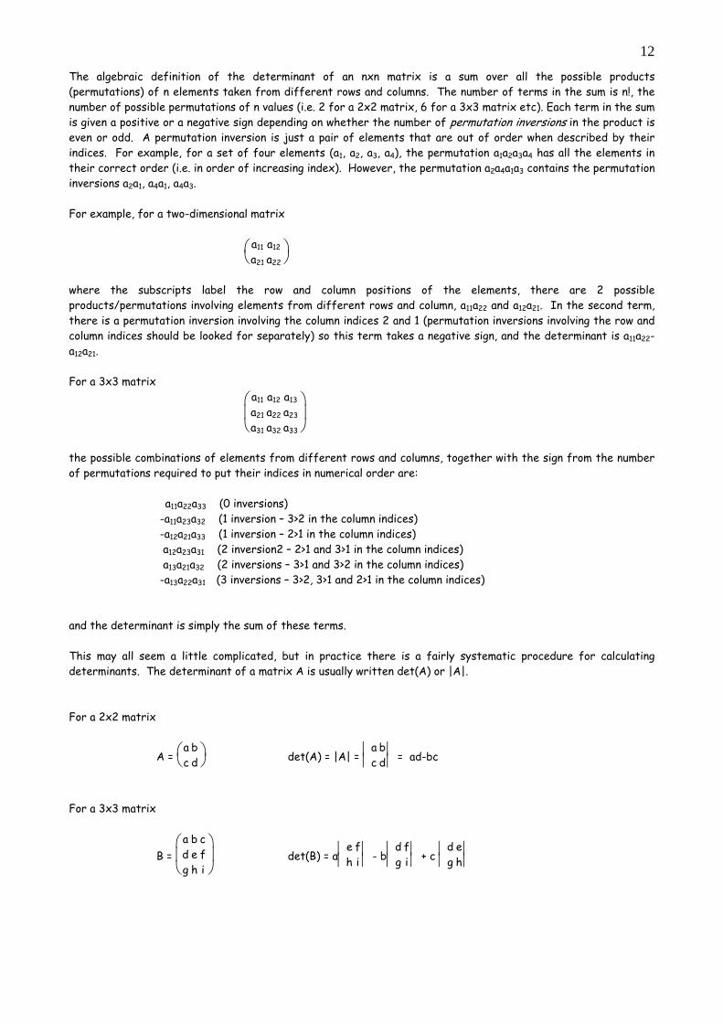
and the determinant is simply the sum of these terms. This may all seem a little complicated, but in practice there is a fairly systematic procedure for calculating determinants. The determinant of a matrix A is usually written det(A) or |A|. For a 2x2 matrix

A = ⎝⎛

⎠⎞a b

c d det(A) = |A| = ⎪⎪

⎪⎪a b

c d = ad-bc

For a 3x3 matrix

B = ⎝⎜⎛

⎠⎟⎞a b c

d e fg h i

det(B) = a⎪⎪

⎪⎪e f

h i - b⎪⎪

⎪⎪d f

g i + c ⎪⎪

⎪⎪d e

g h

13

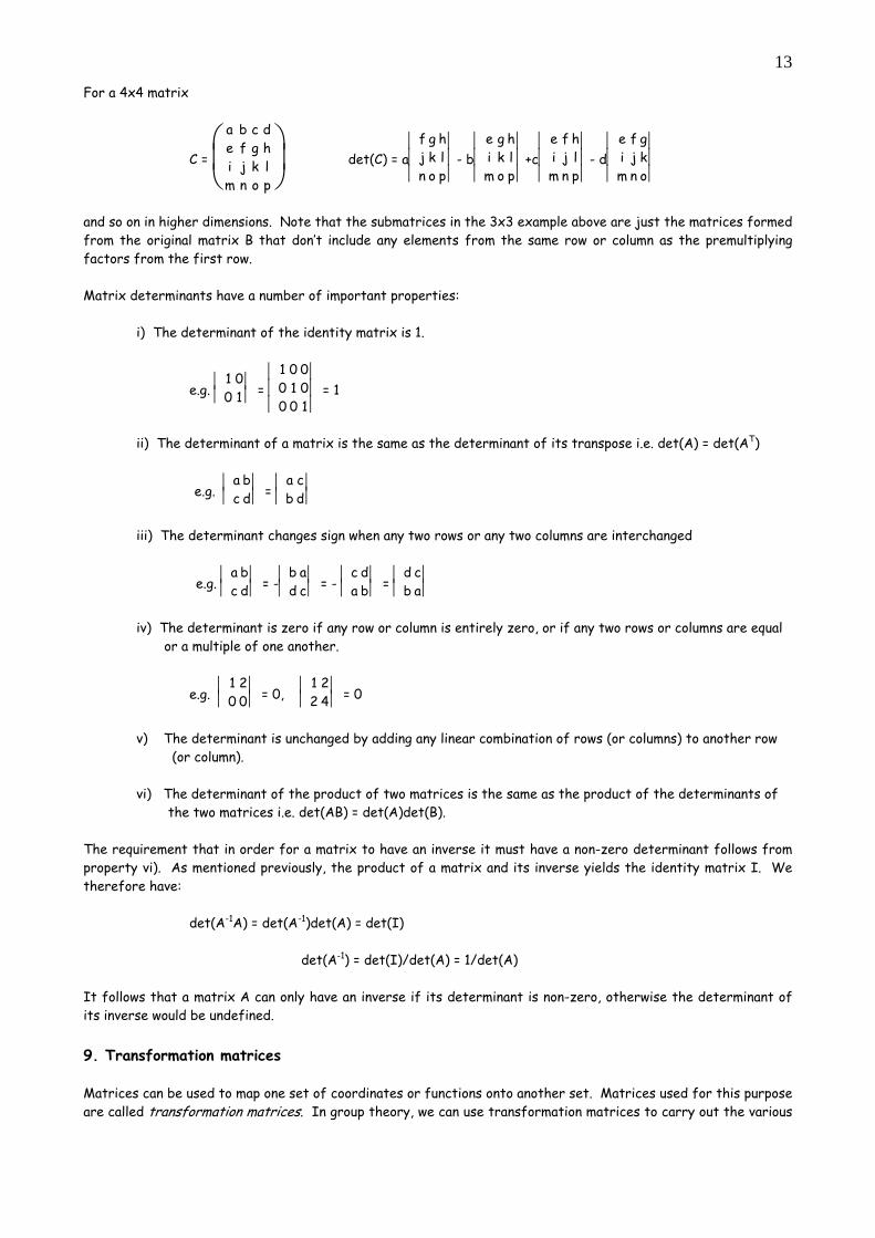
For a 4x4 matrix

C =

⎝⎜⎛

⎠⎟⎞a b c d

e f g hi j k lm n o p

det(C) = a⎪⎪⎪

⎪⎪⎪f g h

j k ln o p

- b⎪⎪⎪

⎪⎪⎪e g h

i k lm o p

+c⎪⎪⎪

⎪⎪⎪e f h

i j lm n p

- d⎪⎪⎪

⎪⎪⎪e f g

i j km n o

and so on in higher dimensions. Note that the submatrices in the 3x3 example above are just the matrices formed from the original matrix B that don’t include any elements from the same row or column as the premultiplying factors from the first row. Matrix determinants have a number of important properties: i) The determinant of the identity matrix is 1.

e.g. ⎪⎪

⎪⎪1 0

0 1 = ⎪⎪⎪

⎪⎪⎪1 0 0

0 1 00 0 1

= 1

ii) The determinant of a matrix is the same as the determinant of its transpose i.e. det(A) = det(AT)

e.g. ⎪⎪

⎪⎪a b

c d = ⎪⎪

⎪⎪a c

b d

iii) The determinant changes sign when any two rows or any two columns are interchanged

e.g. ⎪⎪

⎪⎪a b

c d = -⎪⎪

⎪⎪b a

d c = - ⎪⎪

⎪⎪c d

a b = ⎪⎪

⎪⎪d c

b a

iv) The determinant is zero if any row or column is entirely zero, or if any two rows or columns are equal or a multiple of one another.

e.g. ⎪⎪

⎪⎪1 2

0 0 = 0, ⎪⎪

⎪⎪1 2

2 4 = 0

v) The determinant is unchanged by adding any linear combination of rows (or columns) to another row (or column). vi) The determinant of the product of two matrices is the same as the product of the determinants of the two matrices i.e. det(AB) = det(A)det(B).

The requirement that in order for a matrix to have an inverse it must have a non-zero determinant follows from property vi). As mentioned previously, the product of a matrix and its inverse yields the identity matrix I. We therefore have: det(A-1A) = det(A-1)det(A) = det(I) det(A-1) = det(I)/det(A) = 1/det(A) It follows that a matrix A can only have an inverse if its determinant is non-zero, otherwise the determinant of its inverse would be undefined. 9. Transformation matrices Matrices can be used to map one set of coordinates or functions onto another set. Matrices used for this purpose are called transformation matrices. In group theory, we can use transformation matrices to carry out the various

14

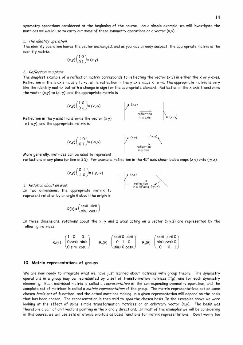
symmetry operations considered at the beginning of the course. As a simple example, we will investigate the matrices we would use to carry out some of these symmetry operations on a vector (x,y). 1. The identity operation The identity operation leaves the vector unchanged, and as you may already suspect, the appropriate matrix is the identity matrix.

(x,y) ⎝⎛

⎠⎞1 0

0 1 = (x,y)

2. Reflection in a plane The simplest example of a reflection matrix corresponds to reflecting the vector (x,y) in either the x or y axes. Reflection in the x axis maps y to –y, while reflection in the y axis maps x to -x. The appropriate matrix is very like the identity matrix but with a change in sign for the appropriate element. Reflection in the x axis transforms the vector (x,y) to (x,-y), and the appropriate matrix is

(x,y) ⎝⎛

⎠⎞1 0

0 -1 = (x,-y) Reflection in the y axis transforms the vector (x,y) to (-x,y), and the appropriate matrix is

(x,y) ⎝⎛

⎠⎞-1 0

0 1 = (-x,y) More generally, matrices can be used to represent reflections in any plane (or line in 2D). For example, reflection in the 45° axis shown below maps (x,y) onto (-y,x).

(x,y) ⎝⎛

⎠⎞0 -1

-1 0 = (-y,-x) 3. Rotation about an axis. In two dimensions, the appropriate matrix to represent rotation by an angle θ about the origin is

R(θ) = ⎝⎛

⎠⎞cosθ -sinθ

sinθ cosθ

In three dimensions, rotations about the x, y and z axes acting on a vector (x,y,z) are represented by the following matrices.

Rx(θ) = ⎝⎜⎛

⎠⎟⎞1 0 0

0 cosθ -sinθ0 sinθ cosθ

Ry(θ) = ⎝⎜⎛

⎠⎟⎞cosθ 0 -sinθ

0 1 0sinθ 0 cosθ

Rz(θ) = ⎝⎜⎛

⎠⎟⎞cosθ -sinθ 0

sinθ cosθ 00 0 1

10. Matrix representations of groups We are now ready to integrate what we have just learned about matrices with group theory. The symmetry operations in a group may be represented by a set of transformation matrices Γ(g), one for each symmetry element g. Each individual matrix is called a representative of the corresponding symmetry operation, and the complete set of matrices is called a matrix representation of the group. The matrix representatives act on some chosen basis set of functions, and the actual matrices making up a given representation will depend on the basis that has been chosen. The representation is then said to span the chosen basis. In the examples above we were looking at the effect of some simple transformation matrices on an arbitrary vector (x,y). The basis was therefore a pair of unit vectors pointing in the x and y directions. In most of the examples we will be considering in this course, we will use sets of atomic orbitals as basis functions for matrix representations. Don’t worry too

(x,y)

(x,-y)reflectionin x axis

(x,y) (-x,y)

reflectionin y axis

(x,y)

(-y,-x)reflection

in a 45°axis

15

much if these ideas seem a little abstract at the moment – they should become clearer in the next section when we look at some examples. Before proceeding any further, we must check that a matrix representation of a group obeys all of the rules set out in the formal mathematical definition of a group. 1. The first rule is that the group must include the identity operation E (the ‘do nothing’ operation). We

showed above that the matrix representative of the identity operation is simply the identity matrix. As a consequence, every matrix representation includes the appropriate identity matrix.

2. The second rule is that the combination of any pair of elements must also be an element of the group (the

group property). If we multiply together any two matrix representatives, we should get a new matrix which is a representative of another symmetry operation of the group. In fact, matrix representatives multiply together to give new representatives in exactly the same way as symmetry operations combine according to the group multiplication table. For example, in the C3v point group, we showed that the combined symmetry operation C3σv is equivalent to σv’’. In a matrix representation of the group, if the matrix representatives of C3 and σv are multiplied together, the result will be the representative of σv’’.

3. The third rule states that every operation must have an inverse, which is also a member of the group.

The combined effect of carrying out an operation and its inverse is the same as the identity operation. It is fairly easy to show that matrix representatives satisfy this criterion. For example, the inverse of a reflection is another reflection, identical to the first. In matrix terms we would therefore expect that a reflection matrix was its own inverse, and that two identical reflection matrices multiplied together would give the identity matrix. This turns out to be true, and can be verified using any of the reflection matrices in the examples above. The inverse of a rotation matrix is another rotation matrix corresponding to a rotation of the opposite sense to the first.

4. The final rule states that the rule of combination of symmetry elements in a group must be associative.

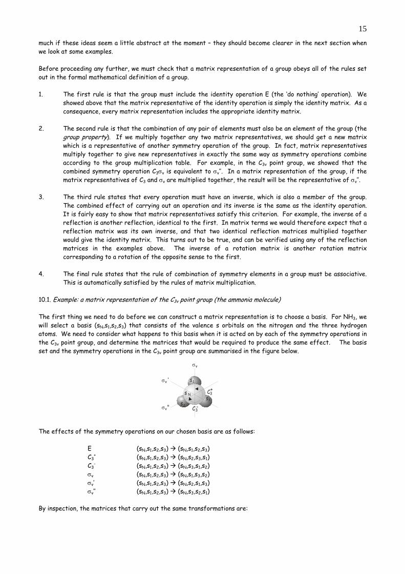
This is automatically satisfied by the rules of matrix multiplication. 10.1. Example: a matrix representation of the C3v point group (the ammonia molecule) The first thing we need to do before we can construct a matrix representation is to choose a basis. For NH3, we will select a basis (sN,s1,s2,s3) that consists of the valence s orbitals on the nitrogen and the three hydrogen atoms. We need to consider what happens to this basis when it is acted on by each of the symmetry operations in the C3v point group, and determine the matrices that would be required to produce the same effect. The basis set and the symmetry operations in the C3v point group are summarised in the figure below.

σv

σv'

σv"

C+3

C -3

s1

s2

s3

s N

The effects of the symmetry operations on our chosen basis are as follows:

E (sN,s1,s2,s3) (sN,s1,s2,s3) C3

+ (sN,s1,s2,s3) (sN,s2,s3,s1) C3

- (sN,s1,s2,s3) (sN,s3,s1,s2) σv (sN,s1,s2,s3) (sN,s1,s3,s2) σv’ (sN,s1,s2,s3) (sN,s2,s1,s3) σv’’ (sN,s1,s2,s3) (sN,s3,s2,s1)

By inspection, the matrices that carry out the same transformations are:

16

Γ(E) (sN,s1,s2,s3)

⎝⎜⎛

⎠⎟⎞ 1 0 0 0

0 1 0 0 0 0 1 0 0 0 0 1

= (sN,s1,s2,s3)

Γ(C3+) (sN,s1,s2,s3)

⎝⎜⎛

⎠⎟⎞ 1 0 0 0

0 0 0 1 0 1 0 0 0 0 1 0

= (sN,s2,s3,s1)

Γ(C3-) (sN,s1,s2,s3)

⎝⎜⎛

⎠⎟⎞ 1 0 0 0

0 0 1 0 0 0 0 1 0 1 0 0

= (sN,s3,s1,s2)

Γ (σv) (sN,s1,s2,s3)

⎝⎜⎛

⎠⎟⎞ 1 0 0 0

0 1 0 0 0 0 0 1 0 0 1 0

= (sN,s1,s3,s2)

Γ (σv’) (sN,s1,s2,s3)

⎝⎜⎛

⎠⎟⎞ 1 0 0 0

0 0 1 0 0 1 0 0 0 0 0 1

= (sN,s2,s1,s3)

Γ (σv’’) (sN,s1,s2,s3)

⎝⎜⎛

⎠⎟⎞ 1 0 0 0

0 0 0 1 0 0 1 0 0 1 0 0

= (sN,s3,s2,s1)

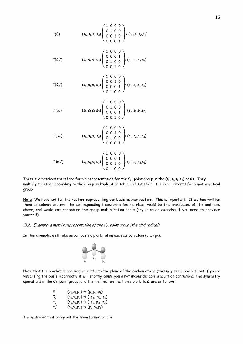
These six matrices therefore form a representation for the C3v point group in the (sN,s1,s2,s3) basis. They multiply together according to the group multiplication table and satisfy all the requirements for a mathematical group. Note: We have written the vectors representing our basis as row vectors. This is important. If we had written them as column vectors, the corresponding transformation matrices would be the transposes of the matrices above, and would not reproduce the group multiplication table (try it as an exercise if you need to convince yourself). 10.2. Example: a matrix representation of the C2v point group (the allyl radical) In this example, we’ll take as our basis a p orbital on each carbon atom (p1,p2,p3).

p1

p2p3

Note that the p orbitals are perpendicular to the plane of the carbon atoms (this may seem obvious, but if you’re visualising the basis incorrectly it will shortly cause you a not inconsiderable amount of confusion). The symmetry operations in the C2v point group, and their effect on the three p orbitals, are as follows:

E (p1,p2,p3) (p1,p2,p3) C2 (p1,p2,p3) (-p3,-p2,-p1) σv (p1,p2,p3) (-p1,-p2,-p3) σv’ (p1,p2,p3) (p3,p2,p1)

The matrices that carry out the transformation are

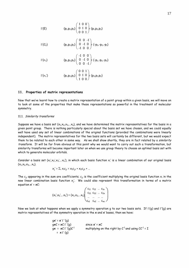
17

Γ(E) (p1,p2,p3) ⎝⎜⎛

⎠⎟⎞ 1 0 0

0 1 0 0 0 1

= (p1,p2,p3)

Γ(C2) (p1,p2,p3) ⎝⎜⎛

⎠⎟⎞ 0 0 -1

0 -1 0 -1 0 0

= (-p3,-p2,-p1)

Γ(σv) (p1,p2,p3) ⎝⎜⎛

⎠⎟⎞ -1 0 0

0 -1 0 0 0 -1

= (-p1,-p2,-p3)

Γ(σv’) (p1,p2,p3) ⎝⎜⎛

⎠⎟⎞ 0 0 1

0 1 0 1 0 0

= (p3,p1,p2)

11. Properties of matrix representations Now that we’ve learnt how to create a matrix representation of a point group within a given basis, we will move on to look at some of the properties that make these representations so powerful in the treatment of molecular symmetry. 11.1. Similarity transforms Suppose we have a basis set (x1,x2,x3,…xn), and we have determined the matrix representatives for the basis in a given point group. There is nothing particularly special about the basis set we have chosen, and we could equally well have used any set of linear combinations of the original functions (provided the combinations were linearly independent). The matrix representatives for the two basis sets will certainly be different, but we would expect them to be related to each other in some way. As we shall show shortly, they are in fact related by a similarity transform. It will be far from obvious at this point why we would want to carry out such a transformation, but similarity transforms will become important later on when we use group theory to choose an optimal basis set with which to generate molecular orbitals. Consider a basis set (x1’,x2’,x3’,…xn’), in which each basis function xi’ is a linear combination of our original basis (x1,x2,x3,…xn). xj’ = Σi xicji = x1cj1 + x2cj2 + … The cji appearing in the sum are coefficients; cji is the coefficient multiplying the original basis function xi in the new linear combination basis function xj’. We could also represent this transformation in terms of a matrix equation x’ = xC:

(x1’,x2’,…xn’) = (x1,x2,…xn)

⎝⎜⎛

⎠⎟⎞ c11 c12 … c1n

c21 c22 … c2n

… … … …cn1 cn2 … cnn

Now we look at what happens when we apply a symmetry operation g to our two basis sets. If Γ(g) and Γ’(g) are matrix representatives of the symmetry operation in the x and x’ bases, then we have: gx’ = x’ Γ ’(g) gxC = xC Γ ’(g) since x’ = xC gx = xC Γ ’(g)C-1 multiplying on the right by C-1 and using CC-1 = I = x Γ (g)

18

We can therefore identify the similarity transform relating Γ(g), the matrix representative in our original basis, to Γ ’(g), the representative in the transformed basis. The transform depends only on the matrix of coefficients used to transform the basis functions.

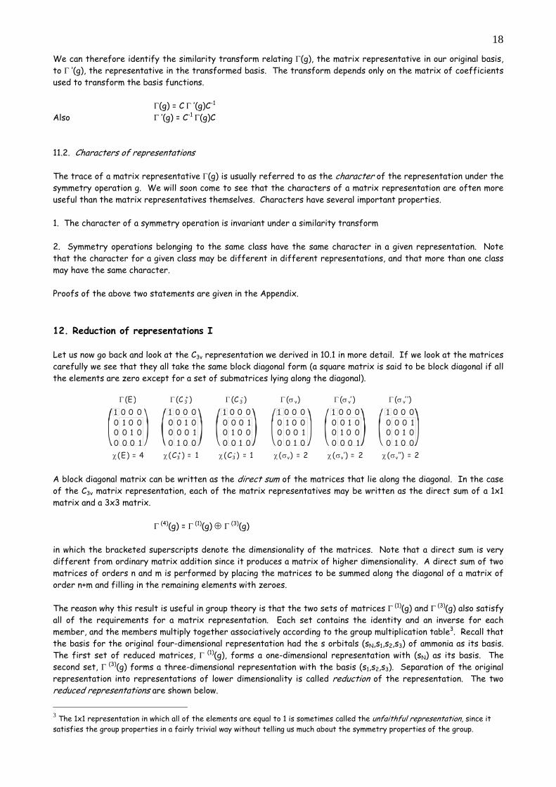
Γ(g) = C Γ ’(g)C-1 Also Γ ’(g) = C-1 Γ(g)C 11.2. Characters of representations The trace of a matrix representative Γ(g) is usually referred to as the character of the representation under the symmetry operation g. We will soon come to see that the characters of a matrix representation are often more useful than the matrix representatives themselves. Characters have several important properties. 1. The character of a symmetry operation is invariant under a similarity transform 2. Symmetry operations belonging to the same class have the same character in a given representation. Note that the character for a given class may be different in different representations, and that more than one class may have the same character. Proofs of the above two statements are given in the Appendix. 12. Reduction of representations I Let us now go back and look at the C3v representation we derived in 10.1 in more detail. If we look at the matrices carefully we see that they all take the same block diagonal form (a square matrix is said to be block diagonal if all the elements are zero except for a set of submatrices lying along the diagonal).

Γ (E)

χ(E) = 4

Γ (C )3+

χ(C ) = 13+

Γ (C )3-

χ(C ) = 13-

Γ σ( v)

χ ) = 2(σv

Γ σ( ’)v

χ( ’) = 2σv

Γ σ( ’ ’)v

χ( ’’) = 2σv

1 0 0 00 1 0 00 0 1 00 0 0 1

1 0 0 00 0 0 10 1 0 00 0 1 0

1 0 0 00 0 1 00 0 0 10 1 0 0

1 0 0 00 1 0 00 0 0 10 0 1 0

1 0 0 00 0 1 0 0 1 0 00 0 0 1

1 0 0 00 0 0 10 0 1 00 1 0 0

A block diagonal matrix can be written as the direct sum of the matrices that lie along the diagonal. In the case of the C3v matrix representation, each of the matrix representatives may be written as the direct sum of a 1x1 matrix and a 3x3 matrix.

Γ (4)(g) = Γ (1)(g) ⊕ Γ (3)(g) in which the bracketed superscripts denote the dimensionality of the matrices. Note that a direct sum is very different from ordinary matrix addition since it produces a matrix of higher dimensionality. A direct sum of two matrices of orders n and m is performed by placing the matrices to be summed along the diagonal of a matrix of order n+m and filling in the remaining elements with zeroes. The reason why this result is useful in group theory is that the two sets of matrices Γ (1)(g) and Γ (3)(g) also satisfy all of the requirements for a matrix representation. Each set contains the identity and an inverse for each member, and the members multiply together associatively according to the group multiplication table3. Recall that the basis for the original four-dimensional representation had the s orbitals (sN,s1,s2,s3) of ammonia as its basis. The first set of reduced matrices, Γ (1)(g), forms a one-dimensional representation with (sN) as its basis. The second set, Γ (3)(g) forms a three-dimensional representation with the basis (s1,s2,s3). Separation of the original representation into representations of lower dimensionality is called reduction of the representation. The two reduced representations are shown below.

3 The 1x1 representation in which all of the elements are equal to 1 is sometimes called the unfaithful representation, since it satisfies the group properties in a fairly trivial way without telling us much about the symmetry properties of the group.

19

g E C3

+ C3- σv σv’ σv’’

1D representation spanned Γ (1)(g) (1) (1) (1) (1) (1) (1) by (sN)

Γ (3)(g) ⎝⎜⎛

⎠⎟⎞ 1 0 0

0 1 0 0 0 1

⎝⎜⎛

⎠⎟⎞ 0 1 0

0 0 1 1 0 0

⎝⎜⎛

⎠⎟⎞ 0 0 1

1 0 0 0 1 0

⎝⎜⎛

⎠⎟⎞ 1 0 0

0 0 1 0 1 0

⎝⎜⎛

⎠⎟⎞ 0 1 0

1 0 0 0 0 1

⎝⎜⎛

⎠⎟⎞ 0 0 1

0 1 0 1 0 0

3D representation spanned by (s1,s2,s3)

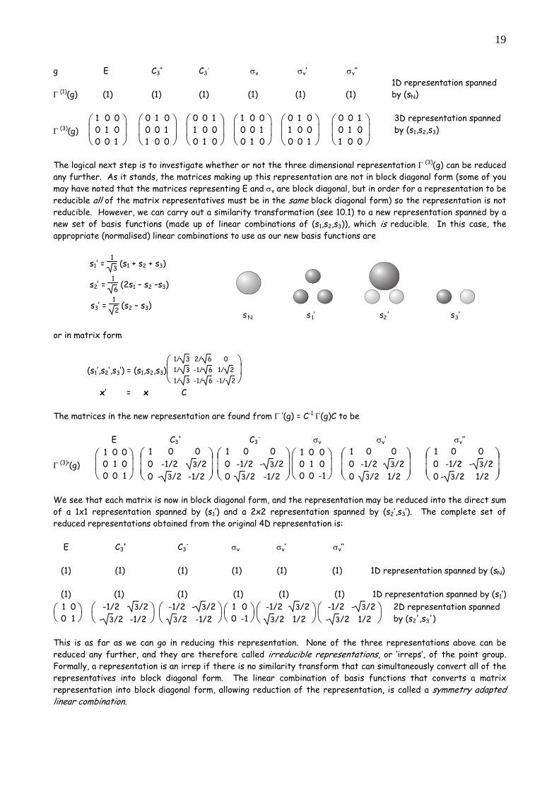
The logical next step is to investigate whether or not the three dimensional representation Γ (3)(g) can be reduced any further. As it stands, the matrices making up this representation are not in block diagonal form (some of you may have noted that the matrices representing E and σv are block diagonal, but in order for a representation to be reducible all of the matrix representatives must be in the same block diagonal form) so the representation is not reducible. However, we can carry out a similarity transformation (see 10.1) to a new representation spanned by a new set of basis functions (made up of linear combinations of (s1,s2,s3)), which is reducible. In this case, the appropriate (normalised) linear combinations to use as our new basis functions are

s1’ = 13 (s1 + s2 + s3)

s2’ = 16 (2s1 – s2 –s3)

s3’ = 12 (s2 – s3)

or in matrix form

(s1’,s2’,s3’) = (s1,s2,s3)⎝⎜⎛

⎠⎟⎞ 1/ 3 2/ 6 0

1/ 3 -1/ 6 1/ 2 1/ 3 -1/ 6 -1/ 2

x’ = x C The matrices in the new representation are found from Γ ’(g) = C-1 Γ(g)C to be E C3

+ C3- σv σv’ σv’’

Γ (3)’(g) ⎝⎜⎛

⎠⎟⎞ 1 0 0

0 1 0 0 0 1

⎝⎜⎜⎛

⎠⎟⎟⎞

1 0 0 0 -1/2 3/2 0 - 3/2 -1/2

⎝⎜⎜⎛

⎠⎟⎟⎞

1 0 0 0 -1/2 - 3/2 0 3/2 -1/2

⎝⎜⎛

⎠⎟⎞ 1 0 0

0 1 0 0 0 -1

⎝⎜⎜⎛

⎠⎟⎟⎞

1 0 0 0 -1/2 3/2 0 3/2 1/2

⎝⎜⎜⎛

⎠⎟⎟⎞

1 0 0 0 -1/2 - 3/2 0 - 3/2 1/2

We see that each matrix is now in block diagonal form, and the representation may be reduced into the direct sum of a 1x1 representation spanned by (s1’) and a 2x2 representation spanned by (s2’,s3’). The complete set of reduced representations obtained from the original 4D representation is: E C3

+ C3- σv σv’ σv’’

(1) (1) (1) (1) (1) (1) 1D representation spanned by (sN) (1) (1) (1) (1) (1) (1) 1D representation spanned by (s1’)

⎝⎛

⎠⎞ 1 0

0 1 ⎝⎛

⎠⎞ -1/2 3/2

- 3/2 -1/2 ⎝⎛

⎠⎞ -1/2 - 3/2

3/2 -1/2 ⎝⎛

⎠⎞ 1 0

0 -1 ⎝⎛

⎠⎞ -1/2 3/2

3/2 1/2 ⎝⎛

⎠⎞-1/2 - 3/2

- 3/2 1/2 2D representation spanned by (s2',s3')

This is as far as we can go in reducing this representation. None of the three representations above can be reduced any further, and they are therefore called irreducible representations, or ‘irreps’, of the point group. Formally, a representation is an irrep if there is no similarity transform that can simultaneously convert all of the representatives into block diagonal form. The linear combination of basis functions that converts a matrix representation into block diagonal form, allowing reduction of the representation, is called a symmetry adapted linear combination.

sN s ’1 s ’2 s ’3

20

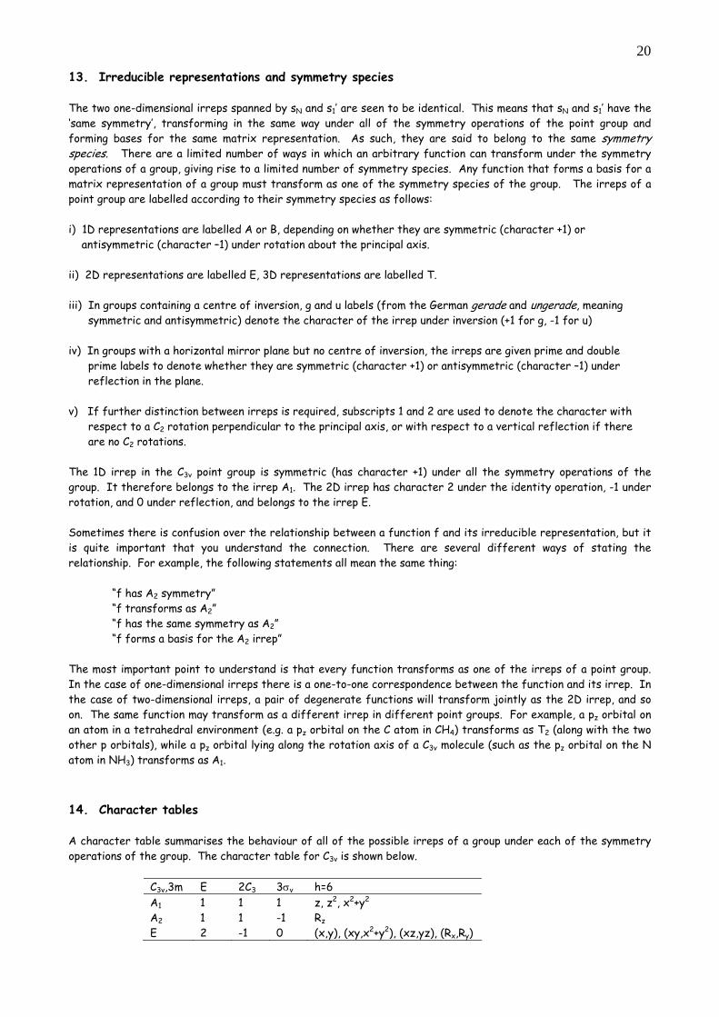
13. Irreducible representations and symmetry species The two one-dimensional irreps spanned by sN and s1’ are seen to be identical. This means that sN and s1’ have the ‘same symmetry’, transforming in the same way under all of the symmetry operations of the point group and forming bases for the same matrix representation. As such, they are said to belong to the same symmetry species. There are a limited number of ways in which an arbitrary function can transform under the symmetry operations of a group, giving rise to a limited number of symmetry species. Any function that forms a basis for a matrix representation of a group must transform as one of the symmetry species of the group. The irreps of a point group are labelled according to their symmetry species as follows: i) 1D representations are labelled A or B, depending on whether they are symmetric (character +1) or antisymmetric (character –1) under rotation about the principal axis. ii) 2D representations are labelled E, 3D representations are labelled T. iii) In groups containing a centre of inversion, g and u labels (from the German gerade and ungerade, meaning symmetric and antisymmetric) denote the character of the irrep under inversion (+1 for g, -1 for u) iv) In groups with a horizontal mirror plane but no centre of inversion, the irreps are given prime and double prime labels to denote whether they are symmetric (character +1) or antisymmetric (character –1) under reflection in the plane. v) If further distinction between irreps is required, subscripts 1 and 2 are used to denote the character with respect to a C2 rotation perpendicular to the principal axis, or with respect to a vertical reflection if there are no C2 rotations. The 1D irrep in the C3v point group is symmetric (has character +1) under all the symmetry operations of the group. It therefore belongs to the irrep A1. The 2D irrep has character 2 under the identity operation, -1 under rotation, and 0 under reflection, and belongs to the irrep E. Sometimes there is confusion over the relationship between a function f and its irreducible representation, but it is quite important that you understand the connection. There are several different ways of stating the relationship. For example, the following statements all mean the same thing: “f has A2 symmetry” “f transforms as A2” “f has the same symmetry as A2” “f forms a basis for the A2 irrep” The most important point to understand is that every function transforms as one of the irreps of a point group. In the case of one-dimensional irreps there is a one-to-one correspondence between the function and its irrep. In the case of two-dimensional irreps, a pair of degenerate functions will transform jointly as the 2D irrep, and so on. The same function may transform as a different irrep in different point groups. For example, a pz orbital on an atom in a tetrahedral environment (e.g. a pz orbital on the C atom in CH4) transforms as T2 (along with the two other p orbitals), while a pz orbital lying along the rotation axis of a C3v molecule (such as the pz orbital on the N atom in NH3) transforms as A1. 14. Character tables A character table summarises the behaviour of all of the possible irreps of a group under each of the symmetry operations of the group. The character table for C3v is shown below.

C3v,3m E 2C3 3σv h=6 A1 1 1 1 z, z2, x2+y2 A2 1 1 -1 Rz E 2 -1 0 (x,y), (xy,x2+y2), (xz,yz), (Rx,Ry)

21

The various sections of the table are as follows:

i) The first element in the table gives the name of the point group, usually in both Schoenflies (C3v) and Hermann-Mauguin (3m) notation. ii) Along the first row are the symmetry operations of the group, E, 2C3 and 3σv, followed by the order h of the group. Because operations in the same class have the same character, symmetry operations are grouped into classes in the character table and not listed separately. iii) In the first column are the irreps of the group. In C3v the irreps are A1, A2 and E (the representation we considered above spans 2A1 + E). iv) The characters of the irreps under each symmetry operation are given in the bulk of the table. v) The final column of the table lists a number of functions that transform as the various irreps of the group. These are the Cartesian axes (x,y,z) the Cartesian products (z2, x2+y2, xy, xz, yz) and the rotations (Rx,Ry,Rz).

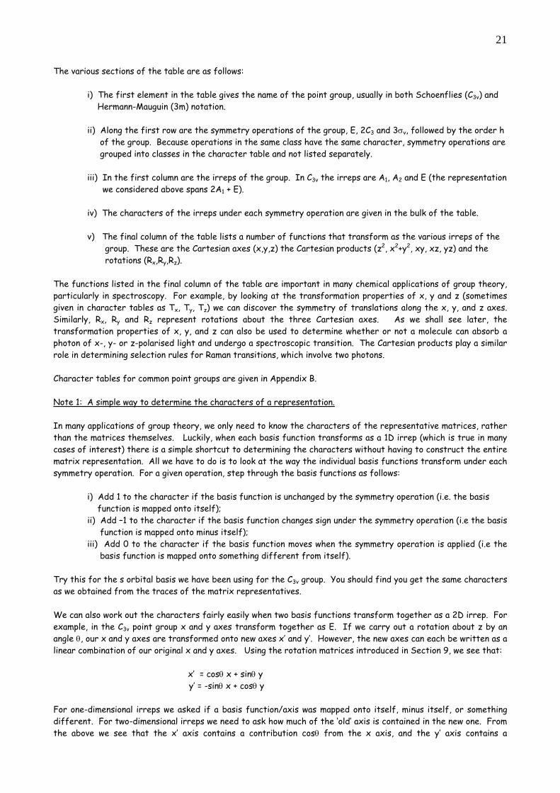
The functions listed in the final column of the table are important in many chemical applications of group theory, particularly in spectroscopy. For example, by looking at the transformation properties of x, y and z (sometimes given in character tables as Tx, Ty, Tz) we can discover the symmetry of translations along the x, y, and z axes. Similarly, Rx, Ry and Rz represent rotations about the three Cartesian axes. As we shall see later, the transformation properties of x, y, and z can also be used to determine whether or not a molecule can absorb a photon of x-, y- or z-polarised light and undergo a spectroscopic transition. The Cartesian products play a similar role in determining selection rules for Raman transitions, which involve two photons. Character tables for common point groups are given in Appendix B. Note 1: A simple way to determine the characters of a representation. In many applications of group theory, we only need to know the characters of the representative matrices, rather than the matrices themselves. Luckily, when each basis function transforms as a 1D irrep (which is true in many cases of interest) there is a simple shortcut to determining the characters without having to construct the entire matrix representation. All we have to do is to look at the way the individual basis functions transform under each symmetry operation. For a given operation, step through the basis functions as follows: i) Add 1 to the character if the basis function is unchanged by the symmetry operation (i.e. the basis function is mapped onto itself); ii) Add –1 to the character if the basis function changes sign under the symmetry operation (i.e the basis function is mapped onto minus itself); iii) Add 0 to the character if the basis function moves when the symmetry operation is applied (i.e the basis function is mapped onto something different from itself). Try this for the s orbital basis we have been using for the C3v group. You should find you get the same characters as we obtained from the traces of the matrix representatives. We can also work out the characters fairly easily when two basis functions transform together as a 2D irrep. For example, in the C3v point group x and y axes transform together as E. If we carry out a rotation about z by an angle θ, our x and y axes are transformed onto new axes x’ and y’. However, the new axes can each be written as a linear combination of our original x and y axes. Using the rotation matrices introduced in Section 9, we see that: x’ = cosθ x + sinθ y y’ = -sinθ x + cosθ y For one-dimensional irreps we asked if a basis function/axis was mapped onto itself, minus itself, or something different. For two-dimensional irreps we need to ask how much of the ‘old’ axis is contained in the new one. From the above we see that the x’ axis contains a contribution cosθ from the x axis, and the y’ axis contains a

22

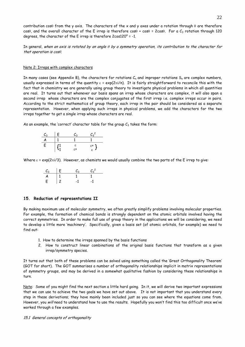
contribution cosθ from the y axis. The characters of the x and y axes under a rotation through θ are therefore cosθ, and the overall character of the E irrep is therefore cosθ + cosθ = 2cosθ. For a C3 rotation through 120 degrees, the character of the E irrep is therefore 2cos120° = -1. In general, when an axis is rotated by an angle θ by a symmetry operation, its contribution to the character for that operation is cosθ. Note 2: Irreps with complex characters In many cases (see Appendix B), the characters for rotations Cn and improper rotations Sn are complex numbers, usually expressed in terms of the quantity ε = exp(2πi/n). It is fairly straightforward to reconcile this with the fact that in chemistry we are generally using group theory to investigate physical problems in which all quantities are real. It turns out that whenever our basis spans an irrep whose characters are complex, it will also span a second irrep whose characters are the complex conjugates of the first irrep i.e. complex irreps occur in pairs. According to the strict mathematics of group theory, each irrep in the pair should be considered as a separate representation. However, when applying such irreps in physical problems, we add the characters for the two irreps together to get a single irrep whose characters are real. As an example, the ‘correct’ character table for the group C3 takes the form:

C3 E C3 C32

A 1 1 1 E {1

1 ε∗ε

εε∗ }

Where ε = exp(2πi/3). However, as chemists we would usually combine the two parts of the E irrep to give:

C3 E C3 C32

A 1 1 1 E 2 -1 -1

15. Reduction of representations II By making maximum use of molecular symmetry, we often greatly simplify problems involving molecular properties. For example, the formation of chemical bonds is strongly dependent on the atomic orbitals involved having the correct symmetries. In order to make full use of group theory in the applications we will be considering, we need to develop a little more ‘machinery’. Specifically, given a basis set (of atomic orbitals, for example) we need to find out: 1. How to determine the irreps spanned by the basis functions

2. How to construct linear combinations of the original basis functions that transform as a given irrep/symmetry species.

It turns out that both of these problems can be solved using something called the ‘Great Orthogonality Theorem’ (GOT for short). The GOT summarises a number of orthogonality relationships implicit in matrix representations of symmetry groups, and may be derived in a somewhat qualitative fashion by considering these relationships in turn. Note: Some of you might find the next section a little hard going. In it, we will derive two important expressions that we can use to achieve the two goals we have set out above. It is not important that you understand every step in these derivations; they have mainly been included just so you can see where the equations come from. However, you will need to understand how to use the results. Hopefully you won’t find this too difficult once we’ve worked through a few examples. 15.1 General concepts of orthogonality

23

You are probably already familiar with the geometric concept of orthogonality. Two vectors are orthogonal if their dot product (i.e. the projection of one vector onto the other) is zero. An example of a pair of orthogonal vectors is provded by the x and y Cartesian unit vectors.

x.y = 0

A consequence of the orthogonality of x and y is that any general vector in the xy plane may be written as a linear combination of these two basis vectors.

r = ax + by

Mathematical functions may also be orthogonal. Two functions, f1(x) and f2(x), are defined to be orthogonal if the

integral over their product is equal to zero i.e. ⌡⌠

f1(x) f2(x) dx = δ12. This simply means that there must be ‘no

overlap’ between orthogonal functions, which is the same as the orthogonality requirement for vectors, above. In the same way as for vectors, any general function may be written as a linear combination of a suitably chosen set of orthogonal basis functions. For example, the Legendre polynomials Pn(x) form an orthogonal basis set for functions of one variable x.

f(x) = Σn cn Pn(x)

15.2 Orthogonality relationships in group theory The irreps of a point group satisfy a number of orthogonality relationships: 1. If corresponding matrix elements in all of the matrix representatives of an irrep are squared and added together, the result is equal to the order of the group divided by the dimensionality of the irrep. i.e.

Σg Γk(g)ij Γk(g)ij = hdk

(15.2.1)

where k labels the irrep, i and j label the row and column position within the irrep, h is the order of the group, and dk is the order of the irrep. e.g. The order of the group C3v is 6. If we apply the above operation to the first element in the 2x2 (E) irrep derived in Section 12, the result should be equal to h/dk = 6/2 = 3. Carrying out this operation gives:

(1)2 + (-½)2 + (-½)2 + (1)2 + (-½)2 + (-½)2 = 1 + ¼ + ¼ + 1 + ¼ + ¼ = 3

2. If instead of summing the squares of matrix elements in an irrep, we sum the product of two different elements from within each matrix, the result is equal to zero. i.e.

Σg Γk(g)ij Γk(g)i'j' = 0 (15.2.2)

where i ≠i’ and/or j ≠j’. e.g. if we perform this operation using the two elements in the first row of the 2D irrep used in 1., we get:

y

x

yr

x

24

(1)(0) + (-½)(3

2 ) + (-½)(-3

2 ) + (1)(0) + (-½)(3

2 ) + (-½)(-3

2 ) = 0 + 3

4 - 3

4 + 0 – 3

4 + 3

4 = 0

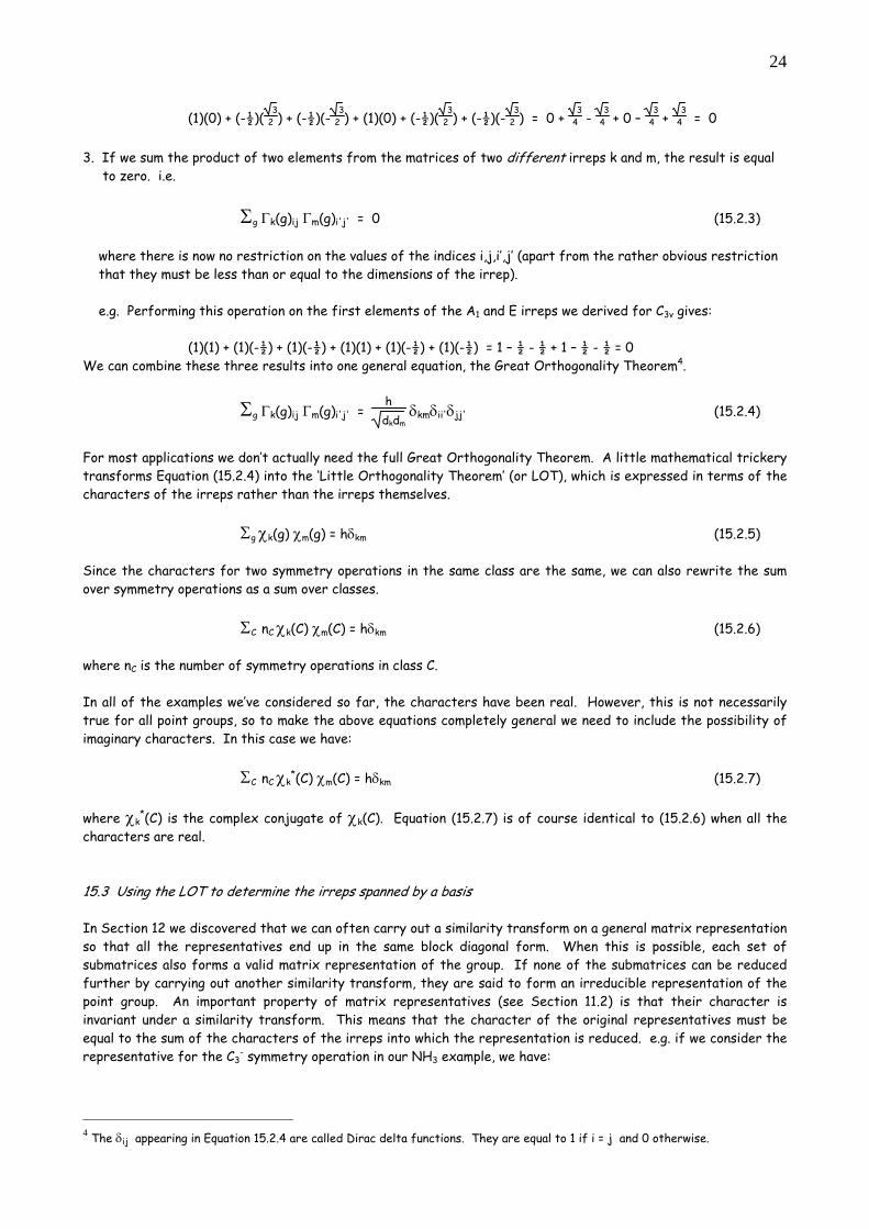
3. If we sum the product of two elements from the matrices of two different irreps k and m, the result is equal to zero. i.e.

Σg Γk(g)ij Γm(g)i'j' = 0 (15.2.3) where there is now no restriction on the values of the indices i,j,i’,j’ (apart from the rather obvious restriction that they must be less than or equal to the dimensions of the irrep). e.g. Performing this operation on the first elements of the A1 and E irreps we derived for C3v gives: (1)(1) + (1)(-½) + (1)(-½) + (1)(1) + (1)(-½) + (1)(-½) = 1 – ½ - ½ + 1 – ½ - ½ = 0 We can combine these three results into one general equation, the Great Orthogonality Theorem4.

Σg Γk(g)ij Γm(g)i'j' = hdkdm

δkmδii'δjj' (15.2.4)

For most applications we don’t actually need the full Great Orthogonality Theorem. A little mathematical trickery transforms Equation (15.2.4) into the ‘Little Orthogonality Theorem’ (or LOT), which is expressed in terms of the characters of the irreps rather than the irreps themselves. Σg χk(g) χm(g) = hδkm (15.2.5) Since the characters for two symmetry operations in the same class are the same, we can also rewrite the sum over symmetry operations as a sum over classes. ΣC nC χk(C) χm(C) = hδkm (15.2.6) where nC is the number of symmetry operations in class C. In all of the examples we’ve considered so far, the characters have been real. However, this is not necessarily true for all point groups, so to make the above equations completely general we need to include the possibility of imaginary characters. In this case we have: ΣC nC χk

*(C) χm(C) = hδkm (15.2.7) where χk

*(C) is the complex conjugate of χk(C). Equation (15.2.7) is of course identical to (15.2.6) when all the characters are real. 15.3 Using the LOT to determine the irreps spanned by a basis In Section 12 we discovered that we can often carry out a similarity transform on a general matrix representation so that all the representatives end up in the same block diagonal form. When this is possible, each set of submatrices also forms a valid matrix representation of the group. If none of the submatrices can be reduced further by carrying out another similarity transform, they are said to form an irreducible representation of the point group. An important property of matrix representatives (see Section 11.2) is that their character is invariant under a similarity transform. This means that the character of the original representatives must be equal to the sum of the characters of the irreps into which the representation is reduced. e.g. if we consider the representative for the C3

- symmetry operation in our NH3 example, we have:

4 The δij appearing in Equation 15.2.4 are called Dirac delta functions. They are equal to 1 if i = j and 0 otherwise.

25

⎝⎜⎛

⎠⎟⎞ 1 0 0 0

0 0 0 1 0 1 0 0 0 0 1 0

similarity transform

⎝⎜⎛

⎠⎟⎞ 1 0 0 0

0 1 0 0 0 0 -1/2 - 3/2 0 0 3/2 -1/2

= ( 1 ) ⊕ ( 1 ) ⊕ ⎝⎛

⎠⎞ -1/2 - 3/2

3/2 -1/2

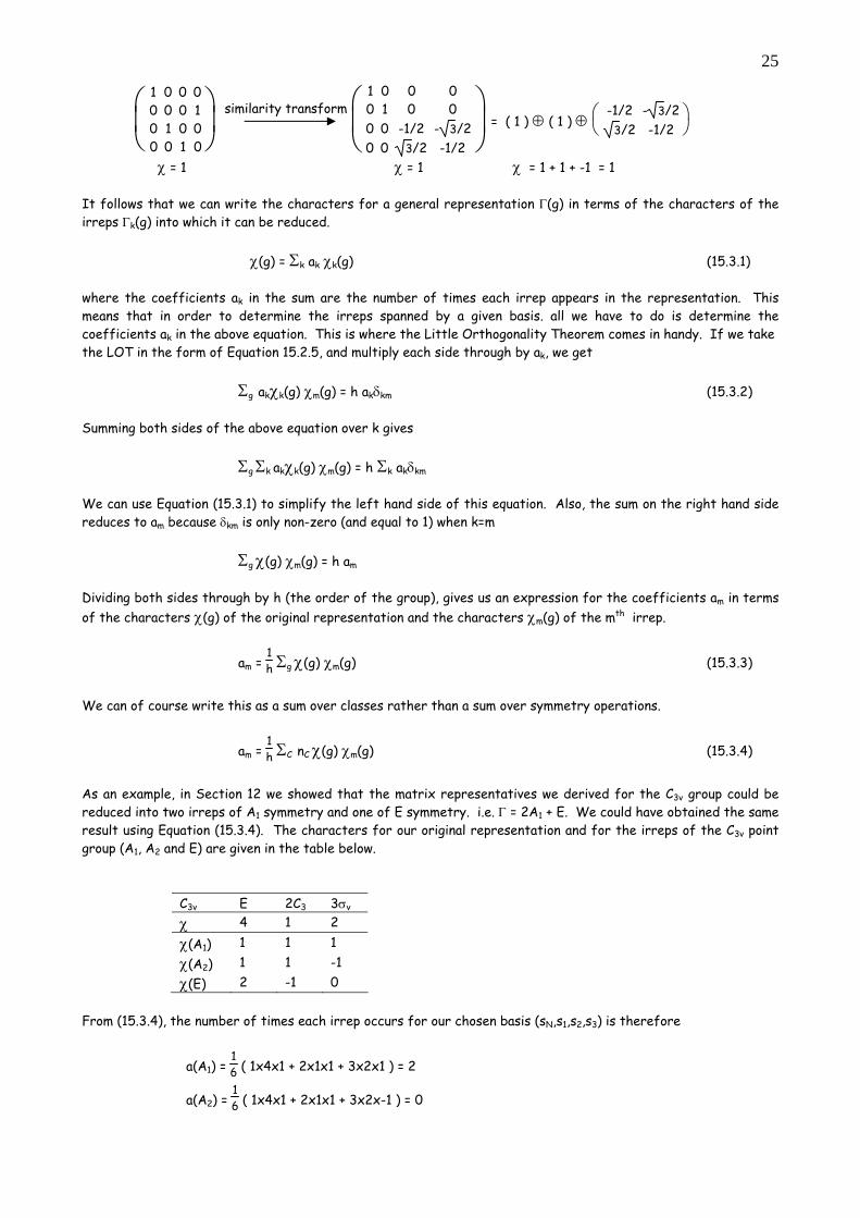
χ = 1 χ = 1 χ = 1 + 1 + -1 = 1 It follows that we can write the characters for a general representation Γ(g) in terms of the characters of the irreps Γk(g) into which it can be reduced.

χ(g) = Σk ak χk(g) (15.3.1)

where the coefficients ak in the sum are the number of times each irrep appears in the representation. This means that in order to determine the irreps spanned by a given basis. all we have to do is determine the coefficients ak in the above equation. This is where the Little Orthogonality Theorem comes in handy. If we take the LOT in the form of Equation 15.2.5, and multiply each side through by ak, we get

Σg akχk(g) χm(g) = h akδkm (15.3.2)

Summing both sides of the above equation over k gives Σg Σk akχk(g) χm(g) = h Σk akδkm We can use Equation (15.3.1) to simplify the left hand side of this equation. Also, the sum on the right hand side reduces to am because δkm is only non-zero (and equal to 1) when k=m Σg χ(g) χm(g) = h am Dividing both sides through by h (the order of the group), gives us an expression for the coefficients am in terms of the characters χ(g) of the original representation and the characters χm(g) of the mth irrep.

am = 1h Σg χ(g) χm(g) (15.3.3)

We can of course write this as a sum over classes rather than a sum over symmetry operations.

am = 1h ΣC nC χ(g) χm(g) (15.3.4)

As an example, in Section 12 we showed that the matrix representatives we derived for the C3v group could be reduced into two irreps of A1 symmetry and one of E symmetry. i.e. Γ = 2A1 + E. We could have obtained the same result using Equation (15.3.4). The characters for our original representation and for the irreps of the C3v point group (A1, A2 and E) are given in the table below.

C3v E 2C3 3σv χ 4 1 2 χ(A1) 1 1 1 χ(A2) 1 1 -1 χ(E) 2 -1 0

From (15.3.4), the number of times each irrep occurs for our chosen basis (sN,s1,s2,s3) is therefore

a(A1) = 16 ( 1x4x1 + 2x1x1 + 3x2x1 ) = 2

a(A2) = 16 ( 1x4x1 + 2x1x1 + 3x2x-1 ) = 0

26

a(E) = 16 ( 1x4x2 + 2x1x-1 + 3x2x0 ) = 1

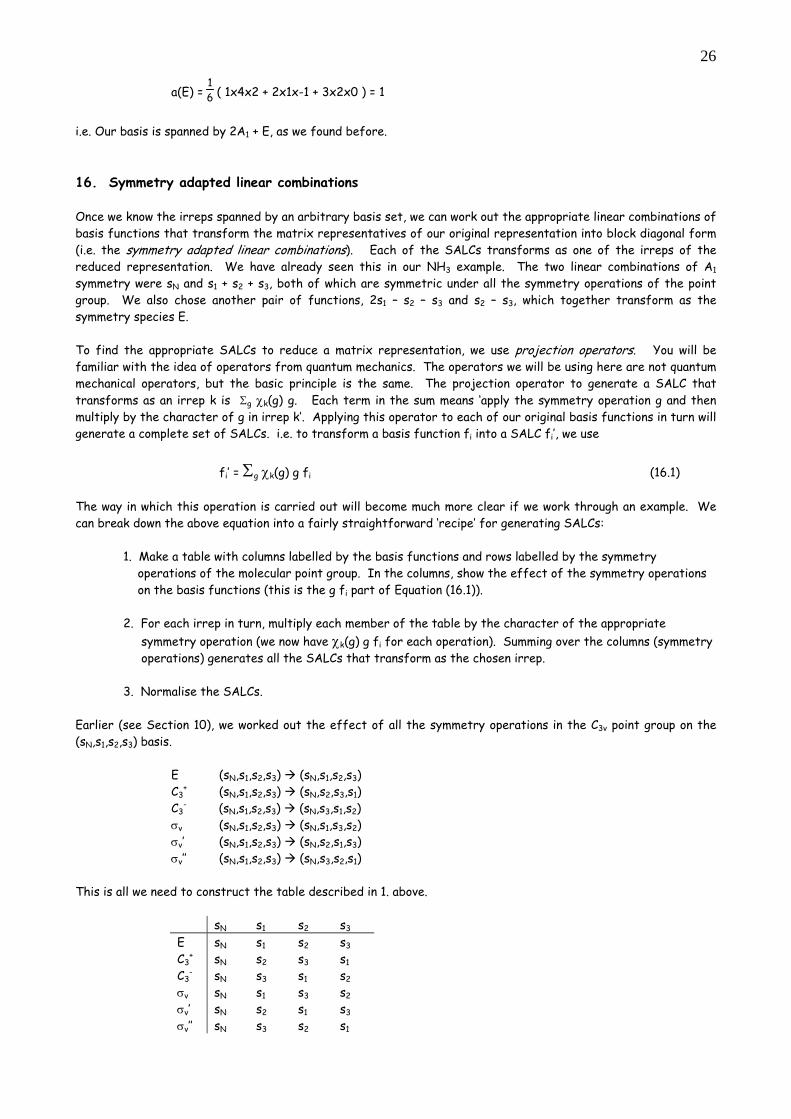
i.e. Our basis is spanned by 2A1 + E, as we found before. 16. Symmetry adapted linear combinations Once we know the irreps spanned by an arbitrary basis set, we can work out the appropriate linear combinations of basis functions that transform the matrix representatives of our original representation into block diagonal form (i.e. the symmetry adapted linear combinations). Each of the SALCs transforms as one of the irreps of the reduced representation. We have already seen this in our NH3 example. The two linear combinations of A1 symmetry were sN and s1 + s2 + s3, both of which are symmetric under all the symmetry operations of the point group. We also chose another pair of functions, 2s1 – s2 – s3 and s2 – s3, which together transform as the symmetry species E. To find the appropriate SALCs to reduce a matrix representation, we use projection operators. You will be familiar with the idea of operators from quantum mechanics. The operators we will be using here are not quantum mechanical operators, but the basic principle is the same. The projection operator to generate a SALC that transforms as an irrep k is Σg χk(g) g. Each term in the sum means ‘apply the symmetry operation g and then multiply by the character of g in irrep k’. Applying this operator to each of our original basis functions in turn will generate a complete set of SALCs. i.e. to transform a basis function fi into a SALC fi’, we use

fi’ = Σg χk(g) g fi (16.1) The way in which this operation is carried out will become much more clear if we work through an example. We can break down the above equation into a fairly straightforward ‘recipe’ for generating SALCs:

1. Make a table with columns labelled by the basis functions and rows labelled by the symmetry operations of the molecular point group. In the columns, show the effect of the symmetry operations on the basis functions (this is the g fi part of Equation (16.1)). 2. For each irrep in turn, multiply each member of the table by the character of the appropriate symmetry operation (we now have χk(g) g fi for each operation). Summing over the columns (symmetry operations) generates all the SALCs that transform as the chosen irrep. 3. Normalise the SALCs.

Earlier (see Section 10), we worked out the effect of all the symmetry operations in the C3v point group on the (sN,s1,s2,s3) basis.

E (sN,s1,s2,s3) (sN,s1,s2,s3) C3

+ (sN,s1,s2,s3) (sN,s2,s3,s1) C3

- (sN,s1,s2,s3) (sN,s3,s1,s2) σv (sN,s1,s2,s3) (sN,s1,s3,s2) σv’ (sN,s1,s2,s3) (sN,s2,s1,s3) σv’’ (sN,s1,s2,s3) (sN,s3,s2,s1)

This is all we need to construct the table described in 1. above.

sN s1 s2 s3 E sN s1 s2 s3 C3

+ sN s2 s3 s1 C3

- sN s3 s1 s2 σv sN s1 s3 s2 σv’ sN s2 s1 s3 σv’’ sN s3 s2 s1

27

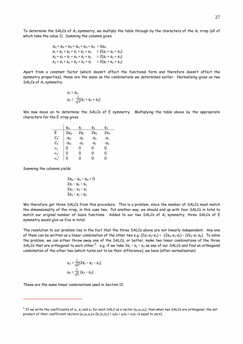
To determine the SALCs of A1 symmetry, we multiply the table through by the characters of the A1 irrep (all of which take the value 1). Summing the columns gives sN + sN + sN + sN + sN + sN = 6sN s1 + s2 + s3 + s1 + s2 + s3 = 2(s1 + s2 + s3) s2 + s3 + s1 + s3 + s1 + s2 = 2(s1 + s2 + s3) s3 + s1 + s2 + s2 + s3 + s1 = 2(s1 + s2 + s3) Apart from a constant factor (which doesn’t affect the functional form and therefore doesn’t affect the symmetry properties), these are the same as the combinations we determined earlier. Normalising gives us two SALCs of A1 symmetry. φ1 = sN

φ2 = 13(s1 + s2 + s3)

We now move on to determine the SALCs of E symmetry. Multiplying the table above by the appropriate characters for the E irrep gives

sN s1 s2 s3 E 2sN 2s1 2s2 2s3 C3

+ -sN -s2 -s3 -s1 C3

- -sN -s3 -s1 -s2 σv 0 0 0 0 σv’ 0 0 0 0 σv’’ 0 0 0 0

Summing the columns yields 2sN – sN – sN = 0 2s1 – s2 – s3 2s2 – s3 – s1 2s3 – s1 – s2 We therefore get three SALCs from this procedure. This is a problem, since the number of SALCs must match the dimensionality of the irrep, in this case two. Put another way, we should end up with four SALCs in total to match our original number of basis functions. Added to our two SALCs of A1 symmetry, three SALCs of E symmetry would give us five in total. The resolution to our problem lies in the fact that the three SALCs above are not linearly independent. Any one of them can be written as a linear combination of the other two e.g. (2s1–s2–s3) = -(2s2-s3-s1) – (2s3-s1-s2). To solve the problem, we can either throw away one of the SALCs, or better, make two linear combinations of the three SALCs that are orthogonal to each other.5 e.g. if we take 2s1 – s2 – s3 as one of our SALCs and find an orthogonal combination of the other two (which turns out to be their difference), we have (after normalisation)

φ3 = 16(2s1 – s2 – s3)

φ4 = 12 (s2 – s3)

These are the same linear combinations used in Section 12.

5 If we write the coefficients of s1, s2 and s3 for each SALC as a vector (a1,a2,a3), then when two SALCs are orthogonal, the dot product of their coefficient vectors (a1,a2,a3) • (b1,b2,b3) = a1b1 + a2b2 + a3b3 is equal to zero).

28

We now have all the machinery we need to apply group theory to a range of chemical problems. In our first application, we will learn how to use molecular symmetry and group theory to help us understand chemical bonding. 17. Determining whether an integral can be non-zero As we continue with this course, we will discover that there are many times when we would like to know whether a particular integral is necessarily zero, or whether there is a chance that it may be non-zero. We can often use group theory to differentiate these two cases. You will have already used symmetry properties of functions to determine whether or not a one-dimensional integral is zero. For example, cos(x) is an ‘even’ function (symmetric with respect to reflection through the origin), and it follows from this that ⌡⌠-∞

∞cos(x) dx = 0 . In general integral between these limits for any other

even function will be also be zero. In the general case we may have an integral of more than one dimension. The key to determining whether a general integral is necessarily zero lies in the fact that because an integral is just a number, it must be invariant to any symmetry operation. For example, bonding in a diatomic (see next section) depends on the presence of a non-zero overlap between atomic orbitals on adjacent atoms, which may be quantified by an overlap integral. You wouldn’t expect the bonding in a molecule to change if you rotated the molecule through some angle θ, so the integral must be invariant to rotation, and indeed to any other symmetry operation. In group theoretical terms, for an integral to be non-zero6, the integrand must transform as the totally symmetric irrep in the appropriate point group. In practice, the integrand may not transform as a single irrep, but it must include the totally symmetric irrep. These ideas should become more clear in the next section. 18. Bonding in diatomics You will already be familiar with the idea of constructing molecular orbitals from linear combinations of atomic orbitals from previous courses covering bonding in diatomic molecules. By considering the symmetries of s and p orbitals on two atoms, we can form bonding and antibonding combinations labelled as having either σ or π symmetry depending on whether they resemble s or a p orbitals when viewed along the bond axis (see diagram below). In all of the cases shown, only atomic orbitals that have the same symmetry when viewed along the bond axis z can form a chemical bond e.g. two s orbitals, two pz orbitals , or an s and a pz can form a bond, but a pz and a px or an s and a px or a py cannot. It turns out that the rule that determines whether or not two atomic orbitals can bond is that they must belong to the same symmetry species within the point group of the molecule. We can prove this mathematically for two atomic orbitals φi and φj by looking at the overlap integral between the two orbitals.

Sij = <φi|φj> = ⌡⌠φi*φj dτ

In order for bonding to be possible, this integral must be non-zero. The product of the two functions φ1 and φ2 transforms as the direct product of their symmetry species i.e. Γ12 = Γ1 ⊗ Γ2. As explained above, for the overlap integral to be non-zero, Γ12 must contain the totally symmetric irrep (A1g for a homonuclear diatomic, which belongs to the point group D∞h). As it happens, this is only possible if φ1 and φ2 belong to the same irrep. These ideas are summarised for a diatomic in the table below. 6 It should be noted that even when the irreps spanned by the integrand do include the totally symmetric irrep, it is still possible for the integral to be zero. All group theory allows us to do is identify integrals that are necessarily zero based on the symmetry (or lack thereof) of the integrand.

29

19. Bonding in polyatomics - constructing molecular orbitals from SALCs In the previous section we showed how to use symmetry to determine whether two atomic orbitals can form a chemical bond. How do we carry out the same procedure for a polyatomic molecule, in which many atomic orbitals may combine to form a bond? Any SALCs of the same symmetry could potentially form a bond, so all we need to do to construct a molecular orbital is take a linear combination of all the SALCs of the same symmetry species. The general procedure is: 1. Use a basis set consisting of valence atomic orbitals on each atom in the system. 2. Determine which irreps are spanned by the basis set and construct the SALCs that transform as each

irrep. 3. Take linear combinations of irreps of the same symmetry species to form the molecular orbitals.

e.g. in our NH3 example we could form a molecular orbital of A1 symmetry from the two SALCs that transform as A1,

Ψ(A1) = c1 φ1 + c2 φ2

= c1sN + c2 13 (s1+s2+s3) (19.1)

Unfortunately, this is as far as group theory can take us. It can give us the functional form of the molecular orbitals but it cannot determine the coefficients c1 and c2. To go further and obtain the expansion coefficients and orbital energies, we must turn to quantum mechanics. The material we are about to cover will be repeated in greater detail in later courses on quantum mechanics and valence, but they are included here to provide you with a complete reference on how to construct molecular orbitals and determine their energies. 20. Calculating the orbital energies and expansion coefficients Note: Sections 20 and 21 are not covered in this lecture course, but the material will be dealt with in other courses (e.g. valence) and is included here for completeness. Calculation of the orbital energies and expansion coefficients is based on the variation principle, which states that any approximate wavefunction must have a higher energy than the true wavefunction. This follows directly from the fairly common-sense idea that in general any system tries to minimize its energy. If an ‘approximate’ wavefunction had a lower energy than the ‘true’ wavefunction, we would expect the system to try and adopt this ‘approximate’ lower energy state, rather than the ‘true’ state. That all approximations to the true wavefunction must have a higher energy than the true wavefunction is the only scenario that makes physical sense. A mathematical proof of the variation principle is given in the Appendix. We apply the variation principle as follows:

First atomic orbital

Second atomic orbital

Γ1 ⊗ Γ2 Overlap integral

Bonding?

s (A1g) s (A1g) A1g Non-zero Yes s (A1g) px (E1u) E1u Zero No s (A1g) pz (A1u) A1u Zero No px (E1u) px (E1u) A1g + A2g + E2g Non-zero Yes px (E1u) pz (A1u) E1g Zero No pz (A1u) pz (A1u) A1g Non-zero Yes

30

Molecular energy levels, or orbital energies, are eigenvalues of the molecular Hamiltonian H. Using a standard result from quantum mechanics, it follows that the energy E of a molecular orbital Ψ is

E = <Ψ|H|Ψ>

<Ψ|Ψ> (unnormalised Ψ) (20.1)

or E = <Ψ|H|Ψ> (normalised Ψ, for which <Ψ|Ψ> = 1) (20.2)

If the true wavefunction has the lowest energy, then to find the closest approximation we can to the true wavefunction, all we have to do is find the coefficients in our expansion of SALCs that minimise the energy in the above expressions. In practice, we substitute our wavefunction into Equation (19.1) and minimise the resulting expression with respect to the coefficients. To show how this is done, we’ll use our NH3 wavefunction of A1 symmetry from the previous section. Substituting into Equation (20.1) gives:

E = <c1φ1+c2φ2|H|c1φ1+c2φ2>< c1φ1+c2φ2| c1φ1+c2φ2>

= <c1φ1|H|c1φ1> + <c1φ1|H|c2φ2> + <c2φ2|H|c1φ1> + <c2φ2|H|c2φ2>

<c1φ1|c1φ1> + <c1φ1|c2φ2> + <c2φ2|c1φ1> + <c2φ2|c2φ2>

= c1

2<φ1|H|φ1> + c1c2<φ1|H|φ2> + c2c1<φ2|H|φ1> + c22<φ2|H|φ2>

c12<φ1|φ1> + c1c2<φ1|φ2> + c2c1<φ2|φ1> + c2

2<φ2|φ2>

If we now define a Hamiltonian matrix element Hij = <φi|H|φj> and an overlap integral Sij = <φi|φj> and note that Hij=Hji and Sij = Sji, this simplifies to

E = c1

2H11 + 2c1c2H12 + c22H22

c12S11 + 2c1c2S12 + c2

2S22

To get this into a simpler form for carrying out the energy minimisation, we multiply both sides through by the denominator to give E (c1

2S11 + 2c1c2S12 + c22S22) = c1

2H11 + 2c1c2H12 + c22H22

Now we need to minimise the energy with respect to c1 and c2 i.e. we require ∂E∂c1

= 0 and ∂E∂c2

= 0. If we

differentiate the above equation through separately by c1 and c2 and apply this condition, we will end up with two equations in the two unknowns c1 and c2, which we can solve to determine the coefficients and the energy. Differentiating by c1 gives

∂E∂c1

( c12S11 + 2c1c2S12 + c2

2S22) + E(2c1S11 + 2c2S12) = 2c1H11 + 2c2H12

Differentiating by c2 gives

∂E∂c2

( c12S11 + 2c1c2S12 + c2

2S22) + E(2c1S12 + 2c2S22) = 2c1H12 + 2c2H22

Because ∂E∂c1

= ∂E∂c2

= 0, the first term on the left hand side of both equations is zero, leaving us with

E(2c1S11 + 2c2S12) = 2c1H11 + 2c2H12 E(2c1S12 + 2c2S22) = 2c1H12 + 2c2H22

These are normally rewritten slightly, in the form

31

c1(H11-ES11) + c2(H12-ES12) = 0 (20.3) c1(H12-ES12) + c2(H22-ES22) = 0 These equations are known as the secular equations and are the set of equations we need to solve to determine c1, c2 and E. In the general case (derived in the Appendix), when our wavefunction is a linear combination of N SALCs (i.e. Ψ =∑i=1

N ci φi) we get N equations in N unknowns, with the kth equation given by

∑i=1

N ci(Hki–ESki) = 0 (20.4)

Note that we can use any basis functions we like together with the linear variation method described here to construct approximate molecular orbitals and determine their energies, but choosing to use SALCs simplifies things considerably when the number of basis functions is large. An arbitrary set of N basis functions leads to a set of N equations in N unknowns, which must be solved simultaneously. Converting the basis into a set of SALCs separates the equations into several smaller sets of secular equations, one for each irrep, which can be solved independently. It is usually easier to solve several sets of secular equations of lower dimensionality than one set of higher dimensionality. 21. Solving the secular equations 21.1 Matrix formulation of a set of linear equations As we have seen already, any set of linear equations may be rewritten as a matrix equation Ax = b. Linear equations are classified as simultaneous linear equations or homogeneous linear equations, depending on whether the vector b on the RHS of the equation is non-zero or zero. For a set of simultaneous linear equations (non-zero b) it is fairly apparent that if a unique solution exists, it can be found by multiplying both sides by the inverse matrix A-1 (since A-1A on the left hand side is equal to the identity matrix, which has no effect on the vector x) Ax = b A-1Ax = A-1b x = A-1b In practice, there are easier matrix methods for solving simultaneous equations than finding the inverse matrix, but these need not concern us here. In Section 8.4, we discovered that in order for a matrix to have an inverse, it must have a non-zero determinant. Since A-1 must exist in order for a set of simultaneous linear equations to have a solution, this means that the determinant of the matrix A must be non-zero for the equations to be solvable. The reverse is true for homogeneous linear equations. In this case the set of equations only has a solution if the determinant of A is equal to zero. The secular equations we want to solve are homogeneous equations, and we will use this property of the determinant to determine the molecular orbital energies. An important property of homogeneous equations is that if a vector x is a solution, so is any multiple of x, meaning that the solutions (the molecular orbitals) can be normalised without causing any problems. 21.2 Solving for the orbital energies and expansion coefficients Recall the secular equations for the A1 orbitals of NH3 derived in the previous section c1(H11-ES11) + c2(H12-ES12) = 0 c1(H12-ES12) + c2(H22-ES22) = 0

32

where c1 and c2 are the coefficients in the linear combination of the SALCs φ1 = sN and φ2 = 13 (s1 + s2 + s3) used to

construct the molecular orbital. Writing this set of homogeneous linear equations in matrix form gives

⎝⎛

⎠⎞H11-ES11 H12-ES12

H12-ES12 H22-ES22 ⎝⎛

⎠⎞c1

c2 = ⎝

⎛⎠⎞0

0 (21.2.1)

In order for the equations to have a solution, the determinant of the matrix must be equal to zero. Writing out the determinant will give us a polynomial equation in E that we can solve to obtain the orbital energies in terms of the Hamiltonian matrix elements Hij and overlap integrals Sij. The number of energies obtained by ‘solving the secular determinant’ in this way is equal to the order of the matrix, in this case two. The secular determinant for Equation (21.2.1) is (noting that S11 = S22 = 1 since the SALCs are normalised) (H11-E)(H22-E) - (H12-ES12)2 = 0 Expanding and collecting terms in E gives E2(1-S12

2) + E(2H12S12-H11-H22) + (H11H22-H122) = 0

which can be solved using the quadratic formula to give the energies of the two molecular orbitals.

E± = -(2H12S12-H11-H22) ± (2H12S12-H11-H22)2 - 4(1-S12

2)(H11H22-H122)

2(1-S122) (21.2.2)

To obtain numerical values for the energies, we need to evaluate the integrals H11, H22, H12, S12. This would be quite a challenge to do analytically, but luckily there are a number of computer programs that can be used to calculate the integrals. One such program gives the following values.

H11 = -26.0000 eV H22 = -22.2216 eV H12 = -29.7670 eV S12 = 0.8167

When we substitute these into our equation for the energy levels, we get: E+ = 29.8336 eV

E- = -31.0063 eV We now have the orbital energies. The next step is to find the orbital coefficients. The coefficients for an orbital of energy E are found by substituting the energy into the secular equations and solving for the coefficients ci. Since the two secular equations are not linearly independent (i.e. they are effectively only one equation), when we solve them to find the coefficients what we will end up with is the relative values of the coefficients. This is true in general: in a system with N coefficients, solving the secular equations will allow all N of the coefficients ci to be obtained in terms of, say, c1. The absolute values of the coefficients are found by normalising the wavefunction. Since the secular equations for the orbitals of energy E+ and E- are not linearly independent, we can choose to solve either one of them to find the orbital coefficients. We will choose the first.

(H11- E±)c1 + (H12- E±S12)c2 = 0

For the orbital with energy E- = -31.0063 eV, substituting numerical values into this equation gives 5.0063 c1 – 4.4442 c2 = 0 c2 = 1.1265 c1

33

The molecular orbital is therefore

ψ1 = c1(φ1 +1.1265 φ2) Normalising to find the constant c1 (by requiring <ψ|ψ> = 1) gives ψ1 = 0.4933 φ1 + 0.5557 φ2 = 0.4933 sN + 0.3208 (s1 + s2 + s3) (substituting the SALCs for φ1 and φ2)

For the second orbital, with energy E+ = 29.8336 eV, the secular equation is -55.8336 c1 – 54.1321 c2 = 0 c2 = -1.0314 c1 giving

ψ2 = c1(φ1 – 1.0314 φ2) = 1.6242 φ1 – 1.6752 φ2 (after normalisation) = 1.6242 sN – 0.9672 (s1 + s2 + s3) These two A1 molecular orbitals ψ1 and ψ2, one bonding and one antibonding, are shown below.

Ψ1 Ψ2 The remaining two SALCs arising from the s orbitals of NH3 (φ3 =

1

6(2s1–s2 –s3) and φ4 = 1

2(s2–s3)), form an

orthogonal pair of molecular orbitals of E symmetry. We can show this by solving the secular determinant to find the orbital energies. The secular equations in this case are: Solving the secular determinant gives

E± = -(2H34S34-H33-H44) ± (2H34S34-H33-H44)2 - 4(1-S34

2)(H33H44-H342)

2(1-S342)

The integrals required are H33 = -9.2892 eV H44 = -9.2892 eV H34 = 0 S34 = 0 Using the fact that H34 = S34 = 0, the expression for the energies reduces to

E± = (H33+H44) ± (H33-H44)

2

giving E+ = H33 = -9.2892 eV and E- = H44 = -9.2892 eV. Each SALC therefore forms a molecular orbital by itself, and the two orbitals have the same energy; the two SALCs form an orthogonal pair of degenerate orbitals. These two molecular orbitals of E symmetry are shown below.

Ψ 3 ψ4

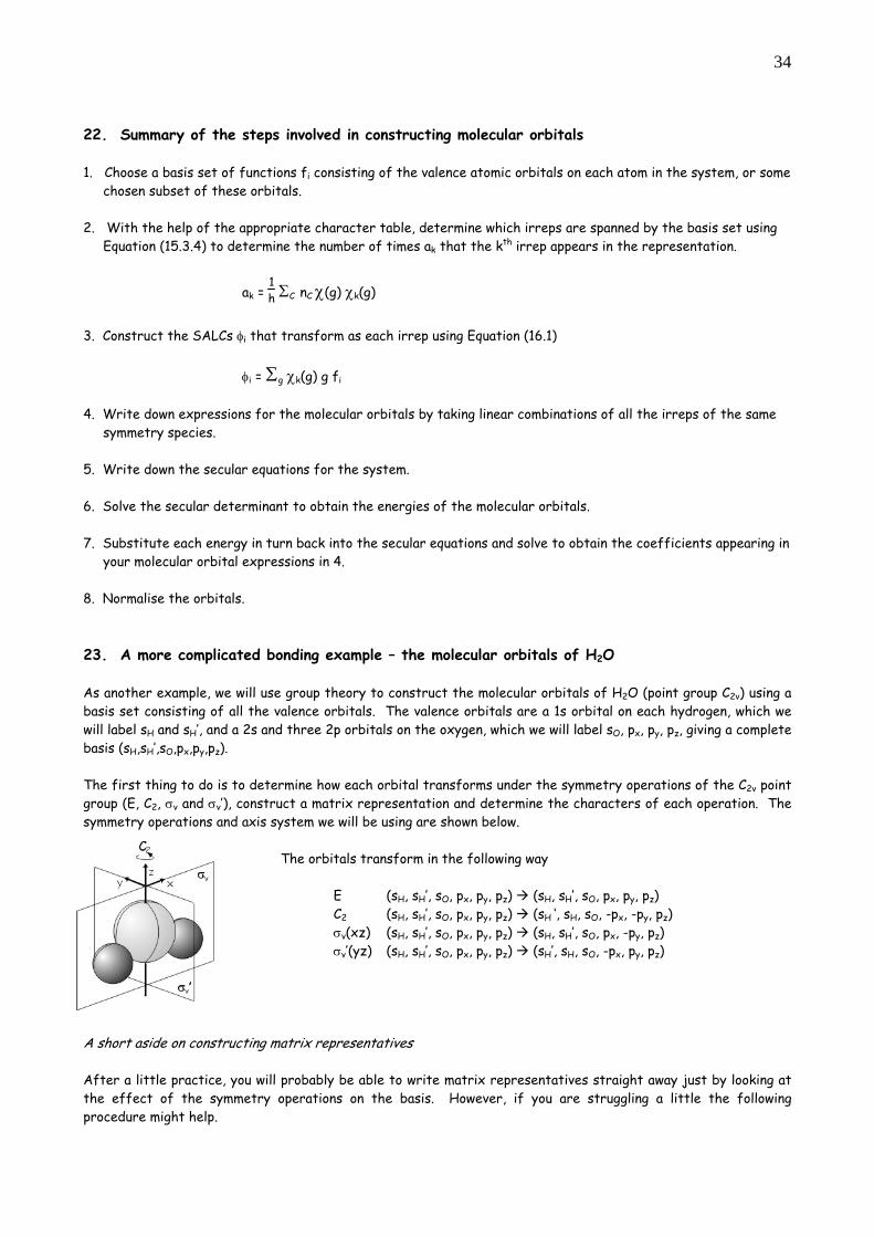
34

22. Summary of the steps involved in constructing molecular orbitals 1. Choose a basis set of functions fi consisting of the valence atomic orbitals on each atom in the system, or some chosen subset of these orbitals. 2. With the help of the appropriate character table, determine which irreps are spanned by the basis set using Equation (15.3.4) to determine the number of times ak that the kth irrep appears in the representation.

ak = 1h ΣC nC χ(g) χk(g)

3. Construct the SALCs φi that transform as each irrep using Equation (16.1)

φi = Σg χk(g) g fi

4. Write down expressions for the molecular orbitals by taking linear combinations of all the irreps of the same symmetry species. 5. Write down the secular equations for the system. 6. Solve the secular determinant to obtain the energies of the molecular orbitals. 7. Substitute each energy in turn back into the secular equations and solve to obtain the coefficients appearing in your molecular orbital expressions in 4. 8. Normalise the orbitals. 23. A more complicated bonding example – the molecular orbitals of H2O As another example, we will use group theory to construct the molecular orbitals of H2O (point group C2v) using a basis set consisting of all the valence orbitals. The valence orbitals are a 1s orbital on each hydrogen, which we will label sH and sH’, and a 2s and three 2p orbitals on the oxygen, which we will label sO, px, py, pz, giving a complete basis (sH,sH’,sO,px,py,pz). The first thing to do is to determine how each orbital transforms under the symmetry operations of the C2v point group (E, C2, σv and σv’), construct a matrix representation and determine the characters of each operation. The symmetry operations and axis system we will be using are shown below.

The orbitals transform in the following way E (sH, sH’, sO, px, py, pz) (sH, sH’, sO, px, py, pz) C2 (sH, sH’, sO, px, py, pz) (sH

‘, sH, sO, -px, -py, pz) σv(xz) (sH, sH’, sO, px, py, pz) (sH, sH’, sO, px, -py, pz) σv’(yz) (sH, sH’, sO, px, py, pz) (sH’, sH, sO, -px, py, pz)

A short aside on constructing matrix representatives After a little practice, you will probably be able to write matrix representatives straight away just by looking at the effect of the symmetry operations on the basis. However, if you are struggling a little the following procedure might help.

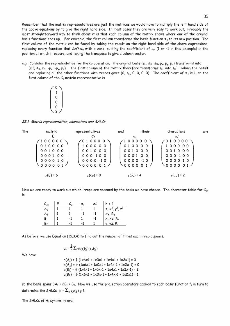
35

Remember that the matrix representatives are just the matrices we would have to multiply the left hand side of the above equations by to give the right hand side. In most cases they are very easy to work out. Probably the most straightforward way to think about it is that each column of the matrix shows where one of the original basis functions ends up. For example, the first column transforms the basis function sH to its new position. The first column of the matrix can be found by taking the result on the right hand side of the above expressions, replacing every function that isn’t sH with a zero, putting the coefficient of sH (1 or –1 in this example) in the position at which it occurs, and taking the transpose to give a column vector. e.g. Consider the representative for the C2 operation. The original basis (sH, sH’, sO, px, py, pz) transforms into

(sH’, sH, sO, -px, -py, pz). The first column of the matrix therefore transforms sH into sH’. Taking the result and replacing all the other functions with zeroes gives (0, sH, 0, 0, 0, 0). The coefficient of sH is 1, so the first column of the C2 matrix representative is

⎝⎜⎛

⎠⎟⎞

0 1 0 0 0 0

23.1 Matrix representation, characters and SALCs The matrix representatives and their characters are E C2 σv σv’

⎝⎜⎛

⎠⎟⎞

1 0 0 0 0 0 0 1 0 0 0 0 0 0 1 0 0 0 0 0 0 1 0 0 0 0 0 0 1 0 0 0 0 0 0 1

⎝⎜⎛

⎠⎟⎞

0 1 0 0 0 0 1 0 0 0 0 0 0 0 1 0 0 0 0 0 0 -1 0 0 0 0 0 0 -1 0 0 0 0 0 0 1

⎝⎜⎛

⎠⎟⎞

1 0 0 0 0 0 0 1 0 0 0 0 0 0 1 0 0 0 0 0 0 1 0 0 0 0 0 0 -1 0 0 0 0 0 0 1

⎝⎜⎛

⎠⎟⎞

0 1 0 0 0 0 1 0 0 0 0 0 0 0 1 0 0 0 0 0 0 -1 0 0 0 0 0 0 1 0 0 0 0 0 0 1

χ(E) = 6 χ(C2) = 0 χ(σv) = 4 χ(σv’) = 2

Now we are ready to work out which irreps are spanned by the basis we have chosen. The character table for C2v

is: As before, we use Equation (15.3.4) to find out the number of times each irrep appears.

ak = 1h ΣC nCχ(g) χk(g)

We have a(A1) = ¼ (1x6x1 + 1x0x1 + 1x4x1 + 1x2x1) = 3

a(A2) = ¼ (1x6x1 + 1x0x1 + 1x4x-1 + 1x2x-1) = 0 a(B1) = ¼ (1x6x1 + 1x0x-1 + 1x4x1 + 1x2x-1) = 2 a(B2) = ¼ (1x6x1 + 1x0x-1 + 1x4x-1 + 1x2x1) = 1 so the basis spans 3A1 + 2B1 + B2. Now we use the projection operators applied to each basis function fi in turn to

determine the SALCs φi = Σg χk(g) g fi The SALCs of A1 symmetry are:

C2v E C2 σv σv’ h = 4 A1 1 1 1 1 z, x2, y2, z2 A2 1 1 -1 -1 xy, Rz B1 1 -1 1 -1 x, xz, Ry B2 1 -1 -1 1 y, yz, Rx

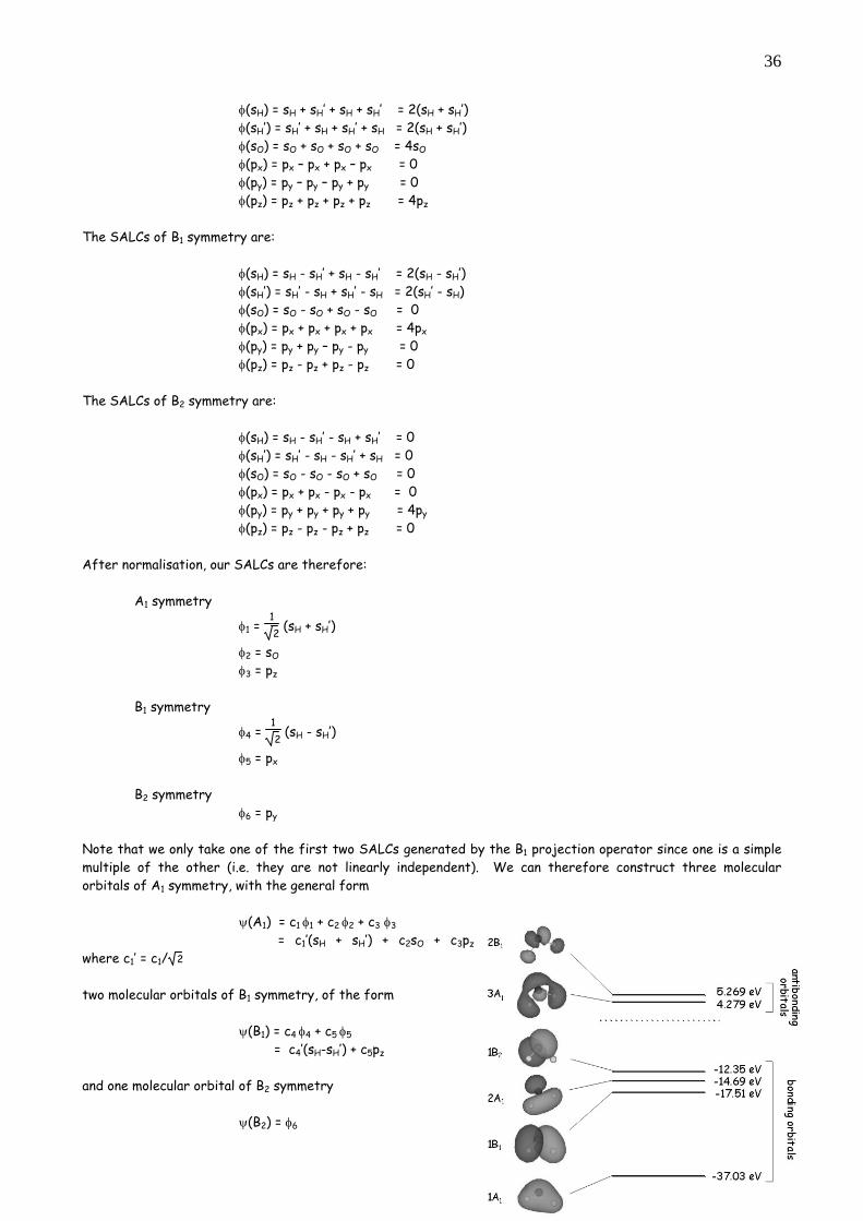
36

φ(sH) = sH + sH’ + sH + sH’ = 2(sH + sH’) φ(sH’) = sH’ + sH + sH’ + sH = 2(sH + sH’) φ(sO) = sO + sO + sO + sO = 4sO φ(px) = px – px + px – px = 0 φ(py) = py – py – py + py = 0 φ(pz) = pz + pz + pz + pz = 4pz The SALCs of B1 symmetry are: φ(sH) = sH - sH’ + sH - sH’ = 2(sH - sH’) φ(sH’) = sH’ - sH + sH’ - sH = 2(sH’ - sH) φ(sO) = sO - sO + sO - sO = 0 φ(px) = px + px + px + px = 4px φ(py) = py + py – py - py = 0 φ(pz) = pz - pz + pz - pz = 0 The SALCs of B2 symmetry are: φ(sH) = sH - sH’ - sH + sH’ = 0 φ(sH’) = sH’ - sH - sH’ + sH = 0 φ(sO) = sO - sO - sO + sO = 0 φ(px) = px + px - px - px = 0 φ(py) = py + py + py + py = 4py φ(pz) = pz - pz - pz + pz = 0 After normalisation, our SALCs are therefore: A1 symmetry

φ1 = 12 (sH + sH’)

φ2 = sO φ3 = pz B1 symmetry

φ4 = 12 (sH - sH’)

φ5 = px B2 symmetry φ6 = py Note that we only take one of the first two SALCs generated by the B1 projection operator since one is a simple multiple of the other (i.e. they are not linearly independent). We can therefore construct three molecular orbitals of A1 symmetry, with the general form

ψ(A1) = c1 φ1 + c2 φ2 + c3 φ3 = c1’(sH + sH’) + c2sO + c3pz

where c1’ = c1/ 2 two molecular orbitals of B1 symmetry, of the form ψ(B1) = c4 φ4 + c5 φ5 = c4’(sH-sH’) + c5pz and one molecular orbital of B2 symmetry

ψ(B2) = φ6

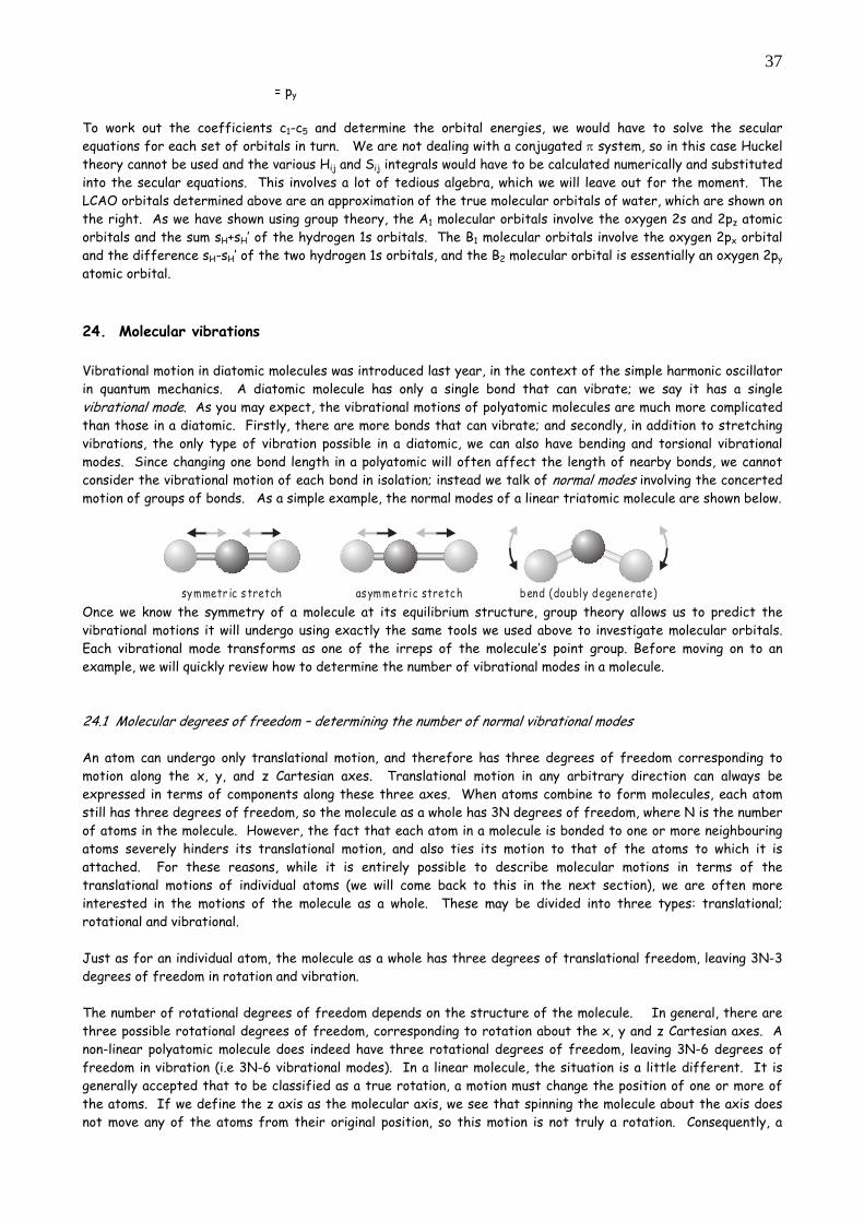
37

= py To work out the coefficients c1-c5 and determine the orbital energies, we would have to solve the secular equations for each set of orbitals in turn. We are not dealing with a conjugated π system, so in this case Huckel theory cannot be used and the various Hij and Sij integrals would have to be calculated numerically and substituted into the secular equations. This involves a lot of tedious algebra, which we will leave out for the moment. The LCAO orbitals determined above are an approximation of the true molecular orbitals of water, which are shown on the right. As we have shown using group theory, the A1 molecular orbitals involve the oxygen 2s and 2pz atomic orbitals and the sum sH+sH’ of the hydrogen 1s orbitals. The B1 molecular orbitals involve the oxygen 2px orbital and the difference sH-sH’ of the two hydrogen 1s orbitals, and the B2 molecular orbital is essentially an oxygen 2py atomic orbital. 24. Molecular vibrations Vibrational motion in diatomic molecules was introduced last year, in the context of the simple harmonic oscillator in quantum mechanics. A diatomic molecule has only a single bond that can vibrate; we say it has a single vibrational mode. As you may expect, the vibrational motions of polyatomic molecules are much more complicated than those in a diatomic. Firstly, there are more bonds that can vibrate; and secondly, in addition to stretching vibrations, the only type of vibration possible in a diatomic, we can also have bending and torsional vibrational modes. Since changing one bond length in a polyatomic will often affect the length of nearby bonds, we cannot consider the vibrational motion of each bond in isolation; instead we talk of normal modes involving the concerted motion of groups of bonds. As a simple example, the normal modes of a linear triatomic molecule are shown below.

symmetr ic s tretch asymmetric stretch bend (doubly degenerate) Once we know the symmetry of a molecule at its equilibrium structure, group theory allows us to predict the vibrational motions it will undergo using exactly the same tools we used above to investigate molecular orbitals. Each vibrational mode transforms as one of the irreps of the molecule’s point group. Before moving on to an example, we will quickly review how to determine the number of vibrational modes in a molecule. 24.1 Molecular degrees of freedom – determining the number of normal vibrational modes An atom can undergo only translational motion, and therefore has three degrees of freedom corresponding to motion along the x, y, and z Cartesian axes. Translational motion in any arbitrary direction can always be expressed in terms of components along these three axes. When atoms combine to form molecules, each atom still has three degrees of freedom, so the molecule as a whole has 3N degrees of freedom, where N is the number of atoms in the molecule. However, the fact that each atom in a molecule is bonded to one or more neighbouring atoms severely hinders its translational motion, and also ties its motion to that of the atoms to which it is attached. For these reasons, while it is entirely possible to describe molecular motions in terms of the translational motions of individual atoms (we will come back to this in the next section), we are often more interested in the motions of the molecule as a whole. These may be divided into three types: translational; rotational and vibrational. Just as for an individual atom, the molecule as a whole has three degrees of translational freedom, leaving 3N-3 degrees of freedom in rotation and vibration. The number of rotational degrees of freedom depends on the structure of the molecule. In general, there are three possible rotational degrees of freedom, corresponding to rotation about the x, y and z Cartesian axes. A non-linear polyatomic molecule does indeed have three rotational degrees of freedom, leaving 3N-6 degrees of freedom in vibration (i.e 3N-6 vibrational modes). In a linear molecule, the situation is a little different. It is generally accepted that to be classified as a true rotation, a motion must change the position of one or more of the atoms. If we define the z axis as the molecular axis, we see that spinning the molecule about the axis does not move any of the atoms from their original position, so this motion is not truly a rotation. Consequently, a

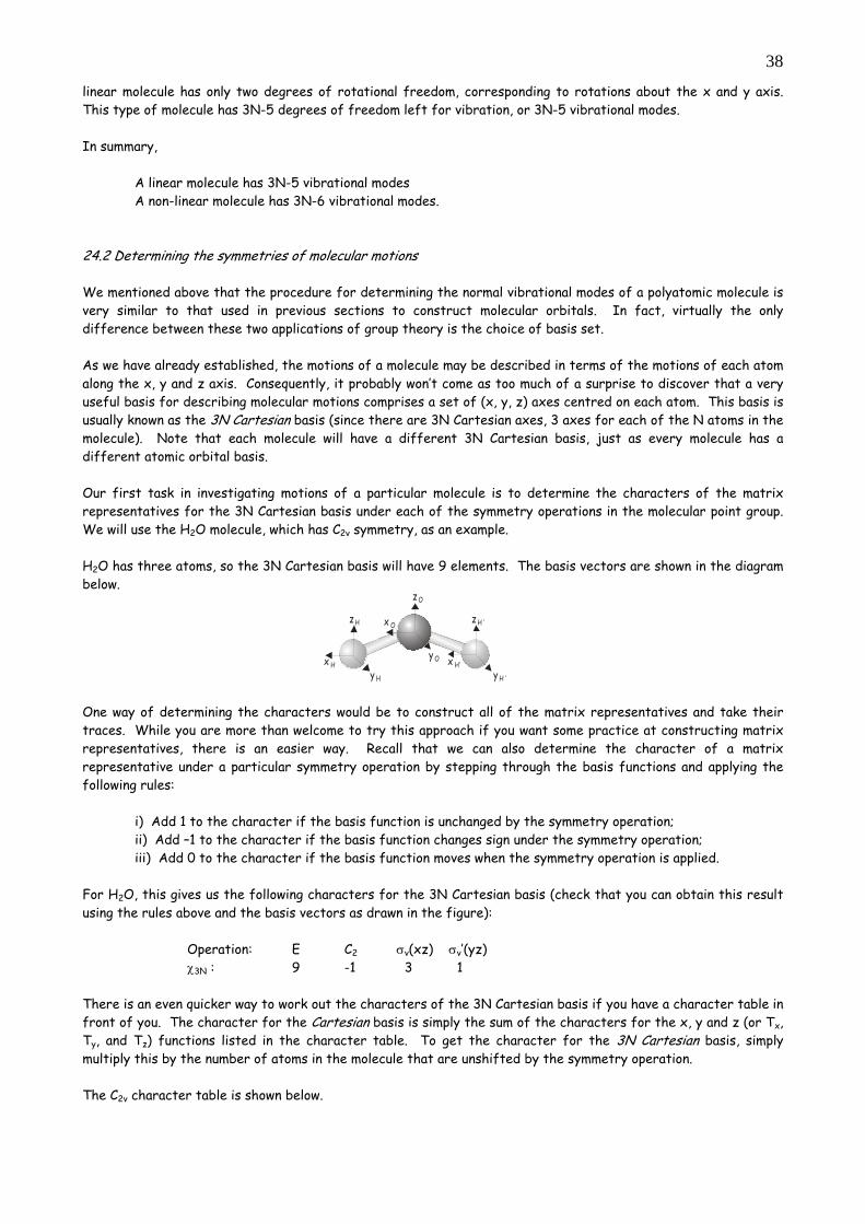
38

linear molecule has only two degrees of rotational freedom, corresponding to rotations about the x and y axis. This type of molecule has 3N-5 degrees of freedom left for vibration, or 3N-5 vibrational modes. In summary, A linear molecule has 3N-5 vibrational modes A non-linear molecule has 3N-6 vibrational modes. 24.2 Determining the symmetries of molecular motions We mentioned above that the procedure for determining the normal vibrational modes of a polyatomic molecule is very similar to that used in previous sections to construct molecular orbitals. In fact, virtually the only difference between these two applications of group theory is the choice of basis set. As we have already established, the motions of a molecule may be described in terms of the motions of each atom along the x, y and z axis. Consequently, it probably won’t come as too much of a surprise to discover that a very useful basis for describing molecular motions comprises a set of (x, y, z) axes centred on each atom. This basis is usually known as the 3N Cartesian basis (since there are 3N Cartesian axes, 3 axes for each of the N atoms in the molecule). Note that each molecule will have a different 3N Cartesian basis, just as every molecule has a different atomic orbital basis. Our first task in investigating motions of a particular molecule is to determine the characters of the matrix representatives for the 3N Cartesian basis under each of the symmetry operations in the molecular point group. We will use the H2O molecule, which has C2v symmetry, as an example. H2O has three atoms, so the 3N Cartesian basis will have 9 elements. The basis vectors are shown in the diagram below.

x H

y H

x H’y H ’

z H ’x O

y O

zO

zH

One way of determining the characters would be to construct all of the matrix representatives and take their traces. While you are more than welcome to try this approach if you want some practice at constructing matrix representatives, there is an easier way. Recall that we can also determine the character of a matrix representative under a particular symmetry operation by stepping through the basis functions and applying the following rules: i) Add 1 to the character if the basis function is unchanged by the symmetry operation; ii) Add –1 to the character if the basis function changes sign under the symmetry operation; iii) Add 0 to the character if the basis function moves when the symmetry operation is applied. For H2O, this gives us the following characters for the 3N Cartesian basis (check that you can obtain this result using the rules above and the basis vectors as drawn in the figure): Operation: E C2 σv(xz) σv’(yz) χ3N : 9 -1 3 1 There is an even quicker way to work out the characters of the 3N Cartesian basis if you have a character table in front of you. The character for the Cartesian basis is simply the sum of the characters for the x, y and z (or Tx, Ty, and Tz) functions listed in the character table. To get the character for the 3N Cartesian basis, simply multiply this by the number of atoms in the molecule that are unshifted by the symmetry operation. The C2v character table is shown below.

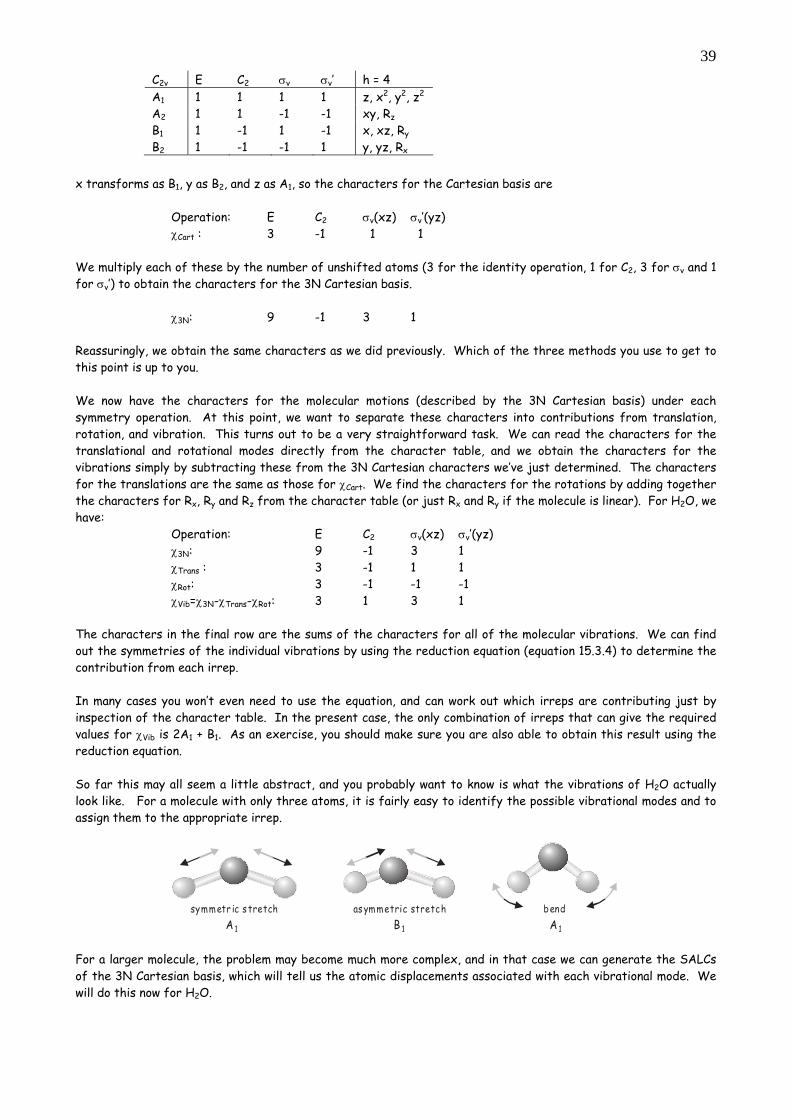
39

x transforms as B1, y as B2, and z as A1, so the characters for the Cartesian basis are Operation: E C2 σv(xz) σv’(yz) χCart : 3 -1 1 1 We multiply each of these by the number of unshifted atoms (3 for the identity operation, 1 for C2, 3 for σv and 1 for σv’) to obtain the characters for the 3N Cartesian basis. χ3N: 9 -1 3 1 Reassuringly, we obtain the same characters as we did previously. Which of the three methods you use to get to this point is up to you. We now have the characters for the molecular motions (described by the 3N Cartesian basis) under each symmetry operation. At this point, we want to separate these characters into contributions from translation, rotation, and vibration. This turns out to be a very straightforward task. We can read the characters for the translational and rotational modes directly from the character table, and we obtain the characters for the vibrations simply by subtracting these from the 3N Cartesian characters we’ve just determined. The characters for the translations are the same as those for χCart. We find the characters for the rotations by adding together the characters for Rx, Ry and Rz from the character table (or just Rx and Ry if the molecule is linear). For H2O, we have: Operation: E C2 σv(xz) σv’(yz)

χ3N: 9 -1 3 1 χTrans : 3 -1 1 1

χRot: 3 -1 -1 -1 χVib=χ3N-χTrans-χRot: 3 1 3 1 The characters in the final row are the sums of the characters for all of the molecular vibrations. We can find out the symmetries of the individual vibrations by using the reduction equation (equation 15.3.4) to determine the contribution from each irrep. In many cases you won’t even need to use the equation, and can work out which irreps are contributing just by inspection of the character table. In the present case, the only combination of irreps that can give the required values for χVib is 2A1 + B1. As an exercise, you should make sure you are also able to obtain this result using the reduction equation. So far this may all seem a little abstract, and you probably want to know is what the vibrations of H2O actually look like. For a molecule with only three atoms, it is fairly easy to identify the possible vibrational modes and to assign them to the appropriate irrep.

A1 B 1 A1

symmetr ic s tretch as ymmetric stretch bend

For a larger molecule, the problem may become much more complex, and in that case we can generate the SALCs of the 3N Cartesian basis, which will tell us the atomic displacements associated with each vibrational mode. We will do this now for H2O.

C2v E C2 σv σv’ h = 4 A1 1 1 1 1 z, x2, y2, z2 A2 1 1 -1 -1 xy, Rz B1 1 -1 1 -1 x, xz, Ry B2 1 -1 -1 1 y, yz, Rx

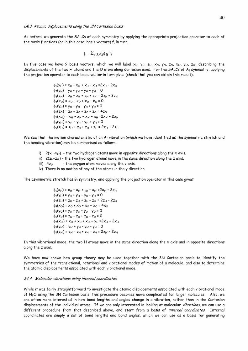
40

24.3 Atomic displacements using the 3N Cartesian basis As before, we generate the SALCs of each symmetry by applying the appropriate projection operator to each of the basis functions (or in this case, basis vectors) fi in turn.

φi = Σg χk(g) g fi In this case we have 9 basis vectors, which we will label xH, yH, zH, xO, yO, zO, xH’, yH’, zH’, describing the displacements of the two H atoms and the O atom along Cartesian axes. For the SALCs of A1 symmetry, applying the projection operator to each basis vector in turn gives (check that you can obtain this result): φ1(xH) = xH – xH’ + xH – xH’ =2xH – 2xH’ φ2(yH) = yH – yH’ – yH + yH’ = 0 φ3(zH) = zH + zH’ + zH + zH’ = 2zH + 2zH’ φ4(xO) = xO – xO + xO – xO = 0 φ5(yO) = yO – yO – yO + yO = 0 φ6(zO) = zO + zO + zO + zO = 4zO

φ7(xH’) = xH’ – xH + xH’ – xH =2xH’ – 2xH φ8(yH’) = yH’ – yH – yH’ + yH = 0 φ9(zH’) = zH’ + zH + zH’ + zH = 2zH’ + 2zH We see that the motion characteristic of an A1 vibration (which we have identified as the symmetric stretch and the bending vibration) may be summarised as follows: i) 2(xH-xH’) - the two hydrogen atoms move in opposite directions along the x axis. ii) 2(zH+zH’) – the two hydrogen atoms move in the same direction along the z axis. iii) 4zO - the oxygen atom moves along the z axis.

iv) There is no motion of any of the atoms in the y direction. The asymmetric stretch has B1 symmetry, and applying the projection operator in this case gives: φ1(xH) = xH + xH’ + xH + xH’ =2xH + 2xH’ φ2(yH) = yH + yH’ – yH - yH’ = 0 φ3(zH) = zH - zH’ + zH - zH’ = 2zH – 2zH’ φ4(xO) = xO + xO + xO + xO = 4xO φ5(yO) = yO + yO – yO - yO = 0 φ6(zO) = zO - zO + zO - zO = 0

φ7(xH’) = xH’ + xH + xH’ + xH =2xH’ + 2xH φ8(yH’) = yH’ + yH – yH’ - yH = 0 φ9(zH’) = zH’ - zH + zH’ - zH = 2zH’ – 2zH In this vibrational mode, the two H atoms move in the same direction along the x axis and in opposite directions along the z axis. We have now shown how group theory may be used together with the 3N Cartesian basis to identify the symmetries of the translational, rotational and vibrational modes of motion of a molecule, and also to determine the atomic displacements associated with each vibrational mode. 24.4 Molecular vibrations using internal coordinates While it was fairly straightforward to investigate the atomic displacements associated with each vibrational mode of H2O using the 3N Cartesian basis, this procedure becomes more complicated for larger molecules. Also, we are often more interested in how bond lengths and angles change in a vibration, rather than in the Cartesian displacements of the individual atoms. If we are only interested in looking at molecular vibrations, we can use a different procedure from that described above, and start from a basis of internal coordinates. Internal coordinates are simply a set of bond lengths and bond angles, which we can use as a basis for generating

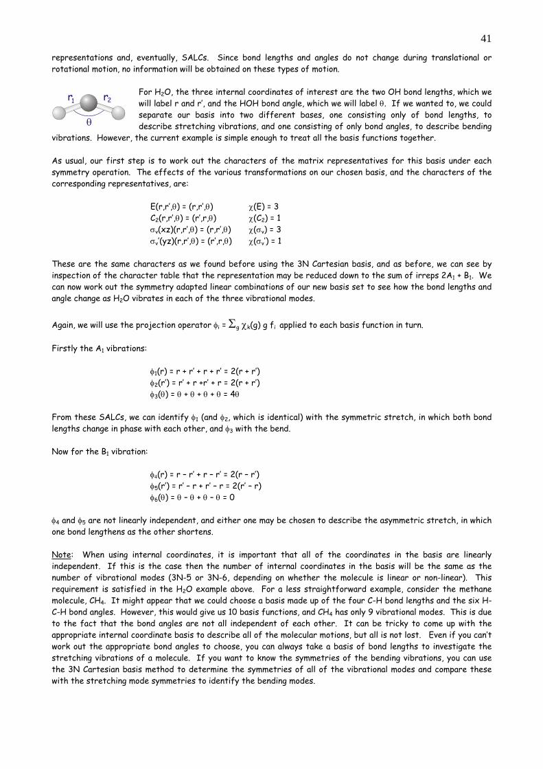
41

representations and, eventually, SALCs. Since bond lengths and angles do not change during translational or rotational motion, no information will be obtained on these types of motion.

For H2O, the three internal coordinates of interest are the two OH bond lengths, which we will label r and r’, and the HOH bond angle, which we will label θ. If we wanted to, we could separate our basis into two different bases, one consisting only of bond lengths, to describe stretching vibrations, and one consisting of only bond angles, to describe bending

vibrations. However, the current example is simple enough to treat all the basis functions together. As usual, our first step is to work out the characters of the matrix representatives for this basis under each symmetry operation. The effects of the various transformations on our chosen basis, and the characters of the corresponding representatives, are: E(r,r’,θ) = (r,r’,θ) χ(E) = 3 C2(r,r’,θ) = (r’,r,θ) χ(C2) = 1 σv(xz)(r,r’,θ) = (r,r’,θ) χ(σv) = 3 σv’(yz)(r,r’,θ) = (r’,r,θ) χ(σv’) = 1 These are the same characters as we found before using the 3N Cartesian basis, and as before, we can see by inspection of the character table that the representation may be reduced down to the sum of irreps 2A1 + B1. We can now work out the symmetry adapted linear combinations of our new basis set to see how the bond lengths and angle change as H2O vibrates in each of the three vibrational modes.

Again, we will use the projection operator φi = Σg χk(g) g fi applied to each basis function in turn. Firstly the A1 vibrations: φ1(r) = r + r’ + r + r’ = 2(r + r’) φ2(r’) = r’ + r +r’ + r = 2(r + r’) φ3(θ) = θ + θ + θ + θ = 4θ From these SALCs, we can identify φ1 (and φ2, which is identical) with the symmetric stretch, in which both bond lengths change in phase with each other, and φ3 with the bend. Now for the B1 vibration: φ4(r) = r – r’ + r – r’ = 2(r – r’) φ5(r’) = r’ – r + r’ – r = 2(r’ – r) φ6(θ) = θ – θ + θ – θ = 0 φ4 and φ5 are not linearly independent, and either one may be chosen to describe the asymmetric stretch, in which one bond lengthens as the other shortens. Note: When using internal coordinates, it is important that all of the coordinates in the basis are linearly independent. If this is the case then the number of internal coordinates in the basis will be the same as the number of vibrational modes (3N-5 or 3N-6, depending on whether the molecule is linear or non-linear). This requirement is satisfied in the H2O example above. For a less straightforward example, consider the methane molecule, CH4. It might appear that we could choose a basis made up of the four C-H bond lengths and the six H-C-H bond angles. However, this would give us 10 basis functions, and CH4 has only 9 vibrational modes. This is due to the fact that the bond angles are not all independent of each other. It can be tricky to come up with the appropriate internal coordinate basis to describe all of the molecular motions, but all is not lost. Even if you can’t work out the appropriate bond angles to choose, you can always take a basis of bond lengths to investigate the stretching vibrations of a molecule. If you want to know the symmetries of the bending vibrations, you can use the 3N Cartesian basis method to determine the symmetries of all of the vibrational modes and compare these with the stretching mode symmetries to identify the bending modes.

r1 r2

θ

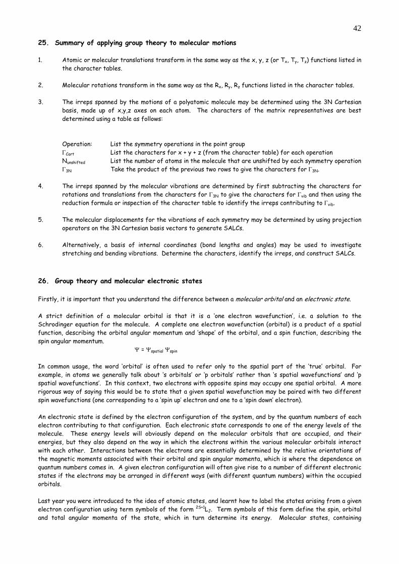
42

25. Summary of applying group theory to molecular motions 1. Atomic or molecular translations transform in the same way as the x, y, z (or Tx, Ty, Tz) functions listed in

the character tables.

2. Molecular rotations transform in the same way as the Rx, Ry, Rz functions listed in the character tables.

3. The irreps spanned by the motions of a polyatomic molecule may be determined using the 3N Cartesian basis, made up of x,y,z axes on each atom. The characters of the matrix representatives are best determined using a table as follows:

Operation: List the symmetry operations in the point group ΓCart List the characters for x + y + z (from the character table) for each operation Nunshifted List the number of atoms in the molecule that are unshifted by each symmetry operation

Γ3N Take the product of the previous two rows to give the characters for Γ3N. 4. The irreps spanned by the molecular vibrations are determined by first subtracting the characters for

rotations and translations from the characters for Γ3N to give the characters for Γvib and then using the reduction formula or inspection of the character table to identify the irreps contributing to Γvib.

5. The molecular displacements for the vibrations of each symmetry may be determined by using projection operators on the 3N Cartesian basis vectors to generate SALCs.

6. Alternatively, a basis of internal coordinates (bond lengths and angles) may be used to investigate

stretching and bending vibrations. Determine the characters, identify the irreps, and construct SALCs. 26. Group theory and molecular electronic states Firstly, it is important that you understand the difference between a molecular orbital and an electronic state. A strict definition of a molecular orbital is that it is a ‘one electron wavefunction’, i.e. a solution to the Schrodinger equation for the molecule. A complete one electron wavefunction (orbital) is a product of a spatial function, describing the orbital angular momentum and ‘shape’ of the orbital, and a spin function, describing the spin angular momentum. Ψ = Ψspatial Ψspin In common usage, the word ‘orbital’ is often used to refer only to the spatial part of the ‘true’ orbital. For example, in atoms we generally talk about ‘s orbitals’ or ‘p orbitals’ rather than ‘s spatial wavefunctions’ and ‘p spatial wavefunctions’. In this context, two electrons with opposite spins may occupy one spatial orbital. A more rigorous way of saying this would be to state that a given spatial wavefunction may be paired with two different spin wavefunctions (one corresponding to a ‘spin up’ electron and one to a ‘spin down’ electron). An electronic state is defined by the electron configuration of the system, and by the quantum numbers of each electron contributing to that configuration. Each electronic state corresponds to one of the energy levels of the molecule. These energy levels will obviously depend on the molecular orbitals that are occupied, and their energies, but they also depend on the way in which the electrons within the various molecular orbitals interact with each other. Interactions between the electrons are essentially determined by the relative orientations of the magnetic moments associated with their orbital and spin angular momenta, which is where the dependence on quantum numbers comes in. A given electron configuration will often give rise to a number of different electronic states if the electrons may be arranged in different ways (with different quantum numbers) within the occupied orbitals. Last year you were introduced to the idea of atomic states, and learnt how to label the states arising from a given electron configuration using term symbols of the form 2S+1LJ. Term symbols of this form define the spin, orbital and total angular momenta of the state, which in turn determine its energy. Molecular states, containing

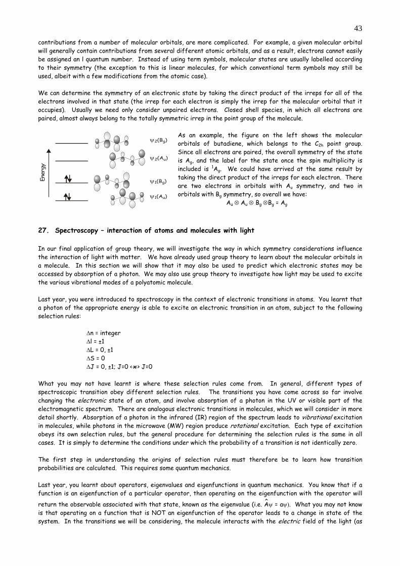
43

contributions from a number of molecular orbitals, are more complicated. For example, a given molecular orbital will generally contain contributions from several different atomic orbitals, and as a result, electrons cannot easily be assigned an l quantum number. Instead of using term symbols, molecular states are usually labelled according to their symmetry (the exception to this is linear molecules, for which conventional term symbols may still be used, albeit with a few modifications from the atomic case). We can determine the symmetry of an electronic state by taking the direct product of the irreps for all of the electrons involved in that state (the irrep for each electron is simply the irrep for the molecular orbital that it occupies). Usually we need only consider unpaired electrons. Closed shell species, in which all electrons are paired, almost always belong to the totally symmetric irrep in the point group of the molecule.

As an example, the figure on the left shows the molecular orbitals of butadiene, which belongs to the C2h point group. Since all electrons are paired, the overall symmetry of the state is Ag, and the label for the state once the spin multiplicity is included is 1Ag. We could have arrived at the same result by taking the direct product of the irreps for each electron. There are two electrons in orbitals with Au symmetry, and two in orbitals with Bg symmetry, so overall we have: Au ⊗ Au ⊗ Bg ⊗Bg = Ag

27. Spectroscopy – interaction of atoms and molecules with light In our final application of group theory, we will investigate the way in which symmetry considerations influence the interaction of light with matter. We have already used group theory to learn about the molecular orbitals in a molecule. In this section we will show that it may also be used to predict which electronic states may be accessed by absorption of a photon. We may also use group theory to investigate how light may be used to excite the various vibrational modes of a polyatomic molecule. Last year, you were introduced to spectroscopy in the context of electronic transitions in atoms. You learnt that a photon of the appropriate energy is able to excite an electronic transition in an atom, subject to the following selection rules: Δn = integer Δl = ±1 ΔL = 0, ±1 ΔS = 0 ΔJ = 0, ±1; J=0 <-->x J=0 What you may not have learnt is where these selection rules come from. In general, different types of spectroscopic transition obey different selection rules. The transitions you have come across so far involve changing the electronic state of an atom, and involve absorption of a photon in the UV or visible part of the electromagnetic spectrum. There are analogous electronic transitions in molecules, which we will consider in more detail shortly. Absorption of a photon in the infrared (IR) region of the spectrum leads to vibrational excitation in molecules, while photons in the microwave (MW) region produce rotational excitation. Each type of excitation obeys its own selection rules, but the general procedure for determining the selection rules is the same in all cases. It is simply to determine the conditions under which the probability of a transition is not identically zero. The first step in understanding the origins of selection rules must therefore be to learn how transition probabilities are calculated. This requires some quantum mechanics. Last year, you learnt about operators, eigenvalues and eigenfunctions in quantum mechanics. You know that if a function is an eigenfunction of a particular operator, then operating on the eigenfunction with the operator will

return the observable associated with that state, known as the eigenvalue (i.e. Aψ = aψ). What you may not know is that operating on a function that is NOT an eigenfunction of the operator leads to a change in state of the system. In the transitions we will be considering, the molecule interacts with the electric field of the light (as

Ener

gy

ψ2 g(B )

ψ2 u(A )

ψ1 u(A )

ψ1 g(B )

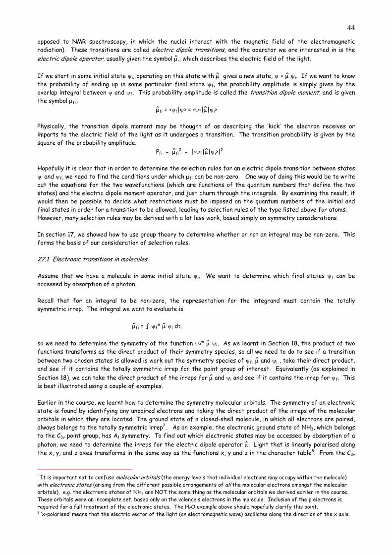
44

opposed to NMR spectroscopy, in which the nuclei interact with the magnetic field of the electromagnetic radiation). These transitions are called electric dipole transitions, and the operator we are interested in is the electric dipole operator, usually given the symbol μ., which describes the electric field of the light. If we start in some initial state ψi, operating on this state with μ gives a new state, ψ = μ ψi. If we want to know the probability of ending up in some particular final state ψf, the probability amplitude is simply given by the overlap integral between ψ and ψf. This probability amplitude is called the transition dipole moment, and is given the symbol μfi..

μfi = <ψf|ψ> = <ψf|μ|ψi> Physically, the transition dipole moment may be thought of as describing the ‘kick’ the electron receives or imparts to the electric field of the light as it undergoes a transition. The transition probability is given by the square of the probability amplitude.

Pfi = μfi2 = |<ψf|μ|ψi>|2

Hopefully it is clear that in order to determine the selection rules for an electric dipole transition between states ψi and ψf, we need to find the conditions under which μfi can be non-zero. One way of doing this would be to write out the equations for the two wavefunctions (which are functions of the quantum numbers that define the two states) and the electric dipole moment operator, and just churn through the integrals. By examining the result, it would then be possible to decide what restrictions must be imposed on the quantum numbers of the initial and final states in order for a transition to be allowed, leading to selection rules of the type listed above for atoms. However, many selection rules may be derived with a lot less work, based simply on symmetry considerations. In section 17, we showed how to use group theory to determine whether or not an integral may be non-zero. This forms the basis of our consideration of selection rules. 27.1 Electronic transitions in molecules Assume that we have a molecule in some initial state ψi. We want to determine which final states ψf can be accessed by absorption of a photon. Recall that for an integral to be non-zero, the representation for the integrand must contain the totally symmetric irrep. The integral we want to evaluate is μfi = ∫ ψf* μ ψi dτ, so we need to determine the symmetry of the function ψf* μ ψi. As we learnt in Section 18, the product of two functions transforms as the direct product of their symmetry species, so all we need to do to see if a transition between two chosen states is allowed is work out the symmetry species of ψf, μ and ψi , take their direct product, and see if it contains the totally symmetric irrep for the point group of interest. Equivalently (as explained in Section 18), we can take the direct product of the irreps for μ and ψi and see if it contains the irrep for ψf. This is best illustrated using a couple of examples. Earlier in the course, we learnt how to determine the symmetry molecular orbitals. The symmetry of an electronic state is found by identifying any unpaired electrons and taking the direct product of the irreps of the molecular orbitals in which they are located. The ground state of a closed-shell molecule, in which all electrons are paired, always belongs to the totally symmetric irrep7. As an example, the electronic ground state of NH3, which belongs to the C3v point group, has A1 symmetry. To find out which electronic states may be accessed by absorption of a photon, we need to determine the irreps for the electric dipole operator μ. Light that is linearly polarised along the x, y, and z axes transforms in the same way as the functions x, y and z in the character table8. From the C3v

7 It is important not to confuse molecular orbitals (the energy levels that individual electrons may occupy within the molecule) with electronic states (arising from the different possible arrangements of all the molecular electrons amongst the molecular orbitals). e.g. the electronic states of NH3 are NOT the same thing as the molecular orbitals we derived earlier in the course. These orbitals were an incomplete set, based only on the valence s electrons in the molecule. Inclusion of the p electrons is required for a full treatment of the electronic states. The H2O example above should hopefully clarify this point. 8 ‘x-polarised’ means that the electric vector of the light (an electromagnetic wave) oscillates along the direction of the x axis.

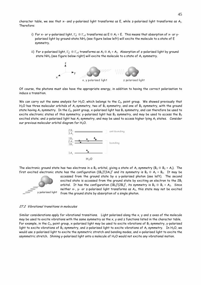
45

character table, we see that x- and y-polarised light transforms as E, while z-polarised light transforms as A1. Therefore:

i) For x- or y-polarised light, Γμ ⊗ Γψ1 transforms as E ⊗ A1 = E. This means that absorption of x- or y- polarised light by ground-state NH3 (see figure below left) will excite the molecule to a state of E symmetry.

ii) For z-polarised light, Γμ ⊗ Γψ1 transforms as A1 ⊗ A1 = A1. Absorption of z-polarised light by ground state NH3 (see figure below right) will excite the molecule to a state of A1 symmetry.

x

y

z

x, y polarised ligh t z po larised light Of course, the photons must also have the appropriate energy, in addition to having the correct polarisation to induce a transition. We can carry out the same analysis for H2O, which belongs to the C2v point group. We showed previously that H2O has three molecular orbitals of A1 symmetry, two of B1 symmetry, and one of B2 symmetry, with the ground state having A1 symmetry. In the C2v point group, x-polarised light has B1 symmetry, and can therefore be used to excite electronic states of this symmetry; y-polarised light has B2 symmetry, and may be used to access the B2 excited state; and z-polarised light has A1 symmetry, and may be used to access higher lying A1 states. Consider our previous molecular orbital diagram for H2O.

b onding

a nt ib onding 2B13A1

1A1

1B22A11B1

H O2

The electronic ground state has two electrons in a B2 orbital, giving a state of A1 symmetry (B2 ⊗ B2 = A1). The first excited electronic state has the configuration (1B2)1(3A1)1 and its symmetry is B2 ⊗ A1 = B2. It may be

accessed from the ground state by a y-polarised photon (see left). The second excited state is accessed from the ground state by exciting an electron to the 2B1 orbital. It has the configuration (1B2)1(2B1)1, its symmetry is B2 ⊗ B1 = A2. Since neither x-, y- or z-polarised light transforms as A2, this state may not be excited from the ground state by absorption of a single photon.

27.2 Vibrational transitions in molecules Similar considerations apply for vibrational transitions. Light polarised along the x, y and z axes of the molecule may be used to excite vibrations with the same symmetry as the x, y and z functions listed in the character table. For example, in the C2v point group, x-polarised light may be used to excite vibrations of B1 symmetry, y-polarised light to excite vibrations of B2 symmetry, and z-polarised light to excite vibrations of A1 symmetry. In H2O, we would use z-polarised light to excite the symmetric stretch and bending modes, and x-polarised light to excite the asymmetric stretch. Shining y-polarised light onto a molecule of H2O would not excite any vibrational motion.

y polarised light

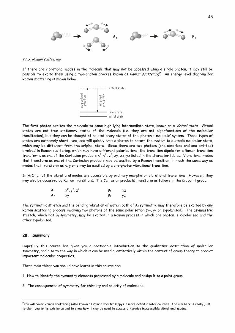
46

B1A 1

27.3 Raman scattering If there are vibrational modes in the molecule that may not be accessed using a single photon, it may still be possible to excite them using a two-photon process known as Raman scattering9. An energy level diagram for Raman scattering is shown below.

in iti al st at ef ina l st at e

vi rtu a l s ta te

abso

rbed

ph

oton

emitted

photon

The first photon excites the molecule to some high-lying intermediate state, known as a virtual state. Virtual states are not true stationary states of the molecule (i.e. they are not eigenfunctions of the molecular Hamiltonian), but they can be thought of as stationary states of the ‘photon + molecule’ system. These types of states are extremely short lived, and will quickly emit a photon to return the system to a stable molecular state, which may be different from the original state. Since there are two photons (one absorbed and one emitted) involved in Raman scattering, which may have different polarisations, the transition dipole for a Raman transition transforms as one of the Cartesian products x2, y2, z2, xy, xz, yz listed in the character tables. Vibrational modes that transform as one of the Cartesian products may be excited by a Raman transition, in much the same way as modes that transform as x, y or z may be excited by a one-photon vibrational transition. In H2O, all of the vibrational modes are accessible by ordinary one-photon vibrational transitions. However, they may also be accessed by Raman transitions. The Cartesian products transform as follows in the C2v point group. A1 x2, y2, z2 B1 xz A2 xy B2 yz The symmetric stretch and the bending vibration of water, both of A1 symmetry, may therefore be excited by any Raman scattering process involving two photons of the same polarisation (x-, y- or z-polarised). The asymmetric stretch, which has B1 symmetry, may be excited in a Raman process in which one photon is x-polarised and the other z-polarised. 28. Summary Hopefully this course has given you a reasonable introduction to the qualitative description of molecular symmetry, and also to the way in which it can be used quantitatively within the context of group theory to predict important molecular properties. These main things you should have learnt in this course are: 1. How to identify the symmetry elements possessed by a molecule and assign it to a point group. 2. The consequences of symmetry for chirality and polarity of molecules.

9You will cover Raman scattering (also known as Raman spectroscopy) in more detail in later courses. The aim here is really just to alert you to its existence and to show how it may be used to access otherwise inaccessible vibrational modes.

47

3. The effect of applying two or more symmetry operations consecutively (group multiplication) 4. How to construct a matrix representation of a group, starting from a suitable set of basis functions. 5. How to determine the irreducible representations (irreps) spanned by a basis set, and construct symmetry adapted linear combinations (SALCs) of the original basis functions that transform as the irreps of the group. 6. How to construct molecular orbitals by taking linear combinations of SALCs of the same symmetry species. (7. How to set up and solve the secular equations for the molecule in order to find the molecular energy levels and orbital coefficients – “Extra for experts”, though you will cover this in later courses) 8. How to determine the symmetries of the various modes of motion (translational, rotational and vibrational) of a polyatomic molecule, and the symmetries of individual vibrational modes. 9. How to determine the atomic displacements in a given vibrational mode by constructing SALCs in the 3N Cartesian basis. 10. How to determine atomic displacements in stretching and bending vibrations using internal coordinates. 11. The consequences of symmetry for the selection rules governing excitation to different electronic and vibrational states.

48

29. Appendix A – a few proofs for the mathematically inclined 1. Proof that the character of a matrix representative is invariant under a similarity transform. A property of traces of matrix products is that they are invariant under cyclic permutation of the matrices. i.e. tr[ABC] = tr[BCA] = tr[CAB]. For the character of a matrix representative of a symmetry operation g, we therefore have:

χ(g) = tr[Γ(g)] = tr[CΓ ’(g)C-1] = tr[Γ ’(g)C-1C] = tr[Γ’(g)] = χ’(g)

The trace of the similarity transformed representative is therefore the same as the trace of the original representative. 2. Proof that the characters of two symmetry operations in the same class are identical The formal requirement for two symmetry operations g and g’ to be in the same class is that there must be some symmetry operation f of the group such that g’=f-1gf (the elements g and g’ are then said to be conjugate). If we consider the characters of g and g’ we find: χ(g’) = tr[Γ(g’)] = tr[Γ -1(f) Γ(g) Γ(f)] = tr[Γ(g) Γ(f) Γ -1(f)] = tr[Γ(g)] = χ(g) The characters of g and g’ are identical. 3. Proof of the variation theorem. The variation theorem states that given a system with a Hamiltonian H, then if φ is any normalised, well-behaved function that satisfies the boundary conditions of the Hamiltonian, then

<φ|H|φ> ≥ Eo (1)

where E0 is the true value of the lowest energy eigenvalue of H. This principle allows us to calculate an upper bound for the ground state energy by finding the trial wavefunction φ for which the integral is minimised (hence the name; trial wavefunctions are varied until the optimum solution is found). Let us first verify that the variational principle is indeed correct. We first define an integral

I = <φ|-E0|φ> = <φ|H|φ> - <φ|E0|φ> = <φ|H|φ> - E0 <φ|φ> = <φ|H|φ> - E0 (since φ is normalised) If we can prove that I ≥ 0 then we have proved the variation theorem. Let ψi and Ei be the true eigenfunctions and eigenvalues of H, so H ψi = Ei ψi. Since the eigenfunctions ψi form a complete basis set for the space spanned by H, we can expand any wavefunction φ in terms of the ψi (so long as φ satisfies the same boundary conditions as ψi). φ =Σk akψk

Substituting this function into our integral I gives I = < Σk akψk | H-E0 | Σj ajψj >

49

= < Σk akψk | Σj (H-E0) ajψj > If we now use Hψ = Eψ, we obtain I = < Σk akψk | Σj aj (Ej-E0) ψj > = Σk Σj ak*aj (Ej-E0) < ψk | ψj > = Σk Σj ak*aj (Ej-E0) δjk We now perform the sum over j, losing all terms except the j=k term, to give I = Σk ak*ak (Ek-E0) = Σk |ak|2 (Ek-E0) Since E0 is the lowest eigenvalue, Ek-E0 must be positive, as must |ak|2. This means that all terms in the sum are non-negative and I ≥ 0 as required. For wavefunctions that are not normalised, the variational integral becomes:

<φ|H|φ >

<φ|φ > ≥ E0

4. Derivation of the secular equations – the general case of the linear variation method In the study of molecules, the variation principle is often used to determine the coefficients in a linear variation function, a linear combination of n linearly independent functions f1, f2, ..., fn (often atomic orbitals) that satisfy the boundary conditions of the problem. i.e. φ = Σi cifi. The coefficients ci are parameters to be determined by minimising the variational integral. In this case, we have: <φ|H|φ > = < Σi cifi |H| Σj cjfj >

= Σi Σj ci*cj <fi|H|fj > = Σi Σj ci*cj Hij where Hij is the Hamiltonian matrix element.

<φ|φ > = < Σi cifi | Σj cjfj > = Σi Σj ci*cj <fi|fj > = Σi Σj ci*cj Sij where Sij is the overlap matrix element.

The variational energy is therefore

E = Σi Σj ci*cj Hij

Σi Σj ci*cj Sij

which rearranges to give

E Σi Σj ci*cj Sij = Σi Σj ci*cj Hij

We want to minimise the energy with respect to the linear coeffients ci, requiring that ∂E ∂ci

= 0 for all i.

Differentiating both sides of the above expression gives,

∂E ∂ck

Σi Σj ci*cj Sij + E Σi Σj ⎣⎡

⎦⎤∂ci*

∂ckcj +

∂cj

∂ckci* Sij = Σi Σj ⎣

⎡⎦⎤∂ci*

∂ckcj +

∂cj

∂ckci* Hij

Since ∂ci*∂ck

= δik and Sij = Sji, Hij=Hji, we have

50

∂E

∂ck Σi Σj ci*cj Sij + 2E Σi Sik = 2 Σi ciHik

When ∂E∂ck

= 0, this gives

Σi ci(Hi k-ESik) = 0 for all k SECULAR EQUATIONS

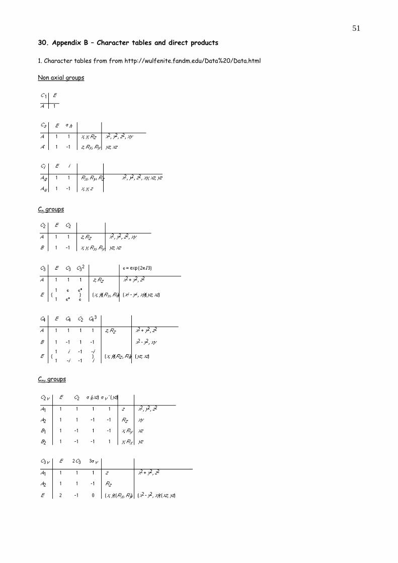
51

30. Appendix B – Character tables and direct products 1. Character tables from from http://wulfenite.fandm.edu/Data%20/Data.html Non axial groups

Cn groups

Cnv groups

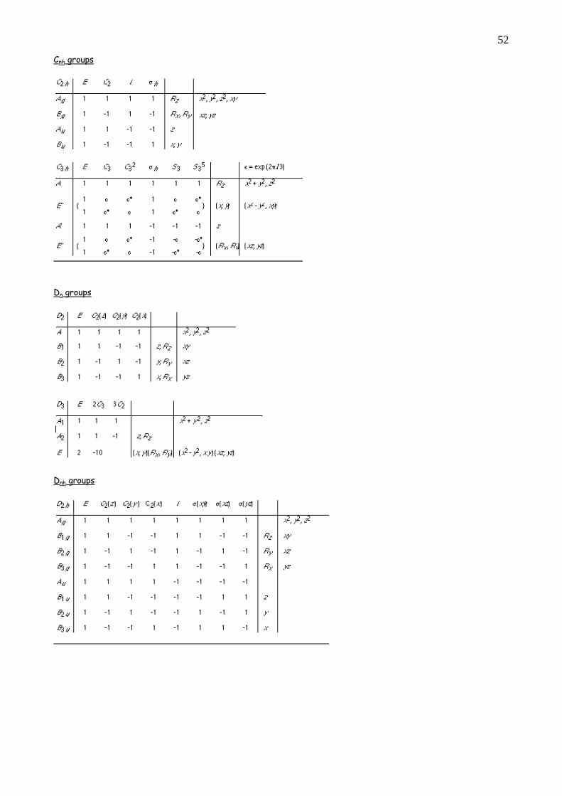
52

Cnh groups

Dn groups

Dnh groups

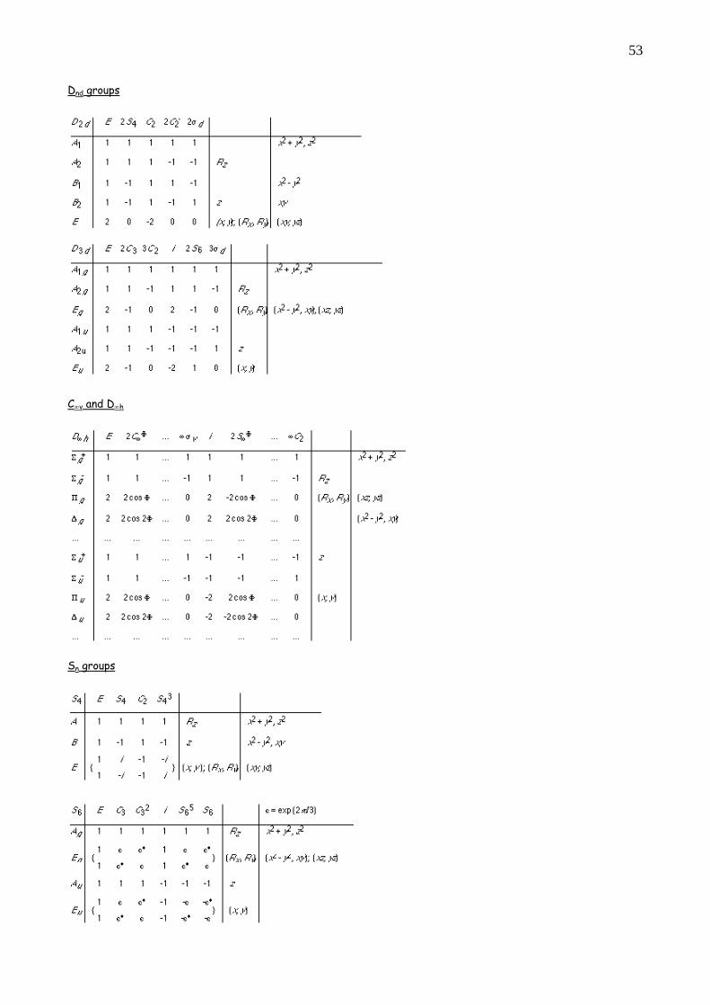
53

Dnd groups

C∞v and D∞h

Sn groups

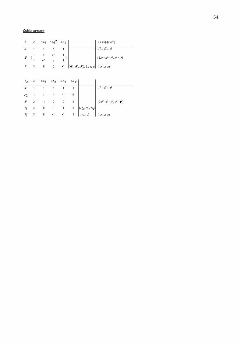
54

Cubic groups

55

2. Direct product tables For the point groups O and Td (and Oh) A1 A2 E T1 T2 A1 A1 A2 E T1 T2 A2 A1 E T2 T1 E A1+A2+E T1+T2 T1+T2 T1 A1+E+T1+T2 A2+E+T1+T2 T2 A1+E+T1+T2 For the point groups D4, C4v, D2d (and D4h = D4 ⊕ Ci) A1 A2 B2 B2 E A1 A1 A2 B1 B2 E A2 A1 B2 B1 E B1 A1 A2 E B2 A1 E E A1+A2+B1+B2

For the point groups D3 and C3v A1 A2 E A1 A1 A2 E A2 A1 E E A1+A2+E For the point groups D6, C6v and D3h* A1 A2 B1 B2 E1 E2 A1 A1 A2 B1 B2 E1 E2 A2 A1 B2 B1 E1 E2 B1 A1 A2 E2 E1 B2 A1 E2 E1 E| A1+A2+E2 B1+B2+E1 E2 A1+A2+E2 *in D3h make the following changes in the above table In table In D3h A1 A1’ A2 A2’ B1 A1’’ B2 A2’’ E1 E’’ E2 E’

56

PROBLEM SHEET – MOLECULAR SYMMETRY, GROUP THEORY, & APPLICATIONS Q1. Draw sketches to illustrate the following symmetry elements: a) a vertical mirror plane and a C2 axis in O3 (ozone) b) a horizontal mirror plane in CO2 c) an S4 axis in methane d) all of the symmetry elements in CH3F (point group C3v) e) all of the symmetry elements in ethene (point group D2h) Q2. Determine the symmetry elements possessed by an s orbital, a p orbital, a dz

2 orbital, and a dxy orbital Q3. Which of the following molecules has i) a centre of inversion and ii) an S4 axis? a) CO2 b) C2H2 c) BF3 d) SO4

2- Q4. Identify the symmetry elements in the following molecules, and assign each one to a point group (use the

flow diagram in the lecture notes if you find this helpful). a) NH2Cl b) SiF4 c) H-C≡N d) SiFClBrI e) NO2 f) H2O2 Q5. a) What are the symmetry elements that prevent a molecule from being polar? Which of the molecules in Q4 are polar?

b) What are the symmetry elements that exclude chirality? Which (if any) of the molecules in Q4 may be chiral?

Q6. What are the symmetry operations in the point group C2v? Identify a molecule that belongs to the group.

By examining the effect of sequential application of the various symmetry operations in the group, construct the group multiplication table.

Q7. a) How can group theory be used to determine whether an integral can be non-zero? b) Use group theory to determine whether the following integrals are non-zero (use the tables of direct products provided in the lecture handout). i) the overlap integral between a px orbital and a pz orbital in the point group C2v ii) the overlap integral between a px orbital and a dxz orbital in the point group C3v iii) the overlap integral between a py orbital and a dz

2 orbital in the point group Td iv) the overlap integral between a pz orbital and a dz

2 orbital in the point group D2h

c) Which of the following electronic transitions are symmetry allowed? i) a transition from a state ofA1 symmetry to a state of E1 symmetry excited by z-polarised light in a molecule belonging to the point group C5v.

57

ii) a transition from a state of A1g symmetry to a state of A2u symmetry excited by z-polarised light in a molecule belonging to the point group D∞h. iii) a transition from a state of B2 symmetry to a state of B1 symmetry excited by y-polarised light in a molecule belonging to the point group C2v.

Q8. Consider the hydronium ion H3O+. This ion has a pyramidal structure with one HOH bond angle smaller

than the other two, and belongs to the point group CS.

a) Using a basis set consisting of a 1s orbital on each H atom and 2s, 2px, 2py and 2pz orbitals on the O atom (i.e. (sO,px,py,pz,s1,s2,s3)), construct a matrix representation.

b) What are the characters of each of the matrix representatives?

c) What are the irreps spanned by the basis?

d) Use the basis to construct a set of SALCs.

e) Write down the general form of the molecular orbitals of H3O+.

Q9. Consider the chlorobenzene molecule C6H5Cl. a) What is the molecular point group?

b) Use a basis made up of a p orbital on each carbon atom (pointing perpendicular to the benzene ring) to construct the π molecular orbitals using the following steps:

i) determine the character of each symmetry operation ii) determine the irreps spanned by the basis iii) construct a set of SALCs and take linear combinations to form the molecular orbitals of each symmetry species.

Q10. a) Use the 3N Cartesian basis and the character table for the C3v point group to determine the symmetries of the vibrational modes of NH3. b) Use a basis of internal coordinates to determine the symmetries of the stretching vibrations only. Hence classify each of the vibrational modes found in a) as a bending or a stretching vibration.

c) Construct SALCs using the internal coordinate basis to determine the atomic displacements associated with each stretching mode. Draw each mode, and label it as a symmetric or asymmetric stretching vibration. It is quite complicated to use the 3N Cartesian basis to construct SALCs in this case (though you are welcome to try). What do you think the A1 bending vibration looks like? Identify the A1 and E bending vibrations as symmetric or antisymmetric. d) Which vibrational modes could be excited by i) a one-photon process ii) a two-photon process? What are the polarisations of the photons involved in each case?