Molecular symmetry effects on non-adiabatic coupling terms and quantum reaction dynamics via

conical intersections

Jörn ManzFreie Universität Berlin

Acknowledgments- Freie Universität Berlin group - Al Quds University group

M. Leibscher, PhD. Prof. O. DeebProf. D. Haase S. Al-Jabour

- Hebrew University Jerusalem groupProf. M. BaerProf. S. ZilbergDr. X. Xu

Quantum Chemistry

Molecular Symmetry *

Quantum Dynamics

* NOT molecular point groupBunker, P. R.;Jensen, P., Molecular Symmetry and Spectroscopy; NRC Research Press, Ottawa 1998.S. Al-Jabour, M. Baer, O. Deeb, M. Leibscher, J. Manz, X. Xu, S. Zilberg; J. Phy. Chem. A, in press

Outline:

Molecular point group versus molecular symmetry groupMS- adapted coordinatesLocating the CIs using Longuet-Higgins loopsDetermination of the irreducible representations (IREPs) of NACTsApplying molecular Symmetry rule on C5H4NH NACTCharges and IREPs of conical intersectionsSeam of conical intersectionsEffects of NACTs on Quantum Reaction Dynamics

Molecular point group versus molecular symmetry group

Molecular symmetry group: global (all feasible inversion and permutation which commute with the Hamiltonian)

o Molecular point group: only for local structures (minima, transition states, conical intersection)

cis“syn”

trans“anti”

Example: Cyclopenta-2,4-dienimine

Character table

coordinatesσ’vσvC2EC2v

z1111A1

-1-111A2

x-11-11B1

y1-1-11B2

MS adapted coordinates

(12)*E*(12)EC2v(M)

?1111A1

?“q”

-1-111A2

?-11-11B1

?1-1-11B2

- Symmetry projection operators and symmetry adapted coordinates

Molecular point group Molecular symmetry group

Example:

xxCExP VVB =−+−= )(

41 '

21 σσ qqEEqP A =−−+= ))12()12((

41 **2

“x has B1 symmetry” “q has A2 MS symmetry”

1st. Goal: construct MS- adapted coordinates

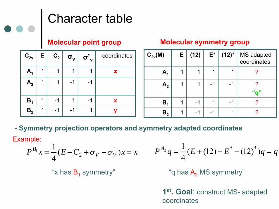
In general: 3N-6 symmetry adapted coordinates, these describe feasible motions of large and small amplitudes

Model: small amplitudes: frozenlarge amplitude: moving

Example:torsion angle (φ) describing cis-trans isomerization reaction.

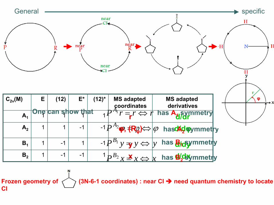
specific

One can show that

xxxP

yyyP

P

rrrP

B

B

A

A

⇔=

⇔=

⇔=

⇔=

2

1

2

1

ϕϕϕ

MS adapted derivatives

MS adapted coordinates

d/drrφ, (Rφ)

yx

1111A1

d/dφ-1-111A2

d/dy-11-11B1

d/dx1-1-11B2

(12)*E*(12)EC2v(M)

has A2 symmetry

has A1 symmetry

has B1 symmetry

has B2 symmetry

φ

Frozen geometry of (3N-6-1 coordinates) : near CI need quantum chemistry to locate CI

General

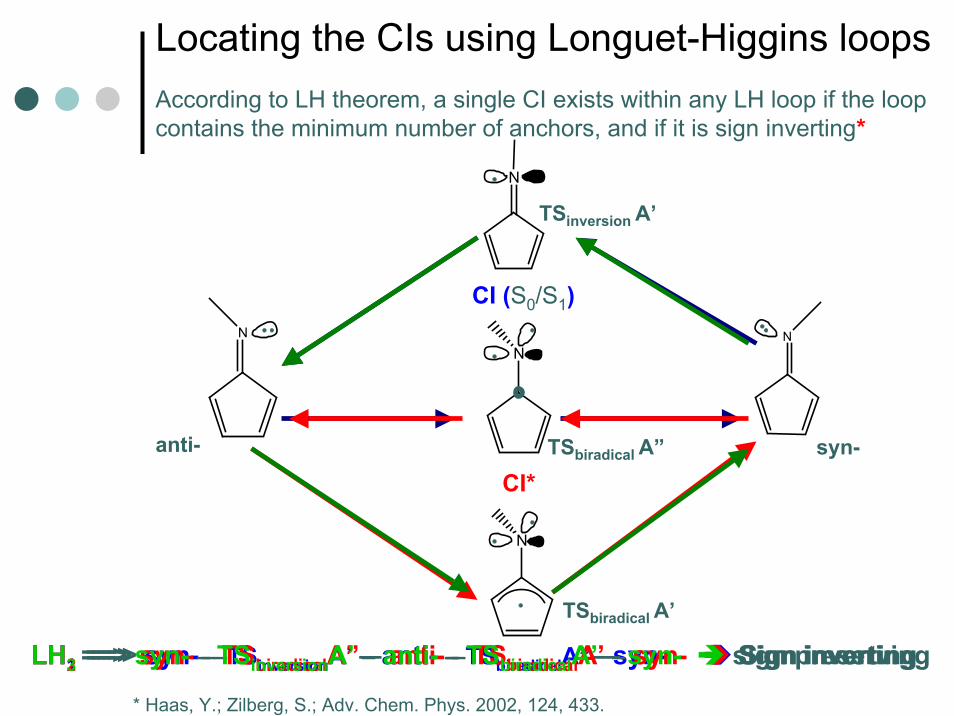
Locating the CIs using Longuet-Higgins loops

NN

N

N

N

syn-anti- TSbiradical A”

TSbiradical A’

TSinversion A’

LH1 ==> syn- –TSinversionA’ – anti- – TSbiradicalA”– syn- Sign inverting

CI (S0/S1)

CI*

LH2 ==> syn- – TSbiradicalA” – anti- – TSbiradicalA’ – syn- Sign invertingLH3 ==> syn- – TSinversionA’ – anti- – TSbiradicalA’ – syn- sign preserving

According to LH theorem, a single CI exists within any LH loop if the loop contains the minimum number of anchors, and if it is sign inverting*

* Haas, Y.; Zilberg, S.; Adv. Chem. Phys. 2002, 124, 433.

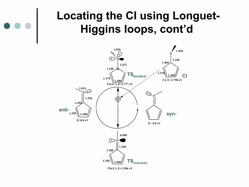
Locating the CI using Longuet-Higgins loops, cont’d

N

N

N

N

N

E=0.0 eVE= 0.0 eV

TS(A'), E=1.586 eV

TS(A''), E=2.777 eVCI, E=2.798 eV

1.2961.490

1.350 1.490

1.014

1.2601.500

1.500

1.4321.440

1.3701.480

1.3981.460

1.3701.490

CI

0.980

1.020 1.020

1.350

TSbiradical

TSinversion

CI

syn-anti-

E

0

*

* Planar geometry close to S0/S1CI (and minima) is frozen

N

Fragment has local C2v symmetry

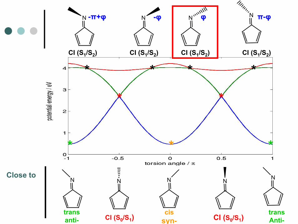
N NN NN

N NN N

transanti- CI (S0/S1)

cissyn- CI (S0/S1)

transAnti-

CI (S1/S2)CI (S1/S2)CI (S1/S2)CI (S1/S2)

*

* * * *

π-φ-φ φ-π+φ

*

**

*

Close to

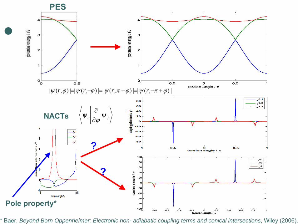
|),(||),(||),(||),(| ϕπψϕπψϕψϕψ +−=−=−= rrrr

NACTs ji ψψϕ∂∂

?

?

Pole property*

* Baer, Beyond Born Oppenheimer: Electronic non- adiabatic coupling terms and conical intersections, Wiley (2006).

PES

Determination of the irreducible representations (IREPs) of NACTs

Step 1: sign and nodal patterns

Step 2: theorem of NACTs in C2v(M)

ji

ji

ji

rji

rji

r

rr

r

,

211

,

)||( IREP

A A A

)()()( IREP

)()()( IREP

ϕ

ϕ

ϕ

τ

ψϕ

ψ

ϕψψ

ϕτ

=

∂∂

=

⋅⋅Γ⋅⋅Γ=∂∂

Γ⋅∂∂

Γ⋅∂∂

=

∂∂

Γ⋅∂∂

Γ⋅Example:

In general: )()( IREP IREP ji,,

lklji

k ∂∂

Γ⋅∂∂

Γ⋅= ττ

Character table Four possibilities

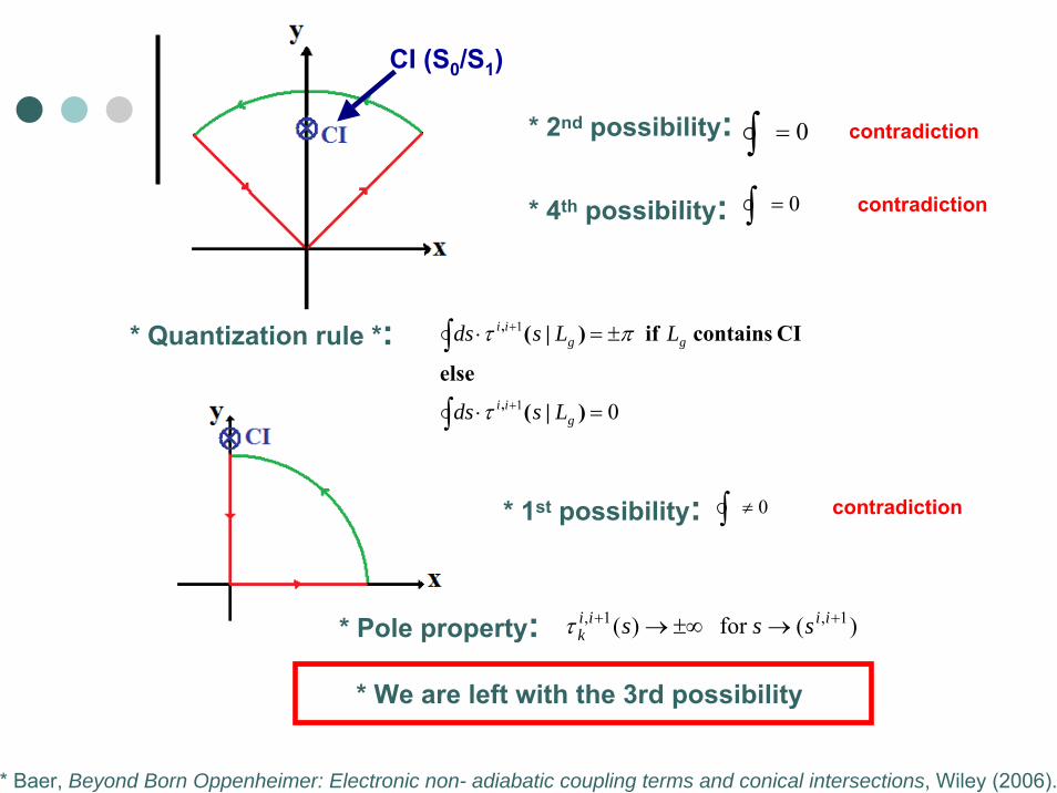
CI (S0/S1)

* 2nd possibility:

0=∫

0=∫

0≠∫

contradiction

* 4th possibility: contradiction

* 1st possibility: contradiction

* We are left with the 3rd possibility

01

1

=⋅

±=⋅

∫

∫

+

+

)|(

else

CI contains if )|(

,

,

gii

ggii

Lsds

LLsds

τ

πτ* Quantization rule *:

)(for )( 1,1, ++ →±∞→ iiiik sssτ* Pole property:

* Baer, Beyond Born Oppenheimer: Electronic non- adiabatic coupling terms and conical intersections, Wiley (2006).

Character table Four possibilities

ϕϕπϕπ

ϕττ ϕϕ

−+−−⇒ ,,at einterchang also they

),/(S CInear at einterchang and NACTs 1,,

22010 S

12,01,0 BIREP same thehave and =⇒ ϕϕ ττ

2nd theorem for NACTs

Example

In general

loop gerade if Aelse

loop ungerade if )( IREP.... )( IREP)( IREP

1

z,0k

1,2k

0,1k

=

Γ=⋅⋅⋅

k

τττ

2,

222221120

210

1,

1

,,,

A)( IREP

A A A A

|| IREP|| IREP|| IREP

B )( IREP B

)( IREP)( IREP)( IREP

=⇒

=Γ⋅⋅Γ⋅Γ⋅⋅Γ⋅Γ⋅⋅Γ=

∂∂

⋅∂∂

⋅∂∂

=

⋅⋅=

⋅⋅

21

0

021

21

022110

ϕ

ϕ

ϕϕϕ

τ

ψϕ

ψψϕ

ψψϕ

ψ

τ

τττ0

12

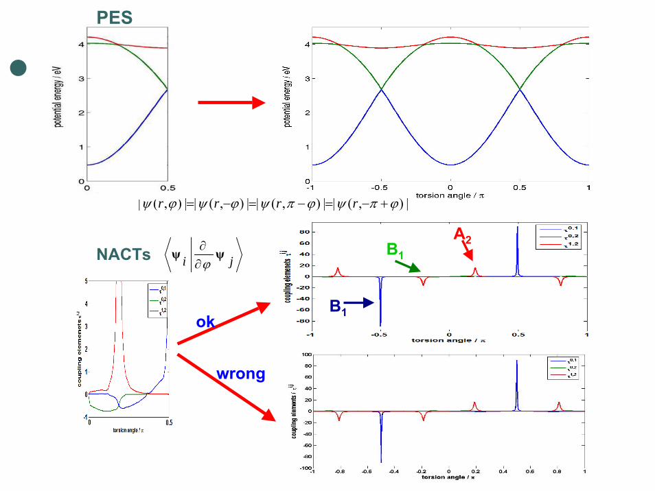
|),(||),(||),(||),(| ϕπψϕπψϕψϕψ +−=−=−= rrrr

NACTs ji ψψϕ∂∂

wrong

ok

A2B1

B1

PES

Charges and IREPs of conical intersections

Example: CI (S0/S1)11,0

1 +=e

11,02 −=e

Example: CI (S1/S2)

ππτ ⋅=±=+∫ igii eLsds )|( if , 1

Then charge ei of CI is ±1

Arbitrary choice

Due to IREP of NACTsCI (S0/S1) has IREP B1CI (S1/S2) has IREP A2

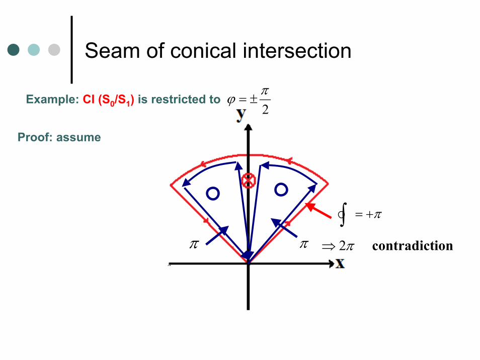
Seam of conical intersection

2πϕ ±=

ioncontradict π2⇒π

Example: CI (S0/S1) is restricted to

Proof: assume

π π

π+=∫

Seam of CIsCI (S1/S2) for all φ CI (S0/S1) only for φ = π /2

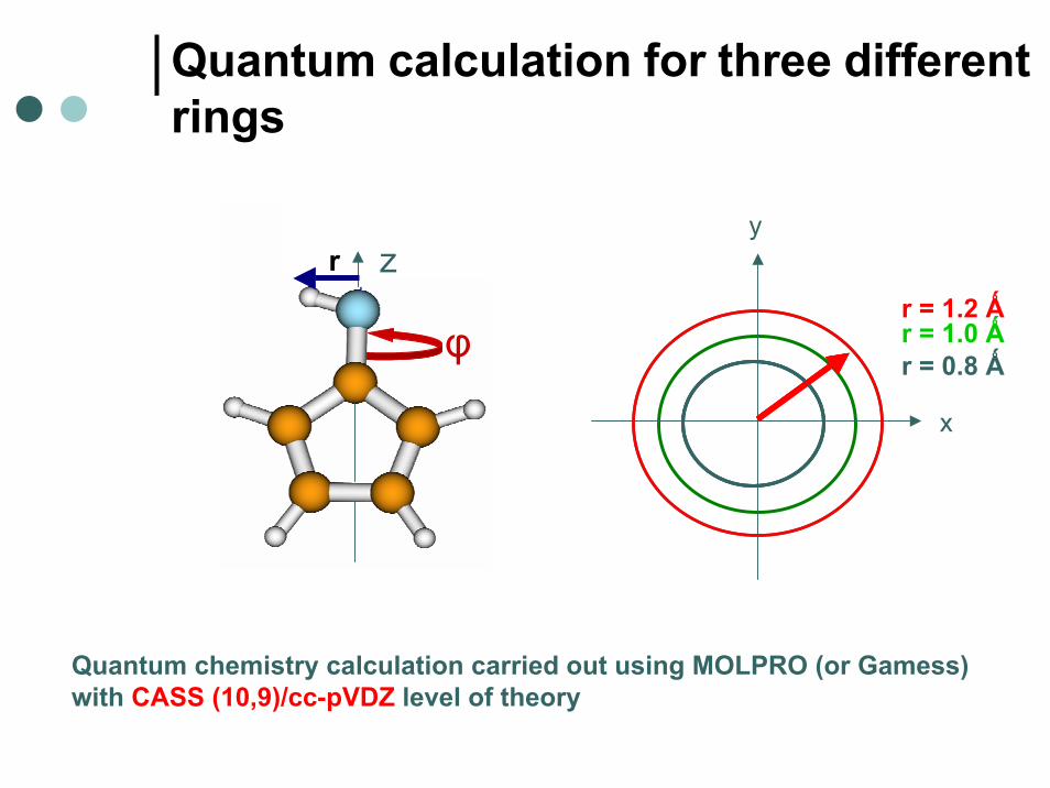
Quantum calculation for three different rings

x

yz

φ

rr = 1.2 Ǻr = 1.0 Ǻr = 0.8 Ǻ

Quantum chemistry calculation carried out using MOLPRO (or Gamess) with CASS (10,9)/cc-pVDZ level of theory

Small ring

middle ring

Large ring

Adiabatic potentials and NACTs of C5H4NH

V i/e

V

Effect of NACTs on Quantum Reaction Dynamics

adadad irI

i ψ V ) τ()(

ψ +−∂∂

−= 2

21

ϕh&h

diadiadia Ii ψ ) W

2(ψ 2

22

+∂∂

−=ϕ

h&h

1A

),( A))~,(τ~( exp ) A(

0 A τ A

0

00

=

⋅=⇒

=+∂∂

∫ 0ϕϕϕϕ

ϕϕ

ϕ ϕ rrdr,

*

Adiabatic :

)2,(W)0,(W),(A ),(V ),(A),(W †

πϕϕϕϕ

rrrrrr addia

==

diabatic :

quantization :

* Baer, M.; Chem. Phys. Lett. 1975, 35,112.

•Baer, M., Beyond Born Oppenheimer: Electronic non- adiabatic coupling •terms and conical intersections, Wiley (2006).

),(ψ),(A),(ψ ϕϕϕ rrr addia =

Adiabatic to diabatic potential

W00W11W22

V0V1V2

A00A11A22

torsion angle

torsion angle

torsion angle

adia

batic

pot

entia

l

diab

atic

pote

ntia

l

Dia

gona

l ele

men

t of A

Diabatic potentials are not MS symmetric !W is only a mathematical tool, no physical meaning

Photoinduced Dynamics

Initial state: ground torsional state S0 of syn-C5H4NHShort laser pulse excites wavepacket S0 S2 (Franck-Condon excitation)Wavepacket propagation in diabatic represntation with split-operator-method*

“syn” “anti”

* Schmidt, Lorenz, WavePacket 4.5 (2008).

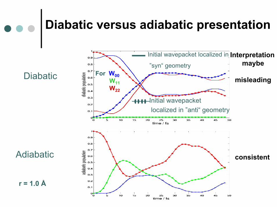
Diabatic versus adiabatic presentation

Initial wavepacket localized in

”syn“ geometry

Initial wavepacketlocalized in ”anti“ geometry

For W00W11W22

Diabatic

Adiabatic

r = 1.0 Å

Interpretation maybe

misleading

consistent

Does IREP of NACTs effects reaction dynamics?!

Small ring, two cases r= 0.8 Å

Case B

hypothetical

Case AMS

Reaction dynamics propagation result

Case A

Case B

* Radiationless decay depends on IREP of NACTs

Conclusions:

IREP of NACTs and CIs can be assigned according to MS group.New result beyond traditional quantum chemistryPhotoinduced dynamics, e.g. radiationlessdecay depends on IREP of NACTsNew result beyond traditional quantum reaction dynamics

Berlin group

Peace is in the waves at sea.Peace must begin with you and me

To tell the worldno more violence

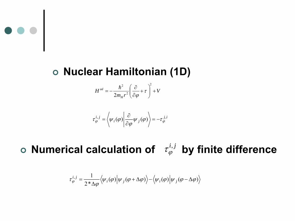
Nuclear Hamiltonian (1D) V

rmH

H

ad +⎟⎟⎠

⎞⎜⎜⎝

⎛+

∂∂

−=2

2

2

2τ

ϕh

ijji

ji ,, )()( ϕϕ τϕψϕ

ϕψτ −=∂∂

=

Numerical calculation of by finite differenceji,ϕτ

)()()()(*21, ϕϕψϕψϕϕψϕψϕ

τϕ Δ−−Δ+Δ

= jijiji