Molecular Structure-nonlinear Optical Property ...

University of Central Florida University of Central Florida

STARS STARS

Electronic Theses and Dissertations, 2004-2019

2006

Molecular Structure-nonlinear Optical Property Relationships For Molecular Structure-nonlinear Optical Property Relationships For

A Series Of Polymethine And Squaraine Molecules A Series Of Polymethine And Squaraine Molecules

Jie Fu University of Central Florida

Part of the Electromagnetics and Photonics Commons, and the Optics Commons

Find similar works at: https://stars.library.ucf.edu/etd

University of Central Florida Libraries http://library.ucf.edu

This Doctoral Dissertation (Open Access) is brought to you for free and open access by STARS. It has been accepted

for inclusion in Electronic Theses and Dissertations, 2004-2019 by an authorized administrator of STARS. For more

information, please contact [email protected].

STARS Citation STARS Citation Fu, Jie, "Molecular Structure-nonlinear Optical Property Relationships For A Series Of Polymethine And Squaraine Molecules" (2006). Electronic Theses and Dissertations, 2004-2019. 1016. https://stars.library.ucf.edu/etd/1016

https://stars.library.ucf.edu/



https://stars.library.ucf.edu/etd

http://network.bepress.com/hgg/discipline/271?utm_source=stars.library.ucf.edu%2Fetd%2F1016&utm_medium=PDF&utm_campaign=PDFCoverPages

http://network.bepress.com/hgg/discipline/204?utm_source=stars.library.ucf.edu%2Fetd%2F1016&utm_medium=PDF&utm_campaign=PDFCoverPages

https://stars.library.ucf.edu/etd

http://library.ucf.edu/

mailto:[email protected]

https://stars.library.ucf.edu/etd/1016?utm_source=stars.library.ucf.edu%2Fetd%2F1016&utm_medium=PDF&utm_campaign=PDFCoverPages



MOLECULAR STRUCTURE – NONLINEAR OPTICAL PROPERTY RELATIONSHIPS FOR A SERIES OF POLYMETHINE AND

SQUARAINE MOLECULES

by

JIE FU B.S. Tsinghua University, 1997 M.S. Tsinghua University, 2000

M.S. University of Central Florida, 2002

A dissertation submitted in partial fulfillment of the requirements for the degree of Doctor of Philosophy

in the College of Optics and Photonics: CREOL & FPCE at the University of Central Florida

Orlando, Florida

Fall Term 2006

Major Professors: Dr. Eric W. Van Stryland and Dr. David J. Hagan

© 2006 Jie Fu

ii

ABSTRACT

This dissertation reports on the investigation of the relationships between molecular

structure and two-photon absorption (2PA) properties for a series of polymethine and squaraine

molecules. Current and emerging applications exploiting the quadratic dependence upon laser

intensity, such as two-photon fluorescence imaging, three-dimensional microfabrication, optical

data storage and optical limiting, have motivated researchers to find novel materials exhibiting

strong 2PA. Organic materials are promising candidates because their linear and nonlinear

optical properties can be optimized for applications by changing their structures through

molecular engineering. Polymethine and squaraine dyes are particularly interesting because they

are fluorescent and showing large 2PA.

We used three independent nonlinear spectroscopic techniques (Z-scan, two-photon

fluorescence and white-light continuum pump-probe spectroscopy) to obtain the 2PA spectra

revealing 2PA bands, and we confirm the experimental data by comparing the results from the

different methods mentioned.

By systematically altering the structure of polyemthines and squaraines, we studied the

effects of molecular symmetry, strength of donor terminal groups, conjugation length of the

chromophore chain, polarity of solvents, and the effects of placing bridge molecules inside the

chromophore chain on the 2PA properties. We also compared polymethine, squaraine,

croconium and tetraon dyes with the same terminal groups to study the effects of the different

additions inserted within the chromophore chain on their optical properties. Near IR absorbing

squaraine dyes were experimentally observed to show extremely large 2PA cross sections (≈

30000GM). A simplified three-level model was used to fit the measured 2PA spectra and

iii

detailed quantum chemical calculations revealed the reasons for the squaraine to exhibit strong

2PA. In addition, two-photon excitation fluorescence anisotropy spectra were measured through

multiple 2PA transitions. A theoretical model based on four-levels with two intermediate states

was derived and used for analysis of the experimental data.

iv

This dissertation is dedicated to my parents and my wife Xiang Wu, who have given me

unending patience, support and love throughout these years.

v

ACKNOWLEDGMENTS

I would truly like to thank my advisors, Dr. David J. Hagan and Dr. Eric W. Van Stryland,

for providing me this great opportunity and environment to complete my graduate research work

in CREOL. I really appreciate their every effort to provide me the guidance whenever I needed

throughout these years because both of them also take great responsibility on the CREOL and

OSA at same time, so have very tight schedule.

I also deeply grateful for the opportunity to work with Dr. Olga A. Przhonska from the

Institute of Physics, National Academy of Sciences of Ukraine. Without her great patience and

detailed discussions, this dissertation would not have been possible. Not only I learned a lot from

her about chemistry of organic molecule, but also her incredible passions and dedications on the

science put herself a valuable example to anyone working with her.

The whole of the work presented in this dissertation was result of a truly broad

collaborative effort. I want to sincerely thank Dr. Lazaro A. Padilha for his extensive

experimental work on Z-scan measurements. He is a great friend as well. I also want to give

special thanks to former student Dr. Joel M. Hales for his help and encouragement. He taught me

much of what I know about femto-second lab and scientific research in my earlier years here. I

also appreciate people from Institute of Organic Chemistry of National Academy of Sciences

from Ukraine, Dr. Seth Marder’s group at School of Chemistry and Biochemistry from Georgia

Institute of Technology and Dr. Kevin Belfield’s group for their great efforts on synthesizing the

organic molecules studied in this dissertation.

I would like to thank the graduate students and post-docs I have worked with in the

nonlinear optics group over the years. Dr. Scott Webster is a great group leader, researcher and

vi

friend. I also appreciate all the help from Dr. Rich Lepkowicz, Ion Cohanoschi, Peter Olszak,

Claudiu Cirloganu and Mihaela Balu.

Finally I want to thank all of my friends and acquaintances I’ve made here while in

CREOL. Dr. Changching Tsai, Dr. S.T. Wu’s group, Dr. Guifang Li’s group, Peter Olszak,

Weiyao Zhou, you all made this one of best times of my life. Thank you to everyone.

vii

TABLE OF CONTENTS

LIST OF FIGURES ....................................................................................................................... xi

LIST OF TABLES....................................................................................................................... xix

LIST OF NOMENCLATURE..................................................................................................... xxi

CHAPTER 1 INTRODUCTION .................................................................................................... 1

1.1 Background and motivation.................................................................................................. 1

1.2 Dissertation statement........................................................................................................... 7

1.3 Dissertation outline ............................................................................................................... 7

CHAPTER 2 NONLINEAR OPTICS AND TWO-PHOTON ABSORPTION THEORY............ 9

2.1 Nonlinear optics/macroscopic polarization theory ............................................................... 9

2.2 Two-photon absorption and perturbation theory ................................................................ 15

2.2.1 Two-photon absorption................................................................................................ 15

2.2.2 Calculation for third-order nonlinear susceptibility..................................................... 19

CHAPTER 3 LINEAR AND NONLINEAR SPECTROSCOPY METHODS............................ 32

3.1 Linear spectroscopic techniques ......................................................................................... 32

3.2 Nonlinear spectroscopy....................................................................................................... 34

3.2.1 Femtosecond 1KHz laser system................................................................................. 34

3.2.2 Z-scan........................................................................................................................... 35

3.2.3 Two-Photon Fluorescence (2PF) Spectroscopy........................................................... 37

3.2.4 White-Light Continuum Pump-Probe Spectroscopy ................................................... 43

3.2.5 Pump-probe experiments to study ESA and 2PA processes........................................ 46

CHAPTER 4 STRUCTURE-PROPERTY RELATIONSHIP OF POLYMETHINE DYES....... 53

4.1 Cyanines.............................................................................................................................. 53

viii

4.2 Polymethine dyes ................................................................................................................ 54

4.3 Symmetry............................................................................................................................ 57

4.4 Terminal groups .................................................................................................................. 60

4.5 Conjugation length.............................................................................................................. 64

4.6 Polarity of solvents ............................................................................................................. 69

4.7 Effect of bridge ................................................................................................................... 75

CHAPTER 5 STRUCTURE-PROPERTY OF SQUARAINE, CROCONIUM AND TETRAON

....................................................................................................................................................... 78

5.1 Squaraine dyes .................................................................................................................... 78

5.2 Comparison between polymethines and squaraines ........................................................... 79

5.3 Quantum-chemical calculations and analysis ..................................................................... 85

5.3.1 Methodology of quantum-chemical calculations......................................................... 85

5.3.2 Unsubstituted polymethine chain................................................................................. 88

5.3.3 Polymethines................................................................................................................ 91

5.3.4 Squaraines .................................................................................................................... 96

5.4 Squaraine molecules showing large 2PA cross sections................................................... 100

5.5 Croconium and Tetraon .................................................................................................... 110

5.5.1 Squaraine Vs Croconium ........................................................................................... 110

5.5.2 Squaraine Vs Tetraon................................................................................................. 112

5.6 Relations of one-photon anisotropy to 2PA spectra ......................................................... 115

5.6.1 One-photon excitation fluorescence anisotropy......................................................... 115

5.6.2 Polymethine dyes ....................................................................................................... 116

5.6.3 Squaraine dyes ........................................................................................................... 120

ix

CHAPTER 6 TWO-PHOTON EXCITATION FLUORESCENCE ANISOTROPY ................ 123

6.1 Introduction....................................................................................................................... 123

6.2 Experimental setup............................................................................................................ 124

6.3 Two-photon anisotropy: four-state and three-state model ................................................ 125

6.4. Symmetric molecules....................................................................................................... 128

6.4.1.Analysis: Three-state model ...................................................................................... 131

6.4.2. Analysis: Four-state model ....................................................................................... 132

6.4.3. Analysis: Symmetry breaking of symmetric molecules ........................................... 133

6.5. Asymmetric molecules..................................................................................................... 135

6.6 Why do we use the four-state model?............................................................................... 136

CHAPTER 7 CONCLUSIONS .................................................................................................. 140

7.1 Conclusions....................................................................................................................... 140

7.2 Future work....................................................................................................................... 143

APPENDIX A CGS AND SI UNIT ........................................................................................... 145

APPENDIX B EXPERIMENTAL DATA FOR MOLECULES FROM DR. OLGA V.

PRZHONSKA............................................................................................................................. 148

APPENDIX C EXPERIMENTAL DATA FOR MOLECULES FROM DR. SETH R.

MARDER’S GROUP ................................................................................................................. 155

APPENDIX D DERIVATIONS FOR TWO-PHOTON EXCITATION FLUORESCENCE

ANISOTROPY ........................................................................................................................... 178

LIST OF REFERENCES............................................................................................................ 184

x

LIST OF FIGURES

Figure 1.1 Diagram for electronic transitions for Excited State Absorption (ESA) and Two-

Photon Absorption (2PA) ............................................................................................. 2

Figure 1.2 Illustration showing a comparison of fluorescence due to 1PA (a) and 2PA (b) to

show the greater spatial resolution of two-photon excitation ....................................... 4

Figure 1.3 Photophysical process following 2PA (S0, S1 and S2 are singlet states, T1 is a triplet

state): 1) Internal Conversion to S1; 2) Intersystem crossing (ISC) to triplet state T1; 3)

radiative decay (fluorescence) from S1; 4) Excited state absorption (ESA)................. 4

Figure 1.4: (a) Molecular structure for ethane (b) illustration of covalent bands of ethane ........... 5

Figure 2.1 Three state model for Sum-Over-State (SOS) expression........................................... 24

Figure 3.1 Femto-second 1KHz laser system with tunable wavelength output............................ 35

Figure 3.2 (a) Z-scan experimental setup (b) typical open-aperture Z-scan experimental data

(square) with theoretical fitting (red line)................................................................... 36

Figure 3.3 Fluorescence following one-photon absorption (a) and two-photon absorption (b) ... 38

Figure 3.4 Experimental setup for two-photon fluorescence spectroscopy using femtosecond

laser pulses from the TOPAS...................................................................................... 39

Figure 3.5 Experimental setup for white-light continuum pump-probe nonlinear spectroscopy.

BS-Beam Splitter, λ/2-half waveplate, P-polarizer, RR-retroreflector....................... 44

Figure 3.6 (a) Linear absorption spectrum for TOR-I-103 in THF (b) The normalzied

transmission of probe as a function of the time delay between pump and probe pulses

for TOR-I-103 with pump 1020nm (2uJ, 3uJ and 4.5uJ) and probe 1064nm. Solid

lines are for eye-guide................................................................................................. 47

xi

Figure 3.7 (a) Linear absorption spectrum of Sjz-3-16 in THF; (b) The normalzied transmission

of probe 650nm as a function of the time delay between pump and probe pulses for

Sjz-3-16 with pump 600nm (3uJ, 6uJ and 9uJ) and probe 650nm. ESA signals are

indicated by ∆1, ∆2 and ∆3 for three pump energies respectively; (c) Plot of logarithm

of ESA signal (∆) as a function of logarithm of pump energy ................................... 49

Figure 3.8 (a) Linear absorption spectrum of LB-II-80 in THF; (b) The normalzied transmission


LB-II-80 with pump 600nm. ESA signals are indicated by ∆3, ∆4 and ∆5 for pump

energies 3uJ, 6uJ and 9uJ respectively. ESA signals for pump enegies 0.5uJ and 1uJ

are equal to ∆1 = 0.002, ∆2 = 0.005 respectively (not shown in the graph); (c) Plot of

logarithm of ESA signal (∆) as a function of logarithm of pump energy................... 50

Figure 3.9 (a) Linear absorption spectrum of LB-II-80 in THF; (b) The normalzied transmission


LB-II-80 with pump 690nm. ESA signals are indicated by ∆1, ∆2, ∆3 and ∆4 for pump

energies 3uJ, 7uJ, 10uJ and 13uJ respectively. (c) Plot of logarithm of ESA signal (∆)

as a function of logarithm of pump energy................................................................. 52

Figure 4.1 (a) General molecular structure of PD, R1 and R2 are terminal groups; (b) π-electron

distribution in polymethine chromophore................................................................... 54

Figure 4.2 Molecular structures of Polymethine Dyes (PDs) ....................................................... 55

Figure 4.3 (a) Molecular structures (b) Degenerate 2PA spectra for PD2350 (red), PD2665 (black)

and PD2755 (blue). Dashed line is the theoretical fitting based on Eq. (2.55), and the

linear absorption spectra (solid line) are shown for reference.................................... 58

xii

Figure 4.4 (a) Molecular structures (b) Degenerate 2PA spectra for PD25 (red), Styryl_1 (black).

The dashed line is for theoretical fitting based on Eq. (2.55), and linear absorption

spectra (solid line) are shown for reference................................................................ 59

Figure 4.5 (a) Molecular structures; (b) Degenerate 2PA spectra for PD 2630, PD 2350 and PD

2646. The dashed line is for theoretical fitting based on Eq. (2.55), and linear

absorption spectra (solid line) are shown for reference. ............................................. 61

Figure 4.6 (a) Molecular Structure (b) Degenerate 2PA spectra for PD 200 and PD 2761. The

dashed line is for theoretical fitting based on Eq. (2.55), and linear absorption spectra

(solid line) are shown for reference ............................................................................ 63

Figure 4.7 (a) molecular structures; (b) degenerate 2PA spectra for PDAF, PD2350, PD3428 and

PD824,. The dashed line is for theoretical fitting based on Eq. (2.55), and linear

absorption spectra (solid line) are shown for reference. ............................................. 66

Figure 4.8 (a) molecular structures; (b) degenerate 2PA spectra for PD25, PD2646 and PD2501.

The dashed line is for theoretical fitting based on Eq. (2.55), and linear absorption

spectra (solid line) are shown for reference................................................................ 67

Figure 4.9 Molecular structures for the study of the solvent effect on the weak 2PA band......... 70

Figure 4.10 Linear absorption and fluorescence spectra for PD 2646 and PD 2755 in different

solvents ....................................................................................................................... 71

Figure 4.11 2PA spectra for PD 2646 in different solvents: methanol (black), ethanol (red) and

1,2-Dichlorobenzene (blue). Dashed line is a guide for the eye. Solid lines are linear

absorption spectra in different solvents for comparison. ............................................ 73

xiii

Figure 4.12 2PA spectra for PD 2755 in different solvents: ethanol (blue) and 1,2-

Dichlorobenzene (red). Dashed line is for a guide for the eye. Solid lines are linear

absorption spectra in different solvents for comparison. ............................................ 74

Figure 4.13 (a) molecular structures; (b) degenerate 2PA spectra for PD200, PD2646, dashed line

is for theoretical fitting based on Eq. (2.55), and linear absorption spectra (solid line)

are shown for reference............................................................................................... 75

Figure 4.14 (a) molecular structures; (b) degenerate 2PA spectra for PD3428, PD2093, dashed

line is for theoretical fitting based on Eq. (2.55), and linear absorption spectra (solid

line) are shown for reference. ..................................................................................... 76

Figure 5.1 Squaraine dyes (SDs): (a) electron acceptor C4O2 fragment at the center of the chain,

R1 and R2 are terminal groups; (b) SDs synthesized in Institute of Organic Chemistry,

National Academy of Sciences, Ukraine .................................................................... 79

Figure 5.2 (a) Molecular structure of PD2350 and SD2577; (b) Linear absorption and

fluorescence spectra in ethanol; (c) 2PA spectra in ethanol (dotted, dashed line for

theoretical fitting) and linear absorption spectra (solid lines) shown as extinction

coefficient ................................................................................................................... 81

Figure 5.3 (a) Molecular structure of PD2630 and SD2243; (b) Linear absorption and

fluorescence spectra; (c) 2PA spectra (doted, dashed line for theoretical fitting) and

linear absorption spectra shown as extinction coefficient. PD 2630 in ethanol and SD

2243 in CH2CL2 .......................................................................................................... 82

Figure 5.4 Scheme of the electronic transitions for the unsubstituted chain, PD 2350 and SD

2577. Dashed lines indicate one-photon allowed transitions; solid lines indicate

xiv

allowed two-photon transitions; bold solid lines indicate experimentally observed

two-photon transitions. ............................................................................................... 88

Figure 5.5 Electron density distribution in the molecular orbitals for the unsubstituted

polymethine chain and indolium terminal groups. ..................................................... 90

Figure 5.6 Scheme of the energy levels for molecular orbitals of the unsubstituted polymethine

chain, indolium terminal groups and PD 2350. H identifies Highest Occupied

Molecular Orbital (HOMO) and L identifies Lowest Unoccupied Molecular Orbital

(LUMO). Dashed arrow lines indicate experimentally observed one-photon

transitions and solid arrow line indicatesw the experimentally observed two-photon

transition. .................................................................................................................... 91

Figure 5.7 Electron density distribution in the molecular orbitals for PD 2350........................... 92

Figure 5.8 Scheme of the energy levels for molecular orbitals of PD 2646, PD 2350 and PD

2630. H identifies the Highest Occupied Molecular Orbital (HOMO) and L identifies

the Lowest Unoccupied Molecular Orbital (LUMO). Dashed arrow lines indicate

experimentally observed one-photon transitions and solid arrow lines indicate

experimentally observed two-photon transitions. ....................................................... 95

Figure 5.9 Electron density distribution in the molecular orbitals for SD 2577........................... 97

Figure 5.10 Scheme of the energy levels for molecular orbitals of PD 2350 and SD 2577. H

identifies the Highest Occupied Molecular Orbital (HOMO) and L identifies the

Lowest Unoccupied Molecular Orbital (LUMO). Dashed arrow lines indicate

experimentally observed one-photon transitions and solid arrow lines indicate

experimentally observed two-photon transitions. ....................................................... 98

xv

Figure 5.11 Molecular structures of squaraine dyes synthesized by Seth Marder’s group at the

Georgia Institute of Technology ............................................................................... 101

Figure 5.12 2PA spectra for squaraine dyes synthesized by Seth Marder’s group at Georgia

Institute of Technology. 2PA cross-section δ is plotted versus the wavelength for 2PA

state (equivalent to sum of two excitation photons’ energies, for D-2PA, two photons

have same energies, for ND-2PA, pump and probe photons have different energies).

The pump wavelength of WLC pump-probe measurements for ND-2PA is shown in

the graph.................................................................................................................... 105

Figure 5.13 Two centrosymmetric conformers of TOR-I-103 considered in quantum chemical

calculations ............................................................................................................... 106

Figure 5.14 Molecular structure for (a) Squaraine TOR-I-110 (b) Croconium TOR-I-95......... 111

Figure 5.15 2PA spectra for squaraine TOR-I-110 and croconium TOR-I-95. Linear spectra also

are plotted for comparison. ....................................................................................... 112

Figure 5.16 Molecular structure for (a) Squaraine dye SD 2243 and (b) Tetraon dye TOD 2765.

................................................................................................................................... 113

Figure 5.17 2PA spectra for squaraine SD 2243 in CH2CL2 and tetraon TOD 2765 in Ethnaol.

Linear spectra also are plotted for comparison. ........................................................ 114

Figure 5.18 Experiment setup for one-photon and two-photon excitation fluorescence anisotropy

measurement ............................................................................................................. 115

Figure 5.19 Molecular structures for polymethine dyes: PD 2350, PD 2646 and PD 2630....... 117

Figure 5.20 One-photon excitation fluorescence anisotropy and 2PA spectra for three PDs with

different terminal groups. Linear spectra also are plotted for comparison. .............. 118

Figure 5.21 Molecular structures for squaraine dyes (a) SD 2577 (b) SC-V-21c ...................... 120

xvi

Figure 5.22 One-photon excitation fluorescence anisotropy and 2PA spectra for two SDs: (a) SD

2577 (b) SC-V-21c. There are two curves for one-photon anisotropy spectra: (1)

measured by the visible detector, PMT R928b (2) measured by the near IR PMT.

Linear spectra are also plotted for comparison. ........................................................ 121

Figure 6.1 Four-state, two-intermediate level (S1 and Sn ), model for two-photon anisotropy, (a)

energy states S0, S1, Sf and Sn diagram; (b) transition dipole moments schematic

diagram ..................................................................................................................... 126

Figure 6.2 Three-state one-intermediate level (S1) model for two-photon anisotropy: (a) energy

states S0, S1, Sf diagram; (b) transition dipole moments schematic diagram............ 127

Figure 6.3 Molecular structures for polymethine dyes PD2350, PD3428, PD2665 and Styryl_1

................................................................................................................................... 129

Figure 6.4 Molecule structures of two fluorene derivatives for two-photon excitation

fluorescence anisotropy measurements..................................................................... 129

Figure 6.5 (1) linear absorption, (2) 2PA, (3) one-photon fluorescence anisotropy and (4) two-

photon fluorescence anisotropy spectra for symmetric molecules; (a) PD2350; (b)

PD3428; (c) Fluorene 2............................................................................................. 130

Figure 6.6 Two-photon anisotropy as a function of the angle γ with the three-state model at (1)

αem=0° ; (2) 5°; (3) 10°; and (4) 20°. ........................................................................ 131

Figure 6.7 (a) Two-photon anisotropy PAr2 , calculated in the four-state model, as a function of γ.

αem = 100; µ01 =13.5 D; µ12 = µ04 = µ42 = 1 D; β = 600; φ = 00 (or 1800); ∆E1 = 0.5 eV;

∆E2 = 2.5 eV. This curve coincides with curve 3 from Fig. 6.7 obtained from the

three-state model. (b) 3D picture of PAr2 , calculated in the four-state model, as a

function of β and φ for αem = 100; µ01 =13.5 D; µ12 = µ04 = µ42 = 1 D; γ = 1800...... 133

xvii

Figure 6.8 Schematic presentation of the orientation of the transition dipole moments for (a)

symmetrical and (b) asymmetrical forms of PD 2350. µ”02 and µ’

02 indicate a partial

charge transfer from each terminal group to the polymethine chromophore............ 135

Figure 6.9 Linear absorption (1), 2PA spectra (2), one-photon anisotropy (3) and two-photon

anisotropy (4) for asymmetric molecules: (a) PD2665; (b) Styryl 1; (c) Fluorene 1.

................................................................................................................................... 136

Figure 6.10 (a) Two-photon anisotropy PAr2 for 2PA to S2 state of PD2350, calculated in the four-

state model, as a function of γ. Curve 1: αem = 100; β = 600; φ = 00 (or 1800); ∆E1 =

0.5 eV; ∆E2 = 2.5 eV; µ01 =13.5 D; µ12 =1D; µ04 = µ42 = 1 D. Curve 2 and 3: αem =

100; β = 600; ∆E1 = 0.5 eV; ∆E2 = 2.5 eV; µ01 =13.5 D; µ12 = 1 D; µ04 = µ42 = 6 D; φ

= 00 (for curve 2) and φ = 1800 (for curve 3). (b) 3D plot of PAr2 , as functions of β, φ ,

with αem = 100; γ = 1800; ∆E1 = 0.5 eV; ∆E2 = 2.5 eV; µ01 =13.5 D; µ12 = 1 D; µ04 =

µ42 = 6 D ................................................................................................................... 137

Figure 6.11 Calculated wavelength dependence of PAr2 under 2PA to S1 state (1) and 2PA to S2

state (2) based on the four-state model. Molecular parameters for (1) are: αem = 100;

µ01 =13.5 D; ∆µ = 0.6; µ02 = 1.2 D; µ21 = 1 D; φ = 900; β = 320; γ = 550. Molecular

parameters for (2) are: αem = 100; µ01 =13.5 D; µ12 = 1 D; µ04 = µ42 = 1 D; φ = 1800;

β = 600; γ = 1630. ...................................................................................................... 139

xviii

LIST OF TABLES

Table 2.1 Second-order nonlinear optical processes related to second-order susceptibility χ(2) .. 14

Table 2.2 Third-order nonlinear optical processes related to third-order susceptibilityχ(3) ......... 15

Table 4.1 Linear optical properties of polymethine dyes in ethanol............................................. 56

Table 4.2 Parameters for PDs having the same conjugate length with benzoindolium (PD2630);

indolium (PD2350); thiazolium (PD2646) terminal groups......................................... 61

Table 4.3 Parameters for PD 200 and PD 2761 having the same conjugate length with different

terminal groups............................................................................................................. 63

Table 4.4 Parameters for PDs having indolium terminal groups with conjugation length from n=1

to n=4. Detuning energy ∆E is calculated for the 2PA peak at δ max2; Q. C. is from

the quantum chemical calculation

exp

................................................................................ 66

Table 4.5 Parameters for PDs having tiazolium terminal groups with conjugation length from

n=1 to n=3. Detuning energy ∆E is calculated for a 2PA peak at δ max2; Q. C. is

from the quantum chemical calculation

exp

....................................................................... 67

Table 4.6 Dielectric constant ε, refractive index n and polarity ∆f of the three solvents (methanol,

ethanol and 1,2-Dichlorobenzene) ............................................................................... 71

Table 5.1 Parameters for polymethine and squaraine with analogous structures: PD2350 and

SD2577 in ethanol ........................................................................................................ 80

Table 5.2 Parameters for polymethine and squaraine with analogous structures: PD2630 and

SD2243......................................................................................................................... 80

Table 5.3 Calculated parameters for the unsubstituted polymethine chain, PD 2350 and SD 2577

...................................................................................................................................... 87

xix

Table 5.4 Theoretical one and two-photon parameters for SC-V-21c and TOR-I-103 a............ 108

Table 5.5 Linear properties of squaraine TOR-I-110 and croconium TOR-I-95 in THF: linear

absorption peak λ max, extinction coefficient ε and ground state transition dipole

moment. µ

abs max

ge ................................................................................................................ 111

Table 5.6 Linear properties of squaraine SD 2243 in CH CL and tetraon TOD 2765 in ethanol:

linear absorption peak λ max, extinction coefficient ε and ground state transition

dipole moment µ

2 2

abs max

01 ...................................................................................................... 113

xx

LIST OF NOMENCLATURE

Acronym/Unit Description

2PA Two-Photon Absorption

2PF Two-Photon Fluorescence

CaF2 Calcium Fluoride

cm Centimeter (10-2 m)

D-2PA Degenerate Two-Photon Absorption

ESA Excited-State Absorption

eV Electron Volt unit of energy

fs Femtosecond (10-15 s)

GM Goppert-Mayer unit for the 2PA cross-section (1 x 10-50 cm4 sec

photon-1 molecule-1)

GVD Group-Velocity Dispersion

GVM Group-Velocity Mismatch

GW Gigawatt (109 W)

HOMO Highest Occupied Molecular Orbital

ISC Intersystem Crossing

kHz Kilohertz (103 Hz)

LUMO Lowest Unoccupied Molecular Orbital

µJ Microjoule (10-6 J)

µm Micrometer (10-6 m)

M Molarity unit of concentration (Moles/Liter)

xxi

mm Millimeter (10-3 m)

MW Megawatt (106 W)

ND-2PA Nondegenerate Two-Photon Absorption

nJ Nanojoule (10-9 J)

NLO Nonlinear Optical

nm Nanometer (10-9 m)

ns Nanosecond (10-15 s)

OD Optical Density

OKE Optical Kerr Effect

OPA Optical Parametric Amplifier

ps Picosecond (10-12s)

SOS Sum-Over-States

THF Tetrahydrofuran

WLC White Light Continuum

xxii

CHAPTER 1 INTRODUCTION

1.1 Background and motivation

In 1931, Maria Goppert-Mayer first theoretically predicted that an atom or a molecule

could absorb two photons simultaneously in a single quantized event [1]. The first experimental

evidence for two-photon absorption (2PA) waited 30 years until the laser was invented, and then

Kaiser and Garret demonstrated two-photon excitation in a CaF2:Eu3+ crystal [2].

The process of two-photon absorption involves simultaneous absorption of two photons

from an initial state to a higher excited state within a material, and the energy difference between

these two states is equal to the sum of the energies of the two photons. In the case of absorbing

two photons having the same frequency or photon energy, this type of 2PA is called Degenerate

2PA (D-2PA). In the case of absorbing two photons having different frequency or photon energy,

this type of 2PA is called Nondegenerate 2PA (ND-2PA).

The two-photon absorption process is different from excited state absorption (ESA). Both

of them involve two photons. The difference is shown in Fig.1.1. S0 is ground state, S1 is the first

excited state, and S2 is the second excited state.

1

S0

S1

S2

ESA

1

2

S0

S1

S2

ESA

1

2

S0

S1

S2

2PA

1

2

∆E

S0

S1

S2

2PA

1

2

S0

S1

S2

2PA

1

2

∆E

Figure 1.1 Diagram for electronic transitions for Excited State Absorption (ESA) and Two-Photon Absorption (2PA)

The following is a conceptual description of ESA and 2PA that provides some useful

intuition concerning the processes. Shown in Fig. 1.1, In the ESA process, photon 1 has

sufficient energy to excite a molecule from the ground state S0 to the first excited state S1.

Because the energy mismatch, ∆E, between photon 1 and state S1 is within the natural linewidth,

excited electrons can make real transitions and stay in state S1 for times of ~10-3 to 10-12 seconds.

Thus arrival of photon 2 within this time can complete the electronic transition to the final state

S2. This describes the ESA process, which is sometimes called resonance two-photon absorption.

In a 2PA process, the energy mismatch ∆E between photon 1 and the first excited state S1

is large compared to the natural linewidth and neither photon has sufficient energy to excite the

ground-state molecule to excited state S1 on its own. Thus, in order to complete the 2PA process

to S2, the second photon has to arrive within a time determined by the Uncertainty Principle [3].

The brief duration of this action (~10-15 seconds for 2PA in the visible) is the reason 2PA is

classified as an ‘instantaneous’ nonlinear process. This also describes why 2PA is observed only

for high intensity where the probability of finding 2 photons in the same time interval is large.

2PA is also called non-resonance two-photon absorption.

2

More accurately, the probability of 2PA depends quadratically on the irradiance of the

beam (2PA ∝ I2). This leads to several existing and potential applications and technologies,

including two-photon fluorescence microscopy [4], three-dimensional (3D) micro-fabrication [5]

and optical data storage [6].

Achieving 3D spatial resolution with 2PA (or spatial localization of 2PA) is illustrated in

Fig. 1.2. The solution is a fluorescent chromophore. In Fig.1.2 (a), light of wavelength λ1 is

focused into the solution. Because λ1 is within the linear absorption spectrum, the solution shows

large one-photon absorption (1PA) of the λ1 beam at regions close to the surface, and then emits

significant fluorescence from this region. In Fig.1.2 (b), the laser beam of wavelength λ2 (λ2 =

2λ1) is focused into the solution by the same focusing geometry. Because λ2 is not within the

linear absorption range, the green solution does not experience 1PA of λ2 at regions close to the

surface, and only experiences 2PA at region near the focal point where the intensity of the laser

beam is high. Fluorescence following 2PA is localized at the region of the focal point. Moreover,

the λ2 laser beam shows much less linear scattering loss (scattering loss ∝ ω4) compared with a

λ1 beam, so 2PA improves the penetration depth. This is important for biological imaging.

3

λ1λ2

(a) (b)

Fluorescence due to one-photon absorption

Fluorescence due to two-photon absorption

lens

solution

λ1λ1λ2λ2

(a) (b)

Fluorescence due to one-photon absorption

Fluorescence due to two-photon absorption

lens

solution

Figure 1.2 Illustration showing a comparison of fluorescence due to 1PA (a) and 2PA (b) to show the greater spatial resolution of two-photon excitation

In addition to the fluorescence that can follow the 2PA process, 2PA can also be followed

by intersystem crossing (ISC) and ESA as shown in Fig.1.3. Another important application of

2PA is optical power limiting [8-10] which takes advantage of these processes.

S0

S2

S1

1

2

3

4

4

4

T1

S0

S2

S1

1

2

3

4

4

4

T1

Figure 1.3 Photophysical process following 2PA (S0, S1 and S2 are singlet states, T1 is a triplet state): 1) Internal Conversion to S1; 2) Intersystem crossing (ISC) to triplet state T1; 3) radiative

decay (fluorescence) from S1; 4) Excited state absorption (ESA)

4

Organic materials are strong candidates for 2PA applications because their material

properties can be tailored through molecular engineering. In particular, electron delocalization in

molecules provides a strong polarizability to enhance a molecule’s 2PA.

In organic structures the delocalization of electrons, similar to the free electrons in a

semiconductor, is provided by π-bonding in a class of organic compounds called π-conjugated

molecules and polymers. These conjugated molecules involve alternate single and multiple

covalent bonds. A single covalent bond between two atoms (heavier than hydrogen) is formed by

the axial overlap of the hybridized atomic orbitals of two atoms and is called the σ bond (blue

bond in Fig.1.4). The additional bond involved in a double covalent bond between two atoms is

formed by the lateral overlap of the un-hybridized p type atomic orbitals (green bond in Fig.1.4).

This bond is called a π bond, and the electrons involved are called the π electrons. One example

for π bonds in ethane is illustrated in Fig.1.4 [11].

C CH

H

H

H

C

CH

H

H

Hσ band

π band

C

CH

H

H

Hσ band

π band

(a) (b)

Figure 1.4: (a) Molecular structure for ethane (b) illustration of covalent bands of ethane

5

A double covalent bond has one σ bond and one π bond, and a triple covalent bond has

one σ bond and two π bonds. π electrons are loosely bound electrons and are spread (delocalized)

over the entire conjugated molecular structure, hence behaving similar to free electrons in a

semiconductor.

Unfortunately, most known organic molecules have relatively small 2PA cross sections δ,

and criteria for the design of molecules with large δ have not been well developed. A significant

breakthrough came in 1998 [12] and opened the door for design strategies for molecules with

large 2PA cross sections. Researchers synthesized molecules with linear π-conjugation showing

large 2PA cross sections on the basis of the concept that symmetric charge (π electrons) transfers

from the ends of a conjugated system to the middle, or vice verse [12]. They also performed

quantum chemical calculations to confirm this charge redistribution with experimental results.

After that, various research groups [13-26] have shown molecular design strategies for

efficient 2PA by a systematic investigation of the conjugation length of the chromophores,

various symmetrical and asymmetrical combinations of electron-donor and electron-acceptor

terminal groups, and the addition of such groups in the middle of the chromophore to vary the

charge distribution. Even though there has been considerable progress in the studies of structure-

property relationships of organic molecules, much more remains to be discovered. We discuss

some of this in this dissertation but also use newly developed techniques (done at CREOL) to

significantly build the existing database to help elucidate structure/property relations in

collaboration with materials synthesizers and quantum chemists.

6

1.2 Dissertation statement

The purpose of this dissertation is to investigate several sets of organic molecules whose

structures have been systemically altered to determine how these structural changes will affect

their two-photon absorbing capabilities. Full linear spectroscopic characterization is performed

on these molecules to determine the strength, location and spectral contour of their absorption

and emission spectra. Several nonlinear spectroscopic techniques are employed to characterize

both the strength and location of the 2PA spectra. In addition, quantum chemical calculations are

used to determine state and transition dipole moments, as well as explaining and confirming

experimental results. We also measured two-photon excitation fluorescence anisotropy spectra

which for the first time covered several 2PA bands, giving us more insight into the 2PA process.

Molecular structure motif changes, such as symmetry, conjugation length, donor-acceptor

strength, effect of squaraine addition, croconium and tetraon are investigated. These results show

definitive correlations between chemical structures and the linear and nonlinear optical

properties of these molecules, and with molecules showing unprecedented 2PA cross sections.

All these experimental and theoretical studies improve our understanding of the way to optimize

molecular two-photon absorbing capabilities.

1.3 Dissertation outline

This work is structured according to the following: Chapter 1 introduces the concept of

two-photon absorption and provides the impetus for investigating this nonlinear behavior of

organic molecules. Chapter 2 describes this process in terms of light-matter interactions and

presents the perturbative Sum-Over-States (SOS) formulation for the third-order susceptibility,

7

χ(3). Chapter 3 addressed the linear and nonlinear spectroscopic techniques. Chapter 4

concentrates on the study of relationships between molecular structures and 2PA properties for

polymethine molecules. The linear spectroscopic data for these molecules are also presented.

Chapter 5 addresses the relationships between chemical structures and the 2PA properties of

squaraines. We also compared 2PA properties for polymethines, squaraines, croconium and

tetraon molecules having similar structures. Quantum chemical calculations help us understand

the differences and also provide us insight into the nature of the 2PA process. In Chapter 6, two-

photon excitation fluorescence anisotropy spectra of polymethines and squaraines are studied

both experimentally and theoretically. We derived a new equation for two-photon anisotropy

based on a two-intermediate-state, four-level model to reveal the orientation between different

transition dipole moments involved in the 2PA process. Finally, Chapter 7 concludes the

dissertation and suggests some future directions which might be taken.

8

CHAPTER 2 NONLINEAR OPTICS AND TWO-PHOTON ABSORPTION THEORY

2.1 Nonlinear optics/macroscopic polarization theory

All derivations and formulas in this chapter are based on the definition of the electric

field and polarization shown below:

( titi ee ωω ∗− += 00 EEE21 ) (2.1)

( titi ee ωω ∗− += 00 PPP21 ) (2.2)

Nonlinear optics studies the phenomena that the response of a material system to an

applied optical/electric field depends upon the strength of the optical field in a nonlinear manner,

or in the other words, optical properties of a material system are changed in the presence of an

intense optical field.

Responses of materials to intense optical fields depend on the frequency of the optical

wave and the irradiance (i.e. for pulsed sources, the pulse energy, pulse duration, and beam

spatial distribution): and on the materials; 1) displacement of electrons; 2) displacement of atoms

(molecular vibrations); 3) molecular orientation in liquid and gas phase; 4) electrostriction

(acousto-optics); 5) molecular orientation in solid (liquid crystal); 6) saturated absorption; 7)

thermal effect. Here two-photon absorption (2PA) is one of nonlinear optical processes related to

the displacement of electrons in the presence of an intense optical field.

Now we consider details of this interaction between materials and an externally applied

optical electric field, Eex. The materials consist of a distribution of charged particles, namely

9

positively charged nuclei and negatively charged electrons. In general, the electron is

“elastically” coupled to the nucleus (by “classical” picture). An externally applied oscillating

optical field Eex will interact with electrons in the way that electrons are “displaced” by the

electric field in the vicinity, called the local electric filed Eloc. This local field is due to the

externally applied optical field Eex, but is modified by the electric field due to the presence of

other electrons and nuclei. The local electric field, Eloc, displaces the electron density from the

nuclear core and creates an induced dipole moment µ (called microscopic polarization).

Provided the incident optical field Eex is small in magnitude, the displacement of the

electron charge cloud will remain small as well, and will oscillate harmonically with the

frequency of the electric field Eloc. In this regime, the induced dipole moment or microscopic

polarization µ can be considered to be linearly proportional to the strength of the local electric

field Eloc and an expression can be written relating the two terms:

)(E)µ( loc ωωαω )(= (2.3)

Here, µ and Eloc are given as vector quantities and α(ω) is called the linear polarizability of the

atom or molecule. In addition, it should be noted that α is a second rank tensor for general

anisotropic materials.

The Macroscopic polarization, P, is related to the microscopic polarization µ through the

number density, N, number of molecules per unit volume, and to the external optical field Eex

with macroscopic linear susceptibility χ(1) ( also a second-rank tensor for anisotropic materials).

In SI unit, the relation is:

(2.4) )(E)(E)µ()P( exloc ωωχεωωαωω )()( )1(0=== NN

10

If we assume that there are only Lorentz-Lorentz interactions among the molecules, the

local field can be expressed in SI unit as:

⎟⎟⎠

⎞⎜⎜⎝

⎛+=+=

3)(1

31 )1(

0

ωχωωε

ωω )(E)P()(E)(E exexloc (2.5)

The relationship between microscopic linear polarizability α and macroscopic linear

susceptibility χ(1) can be derived from Eq (2.4) and (2.5) as:

)(3

)(3)( )1(

)1(0

ωχωχε

ωα+

=N

(2.6)

and

0

0

)1(

3)(1

)(1)(

εωα

ωαε

ωχN

N

−= (2.7)

If we assume the linear absorption of light with frequency ω is negligible (this is a

common case for nonlinear optics), the imaginary part of χ(1) is set equal to zero. We then have

the relation:

(2.8) 1)(1))(Re())(Re()( )1()1()1( −=−== ωωεωχωχ n

Substituting Eq.(2.8) into Eq. (2.5), we get:

⎟⎠⎞

⎜⎝⎛ +

=3

2)()()( ωωω nexloc EE (2.9)

and substituting Eq.(2.8) into Eq.(2.6), we get:

)(2)(

3)( )1(0 ωχω

εωα ⎟⎟

⎠

⎞⎜⎜⎝

⎛+

=nN

(2.10)

11

In nonlinear optics, the nonlinear optical response of a material can often be described by

generalizing Eq. (2.4) by expressing the macroscopic polarization P as a power series in the

externally applied optical field Eex. In SI units this gives:

LL

L

+++=

+++=(3)(2)(1)

exexexexexex

PPP

rErErErErErErP t) ,(t) ,(t) ,(t) ,(t) ,(t) ,(t) ,( )3(0

)2(0

)1(0 χεχεχε (2.11)

Here χ(2) is called the macroscopic second-order nonlinear susceptibility and is a third-

rank tensor, and is referred to as the second-order nonlinear polarization;

χ

exex(2) EEP )2(

0 χε=

(3) is called the macroscopic third-order nonlinear susceptibility and is a fouth-rank tensor, and

is referred to as the third-order nonlinear polarization. exexex(3) EEEP )3(

0 χε=

It is noted that some researchers in the nonlinear optics field use microscopic third-order

polarizability γ (please do not confuse this γ with the γ used in the next section referring to the

three-photon absorption coefficient) instead of the macroscopic third-order nonlinear

susceptibility χ(3). We can derive the relationship between these below.

With Eq (2.5) and (2.9), for the frequency degenerate 2PA case, we have in SI units from

Eq. (2.11):

)(3

2)(),,;()31)()((

)(),,;()31)()((

)(),,;()()(

3

0

3

0

3

ωωωωωωγωε

ωωα

ωωωωωγωε

ωωα

ωωωωωγωωαω

ex

3

ex

locex

locloc

E)P(E

E)P(E

EE)P(

⎟⎠⎞

⎜⎝⎛ +

−−++=

−−++=

−−+=

nNN

NN

NN

(2.12)

This equation is now solved algebraically for P(ω) to obtain:

)(3

2)(

3)(1

),,;()(

3)(1

)( 3

00

ωω

εωα

ωωωωγω

εωα

ωαω ex

3

ex EE)P( ⎟⎠⎞

⎜⎝⎛ +

−

−−+

−=

nN

NN

N (2.13)

12

Also from Eq. (2.11), we have,

(2.14) ( ) )()( )3(0

)1(0 ωωωωωχεωχεω 3

exex EE)P( ),,-;(-ω +=

Comparing Eq. (2.13) and (2.14), we see the first terms must be equal to each other by Eq. (2.7),

so the second terms must also be equal. Therefore we have

),,;(3

)(1

32)(

1),,;( )3(

03

0 ωωωωχε

ωαω

εωωωωγ −−⎟⎟

⎠

⎞⎜⎜⎝

⎛−

⎟⎠⎞

⎜⎝⎛ +

=−−N

nN (2.15)

From Eq. (2.7) and (2.10), we have,

⎟⎠⎞

⎜⎝⎛ +

=⎟⎟⎠

⎞⎜⎜⎝

⎛−

32)(

13

)(10 ωεωα

nN (2.16)

and

),,;(1),,;(

32)(

1),,;( )3(4

0)3(4

0 ωωωωχε

ωωωωχω

εωωωωγ −−=−−

⎟⎠⎞

⎜⎝⎛ +

=−−LNnN

(2.17)

Usually, researchers define 3

2)( +=

ωnL as a local field factor.

In this dissertation, we will use the macroscopic third-order nonlinear susceptibility χ(3) only.

The polarization P describes the linear and nonlinear optical phenomena through its time

and space variation, P(r,t). This polarization can act as the source of new components of the

electromagnetic field. This is shown by the wave equation in a media in SI unit:

2

2

02

2

2

1ttc ∂

∂−=

∂∂

+×∇×∇PEE µ (2.18)

13

We note that second-order nonlinear optical interactions (χ(2), P(2)) can only occur in

noncentrosymmetric materials, i.e. materials that do not display inversion symmetry [inversion

symmetry: P(2)(-r,t) = -P(2)(r,t)]. Since liquids, gases, amorphous solids (for example, glass), even

many crystals do display inversion symmetry, χ(2) vanishes for such materials, and consequently

they cannot show macroscopic second-order nonlinear optical interactions. On the contrary,

third-order nonlinear optical interactions (χ(3), P(3)) can occur in both centrosymmetric and

noncentrosymmetric materials, i.e. all materials.

The physical phenomenon related to the second-order nonlinear susceptibility χ(2) and

third-order nonlinear optical susceptibility χ(3) are summarized in Table 2.1 and Table 2.2

respectively.

Table 2.1 Second-order nonlinear optical processes related to second-order susceptibility χ(2)

Nonlinear Optical Process Description χ(2)

Second-Harmonic Generation (SHG)

In: single beam at ω Out: single beam at 2ω χ(2)(-2ω; ω,ω)

Sum Frequency Generation Difference Frequency Generation

In: two beams at ω1, ω2

Out: single beam at ω3=ω1±ω2χ(2)(-ω3; ω1,±ω2)

Linear Electro-Optical Effect (Pockels Effect)

In: static field and ω-beam Out: phase shift at ω-beam χ(2)(-ω; 0,ω)

Optical Rectification (OR) In: single beam at ω Out: static electric field χ(2)(0; ω,ω)

14

Table 2.2 Third-order nonlinear optical processes related to third-order susceptibilityχ(3)

Nonlinear Optical Process Description χ(3)

Third-Harmonic Generation (THG) In: single beam at ω Out: single beam at 3ω χ(3)(-3ω; ω,ω,ω)

Nonlinear Refractive Index Degenerate Two-Photon Absorption (D-2PA)

In: single beam at ω Out: phase shift/loss at ω χ(3)(-ω; ω,-ω,ω)

Cross-Phase Modulation ( including Optical Kerr Effect) Nondegenerate Two-Photon Absorption (ND-2PA)

In: two beams at ω1, ω2

Out: phase shift/loss at ω1 χ(3)(-ω1; ω1,-ω2,ω2)

Degenerate Four Wave Mixing (DFWM) In: three beams at ω Out: new beam at ω χ(3)(-ω; ω,-ω,ω)

General Four Wave Mixing In: two beams at ω1, ω2, ω3

Out: new beam at ω4χ(3)(-ω4; ω1,ω2,ω3)

Electric Field Induced Second-Harmonic Generation

In: static field and ω-beam Out: new beam at 2ω χ(3)(-2ω; 0,-ω,ω)

Quadratic Electro-Optical Effect (Kerr Electro-Optical Effect)

In: static field and ω-beam Out: phase shift at ω χ(3)(-ω; 0,0,ω)

2.2 Two-photon absorption and perturbation theory

2.2.1 Two-photon absorption

One of the most prominent aspects of the third-order nonlinear susceptibility χ(3) is its

connection to the nonlinear refractive index n2 and the two-photon absorption coefficient β (see

Table 2.2).

Degenerate two-photon absorption (D-2PA):

If we look at the evolution of the intensity I(z) of a single beam with frequency ω

propagating along the z-direction in a material with χ(3), it can be described by the following

differential equation:

15

L−−−−= 32)( IIIdz

zdI γβα (2.19)

where α is called the linear absorption coefficient, β is called the two-photon absorption

coefficient, and γ is called the three-photon absorption coefficient.

If we ignore 1PA and only consider pure two-photon absorption, Eq. (2.19) will become:

2)( Idz

zdI β−= (2.20)

It can be shown that the 2PA coefficient β is related to imaginary part of the third order

susceptibility χ(3). For the degenerate 2PA case (two photons having the same frequency and

same polarization), this relation is shown below in SI units:

)),,;(Im(2

3 )3(

022 ωωωωχε

ωβ −−=cn

(2.21)

where n is the linear refractive index of the beam with frequency ω, and c is speed of light in

vacuum.

Besides the 2PA coefficient β, another quantity often used to describe 2PA of molecules

is the 2PA cross section, δ. The 2PA cross section, δ, is typically given in units of 1×10-50 cm4

sec photon-1 molecule-1. This unit is commonly referred as a Goppert-Mayer or GM in honor of

the author who pioneered theoretical work in this field. The relationship between δ and β for the

degenerate 2PA case is shown below [27]:

Nωβδ h

= (2.22)

where N is the density of molecules in units of 1/volume.

16

We can derive this relation based on the work of Ref. [27]. For the degenerate 2PA case,

the energy exchanged between the light beam and the molecular ensemble per unit time and

volume, is given by

( )()(Im21 ωωω PE

dtd

dtdW

⋅=⋅= ∗PE ) (2.23)

With SI units, we have a relationship between the amplitude of the induced dipole moment to the

electric field amplitude:

( ) ( ) )()(,,;43 2)3(

0 ωωωωωωχεω EEP −−= (2.24)

Substituting Eq.(2.24) into Eq. (2.23), we have:

( ))3(220 Im)()(

83 χωωωε EE

dtdW

= (2.25)

Using the SI units definition of irradiance

20 )(

21 ωε EcnI = (2.26)

Eq. (2.25) changes to:

( )3(22

0

2

Im2

3 χε

ωnc

Idt

dW= ) (2.27)

In a rate equation description, two-photon absorption is often described by a cross section δ in

units of cm4sec as

2NFdt

dnp δ= (2.28)

where dtdn p is the number of photons absorbed per unit time and unit volume, N is the density

of absorbing molecules, and the photon flux is described as:

17

ωhIF =

(2.29)

And ωhpdndW = , so we have

dt

dWNI 2

ωδ h= (2.30)

Substituting Eq (2.27) into Eq (2.30), we obtain:

( )3(22

0

2

Im2

3 χε

ωδNnc

h= ) (2.31)

If we substitute Eq.(2.21) into Eq.(2.31), we can get relation shown in Eq.(2.22)

Nondegenerate two-photon absorption (ND-2PA):

If we look at two beams at different frequencies (ω1, ω2) incident on a material, the

intensity change of the two beams in the material due to pure two-photon absorption can be

described by:

21212222

2

21122

1111

2

2

IIIdzdI

IIIdzdI

ββ

ββ

−−=

−−= (2.32)

where β11, β22 are degenerate 2PA coefficients for beam ω1 and beam ω2 respectively, and their

relationships to χ(3) are shown in Eq.(2.21). β12, β21 are called nondegenerate 2PA coefficients

(βND), and their relationships to χ(3) in isotropic media are shown below in SI units:

)),,;(Im(

23

)),,;(Im(2

3

1122)3(

02

21

221

2211)3(

02

21

112

ωωωωχε

ωβ

ωωωωχε

ωβ

−−∆=

−−∆=

xxxx

xxxx

cnn

cnn (2.33)

18

where n1 and n2 are linear refractive index of beam ω1 and beam ω2 respectively. ∆=1 for two

beams having parallel polarization. ∆=1/3 for two beams having orthogonal polarization.

The relation of the nondegenerate 2PA cross section δND to the nondegenerate 2PA

coefficient βND is shown below [28]:

⎟⎠⎞

⎜⎝⎛ +

=⎟⎟⎠

⎞⎜⎜⎝

⎛+

=

2

2

2121

21

λλβ

ωωωωβ

δ hcNNNDND

NDh

(2.34)

where N is number density of molecules in a unit volume (units of 1/volume).

2.2.2 Calculation for third-order nonlinear susceptibility

In order to determine the 2PA coefficient, β, or 2PA cross section, δ, we have to

determine the imaginary part of the third-order nonlinear susceptibility, Im(χ(3)). There are two

ways to calculate χ(3): 1) based on the “classical” model (electron “spring” model); 2) based on

quantum mechanical perturbation theory of the atomic (or molecular) wave function (sum-over-

states expression), where one method to derive the expression for 2PA cross section δ is

following the work from Orr and Ward [31], the other method for 2PA cross section δ is

following the work from McClain [33].

1) Classical model [29]:

Based on a classical electron “spring” model, the third-order nonlinear susceptibility χ(3)

(fourth-rank tensor) for centrosymmetric media for ω4 = ω1 + ω2 + ω3 can be expressed as below

in SI units:

19

)()()()(

),,;(3214

30

4

3214)3(

ωωωωεδδ

ωωωωχDDDDm

Nbe iljkijkl =− (2.35)

where e is the charge of the electron, m is mass of the electron; N is the number density of atoms;

b is a parameter that characterizes the strength of the nonlinearity; i, j, k, l = x, y, z; δ is the

Kronecker delta function which is expressed as: 1=ijδ if i = j and 0=ijδ if i ≠ j , and

(2.36) Γ−−= ωωωω iD 220)(

where ω0 is the resonance frequency of the electron “spring”, and Γ is the damping factor of the

“spring”.

2) Quantum mechanical perturbation theory [30]

With quantum mechanical perturbation theory, we perform the calculation of the third-

order nonlinear susceptibility χ(3) based on the properties of the atomic wave functions. This

method gives a clearer picture of the underlying physics of the nonlinear interaction. As the

intramolecular electric forces are much stronger than the forces due to the external electric field

Eex, the interaction of the external electric field with the molecules can be regarded as a

perturbation of the molecular fields. By this theory, for a general third-order process, the third-

order nonlinear susceptibility, χ(3), can be expressed by a sum over states (SOS) method.

To derive ( )( )ωωωωχ ,,;Im )3( −− , we use the third-order nonlinear susceptibility χ(3)

expressed in SI units from the work of Orr and Ward [31]:

20

( )( )

∑

∑

⎪⎪⎪⎪⎪⎪

⎭

⎪⎪⎪⎪⎪⎪

⎬

⎫

⎪⎪⎪⎪⎪⎪

⎩

⎪⎪⎪⎪⎪⎪

⎨

⎧

+Ω+Ω+++Ω

+Ω−Ω+Ω+

−Ω+Ω−Ω+

−Ω−Ω−−−Ω

℘−

⎪⎪⎪⎪⎪⎪

⎭

⎪⎪⎪⎪⎪⎪

⎬

⎫

⎪⎪⎪⎪⎪⎪

⎩

⎪⎪⎪⎪⎪⎪

⎨

⎧

+++Ω++Ω+Ω

−Ω++Ω+Ω+

−Ω−−Ω+Ω+

−Ω−−Ω−−−Ω

℘

=++−

'

,

13321

123

123

13321

0

'

,,

321211

3211

1213

121321

0

321321)3(

)*)(*)(*(

)*)()(*(

))(*)((

))()((

!3

))(*)(*(

))(*)(*(

))()(*(

))()((

!3

,,;

n

nggg

lng

kgn

jg

ig

ngngg

lng

kgn

jg

ig

ngngg

lng

kgn

jg

ig

nggg

lng

kgn

jg

ig

nm

ngmgg

lng

kmn

jm

ig

ngmgg

lng

kmn

jm

ig

ngmgg

lng

kmn

jm

ig

ngmgg

lng

kmn

jm

ig

ijkl

N

N

ν

νν

νν

ν

νν

ν

νν

νν

νν

ν

ν

νν

ν

νν

ν

νν

ν

νν

ωωωωωµµµµ

ωωωµµµµ

ωωωµµµµ

ωωωωωµµµµ

ε

ωωωωωωµµµµ

ωωωωµµµµ

ωωωωµµµµ

ωωωωωωµµµµ

ε

ωωωωωωχ

hhhhh

hhh

hhh

hhhhh

hhhhhh

hhhh

hhhh

hhhhhh

(2.37)

Here g indicates the ground state, υ, m, n indicate excited states; µυm indicates transition dipole

moments from state υ to state m, and ggmmm µδµµ ννν −= , µgg is ground state permanent dipole

moment; Ωυm is defined as immmmm iiE Γ−=Γ−=Ω νννν ωh , Eυm is the energy between the state υ

and state m, and Γυm is a damping factor; ℘ is called the intrinsic permutation parameter; ∑

means summation over all states excluding the ground state g, and i, j, k, l = x, y, z.

'

Now let us consider the case for degenerate 2PA. The third-order nonlinear susceptibility

responsible for degenerate 2PA is the imaginary part of χ(3) (-ω; ω, ω, -ω),χ(3) (-ω; ω, -ω,ω) and

χ(3) (-ω; -ω, ω,ω) . Also let us only look at the xxxx component ,χxxxx(3) (-ω; ω, ω, -ω), so Eq.

(2.37) becomes:

21

( )

∑

∑

⎪⎪⎪⎪⎪⎪

⎭

⎪⎪⎪⎪⎪⎪

⎬

⎫

⎪⎪⎪⎪⎪⎪

⎩

⎪⎪⎪⎪⎪⎪

⎨

⎧

+Ω−Ω+Ω

+Ω−Ω−Ω+

−Ω+Ω+Ω+

−Ω+Ω−Ω

−

⎪⎪⎪⎪⎪⎪

⎭

⎪⎪⎪⎪⎪⎪

⎬

⎫

⎪⎪⎪⎪⎪⎪

⎩

⎪⎪⎪⎪⎪⎪

⎨

⎧

+Ω+Ω+Ω

+Ω+Ω+Ω+

−−−+

−−−

=−−

'

,0

'

,,0

)3(

)*)(*)(*(

)*)()(*(

))(*)((

))()((

!32

))(2*)(*(

))(2*)(*(

!32

,,;

n

nggg

xng

xgn

xg

xg

ngngg

xng

xgn

xg

xg

ngngg

xng

xgn

xg

xg

nggg

xng

xgn

xg

xg

nm

ngmgg

xng

xmn

xm

xg

ngmgg

xng

xmn

xm

xg

xxxx

N

N

ν

νν

νν

ν

νν

ν

νν

νν

νν

ν

ν

νν

ν

νν

ωωωµµµµ

ωωωµµµµ

ωωωµµµµ

ωωωµµµµ

ε

ωωωµµµµ

ωωωµµµµε

ωωωωχ

hhh

hhh

hhh

hhh

hhh

hhh

hhh

hhh

ω)ω)(Ω2ω)(Ω*(Ωµµµµ

ω)ω)(Ω2ω)(Ω(Ωµµµµ

ngmgνg

xng

xmn

xνm

xgν

ngmgνg

xng

xmn

xνm

xgν

(2.38)

Here we can see only the resonance terms in bold in χxxxx(3) (-ω; ω,ω, -ω) above where all

3 terms at denominator have minus sign, and other terms are at least two orders magnitude

smaller than these bold terms with typical molecular parameters and can be negelected. The

factor of 2 in Eq. (2.38) is a consequence of the permutation operator ℘ and comes from the fact

that there are two possibilities of the ordering of the two positive ω’s that are equivalent in χxxxx(3)

(-ω; ω,ω,-ω).

In the same way, we can calculate that χxxxx(3) (-ω; -ω,ω,ω) does not have any such

resonance term, and χxxxx(3) (-ω; ω, -ω,ω) has resonance terms (bold) shown in Eq. (2.39):

22

( )

∑

∑

⎪⎪⎪⎪⎪⎪

⎭

⎪⎪⎪⎪⎪⎪

⎬

⎫

⎪⎪⎪⎪⎪⎪

⎩

⎪⎪⎪⎪⎪⎪

⎨

⎧

+Ω+Ω+Ω

+Ω+Ω+Ω+

−−−+

−−−

−

⎪⎪⎪⎪⎪⎪

⎭

⎪⎪⎪⎪⎪⎪

⎬

⎫

⎪⎪⎪⎪⎪⎪

⎩

⎪⎪⎪⎪⎪⎪

⎨

⎧

+ΩΩ+Ω

+ΩΩ+Ω+

−−+

−−

=−−

'

,0

'

,,0

)3(

)*)(*)(*(

)*)()(*(

!32

)(*)*(

)(*)*(!32

,,;

n

nggg

xng

xgn

xg

xg

ngngg

xng

xgn

xg

xg

nm

ngmgg

xng

xmn

xm

xg

ngmgg

xng

xmn

xm

xg

ngmgνg

xng

xmn

xνm

xgν

xxxx

N

ω)(Ωω)Ω*(Ωµµµµ

N

ν

νν

νν

ν

νν

ν

ν

νν

ν

νν

ωωωµµµµ

ωωωµµµµε

ωωµµµµ

ωωµµµµε

ωωωωχ

hhh

hhh

hhh

hhh

hh

hh

hh

hh

ω)ω)(Ω*ω)(Ω(Ωµµµµ

ω)ω)(Ωω)(Ω(Ωµµµµ

ngngνg

xng

xgn

xνg

xgν

ngνgνg

xng

xgn

xνg

xgν

ω)(Ωω)Ω(Ω

μμμμ

ngmgνg

xng

xmn

xνm

xgν

(2.39)

Combining resonance terms from χxxxx(3) (-ω; ω,ω, -ω) and χxxxx

(3) (-ω; ω, -ω,ω), we

obtain an approximate expression for χxxxx(3) for degenerate 2PA (D-2PA):

( )

∑

∑

⎪⎪

⎭

⎪⎪

⎬

⎫

⎪⎪

⎩

⎪⎪

⎨

⎧

−Ω−Ω−Ω+

−Ω−Ω−Ω−

⎪⎪

⎭

⎪⎪

⎬

⎫

⎪⎪

⎩

⎪⎪

⎨

⎧

−−−+

−−−

=−

'

,0

'

,,0

)3(

))(*)((

))()((

!32

!32

2

n

ngngg

xng

xgn

xg

xg

nggg

xng

xgn

xg

xg

nm

ngmgνg

xng

xmn

xνm

xgν

ngmgνg

xng

xmn

xνm

xgν

xxxx

N



N

PAD

ν

ν

νν

νν

νν

ν

ωωωµµµµ

ωωωµµµµ

ε

ε

χ

hhh

hhh

hhh

hhh (2.40)

23

For a three-state model (see Fig.2.1), we only consider three electronic states (ground

state g, and two excited states e and e′ ). We also assume that only one excited state e is strongly

coupled to the ground state g in a 1-photon transition, which means that the transition dipole

moment between these two states is non-zero, µge≠0 and µeg≠0, and µge′ =0 and µe′g =0. In

addition, we assume that coupling between the two excited states is strong, which means µee′ ≠0

and µe′e ≠0. Finally, we assume that the permanent dipole moment of the ‘molecule’ in the

ground state g and in the excited state e are non-zero: µgg≠0 and µee≠0, and possibly different.

g

e

e’

µge µeg

µee’ µe’e

µgg

µee

ωh ωh

D

T

∆E

g

e

e’

µge µeg

µee’ µe’e

µgg

µee

ωh ωh

T

D

g

e

e’

µge µeg

µee’ µe’e

µgg

µee

ωh ωh

T

∆ED

Figure 2.1 Three state model for Sum-Over-State (SOS) expression

Based on these assumptions, χxxxx(3)(D-2PA) in Eq. (2.40) becomes:

24

( )

⎪⎪

⎭

⎪⎪

⎬

⎫

⎪⎪

⎩

⎪⎪

⎨

⎧

−Ω−Ω−Ω+

−Ω−Ω−Ω−

⎪⎪⎪⎪⎪⎪

⎭

⎪⎪⎪⎪⎪⎪

⎬

⎫

⎪⎪⎪⎪⎪⎪

⎩

⎪⎪⎪⎪⎪⎪

⎨

⎧

−−−+

−−−+

−−−+

−−−

=−

))(*)((

))()((

!32

!32

2

0

0

)3(

ωωωµµµµ

ωωωµµµµ

ε

ε

χ

hhh

hhh

hhh

hhh

hhh

hhh

egegeg

xeg

xge

xeg

xge

egegeg

xeg

xge

xeg

xge

egge'eg

xeg

xee'

xee'

xge

egge'eg

xeg

xee'

xee'

xge

egegeg

xeg

xee

xee

xge

egegeg

xeg

xee

xee

xge

xxxx

N





N

PAD

(2.41)

D D T T N N

The first two terms in Eq. (2.41) are called D-terms or Dipolar terms, which correspond

to D-2PA to excited state e (shown in Fig.2.1) because these have a two-photon resonance term

in the denominator, ωh2−Ωeg .

We define ggeeeege µµµµ −==∆ , which indicates the change of the permanent dipole

moments between the molecule in states g and e. We consider the near resonance for the two-

photon absorption where 2egωω hh ≈ ; therefore we have,

egegegeg ii Γ−≈−Γ−=−Ω ωωω hhh 22 and egegegegeg ii Γ−≈−Γ−=−Ω 2ωωωω hhhh . Then

the summation of imaginary parts of the two D-terms gives:

25

( )( )( )

( )( )[ ]222

2

0

22

22

0

)3(

2!3

21

21

2

!32Im]2Im[

egeg

eg

eg

gege

egegegeg

egegeg

gege

termDxxxx

N

ii

iiNPAD

Γ+Γ

∆=

⎥⎥⎥⎥⎥

⎦

⎤

⎢⎢⎢⎢⎢

⎣

⎡

⎪⎪

⎭

⎪⎪

⎬

⎫

⎪⎪

⎩

⎪⎪

⎨

⎧

⎟⎟⎠

⎞⎜⎜⎝

⎛

Γ++

Γ−×

Γ−Γ−

∆

=− −

ω

ωε

µµ

ωω

ωµµ

εχ

h

h

hh

h

(2.42)

The third and fourth terms in Eq. (2.41) are called T-terms or two-photon terms, which

correspond to degenerate two-photon absorption (D-2PA) to excited state e′ because they have a

two-photon resonance term in the denominator, ωh2' −Ω ge . We also consider the resonance for

the two-photon absorption where 2'geωω hh ≈ shown in Fig. 2.1. So summation of these two

terms gives us:

( )( )( )

( )( )[ ]222

'

2'

'0

2'

2

''

''

2'

2

0

)3(

2

2!3

4

21

21

2

!32Im]2Im[

eggeeg

geeg

ge

eege

eggeegeggeeg

eggeegge

eege

termTxxxx

N

ii

iiNPAD

Γ+−

−

Γ=

⎥⎥⎥⎥⎥

⎦

⎤

⎢⎢⎢⎢⎢

⎣

⎡

⎪⎪

⎭

⎪⎪

⎬

⎫

⎪⎪

⎩

⎪⎪

⎨

⎧

⎟⎟⎠

⎞⎜⎜⎝

⎛

Γ+−+

Γ−−×

Γ−−Γ−=− −

ωω

ωωε

µµ

ωωωω

ωωµµ

εχ

hh

hh

hhhh

hh

(2.43)

If we assume that2

2'geegeg

ωω hh −<<Γ , we have,

( ) ( )2''0

2'

2)3(

21

!34

]2Im[geegge

eegetermTxxxx

NPAD

ωωεµµ

χhh −Γ

=− − (2.44)

Now we define ωωωω hhhh −=−=∆ eggeegE 2' as the detuning energy, shown in Fig.2.1.

The last two terms in Eq.(2.41) are called N-terms or negative terms, which do not have

two-photon resonance denominators, only 1PA resonance terms. This is often called the AC

26

Stark term, or virtual saturation term. The imaginary part for these two N-terms is zero at

resonance ωω hh =eg , so there is no contribution to two-photon absorption at resonance.

If we consider an average over the orientation of molecules in an isotropic medium

(averaging factor is 1/5) [33], then Eq. (2.42) and Eq. (2.44) become:

( ) ( )( )[ ]222

2

0

22)3(

25!31]2Im[

egeg

eg

eg

gegetermDxxxx

NPAD

Γ+Γ

∆=− −

ω

ωε

µµχ

h

h (2.45)

( ) ( ) ( )2'0

2'

2

2''0

2'

2)3( 1

54

!31

21

54

!31]2Im[

ωεµµ

ωωεµµ

χhhh −Γ

=−Γ

=− −egge

eege

geegge

eegetermTxxxx E

NNPAD (2.46)

If we substitute Eq (2.46) into Eq. (2.31), we have an expression for the 2PA cross

section δ in SI units:

( )

( )2''

2'

2

2220

2

2''0

2'

2

220

2

21

56

!31

21

54

!31

23

geegge

eege

geegge

eege

nc

NNnc

ωω

µµ

εω

ωωεµµ

εωδ

hh

h

hh

h

−Γ=

−Γ×=

(2.47)

If we change Eq.(2.47) into CGS units, we have:

( ) ( ) ( )2'

2'

2

22

22

2''

2'

2

22

22 1

516

21

564

!31

ω

µµωπωω

µµωπδh

h

hh

h

−Γ=

−Γ=

egge

eege

geegge

eege

Encnc (2.48)

Here we define ωωωω hhhh −=−=∆ eggeegE 2' as the detuning energy shown in Fig.

2.1. Eq. (2.48) agrees with Eq.9 in Ref [13].

The dominant parameters which appear in the expression in Eq. (2.47) and Eq. (2.48) are:

1) the transition dipole moment between state g and e, µge ; 2) the transition dipole moment

27

between state e and e′, µee′ ; 3) the change of permanent dipole moments between the molecule in

state g and e, ∆µge; and 4) the detuning energy ωωωω hhhh −=−=∆ eggeegE 2' .

In order to optimize 2PA of molecules we can look at Eq. 2.48 to note what makes the

2PA large. Molecules will show large 2PA if they have a large ground state transition dipole

moment µge and large excited state transition dipole moment µee′ (or ∆µge), and also have a small

detuning energy ∆E. Damping factors Γeg in Eq (2.48) give the natural linewidths of transitions

between state g and e. It should be noted that the minimum detuning energy ∆E achievable is

limited by this natural linewidth of the transition Γeg. Beyond that, ESA will occur.

There is another assumption in the above simplified three-state model for 2PA that the

orientations of all transition dipole moments are parallel to each other: µge//µee′ and µge//∆µ. If

there is an angle θ between the transition dipole moment µge and µee′, Cronstrand suggested an

effective excited state transition dipole moment , which is related to effee 'µ 'eeµ [32]:

( )3

1cos2 2

''+

=θµµ ee

effee (2.49)

If , we will see will be smaller thano0≠θ effee 'µ 'eeµ . Then the 2PA probability will be smaller

according to Eq.(2.48). In order to optimize 2PA of molecules, we prefer small angle between

these transition dipole moments.

There is an alternative method to calculate the 2PA cross section for molecules based on

the pertubation theory, called the 2PA tensor method. This method is developed originally by

McClain [33], and widely used by Birge [34] and Cronstrand [32], and other researchers [35]. It

28

is commonly accepted that the degenerate 2PA cross section of molecules at a pump laser

frequency pν is given in CGS Units as [36]:

2

02

24

)2()(

)2()( fp

pp g

chSν

νπνδ = (2.50)

where c is the speed of light and h is Planck’s constant. Here g(2νp) denotes the normalized line

shape function of the 2PA transition defined such that integral over all frequency space is

normalized to unity, which is usually taken as a Lorenzian given by,

20

2

0

)2(1)2(

fpfo

fpg

Γ+−

Γ=

ννπν (2.51)

2

foS is the so-called two-photon tensor and for the degenerate 2PA of randomly oriented

molecules is given by perturbation theory:

∑ ∑≠ ≠

⎥⎥⎥⎥⎥⎥⎥⎥

⎦

⎤

⎢⎢⎢⎢⎢⎢⎢⎢

⎣

⎡

Γ+−−⋅⋅

+

Γ+−−⋅⋅

+

Γ+−−⋅⋅

=M

fi

M

fj

pp

fijofjio

pp

fjfijoio

pp

fjjofiio

fo

b

b

a

,0 ,0

2

2

2

2

))(())((

))(())((

))(())((

301

νννν

νννν

νννν

joio

joio

joio

µµµµ

µµµµ

µµµµ

S (2.52)

where µmn and νmn are a transition dipole moment vector and transition energy of the m n

transition (m,n=0, i, j, f); 0 and f denote ground and final states; i and j denote the intermediate

states, the number of which is M; Γ is a damping constant related to the intermediate states; a

and b vary depending on the polarization of the two photons and a=b=8 for the case where both

photons are linearly polarized and parallel to each other.

29

We assume 1) there is only one dominant intermediate state (i=j, M=1); 2) transition

dipole moments µjo and µfj are parallel to each other, 3) one final state, (denoted as f ), and we

have:

22

22

20

2

222

)(54

)(

83

301

jop

fjjo

jp

fjjofo

Γ+−=

⎥⎥

⎦

⎤

⎢⎢

⎣

⎡

Γ+−=

νννν jojo

µµµµS (2.53)

Subsitituting Eq. (2.53) and (2.51) into Eq. (2.50), we get

20

2

0

22

22

2

2

3

22

22

20

20

2

24

)2()(564

)(54

)2(1

)()2(

)(

fpfo

ffjjo

jop

p

jop

fjjo

fpfo

fpp

EEEEE

hc

ch

Γ+−

Γ

Γ+−=

⎥⎥

⎦

⎤

⎢⎢

⎣

⎡

Γ+−⎥⎥⎦

⎤

⎢⎢⎣

⎡

Γ+−

Γ=

µµ

µµ

jo

jo

π

ννννπνπ

νδ

(2.54)

where Ep=hνp , Ej0=hνjo , Ef0=hνf0.

If there are two 2PA final states (=f1, =f2), then Eq.(2.54) changes to

⎥⎥

⎦

⎤

⎢⎢

⎣

⎡

Γ+−

Γ+

Γ+−

Γ

Γ+−= 2

202

2

20

2

2

2

210

21

10

2

1

2

22

2

2

3

)2()2()(564)(

fpof

fjfjo

fpof

fjfjo

jop

pp EEEEEE

Ehc

Eµµµµ

jo

πδ (2.55)

Notably, for Eq. (2.54), if we ASSUME: jopjo EE Γ>>− and 02 ≈− pfo EE (only

consider the peak value for 2PA), we obtain:

2

222

2

2

2

222

2

3

)(532

)(564)(

pjofo

fjjop

pjofo

fjjopp EE

EcEE

Ehc

E−Γ

=−Γ

=µµµµ

h

ππδ (2.56)

In CGS units, we calculate the constant in Eq. (2.55) and changed it into the Eq. (2.57)

used for fitting the measured 2PA spectra of molecules in Chapter 4 and Chapter 5, where the

2PA cross section is in unit of GM (10-50 cm4 • s/(molecule • photon)). Here all energies are input

30

with units of eV and all dipole moments are input with units of debye (D). The derivation for this

equation is shown in APPENDIX A.

[ ]( )[ ] [ ] [ ]( )

[ ][ ] [ ] [ ]( )

[ ][ ] [ ] [ ]( ) ][

)2(

][][

)2(

][][

)(1015.4)(

220

22

2

2

2

20

210

21

2

1

2

10

22

23

GMeVeVEeVE

debyedebyeeV

eVeVEeVE

debyedebyeeV

eVeVEeVE

eVEE

fpof

jfjof

fpof

jfjof

jop

pp

⎥⎥

⎦

⎤

⎢⎢

⎣

⎡

Γ+−

Γ+

Γ+−

Γ

×Γ+−

××= −

µµµµ

jo

δ

(2.57)

With assumption that and pf EE 20 ≈ 00 jpj EE Γ>>− , the Eq. (2.54) becomes:

20

22

2

22

0

22

2

2

2

3

)(1

532

)(564

ωωππδ

h

h

−Γ=

Γ−=

jojo EcEEE

hc f

fjjo

f

fjjo

p

p µµµµ (2.58)

If we compare Eq. (2.58) with Eq. (2.48), we can see that they are in the same form. In Eq. (2.58)

ωh=pE , and n=1 for Eq. (2.48) because the theory assumes the molecule in the vacuum

without considering the effect of the solvent. However the constant in Eq. (2.58) is off by 2

compared to Eq. (2.48).

31

CHAPTER 3 LINEAR AND NONLINEAR SPECTROSCOPY METHODS

3.1 Linear spectroscopic techniques

The linear optical properties of molecules that we measured are one-photon absorption

(1PA) spectra, one-photon fluorescence (1PF) spectra, one-photon excitation (steady-state)

fluorescence anisotropy spectra and the fluorescence quantum yield.

Linear absorption spectra are measured with a Cary-500 UV-Vis-NIR (170nm to 3300nm)

spectrophotometer. These spectra specify linear absorption peak positions and molar

absorptivities, or extinction coefficients ε in units of cm-1M-1. The relationship between

extinction coefficient ε and absorption optical density (OD) is given by:

CLOD ε= (3.1)

where C is the solution concentration in units of Molarity (M) or moles per liter (mole/liter); L is

the thickness of the solution in units of cm.

Furthermore, with the extinction coefficient ε we can determine ground state transition

dipole moments from the ground state to first excited state transition dipole moment, geµ , which

is one of the key factors influencing the strength of 2PA. The transition dipole moment geµ can

be calculated from the integrated strength of the g e band in the linear absorption spectrum by

[36-38]:

( ) ( )∫= ννεπ

µ dEN

cge

geAge

10ln1500 2h (3.2)

32

where NA is Avogadro’s number (6.022×1023), ( )νε ge is the extinction coefficient in cm-1M-1 at

the photon energy in wavenumbers υ, in cm-1, and the integral is performed over the main

absorption band. All parameters in Eq. (3.2) are in CGS unit.

One-photon fluorescence spectra are measured with a PTI quantamaster

spectrofluorimeter under 90 degree excitation in a T-format method [39], i.e. irradiate from one

direction and look at the fluorescence in a direction perpendicular to this excitation. Material

solutions are put into a 1cm cuvette, and we used dilute solutions with peak optical density OD ≤

0.1 for 1PF measurements.

One-photon excitation fluorescence anisotropy spectra are also measured with the PTI

quantamaster spectrofluorimeter in the T-format configuration [39]. Upon excitation with

linearly polarized light, the fluorescence emission from the molecule solution is also polarized.

The extent of polarization of the fluorescence is expressed in terms of the anisotropy r.

There are many phenomena contributing to the depolarization of the fluorescence, and

rotational diffusion of molecules is one common cause of depolarization. In order to avoid

rotation of molecules during the emission process, we prepared the solution with high viscosity

solvents such as glycerol (Viscosity = 934 mPa • S) and silicon oil (Viscosity ≥ 200 mPa • S).

We also prepared the solution in 1cm cuvettes with peak optical density OD ≤ 0.1 to avoid

reabsorption of the fluorescence and subsequent depolarization of the fluorescence.

One-photon fluorescence anisotropy spectra give information about locations of excited

states and the orientation of the transition dipole moment from the ground to excited state

33

relative to the emission dipole moment. More experimental and theoretical details will be

discussed in Section 5.6.

Fluorescence quantum yields of the molecular samples are measured against a standard

molecule. In our case we use Rhodamine6G in ethanol (η = 0.95) [39][40], where η is the

fluorescence quantum yield fraction.

3.2 Nonlinear spectroscopy

3.2.1 Femtosecond 1KHz laser system

As mentioned in Chapter 2, we are more interested in electronic nonlinear optical

properties, especially two-photon absorption of molecules. Two-photon absorption depends on

the irradiance of light. We use a femtosecond pulsed laser source to provide light with high

intensity.

The femtosecond laser we used is a CPA2010 from Clark-MXR inc. This includes a Ti:

Sapphire regenerative chirped pulse amplifier with output at 775nm, 1mJ/pulse, 140fs (FWHM)

pulsewidth and a 1KHz repetition rate. The seed beam injected into the Ti: Sapphire regenerative

amplifier cavity at 775nm, has a pulsewidth of 180-200ps at a repetition rate of 38-40MHz, and

comes from a diode laser (980nm) pumped, mode-locked, frequency-doubled fiber laser. The

pump beam for the regenerative amplifier at 532nm, having a 1ns pulsewidth at a 1KHz

repetition rate, comes from a flashlamp pumped, Q-switched, frequency-doubled Nd:YAG laser.

In order to perform the nonlinear spectroscopy study, we need to have a source with a

tunable output wavelength. In order to obtain this, the output from the CLK-MXR CPA2001 is

split into two beams to pump two identical optical parametric amplifiers (OPA), TOPAS from

34

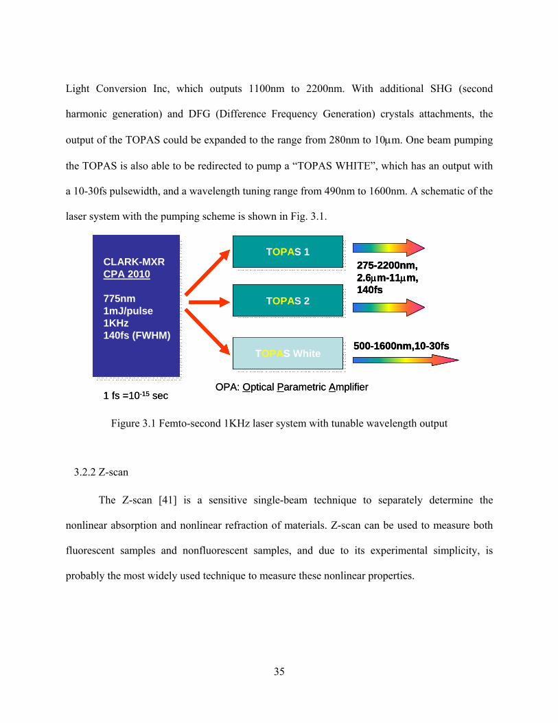
Light Conversion Inc, which outputs 1100nm to 2200nm. With additional SHG (second

harmonic generation) and DFG (Difference Frequency Generation) crystals attachments, the

output of the TOPAS could be expanded to the range from 280nm to 10µm. One beam pumping

the TOPAS is also able to be redirected to pump a “TOPAS WHITE”, which has an output with

a 10-30fs pulsewidth, and a wavelength tuning range from 490nm to 1600nm. A schematic of the

laser system with the pumping scheme is shown in Fig. 3.1.

CLARK-MXRCPA 2010

775nm1mJ/pulse1KHz140fs (FWHM)

TOPAS 1TOPAS 1

TOPAS 2TOPAS 2

TOPAS WhiteTOPAS White

275-2200nm,2.6µm-11µm,140fs

500-1600nm,10-30fs

1 fs =10-15 secOPA: Optical Parametric Amplifier

CLARK-MXRCPA 2010


TOPAS 1TOPAS 1

TOPAS 2TOPAS 2


275-2200nm,2.6µm-11µm,140fs

500-1600nm,10-30fs

CLARK-MXRCPA 2010


TOPAS 1TOPAS 1

TOPAS 2TOPAS 2


275-2200nm,2.6µm-11µm,140fs

500-1600nm,10-30fs

1 fs =10-15 secOPA: Optical Parametric Amplifier

Figure 3.1 Femto-second 1KHz laser system with tunable wavelength output

3.2.2 Z-scan

The Z-scan [41] is a sensitive single-beam technique to separately determine the

nonlinear absorption and nonlinear refraction of materials. Z-scan can be used to measure both

fluorescent samples and nonfluorescent samples, and due to its experimental simplicity, is

probably the most widely used technique to measure these nonlinear properties.

35

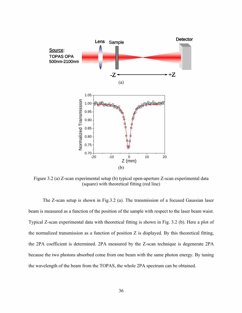
Source:TOPAS OPA500nm-2100nm

Detector

+Z-Z

Lens Sample


Detector

+Z-Z

Lens


Detector

+Z-Z

Lens Detector

+Z-Z

Lens Sample

(a)

-20 -10 0 10 200.70

0.75

0.80

0.85

0.90

0.95

1.00

1.05

Nor

mal

ized

Tra

nsm

issi

on

Z (mm) (b)

Figure 3.2 (a) Z-scan experimental setup (b) typical open-aperture Z-scan experimental data (square) with theoretical fitting (red line)

The Z-scan setup is shown in Fig.3.2 (a). The transmission of a focused Gaussian laser

beam is measured as a function of the position of the sample with respect to the laser beam waist.

Typical Z-scan experimental data with theoretical fitting is shown in Fig. 3.2 (b). Here a plot of

the normalized transmission as a function of position Z is displayed. By this theoretical fitting,

the 2PA coefficient is determined. 2PA measured by the Z-scan technique is degenerate 2PA

because the two photons absorbed come from one beam with the same photon energy. By tuning

the wavelength of the beam from the TOPAS, the whole 2PA spectrum can be obtained.

36

There are assumptions for the Z-scan method and its theoretical fitting: 1) Thickness of

sample should be much smaller than Rayleigh range of focused laser beam, or “thin sample”

assumption, so changes in the beam diameter within the sample due to diffraction can be

neglected. 2) The nonlinear phase shift should be small enough that no change of the beam

profile occurs within the sample.

If the pump beam experiences linear absorption loss (this is the case when the pump

wavelength is moved to be close to the linear absorption edge), ESA could also happen in a Z-

scan experiment. Because both 2PA and ESA are two-photon processes, a single Z-scan using a

single pulsewidth cannot determine which physical process is occuring. However, we can

separate them with time-resolved experiments, such as using a pump-probe setup in Section 3.2.4.

The details will be discussed in Section 3.2.5

The absolute errors associated with the Z-scan technique using the optical source

described here are estimated to be ±15 ∼ 20%.

3.2.3 Two-Photon Fluorescence (2PF) Spectroscopy

Another single beam technique for measuring degenerate 2PA cross section of molecules

is two-photon fluorescence (2PF) spectroscopy, first developed by C. Xu and W. W. Webb in

1996 [42].

In the 2PF technique, we do not measure the transmission of the beam like in the Z-scan.

Instead, we measure fluorescence due to 2PA. Figure.3.3 shows the fluorescent process due to

1PA (a) and 2PA (b). Fluorescent molecules can absorb one photon to reach an excited state S2,

then, through nonradiative processes, decay to the first excited state S1. The fluorescent

molecules can come back to the ground state S0 by releasing a fluorescence photon, and this

37

process is referred to as radiative decay. The molecule can also absorb two photons

simultaneously to reach an excited state, and then through the same decay processes can come

back to the ground state by emitting a fluorescence photon. Because the photon energy of the

emitted photon is higher than that of a single photon absorbed via 2PA, 2PF spectroscopy is also

called up-conversion fluorescence spectroscopy. By measuring the photon flux of the

fluorescence with respect to a known standard, we can retrieve the 2PA coefficient or cross

section of 2PA of the molecules [42].

S0

hω

hω

S1

S2

S0

hω

hω

S1

S2

S0

hω

hω

S1

S2

S0

hω

S1

S2

FluorescenceAbsorption

Non-radiative decay

S0

hω

S1

S2

FluorescenceAbsorption

Non-radiative decay

(a) (b)

Figure 3.3 Fluorescence following one-photon absorption (a) and two-photon absorption (b)

The experimental setup is shown in Fig.3.4, where a λ/2 WP is a half wave plate, P is a

GLAN-Laser calcite Polarizer. We use them to control the energy and polarization of the input

beam. We use the telescope made of lenses L1 and L2 to expand the beam by 4×, use the iris A2

to truncate the beam and only allow the central part of the beam to reach the focusing lens L3.

By doing this, the spatial profile of the beam on the focusing lens L3 is independent of the pump

wavelength from the TOPAS (usually the spatial profile of the beam from the TOPAS changes

when tuning the wavelength). Thus, the spatial profile of the beam on L3 will be nearly a flat top

beam, so that the intensity distribution at the focal spot after L3 will be a diffraction-limited Airy

38

pattern, which will be considered in the calculation of the fluorescence due to 2PA shown below

[42]. Fluorescent samples experience 2PA at the focal spot to emit fluorescence. Fluorescence is

collected by lens L4 and detected by a photomultiplier tube (PMT). The PMT is very sensitive

detector, allowing 2PF spectroscopy to be a very sensitive method to measure the molecules’

2PA cross section with values even smaller than 1GM. Also, the concentration of the solution

can be less than 10-4 M.

Sample

Fluorescence

λ/2WP P

Mono-chrometer

PMTPC

Source:

L1

L2

A1

A2

L3

L4

Fluorescence

Sample

TOPAS

λ/2WP P

Mono-chrometer

PMTPC

Source:

Fluorescence

Sample

λ/2WP P

Mono-chrometer

PMT

TOPAS

PC

Source:

L1

L2

A1

A2

L3

L4

TOPAS

Figure 3.4 Experimental setup for two-photon fluorescence spectroscopy using femtosecond laser pulses from the TOPAS

There are two separate PMT detectors available covering the different spectral ranges

(R928, 250-800nm; P1524, 250-700nm). The detectors are operated in the analog mode (DC

voltage output) for 2PF measurements. The dynamic range of the PMTs is limited to between

0.03-3 Volts in order to operate in the linear regime of the detector. The fluorescence spectrum is

corrected for the spectral responsivity of the fluorimeter (monochrometer and PMT), and then

39

integrated over the entire emission range to obtain the total integrated fluorescence for a certain

excitation wavelength.

In order to determine the 2PA cross section of molecules, we have to determine the

photon flux of fluorescence based on the spatial and temporal distribution of the pump beam at

the focal point. Here I gave a brief description of this calculation. More details can be found in

Ref. [42].

It is known that the number of photons absorbed per molecule per unit time by 2PA is

proportional to the 2PA cross section δ and to the square of the incident intensity, I [43]. So the

time-averaged fluorescence photon flux )(tF is measured as:

∫=V

dVStICgtF )()(21)( 22

0 rδφη (3.3)

where and describe the spatial and temporal distribution of the incident light at the

focal spot respectively.

)(rS )(0 tI

η is the fluorescence quantum yield of the molecule, and φ is the

fluorescence collection efficiency of the fluorimeter. C is the concentration of the solution.

20

20 )()( tItIg = is a measure of the second-order temporal coherence of the excitation

source. δ is the 2PA cross section of the molecule.

If we assume the spatial profile of the pump beam is a flat-top beam at the focus of lens

L3, we have the time averaged fluorescence photon flux )(tF as:

πλτ

δφη2)(8

21)(

tPnfg

CtF p≈ (3.4)

40

where is the pulse repetition rate, f τ is the pulsewidth (FWHM), )( τfgg p ×=

(22/1

2/1

20

2/1

2/1

20 )()( ⎥⎦

⎤⎢⎣⎡= ∫∫ −−

f

f

f

fp tIdttIg τ ) is equal to 0.664 for a Gaussian temporal profile pulse

and 0.558 for a hyperbolic-secant squared pulse. Equation (3.4) is valid for thick samples where

the sample thickness is much greater than the focal depth. The time averaged fluorescence

photon flux )(tF is the signal detected by the PMT in the analog mode.

We can see in Eq. (3.4) that the 2PF signal 2)()( tPtF ∝ . We can check this quadratic

power dependence of the fluorescence signal to determine that the fluorescence signal detected is

only due to 2PA, not to 1PA or other higher order absorption processes.

From Eq. (3.4), we can see that )(tF is proportional to the 2PA cross section δ and

inversely proportional to the pulsewidth τ and wavelength λ , or τλ

δ 1)( ∝tF . If other

experimental conditions are the same for all excitation wavelengths used (such as collection

coefficient φ , power )(tP ), knowing the 2PA cross section 1δ and fluorescence signal ( )1)(tF

for one excitation wavelength 1λ , we can approximately estimate the 2PA cross section 2δ for

any other excitation wavelength 2λ by the relation:

111

22212 )(

)(λτλτ

δδtFtF

= (3.5)

We use this method when there is no standard molecule available for the excitation wavelength

range.

Based on the Eq. (3.4), we use a relative method to determine the 2PA cross section Sδ

of the sample by using standard reference molecules with known 2PA cross sections, Rδ . We

41

measure the 2PF signal for both the reference molecules and the unknown sample under the

same excitation wavelength. Using Eq. (3.4), we can eliminate the 2PA cross section dependency

on the spatial and temporal profile of the excitation light and the 2PA cross section of an

unknown sample Sδ can be obtained as:

R

SSSSR

RRRRSS

tPCtF

tPCtFδ

ηφ

ηφδ 2

2

)()(

)()(= (3.6)

where the subscripts S and R refer to the sample and reference respectively. The reference

standard molecules we used are: Fluorescein in water (PH=11, quantum yield = 0.9) [42], and

Rhodamine B in methanol (quantum yield=0.7) [42]

For the reference molecules and the unknown sample, the difference of the collection

efficiencies is mainly due to different slit widths W used for the emission monochrometer,

indicated by the micrometer installed on it. The collection efficiency is proportional to the square

of this slit width, [39]. 2W∝φ

Another factor affecting the collection efficiency is the refractive index of solutions.

Usually the collection efficiency can be expressed as ndisp φφφ ×= [13]. dispφ is the collection

efficiency related to the fluorescence spectrum range and corresponding PMT’s response to this

range. And (n is refractive index of the solution) takes into account the difference in the

solid angles under which the illuminated portion of the solution is seen from the PMT, when the

solvents for the reference and the sample are different. This effect is usually considered when the

fluorescence quantum yield is measured. However in our 2PF experimental setup, the excitation

beam is directed close to one side of the cuvette window and the fluorescence emitted passes

through a negligible amount of solvent. Therefore this factor is normally neglected.

2−∝ nnφ

42

We can determine the fluorescence quantum yield of the sample by linear spectroscopy.

In 2PF spectroscopy, we assume the fluorescence quantum yield due to 1PA and 2PA are the

same. We also assume that the fluorescence spectrum due to 1PA and 2PA are identical.

There is another issue we need to deal with, called the inner filter effect, indicating

significant reabsorption of the emission beam because we use relatively high concentrated

solutions (∼ 10-4 M). We measure the one-photon fluorescence spectrum with very low

concentration solutions (peak OD < 0.1 in a 1cm cuvette) by linear spectroscopy, and then

correct the fluorescence spectrum due to 2PA with this one-photon fluorescence spectrum.

Details are described in Ref [28]

The absolute errors associated with this characterization technique are estimated to be

±20%.

3.2.4 White-Light Continuum Pump-Probe Spectroscopy

The two-beam technique we used to measure 2PA is White-Light Continuum (WLC)

pump-probe spectroscopy [44][45]. With this pump-probe technique, we are not only able to

measure nondegenerate 2PA of materials, but we can also study the dynamics of the nonlinearity

in the time regime. For the weak probe beam we can detect additional absorption of the probe

due to nondegenerate 2PA (one photon from the pump, the other photon from the probe) with the

presence of the strong pump beam to determine the 2PA spectra of samples. The pump beam and

probe beam overlap in space and in time (by adjusting the temporal delay) at sample. We can

also use the strong pump pulse to induce the nonlinearity within the sample and the weak probe

pulse monitors the dynamics of that nonlinearity – again by adjusting the temporal delay. Since

43

we use ultrashort pump and probe pulses (∼140fs), we can distinguish the “short-lived” processes

(such as 2PA) from the “long-lived” processes (such as excited state absorption).

Pump-probe experimental setup is shown in Fig.3.5

CCD

λ/2 P

λ/2 P CaF2

BSRR

BS

Delay

P

From TOPAS 2

From TOPAS 1

Pump

WLC-probe

reference

signal

Spectrometer

Sample

CCD

λ/2 P

λ/2 P CaF2

BSRR

BS

Delay

P

From TOPAS 2

From TOPAS 1

Pump

WLC-probe

reference

signal

SpectrometerCCD

λ/2 P

λ/2 P CaF2

BSRR

BS

Delay

P

From TOPAS 2

From TOPAS 1

Pump

WLC-probe

reference

signal

Spectrometer

Sample

Figure 3.5 Experimental setup for white-light continuum pump-probe nonlinear spectroscopy. BS-Beam Splitter, λ/2-half waveplate, P-polarizer, RR-retroreflector

In this White-Light Continuum (WLC) pump probe spectroscopy, in order to generate the

WLC probe beam, we focus a 140fs (FWHM), 2-3 µJ, 1300nm beam from the TOPAS into a

2.5mm thick CaF2 window with a 5cm focal length lens. According to research by Brodeur and

Chin [46], the spectral broadening of the WLC or supercontinuum scales as the bandgap energy

of the generation medium, and CaF2 is one of the transparent media with the largest bandgap

(Egap=10.2eV). The spectral range of the WLC generated by this method is from 400nm to

1600nm.

44

With 140fs pulse excitation, the duration of the WLC probe pulse is much longer than

140fs due to group velocity dispersion (GVD) of the broad WLC spectrum in CaF2. In order to

characterize the temporal properties of the WLC probe, we perform an Optical Kerr Effect (OKE)

pump-probe experiment [44]. The OKE method is a cross-correlation technique used to fully

characterize the chirp of the WLC (relation between the wavelength and time) and furthermore

can measure the GVD of an unknown sample. More details can be found in Ref [44]. The

duration of the WLC is around 2ps with 1600nm at the front in time and 400nm toward the back

(i.e. normal dispersion).

Nondegenerate 2PA requires that the pump and probe pulses reach the sample at the same

time. The single wavelength pump pulse from another TOPAS has a duration of ~140fs, much

shorter than the WLC probe. Thus it is necessary to scan the temporal delay of the pump pulse to

reach zero delay with different wavelength components of the WLC probe, i.e. only a narrow

spectral portion of the WLC undergoes 2PA for a fixed temporal delay.

In addition, photons from the pump and WLC probe have different wavelengths so that

they travel at different speeds inside the sample. This causes temporal walk off making the

effective interaction length in the sample between the pump and probe pulses to be significantly

reduced. Thus, the magnitude of the nonlinear signal will be reduced as well. Therefore,

experimentally determined raw data is corrected for this temporal walk off due to group-velocity

mismatch (GVM). GVM can be completely corrected for provided the linear dispersion of the

sample is known. We can characterize the dispersion of the sample by the OKE method

mentioned above.

We derived a single dynamical equation to describe the transmission of the WLC probe

due to nondegenerate 2PA including the walk-off correction as [44]:

45

( ) ( )[ ] τρττρ

πρττπ

ρτσσ

derferfWW

eWQ dd ∫

∞+

∞−

−

⎪⎭

⎪⎬⎫

⎪⎩

⎪⎨⎧

−−Γ

−⎟⎠⎞

⎜⎝⎛ −+

−=Γ22

exp),,,,( (3.7)

where Q is the transmission of the WLC probe, σ is the linear absorption coefficient, τd is the

delay time between the pump and probe pulses, and W is the ratio of the band-limited probe

pulsewidth to pump pulsewidth. ρ is the parameter related to the GVM between pump and probe

pulses. Γ is the parameter related to the nondegenerate 2PA coefficient; NDeLI β=Γ , here L is

the sample length and Ie is the pump beam intensity.

3.2.5 Pump-probe experiments to study ESA and 2PA processes

In order to investigate 2PA bands located at high energy (or shorter wavelength) region

where the large 2PA cross sections usually could be observed, we have to use the pump

wavelengths as short as possible, i.e. move the pump wavelength close to longer wavelength

edge of linear absorption band. Therefore, pump light might experience some linear absorption.

In the Z-scan experiment. as discussed in Section 3.2.4, If the pump beam experiences linear

absorption, excited state absorption (ESA) could also happen. Because both 2PA and ESA are

two-photon processes, a single wavelength Z-scan using a single pulsewidth cannot determine

which physical process is occurring. However, we can separate them with time-resolved

experiments, such as using a white-light continuum pump-probe setup in Section 3.2.4. Because

ESA and 2PA have different time responses, ESA shows a longer time response (usually

hundreds of ps to ns) than 2PA (which is essentially “instantaneous”)

1) Let’s see the case of the molecule TOR-I-103. The molecular structure and 2PA data

for this molecule are presented in Section 5.4. The peak 2PA cross sections are observed to be ≈

34000 GM at 515nm correponding pump wavelength 1030nm with Z-scan technique. The time-

46

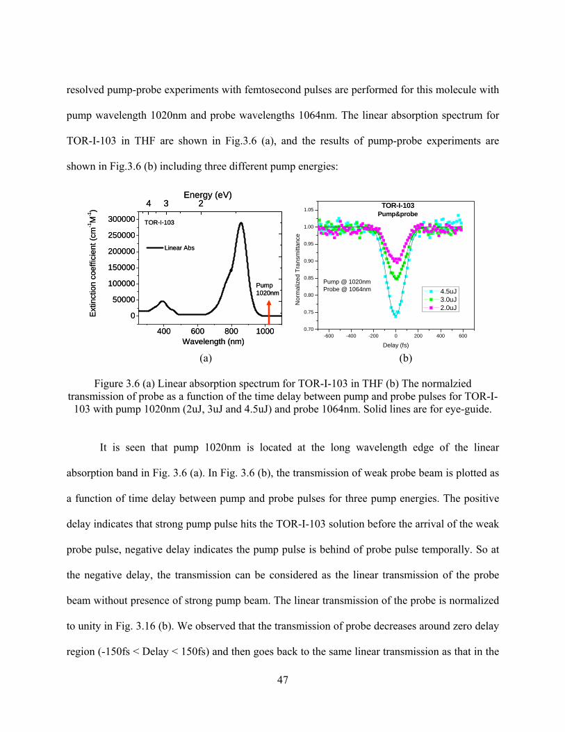
resolved pump-probe experiments with femtosecond pulses are performed for this molecule with

pump wavelength 1020nm and probe wavelengths 1064nm. The linear absorption spectrum for

TOR-I-103 in THF are shown in Fig.3.6 (a), and the results of pump-probe experiments are

shown in Fig.3.6 (b) including three different pump energies:

400 600 800 1000

0

50000

100000

150000

200000

250000

300000 TOR-I-103

Ext

inct

ion

coef

ficie

nt (c

m-1M

-1)

Wavelength (nm)

Linear Abs

4 3 2Energy (eV)

Pump 1020nm

400 600 800 1000

0

50000

100000

150000

200000

250000

300000 TOR-I-103

Ext

inct

ion

coef

ficie

nt (c

m-1M

-1)

Wavelength (nm)

Linear Abs

4 3 2Energy (eV)

Pump 1020nm

-600 -400 -200 0 200 400 6000.70

0.75

0.80

0.85

0.90

0.95

1.00

1.05

Nor

mal

ized

Tra

nsm

ittan

ce

Delay (fs)

4.5uJ 3.0uJ 2.0uJ

TOR-I-103Pump&probe

Pump @ 1020nmProbe @ 1064nm

(a) (b)

Figure 3.6 (a) Linear absorption spectrum for TOR-I-103 in THF (b) The normalzied transmission of probe as a function of the time delay between pump and probe pulses for TOR-I-

103 with pump 1020nm (2uJ, 3uJ and 4.5uJ) and probe 1064nm. Solid lines are for eye-guide.

It is seen that pump 1020nm is located at the long wavelength edge of the linear

absorption band in Fig. 3.6 (a). In Fig. 3.6 (b), the transmission of weak probe beam is plotted as

a function of time delay between pump and probe pulses for three pump energies. The positive

delay indicates that strong pump pulse hits the TOR-I-103 solution before the arrival of the weak

probe pulse, negative delay indicates the pump pulse is behind of probe pulse temporally. So at

the negative delay, the transmission can be considered as the linear transmission of the probe

beam without presence of strong pump beam. The linear transmission of the probe is normalized

to unity in Fig. 3.16 (b). We observed that the transmission of probe decreases around zero delay

region (-150fs < Delay < 150fs) and then goes back to the same linear transmission as that in the

47

negative delay. We can conclude that the probe transmission “instantaneous” change around zero

delay region is due to nondegenerate 2PA (one photon from pump, the other photon from probe).

There is no ESA occurring for this case. We can trust the signal we see in the single wavelength

Z-scan experiment with pump 1030nm is from the pure 2PA process.

2) Let’s look at the case for molecule Sjz-3-16 in THF. The spectroscopic data for this

molecule can be found at Appendix C.3. The linear absorption spectrum of Sjz-3-16 in THF is

shown in Fig. 3.7 (a), and the pump probe data in Fig. 3.7 (b) and (c)

Pump 600nm is located at edge of linear absorption band of Sjz-3-16 in THF shown in

Fig. 3.7 (a). In Fig 3.7 (b), at after delay ≈ 150 fs, the transmission of weak probe beam is

smaller than normalized linear transmission at negative delay, and staying almost same for the

delay up to 1.4 ps. We can conclude that this decrease of transmission of the probe (∆) after zero-

delay region (-150fs – 150fs) is because of ESA, which is evidenced by its long time response

behavior (usually hundreds ps to ns). In addition, the dip of the probe transmission at zero delay

have contributions both from the non-degenerate 2PA and ESA.

Because the strong pump 600nm femtosecond pulse may experience both 2PA and 1PA.

In order to tell which absorption process dominates here, we plot the logarithm of ESA signal (∆)

as a function of logarithm of pump energy and fit the experimental data with linear function in

Fig. 3.7 (c). The relationship of 1PA and 2PA induced electron population of first excited state

N1 that is responsible to ESA without considering lifetime of the excited state can be expressed

as:

ωβ

ωα

hh 2)()( 2

1 tItIdt

dN+= (3.8)

48

Where α is 1PA coefficient, β is 2PA coefficient, I(t) is irradiance of pump beam and ωh is

pump photon energy. In Fig 3.7 (c), the slope of 1.1 is observed to indicates that 1PA dominates

here, and ESA signal is mainly due to 1PA of pump beam. So if we use 600nm as the pump

beam in single wavelength open-aperture Z-scan experiment, the signal we see is due to 2PA

plus 1PA followed with ESA, even although the Z-scan signal can be well fitted with 2PA theory.

300 400 500 600 7000

20000

40000

60000

80000

100000

Ext

inct

ion

coef

ficie

nt (c

m-1M

-1)

Wavelength (nm)

Linear Abs

4 3.5 3 2.5 2

Sjz-3-16

Energy (eV)

Pump 600nm

300 400 500 600 7000

20000

40000

60000

80000

100000

Ext

inct

ion

coef

ficie

nt (c

m-1M

-1)

Wavelength (nm)

Linear Abs

4 3.5 3 2.5 2

Sjz-3-16

Energy (eV)

Pump 600nm

300 400 500 600 7000

20000

40000

60000

80000

100000

Ext

inct

ion

coef

ficie

nt (c

m-1M

-1)

Wavelength (nm)

Linear Abs

4 3.5 3 2.5 2

Sjz-3-16

Energy (eV)

Pump 600nm

0.4 0.5 0.6 0.7 0.8 0.9 1.0

-1.5

-1.4

-1.3

-1.2

-1.1

-1.0

-0.9 Linear Fitslope=1.1

log

(∆)

Log(pump energy) (a) (c)

-600 -300 0 300 600 900 1200 1500 18000.6

0.7

0.8

0.9

1.0

1.1 sjz-3-16 in THF, C=4E-3M, pump 600nm, probe 650nm

Tran

smis

sion

Delay (fs)

Pump energy 9uJ 6uJ 3uJ

∆1 ∆2 ∆3

ESA

-600 -300 0 300 600 900 1200 1500 18000.6

0.7

0.8

0.9

1.0


Tran

smis

sion

Delay (fs)


∆1 ∆2 ∆3

-600 -300 0 300 600 900 1200 1500 18000.6

0.7

0.8

0.9

1.0


Tran

smis

sion

Delay (fs)


∆1 ∆2 ∆3

ESA

(b)

Figure 3.7 (a) Linear absorption spectrum of Sjz-3-16 in THF; (b) The normalized transmission of probe 650nm as a function of the time delay between pump and probe pulses for Sjz-3-16 with

pump 600nm (3uJ, 6uJ and 9uJ) and probe 650nm. ESA signals are indicated by ∆1, ∆2 and ∆3 for three pump energies respectively; (c) Plot of logarithm of ESA signal (∆) as a function of

logarithm of pump energy

49

3) In addition, let’s look at the case for LB-II-80 in THF. The spectroscopic data are

shown in Appendix C.3. The linear absorption spectrum of LB-II-80 in THF is shown in Fig. 3.8

(a), and the pump probe data in Fig. 3.8 (b) and (c)

300 400 500 600 700

0

20000

40000

60000

80000

100000

120000 LB-II-80

Ext

inct

ion

coef

ficie

nt (c

m-1M

-1)

Wavelength (nm)

Linear Abs

4 3.5 3 2.5 2

Energy (eV)

Pump 600nm

300 400 500 600 700

0

20000

40000

60000

80000

100000

120000 LB-II-80

Ext

inct

ion

coef

ficie

nt (c

m-1M

-1)

Wavelength (nm)

Linear Abs

4 3.5 3 2.5 2

Energy (eV)

300 400 500 600 700

0

20000

40000

60000

80000

100000

120000 LB-II-80

Ext

inct

ion

coef

ficie

nt (c

m-1M

-1)

Wavelength (nm)

Linear Abs

4 3.5 3 2.5 2

Energy (eV)

Pump 600nm

-0.6 -0.3 0.0 0.3 0.6 0.9 1.2

-3.0-2.7-2.4-2.1-1.8-1.5-1.2-0.9-0.6

Linear Fitslope=1.4

Log

(∆)

Log (Pump energy)

(a) (c)

-600 -300 0 300 600 900 1200 1500 1800

0.4

0.5

0.6

0.7

0.8

0.9

1.0

LBII80 in THFpump 600nm probe 550nm

Tran

smis

sion

Delay (fs)

Pump energy 9uJ 6uJ 3uJ 1uJ 0.5uJ

∆3

∆4∆5

ESA

-600 -300 0 300 600 900 1200 1500 1800

0.4

0.5

0.6

0.7

0.8

0.9

1.0


Tran

smis

sion

Delay (fs)


∆3

∆4∆5

-600 -300 0 300 600 900 1200 1500 1800

0.4

0.5

0.6

0.7

0.8

0.9

1.0


Tran

smis

sion

Delay (fs)


∆3

∆4∆5

ESA

(b)

Figure 3.8 (a) Linear absorption spectrum of LB-II-80 in THF; (b) The normalized transmission of probe 550nm as a function of the time delay between pump and probe pulses for LB-II-80

with pump 600nm. ESA signals are indicated by ∆3, ∆4 and ∆5 for pump energies 3uJ, 6uJ and 9uJ respectively. ESA signals for pump enegies 0.5uJ and 1uJ are equal to ∆1 = 0.002, ∆2 =

0.005 respectively (not shown in the graph); (c) Plot of logarithm of ESA signal (∆) as a function of logarithm of pump energy.

50

The pump 600nm is located quite close to linear absorption band for LB-II-80 in THF

shown in Fig. 3.8 (a). ESA with probe 550nm is observed for all the pump energies shown in Fig.

3.8 (b). In Fig 3.8 (c), Slope is equal to 1.4 indicates that ESA have contributions from both 2PA

and 1PA of pump 600nm according to Eq. (3.8), i.e. pump 600nm beam experiences both 1PA

and 2PA here.

4) We performed the pump-probe experiment for LB-II-80 in THF with another pump

wavelength 690nm that is far from linear absorption edge shown in Fig. 3.9 (a), therefore

experiences negligible 1PA. The pump probe data in Fig. 3.9 (b) and (c), non-smooth curves in

Fig. 3.9 (b) are due to the crosstalk between motor cable and detector cables.

Shown in Fig. 3.9 (b), ESA is observed for all the pump energies, and the slope in Fig.

3.9 (c) is observed to be equal to 2.15, which indicates that here 2PA dominates absorption

process for strong pump 690nm. Here ESA is mainly due to 2PA, i.e. a three-photon process. If

we use pump 690nm in the single wavelength Z-scan experiment, we prefer to use smaller pump

energy to minimize higher order ESA+2PA effect. If pump energy is high, Z-scan signal will not

be able to be fitted with pure 2PA theory.

51

300 400 500 600 700

0

20000

40000

60000

80000

100000

120000 LB-II-80

Ext

inct

ion

coef

ficie

nt (c

m-1M

-1)

Wavelength (nm)

Linear Abs

4 3.5 3 2.5 2

Energy (eV)

Pump 690nm

300 400 500 600 700

0

20000

40000

60000

80000

100000

120000 LB-II-80

Ext

inct

ion

coef

ficie

nt (c

m-1M

-1)

Wavelength (nm)

Linear Abs

4 3.5 3 2.5 2

Energy (eV)

Pump 690nm

0.6 0.7 0.8 0.9 1.0 1.1 1.2-2.4

-2.2

-2.0

-1.8

-1.6

-1.4

-1.2 Linear Fitslope=2.15

Log

(∆)

Log (pump energy) (a) (c)

-600 -300 0 300 600 900 1200 1500 1800

0.87

0.90

0.93

0.96

0.99

1.02LB-II-80 in THFpump 690nm, probe 750nm

Tran

smis

sion

Delay (fs)

Pump energy 13uJ 10uJ 7uJ 3uJ

∆1

∆2∆3

∆4

ESA

-600 -300 0 300 600 900 1200 1500 1800

0.87

0.90

0.93

0.96

0.99


Tran

smis

sion

Delay (fs)


∆1

∆2∆3

∆4

-600 -300 0 300 600 900 1200 1500 1800

0.87

0.90

0.93

0.96

0.99


Tran

smis

sion

Delay (fs)


∆1

∆2∆3

∆4

ESA

(b)

Figure 3.9 (a) Linear absorption spectrum of LB-II-80 in THF; (b) The normalized transmission of probe 750nm as a function of the time delay between pump and probe pulses for LB-II-80

with pump 690nm. ESA signals are indicated by ∆1, ∆2, ∆3 and ∆4 for pump energies 3uJ, 7uJ, 10uJ and 13uJ respectively. (c) Plot of logarithm of ESA signal (∆) as a function of logarithm of

pump energy

52

CHAPTER 4 STRUCTURE-PROPERTY RELATIONSHIP OF POLYMETHINE DYES

4.1 Cyanines

The generic cyanine dyes consist of two nitrogen centers, one of which is positively

charged and is linked by a conjugated chain of a number of carbon atoms to the other nitrogen.

For example, the structures of PDs are shown in Fig. 4.1.Both polymethine dyes and squaraine

dyes belong to the family of cyanine dyes. Polymethine dyes are also called cationic

streptopolymethine-cyanines, and squaraine dyes are referred as Zwitterionic squaraine-based

cyanine dyes. In this chapter, we will discuss relationships of molecular structure to linear and

nonlinear optical properties for polymethine dyes. The squaraine dyes will be discussed in

Chapter 5.

In the middle of the 19th century, cyanine dyes were first used as the spectral sensitizers

for silver halide photography, and dominate the field of photography since then [47]. Although

polymethine and squaraine dyes are substances with a variety of colors in solution, they are not

widely used for dyeing purposes because they are decolorized by light and acid, i.e. bleached.

However, they have been widely used in optical disks as recording media [48], saturable

absorbers for Q-switching and modelocking [49], and gain media in dye lasers [50]. Cyanines are

also used for initiation of photopolymerization, as molecular probes in polymer science and

biology [51], as nonlinear media for exploring excited-state absorption [52] [53]. Polymethine

molecules are also useful objects for developing new theoretical concepts and effective quantum-

chemical models.

53

4.2 Polymethine dyes

The name polymethine refers to the π conjugated chromophore chain, which is composed

of the methine groups and serves as a light absorbing chromophore of the molecule. The general

structure of a polymethine dye (PD) is shown in Fig. 4.1(a), where R1 and R2 represent terminal

groups. PDs are a special type of the charged (ionic) linear π-electron conjugated system.

R1N NR2n

+

δ+ δ+ δ+

δ- δ-R1N +NR2

δ+ δ+ δ+

δ- δ-R1N +NR2

(a) (b)

Figure 4.1 (a) General molecular structure of PD, R1 and R2 are terminal groups; (b) π-electron distribution in polymethine chromophore.

The key feature of the polymethine chromophore is an alternating partial charge (δ+ and

δ- are positive and negative charge, respectively) at the carbon atoms within the polymethine

chain along with an equalization of the bond lengths as shown in Fig.4.1(b). This property allows

a large delocalization of the π-electron system, which gives rise to a large polarizability and

promises a strong nonlinear interaction upon excitation.

Altering the chromophore via the addition of terminal groups to the two end positions

gives us the ability to generate different chemical archetypes by affecting the electron accepting

and donating properties of the system. By placing the terminal groups with high (accepting) or

low (donating) electron affinities we can create the following motifs: 1) Donor-π conjugated

chromophore-Donor (D-π-D), 2) Donor-π conjugated chromophore-Acceptor (D-π-A). We can

also control the strength of these electron accepting/withdrawing terminal groups, which gives us

54

further freedom to address the effect these structural changes having on the molecule’s NLO

properties.

Polymethine dyes (PDs) have highly intense and comparatively narrow absorption and

fluorescence bands which can be shifted from the visible to infrared (>1600nm) region by

lengthening the polymethine chain (up to n=13) [54] or by introducing specific terminal groups.

The PDs we studied in this thesis are shown in Fig. 4.2:

NN

CH3 CH3

CH3CH3

+

ClO4-

N

CH3CH3

CH3

N

CH3

CH3

CH3

BF4-

+PDAF

PD2350

PD3428

PD824N

CH3CH3

CH3CH3

N

CH3CH3 CH3CH3

CH3CH3

ClO4-

+

I

N

CH3CH3CH3

CH3

C3H7

NC3H7

+

N

SS

NCH3CH3 I-

+

PD25

PD2646

PD2501

S

NC2H5

S

NC2H5

CH3C6H4SO3-

+

S

NCH3

S

NCH3

CH3C6H4SO3

+

-

N

CH3CH3

N

CH3 CH3

C2H5 C2H5

p-CH3C6H4SO3

+

-

PD2630

PD2665 NCH3

CH3CH3S

NC2H5 ClO4

+

-

Styryl_1S

N

NCH3

CH3C2H5

CH3C6H4SO3

+

-

PD2093 C6H5

N

CH3CH3

N

CH3CH3

ClO4

+

-

S

NC2H5

S

NC2H5

CH3C6H4SO3

+

-

PD200

NCH3N

CH3CH3

CH3CH3

+

BF4-

PD2755

NCH3N

CH3

CH3CH3

CH3 CH3ClO4

+

-

PD2761

NN

CH3 CH3

CH3CH3

+

ClO4-

N

CH3CH3

CH3

N

CH3

CH3

CH3

BF4-

+PDAFN

CH3CH3

CH3

N

CH3

CH3

CH3

BF4-

+PDAF

PD2350

PD3428

PD824N

CH3CH3

CH3CH3

N

CH3CH3 CH3CH3

CH3CH3

ClO4-

+

I

N

CH3CH3CH3

CH3

C3H7

NC3H7

+

N

SS

NCH3CH3 I-

+

PD25

PD2646

PD2501

S

NC2H5

S

NC2H5

CH3C6H4SO3-

+

S

NCH3

S

NCH3

CH3C6H4SO3

+

-

N

CH3CH3

N

CH3 CH3

C2H5 C2H5

p-CH3C6H4SO3

+

-

PD2630

PD2665 NCH3

CH3CH3S

NC2H5 ClO4

+

-

Styryl_1S

N

NCH3

CH3C2H5

CH3C6H4SO3

+

-

PD2093 C6H5

N

CH3CH3

N

CH3CH3

ClO4

+

-

S

NC2H5

S

NC2H5

CH3C6H4SO3

+

-

PD200

NCH3N

CH3CH3

CH3CH3

+

BF4-

PD2755

NCH3N

CH3

CH3CH3

CH3 CH3ClO4

+

-

PD2761

Figure 4.2 Molecular structures of Polymethine Dyes (PDs)

55

The photochemical stability of PDs degrades as the chain length is increased from the

lowest cyanine limit (n=0) to the carbocyanine (n=1) and on to the di- (n=2), tri-, etc.

carbocyanine structures. It should be noted that much work has been spent on making this series

of dyes photochemically stable [52], with the exception of the pentacarbocyanine dyes which

were only recently synthesized.

PDs are attractive for 2PA due to three advantages: 1) they show large ground-state

transition dipole moments; 2) they have close to parallel orientation of their ground- and excited-

state transition dipole moments [55]; 3) the sharp low-energy side of their linear absorption

spectra allows significant intermediate state resonance enhancement of the 2PA [56]

Linear properties such as peak linear absorption wavelength, λabsmax and fluorescence

spectra peak wavelength λflumax, quantum yield η and peak extinction coefficient εmax of the

polymethine dyes studied in ethanol are summarized at Table 4.1 below:

Table 4.1 Linear optical properties of polymethine dyes in ethanol PD λabs (nm) λflu (nm) η εmax (cm-1 M-1) AF 547 566 0.035 149000

2350 649 665 0.38 235000 3428 756 - - 292000 2093 771 - - 294000 824 863 - - 224000 25 560 572 0.063 151000 200 648 670 0.0656 160000 2646 654 675 0.3 240000 2501 762 788 - 228000 2630 682 704 - 211900

Styryl 1 527 598 0.013 61500 2665 644 667 0.243 197000 2755 570 605 0.066 168500 2761 536 553 0.11 250200

56

4.3 Symmetry

It is well known that materials with symmetry through their center of inversion have

ground and excited states with a definite parity. These materials are referred to as centro-

symmetric systems. Their states are usually separated as symmetric or unsymmetric states.

Quantum mechanics dictates that in centro-symmetric systems, linear excitation and two-photon

excitation processes access states of differing parity. One-photon absorption will gain access to a

state which is opposite in symmetry to that of the ground state, whereas 2PA will access a state

of like symmetry [57][58] [59].

We consider the effect of molecular symmetry on 2PA by comparing results for the

symmetrical PD 2350 (indolium terminal groups, n = 2) with the weakly asymmetrical PD 2665

(indolium – thiazolium terminal groups, n = 2), and also with the strong asymmetrical molecule

PD2755 (indolium-terminal groups, n=2).

Degenerate 2PA spectra of these molecules in ethanol were taken by using 2PF

spectroscopy and the Z-scan technique. Experimental results and theoretical fittings based on Eq.

(2.55) in chapter 2 are shown in Fig. 4.3. Here the two-photon absorption cross section δ is

plotted versus half the wavelengths of the input photons. The 2PA cross-section is a unit

expressed in 10-50 cm4*sec/photon that is defined as Goppert-Mayer (GM).

It is commonly known that asymmetrical dyes are characterized by blue-shifted and

broader linear absorption bands S0 → S1 as compared to those for symmetrical dyes. We can see

this in Fig. 4.3 where the solid lines indicate linear absorption spectra. Absorption shapes for

asymmetrical molecules strongly depend on solvent polarity which is connected to the charge

localization [55].

57

PD 2350 PD 2665 PD 2755

N

CH3

CH3

C3H7

NC3H7

CH3

CH3

I

+N N

S

CH3

CH3CH3

C2H5 ClO4

+

-N

CH3

CH3

N

CH3

CH3

CH3

+

BF4-

PD 2350 PD 2665 PD 2755

N

CH3

CH3

C3H7

NC3H7

CH3

CH3

I

+N N

S

CH3

CH3CH3

C2H5 ClO4

+

-N

CH3

CH3

N

CH3

CH3

CH3

+

BF4-

(a)

300 400 500 600 700

0200400600800

100012001400

2PA

cro

ss s

ectio

n δ

(GM

)

Wavelength (nm)

PD2665 PD2350 PD2755

0

50000

100000

150000

200000

250000

Ext

inct

ion

coef

ficie

nt (c

m-1M

-1)

4 3 2Energy (eV)

(b)

Figure 4.3 (a) Molecular structures (b) Degenerate 2PA spectra for PD2350 (red), PD2665 (black) and PD2755 (blue). Dashed line is the theoretical fitting based on Eq. (2.55), and the linear

absorption spectra (solid line) are shown for reference.

2PA spectra also show some differences. As was expected, for the strongly asymmetrical

PD2755, the first 2PA band is much broader than that for the symmetrical PD 2350; however,

δ2PA for the second band is smaller. The same, but less pronounced effect was observed for the

weakly asymmetrical PD 2665 when compared to the symmetrical PD 2350. We note that for PD

2665 the beginning of the third 2PA band is observed while this is not the case for the

symmetrical PD 2350. PD2350, a symmetric dye, shows negligible 2PA into the peak of the first

singlet excited state, but displays a first 2PA band corresponding to its vibration shoulder due to

58

the effect of vibronic coupling partly breaking the molecular symmetry. We will discuss the

nature of symmetry breaking in Chapter 5 and 6.

We also compare results for the symmetrical molecule PD 25 (thiazolium terminal groups,

n = 1) with the strongly asymmetrical molecule Styryl 1 (thiazolium – styryl terminal groups, n =

1). Molecular structures and experimental results are presented in Fig.4.4.

PD 25 Styryl_1

S

NC2H5

S

NC2H5

CH3C6H4SO3-

+S

N

NCH3

CH3C2H5

CH3C6H4SO3

+

-

PD 25 Styryl_1

S

NC2H5

S

NC2H5

CH3C6H4SO3-

+S

N

NCH3

CH3C2H5

CH3C6H4SO3

+

-

(a)

300 400 500 6000

50

100

150

200

250

300

2PA

cro

ss s

ectio

n δ

(GM

)

Wavelength (nm)

Styryl_1 PD25

0

30000

60000

90000

120000

150000

Ext

inct

ion

coef

ficie

nt (c

m-1M

-1)

4 3 2Energy (eV)

(b)

Figure 4.4 (a) Molecular structures (b) Degenerate 2PA spectra for PD25 (red), Styryl_1 (black). The dashed line is for theoretical fitting based on Eq. (2.55), and linear absorption spectra (solid

line) are shown for reference.

Styryl_1, a strongly asymmetrical molecule, shows a relatively strong and broad 2PA

band within the linear absorption band when the two-photon absorption cross section δ is plotted

59

versus half the wavelength of the input photons. PD 25 shows a less intense vibrationally

induced 2PA band close to the position of its vibration shoulder.

4.4 Terminal groups

Altering the chromophore of PDs via the addition to the two end groups gives us the

ability to generate different chemical archetypes by affecting the electron accepting and donating

properties of the system. By placing terminal groups (TGs) at these positions with low (donating)

electron affinities we can create the following motifs such as Donor-π conjugated core-Donor

(D-π-D). We can also control the strength of these electron donating end groups which gives us

further freedom to address the effect these structural changes having on the molecule’s NLO

properties.

We consider the effect of the three terminal groups: thiazolium, indolium and

benzoindolium, on the one- and two-photon absorption properties. Fig. 4.5 represents

experimental results for PDs with the same length of the chromophore n = 2 and different

terminal groups placed in order of a decrease of their donor strength: PD 2630 (benzoindolium),

PD 2350 (indolium) and PD 2646 (thiazolium), respectively. Degenerate 2PA spectra of these

molecules in ethanol were taken by using 2PF spectroscopy and Z-scan. Molecular structures are

shown in Fig. 4.5 (a). The 2PA spectra are shown in Fig. 4.5 (b). Here the two-photon absorption

cross section δ is plotted versus half of the wavelengths of the input photons. A summary of

ground state transition dipole moments µ01, calculated excited state transition dipole moments

µ12 (obtained by fitting the 2PA spectra with Eq. (2.55)), as well as maximum 2PA cross sections

δmax, are shown in Table 4.2.

60

PD 2350 PD 2646PD 2630

N

CH3CH3

N

CH3 CH3

C2H5 C2H5

p-CH3C6H4SO3

+

-

N

CH3

CH3

C3H7

NC3H7

CH3

CH3

I

+ S

NCH3

S

NCH3

CH3C6H4SO3

+

-

PD 2350 PD 2646PD 2630

N

CH3CH3

N

CH3 CH3

C2H5 C2H5

p-CH3C6H4SO3

+

-

N

CH3

CH3

C3H7

NC3H7

CH3

CH3

I

+ S

NCH3

S

NCH3

CH3C6H4SO3

+

-

(a)

300 400 500 600 700 8000

300

600

900

1200

1500

2PA

cro

ss s

ectio

n δ

(GM

)

Wavelength (nm)

PD2630 PD2350 PD2646

0

50000

100000

150000

200000

250000

Ext

inct

ion

coef

ficie

nt (c

m-1M

-1)

4 3 2Energy (eV)

(b)

Figure 4.5 (a) Molecular structures; (b) Degenerate 2PA spectra for PD 2630, PD 2350 and PD 2646. The dashed line is for theoretical fitting based on Eq. (2.55), and linear absorption spectra

(solid line) are shown for reference.

Table 4.2 Parameters for PDs having the same conjugate length with benzoindolium (PD2630); indolium (PD2350); thiazolium (PD2646) terminal groups

Molecules µ01(debye) µ12(debye) δmax (GM) ∆E (eV) PD2630 14 3.1 980 0.35 PD2350 15 2.0 720 0.31 PD2646 14 1.5 600 0.29

All linear and nonlinear parameters for PD 2646 and PD 2350 are very close in

accordance with the similar donor strength and similar contribution of π-conjugation from their

terminal groups to the polymethine chain. However, we note that δ2PA in both 2PA bands of PD

2350 is 20-40 % larger than those of PD 2646.

61

For PD 2630, with the larger π-conjugation (larger contribution to the chain) and

increased donor strength in the benzoindolium terminal groups, the positions of the one- and

two-photon absorption peaks are red-shifted, and δ2PA for the second band is ≈ 1.5× larger than

for PD 2646. The 2PA spectrum for PD 2630 is more complicated than for PD 2350. In contrast

to PD 2350, the beginning of the next, third 2PA band, is seen for PD 2630, with δ2PA reaching

1320 GM. Further tuning of the excitation wavelength into the short wavelength region was

restricted by the presence of linear absorption. Quantum chemical calculations related to the

effect of terminal groups will be addressed in Chapter 5.

All three terminal groups we studied here contain their own π-conjugated system, which

will change the effective conjugation length of the molecules. When we discuss the effect of

terminal groups on 2PA properties, besides the strength of donors, we also have to consider the

change of the effective molecular conjugate length due to the terminal groups. From Section 4.5,

we observed the trend that increasing the conjugation length of the molecules leads to an

increase of the ground-state transition dipole moments in Section 4.5. However, we do not see

this trend with different terminal groups (see the Table 4.2). It should be an interesting topic to

study the change of the effective conjugation length due to terminal groups on the 2PA

properties of molecules.

Comparing the 2PA properties of PD 200 and PD 2761 gives us some insights about this.

They have the same length of the chromophore n = 2 and different terminal groups, i.e. TGs for

PD 200 and PD 2761 have similar donor strength but very different conjugation length, which

will make the effective conjugation length of PD 2761 smaller. Both of them have benzene

bridges in the middle of the chromophore chain. Degenerate 2PA spectra of these molecules in

ethanol were also taken by using 2PF spectroscopy and Z-scan. Molecular structures are shown

62

in Fig. 4.6 (a). The 2PA spectra are shown in Fig. 4.6 (b). Here the two-photon absorption cross-

section δ is plotted versus the half of input photon wavelengths. A summary of ground state

transition dipole moment µ01, as well as maximum 2PA cross section δmax are shown in Table 4.3.

PD 200 PD 2761

S

NC2H5

S

NC2H5

CH3C6H4SO3

+

-

NCH3N

CH3

CH3CH3

CH3 CH3ClO4

+

-

PD 200 PD 2761

S

NC2H5

S

NC2H5

CH3C6H4SO3

+

-

NCH3N

CH3

CH3CH3

CH3 CH3ClO4

+

-

S

NC2H5

S

NC2H5

CH3C6H4SO3

+

-

NCH3N

CH3

CH3CH3

CH3 CH3ClO4

+

-

(a)

300 400 500 600 700

0150300450600750900

2PA

cro

ss s

ectio

n (G

M)

Wavelength (nm)

PD2761 PD200

0

50000

100000

150000

200000

250000

Extin

ctio

n co

effic

ient

(cm

-1M

-1)4.5 4 3.5 3 2.5 2

Energy (eV)

(b)

Figure 4.6 (a) Molecular Structure (b) Degenerate 2PA spectra for PD 200 and PD 2761. The dashed line is for theoretical fitting based on Eq. (2.55), and linear absorption spectra (solid line)

are shown for reference

Table 4.3 Parameters for PD 200 and PD 2761 having the same chromophore conjugation length with different terminal groups

Molecules µ01(debye) µ12(debye) δmax (GM) ∆E (eV) PD 200 11 2.2 703 0.32 PD 2761 12.8 1.5 248 0.52

The main difference between PD 2761 and PD 200 is that PD 2761 has a very simplified

terminal group (TG) without conjugation, which will make the effective conjugation length of

63

PD 2761 smaller, and is the reason why the linear absorption band of PD 2761 is so shifted to the

“blue” region. Here we observe that the one-photon absorption band of PD 2761 is blue-shifted

by ∼ 110nm compared to PD 200. This shift is approximately equal to the shift upon lengthening

of the chain by one unit. Thus, this is a manifestation of the conjugation in TG on the linear

properties. The two-photon absorption band is also shifted by a smaller amount ∼ 50nm, which is

also observed for the dyes upon lengthening of the chain by one unit.

It is interesting to observe that PD 2761 shows a smaller peak 2PA cross section. From

the Table 4.3, PD 2761 possesses a larger ground state transition dipole moment than PD 200, a

shorter effective conjugation length, but a much smaller observed 2PA cross section. This could

be considered as evidence that π-conjugation in TG of PD 200 improves the 2PA probability by

increasing the excited state absorption dipole moments and decreasing the detuning energy

shown in Table 4.3. It is noticable that extending π-conjugation in chromophore chain of

polymethine will increase 2PA cross setions by increasing ground state transition dipole

moments shown in Section 4.5

4.5 Conjugation length

For symmetric molecules the first accessible two-photon state is 2A1 (numbering is the

following: Ag only for the neutral molecules like polyenes and squaraine dyes, and A1 for

polymethine dyes) corresponds to the second singlet excited state. Based on perturbation theory

for a three-state model having one-intermediate state for 2PA shown in Chapter 2, the dominant

terms which affect the two-photon properties of this transition are the ground to first excited state

(intermediate state) with the transition dipole moment µ01 as well as the first to second excited

64

state with the transition dipole moment µ12. A very straightforward way to maximize µ01 is by

extending the chromophore length of the conjugated molecule. By increasing the ground state

transition dipole moment by lengthening the molecule, we can increase the distance over which

charge can be transferred to the excited state. Certainly there are limits to the extent to which the

value of µ01 can be increased by this method.

Here we study two series of symmetric PDs: one series of PDs with indolium terminal

groups (from n = 1 to n = 4) is shown in Fig. 4.7 (a), the other series of PDs with thiazolium

terminal groups (from n =1 to n = 3) is shown in Fig. 4.8 (a). Degenerate 2PA spectra of these

molecules in ethanol were taken by using 2PF spectroscopy and Z-scan. 2PA spectra as well as

linear absorption spectra are shown in Fig. 4.7 (b) and Fig. 4.8 (b). Here the 2PA cross section δ

is plotted versus the half of input photon wavelengths. A summary of ground state transition

dipole moments µ01, calculated excited state transition dipole moments µ12 (obtained by fitting

the 2PA spectra with Eq. (2.55)), maximum 2PA cross sections δmax, as well as detuning energies

∆E are shown in Table 4.4 and Table 4.5.

Calculations show that an increase in the chain length leads to an increase of the ground

state transition dipole moment from 12.2 debye (n = 1) to 17 debye (n = 4) for

indocarbocyanines (see Table 4.4), and 10.5 debye (n = 1) to 15.5 debye (n = 3) for

thiacarbocyanines (see Table 4.5).

65

PDAF

PD2350

PD3428

PD824

N

CH3CH3

CH3

N

CH3

CH3

CH3

BF4

-

+

N

CH3

CH3

C3H7

NC3H7

CH3

CH3

I

+

NN

CH3 CH3

CH3CH3

+

ClO4

-

N

CH3CH3

CH3CH3

N

CH3CH3 CH3CH3

CH3CH3

ClO4-

+

PDAF

PD2350

PD3428

PD824

N

CH3CH3

CH3

N

CH3

CH3

CH3

BF4

-

+

N

CH3

CH3

C3H7

NC3H7

CH3

CH3

I

+

NN

CH3 CH3

CH3CH3

+

ClO4

-

N

CH3CH3

CH3CH3

N

CH3CH3 CH3CH3

CH3CH3

ClO4-

+

(a)

300 450 600 750 9000

800

1600

2400

3200

2PA

cros

s se

ctio

n δ

(GM

)

Wavelength (nm)

PDAF PD2350 PD3428 PD824

0

60000

120000

180000

240000

300000

Ext

inct

ion

coef

feci

ent (

M-1cm

-1)

4 3 2Energy (eV)

(b)

Figure 4.7 (a) molecular structures; (b) degenerate 2PA spectra for PDAF, PD2350, PD3428 and PD824. The dashed line is for theoretical fitting based on Eq. (2.55), and linear absorption

spectra (solid line) are shown for reference.

Table 4.4 Parameters for PDs having indolium terminal groups with conjugation length from n=1 to n=4. Detuning energy ∆E is calculated for the 2PA peak at δexpmax2; Q. C. is from the

quantum chemical calculation

PD n µ01(debye) Exp

µ01(debye) Q.C.

µ12(debye) Fit

µ12(debye) Q. C.

δexpmax1 (GM)

δexpmax2 (GM) ∆E* (eV)

AF 1 12.2 10.2 2.8 3.4 10 465 0.51 2350 2 14.7 12.4 2.0 3.9 140 720 0.31 3428 3 16.8 13.8 2.8 2.3 180 2260 0.26 824 4 17 12.4 2.9 2.3 600 2550 0.25

* Detuning energy ∆E calculated for peak of 2PA spectra δexpmax2

66

PD25 PD2646 PD2501

S

NC2H5

S

NC2H5

CH3C6H4SO3-

+S

NCH3

S

NCH3

CH3C6H4SO3

+

-

S

N N

S

CH3 CH3

+

I -

PD25 PD2646 PD2501

S

NC2H5

S

NC2H5

CH3C6H4SO3-

+S

NCH3

S

NCH3

CH3C6H4SO3

+

-

S

N N

S

CH3 CH3

+

I -

(a)

300 400 500 600 700 800 9000

200

400

600

800

1000

2PA

cro

ss s

ectio

n δ

(GM

)

Wavelength (nm)

PD25 PD2646 PD2501

0

60000

120000

180000

240000

Ext

inct

ion

coef

ficie

nt (M

-1cm

-1)

4 3 2Energy (eV)

(b)

Figure 4.8 (a) molecular structures; (b) degenerate 2PA spectra for PD25, PD2646 and PD2501. The dashed line is for theoretical fitting based on Eq. (2.55), and linear absorption spectra (solid

line) are shown for reference.

Table 4.5 Parameters for PDs having tiazolium terminal groups with conjugation length from n=1 to n=3. Detuning energy ∆E is calculated for a 2PA peak at δexpmax2; Q. C. is from the

quantum chemical calculation

PD n µ01(debye) Exp

µ01(debye) Q.C.

µ12(debye) Fit

µ12(debye) Q.C.

δexpmax1 (GM)

δexpmax2 (GM) ∆E* (eV)

25 1 10.5 10.7 2.1 1.5 50 280 0.36 2646 2 14.0 12.4 1.5 1.4 100 600 0.29 2501 3 15.5 13.4 1.1 1.6 200 630 0.22

* Detuning energy ∆E calculated for peak of 2PA spectra δexpmax2

In addition, it is commonly known that an increase in the chromophore length of the

polymethine by one chain unit (n) with the same terminal groups leads to a red shift in the peak

of the linear absorption of about 100 nm, which provides another advantage of longer molecules

67

for 2PA performance: possible have smaller detuning energy ∆E, so the larger 2PA cross section.

Based on perturbation theory with a three-state model, the 2PA cross section δ is proportional to

1/∆E, As ∆E becomes small, the increase in δ is referred to intermediate state resonance

enhancement [56]. We also calculated the detuning energy ∆E for peaks of 2PA δexpmax2 for

these molecules shown in Table 4.4 and Table 4.5.

Broadening of the linear absorption band for PD 824 (n = 4) in polar solution such as

ethanol is connected with a partial ground state symmetry breaking and the appearance of a form

of the molecule with an asymmetrical distribution of the charge density. Detailed information on

our experimental and theoretical investigations of this symmetry breaking effect in different

solvents can be found in [55] and are discussed in Section 4.6.

Two-photon absorption spectra for all PDs show the existence of two 2PA bands.

Experimental results demonstrate that lengthening of the polymethine chromophore generally

results in an increase in the 2PA cross section δ. First, a weakly allowed 2PA band is always

positioned within the shoulder of the first absorption band S0 → S1. In the indolium series δ

increases from ≈ 10 GM for PD AF (n = 1) to 600 GM for PD 824 (n = 4) and in the thiazolium

series from 50 GM for PD 25 (n = 1) to 200 GM for PD 2501 (n = 3).

Secondly, a more intense 2PA band is positioned at a shorter wavelength region, (see Fig.

4.7 and 4.8 and data in Table 4.4, 4.5). The peak 2PA cross section δexpmax2 in the indolium

series increases from 470 GM for PD AF (n = 1) to 2550 GM for PD 824 (n = 4) and in the

thiazolium series increases from 280 GM for PD 25 (n = 1) to 630 GM for PD 2501 (n = 3). We

explain this increase of δ2PA upon lengthening of the polymethine chromophore by the

68

corresponding increase of the ground state dipole moments and decrease of the detuning energies

∆E (between excitation wavelength and intermediate S1 state), see Eq. (2.48) and (2.56).

4.6 Polarity of solvents

Now we consider the nature of the weakly allowed 2PA bands. Two-photon excitation to

the S1 state involves at least two dipole moments: and ∆µ (vector difference between

permanent S

01µ

0 and S1 dipole moments). According to the traditional quantum-chemical theories

[59], 2PA to the S1 state is symmetry forbidden for 2PA in centro-symmetric molecules such as

squaraines with C2i symmetry (∆µ = 0), and is only slightly allowed for symmetrical

polymethines with C2v symmetry (∆µ is oriented perpendicular to ). However, these bands

have been observed for cyanines and cyanine-like molecules (squaraines [60], Rhodamine B and

fluorescein [42]) and explained by the effect of symmetry breaking due to vibronic coupling

which can lead to a change of the dipole selection rules, resulting in the appearance of a 2PA

band within the S

01µ

0 → S1 absorption band [61][62]. Indications of some forms of symmetry

breaking were also observed by two-photon anisotropy measurements, which show relatively

high and nearly constant values over the entire spectral range studied [63]. These results can be

explained by taking into account the deviation of ∆µ from being perpendicular to . Details

will be discussed in Chapter 6.

01µ

Our current and ongoing studies of 2PA spectra in this series of PDs with different

conjugation lengths discussed in Section 4.5, made it possible to assume that processes other

than vibronic coupling can break the symmetry of the molecules. The frequency of the chain

skeleton vibration observed in the linear absorption of PDs is ≈ 1450 – 1500 cm-1 and is almost

69

chain-length independent. However, for the weak 2PA band, we observed a different trend. For

the shorter molecules, the peak of the weak 2PA band corresponds approximately to the 1PA

vibrational shoulder (again plotting as in, for example, Figs. 4.7 and 4.8), but for the longer PDs,

this 2PA peak is more blue-shifted and depends upon the solvent polarity.

Based on the discussions above, we studied the behavior of this weak 2PA band in

different solvents (methanol, ethanol, 1,2-Dichlorobenzene) for symmetric molecules PD 2646

and asymmetric molecule PD 2755. The molecular structures are shown in Fig. 4.9

PD2646 PD2755

S

NCH3

S

NCH3

CH3C6H4SO3

+

-

NCH3

CH3

N

CH3

CH3

CH3

+

BF4-

PD2646 PD2755

S

NCH3

S

NCH3

CH3C6H4SO3

+

-

NCH3

CH3

N

CH3

CH3

CH3

+

BF4-

Figure 4.9 Molecular structures for the study of the solvent effect on the weak 2PA band

The polarity of solvents can be evaluated by their orientational polarizability which is

expressed as [39]:

12

112

12

2

+−

−+−

=∆nnf

εε (4.1)

where ε is the dielectric constant of the solvent, and n is the refractive index of the solvent. From

Eq. (4.1), we can see that if the solvent has no permanent dipole moment, or a completely

nonpolar solvent, and . 2n≅ε 0≅∆f

These parameters for three solvents used in this study are listed with decreasing polarity

in Table 4.6:

70

Table 4.6 Dielectric constant ε, refractive index n and polarity ∆f of the three solvents (methanol, ethanol and 1,2-Dichlorobenzene)

Solvent ε n ∆f methanol 33.1 1.326 0.31 ethanol 24.3 1.35 0.30

1,2 dichlorobenzene 2.8 1.551 0.166

Table 4.7 Linear optical properties of PD 2646 and PD 2755 in different solvents. PD Solvent λabsmax λflumax η εmax(cm-1M-1)

methanol 652 nm 672 nm 0.26 219500 ethanol 654 nm 674 nm 0.3 240000 2646

1,2 Dichlorobenzene 671 nm 693 nm 0.52 222700 ethanol 570 nm 604 nm 0.07 168500 2755 1,2 Dichlorobenzene 592 nm 625 nm 0.2

300 400 500 600 700 800

0.00.20.40.60.81.01.2

Line

ar A

bsor

ptio

n (a

.u.)

Wavelength (nm)

PD2646 Methanol Ethanol 1,2 Dichlorobenzene

4 3.5 3 2.5 2Energy (eV)

550 600 650 700 750 800

0.00.20.40.60.81.01.2

Fluo

resc

ence

(a.u

.)

Wavelength (nm)

PD2646 Methanol Ethanol 1,2 Dichlorobenzene

2.2 2 1.8 1.6Energy (eV)

300 400 500 600 700

0.0

0.2

0.4

0.6

0.8

1.0

Line

ar a

bsor

ptio

n (a

.u.)

Wavelength (nm)

PD2755 Ethanol 1,2 Dichlorobenzene

4 3.5 3 2.5 2Energy (eV)

550 600 650 700 750 800

0.0

0.2

0.4

0.6

0.8

1.0

Fluo

resc

ence

(a.u

.)

Wavelength (nm)

PD 2755 Ethanol 1,2 Dichlorobenzene

2.2 2 1.8 1.6

Energy (eV)

Figure 4.10 Linear absorption and fluorescence spectra for PD 2646 and PD 2755 in different solvents

Linear properties, such as peak linear absorption λabsmax and fluorescence wavelength

λflumax, quantum yield η and peak extinction coefficient εmax of PD 2646 and PD 2755 in

71

different solvents are listed in Table 4.7. Linear absorption and fluorescence spectra are shown in

Fig. 4.10

We can see that linear properties of these two polymethine dyes strongly depend on the

polarity of the solvents. Because methanol and ethanol have very similar polarity, PD 2646

shows very similar linear properties in these two solvents. For both asymmetric PD 2755 and

symmetric PD 2646 molecules in the less polar solvent 1,2-dichlorobenzene, linear absorption

and fluorescence spectra exhibit a 20 ∼ 30nm red shift. Fluorescence quantum yields are also

higher for dyes in 1,2-dichlorobenzene than in methanol and ethanol.

Our current understanding is that besides vibrational symmetry breaking, a molecular

form having an asymmetrical charge distribution may also be present. It was shown in [55], that

symmetrical PDs can exist in the ground state as an equilibrium of two forms with symmetrical

and asymmetrical charge distributions. Observed both theoretically and experimentally, the total

charge (positive and negative) in the charged π-electron system is not delocalized uniformly

along the polymethine chain, but instead is distributed at the π-centers as a wave of alternating

positive and negative partial charges, i.e. as a soliton of the electron or hole type respectively.

For PDs beyond a certain length, i.e. when the width of the charge or solitonic wave is

comparable with the length of the chromophore of the molecule, the peak of the charge wave in

the ground state can be shifted to on of the TGs. This is called symmtry breaking due to

degeneracy of the potential energy. Any fluctuation in the bond length can lead to a shift of this

wave. Polar solvents can stabilize the asymmetric form.

However, for the shorter molecules, the fraction of molecules with an asymmetrical

charge distribution is small, therefore the shapes of their linear absorption bands do not show a

72

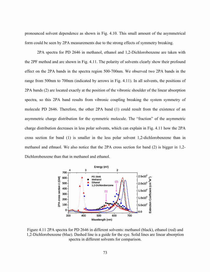
pronounced solvent dependence as shown in Fig. 4.10. This small amount of the asymmetrical

form could be seen by 2PA measurements due to the strong effects of symmetry breaking.

2PA spectra for PD 2646 in methanol, ethanol and 1,2-Dichlorobenzene are taken with

the 2PF method and are shown in Fig. 4.11. The polarity of solvents clearly show their profound

effect on the 2PA bands in the spectra region 500-700nm. We observed two 2PA bands in the

range from 500nm to 700nm (indicated by arrows in Fig. 4.11). In all solvents, the positions of

2PA bands (2) are located exactly at the position of the vibronic shoulder of the linear absorption

spectra, so this 2PA band results from vibronic coupling breaking the system symmetry of

molecule PD 2646. Therefore, the other 2PA band (1) could result from the existence of an

asymmetric charge distribution for the symmetric molecule. The “fraction” of the asymmetric

charge distribution decreases in less polar solvents, which can explain in Fig. 4.11 how the 2PA

cross section for band (1) is smaller in the less polar solvent 1,2-dichlorobenzene than in

methanol and ethnaol. We also notice that the 2PA cross section for band (2) is bigger in 1,2-

Dichlorobenzene than that in methanol and ethanol.

(1)

(2)

300 400 500 600 700

0

100

200

300

400

500

600

700

2PA

cro

ss s

ectio

n δ

(GM

)

Wavelength (nm)

PD 2646 Methanol Ethanol 1,2-Dichlorobenzene

0.0

5.0x104

1.0x105

1.5x105

2.0x105

2.5x105

Extin

ctio

n C

oeffi

cien

t (cm

-1M

-1)

4 3 2Energy (eV)

(1)

(2)

300 400 500 600 700

0

100

200

300

400

500

600

700

2PA

cro

ss s

ectio

n δ

(GM

)

Wavelength (nm)

PD 2646 Methanol Ethanol 1,2-Dichlorobenzene

0.0

5.0x104

1.0x105

1.5x105

2.0x105

2.5x105

Extin

ctio

n C

oeffi

cien

t (cm

-1M

-1)

4 3 2Energy (eV)

Figure 4.11 2PA spectra for PD 2646 in different solvents: methanol (black), ethanol (red) and 1,2-Dichlorobenzene (blue). Dashed line is a guide for the eye. Solid lines are linear absorption

spectra in different solvents for comparison.

73

2PA spectra for asymmetric PD 2755 in methanol, ethanol and 1,2-Dichlorobenzene are

taken with the 2PF method and are shown in Fig. 4.12. Two arrows indicate that there are two

2PA bands for PD 2755 in ethanol. We also can see the similar two 2PA bands for PD 2755 in

Dichlorobenzene. Band (1) is located at the position of the vibronic shoulder of the linear

absorption spectrum due to vibrational coupling. Band (2) corresponds to the linear absorption

peak. Because PD 2755 is an asymmetric molecule, 2PA into the first excited state S1 is allowed.

We can also consider band (2) is due to the asymmetric charge distribution of PD 2755, so the

2PA cross section of band (2) is smaller in the less polar solvent 1,2-dichlorobenzene than it is in

ethanol, as experimentally observed.

300 400 500 600 700

0

100

200

300

400

500

600

700

800 PD 2755

Ethanol Dichlorobenzene

2PA

cro

ss s

ectio

n δ

(GM

)

Wavelength (nm)

0.0

0.2

0.4

0.6

0.8

1.0

1.2

Nor

mal

ized

1P

A

4 3.5 3 2.5 2Energy (eV)

(1)

(2)

300 400 500 600 700

0

100

200

300

400

500

600

700

800 PD 2755

Ethanol Dichlorobenzene

2PA

cro

ss s

ectio

n δ

(GM

)

Wavelength (nm)

0.0

0.2

0.4

0.6

0.8

1.0

1.2

Nor

mal

ized

1P

A

4 3.5 3 2.5 2Energy (eV)

(1)

(2)

Figure 4.12 2PA spectra for PD 2755 in different solvents: ethanol (blue) and 1,2-dichlorobenzene (red). Dashed line is for a guide for the eye. Solid lines are linear absorption

spectra in different solvents for comparison.

These experimental studies are just preliminary results for investigating the nature of the

weak 2PA band and symmetry breaking for symmetric molecules. More experiments and

detailed quantum chemical calculations are needed to fully understand this nature.

74

4.7 Effect of bridge

We studied the effect of placing bridge molecules in the middle of conjugated chains on

the 2PA properties by comparing PD 2646 with PD 200, as well as PD 3428 with PD 2093.

Molecular structures are shown in Fig. 4.13 (a) and Fig. 4.14 (a). Degenerate 2PA spectra of

these molecules in the solvent ethanol were taken by using 2PF spectroscopy and Z-scan. 2PA

spectra as well as linear absorption spectra with extinction coefficients are shown in Fig. 4.13 (b)

and Fig. 4.14 (b). Here the 2PA cross-section δ is plotted versus the half of input photon

wavelengths.

PD 2646 PD 200

S

NCH3

S

NCH3

CH3C6H4SO3

+

-

S

NC2H5

S

NC2H5

CH3C6H4SO3

+

-

PD 2646 PD 200

S

NCH3

S

NCH3

CH3C6H4SO3

+

-

S

NC2H5

S

NC2H5

CH3C6H4SO3

+

-

(a)

300 400 500 600 700 800

0

100

200

300

400

500

600

700

800

2PA

cros

s se

ctio

n δ

(GM

)

Wavelength (nm)

PD2646 PD200

0.0

5.0x104

1.0x105

1.5x105

2.0x105

2.5x105

Extin

ctio

n C

oeffi

cien

t (cm

-1M

-1)

4 3 2Energy (eV)

(b)

Figure 4.13 (a) molecular structures; (b) degenerate 2PA spectra for PD200, PD2646, dashed line is for theoretical fitting based on Eq. (2.55), and linear absorption spectra (solid line) are shown

for reference.

75

Introduction of the bridges (or partial cyclization of the chain) with the goal of increasing

the photochemical stability, depending on the position of cyclization, leads to blue shifts

(compare PD 2646 with PD 200) or red shifts (compare PD 3428 with PD 2093) of the linear

absorption peaks relative to the unbridged chromophores.

PD 3428 PD 2093

NN

CH3 CH3

CH3CH3

+

ClO4-

C6H5

N

CH3CH3

N

CH3CH3

ClO4

+

-

PD 3428 PD 2093

NN

CH3 CH3

CH3CH3

+

ClO4-

C6H5

N

CH3CH3

N

CH3CH3

ClO4

+

-

(a)

300 400 500 600 700 800 9000

500

1000

1500

2000

2500

2PA

cros

s se

ctio

n δ

(GM

)

Wavelength (nm)

PD3428 PD2093

0.0

5.0x104

1.0x105

1.5x105

2.0x105

2.5x105

3.0x105

Ext

inct

ion

Coe

ffici

ent (

cm-1M

-1)

4 3.5 3 2.5 2 1.5Energy (eV)

(b)

Figure 4.14 (a) molecular structures; (b) degenerate 2PA spectra for PD3428, PD2093, dashed line is for theoretical fitting based on Eq. (2.55), and linear absorption spectra (solid line) are

shown for reference.

We note that the bridged structures (PD 200, PD 2093) are characterized by smaller

values of 2PA cross section δ in the first 2PA band. From Section 4.6, this weak 2PA band is due

to symmetry breaking of symmetric molecules. So it is reasonable to consider that the

76

introduction of the bridges can protect the symmetric molecular structure from this symmetry

breaking, thus the smaller 2PA cross section δ.

77

CHAPTER 5 STRUCTURE-PROPERTY OF SQUARAINE, CROCONIUM AND TETRAON

5.1 Squaraine dyes

Squaraine dyes (SDs) also belong to the family of cyanines. SDs insert an electron

acceptor C4O2 fragment at the center of the chromophore chain, which can be chemically

considered as a simultaneous cyclization of the polymethine chain by the C=O bridge shown in

Fig.5.1 (a). Introduction of the anionic substitute O - to the central position of the polymethine

molecule makes the squaraine molecule formally neutral, or more correctly, it can be considered

as a bi-ionic molecule with separated positive and negative charges. By placing terminal groups

R1 and R2, we studied SDs with different structures shown in Fig.5.1 (b), which are synthesized

at the Institute of Organic Chemistry, National Academy of Science, Kiev, Ukraine by standard

methods as described in Ref. [64]. There are other SDs shown in Fig.5.11 in Section 5.4, which

are synthesized by Dr. Seth Marder’s group at the School of Chemistry and Biochemistry and

Center for Organic Photonics and Electronics, Georgia Institute of Technology, Atlanta.

Similar to polymethine dyes (PDs), Squaraine dyes are also attractive for 2PA due to

three advantages: 1) they show large ground-state transition dipole moments; 2) they have close

to parallel orientation of their ground- and excited-state transition dipole moments; 3) their even

sharper (than for PDs) low-energy side of the linear absorption spectra allows significant

intermediate state resonance enhancement of the 2PA. The comparison of 2PA property between

SDs and PDs will be discussed in Section 5.2

78

O

O

NR2

R1N

+-

(a)

N

O

OH O

N

OH CH3

CH3

CH3

CH3

+

SD 1408

NO

OCH3CH3

CH3CH3

NC3H7

C3H7

+

SD 2577

Nn-C4H9

CH3CH3 O

O

N

CH3CH3

n-C4H9

+

SD 2243

N

O

OH O

N

OH CH3

CH3

CH3

CH3

+

SD 1408

NO

OCH3CH3

CH3CH3

NC3H7

C3H7

+

SD 2577

Nn-C4H9

CH3CH3 O

O

N

CH3CH3

n-C4H9

+

SD 2243

(b)

Figure 5.1 Squaraine dyes (SDs): (a) electron acceptor C4O2 fragment at the center of the chain, R1 and R2 are terminal groups; (b) SDs synthesized in Institute of Organic Chemistry, National

Academy of Sciences, Ukraine

5.2 Comparison between polymethines and squaraines

We performed experimental and theoretical studies for two polymethine dyes (PDs) and

two squaraine dyes (SDs) with analogous structures to study the effects of the squaraine on the

2PA properties and provide a deeper insight into the nature of 2PA processes.

The molecular structures are shown in Fig. 5.2 (a) and Fig. 5.3 (a). SD 2577 and PD 2350

have the same indolium terminal groups and similar conjugation lengths. SD 2243 and PD 2630

also have the same benzoindolium terminal groups and similar conjugation lengths. Linear

absorption and fluorescence spectra are shown in Fig. 5.2 (b) and 5.3 (b). Experimental data

show that SDs have narrower linear absorption bands than PDs allowing a smaller detuning

energy, ∆E, to be accessed for 2PA, leading to a larger intermediate state resonance enhancement,

and thus a larger 2PA cross section. SDs typically are characterized by narrower absorption

79

bands because of the smaller change in bond lengths when excited by a photon. The Central

acceptor group leads to a less pronounced bond alternation as compared to PDs. Therefore their

Frank-Condon potential curves (ground and excited) are less shifted with respect to each other.

Degenerate 2PA spectra of these molecules were also taken by using 2PF spectroscopy

and Z-scan. 2PA spectra as well as linear absorption spectra with extinction coefficients are

shown in Fig. 5.2 (c) and 5.3 (c). The 2PA cross section δ is plotted versus the half of input

photon wavelengths. A summary of ground state transition dipole moments µ01, calculated

excited state transition dipole moments µ12, maximum 2PA cross section δmax, as well as

detuning energy ∆E are shown in Table 5.1 and Table 5.2. PD 2350, SD 2577 and PD 2630 are

measured in ethanol, but SD 2243 is measured in CH2CL2 due to poor solubility in ethanol.

Table 5.1 Parameters for polymethine and squaraine with analogous structures: PD2350 and SD2577 in ethanol

Molecules µ01(debye) µ12(debye) δmax1 δmax2 δmax3 ∆E*

PD2350 14.7 2.8 130 GM 710 GM N/A 0.31eV SD2577 12.2 4.2 36 GM 740 GM 5000 GM 0.21eV

* Detuning energy ∆E for PD 2350 is calculated for 2PA peak δmax2, and ∆E for SD2577 is calculated for 2PA peak δmax3

Table 5.2 Parameters for polymethine and squaraine with analogous structures: PD2630 and SD2243

Molecules µ01(Debye) µ12(Debye) δmax1 δmax2 δmax3 ∆E PD2630 14 3.1 140 GM 980 GM > 1200 GM 0.21 eV SD2243 13.8 3.5 80 GM 1000 GM >7000 GM 0.2 eV

80

PD2350 SD2577

NO

OCH3CH3

CH3CH3

NC3H7

C3H7

+N

CH3

CH3

C3H7

NC3H7

CH3

CH3

I

+

PD2350 SD2577

NO

OCH3CH3

CH3CH3

NC3H7

C3H7

+N

CH3

CH3

C3H7

NC3H7

CH3

CH3

I

+

(a)

300 400 500 600 700

0.0

0.2

0.4

0.6

0.8

1.0

Line

ar a

bsor

ptio

n (a

.u.)

Wavelength (nm)

PD2350 SD2577

4 3.5 3 2.5 2

Energy (eV)

550 600 650 700 750 800

0.0

0.2

0.4

0.6

0.8

1.0

Fluo

resc

ence

(a.u

.)

Wavelength (nm)

PD2350 SD2577

2.2 2 1.8 1.6

Energy (eV)

(b)

300 400 500 600 700

0

1000

2000

3000

4000

5000

2PA

cro

ss s

ectio

n δ

(GM

)

Wavelength (nm)

PD2350 SD2577

0.0

5.0x104

1.0x105

1.5x105

2.0x105

2.5x105

3.0x105

3.5x105

Ext

inct

ion

Coe

ffici

ent (

cm-1 M

-1)

4 3.5 3 2.5 2Energy (eV)

(c)

Figure 5.2 (a) Molecular structure of PD2350 and SD2577; (b) Linear absorption and fluorescence spectra in ethanol; (c) 2PA spectra in ethanol (dotted, dashed line for theoretical

fitting) and linear absorption spectra (solid lines) shown as extinction coefficient

81

PD2630 SD2243

Nn-C4H9

CH3CH3 O

O

N

CH3CH3

n-C4H9

+N

CH3CH3

N

CH3 CH3

C2H5 C2H5

p-CH3C6H4SO3

+

-

PD2630 SD2243

Nn-C4H9

CH3CH3 O

O

N

CH3CH3

n-C4H9

+N

CH3CH3

N

CH3 CH3

C2H5 C2H5

p-CH3C6H4SO3

+

-

(a)

400 500 600 700 800

0.0

0.2

0.4

0.6

0.8

1.0

Line

ar a

bsor

ptio

n (a

.u.)

Wavelength (nm)

PD 2630 SD 2243

3.5 3 2.5 2Energy (eV)

600 700 800 900 1000

0.0

0.2

0.4

0.6

0.8

1.0

Flur

esce

nce

(a.u

.)

Wavelength (nm)

PD 2630 SD 2243

2.2 2 1.8 1.6 1.4 1.2

Energy (eV)

(b)

300 400 500 600 700 800

0

2000

4000

6000

8000

10000

2PA

cros

s se

ctio

n δ

(GM

)

Wavelength (nm)

PD2630 SD2243

0

1x105

2x105

3x105

4x105

Extin

ctio

n C

oeffi

cien

t (cm

-1M

-1)

4 3.5 3 2.5 2Energy (eV)

(c)

Figure 5.3 (a) Molecular structure of PD2630 and SD2243; (b) Linear absorption and fluorescence spectra; (c) 2PA spectra (doted, dashed line for theoretical fitting) and linear

absorption spectra shown as extinction coefficient. PD 2630 in ethanol and SD 2243 in CH2CL2

82

1) Weakly allowed 2PA band:

Our measurements show the existence of a weakly allowed 2PA band within the vibronic

shoulder of the first absorption band, S0 → S1, for which the transition is forbidden by dipole

selection rules for these symmetrical molecules. It is commonly accepted that two-photon

excitation to S1 involves two dipole moments: µ01 and ∆µ (vector difference between permanent

S0 and S1 dipoles). According to the traditional quantum-chemical theories [59], for symmetrical

polymethine dyes (symmetry C2v) ∆µ is oriented perpendicular to µ01 and for the symmetrical

squarylium dyes (symmetry C2i) ∆µ = 0 which would both prohibit 2PA to the S1 state.

Cross sections for these weak 2PA bands are: 140 GM for PD 2350 (peak position at ≈

590 nm); 40 GM for SD 2577 (peak position at ≈ 570 nm); 160 GM for PD 2630 (peak position

at ≈ 625 nm), and 85 GM for SD 2243 (peak position at ≈ 625 nm). We note that cross sections

for squaraine dyes are smaller than for polymethines, which may be connected with the different

molecular symmetry. As was already mentioned, symmetrical polymethine dyes have C2v

symmetry and a non-zero ∆µ value. As a result, this band is slightly allowed by dipole selection

rules in contrast to being a forbidden band in the centrosymmetrical SDs with ∆µ = 0.

2) Main 2PA bands:

Considering the more intense 2PA bands, for PD 2350 shown in Fig. 5.2 (c), our

measurements reveal the position of the second 2PA band at ∼ 390 nm (~780nm excitation) with

δ2PA ≈ 720 GM. Further tuning of the excitation wavelength into the shorter wavelength region is

impossible due to the presence of one-photon absorption from the S0 → S1 band.

Fig. 5.2 (c) shows the analogous information for SD 2577. In contrast to PD 2350, the

2PA spectrum for SD 2577 includes three bands: a weakly allowed band at the vibronic shoulder

83

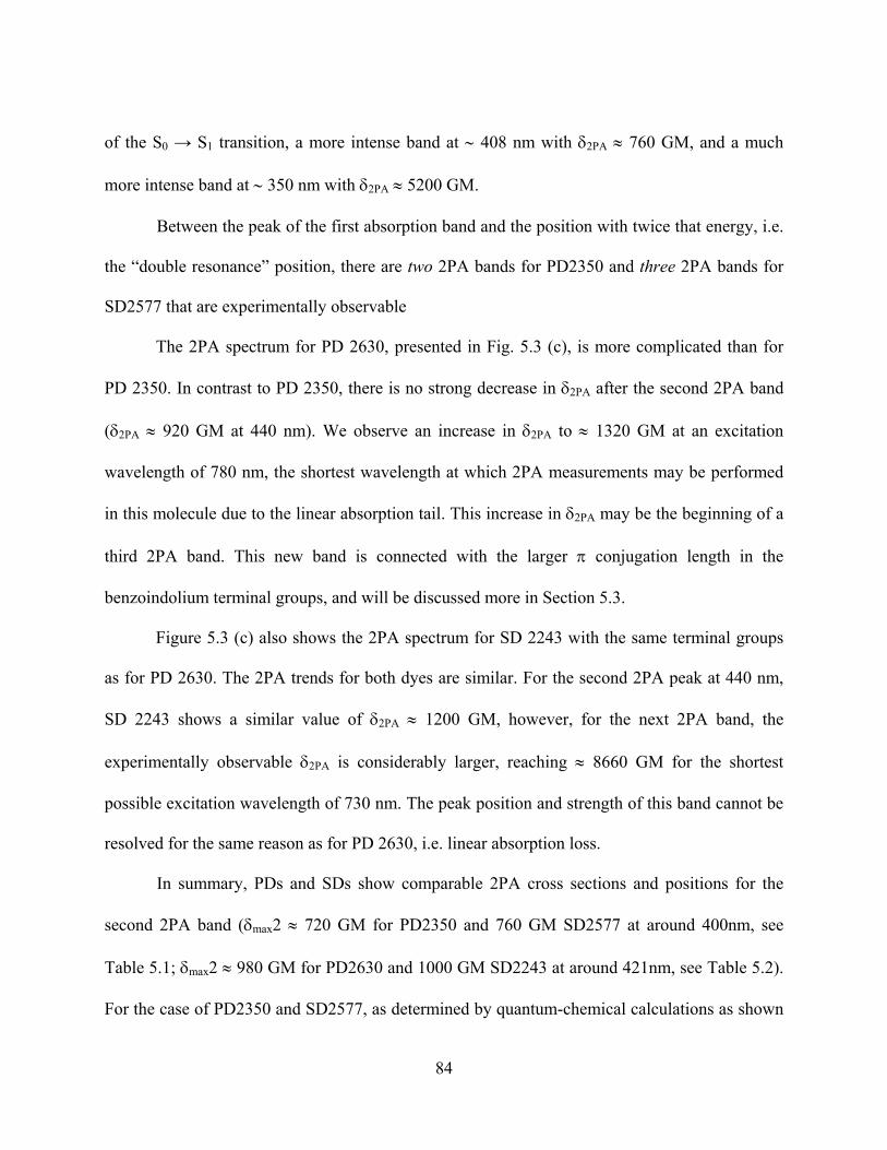
of the S0 → S1 transition, a more intense band at ∼ 408 nm with δ2PA ≈ 760 GM, and a much

more intense band at ∼ 350 nm with δ2PA ≈ 5200 GM.

Between the peak of the first absorption band and the position with twice that energy, i.e.

the “double resonance” position, there are two 2PA bands for PD2350 and three 2PA bands for

SD2577 that are experimentally observable

The 2PA spectrum for PD 2630, presented in Fig. 5.3 (c), is more complicated than for

PD 2350. In contrast to PD 2350, there is no strong decrease in δ2PA after the second 2PA band

(δ2PA ≈ 920 GM at 440 nm). We observe an increase in δ2PA to ≈ 1320 GM at an excitation

wavelength of 780 nm, the shortest wavelength at which 2PA measurements may be performed

in this molecule due to the linear absorption tail. This increase in δ2PA may be the beginning of a

third 2PA band. This new band is connected with the larger π conjugation length in the

benzoindolium terminal groups, and will be discussed more in Section 5.3.

Figure 5.3 (c) also shows the 2PA spectrum for SD 2243 with the same terminal groups

as for PD 2630. The 2PA trends for both dyes are similar. For the second 2PA peak at 440 nm,

SD 2243 shows a similar value of δ2PA ≈ 1200 GM, however, for the next 2PA band, the

experimentally observable δ2PA is considerably larger, reaching ≈ 8660 GM for the shortest

possible excitation wavelength of 730 nm. The peak position and strength of this band cannot be

resolved for the same reason as for PD 2630, i.e. linear absorption loss.

In summary, PDs and SDs show comparable 2PA cross sections and positions for the

second 2PA band (δmax2 ≈ 720 GM for PD2350 and 760 GM SD2577 at around 400nm, see

Table 5.1; δmax2 ≈ 980 GM for PD2630 and 1000 GM SD2243 at around 421nm, see Table 5.2).

For the case of PD2350 and SD2577, as determined by quantum-chemical calculations as shown

84

in Section 5.3, introduction of the donor indolium terminal groups to the unsubstituted

polymethine chain increases the density of the occupied molecular orbitals, and thus the number

of electronic transitions between the first band S0 → S1, and the position of twice the energy of

the first band. Relatively high δ2PA ≈ 700 GM can be observed due to a strong coupling of initial

and final molecular orbitals via the intermediate level.

Quantum-chemical calculations (see Section 5.3) show another way to increase the

number of active two-photon transitions by increasing the density of unoccupied molecular

orbitals. This was achieved by introducing acceptor fragments to the squaraine molecules. The

distinguishing feature of SD2577 is the possibility to access the third and most intense 2PA band.

This higher lying third 2PA band (δmax3 ≈ 5200 GM for SD2577) displays a much larger δ due to

a decrease in the detuning energy ∆E leading to a large enhancement of cross section values, i.e.

significant resonance enhancement of the 2PA cross section for both the intermediate and final

states.. This peak is observable just below the linear absorption edge.

5.3 Quantum-chemical calculations and analysis

5.3.1 Methodology of quantum-chemical calculations

Quantum-chemical calculations are performed by Dr. Olga V. Przhonska and her

colleagues at Institute of Organic Chemistry, National Academy of Sciences, Ukraine. Quantum-

chemical calculations were performed with the goal of understanding the spectral position of

2PA bands and revealing the origin of the high 2PA cross section δ2PA in squaraine molecules.

Quantum-chemical calculations were carried out at the Institute of Organic Chemisty, National

Academy of Sciences, Ukraine. For the calculations of the positions of the electronic levels and

85

the shapes of the molecular orbitals, a well-known MOLCAO (Molecular Orbital as a Linear

Combination of Atomic Orbitals) method was used [59]. The wavefunction of the i-th molecular

orbital (MO) iϕ was written as an expansion of the atomic orbitals µχ :

(5.1) ∑=µ

µµ χϕ ii C

where are the corresponding coefficients, and the summation runs over all the atomic

orbitals. We note that is the probability of the location of an electron in the i-th MO in the

neighborhood of the µ-th atom [59]. Calculations were performed in the framework of the

standard semi-empirical approximations (HyperChem package). The equilibrium molecular

geometries were calculated employing the Austin Model 1 (AM1) method with the energy

change step, i.e. gradient, 0.01 kcal/mol. It was established previously that the lengths of the

carbon-carbon bonds calculated in this method are in good agreement with the corresponding

values obtained by an ab initio approximation [65].

µiC

2µiC

The π-system of all molecules was found to be planar. Characteristics of the electron

transitions were obtained in the ZINDO/S approximation with spectral parameterization. The

wavefunction of the p-th excited state Ψp was built as an expansion of the electronic

configurations corresponding to electron transfer from the occupied i-th to vacant j-th

orbital:

ji→Φ

∑ →→ Φ=ji

jijipp T,

,ψ (5.2)

where are the normalized coefficients, and indices i and j run over all MOs.

is a normalization condition. In our calculations we used all π → π* single excited

jipT →, 1,

2, =∑ →

jijipT

86

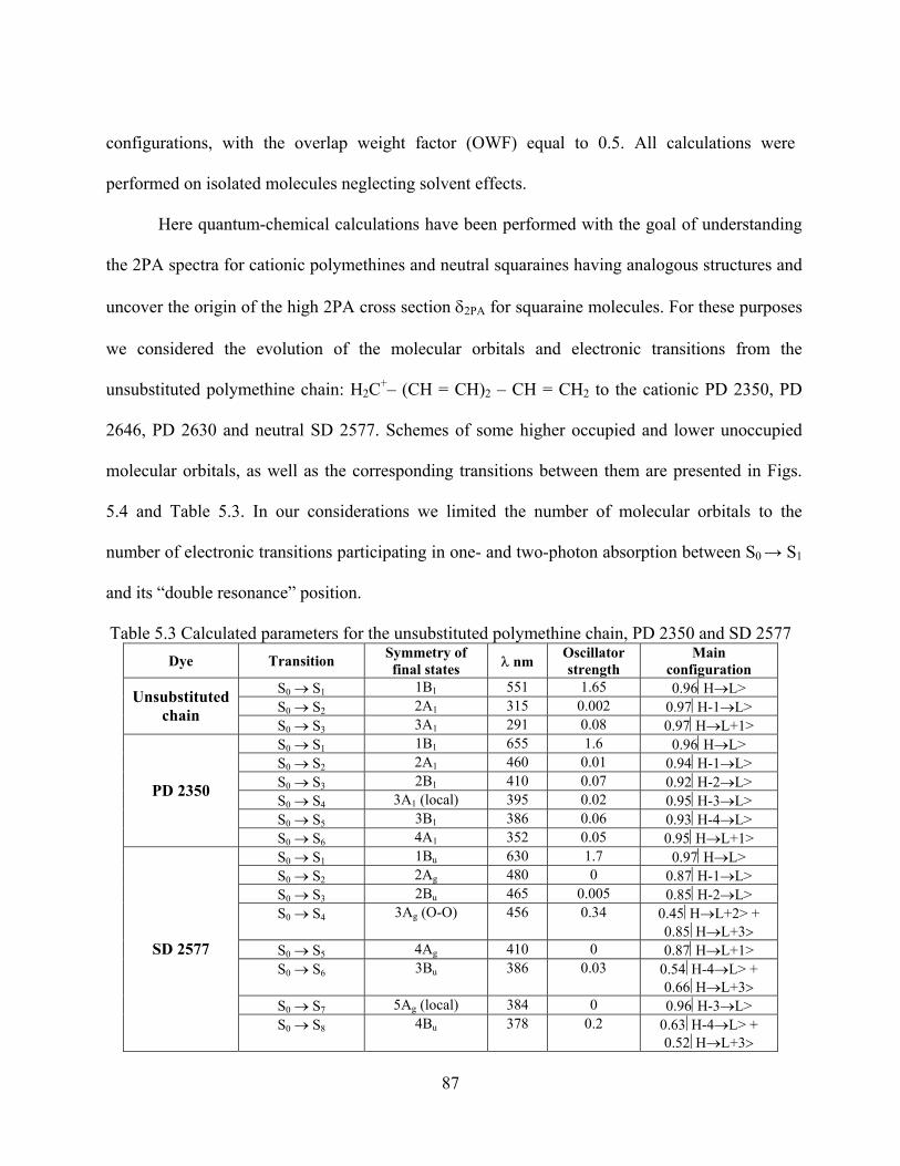
configurations, with the overlap weight factor (OWF) equal to 0.5. All calculations were

performed on isolated molecules neglecting solvent effects.

Here quantum-chemical calculations have been performed with the goal of understanding

the 2PA spectra for cationic polymethines and neutral squaraines having analogous structures and

uncover the origin of the high 2PA cross section δ2PA for squaraine molecules. For these purposes

we considered the evolution of the molecular orbitals and electronic transitions from the

unsubstituted polymethine chain: H2C+– (CH = CH)2 – CH = CH2 to the cationic PD 2350, PD

2646, PD 2630 and neutral SD 2577. Schemes of some higher occupied and lower unoccupied

molecular orbitals, as well as the corresponding transitions between them are presented in Figs.

5.4 and Table 5.3. In our considerations we limited the number of molecular orbitals to the

number of electronic transitions participating in one- and two-photon absorption between S0 → S1

and its “double resonance” position.

Table 5.3 Calculated parameters for the unsubstituted polymethine chain, PD 2350 and SD 2577 Dye Transition Symmetry of

final states λ nm Oscillator strength

Main configuration

S0 → S1 1B1 551 1.65 0.96⎢H→L> S0 → S2 2A1 315 0.002 0.97⎢H-1→L>

Unsubstituted chain

S0 → S3 3A1 291 0.08 0.97⎢H→L+1> S0 → S1 1B1 655 1.6 0.96⎢H→L> S0 → S2 2A1 460 0.01 0.94⎢H-1→L> S0 → S3 2B1 410 0.07 0.92⎢H-2→L> S0 → S4 3A1 (local) 395 0.02 0.95⎢H-3→L> S0 → S5 3B1 386 0.06 0.93⎢H-4→L>

PD 2350

S0 → S6 4A1 352 0.05 0.95⎢H→L+1> S0 → S1 1Bu 630 1.7 0.97⎢H→L> S0 → S2 2Ag 480 0 0.87⎢H-1→L> S0 → S3 2Bu 465 0.005 0.85⎢H-2→L> S0 → S4 3Ag (O-O) 456 0.34 0.45⎜H→L+2> +

0.85⎜H→L+3> S0 → S5 4Ag 410 0 0.87⎢H→L+1> S0 → S6 3Bu 386 0.03 0.54⎜H-4→L> +

0.66⎜H→L+3> S0 → S7 5Ag (local) 384 0 0.96⎢H-3→L>

SD 2577

S0 → S8 4Bu 378 0.2 0.63⎜H-4→L> + 0.52⎜H→L+3>

87

1Bu

1Ag

2Ag

3Ag

4Ag

5Ag

2Bu

3Bu

4Bu

S0

S2

S1

S4

S5

S6

S7

S8

S32A1

3A1

4A1

2B1

3B1

1A1

1B1S1

S2

S3

S4

S5

S6

S01A1

2A1

3A1

1B1

S0

S1

S2

S3

Chain PD2350 SD2577

1Bu

1Ag

2Ag

3Ag

4Ag

5Ag

2Bu

3Bu

4Bu

S0

S2

S1

S4

S5

S6

S7

S8

S3

1Bu

1Ag

2Ag

3Ag

4Ag

5Ag

2Bu

3Bu

4Bu

S0

S2

S1

S4

S5

S6

S7

S8

S32A1

3A1

4A1

2B1

3B1

1A1

1B1S1

S2

S3

S4

S5

S6

S01A1

2A1

3A1

1B1

S0

S1

S2

S3

1A1

2A1

3A1

1B1

S0

S1

S2

S3

Chain PD2350 SD2577

Figure 5.4 Scheme of the electronic transitions for the unsubstituted chain, PD 2350 and SD 2577. Dashed lines indicate one-photon allowed transitions; solid lines indicate allowed two-photon transitions; bold solid lines indicate experimentally observed two-photon transitions.

5.3.2 Unsubstituted polymethine chain

Quantum-chemical calculations of the unsubstituted polymethine chain show in Fig.5.4 –

Fig. 5.6 that the ground to first excited state transition S0 → S1 is allowed by symmetry rules

(1A1 → 1B1) and is connected with the electron transfer between the highest occupied molecular

orbital (HOMO) and the lowest unoccupied molecular orbital (LUMO). The two next electronic

88

transitions, S0 → S2 (1A1 → 2A1) and S0 → S3 (1A1→ 3A1), are forbidden and correspond to

HOMO-1 → LUMO and HOMO → LUMO+1 respectively (see Table 5.3).

These transition energies are close but not exactly equal to each other. The calculated

spectral shift between the corresponding S0 → S2 and S0 → S3 absorption bands is ≈ 20 nm, i.e.

no degeneracy. This is the origin of the main difference between the spectra of the cationic

polymethine chain and its neutral polyene analogue. The polyene chain is characterized by the

formation of double (for Au → Au) and triple (for Bg → Bg) degenerate configurations leading to

energy level splitting and to a redistribution of oscillator strengths [22]. This makes the least

energetic transition disallowed for 1PA but allowed for 2PA.

For the polymethine chain, one of the A1 → A1 transitions approximately corresponds to

a “double resonance” position of the main absorption band, which makes it impossible to reach

this 2PA peak experimentally, again due to linear absorption. We emphasize that all molecular

orbitals in the unsubstituted conjugated polymethine chain are totally and uniformly delocalized,

and all electronic transitions are described mainly by single configurations with coefficients

Tp,i→j > 0.9 (see Table 5.3).

89

LUMO+1

HOMO-1

LUMO

HOMO

Unsubstituted Chain

LUMO+1

HOMO-1

LUMO

HOMO

Unsubstituted Chain

LUMO

HOMO

HOMO-1

Terminal Group

LUMO

HOMO

HOMO-1

LUMO

HOMO

HOMO-1

Terminal Group

Figure 5.5 Electron density distribution in the molecular orbitals for the unsubstituted polymethine chain and indolium terminal groups.

90

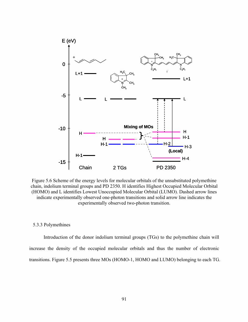
0

-5

-10

-15

E (eV)

H-1

L

HH

L

L+1

H-1

+

N

CH3

CH3

CH3

CH3

+

Chain 2 TGs

HH-1

H-2H-3

H-4

L

L+1

(Local)

PD 2350

N

CH3

CH3

C3H7

NC3H7

CH3

CH3

I

+

Mixing of MOs

0

-5

-10

-15

E (eV)

0

-5

-10

-15

E (eV)

H-1

L

HH-1

L

HH

L

L+1

H-1

H

L

L+1

H-1

+

N

CH3

CH3

CH3

CH3

+

Chain 2 TGs

HH-1

H-2H-3

H-4

L

L+1

(Local)

PD 2350

N

CH3

CH3

C3H7

NC3H7

CH3

CH3

I

+

Mixing of MOs

Figure 5.6 Scheme of the energy levels for molecular orbitals of the unsubstituted polymethine chain, indolium terminal groups and PD 2350. H identifies Highest Occupied Molecular Orbital (HOMO) and L identifies Lowest Unoccupied Molecular Orbital (LUMO). Dashed arrow lines

indicate experimentally observed one-photon transitions and solid arrow line indicates the experimentally observed two-photon transition.

5.3.3 Polymethines

Introduction of the donor indolium terminal groups (TGs) to the polymethine chain will

increase the density of the occupied molecular orbitals and thus the number of electronic

transitions. Figure 5.5 presents three MOs (HOMO-1, HOMO and LUMO) belonging to each TG.

91

LUMO

HOMO

HOMO-2

HOMO-3

HOMO-4

LUMO+1

HOMO-2

HOMO-1

Figure 5.7 Electron density distribution in the molecular orbitals for PD 2350

92

As shown in Fig. 5.6 and Fig. 5.7, two HOMO orbitals of both TGs are completely mixed

with the HOMO of the unsubstituted polymethine chain producing three delocalized molecular

orbitals HOMO, HOMO-1 and HOMO-4. In symmetrical PDs such as PD 2350, there are two

identical HOMO-1s of TGs (with charge localization only at TGs see in Fig. 5.5). This is an

origin of the energy splitting. The splitting energy depends on the TG’s donor properties. After

splitting, one of these MOs typically mixes with the orbital of the chain producing a delocalized

molecule orbital, HOMO-2, shown in Fig. 5.6 and Fig. 5.7, and the other MO remains localized at

the TGs (see HOMO-3 shown in Fig. 5.6 and Fig. 5.7). Thus, the interaction of the MOs of all the

molecular fragments (mixing among HOMOs from chain and two TGs) in PD 2350 leads to

delocalization of the three highest occupied MOs of PD 2350 (HOMO, HOMO-1, HOMO-2

shown in Fig. 5.6). This occurs not only along the polymethine chain, but also extends through the

TGs. Therefore, introduction of the indolium TGs with their own conjugated systems causes a

considerable effective lengthening of the chromophore.

Note that LUMO and LUMO+1 extend the chain conjugation to the nitrogen atoms of

both TGs, while the π-electron conjugations at HOMO, HOMO-1 and HOMO-2 spread out over

the entire molecule. In total, 7 molecular orbitals (from HOMO-4 to LUMO+1), shown in Fig. 5.7,

are necessary for the quantum-chemical analysis.

It is commonly accepted that the electron transfer between the HOMO and LUMO (S0 →

S1, 1A1→ 1B1 transition) corresponds to the intense long wavelength band in the one-photon

absorption spectrum. The next transition involving practically pure HOMO-1 and LUMO (see

coefficients Tp,i→j in the Table 5.3) and being of the 1A1→ 2A1 symmetry, should correspond to

the lowest two-photon transition. However, based on the results of the quantum-chemical

calculations, we suggest that only the next 1A1→ 3A1 (S0 → S4) transition in Fig. 5.4 for PD2350,

93

corresponding to the electron transfer between the localized HOMO-3 and delocalized LUMO is

the most active in 2PA for PD 2350. This is in agreement with the experimental spectral position

of the second 2PA band seen in Fig. 5.2 at ∼ 390 nm.

The existence of this local molecular orbital is of great importance for the 2PA. The

transition from HOMO-3 to LUMO (1A1→ 1A3, S0 → S4 in Table 5.3) gives zero overlap (see in

Fig.5.7), thus it requires an intermediate (HOMO) state and forms a two-photon absorbing

transition. Our understanding is that the localized – delocalized electron transition, such as

HOMO-3 → LUMO, which appears in the energy interval between the S0 → S1 and its “double

resonance”, is responsible for the strong 2PA band with peak at 390nm.

The main characteristic feature of the 2PA spectrum for the PDs is the relatively high 2PA

cross section δ2PA of ≈ 600 – 1000 GM (for dicarbocyanines with different TGs, see the Section

4.4) due to the strong coupling of these orbitals with the intermediate HOMO, see Fig. 5.7.

94

0

-5

-10

-15

E (eV)

PD 2350

N

CH3

CH3

C3H7

NC3H7

CH3

CH3

I

+

PD 2630

N

CH3CH3

N

CH3 CH3

C2H5 C2H5

p-CH3C6H4SO3

+

-

H-2

HH-1

H-3

H-4

L

L+1

(Local)

HH-1

H-2 H-3

H-4

L

L+1

(Local)

PD 2646

H-2

HH-1

H-3

H-4

L

L+1

(Local)

S

N+

S

N

CH3CH3

CH3C6H4SO3-

0

-5

-10

-15

E (eV)

0

-5

-10

-15

E (eV)

PD 2350

N

CH3

CH3

C3H7

NC3H7

CH3

CH3

I

+

PD 2630

N

CH3CH3

N

CH3 CH3

C2H5 C2H5

p-CH3C6H4SO3

+

-

H-2

HH-1

H-3

H-4

L

L+1

(Local)H-2

HH-1

H-3

H-4

L

L+1

(Local)

HH-1

H-2 H-3

H-4

L

L+1

(Local)

HH-1

H-2 H-3

H-4

L

L+1

(Local)

PD 2646

H-2

HH-1

H-3

H-4

L

L+1

(Local)H-2

HH-1

H-3

H-4

L

L+1

(Local)

S

N+

S

N

CH3CH3

CH3C6H4SO3-

Figure 5.8 Scheme of the energy levels for molecular orbitals of PD 2646, PD 2350 and PD 2630. H identifies the Highest Occupied Molecular Orbital (HOMO) and L identifies the Lowest Unoccupied Molecular Orbital (LUMO). Dashed arrow lines indicate experimentally observed

one-photon transitions and solid arrow lines indicate experimentally observed two-photon transitions.

In order to further increase the density of occupied molecular orbitals and thus the number

of electronic transitions, we choose TGs with more extended π-systems. This idea was realized in

PD 2630 containing more complicated benzoindolium terminal groups (see Section 4.4 and Fig.

5.8). As compared to PD 2350, this dye is characterized by red-shifted absorption bands. Note

that experimentally the main one-photon absorption peak is shifted by ≈ 0.1 eV, and the 2PA band

95

is shifted more to the red by ≈ 0.18 eV. Due to this shift, the beginning of the next, third 2PA

band (corresponding to transition HOMO L+1 in Fig. 5.8, 1A1 4A1 and S0 S6 in Fig.

5.4), has been experimentally measured (see Fig. 4.5(b)). Analyzing the evolution of the 2PA

bands from the unsubstituted chain to PD 2350, and then to PD 2630, we assume that the spectral

shift of the 2PA peak is primarily due to the terminal groups. More extended TGs may provide an

additional shift increasing the number of experimentally reachable 2PA bands.

5.3.4 Squaraines

An alternative way to increase the number of active two-photon transitions, 1A1→ mA1,

can be provided by an increase of the density of unoccupied molecular orbitals. This has been

achieved in the dyes of another type – squaraines. Inserting the high acceptor C4O2 fragment in

the center of the polymethine chain, while keeping the same TG, can be chemically considered as

a simultaneous cyclization of the chain by the C=O bridge and introduction of the anionic

substituents O- to the central position of the PD 2350 (or PD 2630). The latter makes the SD-

molecule formally neutral, or more correctly, it can be considered as a bi-ionic molecule with

separated positive and negative charges.

In the case of SD 2577, five HOMO’s and five LUMO’s have to be considered to

elucidate the nature of the allowed and forbidden transitions in the spectral area of interest, see

Fig. 5.9. Shown in Fig. 5.10 the molecular orbitals of the neutral dye SD 2577 are shifted up in

energy, and the distance between LUMO and LUMO+1 decreases as compared to the

corresponding PD 2350. Therefore, the energies of the electronic transitions involving LUMO+1

can be smaller than twice the energy of the transition S0 S1, i.e. the “double resonance” energy,

thus allowing experimental observation.

96

LUMO+4

LUMO+3

LUMO+2

LUMO+1

LUMO

HOMO

HOMO-1

HOMO-2

HOMO-3

HOMO-4

Figure 5.9 Electron density distribution in the molecular orbitals for SD 2577

97

0

-5

-10

-15

E (eV)

PD 2350

N

CH3

CH3

C3H7

NC3H7

CH3

CH3

I

+

SD 2577

H-2

HH-1

H-3

H-4

L

L+1

(Local)

NO

OCH3CH3

CH3CH3

NC3H7

C3H7

+

L

L+1L+2

HH-1

H-4 H-3(Local)

H-2

(Local)

0

-5

-10

-15

E (eV)

0

-5

-10

-15

E (eV)

PD 2350

N

CH3

CH3

C3H7

NC3H7

CH3

CH3

I

+

SD 2577

H-2

HH-1

H-3

H-4

L

L+1

(Local)H-2

HH-1

H-3

H-4

L

L+1

(Local)

NO

OCH3CH3

CH3CH3

NC3H7

C3H7

+

L

L+1L+2

HH-1

H-4 H-3(Local)

H-2

(Local)

Figure 5.10 Scheme of the energy levels for molecular orbitals of PD 2350 and SD 2577. H identifies the Highest Occupied Molecular Orbital (HOMO) and L identifies the Lowest

Unoccupied Molecular Orbital (LUMO). Dashed arrow lines indicate experimentally observed one-photon transitions and solid arrow lines indicate experimentally observed two-photon

transitions.

The nature of the allowed S0 → S1 transition for SD 2577 remains the same as for the PD

2350, and is connected with the electron transfer between HOMO and LUMO. Similar to PD

2350, two HOMO orbitals of both TGs for SD 2577 are also completely mixed with the orbitals

of the chain producing HOMO, HOMO-1 and HOMO-2. The HOMO-1 orbitals of TGs produce

98

two localized molecular orbitals HOMO-3 and HOMO-4 in SD 2577 that remain mostly

localized in the TGs with only a small participation of the chain, see in Fig. 5.9.

For the neutral SD 2577, the influence of the LUMOs associated with the TGs is very

significant. Although the nature of LUMO and LUMO+1 is similar for PD 2350 and SD 2577

which preliminarily are associated with LUMOs from the chain, other unoccupied molecular

orbitals (LUMO+2, LUMO+3) are connected to LUMOs from the TGs that mix with the

molecular orbital located at the central C4O2.

Analysis of the quantum-chemical data shows that the following two electronic

transitions are the most active for 2PA in agreement with the spectral positions of the measured

bands: HOMO → LUMO+1 in Fig. 5.10 (presumably the 1Ag → 4Ag, S0 S5 transition in

Fig.5.4 for SD 2577), which was unreachable in PD 2350 due to linear absorption, but becomes

shifted to a lower energy region in the neutral SD2577 and thus becomes experimentally

reachable. Also, the transition between the localized HOMO-3 and delocalized LUMO in Fig.

5.10 (presumably the 1Ag → 5Ag, S0 S7 transition in Fig. 5.4 for SD2577), which is analogous

to the 1A1 → 3A1 transition in PD2350, is similarly shifted and can now be observed just below

the linear absorption edge. These higher lying 4Ag and 5Ag states are strongly coupled to the

intermediates state as is displayed in Fig. 5.9

The lower lying 3Ag state, connected with the charge distribution in the direction

perpendicular to the long molecular axis, cannot be coupled to the intermediate state and

therefore, the 1Ag → 3Ag transition is not active in 2PA. As predicted, we did not observe this

2PA band experimentally. We did not observe the 1A1 → 2A1 transition for PDs and 1Ag → 2Ag

transition for SDs. This may be partially due to the large detuning from the intermediate level S1,

leading to smaller 2PA.

99

5.4 Squaraine molecules showing large 2PA cross sections

Seth Marder’s group at the School of Chemistry and Biochemistry and Center for

Organic Photonics and Electronics at the Georgia Institute of Technology synthesized a series of

squaraine molecules in which the terminal donor groups are separated from the central acceptor

squarylium core by longer conjugated bridges. The molecular structures are shown in Fig. 5.11.

The 2PA spectra were acquired using open-aperture Z-scan (D-2PA) and the white-light

continuum pump-probe (ND-2PA) method [44]. The experimental results are shown in Fig. 5.12

N

NO

ON

N

-+

SC-V-57c

N

NO

ON

N

-+

SC-V-57c

N

NO

ON

N

-+

SC-V-77c

N

NO

ON

N

-+

SC-V-77c

N

N O

ON

N

+-SC-V-21c

N

N O

ON

N

+-SC-V-21c

N

N

O

O NN

NN

-

+

TOR-I-103

N

N

O

O NN

NN

-

+

TOR-I-103

S

OO

BuBu

NBu

Bu

O

O

N

N

S

OO

BuBu

NBu

Bu

-+

Sjz-7-76

S

OO

BuBu

NBu

Bu

O

O

N

N

S

OO

BuBu

NBu

Bu

-+

Sjz-7-76

100

O

ON

S

OO

BuBu

S N

S

OO

S NBu

Bu

NBu

Bu

BuBu

-+

Sjz-7-89

O

ON

S

OO

BuBu

S N

S

OO

S NBu

Bu

NBu

Bu

BuBu

-+

Sjz-7-89

O

ON

S

O

NO S S

N

O

OBu

OO

OO

BuBu

BuBu

BuBu

S

OO

BuBu

N

O

O

Bu

Bu

Bu

-+

Sjz-7-97

O

ON

S

O

NO S S

N

O

OBu

OO

OO

BuBu

BuBu

BuBu

S

OO

BuBu

N

O

O

Bu

Bu

Bu

-+

Sjz-7-97

N

O

N

O

O

C12H25C10H21

N

C12H25

C12H25

S

S

N

O -

+

Sjz-8-17b

N

O

N

O

O

C12H25C10H21

N

C12H25

C12H25

S

S

N

O -

+

Sjz-8-17b

N NNN

O

ON

N

O

O

O

O

O

O

+

-

LB-VI-90

O

O

O

NO

O

O

NO

ON

N

O

O

O

O

O

O

N

N

N

N

+

-

LB-VI-85

N NNN

O

ON

N

O

O

O

O

O

O

+

-

LB-VI-90

O

O

O

NO

O

O

NO

ON

N

O

O

O

O

O

O

N

N

N

N

+

-

LB-VI-85

Figure 5.11 Molecular structures of squaraine dyes synthesized by Seth Marder’s group at the Georgia Institute of Technology

101

300 400 500 600 700 8000

2000

4000

6000

8000

10000

2PA

cro

ss s

ectio

n (G

M)

Wavelength (nm)

ND-2PA: e1600nm ND-2PA: e1180nm D-2PA: Zscan

0

100000

200000

300000

400000

Ext

inct

ion

coef

ficie

nt (c

m-1M

-1)4 3.5 3 2.5 2 1.5

Energy (eV)

(a) SC-V-57c in CH2CL2

300 400 500 600 700 8000

150030004500600075009000

2PA

cro

ss s

ectio

n (G

M)

Wavelength (nm)

ND-2PA: e1600nm ND-2PA: e1400nm ND-2PA: e1170nm D-2PA: Zscan

0

50000

100000

150000

200000

250000

Ext

inct

ion

coef

ficie

nt (c

m-1M

-1)4 3.5 3 2.5 2 1.5

Energy (eV)

(b) SC-V-77c in CH2CL2

400 500 600 700 800 9000

50001000015000200002500030000 ND-2PA: e1600nm

ND-2PA: e1300nm ND-2PA: e1230nm D-2PA: Z-scan

2PA

cro

ss s

ectio

n (G

M)

Wavelength (nm)

0

100000

200000

300000

400000

500000

Ext

inct

ion

coef

ficie

nt (c

m-1M

-1)

3.5 3 2.5 2 1.5

Energy (eV)

(c) SC-V-21c in CH2CL2

102

300 400 500 600 700 800 900 100011000

10000

20000

30000

40000

2PA

cro

ss s

ectio

n (G

M)

Wavelength (nm)

ND-2PA, e1800nm D-2PA, Z-scan

0

60000

120000

180000

240000

300000

Ext

inct

ion

coef

ficie

nt (c

m-1M

-1)4 3 2

Energy (eV)

(d) TOR-I-103 in THF

300 400 500 600 700 800 900 10000

10000

20000

30000

40000

50000

2PA

cro

ss s

ectio

n (G

M)

Wavelength (nm)


0

60000

120000

180000

240000

300000

Extin

ctio

n co

effic

ient

(cm

-1M

-1)4 3.5 3 2.5 2 1.5

Energy (eV)

(e) Sjz-7-76 in THF

300 400 500 600 700 800 900 1000 11000

10000

20000

30000

40000

2PA

cro

ss s

ectio

n (G

M)

Wavelength (nm)

ND-2PA: e1800nm ND-2PA: e1500nm D-2PA: Z-scan

0

30000

60000

90000

120000

150000

Ext

inct

ion

coef

ficie

nt (c

m-1M

-1)

43.5 3 2.5 2 1.5Energy (eV)

(f) Sjz-7-89 in THF

103

300 400 500 600 700 800 900 10000

10000

20000

30000

40000

50000

2PA

cro

ss s

ectio

n (G

M)

Wavelength (nm)


0

50000

100000

150000

200000

250000

Ext

inct

ion

coef

ficie

nt (c

m-1M

-1)4 3.5 3 2.5 2 1.5

Energy (eV)

(h) Sjz-7-97 in THF

300 400 500 600 700 800 900 10000

5000

10000

15000

20000

25000

2PA

cro

ss s

ectio

n (G

M)

Wavelength (nm)

ND-2PA, e1800nm ND-2PA, e1700nm D-2PA, Z-scan

0

50000

100000

150000

200000

250000

Ext

inct

ion

coef

ficie

nt (c

m-1M

-1)4 3.5 3 2.5 2 1.5

Energy (eV)

(i) Sjz-8-17b in THF

300 400 500 600 700 800 9000

3000

6000

9000

12000

15000

2PA

cro

ss s

ectio

n (G

M)

Wavelength (nm)


0

100000

200000

300000

Ext

inct

ion

coef

ficie

nt (c

m-1M

-1)

4 3.5 3 2.5 2 1.5Energy (eV)

(j) LB-IV-90 in THF

104

300 400 500 600 700 800 900 10000

5000

10000

15000

20000

2PA

cro

ss s

ectio

n (G

M)

Wavelength (nm)


0

50000

100000

150000

200000

250000

Ext

inct

ion

coef

ficie

nt (c

m-1M

-1)4 3.5 3 2.5 2 1.5

Energy (eV)

(k) LB-IV-85 in THF

Figure 5.12 2PA spectra for squaraine dyes synthesized by Seth Marder’s group at Georgia Institute of Technology. 2PA cross-section δ is plotted versus the wavelength for the 2PA state

(equivalent to the sum of the two excitation photons’ energies, for D-2PA, two photons have the same energies, for ND-2PA, pump and probe photons have the different energies). The pump

wavelength of WLC pump-probe measurements for ND-2PA is shown in the graph.

Due to the extensive π systems of chromophores or long conjugated chains of these

molecules, the peaks of the linear absorption bands are around 800nm. SC-V-21c and TOR-I-103

show extremely large peak 2PA cross sections of ≈ 30000 GM [66].

Quantum-chemical calculations [66] were carried out by Jean-Luc Bredas’s group at the

Georgia Institute of Technology for these two molecules, SC-V-21c and TOR-I-103 (alkyl

groups replaced with CH3). They used model structures in which hexyl and butyl groups were

replaced with methyl groups. In the case of TOR-I-103, both centrosymmetric conformers with

both cisoid and transoid arrangement of the two vinylene groups about the outermost pyrrole

were considered, as shown in Fig.5.13:

105

N

NMe2N

N

N

Me2N

Figure 5.13 Two centrosymmetric conformers of TOR-I-103 considered in quantum chemical calculations

The molecular geometry was optimized with the semi-empirical AM1 method [67]

without symmetry constraints. The excited-state energies and transition dipole moments were

computed applying the intermediate neglect of differential overlap (INDO/S) method [68] (using

the Mataga-Nishimoto potential to describe Coulomb repulsion terms [69] ) combined with two

different schemes to include correlation effects: the Coupled Cluster method with singles and

doubles (CCSD-EOMs)[70][71], and the multi-reference double-configuration-interaction

(MRD-CI) technique[72][73]. For the latter method, they have fully modified the codes so that

the maximum number of CI configurations can exceed the 6000 limit and that an identical MO-

active space is required for single and multiple excitations. With the upper computational limit of

~106 configurations they can consider MO active spaces comprising up to 26 molecular orbitals.

The high numerical efficiency is achieved by implementing Davidson's diagonalization

algorithm. Both approaches incorporate multiply excited determinants in the description of the

excited states, which are necessary for providing more quantitative predictions. In particular,

doubly excited determinants constitute a significant portion of the excited states that are active in

two-photon absorption [73][74][75][76][77].

The two-photon absorption cross-section was computed from the excited states and

transition dipole moments among them using the sum-over-states approach [31] and by the S-

106

tensor [32]. The damping constant Γ was set to 0.1 eV, which for the S-tensor calculations

corresponds to a convolution with a Lorentzian lineshape function with a FWHM of 0.4 eV for

spectra plotted as a function of transition energy.

For the MRD-CI calculations, the determinants dominant in the description of the ground

state and the lowest excited states were selected as references: These are the SCF determinant,

singly excited determinants (HOMO→LUMO, HOMO→LUMO+1, HOMO-1→LUMO), and

one doubly excited determinant (HOMO, HOMO→LUMO, LUMO). The same set of reference

determinants was found necessary to reliably describe the excited states of other quadrupolar

molecules [22] [78]. In order to ensure that the obtained picture is independent on the (somewhat

ambiguous) choice of the MO-active space, it was varied between 5/5 (including the five highest

occupied and five lowest unoccupied) π-orbitals to 11/11 (MRD-CI) for SC-V-21c, and 8/9 to

11/11 (MRDCI) for TOR-I-103. For CCSD, the MO-active space included both σ− and π−

orbitals; the largest probed were 15/15 for SC-V-21c and 15/16 for TOR-I-103.

In the geometry optimizations, the total energy of TOR-I-103 is essentially independent

of the chosen conformer; the transoid conformation being 0.005 eV more stable than the cisoid.

All excited state and detuning energies of the conformers agree quantitatively within 1%, while

transition dipole moments [2PA cross-sections] differ by up to 7% [13%] between the

conformers. Below, the results for the “cisoidal” conformer of TOR-I-103 are presented.

The validity of the few-state model for describing 2PA from the 1Ag ground state (g) into

3Ag (e') is ensured by the very small detuning factor of the channel associated with the

intermediate state e (1Bu) and e', which leads to this channel dominating over all possible

alternative pathways. Table 5.4 compares the 2PA cross sections and few-state model parameters

107

obtained with MRD-CI and CCSD. The chosen MO-active spaces for MRD-CI and CCSD were

scaled between SC-V-21c and TOR-I-103 to account for the increased number of π-electrons in

TOR-I-103. Additionally, the results for the largest MO-active space used for each molecule and

method are given.

Independent of the method (MRD-CI or CCSD) and the CI-active space used, the same

qualitative (and expected) picture arises: With extending the molecular length from SC-V-21c to

TOR-I-103 by an additional pyrrol-vinylene unit, the energies of 1Bu and 3Ag decrease, while the

calculated transition dipole moments µge.and µee' increase (Table 5.4).

Table 5.4 Theoretical one and two-photon parameters for SC-V-21c and TOR-I-103 a

MRD-CI CCSD SC-V-21c 7/7 (11/11) 7/7 (15/15)

E (eV) Configuration Coefficient E (eV) Configuration Coefficient E (1Bu) 1.92 (1.96) H L 0.91 (0.90) 1.90 (1.69) H L 0.93 (0.88)

H-1 L 0.81 (0.80) H-1 L 0.81 (0.58) H L+1 0.31 (0.30) H L+1 0.32 (<0.1) E’ (3/4Ag) 3.19 (3.29) HH LL 0.16 (0.10)

3.17 (2.82) HH LL 0.17 (0.20)

Detuning (eV) 0.32 (0.31) 0.31 (0.28) µge (debye) 18.4 (17.3) 17.2 (13.7) µee’ (debye) 15.4 (14.9) 13.9 (12.2)

δS-tensor (103 GM) 42 (40) 32 (16)

TOR-I-103 11/9 (11/11) 12/12 (15/16) E (eV) Configuration Coefficient E (eV) Configuration Coefficient

E (1Bu) 1.83 (1.83) H L 0.90 (0.90) 1.72 (1.71) H L 0.91 (0.90) E’ (3/4Ag) H-1 L 0.77 (0.77) H-1 L 0.53 (0.57)

H L+1 0.38 (0.37) H L+1 0.25 (0.20)

2.88 (2.90) HH LL 0.17 (0.17)

2.59 (2.57) HH LL 0.30 (0.27)

Detuning (eV) 0.39 (0.38) 0.42 (0.43) µge (debye) 20.4 (20.1) 20.4 (19.4) µee’ (debye) 15.4 (18.7) 14.2 (14.7)

δS-tensor (103 GM) 41 (42) 20 (19)

athe CI active space chosen has been scaled consistently with the varying number of π-electrons in the system; equivalent π-orbitals were used in the MRD-CI and CCSD calculations for each molecule. The values corresponding to the largest MO-active space are given in parentheses.

108

The one-photon active state 1Bu (e) corresponds to a HOMO→LUMO transition whereas

the main two-photon active state, 3Ag (e') [4Ag for some MO-active spaces], is mainly composed

of the configurations representing the HOMO→LUMO+1, HOMO-1→LUMO, and HOMO,

HOMO→LUMO, LUMO transitions (cf. Table 5.4). However, the participation of the above

mentioned configurations into 3Ag varies with the method (MRD-CI vs. CCSD) as well as with

the size of the MO-active space. CCSD calculations for SC-V-21c show particularly pronounced

variations. This unsteadiness in the description of 3Ag can be partially held responsible for the

observed deviations of up to 25% in all 3-state model parameters contributing to δ (see Table

5.4); deviations that, in combination, lead to a CCSD calculated δ being a factor of up to two

smaller than the MRD-CI calculated δ.

To eliminate the uncertainty related to the MRD-CI vs. CCSD computed 3-state model

parameters, they studied the impact of the computed transition dipole moments on 2PA cross

section δ by inserting them with the experimentally observed detuning and transition energies,

Ege and Ege’, into the few-state model expression. They note that owing to its smaller detuning

energy, SC-V_21c possesses a comparable if not even larger cross-section than the more

elongated compound TOR-I-103. The extraordinarily strong dependence of the actual cross-

section on the detuning energy upon approaching double resonance (and thus on only minor

errors affecting the calculations of the excited-state energies) together with larger experimental

errors upon approaching linear absorption, can be held to some extent responsible for

quantitative deviations between theoretical and experimental peak values.

In summary, quantum chemical calculations suggest that an excited singlet state, 3Ag, is

strongly 2PA allowed, with δmax values of the same order of magnitude as observed

109

experimentally, and lies at a similar energetic position relative to the 1PA-allowed S1 state as the

experimentally observed 2PA peaks. The calculations also suggest that 2PA into 3Ag can be well

described by considering a single 3-level model with S1 as the intermediate state (see Eq. (2.48)

and (2.56) in Chapter 2). Consistent with the experimental result, the calculations give

comparable µge for SC-V-21c (18.4 debye) and TOR-I-103 (20.4 debye), and small detuning

energies (0.32eV for SC-V-21c, 0.39 eV for TOR-I-103). Furthermore, the calculated µee' is

somewhat larger for TOR-I-103 (18.5 debye) than for SC-V-21c (15.4 debye). Although 2PA

into 3Ag results from the combination of two large (albeit not exceptional) transition dipole

moments that scale with molecular size, the resulting 2PA cross section δmax for SC-V-21c and

TOR-I-103 (42 and 41 × 103 GM, respectively) are found to be comparable.

5.5 Croconium and Tetraon

From section 5.2-5.4, we can see that inserting the squarylium center core into the

conjugated chain of polymethine dyes can generate neutral squaraine dyes that show much larger

2PA cross sections than the counterpart PDs. Following this strategy, we are trying to insert

different types of acceptor cores into the conjugated polymethine chain to study their effects on

2PA properties.

5.5.1 Squaraine Vs Croconium

First, we compared the squaraine molecule TOR-I-110 with the croconium molecule

TOR-I-95. Molecular structures are shown in Fig. 5.14. Both of these two molecules are

synthesized by Seth Marder’s group at the Georgia Institute of Technology, Atlanta. They have

the same terminal donor groups and conjugation length.

110

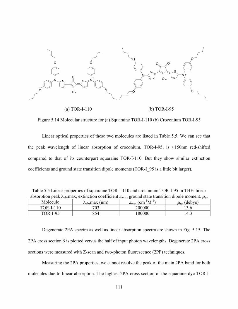
SSO

O

NN

O

O

O

O-

+ O

OO

SN

O

O

SN

O

O

-+

(a) TOR-I-110 (b) TOR-I-95

Figure 5.14 Molecular structure for (a) Squaraine TOR-I-110 (b) Croconium TOR-I-95

Linear optical properties of these two molecules are listed in Table 5.5. We can see that

the peak wavelength of linear absorption of croconium, TOR-I-95, is ≈150nm red-shifted

compared to that of its counterpart squaraine TOR-I-110. But they show similar extinction

coefficients and ground state transition dipole moments (TOR-I_95 is a little bit larger).

Table 5.5 Linear properties of squaraine TOR-I-110 and croconium TOR-I-95 in THF: linear absorption peak λabsmax, extinction coefficient εmax, ground state transition dipole moment. µge

Molecule λabsmax (nm) εmax (cm-1M-1) µge (debye) TOR-I-110 703 200000 13.6 TOR-I-95 854 180000 14.3

Degenerate 2PA spectra as well as linear absorption spectra are shown in Fig. 5.15. The

2PA cross section δ is plotted versus the half of input photon wavelengths. Degenerate 2PA cross

sections were measured with Z-scan and two-photon fluorescence (2PF) techniques.

Measuring the 2PA properties, we cannot resolve the peak of the main 2PA band for both

molecules due to linear absorption. The highest 2PA cross section of the squaraine dye TOR-I-

111

110 observed by experiment is much larger than that of croconium TOR-I-95. The reason for this

difference is still under study. In general, croconium dyes are a type of PD, and their 2PA

properties should be very similar to PDs. Here we observed that the relationships of both linear

and 2PA properties between SD and croconium dyes with analogous structures are similar to the

relationships between SDs and PDs discussed in Section 5.2.

300 400 500 600 700 800 900 10000

1500

3000

4500

6000

7500 TOR-I-110 TOR-I-95

2PA

cro

ss s

ectio

n (G

M)

Wavelength (nm)

0

50000

100000

150000

200000

Ext

inct

ion

coef

ficie

nt (c

m-1M

-1)4 3.5 3 2.5 2 1.5

Energy (eV)

Figure 5.15 2PA spectra for squaraine TOR-I-110 and croconium TOR-I-95. Linear spectra also are plotted for comparison.

5.5.2 Squaraine Vs Tetraon

We also compared the squaraine dye SD 2243 and tetraon dye TOD 2765. They are

synthesized at the Institute of Organic Chemistry, National Academy of Sciences, Ukraine.

Molecular structures are shown in Fig. 5.16. They have the same terminal groups. SD 2243 has a

squarylium acceptor core at the center of the conjugated chain, but TOD 2765 has a C6H12O4

acceptor core at the center that separates the conjugated chain of the left part of the molecule

from the right part. The effective conjugation length of TOD 2765 is shorter than that of SD

112

2243 because the central structure in the Tetraon breaks the conjugation chain connected from

the left to the right.

Nn-C4H9

CH3

CH3 O

O

N

CH3

CH3

n-C4H9

+

-

OO

OONn-C4H9

CH3CH3N

n-C4H9

CH3 CH3

(a) SD 2243 (b) TOD 2765

Figure 5.16 Molecular structure for (a) Squaraine dye SD 2243 and (b) Tetraon dye TOD 2765.

The linear optical properties of SD 2243 and TOD 2765 are summarized in Table 5.6.

Due to the shorter effective length of TOD 2765, we can see that the linear absorption band of

TOD 2765 is blue-shifted ≈ 60nm compared to SD 2243, and the ground state transition dipole

moment µ01 for TOD 2765 is smaller than that of SD2243. TOD 2765 also exhibits a stronger

linear absorption vibrational shoulder shown in Fig. 5.17.

Table 5.6 Linear properties of squaraine SD 2243 in CH2CL2 and tetraon TOD 2765 in ethanol: linear absorption peak λabsmax, extinction coefficient εmax and ground state transition dipole

moment µ01

Molecule λabsmax (nm) εmax (cm-1M-1) µ01 (debye) SD 2243 668 345000 13.8

TOD 2765 624 230900 13.0

The 2PA spectra of SD 2243 in CH2CL2 and TOD 2765 in ethanol are shown in Fig. 5.17.

The 2PA cross-section δ is plotted versus the half of input photon wavelengths. 2PA spectra are

measured by Z-scan and two-photon fluorescence (2PF).

113

We experimentally observed three 2PA bands for SD 2243 (δmax1 ≈ 80 GM at ≈ 615nm,

δmax2 ≈ 1000 GM at ≈ 440nm and δmax3 > 8000 GM at wavelengths shorter than 375nm),

however, we observed four 2PA bands for TOD 2765 (δmax1 ≈ 130 GM at ≈ 550 nm, δmax2 ≈ 877

GM at ≈ 483 nm, δmax3 ≈ 2700 GM at ≈ 410nm and δmax4 > 8000 GM at wavelengths shorter

than 340nm). Similar to linear absorption, 2PA bands of TOD 2765 are also blue-shifted

compared to those of SD 2243. We cannot resolve the peak of the 2PA band at shorter

wavelengths due to linear absorption. We conclude, based experimental data, that the

introduction of C6H12O4 at the center of the conjugated chain in TOD 2765 further increases the

density of electronic transitions between the linear absorption band and its “double resonance”

position. The molecular orbitals associated with this could be revealed by undergoing quantum

chemical calculations.

300 400 500 600 7000

2000

4000

6000

8000

10000

12000 SD2243 in CH2Cl2 TOD2765 in Ethanol

2PA

cro

ss s

ectio

n (G

M)

Wavelength (nm)

0

100000

200000

300000

Ext

inct

ion

coef

ficie

nt (c

m-1M

-1)4 3.5 3 2.5 2

Energy (eV)

Figure 5.17 2PA spectra for squaraine SD 2243 in CH2CL2 and tetraon TOD 2765 in Ethnaol. Linear spectra also are plotted for comparison.

114

5.6 Relations of one-photon anisotropy to 2PA spectra

5.6.1 One-photon excitation fluorescence anisotropy

Steady-state one-photon excitation fluorescence anisotropy spectra of organic molecules

were measured in high viscosity solvents to avoid reorientation of molecules, and in low

concentration solutions (peak OD < 0.1) to avoid reabsorption of fluorescence, with a PTI

Quantamaster Spectrofluorimeter. The experimental setup is shown as below:

Light source

Detector

Molecules

||I

⊥I

x

y

zL-Format experiment

polarizer

Light source

Detector

Molecules

||I

⊥I||I

⊥I

x

y

zL-Format experiment

polarizer

Figure 5.18 Experiment setup for one-photon and two-photon excitation fluorescence anisotropy measurement

The solutions of molecules are excited with vertically polarized light. One then measures

the intensity of the fluorescence emission through a polarizer at 90 degree (L-format

configuration) with the detector. When the emission polarizer is oriented parallel (||) to the

direction of the polarized excitation, the observed intensity is referred as I||. Likewise, when the

polarizer is perpendicular (⊥) to the excitation polarization, the intensity is called I⊥.

115

It is well-known that the excitation anisotropy spectrum, r(λ), can be calculated as a

function of the excitation wavelength λ at a fixed emission wavelength, usually near a

fluorescence maximum:

)(2)(

)()()(//

//

λλλλλ

⊥

⊥

+−

=II

IIr (5.3)

where and are the fluorescence intensities polarized parallel and perpendicular to the

excitation light [39].

//I ⊥I

One-photon anisotropy measurements can give information about the spectral position

and orientation of the transition dipole moments from the ground (S0) to the first (S1) and higher

(Sn) excited-states relative to the orientation of the emission dipole moment. The angle between

the absorption and emission dipole moments (β) can be determined from one-photon anisotropy,

2

1cos3 2

1−

=β

PAr (5.4)

In the range: , one-photon anisotropy ranges between, 00 090 ≤≤ β 4.02.0 1 ≤≤− PAr

5.6.2 Polymethine dyes

Here we show experimental results for three typical polymethine dyes with different

terminal groups: PD 2350, PD 2646 and PD 2630. The molecular structures are shown in Fig.

5.19. The 2PA cross section is plotted versus the wavelengths equal to half of input photon

wavelengths. One-photon excitation fluorescence anisotropy (all three molecules in Glycerol)

and degenerate 2PA spectra (all three molecules in ethanol), as well as linear absorption spectra

are shown in Fig; 5.20. All three PDs show strong correlation between one-photon anisotropy

spectra and 2PA spectra.

116

PD 2350 PD 2646 PD 2630

N

CH3CH3

N

CH3 CH3

C2H5 C2H5

p-CH3C6H4SO3

+

-

N

CH3

CH3

C3H7

NC3H7

CH3

CH3

I

+ S

NCH3

S

NCH3

CH3C6H4SO3

+

-

PD 2350 PD 2646 PD 2630

N

CH3CH3

N

CH3 CH3

C2H5 C2H5

p-CH3C6H4SO3

+

-

N

CH3

CH3

C3H7

NC3H7

CH3

CH3

I

+ S

NCH3

S

NCH3

CH3C6H4SO3

+

-

Figure 5.19 Molecular structures for polymethine dyes: PD 2350, PD 2646 and PD 2630

Analysis of one-photon excitation fluorescence anisotropy, r(λ), for PD 2350 revealed

the alternation of the allowed and forbidden (by symmetry) one-photon transitions. One-photon

forbidden transitions, as transitions between states of the same symmetry, can indicate a possible

position of 2PA bands. Shown in Fig. 5.20 (a), the first dip in r(λ) was observed at 412 nm (r1PA

= 0.22) corresponding to the angle β ≈ 330 between µ01 and µ10. However, the peak of 2PA for

PD 2350 is shifted to the blue region by ≈ 22 nm relative to this anisotropy dip. A second dip in

r(λ) at 330 nm (r1PA ≈ 0) corresponds to the angle β ≈ 550. Since this wavelength is almost

exactly half that of the absorption peak in the S0 → S1 transition, degenerate 2PA into this band

would be enhanced by an intermediate state resonance [56]. However, as we observed from Fig.

5.20, this “double resonance” cannot be experimentally reached by 2PA due to the influence of

the tail in the linear absorption band.

117

300 400 500 600 700

0

200

400

600

800

1000

1200 2PA

2PA

cro

ss s

ectio

n (G

M)

Wavelength (nm)

Linear Abs

0.0

0.1

0.2

0.3

0.4

0.5

0.6

One-photon anisotropy

One

-pho

ton

anis

otro

py

4 3.5 3 2.5 2Energy (eV)

(a) PD 2350

300 400 500 600 700 800

0

200

400

600

800 2PA

2PA

cro

ss s

ectio

n (G

M)

Wavelength (nm)

Linear Abs

-0.10.00.10.20.30.40.50.6

One-photon anisotropy

One

-pho

ton

anis

otro

py

4.5 4 3.5 3 2.5 2Energy (eV)

(b) PD 2646

300 400 500 600 700 800

0

500

1000

1500

2000 2PA

2PA

cro

ss s

ectio

n (G

M)

Wavelength (nm)

Linear Abs

0.0

0.1

0.2

0.3

0.4

0.5 One-photon anisotropy

One

-pho

ton

anis

otro

py

4.5 4 3.5 3 2.5 2Energy (eV)

(c) PD 2630

Figure 5.20 One-photon excitation fluorescence anisotropy and 2PA spectra for three PDs with different terminal groups. Linear spectra also are plotted for comparison.

118

Let’s go back to see the quantum chemical calculations in Section 5.3 (Fig. 5.6) to reveal

the origin of this correlation. As shown in Fig. 5.6 for PD 2350, there are two identical HOMO-1s

of the isolated TGs (with charge localization only at TGs, see in Fig. 5.5). Introduction of the

symmetrical terminal groups leads to the formation of doubly degenerate configurations resulting

in their energies splitting. After splitting, one of these MOs typically mixes with the orbital of the

chain producing a delocalized molecule orbital, HOMO-2, shown in Fig. 5.6 and Fig. 5.7. The

transition from HOMO-2 to LUMO (1A1 → 2B1, S0 → S3 shown in Table 5.3) can be seen in

one-photon absorption (non zero transition dipole moment). The peak of this one-photon

transition band (410nm in Table 5.3) corresponds to a dip in the one-photon anisotropy spectrum

(412nm in Fig. 5.20 (a)).

The other MO remains localized at the benzene rings of the TGs (see HOMO-3 shown in

Fig. 5.6 and Fig. 5.7). The existence of this local molecular orbital is of great importance for 2PA.

The transition from HOMO-3 to LUMO (1A1→ 1A3, S0 → S4 in Table 5.3) gives zero overlap

(see in Fig.5.7), thus it requires an intermediate (HOMO) state and forms a two-photon absorbing

transition. Our understanding is that the localized – delocalized electronic transition, such as

HOMO - 3 → LUMO, which appears in the energy interval between the S0 → S1 and its “double

resonance”, is responsible for the strong 2PA band with peak at 390nm.

Similar to PD 2350, for PD 2630 in Fig. 5.20 (c) there is a shift of ≈ 13 nm between the

second 2PA peak (440nm) and the first one photon excitation fluorescence anisotropy dip

(453nm). The splitting energy for polymethine dyes with indolium and benzoindolium TGs is

larger. Therefore, for these molecules, the 2PA peaks are blue-shifted relative to the anisotropy

dips (see Appendix B).

119

The energy splitting depends on the energy position of the orbitals from the isolated

terminal groups relative to the chain orbitals and thus on the terminal groups’ structure (length of

conjugation, donor strength). A small splitting energy leads to approximate overlap between one-

photon anisotropy dips and the positions of the 2PA peaks. Figure5.20 (b) shows a strong

correlation between the 2PA peak and the one-photon anisotropy dip for PD 2646 with the

thiazolium terminal groups. The same trend was observed for all other polymethine molecules

(see Appendix B).

5.6.3 Squaraine dyes

We also compared one-photon anisotropy spectra with 2PA spectra for two squaraine dyes.

Experimental data for other squaraines can be found at Appendix B. Molecular structures are

shown in Fig. 5.21. SD 2577 was synthesized at the Institute of Organic Chemistry, National

Academy of Sciences, Ukraine. SC-V-21c was synthesized by Seth Marder’s group at the Georgia

Institute of Technology, Atlanta. The one-photon excitation anisotropy spectra (SD 2577 in

Glycerol, SC-V-21c in Silicon Oil) as well as degenerate 2PA spectra (SD 2577 in ethanol, and

SC-V-21c in CH2CL2) are shown in Fig. 5.22. The 2PA cross section is plotted versus the

wavelengths equal to half of input photon wavelengths.

NO

OCH3CH3

CH3CH3

NC3H7

C3H7

+

N

N O

ON

N

+-

NO

OCH3CH3

CH3CH3

NC3H7

C3H7

+

N

N O

ON

N

+-

(a) SD 2577 (b) SC-V-21c

Figure 5.21 Molecular structures for squaraine dyes (a) SD 2577 (b) SC-V-21c

120

300 400 500 600 700

0

1500

3000

4500

6000 2PA

2PA

cro

ss s

ectio

n (G

M)

Wavelength (nm)

Linear Abs

0.0

0.1

0.2

0.3

0.4

0.5


One

-pho

ton

anis

otro

py

5 4 3 2Energy (eV)

(a) SD 2577

300 400 500 600 700 800 9000

10000

20000

30000

40000

2PA

cro

ss s

ectio

n (G

M)

Wavelength (nm)

2PA Linear Abs

-0.10.00.10.20.30.40.50.6

One-photon anisotropy (1) One-photon anisotropy (2)

One

-pho

ton

anis

otro

py

4 3 2Energy (eV)

(b) SC-V-21c

Figure 5.22 One-photon excitation fluorescence anisotropy and 2PA spectra for two SDs: (a) SD 2577 (b) SC-V-21c. There are two curves for one-photon anisotropy spectra: (1) measured by the visible detector, PMT R928b (2) measured by the near IR PMT. Linear spectra are also plotted

for comparison.

121

The 2PA spectrum for SD2577 can be directly mapped onto the one-photon anisotropy

function r(λ). The observed dips of one-photon anisotropy at 410 nm (r1PA = 0.22, β ≈ 330) and

at 345 nm (r1PA = 0.13, β ≈ 420) correspond to the peak positions of the 2PA bands. Analogous

to PD 2350, the last dip at 309 nm (r1PA = 0.06, β ≈ 490), corresponding to a position of twice the

energy of the main allowed S0 → S1 absorption band (or “double resonance” position) is

obscured by one-photon absorption.

We also observed this strong correlation for SC-V-21c. The observed dips of one-photon

anisotropy at 460nm and at 546nm correspond to the peak positions of the experimentally

observed 2PA bands as well.

Explanation for this correlation for SDs is not so straightforward as for PDs. More

research needs to be carried out to understand this.

122

CHAPTER 6 TWO-PHOTON EXCITATION FLUORESCENCE ANISOTROPY

6.1 Introduction

A much less investigated approach for understanding the 2PA properties of organic

molecules is the study of one-photon and two-photon excitation fluorescence anisotropy. Such

studies can give additional information about the nature of intermediate states and the molecular

symmetry. It is commonly known that one-photon excitation fluorescence anisotropy

measurements, especially linked to quantum-chemical calculations, can reveal the spectral

positions and orientations of the transition dipole moments from the ground to the first, µ01, and

higher excited-states, µ0n, relative to the orientation of the emission dipole moment, µ10, which

cannot be obtained from one-photon absorption spectra, but is important for understanding 2PA

processes.

It was shown theoretically [79] that the range of two-photon anisotropy, , values is

much broader than for indicating potential advantages of two-photon excitation. In practice,

as will be shown in this dissertation and in a previous paper [80], spectra for many organic

dyes are almost wavelength independent within several electronic transitions. It is necessary to

note that literature studies are very limited. Most of the measurements were performed only

within one electronic band, and their analysis is usually directed at a comparison of the values of

and . An overview of the existing experimental data was presented by Lakowicz and

Gryczynski in Ref. [81]. However, to our knowledge, an explanation of the wavelength

PAr2

PAr1

PAr2

PAr2

PAr1 PAr2

123

independent behavior of as well as its potential for understanding the properties of 2PA has

not been reported.

PAr2

6.2 Experimental setup

The light source for one-photon excitation fluorescence anisotropy measurements is a

Xenon lamp. However the light source for two-photon excitation fluorescence anisotropy

measurements is our Clark-MXR, CPA2010, Ti:Sapphire amplified femtosecond laser system

followed by an optical parametric generator/amplifier (model TOPAS 4/800, Light Conversion)

providing laser pulses of 140 fs (FWHM) duration with 1 kHz repetition rate. Experimental setup

for two-photon excitation fluorescence anisotropy is same as that for one-photon anisotropy

shown in Fig. 5.18

The anisotropy of up-converted fluorescence of all molecules under two-photon

excitation was measured in 1 cm quartz cuvettes with the same PTI Quantamaster

Spectrofluorimeter and the same experimental configuration as shown in Fig .6.1. Special care

was taken to minimize reabsorption of the emission, especially for the dyes with a small Stokes

shift as, for example, for PDs with a typical Stokes shift of ≈ 15-20 nm. We controlled this

reabsorption by comparing the shape of up-converted fluorescence (usually red-shifted due to the

high concentration typically used for 2PA studies) with one-photon fluorescence obtained from

the diluted solution. We found experimentally that for all the molecules studied the up-converted

fluorescence at concentrations ≤ 10-5 M completely overlaps the one-photon fluorescence band,

confirming that reabsorption is negligible. Therefore, we used 10-5 M or smaller concentrations

124

for all two-photon anisotropy studies. The measurements and calculations of were

performed as described above in Eq. 6.2.

PAr2

6.3 Two-photon anisotropy: four-state and three-state model

Derivation of the formula for two-photon excitation fluorescence anisotropy is based on

two theoretical approaches. The first was made by P. R. Callis [82], who used McClain’s original

treatment for the two-photon absorption (2PA) tensor and added the fluorescence transition

dipole moment to develop the equation for the two-photon anisotropy function. The second

theoretical approach was made by P. Cronstrand et al [32]. They derived the equation for 2PA

cross section in a more general four-state/two-intermediate-level model taking into account the

influence of an additional second excitation channel.

We obtain the equation for the two-photon excitation fluorescence anisotropy in the

four-state/two-intermediate-state approximation shown in Fig. 6.2 (a). The assumptions are 1)

the two photons for excitation have identical photon energies and the same polarization

(degenerate 2PA case); 2) all transition dipole moments are in one plane, or planar molecule

assumption. In the final formula, should be expressed in terms of absorbing dipoles

PAr2

PAr2 01µ , n0µ ,

f1µ , nfµ (not their projections), angles α, β, γ, θ between transitions (α is the angle between

emission dipole moment f and isometric line of ground state transition dipole moment 01µ and

excited state transition dipole moment f1µ , β is the angle between transition dipole moments

01µ and n0µ , γ is the angle between ground state transition dipole moment 01µ and excited state

transition dipole moment f1µ , θ is the angle between transition dipole moments 01µ and n0µ in

125

Fig.6.2 (b)) and detuning energies 1E∆ , 2E∆ . After algebraic transformation, we can write the

expression (detailed derivation is shown in Appendix D):

)(7

8)(18

423

423321

2 KKKKKKK

r PA ++−+

= (6.3)

where )2

cos()2

cos(10121 αγαγµµ −+∆= fEK ;

)2

cos()2

cos(012 βαγθαγµµ −++−∆= nfnEK ;

)cos(cos 0110123 βθγµµγµµ −+∆+∆= nfnf EEK ;

]coscos)cos()[cos(2

)cos1()](cos1[

100121

221

201

22

2220

214

βθβγθγµµµµ

γµµβθγµµ

+−+∆∆+

++∆+−++∆=

nffn

fnfn

EE

EEK

X

µ01

µ0n

µ1f

µnf

ωh

sn

sf

s1∆E1

∆En

s0

µ1f

µ01

µ0n µnf

µ10ωh

sn

sf

s1∆E1

∆En

s0

µ1f

µ01

µ0n µnf

µ10

f

Y

β

γα

θφ

emβ

01βX

µ01

µ0n

µ1f

µnf

Y

β

γα

θφ

emβ

01β

f

(a) (b)

Figure 6.1 Four-state, two-intermediate level (S1 and Sn ), model for two-photon anisotropy, (a) energy states S0, S1, Sf and Sn diagram; (b) transition dipole moments schematic diagram

In case of the simplest three-state/one-intermediate-state model shown in Fig. 6.3 (α is

the angle between emission dipole moment f and isometric line of ground state transition dipole

moment 01µ and excited state transition dipole moment f1µ , γ is the angle between ground state

126

transition dipole moment 01µ and excited state transition dipole moment f1µ , αem is the angle

between emission dipole moment f and ground state transition dipole moment 01µ in Fig.6.3 (b)):

S0 → S1 and S1 → Sf (S1 is the only intermediate state and Sf is the final state), Eq. 6.3 can be

simplified to Eq. 6.4, which is the same as the formula derived in Ref. [82] using a 3-state model,

)1cos2(7

1cos7cos)2

cos()2

cos(182

2

2 +

+−+−=

γ

γγαγαγ

PAr (6.4)

The main difference between Eq. (6.3) and (6.4) is that in the three-state model, two-

photon anisotropy, , depends only on the mutual orientation (α and γ ) in 2D-space of three

transition dipole moment vectors participating in the 2PA process (µ

PAr2

01: S0 → S1, µ1f : S1 → Sf

and fem: S1 → S0), and does not depend on the values of the absorbing dipole moments and

detuning energy.

Sf

S1

S0

µ1f

µ01 fem

∆µ

Sf

S1

S0

µ1f

µ01 fem

∆µ

X

µ01

µ1f or ∆µ

fem

Y

γ

α

αem

X

µ01

µ1f or ∆µ

fem

Y

γ

α

αem

(a) (b)

Figure 6.2 Three-state one-intermediate level (S1) model for two-photon anisotropy: (a) energy states S0, S1, Sf diagram; (b) transition dipole moments schematic diagram

The angle αem = α + 2γ in Fig. 6.3 (b) is the angle of orientation of µ01 relative to the

orientation of fem, which could be calculated from the one-photon excitation anisotropy spectra.

127

If the absorbing dipole µ01 is parallel to µ1f, γ = 0 (αem=α) and the angle α becomes

equal to the angle between absorbing and emitting dipoles, then r reduces to the well-known

formula [39]:

7

2cos6 2

2−

= emPAr

α (6.5)

In the case of αem = 0°, reaches its maximum value 0.57. If αPAr2 em= 90°, the value of is

minimal: -0.29.

PAr2

6.4. Symmetric molecules

We measured two-photon excitation anisotropy spectra for most of the polymethine and

squaraine dyes (see Appendix B) synthesized at the Institute of Organic Chemistry, National

Academics of Sciences, Ukraine. Here, we choose only four polymethine dyes for our two-

photon excitation fluorescence anisotropy measurement and analysis. We also choose two

fluorene molecules synthesized by Kevin Belfield’s group in the Department of Chemistry,

University of Central Florida in Orlando for analysis. Three of them are symmetric molecules

(PD2350, PD3428 and Fluorene 2), the other three are asymmetric molecules (PD2665, Styryl 1

and Fluorene 1). The molecular structures of polymethine dyes are shown in Fig. 6.4, and the

molecule structures of two fluorene molecules are shown below in Fig. 6.5:

128

N

CH3

CH3

C3H7

NC3H7

CH3

CH3

I

+ NN

CH3 CH3

CH3CH3

+

ClO4-

N N

S

CH3

CH3CH3

C2H5 ClO4

+

-

S

N

NCH3

CH3C2H5

CH3C6H4SO3

+

-

PD 2350 PD 3428

PD 2665 Styryl_1

N

CH3

CH3

C3H7

NC3H7

CH3

CH3

I

+ NN

CH3 CH3

CH3CH3

+

ClO4-

N N

S

CH3

CH3CH3

C2H5 ClO4

+

-

S

N

NCH3

CH3C2H5

CH3C6H4SO3

+

-

PD 2350 PD 3428

PD 2665 Styryl_1 Figure 6.3 Molecular structures for polymethine dyes PD2350, PD3428, PD2665 and Styryl_1

NH

CO

CH3N

SC10H21 C10H21

N

SC2H5 C2H5

S

N

Fluorene 1 Fluorene 2

NH

CO

CH3N

SC10H21 C10H21

N

SC2H5 C2H5

S

N

Fluorene 1 Fluorene 2 Figure 6.4 Molecule structures of two fluorene derivatives for two-photon excitation

fluorescence anisotropy measurements.

The experimental results for the three symmetric molecules are shown in Fig. 6.6. For

comparison with linear absorption, 2PA and two-photon anisotropy spectra are presented as

functions of wavelength equal to half of input photon wavelengths.

129

300 400 500 600 700-0.2

-0.1

0.0

0.1

0.2

0.3

0.4

0.5

0.6

r 1PA, r

2PA

Wavelength (nm)

0

500

1000

1500

2PA

cro

ss s

ectio

n (G

M)

4 3 2

PD2350 4

3

2

2

1

Sum of Photons (eV)

300 400 500 600 700 800-0.2

-0.1

0.0

0.1

0.2

0.3

0.4

0.5

0.6

r 1PA, r

2PA

Wavelength (nm)

0

1000

2000

3000

4000

5000

2PA

cro

ss s

ectio

n (G

M)

5 4 3 2

PD3428

3

4

2

2

1

Sum of Photons (eV)

(a) (b)

250 300 350 400 450-0.2

-0.1

0.0

0.1

0.2

0.3

0.4

0.5

0.6

r 1PA, r

2PA

Wavelength (nm)

0

100

200

300

400

500

600Fluorene 2

2PA

cro

ss s

ectio

n (G

M)

4.5 4 3.5 3

4

3

2

1

Sum of Photons (eV)

(c)

Figure 6.5 (1) linear absorption, (2) 2PA, (3) one-photon fluorescence anisotropy and (4) two-photon fluorescence anisotropy spectra for symmetric molecules; (a) PD2350; (b) PD3428; (c)

Fluorene 2.

For both three-state (Eq. 6.4) and four-state models (Eq. 6.3), depends on angle α, or

α

PAr2

em = α + 2γ (angle between the absorbing dipole moment µ01 and emission dipole moment fem),

which can be calculated from the maximum value of the one-photon anisotropy . From Fig.

6.6, for all three symmetric molecules indicating that α

max1PAr

38.0max1 ≈PAr em does not exceed ~10°.

130

6.4.1.Analysis: Three-state model

Based on three-state model of Eq. 6.4, we can plot a set of curves for as a function

of γ ranging from 0° to 180° at several α

PAr2

em as shown in Fig. 6.7. All curves converge to a point

at γ = 90° independent of the value of α14.02 =PAr em.

For symmetric molecules, quantum-chemical theory predicts that for 2PA to S2 state, the

transition dipoles µ01 and µ12 are parallel γ = 0° (or anti-parallel γ=180°), for 2PA to the S1 state

µ01 and ∆µ are perpendicular γ = 90°. Thus from curve 3 (αem=10° do) in Fig. 6.7, the theoretical

value of ≈ 0.55 for 2PA to the SPAr2 2 state (γ = 0°) and 0.14 for 2PA to the S1 state (γ = 90°).

Compared with experimental data, we found that for PD 2350 and PD 3428, 49.047.02 −≈PAr

for both 2PA to S1 and S2 states, and contradicted the theoretical predictions. For fluorene 2, we

measured for both transitions, which is close to the theoretical value for 2PA to the

S

53.02 ≈PAr

2 state, but also disagrees with the theoretical result for 2PA to the S1 state.

0

0.10

0.20

0.30

0.40

0.50

0.60

0 20 40 60 80 100 120 140 160 180

4

4

23

2 11

γ (degree)

r 2PA

Figure 6.6 Two-photon anisotropy as a function of the angle γ with the three-state model at (1) αem=0° ; (2) 5°; (3) 10°; and (4) 20°.

131

In order to understand the reason for this disagreement between the three-level model and

experiments for symmetric molecules, we propose two ways as described in the next two

sections

6.4.2. Analysis: Four-state model

Here we go to a more complete four-state model with Eq. 6.3. As shown in Fig.6.2,

becomes a function of the mutual orientation (angles α, γ, β, θ ) in 2D-space of all 5 transition

dipoles participating in the 2PA process, and also a function of the magnitudes of the four

transition dipole moments and two detuning energies. We made this four-state model analysis

with molecule PD2350 (experimental data shown in Fig. 6.6 (a)).

PAr2

We assume that 2PA to S2 includes two simultaneous scenarios or channels: S0 → S1 then

S1 → S2 (first), and S0 → S4 then S4 → S2 (second), which is shown in Fig. 6.2 (a) where Sn = S4

and Sf=S2. The choice of S4 as the second intermediate state for PDs is connected with our

observation, taken from one-photon anisotropy spectra, that the angle β (between two scenarios

or between and ) is typically one of the largest angles (≈ 6001µ 04µ 0) among the measurable S0

→ Sn transitions. According to traditional quantum-chemical theories for symmetric molecules,

the transitions within each scenario can be anti-parallel ((γ = φ = 1800) or parallel (γ = φ = 00) to

each other, where γ is an angle inside of the first scenario (between µ01 and µ12), and φ is the

angle inside of the second scenario (between µ04 and µ42) (see in Fig. 6.2 (b)). The dependence of

upon the angle γ calculated by Eq. 6.3 is shown in Fig. 6.8(a). Typically, for polymethines,

the contribution of the second channel is small:

PAr2

12014204 µµµµ << , therefore, the curve in Fig. 6.8

(a) completely overlaps with curve 3 in Fig. 6.7 which is calculated by the three-state model. In

132

this case, depends mainly on γ and αPAr2 em, and does not change significantly with changes of β

and φ, which is shown in the 3D plot in Fig. 6.8(b).

0

0.1

0.2

0.3

0.4

0.5

0.6

0 20 40 60 80 100 120 140 160 180

γ (degree)

r 2PA

(a) (b)

Figure 6.7 (a) Two-photon anisotropy , calculated in the four-state model, as a function of γ. α

PAr2

em = 100; µ01 =13.5 D; µ12 = µ04 = µ42 = 1 D; β = 600; φ = 00 (or 1800); ∆E1 = 0.5 eV; ∆E2 = 2.5 eV. This curve coincides with curve 3 from Fig. 6.7 obtained from the three-state model. (b) 3D

picture of , calculated in the four-state model, as a function of β and φ for αPAr2 em = 100; µ01 =13.5 D; µ12 = µ04 = µ42 = 1 D; γ = 1800.

6.4.3. Analysis: Symmetry breaking of symmetric molecules

Since the more complete four-state model cannot explain the discrepancy between the

theory and experiments for symmetric molecules shown in Fig. 6.6 either, we tried to explain this

with the symmetry breaking of symmetric molecules.

For PD2350, based on calculations from the three-state model (Eq.6.4, and curve 3 in Fig.

6.7), in order to achieve 49.047.02 −≈PAr over two electronic transitions, which is what

experiments showed, the deviations of orientation of the participating dipoles should be ≈ 350 for

∆µ from the perpendicular “classical” orientation, and ≈ 170 for µ12 from the anti-parallel

133

“classical” orientation. These deviations could be due to ground-state symmetry breaking. This is

illustrated in Fig. 6.9.

Even a small contribution of an asymmetrical form can lead to non-equality in the charge

transfer from the terminal groups to the chain center, which will affect the orientation of the

transition moments. As shown in Fig. 6.9, this effect cannot essentially change the orientation of

the large S0 → S1 transition dipole moment since for both forms charge transfer occurs in the

direction of the chromophore. However, for other transition dipole moments, which are at least

one order of magnitude smaller, the difference in the charge transfer from the terminal groups to

the center of the chain can strongly affect their orientations. An especially strong effect can be

observed for the “perpendicular” (to S0 → S1) transitions, such as ∆µ, µ02 (S0 → S2), µ04 (S0 →

S4). It is seen that the asymmetrical charge transfer from the terminal groups can change the

direction of µ02 relative to µ01. However, we cannot predict how the deviation of µ02 will change

the “classical” orientation of µ12 (parallel or anti-parallel to µ01). Further development of

quantum-chemical theory is necessary.

The assumption about the ground-state symmetry breaking, affecting the orientations of

higher excited-state transition dipole moments relative to µ01, can explain why in one-photon

anisotropy measurements the “classical” minimal anisotropy value = -0.2, corresponding to

an angle α

PAr1

em = 900, has not been observed for PDs (also see this in Appendix B). The maximum

angles observed experimentally for the “perpendicular” transitions in PDs were 600 – 650.

134

+NC3H7

CH3CH3

C3H7

N

CH3H3C

µ02µ01

µ03

µ’02µ”

02

+NC3H7

CH3CH3

C3H7

N

CH3H3C

µ02µ01

µ03

µ’02µ”

02µ02

µ01µ03

µ’02µ”

02

µ01µ03

µ02µ”

02 µ’02

+N

C3H7

CH3CH3

C3H7

N

CH3H3C

µ01µ03

µ02µ”

02 µ’02

+N

C3H7

CH3CH3

C3H7

N

CH3H3C

+N

C3H7

CH3CH3

C3H7

N

CH3H3C

(a) (b)

Figure 6.8 Schematic presentation of the orientation of the transition dipole moments for (a) symmetrical and (b) asymmetrical forms of PD 2350. µ”

02 and µ’02 indicate a partial charge

transfer from each terminal group to the polymethine chromophore.

6.5. Asymmetric molecules

The experimental results for the three asymmetric molecules (PD2665, Styryl 1 and

Fluorene 1) are shown in Fig. 6.10 (a)-(c). For comparison with linear absorption, 2PA and two-

photon anisotropy spectra are presented as functions of wavelength equal to half of input photon

wavelengths.

We also compare experimental data with the three-state model (Eq. 6.4). Quantum-

chemical calculations performed for these molecules, show that µ01 and µ12 are oriented almost

parallel (angles γ are within 100) similar to the symmetrical molecules. However, ∆µ shows a

large deviation from an orientation perpendicular to µ01. These angles γ for Styryl 1, PD 2665

and fluorene 1 equal 260, 430 and 370 respectively. Substituting theseγ’s into the three-state

model or Eq. 6.4, as well as using the experimental value of αem = 100, which is the same for all

these molecules, we calculated that ≈ 0.55 - 0.56 for 2PA to both SPAr2 1 and S2 states. Thus, the

three-state model can be used to model the asymmetrical molecules for two-photon excitation

fluorescence anisotropy.

135

300 400 500 600 700-0.2

-0.1

0.0

0.1

0.2

0.3

0.4

0.5

0.6

r 1PA,

r 2PA

Wavelength (nm)

0

500

1000

1500

2000

2500

2PA

cro

ss s

ectio

n (G

M)

5 4 3 2

PD26654

3

2

2

1

Sum of Photons (eV)

250 300 350 400 450 500 550 600 650-0.2

-0.1

0.0

0.1

0.2

0.3

0.4

0.5

0.6

r 1PA,

r 2PA

Wavelength (nm)

0

100

200

300

400

500

600

700

800

2PA

cro

ss s

ectio

n (G

M)

5 4 3 2

Styryl 1

4

3

22

1

Sum of Photons (eV)

(a) (b)

250 300 350 400 450-0.2

-0.1

0.0

0.1

0.2

0.3

0.4

0.5

0.6

r 1PA, r

2PA

Wavelength (nm)

0.0

0.2

0.4

0.6

0.8

1.0

Nor

mal

ized

Abs

orpt

ion

4.5 4 3.5 3Fluorene 1

4

3

1

Sum of Photons (eV)

(c)

Figure 6.9 Linear absorption (1), 2PA spectra (2), one-photon anisotropy (3) and two-photon anisotropy (4) for asymmetric molecules: (a) PD2665; (b) Styryl 1; (c) Fluorene 1.

6.6 Why do we use the four-state model?

From the above analysis, we see that the three-state model works for asymmetric

molecules fairly well, but both three- and four-state models do not work for the symmetric

136

molecules we studied, and we have to introduce symmetry breaking to explain the lower

experimental value of for symmetrical molecules. So what is the benefit for us to have a

more complicated four-state model for two-photon excitation fluorescence anisotropy?

PAr2

Based on the four-state model, theoretically there is a way to decrease closer to the

experimental values for symmetric molecules without introducing symmetry breaking (means

that we can keep the parallel or anti-parallel “classical” orientation of transitions inside each

channel for symmetric molecules).

PAr2

0 45 90 135 180 225 270 315 360-0.3-0.2-0.10.00.10.20.30.40.50.6

32

1

r 2PA

γ (degree)

(a) (b)

Figure 6.10 (a) Two-photon anisotropy for 2PA to SPAr2 2 state of PD2350, calculated in the four-state model, as a function of γ. Curve 1: αem = 100; β = 600; φ = 00 (or 1800); ∆E1 = 0.5 eV; ∆E2

= 2.5 eV; µ01 =13.5 D; µ12 =1D; µ04 = µ42 = 1 D. Curve 2 and 3: αem = 100; β = 600; ∆E1 = 0.5 eV; ∆E2 = 2.5 eV; µ01 =13.5 D; µ12 = 1 D; µ04 = µ42 = 6 D; φ = 00 (for curve 2) and φ = 1800 (for

curve 3). (b) 3D plot of , as functions of β, φ , with αPAr2 em = 100; γ = 1800; ∆E1 = 0.5 eV; ∆E2 = 2.5 eV; µ01 =13.5 D; µ12 = 1 D; µ04 = µ42 = 6 D

For this purpose we consider an increase of the contribution of the second channel. Fig.

6.11 (a) (curves 2 and 3) demonstrates these results for the case 12014204 µµµµ ≥ (µ01 =13.5 D,

µ12 = 1 D, µ04 = µ42 = 6 D). The 3D plot of , calculated in the four-state model, as functions PAr2

137

of β, φ at an increased contribution of the second channel, is presented in Fig. 6.11 (b), which

are compared with Fig.6.8 for µ04 = µ42 = 1D.

It is important to note that in contrast to the PDs studied in this dissertation, some

molecules from other classes of organic compounds possess strong transitions to the second or

higher excited states with dipole moments comparable to 01µ . For example, the symmetrical 9,9-

didecyl-2,7-bis-(N,N-diphenylamino)fluorene, reported in [76], shows relatively large transition

dipole moments (up to 6 debye) to the higher excited-states compared to the ground state

transition dipole moment 01µ = 8 debye. Its molecular parameters, revealed from quantum-

chemical calculations and substituted into the four-state model or Eq. 6.3, give ≈ 0.27

without involving symmetry breaking, which is close to its experimental value. This confirms

that the four-state model can be used for the explanation of into the S

PAr2

PAr2 1 and S2 states, if the

contribution of the effective second channel to 2PA is comparable with the contribution of the

first one.

For the polymethine molecules, this case may be achieved by considering the second

channel as a superposition of all possible channels oriented at relatively large angles to the first

excitation channel.

In addition, although based on the three-state model, does not depend on detuning

energy ∆E, or pump photon energy. The four-state model provides us a chance to study the

wavelength dependence of by changing the detuning energy. Figure 6.12 shows the two-

photon excitation anisotropy for PD2350 based on the four-state model as a function of

wavelength equal to half of input photon wavelength. By including a symmetry breaking effect,

PAr2

PAr2

PAr2

138

we could get the two-photon excitation fluorescence spectrum, which agrees with the

experimentally observed flat spectra. PAr2

Figure 6.11 Calculated wavelength dependence of under 2PA to SPAr2 1 state (1) and 2PA to S2 state (2) based on the four-state model. Molecular parameters for (1) are: αem = 100; µ01 =13.5 D; ∆µ = 0.6; µ02 = 1.2 D; µ21 = 1 D; φ = 900; β = 320; γ = 550. Molecular parameters for (2) are: αem

= 100; µ01 =13.5 D; µ12 = 1 D; µ04 = µ42 = 1 D; φ = 1800; β = 600; γ = 1630.

Although we can understand two-photon anisotropy having the same value within one

electronic transition based on the theoretical models, we still do not quite understand the

fundamental reason why two-photon anisotropy keeps the same value over several electronic

transitions for symmetric molecules, so more analysis has to be made.

139

CHAPTER 7 CONCLUSIONS

7.1 Conclusions

In this dissertation, the relationships of molecular structures to linear and nonlinear

optical properties (especially 2PA properties) for polymethine and squaraine dyes are addressed.

Systematically altering the molecular structures provided an effective way to investigate the

correlations of structure to their optical properties, and then indicated the pathway to design

novel organic molecules exhibiting large nonlinearity and ultimately to make nonlinear optical

organic photonic devices for real applications. These studies include effects of molecular

symmetry, strength of donor terminal groups, conjugation length of the chromophore chain,

polarity of solvents, and bridge molecules within the chromophore chain. We also compared

polymethine, squaraine, croconium and tetraon dyes with similar structures to study the effects

of the different additions inserted within the chromophore chain on their NLO properties. We

used three different nonlinear spectroscopic techniques (Z-scan, two-photon fluorescence and

white-light continuum pump-probe) to obtain 2PA spectra, revealing 2PA bands, and to confirm

the experimental data by comparing the results from different methods. Two-photon excitation

fluorescence anisotropy spectra were measured through several 2PA transitions. This is the first

time such measurement have been reported to our knowledge.

To understand the structure-property relationships observed from these experiments, we

used a simplified three-level model based on the 2PA tensor method to fit experimental 2PA

spectra to reveal the critical parameters for 2PA. Quantum chemical calculations help us

140

understand the evolution of molecular orbitals with changing to the structures, and transitions

between MOs which are responsible for observed linear and 2PA bands.

The conclusions related to the correlations of the molecular structures to their 2PA

properties are summarized below:

1) Symmetry: Symmetrical PDs and SDs show negligible 2PA into the first excited state, or

linear absorption band. But asymmetric molecules clearly show 2PA into any excited

state. Both symmetric and asymmetric PDs as well as SDs exhibit a weak 2PA band at

the vibrational shoulder of the linear absorption spectra, i.e.2PA from the ground state to

the higher lying vibration bands of the first excited state. Symmetry breaking is clearly

indicated for symmetric molecules by this 2PA band. The origin of the symmetry

breaking was investigated (see sections 4 and 9)).

2) Terminal Groups: Three molecules with different terminal groups (Thiazolium,

Indolium, Benzoindolium) and the same conjugation length were compared for their 2PA

properties. PD 2630 with the strongest donor benzoindolium terminal group exhibits red-

shifted linear and 2PA spectra, and the beginning of a third and stronger 2PA band can be

observed experimentally. Comparing 2PA properties of PD 200 and PD 2761 provides us

some insight about the effect of conjugation strcture in the terminal group on the linear

and nonlinear properties.

3) Conjugation Length: Increasing the conjugation length of the chromophore chain red-

shifts both the linear and 2PA bands, as well as increasing the 2PA cross section due to

increases of ground state transition dipole moments and decreases of detuning energies.

4) Polarity of Solvents: A way to study the symmetry breaking of symmetric molecules is

to study 2PA of molecules in solvents of different polarity. Experimental results indicated

141

two possible origins for this symmetry breaking. One is vibronic coupling due to the

vibrational shoulder in the linear absorption. The other is the existence of an

asymmetrical charge distribution in the symmetric molecules.

5) Bridge: Inserting a benzene bridge into the chromophore chain can protect the symmetric

molecules from symmetry breaking. Thus, we observed that the 2PA cross sections of

this weak 2PA band is smaller for bridged symmetric PDs than unbridged symmetric PDs.

6) Polymethines and Squaraines: SDs exhibited much larger experimentally observable

2PA cross sections than PDs having the same terminal groups and similar conjugation

length. Quantum chemical calculations showed that forming PDs by putting terminal

groups on the chromophore chain increases the density of occupied molecular orbitals,

thus increases electronic transitions for 2PA. Quantum chemical calculations also showed

that forming SDs by inserting a squarylium core into PDs further increases the density of

unoccupied molecular orbitals, thus the electronic transitions. Thus, combining with

narrower linear absorption bands, SDs move more 2PA bands with larger 2PA cross

sections into the experimentally observable region before being obscured by linear

absorption. Near IR absorbing squaraine dyes exhibit extremely large 2PA cross sections

(≈ 30000GM).

7) Squaraine, Croconium and Tetraon: Inserting different additions into the chromophore

chain forms squaraine (C4O2), Croconium (C5O3) and Tetraon (C6O4) dyes. Croconium

exhibits much smaller 2PA than squaraine, and tetraon dyes show similar large 2PA as

squaraine, but exhibits more 2PA bands than squaraines indicating an increase of the

number of electronic transitions.

142

8) One-photon Fluorescence Anisotropy: Our experimental results indicate the strong

correlation between one-photon excitation fluorescence anisotropy spectra and 2PA

spectra for symmetric PDs. Quantum chemical calculations show that this correlation

comes from energy splitting of molecular orbitals of two identical terminal groups. After

splitting, one molecular orbital corresponds to a one-photon transition, and the other

molecular orbital corresponds to a two-photon transition. And this splitting energy

depends on the structure of the terminal groups. For symmetric SDs, this correlation is

also observed.

9) Two-photon Fluorescence Anisotropy: Two-photon excitation fluorescence anisotropy

spectra for several 2PA bands are measured experimentally for the first time. A

theoretical model based on a four-level, two-intermediate-state model is developed. The

observed deviation of the two photon anisotropy from the theoretical prediction for

symmetric molecules indicates the existence of symmetry breaking.

7.2 Future work

From the conclusions listed above, a few potential research are are proposed:

1) The conjugation structure of terminal groups will increase the effective conjugation

length of molecules. The effect of conjugation length in the terminal groups on 2PA is

still an ongoing research project. I will propose to try to quantitatively describe the

donor/acceptor strength of different terminal groups, which will help to separate the

contributions of donor/acceptor strength in TGs from conjugation structure in TGs on the

2PA properties of the molecules.

143

2) To investigate the nature of symmetry breaking we need more experiments performed.

Linear absorption of long polymethine molecules (such as PD 1659) exhibits a strong

dependence on the polarity of solvents. Some short molecules exhibit less of this

dependence. It is proposed to measure 2PA of long molecules in solvents of different

polarity to study the effects of the asymmetric form in symmetric molecules on 2PA

However, two issues make this measurement difficult. One is that molecules with long

conjugation lengths will move the linear absorption band as well as the fluorescence

spectrum into the NIR region. Only the Z-scan technique can study the weak 2PA band at

the vibronic shoulder of the linear absorption band. The other is that the solubility of

symmetric molecules strongly depends on the polarity of the solvent, which makes it

impossible to prepare high concentration solutions for all solvents for Z-scan

measurements. Being able to use the very sensitive 2PF method becomes crucial for this

study.

3) Quantum chemical calculations need to be performed to understand the difference in 2PA

properties of squaraine, croconium and tetraon for optimizing molecules for 2PA

applications in the future.

4) The value of two-photon excitation fluorescence anisotropy is experimentally observed to

be constant for several 2PA bands for all the molecules we studied. We can explain this

for asymmetric molecules based on a three-level model. However we cannot explain this

phenomenon for symmetric molecules with three-level and four-level models. More

theoretical study on this is proposed.

144

APPENDIX A CGS AND SI UNIT

145

In chapter two, we derived the formula for the imaginary part of χ(3) in SI units. But when

we used the relation for the 2PA cross section and transition dipole moments to fit experimental

2PA spectra, we use a formula in CGS units because usually transition dipole moments are

expressed with units of debye (D) that belongs to CGS unit.

The CGS unit system is an abbreviation for the centimeter-gram-second system, which

uses the centimeter, gram and second for length, mass and time. The units most used parameters

for 2PA cross section theory are expressed in SI and CGS units listed in Table A.1.

Table A.1 Relationship of CGS to SI unit CGS Definition SI

Length centimeter 1 cm = 10-2 m Mass Gram 1 g = 10-3 kg Time Second 1 s = 1 s Energy Erg 1 erg = 1 g • cm2/s2 = 10-7 J Charge Esu 1 esu = 1 (g • cm3/s2)1/2 = 3.3356×10-10 C Dipole moment debye (D) 1 D = 1 10-18 cm • esu = 3.3356×10-10 C • m

We used Eq. 2.54 in Chapter 2 to fit the 2PA spectra of polymethine and squaraine

molecules. We calculated the constant and changed Eq. 2.54 into the Eq. 2.57 for practical use,

where the 2PA cross section is in units of GM (10-50 cm4 • s/molecule), all energies are input

with units of eV and all dipole moments are input with units of debye (D). The derivation for this

equation is shown below to verify the units validity and calculated constant in front.

146

[ ][ ] [ ] [ ]

[ ][ ] [ ] [ ] [ ]

[ ][ ] [ ] [ ]

[ ][ ] [ ] [ ]

[ ][ ] [ ] [ ]

[ ][ ] [ ] [ ]

[ ][ ] [ ] [ ]

[ ][ ] [ ] [ ]

[ ][ ] [ ] [ ]

[ ][ ] [ ] [ ]

[ ]( )[ ] [ ] [ ]( )

[ ][ ] [ ] [ ]( ) ][

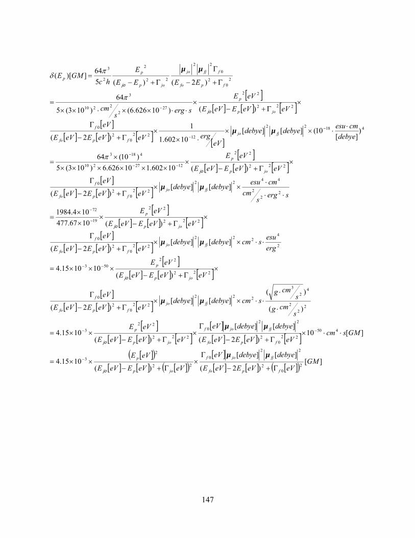
)2(

][][

)(1015.4

][10)2(

][][

)(1015.4

)(

)(][][

)2(

)(101015.4

][][)2(

)(1067.477104.1984

][][)2(

)(10602.110626.6)103(5)10(64

)][

10(][][10602.1

1)2(

)()10626.6()103(5

64

)2()(564])[(

20

2

22

0

22

23

45022

02

22

0

222

223

22

2

42

3

222

220

2

0

222

22503

2

4222

220

2

0

222

22

19

72

22

2

4422

220

2

0

222

22

1227210

4183

41822

12220

2

0

222

22

272

2210

3

20

2

0

22

22

2

2

3

GMeVeVEeVE

debyedebyeeV

eVeVEeVE

eVE

GMscmeVeVEeVE

debyedebyeeV

eVeVEeVE

eVE

scmg

scmg

scmdebyedebyeeVeVEeVE

eV

eVeVEeVE

eVE

ergesuscmdebyedebye

eVeVEeVE

eV

eVeVEeVE

eVE

sergscm

cmesudebyedebyeeVeVEeVE

eV

eVeVEeVE

eVE

debyecmesudebyedebye

eVergeVeVEeVE

eV

eVeVEeVE

eVE

sergscm

EEEE

E

hcGME

fpfo

fjjof

jop

p

fpfo

fjjof

jop

p

fjjofpfo

f

jop

p

fjjofpfo

f

jop

p

fjjofpfo

f

jop

p

fjjofpfo

f

jop

p

fpfo

ffjjo

jop

pp

Γ+−

Γ×

Γ+−××=

⋅⋅×Γ+−

Γ×

Γ+−××=

⋅

⋅⋅⋅××

Γ+−

Γ

×Γ+−

×××=

⋅⋅××Γ+−

Γ

×Γ+−

×××

=

⋅⋅

⋅××

Γ+−

Γ

×Γ+−

×××××××

×=

⋅⋅××

⋅××

Γ+−

Γ

×Γ+−

×⋅⋅××⋅××

=

Γ+−

Γ

Γ+−=

−

−−

−−

−

−

−−

−

−

−

−

µµ

µµ

µµ

µµ

µµ

µµ

µµ

jo

jo

jo

jo

jo

jo

jo

π

π

πδ

147

APPENDIX B EXPERIMENTAL DATA FOR MOLECULES FROM DR. OLGA V.

PRZHONSKA

148

We performed a comprehensive experimental study of PDs, SDs, and tetraon dye that are

synthesized at the Institute of Organic Chemistry, National Academy of Sciences, Ukraine. We

measured linear absorption spectra, one-photon fluorescence spectra, one-photon excitation

fluorescence anisotropy spectra, two-photon absorption spectra and two-photon excited

fluorescence anisotropy spectra. Below are listed experimental results for all molecules.

Molecular structures can be found in Fig. 4.2 and Fig. 5.1.

300 400 500 600 700

0

200

400

600

800

1000

2PA

2PA

cro

ss s

ectio

n (G

M)

Wavelength (nm)

1PA 1PF

-0.150.000.150.300.450.600.750.90

PD AF

One-photon anisotropy Two-photon anisotropy

Ani

sotro

py

4 3 2Energy (eV)

300 400 500 600 700 800

0

200

400

600

800

1000

1200

PD 2350

2PA

2PA

cros

s se

ctio

n (G

M)

Wavelength (nm)

1PA 1PF

0.00

0.15

0.30

0.45

0.60

0.75 One-photon anisotropy Two-photon anisotropy

Ani

sotro

py

4 3.5 3 2.5 2Energy (eV)

149

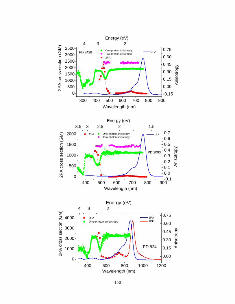
300 400 500 600 700 800 900

0500

100015002000250030003500

PD 3428 2PA

2PA

cro

ss s

ectio

n (G

M)

Wavelength (nm)

1PA

-0.15

0.00

0.15

0.30

0.45

0.60


Ani

sotro

py

4 3 2Energy (eV)

400 500 600 700 800 9000

500

1000

1500

2000 2PA

2PA

cro

ss s

ectio

n (G

M)

Wavelength (nm)

1PA

-0.10.00.10.20.30.40.50.60.7

PD 2093


Ani

sotro

py

3.5 3 2.5 2 1.5Energy (eV)

400 600 800 1000 12000

1000

2000

3000

4000 2PA

2PA

cro

ss s

ectio

n (G

M)

Wavelength (nm)

1PA 1PF

0.00

0.15

0.30

0.45

0.60


Ani

sotro

py

4 3 2

PD 824

Energy (eV)

150

300 400 500 600 7000

100

200

300

400

500

600

PD 25

2PA

2PA

cro

ss s

ectio

n (G

M)

Wavelength (nm)

1PA 1PF

0.00

0.15

0.30

0.45

0.60


Ani

sotro

py

4.5 4 3.5 3 2.5 2

Energy (eV)

300 400 500 600 700 800

0200400600800

10001200 2PA

PD 200

2PA

cros

s se

ctio

n (G

M)

Wavelength (nm)

1PA 1PF

-0.15

0.00

0.15

0.30

0.45

0.60


Anis

otro

py

4 3.5 3 2.5 2

Energy (eV)

300 400 500 600 700 8000

200

400

600

800

1000 2PA

2PA

cro

ss s

ectio

n (G

M)

Wavelength (nm)

1PA 1PF

-0.150.000.150.300.450.600.750.90

PD 2646 One-photon anisotropy Two-photon anisotropy

Anis

otro

py

4 3 2Energy (eV)

151

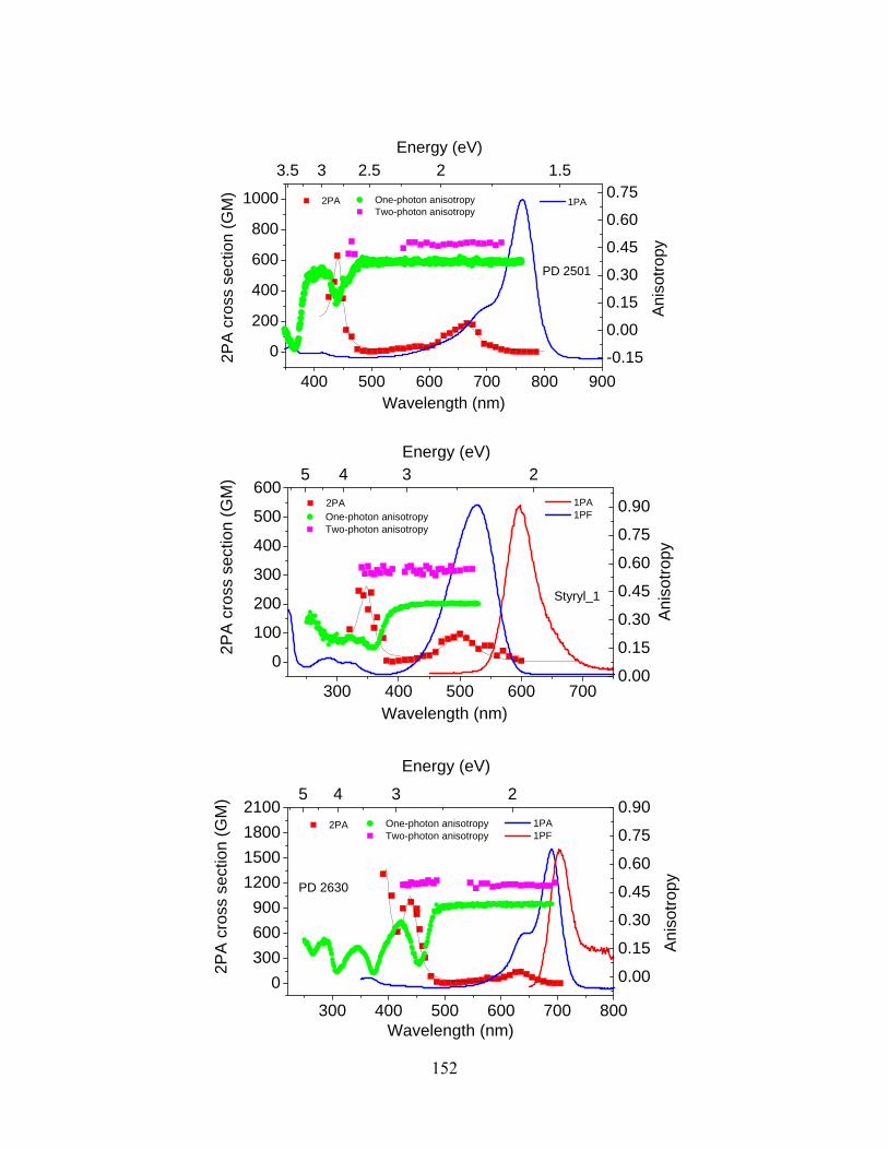
400 500 600 700 800 900

0

200

400

600

800

1000 2PA

2PA

cro

ss s

ectio

n (G

M)

Wavelength (nm)

1PA

-0.15

0.00

0.15

0.30

0.45

0.60

0.75

PD 2501


Ani

sotro

py

3.5 3 2.5 2 1.5Energy (eV)

300 400 500 600 700

0

100

200

300

400

500

600 2PA

2PA

cro

ss s

ectio

n (G

M)

Wavelength (nm)

1PA 1PF

0.00

0.15

0.30

0.45

0.60

0.75

0.90

Styryl_1


Ani

sotro

py

5 4 3 2Energy (eV)

300 400 500 600 700 800

0300600900

1200150018002100

2PA

2PA

cro

ss s

ectio

n (G

M)

Wavelength (nm)

1PA 1PF

0.00

0.15

0.30

0.45

0.60

0.75

0.90

PD 2630


Ani

sotro

py

5 4 3 2

Energy (eV)

152

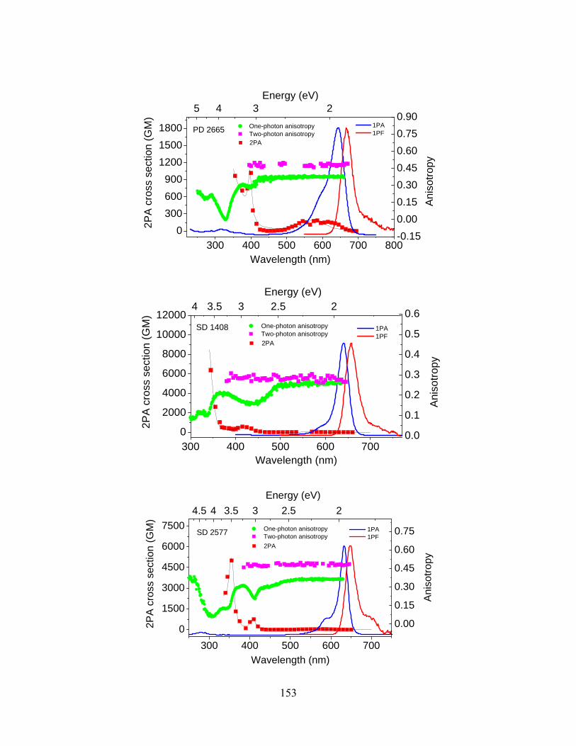
300 400 500 600 700 8000

300600900

120015001800

2PA2P

A c

ross

sec

tion

(GM

)

Wavelength (nm)

PD 2665 1PA 1PF

-0.150.000.150.300.450.600.750.90


Ani

sotro

py

5 4 3 2Energy (eV)

300 400 500 600 7000

2000

4000

6000

8000

10000

12000

2PA

2PA

cro

ss s

ectio

n (G

M)

Wavelength (nm)

1PA 1PF

0.0

0.1

0.2

0.3

0.4

0.5


Ani

sotro

py

4 3.5 3 2.5 2

SD 1408

Energy (eV)

300 400 500 600 7000

1500

3000

4500

6000

7500

2PA

2PA

cro

ss s

ectio

n (G

M)

Wavelength (nm)

1PA 1PF

0.00

0.15

0.30

0.45

0.60

0.75SD 2577 One-photon anisotropy Two-photon anisotropy

Ani

sotro

py

4.5 4 3.5 3 2.5 2Energy (eV)

153

300 400 500 600 700 800

0

3000

6000

9000

12000 SD 2243 2PA

2PA

cro

ss s

ectio

n (G

M)

Wavelength (nm)

0.0

0.1

0.2

0.3

0.4

0.5


Ani

sotro

py

4 3 2Energy (eV)

1PA 1PF

300 400 500 600 700 800

0

2000

4000

6000

8000

10000

12000TOD 2765

2PA

2PA

cro

ss s

ectio

n (G

M)

Wavelength (nm)

1PA 1PF

-0.150.000.150.300.450.600.750.90


Ani

sotro

py

5 4 3 2Energy (eV)

154

APPENDIX C EXPERIMENTAL DATA FOR MOLECULES FROM DR. SETH R.

MARDER’S GROUP

155

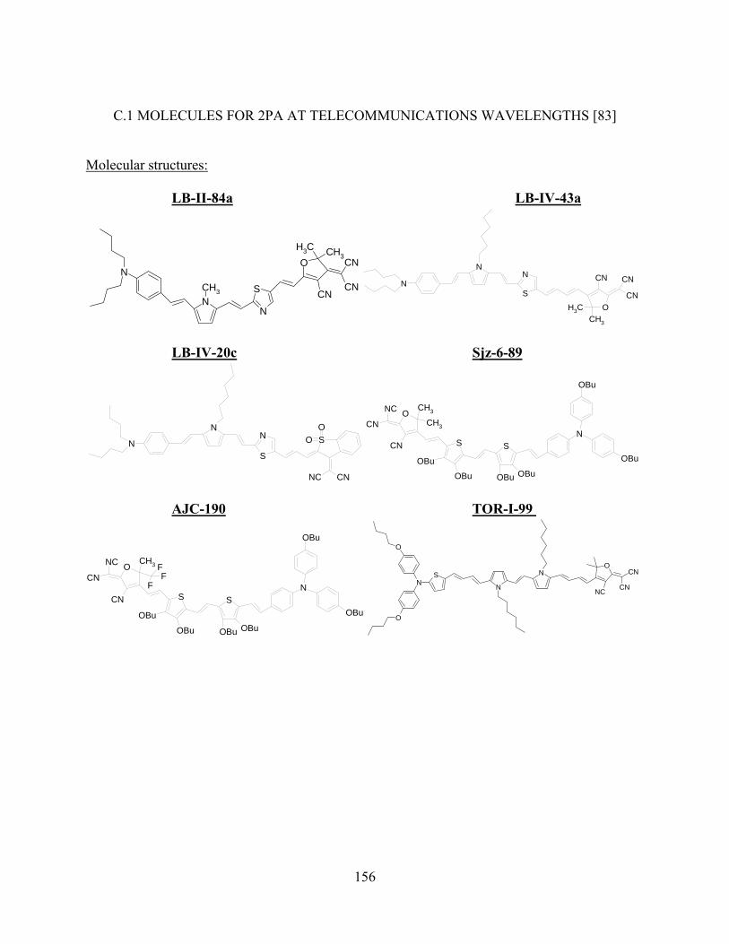
C.1 MOLECULES FOR 2PA AT TELECOMMUNICATIONS WAVELENGTHS [83]

Molecular structures:

LB-II-84a LB-IV-43a

NCH3 S

N

OCH3

CH3

NCN

CNCN

N

S

N

OCH3

CH3

CN CN

CNN

LB-IV-20c Sjz-6-89

N

S

N SO

O

CNNC

N SN

S

OBu

OBu

OCH3

CH3

CN

NC

CN

OBu

OBu

OBu OBu

AJC-190 TOR-I-99

SN

S

OBu

OBu

OCH3

CN

NC

CN

OBu

OBu

OBu OBu

FF

F N

NO

CN

CNNC

SN

O

O

156

LB-II-84a in THF

400 500 600 700 800 900 1000 11000

400

800

1200

1600

2000

2PA

cro

ss s

ectio

n (G

M)

Wavelength (nm)

ND-2PA: e1800nm

0

15000

30000

45000

60000

Ext

inct

ion

coef

ficie

nt (c

m-1M

-1)

3.5 3 2.5 2 1.5Energy (eV)

LB-IV-43a in THF

400 600 800 1000 12000

300

600

900

1200

1500

1800

2PA

cro

ss s

ectio

n (G

M)

Wavelength (nm)

ND-2PA: e1800nm D-2PA: Zscan

0

10000

20000

30000

40000

Ext

inct

ion

coef

ficie

nt (c

m-1M

-1)4 3 2

Energy (eV)

LB-IV-20c in CH2CL2

400 600 800 1000 1200 14000

200

400

600

800

1000

1200

2PA

cro

ss s

ectio

n (G

M)

Wavelength (nm)


0

10000

20000

30000

40000

50000

Ext

inct

ion

coef

ficie

nt (c

m-1M

-1)4 3 2 1

Energy (eV)

157

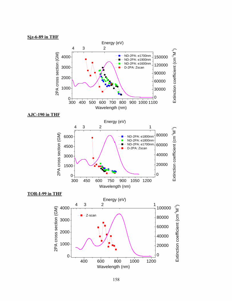
Sjz-6-89 in THF

300 400 500 600 700 800 900 1000 11000

1000

2000

3000

4000 ND-2PA: e1700nm ND-2PA: e1900nm ND-2PA: e1600nm D-2PA: Zscan

2PA

cro

ss s

ectio

n (G

M)

Wavelength (nm)

0

30000

60000

90000

120000

150000

Extin

ctio

n co

effic

ient

(cm

-1M

-1)4 3 2

Energy (eV)

AJC-190 in THF

300 450 600 750 900 1050 12000

1500

3000

4500

6000

2PA

cros

s se

ctio

n (G

M)

Wavelength (nm)


0

20000

40000

60000

80000

Ext

inct

ion

coef

ficie

nt (c

m-1M

-1)4 3 2 1

Energy (eV)

TOR-I-99 in THF

400 600 800 1000 12000

1000

2000

3000

4000

2PA

cro

ss s

ectio

n (G

M)

Wavelength (nm)

Z-scan

0

20000

40000

60000

80000

100000

Ext

inct

ion

coef

ficie

nt (c

m-1M

-1)4 3 2 1

Energy (eV)

158

C.2 NI-COMPLEX FOR 2PA AT TELECOMMUNICATIONS WAVELENTHS [84]


MB-123 JYC-IV-087c

JYC-V-019a

MB-123 in CH2CL2

400 600 800 1000 12000

100

200

300

400

500

2PA

cro

ss s

ectio

n (G

M)

Wavelength (nm)

Z-scan

0

10000

20000

30000

40000

Ext

inct

ion

Coe

ffici

ent (

cm-1M

-1)4 3 2 1

Energy (eV)

159

JYC-IV-087c in CHCL3

400 600 800 1000 1200 14000

500

1000

1500

20002P

A c

ross

sec

tion

(GM

)

Wavelength (nm)

Z-scan

0

10000

20000

30000

40000

50000

60000

Ext

inct

ion

coef

ficie

nt (c

m-1M

-1)4 3 2 1

Energy (eV)

JYC-V-019a in THF

300 450 600 750 900 1050 1200 13500

1500

3000

4500

6000

2PA

cro

ss s

ectio

n (G

M)

Wavelength (nm)

Zscan

0

25000

50000

75000

100000

125000

150000

Ext

inct

ion

coef

feci

ent (

cm-1M

-1)

4 3 2 1Energy (eV)

160

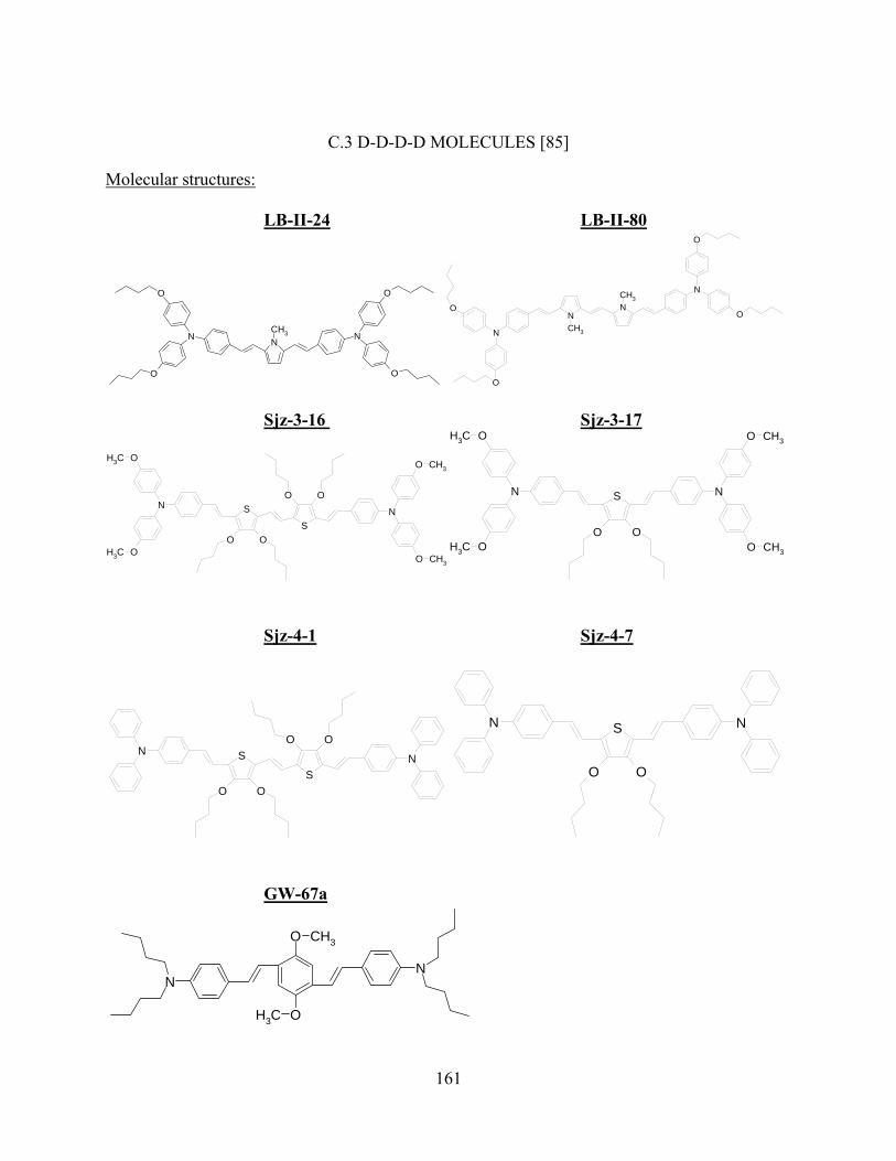
C.3 D-D-D-D MOLECULES [85] Molecular structures:

LB-II-24 LB-II-80

N

O

O

NCH3 N

O

O

NNCH3

CH3N

O

O

N

O

O

Sjz-3-16 Sjz-3-17

S

OS

OO

N

O CH3

O CH

N

O

OCH3

CH3

O

3

N

O CH3

O CH3

S

O

N

O

OCH3

CH3

O

Sjz-4-1 Sjz-4-7

S

OS

OO

NN

O

NS

O

N

O

GW-67a

N

O

O

N

CH3

CH3

161

LB-II-24 in THF

200 300 400 500 6000

1500

3000

4500

6000

7500 ND-2PA: e740nm ND-2PA: e700nm ND-2PA: e660nm Nd-2PA: e620nm D-2PA: Zscan D-2PA: 2PF Q.C. predict

2PA

cro

ss s

ectio

n (G

M)

Wavelength (nm)

0

20000

40000

60000

80000

100000

Extin

ctio

n co

effic

ient

(cm

-1M

-1)

6 5 4 3Energy (eV)

LB-II-80 in THF

300 400 500 600

0

1500

3000

4500

6000 2PF Zscan

2PA

cro

ss s

ectio

n (G

M)

Wavelength (nm)

0

30000

60000

90000

120000

150000

Ext

inct

ion

coef

ficie

nt (c

m-1M

-1)4.5 4 3.5 3 2.5 2

Energy (eV)

Sjz-3-16 in THF

300 400 500 600 7000

1000

2000

3000

4000

5000 2PF Zscan

2PA

cro

ss s

ectio

n (G

M)

Wavelength (nm)

0

30000

60000

90000

120000

Ext

inct

ion

coef

ficie

nt (c

m-1M

-1)

4.5 4 3.5 3 2.5 2Energy (eV)

162

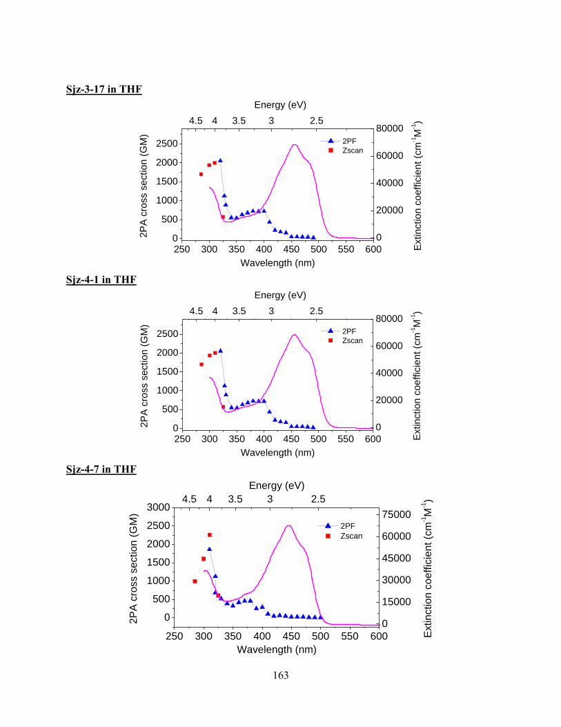
Sjz-3-17 in THF

250 300 350 400 450 500 550 6000

500

1000

1500

2000

25002P

A c

ross

sec

tion

(GM

)

Wavelength (nm)

2PF Zscan

0

20000

40000

60000

80000

Ext

inct

ion

coef

ficie

nt (c

m-1M

-1)4.5 4 3.5 3 2.5

Energy (eV)

Sjz-4-1 in THF

250 300 350 400 450 500 550 6000

500

1000

1500

2000

2500

2PA

cro

ss s

ectio

n (G

M)

Wavelength (nm)

2PF Zscan

0

20000

40000

60000

80000

Ext

inct

ion

coef

ficie

nt (c

m-1M

-1)4.5 4 3.5 3 2.5

Energy (eV)

Sjz-4-7 in THF

250 300 350 400 450 500 550 600

0

500

1000

1500

2000

2500

3000

2PA

cro

ss s

ectio

n (G

M)

Wavelength (nm)

2PF Zscan

0

15000

30000

45000

60000

75000

Ext

inct

ion

coef

ficie

nt (c

m-1M

-1)4.5 4 3.5 3 2.5

Energy (eV)

163

GW-67a in THF

250 300 350 400 450 500 5500

300

600

900

1200

15002P

A c

ross

sec

tion

(GM

)

Wavelength (nm)

2PF Zscan

0

15000

30000

45000

60000

75000

Extin

ctio

n C

oeffe

cien

t (cm

-1M

-1)

4.5 4 3.5 3 2.5

Energy (eV)

164

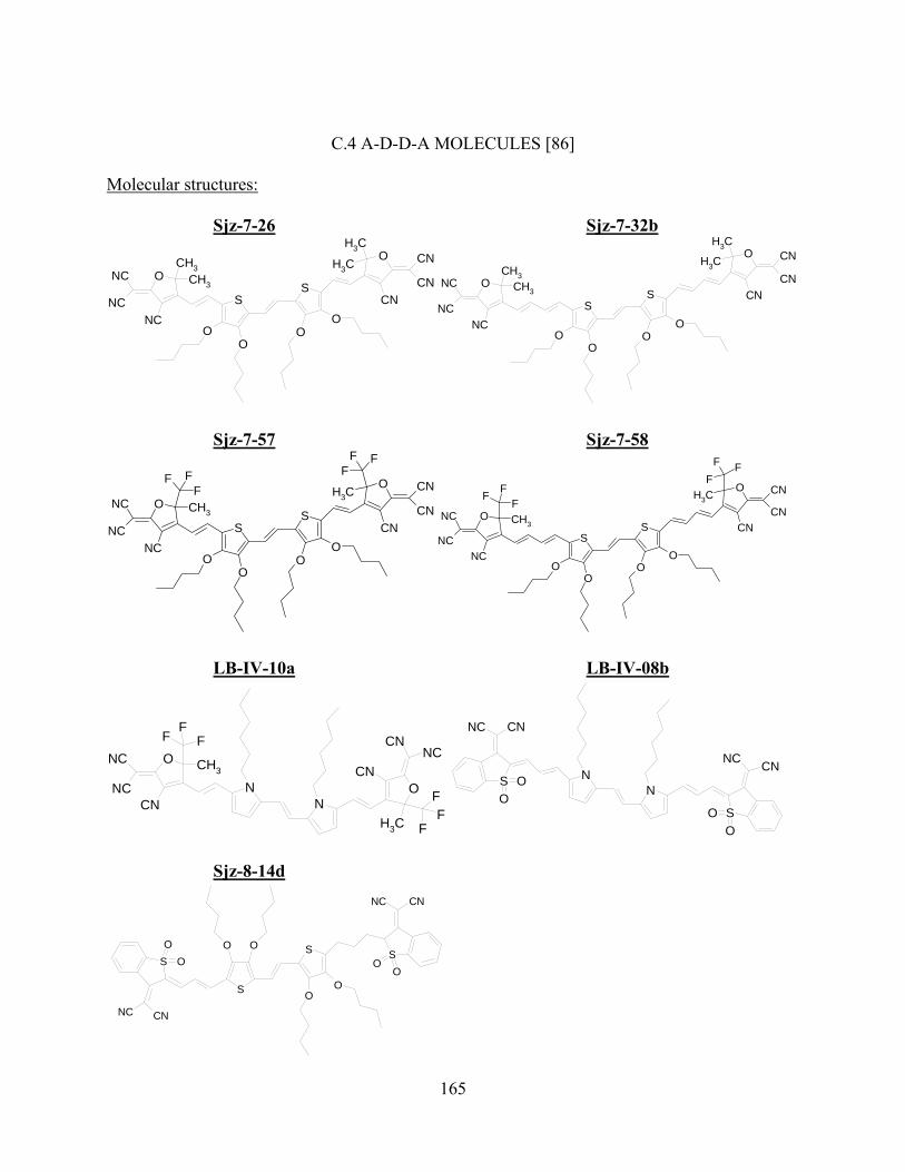
C.4 A-D-D-A MOLECULES [86] Molecular structures:

Sjz-7-26 Sjz-7-32b

SS

OO

OO

OCH3

CH3

CN

CN

CNOCH3

CH3NC

NCNC

OCH3

CH3

CN

CN

CNOCH3

CH3NC

NCNC

SS

OO

OO

Sjz-7-57 Sjz-7-58

SS

OO

OO

OCH3

CN

CN

CNO CH3NC

NCNC

F FF

FFF

OCH3

CN

CN

CNO CH3NC

NCNC

SS

OO

OO

F FF

FFF

LB-IV-10a LB-IV-08b

NN

O

CH3

CNNC

CNO CH3

NC

NC

FF

F

FF

F

CN

NN

SO

O

CNNC

SO

O

CNNC

Sjz-8-14d

S

SO O

OO

S

NC CN

S

NC CN

OO

OO

165

Sjz-7-26 in THF

300 400 500 600 700 800 900 10000

1000

2000

3000

4000

5000

6000 ND-2PA: e1600nm ND-2PA: e1300nm D-2PA: Zscan

2PA

cros

s se

ctio

n (G

M)

Wavelength (nm)

0

20000

40000

60000

80000

Ext

inct

ion

coef

ficie

nt (c

m-1M

-1)4 3 2

Energy (eV)

Sjz-7-32b in THF

300 400 500 600 700 800 900 1000 11000

2000

4000

6000

8000

10000


2PA

cro

ss s

ectio

n (G

M)

Wavelength (nm)

0

20000

40000

60000

80000

100000

120000

Ext

inct

ion

coef

ficie

nt (c

m-1M

-1)4 3 2

Energy (eV)

Sjz-7-57 in THF

300 400 500 600 700 800 900 10000

2000

4000

6000


2PA

cro

ss s

ectio

n (G

M)

Wavelength (nm)

0

20000

40000

60000

80000

100000

Ext

inct

ion

coef

ficie

nt (c

m-1M

-1)

4 3 2Energy (eV)

166

Siz-7-58 in THF

300 400 500 600 700 800 900 1000 11000

2000

4000

6000

8000


2PA

cro

ss s

ectio

n (G

M)

Wavelength (nm)

0

30000

60000

90000

120000

Extin

ctio

n co

effic

ient

(cm

-1M

-1)4 3 2

Energy(eV)

LB-IV-10a in THF

300 400 500 600 700 800 900 10000

2000

4000

6000

8000


2PA

cro

ss s

ectio

n (G

M)

Wavelength (nm)

0

5000

10000

15000

20000

25000

Ext

inct

ion

coef

ficie

nt (c

m-1M

-1)4 3 2

Energy (eV)

LB-IV-08b in THF

300 400 500 600 700 800 900 1000 1100

0

2000

4000

6000

8000


2PA

cro

ss s

ectio

n (G

M)

Wavelength (nm)

0

5000

10000

15000

20000

Ext

inct

ion

coef

ficie

nt (c

m-1M

-1)

4 3 2Energy (eV)

167

Sjz-8-14d in THF

300 400 500 600 700 800 900 10000

1500

3000

4500

6000

7500

90002P

A cr

oss

sect

ion

(GM

)

Wavelength (nm)

D-2PA, Zscan ND-2PA, e1800nm ND-2PA, e1700nm

0

20000

40000

60000

80000

100000

Extin

ctio

n co

effic

ient

(cm

-1M

-1)4 3.5 3 2.5 2 1.5

Energy (eV)

168

C.5 PERYLENE DYE


ZA-III-20 ZA-III-28 ZA-III-100

N

N

OO

OO

N

N

N

N

NN

OO

OO

N

N

OO

OO

O

O

ZA-IV-64 ZA-VII-13b

N

N

O O

OC12H25

OC12H25

OC12H25

OOOC12H25

OC12H25

OC12H25

C10H21

C10H21

N

N

OO

OO

B

B

169

ZA-III-20 in CH2CL2

400 500 600 700 800 900 10000

200

400

600

800

1000

1200

2PA

cro

ss s

ectio

n (G

M)

Wavelength (nm)

Zscan

0

20000

40000

60000

80000

Ext

inct

ion

coef

ficie

nt (c

m-1M

-1)3.5 3 2.5 2 1.5

Energy (eV)

ZA-III-28 in CH2CL2

400 500 600 700 8000

50010001500200025003000

2PA

cro

ss s

ectio

n (G

M)

Wavelength (nm)

Zscan

0

10000

20000

30000

40000

Ext

inct

ion

coef

ficie

nt (c

m-1M

-1)3.5 3 2.5 2 1.5

Energy (eV)

ZA-III-100 in CH2CL2

300 400 500 600 7000

200

400

600

800

1000

2PA

cro

ss s

ectio

n (G

M)

Wavelength (nm)

2PF

0

10000

20000

30000

40000

Ext

inct

ion

coef

ficie

nt (c

m-1M

-1)4 3.5 3 2.5 2

Energy (eV)

170

ZA-IV-64 in CH2CL2

300 400 500 600 7000

300

600

900

12002P

A c

ross

sec

tion

(GM

)

Wavelength (nm)

2PF

0

15000

30000

45000

60000

75000

Ext

inct

ion

coef

ficie

nt (c

m-1M

-1)4.5 4 3.5 3 2.5 2

Energy (eV)

ZA-VII-13b in CH2CL2

300 400 500 6000

4080

120160200240280

2PA

cro

ss s

ectio

n (G

M)

Wavelength (nm)

2PF

0

20000

40000

60000

80000

100000

Ext

inct

ion

coef

ficie

nt (c

m-1M

-1)4.5 4 3.5 3 2.5

Energy (eV)

171

C.6 Naphthalene Derivatives

Molecular Structures: GJW-DAN GJW-1-26a GJW-1-17b

N

N

NH

NH

NH2

NH2

GJW-1-36a GJW-1-48b

N

N

NH

NH

GJW-DAN

250 300 350 400 45002468

101214

2PF

2PA

cro

ss s

ectio

n (G

M)

Wavelength (nm)

0

3000

6000

9000

12000

Ext

inct

ion

coef

ficie

nt (c

m-1M

-1)5.5 5 4.5 4 3.5 3

Energy (eV)

172

GJW-1-26a

250 300 350 400 4500

5

10

15

20

2PA

cro

ss s

ectio

n (G

M)

Wavelength (nm)

2PF

0

5000

10000

15000

Ext

inct

ion

coef

ficie

nt (c

m-1M

-1)5.5 5 4.5 4 3.5 3

Energy (eV)

GJW-1-17b

250 300 350 400 4500

2

4

6

8

10

12

2PA

cro

ss s

ectio

n (G

M)

Wavelength (nm)

2PF

0

3000

6000

9000

12000

Ext

inct

ion

coef

ficie

nt (c

m-1M

-1)5.5 5 4.5 4 3.5 3

Energy (eV)

GJW-1-36a

250 300 350 400 4500

5

10

15

20

25

30

2PA

cro

ss s

ectio

n (G

M)

Wavelength (nm)

2PF

0

10000

20000

30000

40000

Ext

inct

ion

coef

ficie

nt (c

m-1M

-1)5.5 5 4.5 4 3.5 3

Energy (eV)

GJW-1-48a

173

250 300 350 400 4500

5

10

15

20

25

30

2PA

cro

ss s

ectio

n (G

M)

Wavelength (nm)

2PF

0

10000

20000

30000

Ext

inct

ion

coef

ficie

nt (c

m-1M

-1)5.5 5 4.5 4 3.5 3

Energy (eV)

174

C.7 OTHERS


Sjz-3-42 Sjz-6-85

OB

O O OB

FF FF

N NH+

OC10H21

N

N

O OB

FFO O

BFF

OC10H21

+

SC-IV-25c SC-V-10

N

N

N

N

OC12H25

OC12H25

OCH3

OCH3

N

OC6H13

OCH3

O

OC6H13

N

**

n

C6H13

C6H13

XZ-III-28d

Si N

N

175

Sjz-3-42 in CH2CL2

400 500 600 700 800 900 10000

150

300

450

600

750


2PA

cro

ss s

ectio

n (G

M)

Wavelength (nm)

0

50000

100000

150000

200000

250000

300000

Ext

inct

ion

coef

ficie

nt (c

m-1M

-1)3.5 3 2.5 2 1.5

Energy (eV)

Sjz-6-85 in Acetonitrile

300 400 500 600 700 800 900 1000 11000

1000200030004000500060007000

2PA

cro

ss s

ectio

n (G

M)

Wavelength (nm)

ND-2PA: e1900nm ND-2PA: e1400nm ND-2PA; e2000nm ND-2PA: e1330nm D-2PA: Zscan

0

30000

60000

90000

120000

150000

Ext

inct

ion

coef

ficie

nt (c

m-1M

-1)4 3 2

Energy (eV)

SC-IV-25c in CHCL3

250 300 350 400 450 500 550 6000

500

1000

1500

2000

2PF

2PA

cro

ss s

ectio

n (G

M)

Wavelength (nm)

0

30000

60000

90000

120000

150000

180000

Ext

inct

ion

coef

ficie

nt (c

m-1M

-1)4.5 4 3.5 3 2.5

Energy (eV)

176

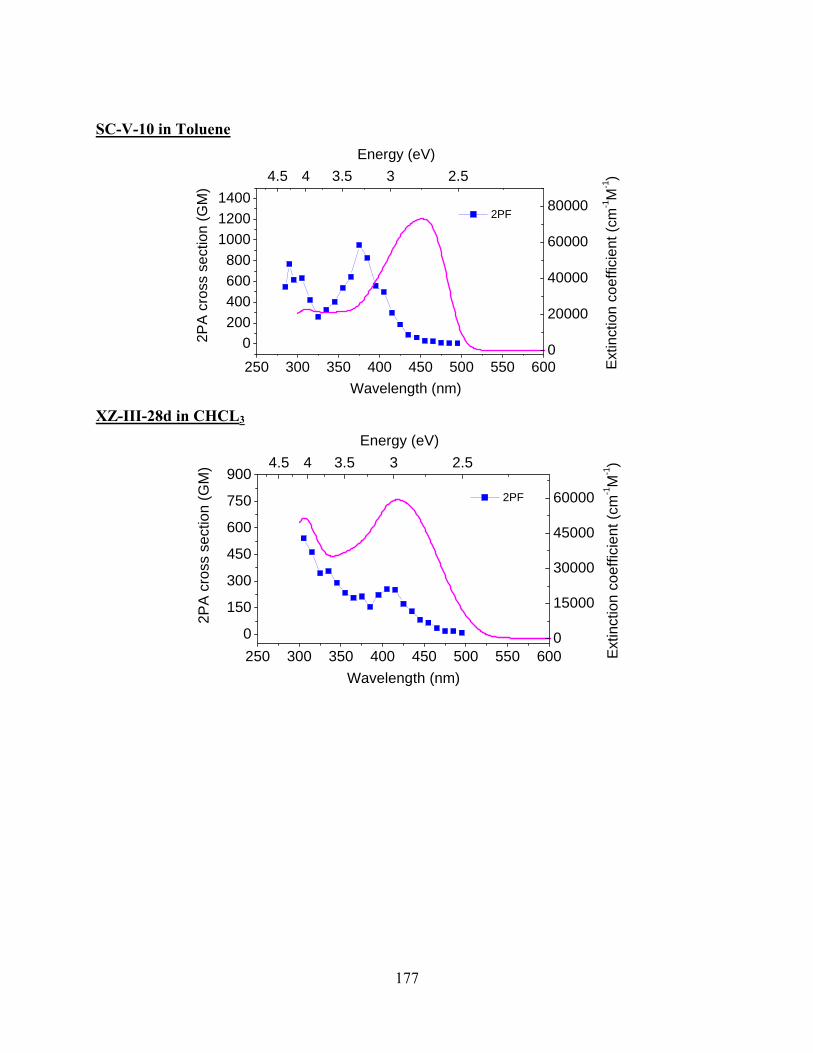
SC-V-10 in Toluene

250 300 350 400 450 500 550 6000

200400600800

100012001400

2PF2P

A c

ross

sec

tion

(GM

)

Wavelength (nm)

0

20000

40000

60000

80000

Ext

inct

ion

coef

ficie

nt (c

m-1M

-1)4.5 4 3.5 3 2.5

Energy (eV)

XZ-III-28d in CHCL3

250 300 350 400 450 500 550 6000

150

300

450

600

750

900 2PF

2PA

cro

ss s

ectio

n (G

M)

Wavelength (nm)

0

15000

30000

45000

60000

Extin

ctio

n co

effic

ient

(cm

-1M

-1)4.5 4 3.5 3 2.5

Energy (eV)

177

APPENDIX D DERIVATIONS FOR TWO-PHOTON EXCITATION FLUORESCENCE

ANISOTROPY

178

The two-photon anisotropy formula derivation is based on two theoretical approaches.

The first is made by P. Callis [79], who used McClain’s original treatment for the two-photon

absorption (2PA) tensor and added the fluorescence transition dipole to develop the equation for

the two-photon anisotropy function. The second theoretical approach is made by P. Cronstrand,

Yi Luo and H. Agren [32]. They derived the equation for the 2PA cross section in a more general

four-state, two-intermediate-level model taking into account the influence of an additional

(second) excitation channel.

Following Callis’ theory, the two-photon anisotropy function, r, is written as

147

718+

−+=

y

yx

QQQ

r (D.1)

where and are functions depending on the 2PA tensor S and fluorescence transition dipole

F. Both Callis and Cronstrand considered only a two-dimensional approximation (case of the

planar molecule oriented in the x-y plane) and linear polarization of the excitation light. For

linear molecules the tensor component S

xQ yQ

zz is much smaller compared to Sxx and Syy, and r depends

only on the and projections. Also, this formula is limited to steady-state conditions with

completely motionless molecules. From [79] it follows that

xQ yQ

(D.2) 22222222 22 yyyyyyxyxxyxxyyxyyxxxxxxx sfsfsfsfsfsfsfsfQ +++++=

(D.3) 2)( yyxxy ssQ +=

where fx, fy and sxx, sxy, syy are normalized matrix elements of S and F.

Substituting Eq.D.2 and D. 3 into Eq. D.1 gives the two-photon anisotropy function, r, as

]2)(

1)(4))(2(9[

72

2

222

2 ++

++−+++=

yyxx

yyxxyyxxyyyxyyxxxxPA ss

sssssfsffsfr (D.4)

179

This is the general formula for steady-state two-photon excitation fluorescence anisotropy,

which is valid for a model including any number of levels. In order to derive an equation for r2PA,

which is possible to apply for analysis of real molecules, we need, first, to choose an adequate

molecular model and, second, to connect the normalized matrix elements fx, fy and sxx, sxy, syy

with the molecular parameters such as transition dipole moments, angles between these

transitions and energy position of the levels.

X

µ01

µ0n

µ1f

µnf

ωh

sn

sf

s1∆E1

∆En

s0

µ1f

µ01

µ0n µnf

µ10ωh

sn

sf

s1∆E1

∆En

s0

µ1f

µ01

µ0n µnf

µ10

f

Y

β

γα

θφ

emβ

01βX

µ01

µ0n

µ1f

µnf

Y

β

γα

θφ

emβ

01β

f

(b) (b)

Figure D.1 Four-state, two-intermediate level (S1 and Sn ) model for two-photon anisotropy, (a) energy states S0, S1, Sf and Sn diagram; (b) transition dipole moments schematic

diagram

First, let’s consider a more general four-state-two-intermediate-level model (or two

scenario model) described in [32] and presented in Fig. D.1 (a). As shown in [32], for this model

the two-photon matrix element S may be presented as , where upper indexes (1)

and (2) indicate the first and the second scenarios of 2PA, and α, β

)2()1(αβαβαβ SSS +=

, yx∈ . If the first scenario

involves the transitions S0 → S1 and S1 → Sf (1 is the first intermediate level and f is the final

180

level) and the second scenario involves transitions S0 → Sn and Sn → Sf (n is the second

intermediate level), matrix elements and may be rewritten as )1(αβS )2(

αβS

1

101

1

101)1(

EES

ff

∆+

∆= αββα

αβ

µµµµ (D.5)

n

nfn

n

nfn

EES

∆+

∆= αββα

αβ

µµµµ 00)2( (D.6)

where µα and µβ are the dipole moments of the participating transitions; ωω hh −=∆ 11E ,

ωω hh −=∆ nnE and ω is the frequency of the excitation. Using Eq. D.5 and D.6, we can write

xx, xy and yy components of matrix elements as: αβS

nfx

nx

fxxxx EE

S µµµµ 0

2

101

1

22∆

+∆

= ; nfy

ny

fyyyy EE

S µµµµ 0

2

101

1

22∆

+∆

= (D.7)

2

0

1

101

2

0

1

101

EEEES

nfx

ny

fxy

nfy

nx

fyx

xy ∆+

∆+

∆+

∆=

µµµµµµµµ (D.8)

The next step is to find the normalized matrix elements , , using the normalized

condition

xxs yys xys

∑ ∗=

αβαβαβ

αβαβ

SS

Ss presented in [79].

After normalization

=xxs222 2 xyyyxx

xx

SSS

S

++,

222 2 xyyyxx

yyyy

SSS

Ss

++= and

222 2 xyyyxx

xyxy

SSS

Ss

++= (D.9)

Substituting relation Eq. D.7 and D.8 into Eq. D.9, gives the normalized matrix

elements , , , expressed in terms of molecular parameters, for Eq. (D.4). However, two-

photon anisotropy (Eq. D.4) includes not only the normalized matrix elements of the 2PA tensor

xxs yys xys

181

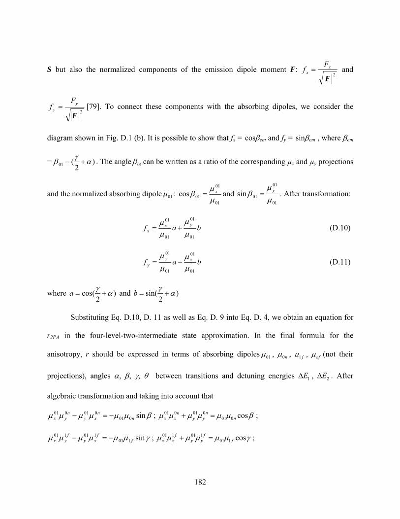
S but also the normalized components of the emission dipole moment F: 2F

xx

Ff = and

2F

yy

Ff = [79]. To connect these components with the absorbing dipoles, we consider the

diagram shown in Fig. D.1 (b). It is possible to show that fx = cosβem and fy = sinβem , where βem

= )2

(01 αγβ +− . The angle can be written as a ratio of the corresponding µ01β x and µy projections

and the normalized absorbing dipole 01µ : 01

01

01cosµµ

β x= and 01

01

01sinµµ

β y= . After transformation:

baf yxx

01

01

01

01

µµ

µµ

+= (D.10)

baf xyy

01

01

01

01

µµ

µµ

−= (D.11)

where )2

cos( αγ+=a and )

2sin( αγ

+=b

Substituting Eq. D.10, D. 11 as well as Eq. D. 9 into Eq. D. 4, we obtain an equation for

r2PA in the four-level-two-intermediate state approximation. In the final formula for the

anisotropy, r should be expressed in terms of absorbing dipoles 01µ , n0µ , f1µ , nfµ (not their

projections), angles α, β, γ, θ between transitions and detuning energies , . After

algebraic transformation and taking into account that

1E∆ 2E∆

βµµµµµµ sin001001001

nn

xyn

yx −=− ; ;

; ;

βµµµµµµ cos001001001

nn

yyn

xx =+

γµµµµµµ sin101101101

ff

xyf

yx −=− γµµµµµµ cos101101101

ff

yyf

xx =+

182

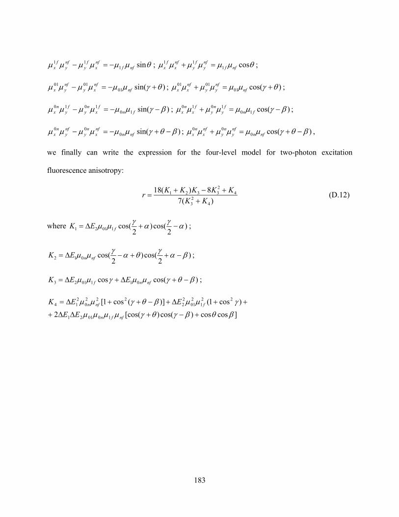
θµµµµµµ sin111

nffnfx

fy

nfy

fx −=− ; ;

; ;

θµµµµµµ cos111

nffnfy

fy

nfx

fx =+

)sin(010101 θγµµµµµµ +−=− nf

nfxy

nfyx )cos(01

0101 θγµµµµµµ +=+ nfnfyy

nfxx

)sin(101010 βγµµµµµµ −−=− fn

fx

ny

fy

nx ; ; )cos(10

1010 βγµµµµµµ −=+ fnf

yn

yf

xn

x

)sin(000 βθγµµµµµµ −+−=− nfn

nfx

ny

nfy

nx ; , )cos(0

00 βθγµµµµµµ −+=+ nfnnfy

ny

nfx

nx

we finally can write the expression for the four-level model for two-photon excitation

fluorescence anisotropy:

)(7

8)(184

23

423321

KKKKKKKr

++−+

= (D.12)

where )2

cos()2

cos(10121 αγαγµµ −+∆= fEK ;

)2

cos()2

cos(012 βαγθαγµµ −++−∆= nfnEK ;

)cos(cos 0110123 βθγµµγµµ −+∆+∆= nfnf EEK ;

]coscos)cos()[cos(2

)cos1()](cos1[

100121

221

201

22

2220

214

βθβγθγµµµµ

γµµβθγµµ

+−+∆∆+

++∆+−++∆=

nffn

fnfn

EE

EEK

183

LIST OF REFERENCES

[1] M. Goppert-Mayer, “Elementary actions with two quantum leaps”, Ann. Physik, Vol. 9, 273

(1931)

[2] W. Kaiser, C.G.B. Garrett, “Two-photon excitation in CaF2:Eu2+”, Phys. Rev. Lett., Vol. 7,

229 (1961)

[3] R. R. Birge and B. M. Pierce, “Semiclassical time-dependent theory of two-photon

spectroscopy. The effect of dephasing in the virtual level on the two-photon excitation

spectrum of isotachysterol”, Int. J. Quan. Chem., Vol. 29, 639 (1986)

[4] W. Denk, J. H. Strickler, and W. W. Webb, “Two-photon laser scanning fluorescence

microscopy”, Science, Vol. 248, 73 (1990)

[5] W. H. Zhou, S. M. Kuebler, K. L. Braun, T. Y. Yu, J. K. Cammack, C. K. Ober, J. W. Perry,

and S. R. Marder, “An efficient two-photon-generated photoacid applied to positive-tone 3D

microfabrication ”, Science, Vol. 296, 1106 (2002)

[6] B. H. Cumpston, S. P. Ananthavel, S. Barlow et al., “Two-photon polymerization initiators

for three-dimensional optical data storage and microfabrication ”, Nature, Vol. 398, 51 (1999)

[7] W. R. Zipfel, R. M. Williams, W. W. Webb, “Nonlinear magic: multiphoton microscopy in

the biosciences”, Nature Biotechnology, Vol. 21, No. 11, 1369 (2003)

[8] A. A. Said, C. Wamsely, D. J. Hagan, E. W. Van Stryland, B. A. Reinhardt, P. Roderer and A.

G. Dillard, “Third- and fifth-order optical nonlinearities in organic materials”, Chem. Phys.

Lett., Vol. 228, 646 (1994)

184

[9] J. D. Bhawalkar, G. S. He and P. N. Prasad, “Nonlinear multiphoton processes in organic and

polymeric materials”, Rep. Prog. Phys., Vol. 59, 1041 (1996)

[10] J. E. Ehrlich, X. L. Wu, Ys. L. Lee, Z. Y. Hu, H. Rockel, S. R. Marder and J. W. Perry,

“Two-photon absorption and broadband optical limiting with bis-donor stilbenes”, Opt. Lett.,

Vol. 22, 1843 (1997)

[11] T. W. Graham Solomons, Organic Chemistry, New York, Wiley, 1996

[12] M. Albota, D. Beljonne, J. Bredas, J. E. Ehrlich, J. Y. Fu, A. A. Heikal, S. E. Hess, T. Kogej,

M. D. Levin, S. R. Marder, D. McCord-Maughon, J. W. Perry, H. Rockel, M. Rumi, G.

Subramaniam, W. W. Webb, X. L. Wu, C. Xu, “Design of organic molecules with large

two-photon absorption cross section”, Science, Vol. 281, 1653 (1998)

[13] M. Rumi, J. E. Ehrlich, A. A. Heikal, J. W. Perry, S. Barlow, Z. Hu, D. McCord-Maughon,

T. C. Parker, H. Rockel, S. Thayumanavan, S. R. Marder, D. Beljonne, and J. Bredas,

“ Structure-property relationships for two-photon absorbing chromophores: bis-donor

diphenylpolyene and bis(styryl)benzene derivatives”, J. Am. Chem. Soc., Vol. 122, 9500

(2000)

[14] K. Ogawa, A. Ohashi, Y. Kobuke, K. Kamada, K. Ohta, “Strong two-photon absorption of

self-assembled butadiyne-linked bisporphyrin”, J. Am. Chem. Soc., Vol. 125, 13356 (2003)

[15] G. P. Bartholomew, M. Rumi, S. J. K. Pond, J. W. Perry, S. Tretiak and G. C. Bazan, “Two-

photon absorption in three-dimensional chromophores based on [2.2]-paracyclophane”, J.

Am. Chem. Soc., Vol. 126, 11529 (2004)

[16] M. Drobizhev, Y. Stepanenko, Y. Dzenis, A. Karotki, A. Rebane, P. N. Taylor and H. L.

Anderson, “Understanding strong two-photon absorption in π-conjugated porphyrin dimers

185

via double-resonance enhancement in a three-level model”, J. Am. Chem. Soc., Vol. 126,

15352 (2004)

[17] S. J. Chung, M. Rumi, V. Alain, S. Barlow, J. W. Perry and S. R. Marder, “Strong, low-

energy two-photon absorption in extened amine-terminated cyano-substituted

phenylenevinylene oligomers”, J. Am. Chem. Soc., Vol. 127, 10844 (2005)

[18] T. K. Ahn, J. H. Kwon, D. Y. Kim, D. W. Cho, D. H. Jeong, S. K. Kim, M. Suzuki, S.

Shimizu, A. Osuka and D. H. Kim, “Comparative photophysics of [26]- and [28]

hexaphyrins(1.1.1.1.1.1): large two-photon absorption cross section of aromatic

[26]hexaphyrins(1.1.1.1.1.1)”, J. Am. Chem. Soc., Vol. 127, 12856 (2005)

[19] L. Beverina, J. Fu, A. Leclercq, E. Zojer, P. Pacher, S. Barlow, E. W. Van Stryland, D. J.

Hagan, J. L. Bredas, and S. R. Marder, “Two-photon absorption at telecommunications

wavelengths in a dipolar chromophore with a pyrrole auxiliary donor and thiazole auxiliary

acceptor”, J. Am. Chem. Soc., Vol. 127, 7282 (2005)

[20] K. D. Belfield, D. J. Hagan, E. W. Van Stryland, K. J. Schafer, R. A. Negres, “New two-

photon absorbing fluorene derivatives: synthesis and nonlinear optical characterization”,

Organic Letters, Vol. 1, No. 10, 1575, (1999)

[21] K. D. Belfield, A. R. Morales, J. M. Hales, D. J. Hagan, E. W. Van Stryland, V. M. Chapela

and J. Percino, “Linear and two-photon photophysical properties of a series of symmetrical

diphenylaminofluorenes”, Chemistry of Materials, Vol. 16, No. 11, 2267 (2004)

[22] E. Zojer, D. Beljonne, T. Kogej, H. Vogel, S. R. Marder, J. W. Perry and J-L. Bredas,

“Tuning the two-photon absorption response of quadrupolar organic molecules”, J. Chem.

Phys., Vol. 116, 3646 (2002)

186

[23] S.R. Marder, “Organic nonlinear optical materials: where we have been and where we are

going”, Chem. Commun. 131-134 (2006).

[24] T. Kogej, D. Beljonne, F. Meyers, J.W. Perry, S.R. Marder, J.L. Bredas, “Mechanisms for

enhancement of two-photon absorption in donor-acceptor conjugated chromophores”, Chem.

Phys. Lett. 298, 1-3 (1998).

[25] G.S. He, T.-C. Lin, J. Dai, P.N. Prasad, R. Kannan, A.G. Dombroskie, R.A. Vaia, L.-S. Tan,

“Degenerate two-photon-absorption spectral studies of highly two-photon active organic

chromophores”, J. Chem. Phys. 120, 5275-5284 (2004).

[26] C.-K. Wang, P. Macak, Yi Luo, H. Agren, “Effects of π centers and symmetry on two-

photon absorption cross sections of organic chromophores”, J. Chem. Phys. 114, 9813-9820

(2001).

[27] D. B, Hochstrasser R. M. and Trommsdorff H. P., Nonlinear optical properties of organic

molecules and crystals, Vol.2, ed D. S. Chemla and J. Zyss, New York: Academic press, pp

167-170 (1987)

[28] J. M. Hales, PhD dissertation, “Chemical structure-nonlinear optical property relationships

for a series of two-photon absorbing fluorene molecules”, 2004

[29] R. W. Boyed, Nonlinear Optics, Academic Press, San Diego (1992)

[30] P. Pacher, “Two-photon absorption in organic molecules”, Diploma thesis, Graz University

of Technology (2003)

[31] B. J. Orr and J. F. Ward, “Perturbation theory of the non-linear optical polarization of an

isolated system”, Mol. Phys., Vol.20, 513 (1971)

[32] P. Cronstrand, Y. Luo and H. Agren, “Generalized few-state models for two-photon

absorption of conjugated molecules”, Chem. Phys. Lett., Vol. 352, 262 (2002)

187

[33] P. R. Monson and W. M. McClain, “Polarization dependence of the two-photon absorption

of tumbling molecules with application to liquid 1-chloronaphthalene and benzene”, J.

Chem. Phys., Vol. 53, No. 1, 29 (1970)

[34] R. R. Birge, J. A. Bennett, B. M. Pierce and T. M. Thomas, “Two-photon spectroscopy of

the visual chromophores. Evidence for a lowest excited 1Ag-_Like ππ* state in all-trans-

retinol (Vitamin A)”, J. Am. Chem. Soc., Vol. 100, No. 5, 1533 (1978)

[35] K. Kamada, K. Ohta, Y. Iwase, K. Kondo, “Two-photon absorption properties of symmetric

substituted diacetylene: drastic enhancement of the cross section near the one-photon

absorption peak”, Chem. Phys. Lett., Vol. 372, 386 (2003)

[36] R. R. Birge, Ultrasensitive Laer Spectrosocopy, Ed. D. S. Kliger, Academic Press: New

York, 109 (1983)

[37] G. Herzberg, Molecular spectra and molecular structure. I. Spectra of diatomic molecules,

Van Nostrand Reinhold Company: New York, 381 (1950)

[38] R. S. Mulliken, “Intensities of electronic transitions in molecular spectra”, J. Chem. Phys.,

Vol.7, 14 (1939)

[39] J. R. Lakowicz, Principle of fluorescence spectroscopy, 2nd edition, Kluwer

Academic/Plenum Publisher: New York, (1999)

[40] M. Fischer, J. Georges, “Fluorescence quantum yield of rhodamine 6G in ethanol as a

function of concentration using thermal lens spectrometry”, Chem. Phys. Lett., Vol. 260,

115 (1996)

[41] M. Sheik-Bahae, A. A. Said, T. Wei, D. J. Hagan, E. W. Van Stryland, “Sensitive

measurement of optical nonlinearities using a single beam”, IEEE J. Quantum. Electron.,

Vol. 26, 760 (1990)

188

[42] C. Xu and W. W. Webb, “Measurement of two-photon excitation cross sections of

molecular fluorophores with data from 690 to 1050nm”, J. Soc. Opt. Am. B, Vol. 13, No. 3,

481 (1996)

[43] W. M. McClain and R. A. Harris, Two-photon molecular spectroscopy in liquids and gases

in excited states, E. C. Lim, ed. Academic, New York, 1 (1977)

[44] R. A. Negres, J. M. Hales, A. Kobyakov, D. J. Hagan, E. W. Van Stryland, “Experiment and

analysis of two-photon absorption spectroscopy using a white-light continuum probe”, IEEE

J. Quantum Electron. Vol. 38, No. 9, 1205 (2002)

[45] R. A. Negres, “Ultrafast nonlinear spectrometer for material characterization”, PhD thesis,

2001

[46] A. Brodeur, S. L. Chin, “Bandgap dependence of the ultrafast white-light continuum”’ phys.

Rev. Lett., Vol. 80, 4406 (1998)

[47] C.H.G. Williams, Trans. R. Soc. Edinburg, 211, 377 (1856)

[48] M. T. Spitler, A. Ehret, R. Kietzmann and F. Willig, “Electron transfer threshold for spectral

sensitization of silver halides by monomeric cyanine dyes”, J. Phys. Chem. B, Vol.101,

2552 (1997)

[49] N. Tyutyulkov, et. al., Polymethine dyes structure and properties, Sofia, St. Kliment

Ohridski University Press, (1991)

[50] Y. Miyazoe and M. Maeda, “Stimulated emission from 19 polymethine dyes-laser action

over the continuous range 710-1060 nm,” App. Phys. Lett. Vol.12, No.5, 206 (1968)

[51] E. Terpetschnig, H. Szmacinski, A. Ozinskas, J. R. Lakowicz, “Synthesis of squaraine-N-

hydroxysuccinimide esters and their biological application as long-wavelength fluorescent

labels”, Anal. Biochem., Vol. 217, 197 (1994)

189

[52] J. H. Lim, O. V. Przhonska, S. Khodja, S. Yang, T. S. Ross, D. J. Hagan, E. W. Van

Stryland, M. V. Bondar, Y. L . Slominsky, “Polymethine and squarylium molecules with

large excited-state absorption”, Chem. Phys., Vol. 245, 79 (1999)

[53] R. S. Lepkowicz, O. V. Przhonska, J. M. Hales, D. J. Hagan, E. W. Van Stryland, M. V.

Bondar, Y. L. Slominsky, A. D. Kachkovski, “Excited-state absorption dynamics in

polymethine dyes detected by polarization-resolved pump-probe measurements”, Chem.

Phys., Vol. 286, 277 (2003)

[54] Y.H. Meyer, M. Pittman, and P. Plaza, “Transient absorption of symmetrical

carbocyanines,” J. Photochem. Photobiol. A, Vol. 114, 1, 1998

[55] R. S. Lepkowicz, Olga V. Przhonska, J. M. Hales, J. Fu, David J. Hagan, E. W. Van

Stryland, M. V. Bondar, Y. L. Slominsky, A. D. Kachkovski, “Nature of the electronic

transitions in thiacarbocyanines with a long polymethine chain”, Chem. Phys. Vol. 305,

p259 (2004)

[56] J. M. Hales, D. J. Hagan, E. W. Van Stryland, K. J. Schafer, A. R. Morales, K. D. Belfield,

P. Pacher, O. Kwon, E. Zojer, J. L. Bredas “Resonant enhancement of two-photon absorption

in substituted fluorene molecules”, J. Chem. Phys., Vol. 121 (7), 3125, 2004

[57] W. M. McClain, “Excited state symmetry assignment through polarized two-photon

absorption studies of fluids”, J. Chem. Phys., Vol. 55, 2789-2796 (1971)

[58] D. M. Friedrich and W. M. McClain, “Two-photon molecular electronic spectroscopy”,

Annu. Rev. Phys. Chem., Vol. 31, 559-577 (1980)

[59] M.J.S. Dewar, The molecular orbital theory of organic chemistry (McGrow-Hill, New York,

1969)

190

[60] D. Scherer, R. Dorfler, A. Feldner, T. Vogtmann, M. Schwoerer, U. Lawrentz, W. Grahn

and C. Lambert, “Two-photon states in squaraine monomers and oligomers”, Chem. Phys.,

Vol. 279, 179 (2002)

[61] P. R. Callis, T. W. Scott and A. C. Albrecht, “Perturbation selection rules for multiphoton

electronic spectroscopy of neutral alternant hydrocarbons”, J. Chem. Phys., Vol. 78, 16 (1983)

[62] T. W. Scott, P. R. Callis and A. C. Albrecht, “Alternant hydrocarbon selection rules in the

two-photon spectroscopy of perturbed benzenes”, Chem. Phys. Lett., Vol. 93, 111 (1992)

[63] J. Fu, O.V. Przhonska, L.A. Padilha, D.J. Hagan, E.W. Van Stryland, K.D. Belfield, M.V.

Bondar, Yu.L. Slominsky, A.D. Kachkovski, “Two-photon anisotropy: Analytical

description and molecular modeling for symmetrical and asymmetrical organic dyes”, Chem.

Phys., Vol. 321, 257 (2006)

[64] M. Hamer, The Cyanine Dyes and Related Compounds, Interscience Publisher, New York,

1964

[65] J.S. Craw, J.R. Reimers, G.B. Bacskay, A.T. Wong, N.S. Hush, “Solitons in finite- and

infinite-length negative-defect trans-polyacetylene and the corresponding Brooker

(polymethinecyanine) cations”, Chem. Phys. Vol. 167, 77 (1992)

[66] S. J. Chung, S. J. Zheng, T. Odani, L. Beverina, J. Fu, L. A. Padilha, A. Biesso, J. M. Hales,

X. W. Zhan, K. Schmidt, A. J. Ye, E. Zojer, S. Barlow, D. J. Hagan, E. W. Van Stryland, Y.

P. Yi, Z. G. Shuai, G. A. Pagani, J-L. Bredas, J. W. Perry and S. R. Marder, “Extended

squaraine dyes with large two-photon absorption cross sections”, submitted to J. Am. Chem.

Soc.

191

[67] Dewar, M. J. S.; Zoebisch, E. G.; Healy, E. F.; Stewart, J. J. P., “Development and use of

quantum mechanical molecular models. 76. AM1: a new general purpose quantum

mechanical molecular model”, J. Am. Chem. Soc. Vol. 107, 3902 (1985)

[68] Ridley, J.; Zerner, M., “An intermediate neglect of differential overlap technique for

spectroscopy: Pyrrole and the azines” Theo. Chem. Acta Vol. 32, 111 (1973)

[69] Mataga, N.; Nishimoto, K., Z. “ ”, Phys. Chem. Vol. 13, 140 (1957)

[70] Purvis, G. D.; Bartlett, R. J., “A full coupled-cluster singles and doubles model: The

inclusion of disconnected triples” J. Chem. Phys. Vol. 76, 1910 (1982)

[71] Shuai, Z.; Brédas, J. L., “Coupled-cluster approach for studying the electronic and nonlinear

optical properties of conjugated molecules” Phys. Rev. B. Vol. 62, 15452 (2000)

[72] Buenker, R. J.; Peyerimhoff, S. D., “Individualized configuration selection in CI

calculations with subsequent energy extrapolation” Theo. Chem. Acta ,Vol. 35, 33 (1974)

[73] Tavan, P.; Schulten, K., “The low-lying electronic excitations in long polyenes: A PPP-

MRD-CI study” J. Chem. Phys. Vol. 85, 6602 (1986)

[74] Guo, D.; Mazumdar, S.; Dixit, S. N.; Kajzar, F.; Jarka, F.; Kawabe, Y.; Peyghambarian, N.,

“Role of the conduction band in electroabsorption, two-photon absorption, and third-

harmonic generation in polydiacetylenes” Phys. Rev. B Vol. 48, 1433 (1993)

[75] Heflin, J. R.; Wong, K. Y.; Zamani-Khamiri, O.; Garito, A. F., “Nonlinear optical properties

of linear chains and electron-correlation effects” Phys. Rev. B Vol. 38, 1573 (1988)

[76] Tavan, P.; Schulten, K., “Electronic excitations in finite and infinite polyenes” Phys. Rev. B

1987, 36, 4337

192

http://www.springerlink.com/(wdu3t1eaefa330voj0wwfd55)/app/home/contribution.asp?referrer=parent&backto=issue,3,10;journal,388,540;linkingpublicationresults,1:100493,1

http://www.springerlink.com/(wdu3t1eaefa330voj0wwfd55)/app/home/contribution.asp?referrer=parent&backto=issue,3,10;journal,388,540;linkingpublicationresults,1:100493,1

[77] Shuai, Z.; Beljonne, D.; Brédas, J. L., “Nonlinear optical processes in short polyenes:

Configuration interaction description of two-photon absorption and third-harmonic

generation” J. Chem. Phys. Vol. 97, 1132 (1992)

[78] Zojer, E.; Beljonne, D.; Pacher, P.; Brédas, J. L., Chem. Eur. J. Vol.10, 2668 (2004)

[79] P.R. Callis, in: J.R. Lakowicz (Ed.) Topics in fluorescence spectroscopy, V. 5, Plenum Press,

New York – London, p1. (1997)

[80] K. D. Belfield, M. V. Bondar, J. M. Hales, A. R. Morales, O. V. Przhonska, K. J. Schafer,

“One- and two-photon fluorescence anisotropy of selected fluorene derivatives” J. Fluoresc.

Vol. 15, No. 1, 3 (2005)

[81] J.R. Lakowicz, I. Gryczynski, in J.R. Lakowicz (Ed.), Topics in fluorescence spectroscopy,

V. 5, Plenum Press, New York – London, p87 (1997)

[82] V. Gaisenok, A. Sarzhevskii, Absorption and fluorescence anisotropy of complicated

molecules, University Press, Minsk, (1986)

[83] L. Beverina, J. Fu, A. Leclercq, E. Zojer, P. Pacher, S. Barlow, E. W. Van Stryland, D. J.

Hagan, J-L. Bredas, S. R. Marder, “Two-photon absorption at telecommunications

wavelengths in a dipolar chromophore with a pyrrole auxiliary donor and thiazole auxiliary

acceptor”, J. Am. Chem. Soc., Vol. 127, 7282 (2005)

[84] J. Y. Cho, S. Barlow, S. R. Marder, J. Fu, L. A. Padilha, E. W. Van Stryland, D. J. Hagan,

M. Bishop, “Strong two-photon absorption at telecommunications wavelengths in nickel

dithiolene complexes”, submitted to Optics Letters

[85] S. J. Zheng, L. Beverina, J. Fu, L. A. Padilha, E. Zojer, S. Barlow, C. Fink, O. Kwon, Y. P.

Yu, E. W. Van Stryland, D. J. Hagan, J-L. Bredas and S. R. Marder. “High two-photon

193

cross-sections in bis(diaryaminostyryl) chromophores with electron-rich heterocycle and

bis(heterocycle)vinylene bridges”, submitted to

[86] S. J. Zheng, A. Leclercq, J. Fu, L. Beverina, L. A. Padilha, E. Zojer, K. Schmidt, S. Barlow,

J. D. Luo, S. H. Jiang, A. Jen, Y. P. Yi, Z. G. Shuai, E. W. Van Stryland, D. J. Hagan, J-L

Bredas and S. R. Marder, “Two-photon absorption in quadrupolar bis(acceptor)-terminated

chromophores with electron-rich bis(heterocycle)viny bridges”, submitted to Chemical

Material

194

Molecular Structure-nonlinear Optical Property ...

Documents

Transcript of Molecular Structure-nonlinear Optical Property ...