Molecular Interactions - University of Manchester

Chapter 3Molecular Interactions

Contents3.1 Introduction . . . . . . . . . . . . . . . . . . . . . . . . . . . . . . . 47

3.2 Molecular Force Fields . . . . . . . . . . . . . . . . . . . . . . . . . 47

3.2.1 Stretching energy . . . . . . . . . . . . . . . . . . . . . . . . . 48

3.2.2 Bending Energy . . . . . . . . . . . . . . . . . . . . . . . . . 48

3.2.3 Torsional Energy . . . . . . . . . . . . . . . . . . . . . . . . . 49

3.2.4 Van der Waals . . . . . . . . . . . . . . . . . . . . . . . . . . 50

3.2.5 Electrostatic Energy . . . . . . . . . . . . . . . . . . . . . . . 52

3.2.6 Cross Terms . . . . . . . . . . . . . . . . . . . . . . . . . . . 52

3.3 Choice of Force Field . . . . . . . . . . . . . . . . . . . . . . . . . . 53

3.3.1 Universal Force Field (UFF) . . . . . . . . . . . . . . . . . . . 53

3.3.2 Assisted Model Building with Energy Refinement (AMBER) . . 53

3.3.3 Chemistry at HARvard Molecular Mechanics (CHARMM) . . . 54

3.3.4 Optimised Potentials for Liquid Simulations (OPLS) . . . . . . 54

3.3.5 GROningen MOlecular Simulation (GROMOS) . . . . . . . . . 54

3.3.6 Transferable Potentials for Phase Equilibria (TraPPE) . . . . . . 54

3.4 Water Models . . . . . . . . . . . . . . . . . . . . . . . . . . . . . . 55

3.4.1 Explicit Water . . . . . . . . . . . . . . . . . . . . . . . . . . 55

3.4.2 Implicit Water . . . . . . . . . . . . . . . . . . . . . . . . . . 56

3.5 Coarse-Graining . . . . . . . . . . . . . . . . . . . . . . . . . . . . . 59

3.5.1 Mapping . . . . . . . . . . . . . . . . . . . . . . . . . . . . . 60

3.5.2 Potentials . . . . . . . . . . . . . . . . . . . . . . . . . . . . . 60

3.5.3 Iterative Boltzmann Inversion . . . . . . . . . . . . . . . . . . 60

3.6 References . . . . . . . . . . . . . . . . . . . . . . . . . . . . . . . . 61

45

3.1. INTRODUCTION 47

3.1 IntroductionWhen molecules are near each other, they can influence one another. Therefore, the bal-ance between the forces of attraction and repulsion needs to be understood. Such forcesmust exist in reality otherwise there would be nothing to bring molecules together to formliquid and solid states. People have speculated about these intermolecular forces since theconcept of atoms and molecules first existed. The present theory is that molecules attractat long range but repel strongly at short range.

3.2 Molecular Force FieldsActual interactions between atoms is in the realm of physical chemistry. For computa-tional simulations, these interactions are too complex to simulate systems larger than acouple of molecules on the current computers available. Therefore, it is common practiseto represent these real interactions as a computational force field. The choice of compu-tational method is dependent on the size of the system and the time scales of calculations.For systems with up to several hundred to several thousand atoms, the molecules can berepresented as individual atoms with each atom represented by a sphere. There are manytypes of force field, but they all follow a similar pattern:

• Nuclei and electrons are combined in an atom, represented by a ball.

• A ball has a radius and a constant charge. The ball can vary in softness.

• Bonds are represented by springs.

• Springs have an equilibrium length and can vary in stiffness.

The interactions between these spheres form the molecular force field. The interac-tions are described by pre-assigned parameters, that are system dependent. These param-eters can be obtained from experiment and/or higher level computational calculations,such as ab-initio. The force field is the set of parameters used in classical mechanicalcalculations. The potential energy of the system is described by the sum of all the interac-tions within the system, equation 3.2.1, where Estr is the energy function for stretching abond between two atoms, Ebend is the energy required for bending an angle between threeatoms, Etors is the torsional energy for rotation around a bond, EV dW is the Van der Waalsenergy, Eel is the electrostatic energy, and EXterms represents any coupling between theabove terms.

EFF = Estr + Ebend + Etors + EV dW + Eel + EXterms (3.2.1)

The first three terms represent the bonded interactions. The electrostatic and Van derWaals energies are non bonded interactions between atoms. To be able to calculate theforce field energy it is necessary to know atomic coordinates, geometries, and the relativeenergies of the atoms in the system.

The calculation of the total potential energy is dominated by the number of non-bonded interactions. The time for calculation of the bonded interactions increase on theorder of ∼ N , while the time for calculation of the non-bonded interactions increase onthe order of ∼ N2.

48 CHAPTER 3. MOLECULAR INTERACTIONS

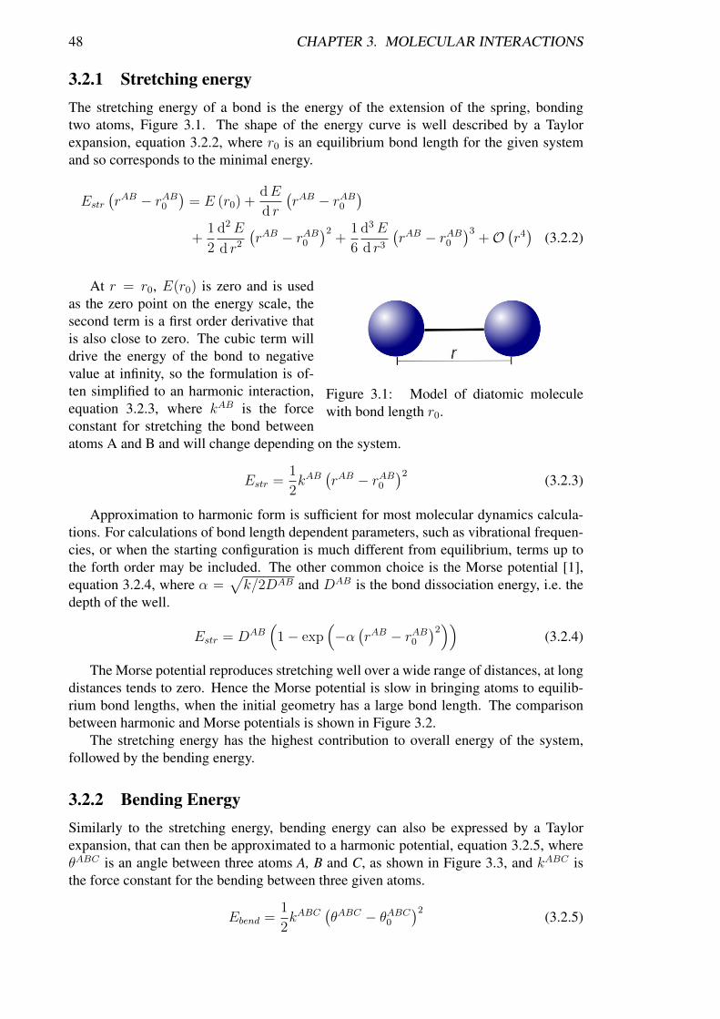
3.2.1 Stretching energyThe stretching energy of a bond is the energy of the extension of the spring, bondingtwo atoms, Figure 3.1. The shape of the energy curve is well described by a Taylorexpansion, equation 3.2.2, where r0 is an equilibrium bond length for the given systemand so corresponds to the minimal energy.

Estr(rAB − rAB0

)= E (r0) +

dE

d r

(rAB − rAB0

)+

1

2

d2E

d r2

(rAB − rAB0

)2+

1

6

d3E

d r3

(rAB − rAB0

)3+O

(r4)

(3.2.2)

Figure 3.1: Model of diatomic moleculewith bond length r0.

At r = r0, E(r0) is zero and is usedas the zero point on the energy scale, thesecond term is a first order derivative thatis also close to zero. The cubic term willdrive the energy of the bond to negativevalue at infinity, so the formulation is of-ten simplified to an harmonic interaction,equation 3.2.3, where kAB is the forceconstant for stretching the bond betweenatoms A and B and will change depending on the system.

Estr =1

2kAB

(rAB − rAB0

)2(3.2.3)

Approximation to harmonic form is sufficient for most molecular dynamics calcula-tions. For calculations of bond length dependent parameters, such as vibrational frequen-cies, or when the starting configuration is much different from equilibrium, terms up tothe forth order may be included. The other common choice is the Morse potential [1],equation 3.2.4, where α =

√k/2DAB and DAB is the bond dissociation energy, i.e. the

depth of the well.

Estr = DAB(

1− exp(−α(rAB − rAB0

)2))

(3.2.4)

The Morse potential reproduces stretching well over a wide range of distances, at longdistances tends to zero. Hence the Morse potential is slow in bringing atoms to equilib-rium bond lengths, when the initial geometry has a large bond length. The comparisonbetween harmonic and Morse potentials is shown in Figure 3.2.

The stretching energy has the highest contribution to overall energy of the system,followed by the bending energy.

3.2.2 Bending EnergySimilarly to the stretching energy, bending energy can also be expressed by a Taylorexpansion, that can then be approximated to a harmonic potential, equation 3.2.5, whereθABC is an angle between three atoms A, B and C, as shown in Figure 3.3, and kABC isthe force constant for the bending between three given atoms.

Ebend =1

2kABC

(θABC − θABC0

)2(3.2.5)

3.2. MOLECULAR FORCE FIELDS 49

Figure 3.2: Bond stretching energy. Harmonic potential compared to the Morse potential.

Figure 3.3: An angle between three bondedatoms.

When a higher accuracy is required forthe calculation, the next highest order termin the expansion can be included, or a se-ries of harmonic potentials can be used.

Changes in the bending energy are usu-ally smaller than the changes in stretch-ing energy, so less energy is required todistort bond angles in comparison to bondlength. Hence, force constants for bend-ing are proportionally smaller than thosefor stretching.

Figure 3.4: An illustration of out-of-planebending, created by three atoms bonded tosp2 hybridised central atom.

When the central atom B is bondedto more than two other atoms, as shownon the Figure 3.4, a pyramidal structure isformed. This angle can no longer be cal-culated in the manner discussed above. Ahigh force constant should be used to pe-nalise out-of-plane bending, this will makeplanar structures very inflexible. By intro-ducing a new term, the flexibility of theplanar structure is maintained while out-of-plane movement is also taken into ac-count. This bending is often referred to asthe improper torsional energy. This also

often takes the form of a harmonic potential, equation 3.2.6.

Eimproper =1

2kB(α)2 (3.2.6)

3.2.3 Torsional EnergyFour aligned atoms frequently will rotate along the central bond, as shown in Figure 3.5.

Rotation along the bond is continuous, so when the bond rotates by 360◦ the energyshould return to the initial value, making torsional energy periodic. The potential is well


Figure 3.5: Torsional / dihedral angle, created by four linearly aligned atoms.

represented by the Fourier series, equation 3.2.7, where n is a periodicity term, dependingon the allowed rotation it can be n = 1 for full 360◦ rotation, n = 2 for 180◦ periodicity,n = 3 for 120◦ periodicity, etc. Vn is a constant determining the barrier for the rotation,Vn is not equal to zero for allowed periodic rotations, ϕ is the torsional angle (also calledthe dihedral angle) and is shown on the Figure 3.5.

Etors =∑n

Vn cos (nϕ− ϕ0) (3.2.7)

Figure 3.6 shows a plot of the two torsional potentials with n = 3, Vn = 4 (dashedline), n = 2, Vn = 3 (solid line) and the corresponding total torsional potential in red ifthe two are combined.

Figure 3.6: Variation of torsional potential for different values of n and Vn and the totalpotential (red).

3.2.4 Van der WaalsIn addition to the bonded interactions described above, there are non bonded interactionsin the system. These interactions appear between atoms in the same or neighbouringmolecule and are normally described by two potentials, representing the Van der Waalsenergy and the electrostatic energy.

3.2. MOLECULAR FORCE FIELDS 51

The Van der Waals energy describes the repulsion and attraction between non bondedatoms. At large interatomic distances the Van der Waals energy goes to zero, whereas atshort distances it is positive and very repulsive. This mimics the overlap of the negativelycharged electronic clouds of atoms. At intermediate distances there is a mild attractionbetween electronic clouds, due to electron-electron correlation. The attraction betweentwo atoms arises because of an induced dipole–dipole moment created by the motion ofelectrons through the molecule, which effects the neighbouring molecule. The attractionbetween two fragments does not only depend on dipole–dipole interactions, but also ondipole–quadrupole, quadrupole–quadrupole etc. interactions. These interactions do nothave a high contribution to the overall energy, so for simplicity they are neglected incalculations.

In 1903, Gustav Mie proposed an intermolecular pair potential [2], comprising twoparts to represent attractive and repulsive forces, equation 3.2.8, where r is interatomicdistance, ε is the depth of the well at σ, the interatomic separation at which repulsive andattractive terms balance out and m,n can be adjusted.

Epair(r) =

(n

n−m

)( nm

)m/(n−m)

ε[(σr

)n−(σr

)m](3.2.8)

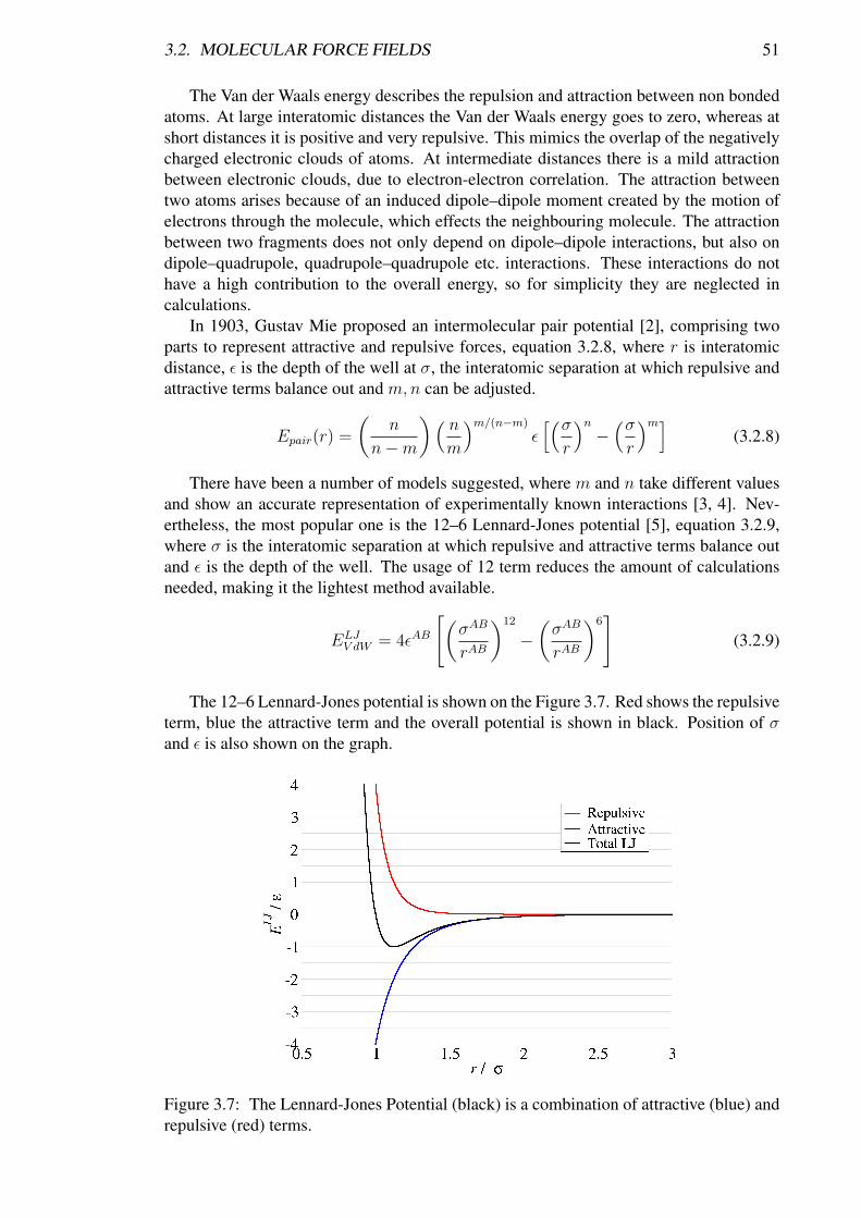
There have been a number of models suggested, where m and n take different valuesand show an accurate representation of experimentally known interactions [3, 4]. Nev-ertheless, the most popular one is the 12–6 Lennard-Jones potential [5], equation 3.2.9,where σ is the interatomic separation at which repulsive and attractive terms balance outand ε is the depth of the well. The usage of 12 term reduces the amount of calculationsneeded, making it the lightest method available.

ELJV dW = 4εAB

[(σAB

rAB

)12

−(σAB

rAB

)6]

(3.2.9)

The 12–6 Lennard-Jones potential is shown on the Figure 3.7. Red shows the repulsiveterm, blue the attractive term and the overall potential is shown in black. Position of σand ε is also shown on the graph.

Figure 3.7: The Lennard-Jones Potential (black) is a combination of attractive (blue) andrepulsive (red) terms.


It is possible to mix two Lennard-Jones potentials for single type atoms to obtaina potential describing interaction between two different atoms. There are three mainapproaches:

• Arithmetic or Lorentz-Berthelot rules, equations 3.2.10 and 3.2.11 [6].

σij =σii + σjj

2(3.2.10)

εij =√εiiεjj (3.2.11)

• Geometric rules equation 3.2.12, with εij calculated as given in equation 3.2.11 [7].

σij =√σiiσjj (3.2.12)

• Fender-Halsey rule, equation 3.2.13 [8].

εij =2εiεjεi + εj

(3.2.13)

A slightly more accurate potential, but up to 4 times more computationally demand-ing, is the Buckingham or Hill potential [4]. Repulsive forces take the form of an ex-ponential, as the repulsion arises due to electron correlation, and the electron densityreduces exponentially with the distance, equation 3.2.14, where A,B, and C are suitableconstants.

EHillV dW = A exp (−BrAB)− Cr6

AB (3.2.14)

3.2.5 Electrostatic EnergyThe electrostatic energy calculates non bonded interactions that appear due to an uneveninternal distribution of electrons. This leads to positively and negatively charged parts inmolecule. The simplest way to model this behaviour is to place charges on atoms. Thelaw of the interaction between two point charges was investigated by Charles AugustinCoulomb in 1780s and can be expressed by the Coulomb potential, equation 3.2.15, whereε0 is the dielectric constant, the Q values are partial electronic charges on atoms A and B,and r is a distance between them.

Eel =1

4πε0

QAQB

rAB(3.2.15)

The atomic charges are mainly taken from electrostatic potential calculations carriedout using higher precision methods. Another approach arises from assigning bond dipolemoments. This gives similar results to the partial charge method, but these two methodswill only give identical results for interactions at larger distances.

3.2.6 Cross TermsThere are also cross terms available for some force fields. These can cover the couplingbetween the fundamental stretching, bending and torsional interactions.

3.3. CHOICE OF FORCE FIELD 53

3.3 Choice of Force FieldThe correct choice of the force field is essential for performing an accurate simulation. Alarge number of force fields have been developed through last decades. The force fieldconsists of a set of parameters that depend on a particular the atom and the interaction.

Ideally force fields are designed to be transferable between a number of molecular sys-tems. Nevertheless, some are more suitable for particular systems and states, then others.Comparison of the performance of the force filed should be done with a specific studyin mind. Typical tests include the comparison to the experimental physical properties,such as density, boiling and melting temperatures, secondary protein structure, as wellas the agreement with vapour-liquid coexistence, and the reproduction of thermodynamicproperties.

Most force fields represent all atom systems, with a few being united atom wherehydrogens are united to the neighbouring heavy atoms. United atom representation hasless interactions, by such speeding up the calculations. Not every system can be accuratelyrepresented as united atom, for example systems having hydrogen bonding, benzene rings,polar and charged systems.

All atom force fields:

• OPLS-AA(Optimised Potentials for Liquid Simulations) [9]

• CHARMM (Chemistry at HARvard Macromolecular Mechanics) [10]

• AMBER (Assisted Model Building with Energy Refinement) [11]

• UFF (Universal Force Field) [12]

United atom force fields:

• OPLS (Optimised Potentials for Liquid Simulations)[13]

• CHARMM (Chemistry at HARvard Macromolecular Mechanics) [10]

• GROMOS (GROningen MOlecular Simulation) [14]

• TraPPE (Transferable Potentials for Phase Equilibria) [15]

3.3.1 Universal Force Field (UFF)UFF [12] was developed by Rappe et. al. in 1992. It is an unusual force field, unlikeothers it covers the full periodic table, from hydrogen to lawrencium. The parameters areobtained by estimating from given general rules, that convert individual parameters forthe element into the intermolecular and intramolecular parameters for calculations.

The performance of this force field with respect to the experimental results [16], is notvery consistency, so it is not really suitable for high accuracy condensed state calculations.This force field is however useful for calculations of exotic molecules, where other forcefield have not been created.

3.3.2 Assisted Model Building with Energy Refinement (AMBER)AMBER is both a molecular dynamics package and a set of force fields [11, 17]. The forcefield uses 12-6 Lennard-Jones, equation 3.2.9, with parameters computed by Lorentz-Berthelot mixing rules, equations 3.2.10 and 3.2.11, 1-4 interactions are scaled by 1

2and


Columbic interactions are represented by point charges and are scaled by 56. Bond and

angle interactions are expressed as harmonic potentials and torsional interactions are rep-resented as a cosine series.

AMBER force fields are all atom only (though the newest force field, ff12sb, does in-clude some united atom parameter), parametrised for biomolecular simulations and con-tains the 20 common amino acids as functional groups. More recently there have beensome work put in to extend the AMBER force field to a wider range of systems throughthe development of the general AMBER force field (GAFF)[18].

3.3.3 Chemistry at HARvard Molecular Mechanics (CHARMM)CHARMM is also molecular dynamics program [10], as well as a set of force fields. Thereare all atom CHARMM22 [19, 20], CHARMM27 [21], CgenFF [22], and united atomCHARMM19 [23] force fields. The potential function is of the same form as AMBER;however, non-bonded parameters are not scaled.

All of the force fields, apart from more recent CgenFF, were parametrised for biomolec-ular simulations, similarly to AMBER, containing the 20 common amino acid groups.CgenFF was created as a general force field for drug-type molecules, to accompany therest of the force fields.

3.3.4 Optimised Potentials for Liquid Simulations (OPLS)OPLS force field was developed by group of William L. Jorgensen and contains severalsets of parameters, for both all atom and united atom calculations that can be mixed[9, 13]. The potential functions are the same as in AMBER, Lennard-Jones is computedby geometrical mean mixing rules, equation 3.2.12. Both, Lennard-Jones and Coulombic,parameters are scaled by a 1/2.

OPLS at the beginning was parametrised not only for biomolecular systems, but alsoorganic liquids. The parameters were optimized to fit experimental densities and heatsof vaporisation of liquids, as well as gas-phase torsional profiles. The force field hasbeing updated and many independent modifications to the force field have been developed[24, 25]. OPLS is, arguably, the most widely parametrised force field available.

3.3.5 GROningen MOlecular Simulation (GROMOS)GROMOS is also both a molecular dynamics package [14] and the complementary forcefield. The first was also the base for GROMACS package [26]. GROMOS is a united atomforce field, with ongoing improvements being done, currently most widely used versionof the force field is GROMOS-96 [27] and its latest update [28]. This force field is alsoaimed at biomolecular calculations and is parametrised for proteins.

Unlike AMBER, the Lennard-Jones parameters for heteroatomic interactions are read-ily provided by the force field and should not be calculated via mixing rules. The forcefield uses a quartic expression for the bond length, a harmonic cosine potential for anglebending and a single cosine series for torsional angle potential.

3.3.6 Transferable Potentials for Phase Equilibria (TraPPE)TraPPE force field evolved from the previous SKS (Smit-Karaborni-Siepmann) force field[? ]. SKS was developed in Shell laboratories in the 1990s and is the first force field,aimed at reproducing properties of n-alkanes, the main components in fuels. The TraPPE

3.4. WATER MODELS 55

force field contains parameters for alkanes, aromatics, some oxygen, sulphur and nitrogencontaining compounds.

TraPPE force field is mainly united atom [15, 29–34] with two explicit hydrogenmodels [35, 36]. Unlike most of united atom force fields, in TraPPE hydrogen atomsare also united in aromatic interactions.

The functional form is the same as in AMBER, including mixing rules, Coulombicterms are scaled by a 1

2. Since the force field was developed with Monte Carlo calcula-

tions, there is no improper torsional angle term what can lead to incorrect conformationswhen performing molecular dynamics. The force field is parametrised to fit the vapour-liquid coexistence curve for small organic molecules.

3.4 Water ModelsWater molecular models have been developed in order to help discover the structure ofwater. They are useful given the basis that if the (known but hypothetical) model cansuccessfully predict the physical properties of liquid water then the (unknown) structureof liquid water is determined. There are two general forms for these models of water:

Explicit Water, where each water molecule is simulated directly.

Implicit Water, where the general effects of water are taken into account but the moleculesare not directly simulated.

3.4.1 Explicit WaterWhen simulating water explicitly it is important to use an accurate but efficient model.This is due to the computational expensiveness of simulating water in a solvated system,e.g. in simulating a protein in periodic box full of water at aqueous density about 90% ofthe computational time is used in simulating water-water interactions.

The original atomic-scale computational model for liquid water was proposed byBernal and Fowler in 1933 [37]. This model took into account the position and the chargeon the hydrogens and the position of the negative charge in the molecule. It was a highlyinsightful model and similar to the general view in Figure 3.8(c). At the time of the earli-est developments of protein force fields the ST2 model of Stillinger and Rahman [38] wasin wide use, which lead to the ST2 model being for some of the first protein simulations.

(a) 3-site (b) 4-site

(c) 4-site (d) 5-site

Figure 3.8: Models for water molecules, (a) is a 3-site model, (b) and (c) are alternative 4-site model,and (d) is a 5-site model. Red spheres are oxygenatoms, white spheres are hydrogen atoms, and yellowspheres are dummy charge locations.

In the early 1980s two newforce fields were developed, theSPC [39] and TIP3P [40] models.They involve orienting electro-static effects and Lennard-Jonessites. The Lennard-Jones in-teraction accounts for the sizeof the molecules. It is repul-sive at short distances, a ensuringthat the structure does not com-pletely collapse due to the elec-trostatic interactions. At interme-diate distances it is significantlyattractive but non-directional andcompetes with the directional at-tractive electrostatic interactions.


This competition ensures a ten-sion between an expanded tetra-hedral network and a collapsednon-directional network (for ex-ample, similar to that found inliquid noble gases).

Since then many models forwater have been created aroundthese general principles, althoughthe charge and Lennard-Jonessites don’t always coincide. The

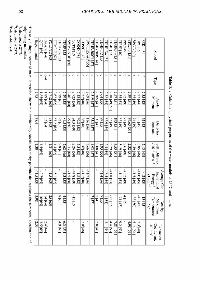
four main general model types are shown in Figure 3.8. Generally each model is de-veloped to fit well with one particular physical structure or parameter (for example, thedensity anomaly, radial distribution function or the critical parameters) and it comes asno surprise when a model developed to fit certain parameters it gives good compliancewith these same parameters [41]. In spite of the heavy computational investment in thecalculations, the final agreement with experimental data is often ‘by eye’ and not statis-tically tested or checked for parametric sensitivity. Also, tests for ‘quality’ often use theradial distribution fit with diffraction data in spite of the major fitted peaks being derivedfrom the tetrahedral nature of water that is built into every model and overpowers anydisagreement in the fine detail. In particular, the O—O radial distribution function seemsto be a poor discriminator between widely differently performing models [42]. Table 3.1shows the values predicted for some key water properties by some of the most popularwater force fields.

3.4.2 Implicit WaterThere are many circumstances in molecular modeling studies in which a simplified de-scription of solvent effects has advantages over the explicit modelling of each solventmolecule. Most of these are where the saving of computer time are needed over usingexplicit water. Most of the simulation techniques have models in which the solute de-grees of freedom are treated explicitly but the solvent degrees of freedom are not. Thisrequires that the energy surface used for the protein degrees of freedom be a potentialof mean force (PMF) in which the solvent degrees of freedom are implicitly averagedover [66]. Assuming that the full potential energy function consists of a term, Uvac forthe interactions within the protein, depending only on the protein degrees of freedom, r,and an additional term for the protein-solvent and solvent-solvent interactions, the PMFis ideally equation 3.4.1, whereDeltaGsol (r) is the free energy of transferring the proteinfrom vacuum to the solvent with its internal degrees of freedom fixed at r.

UPMF (r) = Uvac (r) + ∆Gsol (r) (3.4.1)

Some of the main models are:

COSMO Model [67] treats the solvent as a high dielectric continuum, interacting withcharges that are embedded in solute molecules of lower dielectric. In spite of theseverity of the approximation, this model often gives a good account of equilibriumsolvation energetics.

Poisson-Boltzmann Model [68] describes electrostatic interactions in a multiple-dielectricenvironment and are typically solved by finite-difference or boundary element nu-merical methods. These can be efficiently solved for small molecules but may be-come expensive for proteins or nucleic acids. Although progress continues to be

3.4. WATER MODELS 57

made in numerical solutions, there is a clear interest in exploring more efficient, ifapproximate, approaches to this problem.

Generalized Born Model [69, 70] computes the electrostatic work required to move acharged sphere from a vacuum environment into a continuous dielectric region. Theresult is proportional to the square of the charge and is inversely proportional to thesize of the ion. The basis of generalized Born theory is to extend these ideas to non-spherical molecules by casting the electrostatic contribution to solvation. The Bornmodel have not traditionally considered salt effects, but the model has be extendedto low-salt concentrations [71]. The key to making Generalized Born calculationsmore accurate (in the sense of agreement with Poisson-Boltzmann calculations) isimproved estimation of the effective Born radii [72].


Table3.1:

Calculated

physicalpropertiesofthe

waterm

odelsat25

◦Cand

1atm

.

Model

TypeD

ipoleM

oment

Dielectric

constantSelf

Diffusion

/10−

5cm2s −

1

Average

Con-

figurationalE

nergy/

kJmol −

1

Density

Maxim

umTem

perature/ ◦C

Expansion

Coefficient,

10−

4◦C−

1

SSD[43]

- 12.35

[43]72

[43]2.13

[43]-40.2

[43]-13

[43]-

SPC[39]

a2.27

[44]65

[45]3.85

[46]-41.0

[45]-45

[47]7.3

2[48]SPC

/E[49]

a2.35

[49]71

[49]2.49

[46]-41.5

[49]-38

[50]5.14

[51]SPC

/Fw4[51]

a2.39

[51]79.63

[51]2.32

[51]-

-4.98

[51]PPC

4[49]b

2.52[49]

77[49]

2.6[49]

-43.2[49]

4[52]

-T

IP3P[40]

a2.35

[53]82

[49]5.19

[46]-41.1

[53]-91

[47]9.2

[53]T

IP3P/Fw4[51]

a2.57

[51]193

[51]3.53

[51]-

-7.81

[51]T

IP4P[53]

c2.18

[49,53]53

[49]3.29

[46]-41.8

[53]-25

[53]4.4

[53]T

IP4P-Ew

[54]c

2.32[54]

62.9[54]

2.4[54]

-46.5[54]

1[54]

3.1[54]

TIP4P-FQ

[55]c

2.64[55]

79[55]

1.93[55]

-41.4[56]

7[55]

-T

IP4P/2005[41]

c2.305

[41]60

[41]2.08

[41]-

5[41]

2.8[41]

TIP4P/2005f[57]

c2.319

[57]55.3

[57]1.93

[57]-

7[57]

-SW

FLE

X-A

I 4[56]c

2.69[56]

116[56]

3.66[56]

-41.7[56]

--

CO

S/G3

[48]c

2.572[48]

882[48]

2.62[48]

-41.12[48]

-7.0

2[48]C

OS/D

[58]c

2.43[58]

69.8[58]

2.5[58]

-41.8[58]

--

GC

PM4[59]

c2.723

[59]84.3

[59]2.26

[59]-44.8

[59]-13

[59]-

SWM

4-ND

P4[60]

c2.461

[60]79

[60]2.33

[60]-41.5

[60]-

-T

IP5P[53]

d2.29

[53]81.5

[53]2.62

[46]-41.3

[53]4

[53]6.3

[53]T

IP5P-Ew

[61]d

2.29[61]

92[61]

2.8[61]

-8

[61]4.9

[61]T

TM

2-F[62]

c2.67

[62]67.2

[62]1.4

[62]-45.1

[62]-

-PO

L5/T

Z4[63]

d2.712

[63]98

[63]1.81

[63]-41.5

[63]25

[63]-

Six-site[64]

c+d1.89

3[64]33

3[64]-

-14

3[64]2.4

3[64]Q

CT

[65]a

1.852[65]

-1.5

2[65]-42.7

2[65]10

2[65]3.5

2[65]E

xperimental

-2.95

78.42.30

-41.5[53]

3.9842.53

1Has

onlya

single,center

ofm

ass,interaction

sitew

itha

tetrahedrallycoordinated

stickypotential

thatregulates

thetetrahedral

coordinationof

neighboringm

olecules2C

alculatedat27

◦C3C

alculatedat20

◦C4Polarizable

model

3.5. COARSE-GRAINING 59

3.5 Coarse-GrainingEven though computational power is rapidly increasing, with hardware performance dou-bling every two years [73] (technically the number of transistors doubling), coupled to thedevelopment of ever more efficient algorithms to deliver faster and more accurate calcu-lations; there is a pressing need to simulate chemical systems over timescales that go farbeyond those currently obtainable with atomistic systems.

The basic concept of coarse graining involves a reduction of the number of sites in asystem. This not only allows for smaller computational load, but also leads to a loss of finedetail in the system. There has to be a delicate balance between these two things, ideallyleading to a considerable speed up of the calculation while still preserving the necessarychemical and physical information. Decreasing the number of the interaction sites in amodel allows a significant speed up in the calculation. Computer time approximatelyscales as N2 (N is a number of interaction sites) for pairwise potentials. Additionally,some intermolecular movements are lost, allowing the system to explore phase spacefaster. A third speed up is due to the increase of time step for the calculation, as thevibration frequency of larger particles is slower.

In chemistry, a coarse grained system will typically still be represented at the molec-ular level, as prediction of local properties of the system is dependent on the presence ofmolecules. A common type of coarse grained model represents of a group of atoms witha single interaction centre, a so called “super atom”. These super atoms are then assignedinteraction parameters. The parameters are derived from a smaller scale, higher resolutionmodel of the system. Additionally, they may be fitted to the experimental values. Resultsof the calculation are dependant on them, so care should be taken when parametrizing thesystem.

Figure 3.9: Illustration of the coarse grain-ing procedure: sampling of a high resolutionmodel, analysis of the trajectory, mapping tolow resolution, iterative refining of the po-tential.

Currently there is only one readilyavailable coarse grained force field, MAR-TINI [74]. The force field is designed to beused in biomolecular simulations of lipids,proteins and carbohydrates [75–77]. Themodel uses a shifted Lennard-Jones 12-6potential with parameters fitted to free en-ergies of vaporisation, hydration and sepa-ration between water and organic solventsat room (300 K) temperature only. Thereare criticisms of water in this model due toits inability to remain in the liquid state inmembrane pores [78, 79]. Recently a moresophisticated, polarizable water model wasdeveloped by the same group [80]. Wateris proving to be one of the most difficultsystems to coarse grain, as finding poten-tials capable of exhibiting the correct be-haviour is difficult; though several effortshave been made recently [81–83].

The main constraint of coarse grainedpotentials is the limited transferability between different systems and thermodynamic con-ditions. Transferability is highly dependent on the system parametrised, and is generallybetter for finer grained models; for polymer systems transferability is not greatly affectedby a change in the length of the polymer chain [84].


To derive a suitable coarse grain potential, one would normally follow the general pro-cedure, shown in the Figure 3.9. A smaller scale, higher resolution atomistic (sometimesunited-atom) model is sampled using molecular dynamics or Monte Carlo simulations.When setting up the initial calculation and then mapping the system, it is important con-sider which properties are needed and at which time and length scales. The trajectoriesfrom high resolution calculation are then analysed and the starting potentials for the coarsegrain model are obtained. For most of the cases it is necessary to refine the latter to obtainconsistent results with the higher resolution method.

3.5.1 MappingIn the mapping procedure, one represents a group of atoms with a single interaction centre.This centre is called a super atom and commonly positioned at the centre of mass of thegroup of initial atoms. Super atoms, as in atomistic calculations, are interlinked withsprings and follow the same rules of Newtonian mechanics. The choice of atoms to groupinto a bead is typically done by geometrical examination of the molecule and leads to acoarse grained molecule still resembling the general shape of the initial molecule. Thiswill allow a better agreement of non bonded properties. Additionally, one should considerwhich interactions form the simplest, if possible single well or simple shape potentials,that will be beneficial in refining the system in further iterative steps [85]. The parts ofthe molecule that are geometrically mobile (eg. undergoing gauche–trans conformationalchanges) will typically lead to potentials with more then one well.

3.5.2 PotentialsWhen the mapping is chosen, the next step is to evaluate the optimum parameters to de-scribe the interactions between the coarse grained sites. Over the last few years a numberof approaches have been developed:

Force matching , where a multibody potential of mean force of a high resolution systemis matched by a low resolution one [86]. This approach looks at individual config-urations, rather than the average properties of the system as encompassed by radialdistribution functions [87, 88].

Inverse Monte Carlo , where the new parameters are fitted by the use of Monte Carlocalculations [89, 90]. The potentials are derived from distributions, e.g.% bondlength, angle, dihedral angle, and radial distribution functions.

Iterative Boltzmann Inversion , where the new parameters are fitted with the aid ofmolecular dynamics calculations [91]. The potentials are derived from distribu-tions, e.g. bond length, angle, dihedral angle, and radial distribution functions.

3.5.3 Iterative Boltzmann InversionIterative Boltzmann Inversion is a structure based method and is aimed at matching dis-tribution functions of a new coarse grained model to a higher resolution calculation or ex-periment. Bonded interactions (bond, angle and dihedral) incorporate neglected degreesof freedom and temperature effects. Non-bonded are calculated separately, creating phys-ically sensible interactions between molecules. Generally, bonded potentials are strongerthan non bonded ones. The fitting of the potentials should start with the strongest one

3.6. REFERENCES 61

(deepest potential well), as it will change the least during fitting of the rest, hence theorder:

Pbond → Pangle → Pdihedral → Pnonbonded

Figure 3.10: Illustrated procedure for deriv-ing effective potentials by the iterative Boltz-mann inversion (IBI) method.

Figure 3.10 illustrates the procedurefor deriving an effective potential V (x)from a known probability distribution,Pref (x). P (x) is a general term for thedistribution, that could be a radial distri-bution function, g(r); bond length, b(r);angle, a(θ); or dihedral angle, d(φ); distri-bution.

For the first step of the iteration, areasonable guess of an effective potentialshould be obtained. This can be derivedfrom a reference probability, Pref (x), of ahigh resolution simulation of a pure sys-tem, equation 3.5.1.

V0 (x) = −kBT lnPref (x) (3.5.1)

It should be mentioned that V0 is nota potential energy, but rather a free en-ergy, dependant on temperature and pres-sure. V0 is a reasonable guess for the firstcoarse grained potential. A coarse grainedsimulation is performed and new probabil-ity distributions Pi (x) evaluated. The newdistribution will differ from Pref (x) andso the new potential should include a cor-rection, in order to provide a better repre-sentation of the system equation 3.5.2 isused, where λ is a numerical scaling factor and should be λ ∈ (0, 1].

Vi+1 (x) = Vi (x)− λkBT lnPi (x)

Pref (x)(3.5.2)

The new calculation will again result in a probability distribution, Pi+1. The iterativeprocedure should be repeated until Pi+n is sufficiently close to Pref . It has been testedby numerous authors and shown that it can take up to 200 iterations to obtain a potentialcapable of representing aggregate distributions [92] and over 1000 iterations to recovercorrect potential functions [93].

3.6 References[1] Philip M. Morse. Diatomic Molecules According to the Wave Mechanics. II. Vibra-

tional Levels. Phys. Rev., 34:57–64, Jul 1929.

[2] Gustav Mie. Zur kinetischen Theorie der einatomigen KÃurper. Annalen der Physik,316(8):657–697, 1903.


[3] A. Warshel and S. Lifson. Consistent force field calculations. II. Crystal structures,sublimation energies, molecular and lattice vibrations, molecular conformations,and enthalpies of alkanes. The Journal of Chemical Physics, 53:582, 1970.

[4] David N.J. White. A computationally efficient alternative to the Buckingham poten-tial for molecular mechanics calculations. Journal of Computer-Aided MolecularDesign, 11:517–521, 1997. 10.1023/A:1007911511862.

[5] J. E. Jones. On the Determination of Molecular Fields. I. From the Variation of theViscosity of a Gas with Temperature. Proceedings of the Royal Society of London.Series A, 106(738):441–462, 1924.

[6] H. A. Lorentz. Ueber die Anwendung des Satzes vom Virial in der kinetischenTheorie der Gase. Annalen der Physik, 248(1):127–136, 1881.

[7] Robert J. Good and Christopher J. Hope. New Combining Rule for IntermolecularDistances in Intermolecular Potential Functions. The Journal of Chemical Physics,53(2):540–543, 1970.

[8] B. E. F. Fender and Jr. G. D. Halsey. Second Virial Coefficients of Argon, Kryp-ton, and Argon-Krypton Mixtures at Low Temperatures. The Journal of ChemicalPhysics, 36(7):1881–1888, 1962.

[9] William L. Jorgensen, David S. Maxwell, and Julian Tirado-Rives. Developmentand Testing of the OPLS All-Atom Force Field on Conformational Energeticsand Properties of Organic Liquids. Journal of the American Chemical Society,118(45):11225–11236, 1996.

[10] B. R. Brooks, C. L. Brooks, A. D. Mackerell, L. Nilsson, R. J. Petrella, B. Roux,Y. Won, G. Archontis, C. Bartels, S. Boresch, A. Caflisch, L. Caves, Q. Cui, A. R.Dinner, M. Feig, S. Fischer, J. Gao, M. Hodoscek, W. Im, K. Kuczera, T. Lazaridis,J. Ma, V. Ovchinnikov, E. Paci, R. W. Pastor, C. B. Post, J. Z. Pu, M. Schaefer,B. Tidor, R. M. Venable, H. L. Woodcock, X. Wu, W. Yang, D. M. York, andM. Karplus. CHARMM: The biomolecular simulation program. Journal of Compu-tational Chemistry, 30(10):1545–1614, 2009.

[11] Wendy D. Cornell, Piotr Cieplak, Christopher I. Bayly, Ian R. Gould, Kenneth M.Merz, David M. Ferguson, David C. Spellmeyer, Thomas Fox, James W. Caldwell,and Peter A. Kollman. A Second Generation Force Field for the Simulation ofProteins, Nucleic Acids, and Organic Molecules. Journal of the American ChemicalSociety, 117(19):5179–5197, 1995.

[12] A. K. Rappe, C. J. Casewit, K. S. Colwell, W. A. Goddard, and W. M. Skiff. UFF, afull periodic table force field for molecular mechanics and molecular dynamics sim-ulations. Journal of the American Chemical Society, 114(25):10024–10035, 1992.

[13] William L. Jorgensen and Julian. Tirado-Rives. The OPLS [optimized potentialsfor liquid simulations] potential functions for proteins, energy minimizations forcrystals of cyclic peptides and crambin. Journal of the American Chemical Society,110(6):1657–1666, 1988.

[14] Markus Christen, Philippe H. Hunenberger, Dirk Bakowies, Riccardo Baron, RolandBurgi, Daan P. Geerke, Tim N. Heinz, Mika A. Kastenholz, Vincent Krautler, ChrisOostenbrink, Christine Peter, Daniel Trzesniak, and Wilfred F. van Gunsteren. The

3.6. REFERENCES 63

GROMOS software for biomolecular simulation: GROMOS05. Journal of Compu-tational Chemistry, 26(16):1719–1751, 2005.

[15] M.G. Martin and J.I. Siepmann. Transferable potentials for phase equilibria. 1.United-atom description of n-alkanes. The Journal of Physical Chemistry B,102(14):2569–2577, 1998.

[16] Marcus G. and Martin. Comparison of the AMBER, CHARMM, COMPASS, GRO-MOS, OPLS, TraPPE and UFF force fields for prediction of vaporâASliquid coex-istence curves and liquid densities. Fluid Phase Equilibria, 248(1):50 – 55, 2006.

[17] Yong Duan, Chun Wu, Shibasish Chowdhury, Mathew C. Lee, Guoming Xiong, WeiZhang, Rong Yang, Piotr Cieplak, Ray Luo, Taisung Lee, James Caldwell, JunmeiWang, and Peter Kollman. A point-charge force field for molecular mechanics sim-ulations of proteins based on condensed-phase quantum mechanical calculations.Journal of Computational Chemistry, 24(16):1999–2012, 2003.

[18] Junmei Wang, Romain M. Wolf, James W. Caldwell, Peter A. Kollman, andDavid A. Case. Development and testing of a general amber force field. Journalof Computational Chemistry, 25(9):1157–1174, 2004.

[19] A. D. MacKerell, D. Bashford, Bellott, R. L. Dunbrack, J. D. Evanseck, M. J. Field,S. Fischer, J. Gao, H. Guo, S. Ha, D. Joseph-McCarthy, L. Kuchnir, K. Kuczera,F. T. K. Lau, C. Mattos, S. Michnick, T. Ngo, D. T. Nguyen, B. Prodhom, W. E.Reiher, B. Roux, M. Schlenkrich, J. C. Smith, R. Stote, J. Straub, M. Watanabe,J. Wiorkiewicz-Kuczera, D. Yin, and M. Karplus. All-Atom Empirical Potential forMolecular Modeling and Dynamics Studies of ProteinsâAa. The Journal of PhysicalChemistry B, 102(18):3586–3616, 1998.

[20] A.D. Mackerell Jr, M. Feig, and C.L. Brooks III. Extending the treatment of back-bone energetics in protein force fields: Limitations of gas-phase quantum mechanicsin reproducing protein conformational distributions in molecular dynamics simula-tions. Journal of computational chemistry, 25(11):1400–1415, 2004.

[21] A.D. MacKerell Jr, N. Banavali, and N. Foloppe. Development and current status ofthe CHARMM force field for nucleic acids. Biopolymers, 56(4):257–265, 2000.

[22] K. Vanommeslaeghe, E. Hatcher, C. Acharya, S. Kundu, S. Zhong, J. Shim, E. Dar-ian, O. Guvench, P. Lopes, I. Vorobyov, et al. CHARMM general force field: Aforce field for drug-like molecules compatible with the CHARMM all-atom addi-tive biological force fields. Journal of computational chemistry, 31(4):671–690,2010.

[23] III WH Reiher. Theoretical studies of hydrogen bonding. PhD thesis, Harvard Uni-versity, 1985.

[24] S.V. Sambasivarao and O. Acevedo. Development of OPLS-AA force field param-eters for 68 unique ionic liquids. Journal of Chemical Theory and Computation,5(4):1038–1050, 2009.

[25] Z. Xu, H.H. Luo, and D.P. Tieleman. Modifying the OPLS-AA force field to improvehydration free energies for several amino acid side chains using new atomic chargesand an off-plane charge model for aromatic residues. Journal of computationalchemistry, 28(3):689–697, 2007.


[26] Berk Hess, Carsten Kutzner, David van der Spoel, and Erik Lindahl. GROMACS4: Algorithms for Highly Efficient, Load-Balanced, and Scalable Molecular Simu-lation. Journal of Chemical Theory and Computation, 4(3):435–447, 2008.

[27] Wilfred F. van Gunsteren, S. R. Billeter, A. A. Eising, Philippe H. Hünenberger,P. Krüger, Alan E. Mark, W. R. P. Scott, and Ilario G. Tironi. Biomolecular Simula-tion: The GROMOS96 manual and user guide. 1996.

[28] Markus Christen, Philippe H. HÃijnenberger, Dirk Bakowies, Riccardo Baron,Roland BÃijrgi, Daan P. Geerke, Tim N. Heinz, Mika A. Kastenholz, Vincent Kraut-ler, Chris Oostenbrink, Christine Peter, Daniel Trzesniak, and Wilfred F. van Gun-steren. The GROMOS software for biomolecular simulation: GROMOS05. Journalof Computational Chemistry, 26(16):1719–1751, 2005.

[29] M.G. Martin and J.I. Siepmann. Novel configurational-bias Monte Carlo method forbranched molecules. Transferable potentials for phase equilibria. 2. United-atom de-scription of branched alkanes. The Journal of Physical Chemistry B, 103(21):4508–4517, 1999.

[30] C.D. Wick, M.G. Martin, and J.I. Siepmann. Transferable potentials for phase equi-libria. 4. United-atom description of linear and branched alkenes and alkylbenzenes.The Journal of Physical Chemistry B, 104(33):8008–8016, 2000.

[31] B. Chen, J.J. Potoff, and J.I. Siepmann. Monte Carlo calculations for alcohols andtheir mixtures with alkanes. Transferable potentials for phase equilibria. 5. United-atom description of primary, secondary, and tertiary alcohols. The Journal of Phys-ical Chemistry B, 105(15):3093–3104, 2001.

[32] J.M. Stubbs, J.J. Potoff, and J.I. Siepmann. Transferable potentials for phase equi-libria. 6. United-atom description for ethers, glycols, ketones, and aldehydes. TheJournal of Physical Chemistry B, 108(45):17596–17605, 2004.

[33] C.D. Wick, J.M. Stubbs, N. Rai, and J.I. Siepmann. Transferable potentials for phaseequilibria. 7. Primary, secondary, and tertiary amines, nitroalkanes and nitrobenzene,nitriles, amides, pyridine, and pyrimidine. The Journal of Physical Chemistry B,109(40):18974–18982, 2005.

[34] N. Lubna, G. Kamath, J.J. Potoff, N. Rai, and J.I. Siepmann. Transferable potentialsfor phase equilibria. 8. United-atom description for thiols, sulfides, disulfides, andthiophene. The Journal of Physical Chemistry B, 109(50):24100–24107, 2005.

[35] B. Chen and J.I. Siepmann. Transferable potentials for phase equilibria. 3. Explicit-hydrogen description of normal alkanes. The Journal of Physical Chemistry B,103(25):5370–5379, 1999.

[36] N. Rai and J.I. Siepmann. Transferable potentials for phase equilibria. 9. Explicithydrogen description of benzene and five-membered and six-membered heterocyclicaromatic compounds. The Journal of Physical Chemistry B, 111(36):10790–10799,2007.

[37] J. D. Bernal and R. H. Fowler. A Theory of Water and Ionic Solution, with ParticularReference to Hydrogen and Hydroxyl Ions. Journal of Chemical Physics, 1:515–548, 1933.

3.6. REFERENCES 65

[38] F. H. Stillinger and A. Rahman. Improved simulation of liquid water by moleculardynamics. Journal of Chemical Physics, 60:1545–1557, 1974.

[39] H. J. C. Berendsen, J. P. M. Postma, W. F. van Gunsteren, and J. Hermans. Inter-molecular Forces. Reidel, Dordrecht, 1981.

[40] W. L. Jorgensen, J. Chandrasekhar, J. D. Madura, R. W. Impey, and M. L. Klein.Comparison of simple potential functions for simulating liquid water. Journal ofChemical Physics, 79:926–935, 1983.

[41] J. L. F. Abascal and C. Vega. A general purpose model for the condensed phases ofwater: TIP4P/2005. Journal of Chemical Physics, 123:234505, 2005.

[42] P. E. Mason and J. W. Brady. “Tetrahedrality” and the relationship between collec-tive structure and radial distribution functions in liquid water. Journal of PhysicalChemistry B, 111:5669–5679, 2007.

[43] M-L. Tan, J. T. Fischer, A. Chandra, B. R. Brooks, and T.ÂaIchiye. A temperatureof maximum density in soft sticky dipole water. Chemical Physics Letters, 376:646–652, 2003.

[44] K. Kiyohara, K. E. Gubbins, and A. Z. Panagiotopoulos. Phase coexistence proper-ties of polarizable water models. Molecular Physics, 94:803–808, 1998.

[45] D. van der Spoel, P. J. van Maaren, and H. J. C. Berendsen. A systematic study ofwater models for molecular simulation: Derivation of water models optimized foruse with a reaction field. Journal of Chemical Physics, 108:10220–10230, 1998.

[46] M. W. Mahoney and W. L. Jorgensen. Diffusion constant of the TIP5P model ofliquid water. Journal of Chemical Physics, 114:363–366, 2001.

[47] C. Vega and J. L. F. Abascal. Relation between the melting temperature and thetemperature of maximum density for the most common models of water. Journal ofChemical Physics, 123:144504, 2005.

[48] H. Yu and W. F. van Gunsteren. Charge-on-spring polarizable water models re-visited: from water clusters to liquid water to ice. Journal of Chemical Physics,121:9549–9564, 2004.

[49] H. J. C. Berendsen, J. R. Grigera, and T. P. Straatsma. The missing term in effectivepair potentials. Journal of Physical Chemistry, 91:6269–6271, 1987.

[50] L. A. Baez and P. Clancy. Existence of a density maximum in extended simplepoint-charge water. Journal of Chemical Physics, 101:9837–9840, 1994.

[51] Y. Wu, H. L. Tepper, and G. A. Voth. Flexible simple point-charge water modelwith improved liquid state properties. Journal of Chemical Physics, 124Âa:024503,2006.

[52] I. M. Svishchev, P. G. Kusalik, J. Wang, and R. J. Boyd. Polarizable point-chargemodel for water. Results under normal and extreme conditions. Journal of ChemicalPhysics, 105:4742–4750, 1996.

[53] M. W. Mahoney and W. L. Jorgensen. A five-site model for liquid water and thereproduction of the density anomaly by rigid, nonpolarizable potential functions.Journal of Chemical Physics, 112:8910–8922, 2000.


[54] H. W. Horn, W. C. Swope, J. W. Pitera, J. D. Madura, T. J. Dick, G. L. Hura, andT. Head-Gordon. Development of an improved four-site water model for biomolec-ular simulations. Journal of Chemical Physics, 120:9665–9678, 2004.

[55] S. W. Rick. Simulation of ice and liquid water over a range of temperatures usingthe fluctuating charge model. Journal of Chemical Physics, 114:2276–2283, 2001.

[56] P. J. van Maaren and D. van der Spoel. Molecular dynamics of water with novelshell-model potentials. Journal of Physical Chemistry B, 105:2618–2626, 2001.

[57] M. A. González and J. L. F. Abascal. A flexible model for water based onTIP4P/2005. Journal of Chemical Physics, 135:224516, 2011.

[58] A.-P. E. Kunz and W. F. van Gunsteren. Development of a nonlinear classical pPolar-ization model for liquid water and aqueous solutions: COS/D. Journal of PhysicalChemistry A, 113:11570–11579, 2009.

[59] P. Paricaud, M. Predota, A. A. Chialvo, and P. T. Cummings. From dimer and con-densed phases at extreme conditions: Accurate predictions of the properties of waterby a Gaussian charge polarizable model. Journal of Chemical Physics, 122:244511,2005.

[60] G. Lamoureux, E. Harder, I. V. Vorobyov, B. Roux, and A. D. MacKerell Jr. Apolarizable model of water for molecular dynamics simulations of biomolecules.Chemical Physics Letters, 418:241–245, 2005.

[61] S. W. Rick. A reoptimization of the five-site water potential (TIP5P) for use withEwald sums. Journal of Chemcal Physics, 120:6085–6093, 2004.

[62] G. S. Fanourgakis and S. S. Xantheas. The flexible, polarizable, Thole-type inter-action potential for water (TTM2-F) revisited. Journal of Physical Chemistry A,110:4100–4106, 2006.

[63] H. A. Stern, F. Rittner, B. J. Berne, and R. A. Friesner. Combined fluctuating chargeand polarizable dipole models: Application to a five-site water potential function.Journal of Chemical Physics, 115:2237–2251, 2001.

[64] H. Nada and J. P. J. M. van der Eerden. An intermolecular potential model for thesimulation of ice and water near the melting point: A six-site model of H2O. Journalof Chemical Physics, 118:7401–7413, 2003.

[65] S. Y. Liem, P. L. A. Popelier, and M. Leslie. Simulation of liquid water using a high-rank quantum topological electrostatic potential. International Journal of QuantumChemistry, 99:685–694, 2004.

[66] B Roux and T. Simonson. Biophysical Chemistry, 78:1–20, 1999.

[67] A. Klamt and G. Schüürmann. J Chem. Soc. Perkin Trans, 2:799–805, 1993.

[68] C. J. Cramer and D. G. Truhlar. Chemical Reviews, 99:2161–2200, 1999.

[69] M. Born. Z. Phys., 1:45–48, 1920.

[70] D. Bashford and D. Case. Annu. Rev. Phys. Chem., 51:129–152, 2000.

3.6. REFERENCES 67

[71] J. Srinivasan, M. W. Trevathan, P. Beroza, and D. A. Case. Theor. Chem. Ace.,101:126–434, 1999.

[72] M. S. Lee, F. R. Salsbury Jr, and C. L. Brooks III. Journal of Physical Chemistry,116,:10606–10614, 2002.

[73] G. E. Moore. Cramming more components onto integrated circuits. Electronics,38:114–117, 1965.

[74] S.J. Marrink, A.H. de Vries, and A.E. Mark. Coarse grained model for semiquan-titative lipid simulations. The Journal of Physical Chemistry B, 108(2):750–760,2004.

[75] S.J. Marrink, H.J. Risselada, S. Yefimov, D.P. Tieleman, and A.H. De Vries. TheMARTINI force field: coarse grained model for biomolecular simulations. TheJournal of Physical Chemistry B, 111(27):7812–7824, 2007.

[76] L. Monticelli, S.K. Kandasamy, X. Periole, R.G. Larson, D.P. Tieleman, and S.J.Marrink. The MARTINI coarse-grained force field: extension to proteins. Journalof Chemical Theory and Computation, 4(5):819–834, 2008.

[77] C.A. López, A.J. Rzepiela, A.H. de Vries, L. Dijkhuizen, P.H. Hünenberger, and S.J.Marrink. Martini coarse-grained force field: extension to carbohydrates. Journal ofChemical Theory and Computation, 5(12):3195–3210, 2009.

[78] M. Winger, D. Trzesniak, R. Baron, and W.F. Van Gunsteren. On using a too largeintegration time step in molecular dynamics simulations of coarse-grained molecularmodels. Phys. Chem. Chem. Phys., pages 1934–1941, 2009.

[79] Wilfred F. van Gunsteren and Moritz Winger. Reply to the ’Comment on "On using atoo large integration time step in molecular dynamics simulations of coarse-grainedmolecular models"’ by S. J. Marrink, X. Periole, D. Peter Tieleman and Alex H. deVries, Phys. Chem. Chem. Phys., 2010, 12, DOI: 10.1039/b915293h. Phys. Chem.Chem. Phys., 12:2257–2258, 2010.

[80] S.O. Yesylevskyy, L.V. Schäfer, D. Sengupta, and S.J. Marrink. Polarizable watermodel for the coarse-grained MARTINI force field. PLoS computational biology,6(6):e1000810, 2010.

[81] Leonardo Darre, Matias R. Machado, Pablo D. Dans, Fernando E. Herrera, andSergio Pantano. Another Coarse Grain Model for Aqueous Solvation: WAT FOUR?Journal of Chemical Theory and Computation, 6(12):3793–3807, 2010.

[82] AJ and Rader. Coarse-grained models: getting more with less. Current Opinionin Pharmacology, 10(6):753 – 759, 2010. <ce:title>Endocrine and metabolic dis-eases/New technologies - the importance of protein dynamics</ce:title>.

[83] S. Riniker and W.F. van Gunsteren. A simple, efficient polarizable coarse-grainedwater model for molecular dynamics simulations. The Journal of chemical physics,134:084110, 2011.

[84] P. Carbone, H.A.K. Varzaneh, X. Chen, and F. Müller-Plathe. Transferability ofcoarse-grained force fields: The polymer case. The Journal of chemical physics,128:064904, 2008.


[85] V.A. Harmandaris, D. Reith, N.F.A. van der Vegt, and K. Kremer. Comparisonbetween coarse-graining models for polymer systems: Two mapping schemes forpolystyrene. Macromolecular chemistry and physics, 208(19/20):2109, 2007.

[86] F. Ercolessi and J.B. Adams. Interatomic potentials from first-principles calcula-tions: the force-matching method. EPL (Europhysics Letters), 26:583, 1994.

[87] S. Izvekov and G.A. Voth. A multiscale coarse-graining method for biomolecularsystems. The Journal of Physical Chemistry B, 109(7):2469–2473, 2005.

[88] S. Izvekov and G.A. Voth. Multiscale coarse graining of liquid-state systems. TheJournal of chemical physics, 123:134105, 2005.

[89] A.P. Lyubartsev and A. Laaksonen. Calculation of effective interaction potentialsfrom radial distribution functions: A reverse Monte Carlo approach. Physical Re-view E, 52(4):3730, 1995.

[90] C.D. Berweger, W.F. van Gunsteren, and F. Müller-Plathe. Force field parametriza-tion by weak coupling. Re-engineering SPC water. Chemical physics letters, 232(5-6):429–436, 1995.

[91] D. Reith, M. Pütz, and F. Müller-Plathe. Deriving effective mesoscale potentialsfrom atomistic simulations. Journal of computational chemistry, 24(13):1624–1636,2003.

[92] A.J. Rzepiela, M. Louhivuori, C. Peter, and S.J. Marrink. Hybrid simulations: com-bining atomistic and coarse-grained force fields using virtual sites. Phys. Chem.Chem. Phys., 2011.

[93] S. Jain, S. Garde, and S.K. Kumar. Do inverse Monte Carlo algorithms yield thermo-dynamically consistent interaction potentials? Industrial & engineering chemistryresearch, 45(16):5614–5618, 2006.

Molecular Interactions - University of Manchester

Documents

Transcript of Molecular Interactions - University of Manchester