Series in BioEngineering

For further volumes:http://www.springer.com/series/10358

M. M. Kaila • Rakhi Kaila

Molecular Imagingof the Brain

Using Multi-Quantum Coherence andDiagnostics of Brain Disorders

123

M. M. KailaSchool of PhysicsUniversity of New South WalesSydney, NSWAustralia

Rakhi KailaSchool of MedicineUniversity of New South WalesSydney, NSWAustralia

ISBN 978-3-642-30301-2 ISBN 978-3-642-30302-9 (eBook)DOI 10.1007/978-3-642-30302-9Springer Heidelberg New York Dordrecht London

Library of Congress Control Number: 2012940233

� Springer-Verlag Berlin Heidelberg 2013This work is subject to copyright. All rights are reserved by the Publisher, whether the whole or part ofthe material is concerned, specifically the rights of translation, reprinting, reuse of illustrations,recitation, broadcasting, reproduction on microfilms or in any other physical way, and transmission orinformation storage and retrieval, electronic adaptation, computer software, or by similar or dissimilarmethodology now known or hereafter developed. Exempted from this legal reservation are briefexcerpts in connection with reviews or scholarly analysis or material supplied specifically for thepurpose of being entered and executed on a computer system, for exclusive use by the purchaser of thework. Duplication of this publication or parts thereof is permitted only under the provisions ofthe Copyright Law of the Publisher’s location, in its current version, and permission for use must alwaysbe obtained from Springer. Permissions for use may be obtained through RightsLink at the CopyrightClearance Center. Violations are liable to prosecution under the respective Copyright Law.The use of general descriptive names, registered names, trademarks, service marks, etc., in thispublication does not imply, even in the absence of a specific statement, that such names are exemptfrom the relevant protective laws and regulations and therefore free for general use.While the advice and information in this book are believed to be true and accurate at the date ofpublication, neither the authors nor the editors nor the publisher can accept any legal responsibility forany errors or omissions that may be made. The publisher makes no warranty, express or implied, withrespect to the material contained herein.

Printed on acid-free paper

Springer is part of Springer Science+Business Media (www.springer.com)

Foreword for the First Part of the Book:‘Quantum What Quantum Tell MeMore About It…….’

The routine MRI literature in the scientific world does not much emphasize MRI asa quantum coherence phenomena. The educational aspect of MRI does not depictwell the multi-quantum part of the nuclear magnetic resonance (NMR). Thenuclear multi-quantum aspect forms an integral part of the MQMRI (multi-quantum magnetic resonance imaging). The proper role of the word ‘Nuclear’ hasbeen avoided in the RF radiation imaging literature. The imaging is basicallyreferred to as the MRI instead of clearly mentioning the NMRI (nuclear magneticresonance imaging). This is done so as not to scare the patients. It was felt in thepast that patients may think that they are being exposed to dangerous nuclearradiations. MRI is as much an atomic as much a nuclear resonance phenomenon.The magnetic moment of protons in nuclei provide a rich source of informationabout the microscopic events happening in the brain, through spectroscopy as wellas imaging. The multi-quantum aspect of spectroscopy in an ensemble of mole-cules like our brain is well advanced and the imaging aspect is fast progressing.The MRI technology developed tries to emulate the functional system operative inthe brain. Nature has evolved the internal functional system operative in our bodyover millions of years. In MRI the investigation of the life functioning system isdone in a gentle way using radio frequency (RF) radiation. MRI does not involvebreaking the nuclei by using neutrons to produce fission of the nuclei which wouldthen lead to the production of dangerous nuclear radiations destructive to our body.This misconception had arisen due to the lack of populous education about thebasics of the science of MRI in particular, and also science as a whole. In fact, on awider scale the basic infrastructure of education about science for the new gen-eration of students is on the fast decline. Expansion in financial and bureaucraticfields like, accountancy, management, IT (information technology), etc., is fast onthe rise.

One must not forget that science leads to creation of the necessary literacyabout life itself on the one hand and develops practical inventions like the MRI

v

which is worth billion dollars of industry today on the other. The bureaucracy isdestructive to the creation of knowledge-based economy. Propagating scientificknowledge is the only way to survive today. Society is heading toward ignorantmisconceptions and neglect. What useful benefits of science the human civilizationshould adopt and leave others should be decided based on the proper educationabout the existing scientific balance that nature has created on earth. There is noother planet like earth in our universe. Better protect the one we have than trying toinvent another which you cannot make use of. MRI can detect soft organic andinorganic matter in addition to the rigid, e.g., the calcite structure like bones in ourbody. It can thus be a very useful method of detection involving security proce-dures in the aviation industry. We are a scientific civilization. Using science toproduce wealth is a constructive way of employing young minds. Just shoutingabout ‘climate change’ as a ‘political word’ of power is not going to produceanything. But starting education at the school level about the ‘science of climate’and science as a whole will produce an appropriate scientific manpower for thefuture to take right decisions.

MRI is only one among many visible commercial products from scienceworking in our day-to-day life. The scientific society we have developed ourselvesinto over the centuries cannot survive without science. There is no point indestroying the very foundation of humanity developed based on science. Natureitself has preferred science in its own evolution. Over time the present civilizationhas studied the secrets of nature, learnt them, and used them toward its ownbenefit. A freely available scientific-educational material produced by research anddevelopment work over the world would go a long way toward the education ofhumanity. The authors feel the work prepared here is a step in the right directionfor the future generations. Pretending that we do not need science is a shear act ofignorance. Survival of the human race today is only on education about science.One should realize that plant and animal life is the science of atoms and molecules.Deep inside it is the quantum science that nature builds on. It is what the MQMRIis based on. This is very much a quantum (in fact multi-quantum) phenomena. It isbetter to understand the quantum science of our body than to ignore it. Theconventional MRI uses quantum science as a wholesome, i.e., in a broaderquantum perspective. Assuming molecules in our brain as an ensemble of inde-pendent spins is the crudest model of the brain and that is what the conventionalMRI is about. It is natural for any technology to evolve starting from the simplestand the very fundamental basics. That is how the development of the MRI tech-nology has evolved. The mind can only start from the simplest, and then work outthe intricacies step-by-step. Nature itself has followed that in the evolution of life.The intricate discrete nature of atoms and molecules does not form the basis ofimaging in the conventional MRI of today.

The technology of MRI employs the use of noninvasive RF radiation. This is inorder to excite the nuclear and atomic magnets which are an integral part of thebiological structure of our brain. RF radiation is chosen because we are interestedin exciting atoms and molecules to their higher energy level. On returning back totheir normal or say zero energy state the RF radiation is transmitted back. The

vi Foreword for the First Part of the Book

receiver which is tuned to this out-coming radiation registers the events happeningin a local selected area under investigation. A point-by-point repetition over thewhole brain and coordinating the events over the global brain produces the picturewe are so familiar with. It is important to recognize here that the magnitude of theexcitation energy involved here is of the order of a few meV. One should comparethis with Mev (million electron volt) used in X-ray imaging. We live our day-to-day life on earth under the influence of the solar radiations with full electro-magnetic radiation spectrum and under the effects of the magnetic field of earth.Our life on earth exists in earth’s magnetic field of around 1 micro Tesla. This isvery small to think about having any dangerous effects on the human brain. Butinside our brain things on a similar scale are happening. There is no research tosuggest yet that this (Earth’s) small magnetic field in any way controls the routinefunctions happening in our brain. But it is curious enough to find out what does.MRI just tries to emulate it through imaging.

It is important to recognize that a nucleus as a part of an atom or of a mac-romolecule produces a field of about 1 Tesla around it. But this is over a region ofnm (nanometer) to micrometer scale. It decays fast over many molecular distances.But as the volume under consideration locally, becomes larger, the larger is thenumber of spins (remember a mole of a substance has 1023 spins) participating, ina particular activity. The result is that the effect of the decay of the field is not asfast as one would think. The distant spins as far as 1 micron to 1 mm distance caninfluence the local spins through a small distant dipole (spin)–dipole (spin) fieldindirectly created within by the applied external static magnetic field. In theMQMRI literature this new field is referred to as the distant dipole field (DDF).The distant spins produce a demagnetizing field at a point locally and generate theintermolecular multi-quantum phenomena. This is the basis of imaging in thenewly emerging MQMRI. Whether the earth’s magnetic field is already doing thisin the brain is what we are trying to find out? Would not it be nice to know?

The natural dipole–dipole interactions (DDI) in the brain can be studied usingthe proton magnetic resonance spectroscopy imaging (PMRSI). It is one of themany techniques available. The PMRSI technique utilizes mainly the nucleus, i.e.,the proton spin. The nucleus is part of the overall electron-atom-nucleus quantumstructure present in the brain. In the conventional concept of imaging, e.g., thechemical shift imaging (CSI), the atomic spins polarized along the direction of theapplied static magnetic field are being used as independent entities with no multi-quantum interaction between them to get the desired result. This is basically themacroscopic effect in the small regions (referred to as a voxel) of the order of mm3

and above. But in order to see the intricate events happening in the brain in spaceand time over smaller distances, i.e., the atomic distances, one needs to understandthe quantum interactions between atoms and molecules. The affective macromo-lecular distances, i.e., micron (10-6m) to mm is the region of the ‘multi-quantummagnetic resonance imaging (MQMRI) ’.

What MQMRI means is that one takes into account the explicit quantumreactions between atoms and molecules as the source of the imaging, and thecollected data is then more than just the broader imaging. This means getting close

Foreword for the First Part of the Book vii

to exactly what nature has created in our brain. That is what allows our bodyfunctions to continue on a moment-to-moment and day-to-day basis. We need tounderstand this nature’s, atomic level incredible quantum phenomena happeningin our brain to work out the right diagnostics and the treatment of diseases whichour brain suffers in our lifetime. In order to master the intricate quantum science oflife one needs to start from a standard textbook on quantum mechanics (QM).Also, the reader should refer to the recent research papers describing the science oflife as the quantum science (QS). For the reader, however, is presented below asimplified conceptual picture. It explains the basics of the multiple quantumcoherence (MQC). MQC exists between the molecules in our brain. It is a kind ofinteraction which allows various fundamental processes like metabolism, neuro-transmission, etc., to continue in our brain.

A: Single Quantum Coherence (SQC): (Conventional MRI)

The expression through illustration here is as if the whole brain has all the spins(tiny dipole magnets) pointing along the Z-direction, the direction along which thestatic magnetic field is applied. The spins are assumed to be identical in naturethough they are not. This is a crudest possible model. But one should rememberthat in the first stage we image the identity of the spins through their being presentin different environments. It is in space and time. The output signal is producedusing RF radiation pulses. A 90� pulse is applied along the X-direction. It leads toa rotation of a fraction of the spins pointing toward the Y-direction. Because of theoscillatory (pulse) nature of the RF radiation applied the output signal is also analternating current (A.C.) one. The signal is picked up as an output along the Y-direction by a copper coil or some other form of sensor. There is evolution of thespins after applying the RF radiation pulse in the X–Y plane. As time progressesevolution of spins leads to their dissociation as a group in the X–Y plane.

Y

RF radiation in

Modulated RFradiation comes outwith signatures of thelocal environment

Z

X

They are refocused by applying an inverting (180�) pulse inverting the spinstoward the –Y direction in the X–Y plane. It allows longer times to measure andanalyze them. This basically leads to mapping a specific (choosing a particularslice thickness in the Z-direction) X–Y plane. The relaxation time of the spins in

viii Foreword for the First Part of the Book

the X–Y plane is called the characteristic time, T2 (transverse relaxation time) ofdecay. In a similar fashion the spins are reversed by applying 180� pulse reversingspins toward the -Z direction and the spins are allowed to relax back toward the+Z direction. This characteristic time of relaxation is called the T1, the longitudinalrelaxation time. Both T1 and T2 weighted data in space is used in producing thefinal image. Repetition voxel-by-voxel over the whole brain produces the globalbrain image. These are the basics of the conventional MRI technique. A techniqueusing this principle in MRI is broadly referred to as the EPI (eco planar imaging)in MRI. Other concepts, e.g., correlating diffusion-based anisotropy of the spins,called tensor imaging, e.g., in a tumor situation are also prevalent in conventionalMRI. Refer to Section 6, for details about T1, T2, and the k-space imaging conceptused in MRI.

B: Double Quantum Coherence (DQC): (The MQMRI)

Y

X

ZInput RF Radiation hasresonance frequency, specificto the two spins, pointing inthe same direction, in a boundstate. It is called as the doublequantum coherence

Output RF radiation, ismodulated, by thesimultaneous interaction,of the bound groups, of the twobound spins, pointing in thesame direction.

In this case the expression through illustration about two spins pointing in the samedirection is considered as a bound group in action. Generally, nearby spinspointing in the same direction repel each other like two bar magnets with north–south poles pointing in the same direction. But there will be some spins furtheraway pointing in the same direction where the magnetic influence of the spins willbe attractive to each other. This in other words means quantum coherence (actingtogether for a specific activity say metabolism) in the quantum science language.This correlation or interaction of two parallel spins in a ‘group of two’ is called thedouble quantum coherence. This picture holds on a scale in the brain over dis-tances of microns to mms. One needs to see the in-depth picture of this two-spinbound state resonance. In a selected region we have to go to distances of the orderof a micron (10–6 m) and choose a resonance frequency corresponding to thisgroup-of-two-bound spins pointing in the same direction for the regional analysis.

Foreword for the First Part of the Book ix

C: Zero Quantum Coherence (ZQC): (The MQMRI)

Z

XY

Input RF radiation istuned in resonance to thebound-state of, the groupof two spins, pointing inthe opposite direction

Output RF radiation, is modulated bythe simultaneous quantum interactionsof, the groups of the two-spins, in thezero-quantum state. The zero-quantumstate, is due to, the two oppositelydirected spins, bound together.

This interaction group consists of two spins bound together with the spins pointingin the opposite direction to each other. The two nearby spins in an ensembleinfluence each other. One spin tends to reverse the direction of the other spin. Thisbound state is the lowest energy state for the two spins near (and far) to each other.The applied static magnetic field along the Z-direction tries to keep all the spinsaligned along the Z-direction. The spins pointing in the Z-direction is the equi-librium energy state of the spins. This oppositely directed binding of the spins nearand far is called the ZQC. This will have a unique resonance frequency. It can beexcited by externally applying a suitable RF magnetic field like in the case of DQCto the brain. The quantum interactions allow the quantum chemistry of nuclei to beobserved in space and time. Detection of the quantum interactions is very helpfulto predict in early stages the onset of a tumor or a disorder in our brain. ZQC ismagnetically neutral. It is insensitive to magnetic field inhomogeneities. It isconsidered to be a powerful quantum probing tool in the MRI.

D: Triple Quantum Coherence (TQC)

Z

X

Y

Input RF radiation is tuned tothe resonance frequency of, thegroup of three bound spins,pointing in the same direction, asa single quantum state

Output RF radiation is modulated, bythe group of three, simultaneouslyinteracting spins, quantum state

One can involve more than two spins, e.g., three or even four spins in a boundgroup. The triple-bound state will have a quantum energy structure of its own.

x Foreword for the First Part of the Book

Thus a unique resonance frequency of its own. One can excite the group of threebound-nuclei and study their interactions on a microscopic scale and predict whichway the local quantum chemistry is heading and make an early detection of acancer in the brain. One should remember that our brain is a heteronuclear(multiple species of nuclei) structure. Various nuclei present in a macromoleculeas part of a tissue, fluids, etc., are performing their routine duties of metabolism,neurotransmission, etc. The influence of interaction extended can be visualizedthrough analyzing the resonance of the TQC (triple quantum coherence) as a groupin a subvoxel space in the brain. As a bound group of spins becomes larger one isapproaching towards what the conventional imaging does. One may however beinterested in the detailed chemistry of the participation of a regional group ofnuclei. The chemical identity of nuclei due to their unique electronic structureprovides a probe to understand in-depth the science of the brain. This opportunityis provided by the triple-quantum coherence imaging. The word coherence meansin the literary sense acting together. In scientific knowledge it means exciting orstimulating simultaneously a group of atoms or nuclei which may be part of amacromolecule. We then find out what activity they are enhancing i.e. having aconstructive interference within a specific period of time and the others they aresuppressing (i.e. making a destructive interference). The unique resonance fre-quency of a macromolecule gets smeared out due to its constituent nuclei; thenuclei being of different identities. This group may be interacting with a neigh-boring group. The group–group interaction is through their common group-reso-nance (a wider band of frequencies). This gives rise to multiple quantumcoherences. It now is a broader frequency RF band. The RF radiation can bechosen to include as many widely dispersed nuclei one is interested in.

The quantum mechanical imaging (QMI) approach in MRI is a fast advancingarea and will one day be able to predict moment-to-moment events happening inthe brain. It is common knowledge that the MRI has its origin in using the quantumbehavior of the magnetic spins present in atoms and molecules. But the quantumnature of the MRI is evident explicitly only when one is dealing with ZQC, DQC,etc. The scientific literature in MRI loosely refers to molecular and atomic magnetsas spins. They are atomic size dipole-magnets which are globally present in thebrain and due to their random distribution overall neutralize themselves. Atomsand molecules, the constituent parts of the tissues, fluids including the blood cells,etc., are integral parts of the biological and medical activities happening in ourbrain, in equilibrium. The atomic spins are the natural result of the circular motionof the electrons around the nucleus in an atom. An electron by itself (due tointrinsic rotation about its own axis) makes an additional contribution of spin tothat due to the electron’s orbital motion around the nucleus. A nucleus also has itsown magnetism. It arises from the circulating electrical currents of neutron andprotons inside the nucleus.

The relative circular motion of the negative charge of the electron with respectto the positive charge of the nucleus produces locally a magnetic field of about 1Tesla. The internal magnetic field is strong enough to create a local magnetism inthe soft matter in the brain. The local magnetization created is called the

Foreword for the First Part of the Book xi

diamagnetism. The result is a local polarization. There is of the neighborly atomicand molecular spins some sort of local equilibrium due to this internal magneticfield. It controls the local events, e.g., metabolism, neurotransmission, etc. Naturehas cleverly manipulated this order on its own. How clever? One may say that weare still today on the path of slow evolution of life. It is true to say that. Nature haspassed on from generation to generation the secrets of survival of the human genecode and keeps on mutating it for survival in worse and worse scenario of diseases.It is for us to find out now ‘how and why’. The internal magnetic field of 1 Tesla ofa nucleus naturally present in our brain produces a local magnetic order of atomsand molecules in the brain on the micrometer scale. The MRI by its externallyapplied static magnetic field of around 3 Tesla and sometimes even higher(allowed within safe limits) extends the spatial order over larger spaces.

The MRI technology provides us with an easy tool to mimic nature’s operationof the brain system. This can be skillfully observed by the modern day MRItechnology. It is certainly a powerful tool to find out how our brain works. Thenatural internal static magnetic field creates a stable equilibrium of the spins overregions of the order of nanometers to micrometers to mms. The external magneticfield in the conventional MRI on the other hand produces rough regions of mag-netic equilibrium from mms to cms. These are the regions of externally imposeddiamagnetic equilibrium. This created diamagnetism in MRI, in the brain, is anatural consequence of the reaction of the atoms and molecules, to the appliedstatic magnetic and the dynamic RF fields. The reaction to the applied field is toshield or say to save the brain from any damage. How clever of nature. Thediamagnetism due to the internal nuclear magnetic field is basically neutralizedlocally as well as globally all over the brain. The application of the externalmagnetic field as is done in MRI mimics this invisible order over large volumes oforder, say mm3–cm3 termed as voxels. After the application of the static magneticfield an RF electromagnetic field is subsequently applied to the brain to excite themagnetic spins to their higher order quantum states. The quantum correlations ofthe neighboring atoms and molecules provide the basis of the advanced techniqueof MQMRI (multi-quantum magnetic resonance imaging). This becomes a sourceof better resolution in imaging as compared to the currently prevalent techniquesof chemical shift imaging (CSI), diffusion weighted imaging (DWI), etc. Theintensity variation of the echoes received acts as the sources of the signatures ofthe activities in the brain in conventional imaging. In multi-QMRI it is the finephysical and chemical quantum reactions in space and time that is the source ofimaging. In this way one is approaching the intricate situation present in the brain.A healthy brain works in a mysterious way. It can think, analyze, and control bodyfunctions in a judicious manner. But when diseased the functions of the brain areimpaired and it cannot perform in its full analytical capacity. The idea behindwriting this work is to implicate the basic principles of physics, chemistry, andmathematics (PCM) involved in the science of the human brain. MRI is a humbletool trying to solve the mysteries of nature. More often than not professionals andtechnical workers use MRI for analyzing human brain disorders.

xii Foreword for the First Part of the Book

MRI is a standard tool used in the diagnostics of tumors. Some workers in thefield do not really have a strong enough background of the PCM principles used inproducing an image. Hence, they are not able to make the best of the imageproduced. In this work effort is made to explain the concepts involved, throughpictures, diagrams, etc. The mathematics involved is kept to a minimum. Somesimple equations are included only as symbolic representations of the physicalquantities involved. Although MRI is based on the physics of the quantum natureof soft matter a detailed relationship to quantum science is avoided to keep thingssimple. Quantum information science (QIS) is emerging as a discipline wheredetailed quantum mechanical mathematics is used to study quantum systems. Thisis not the aim here. Here, the goal is to lay down simple concepts of quantumphysics and analyze their use in imaging the moment-to-moment activities in thebrain, etc. So far the imaging has been based on manipulating the maximummagnitude possible of the signals received from the echoes produced by the RFradiation in the brain space.

A small region is chosen at a time for examination called as a voxel. In thepresent day EPI (echo planar imaging), the voxel is macroscopic in size of aroundmm3–cm3. Recently, there is a growing trend in going toward a microscopic levelimaging. This means moving to narrower spacing of less than 1 mm3 to even lessthan a micron volume (10-6 m3). This brings us into a more rigorous territory ofquantum science in operation. The theoretical quantum details are avoided in thiswork. Instead pictures and diagrams are used for the expression. The quantum-detailed imaging provides a much better resolution than the conventional, broadrelaxation-time-based imaging. The MRI uses as a typical example a simple echo-planar imaging (EPI) method. It is a fast technique but lacks good resolution.Further developments in MRI depend on the continuous education of the profes-sionals who develop it and others who want to use it. This work has a simplifiedapproach to attract medical professionals to make better use of the science ofimaging in the diagnostic decision-making process. This work is also aimed atachieving a much wider circulation of the understanding of the basics of MRI andits application in turn through the enchanting knowledge of the science of thehuman brain.

Foreword for the First Part of the Book xiii

Preface for First Part of the Book

Humans on earth out of curiosity have developed powerful telescopes to look intothe structure of the universe around us. We are striving to look for signs of lifewhether in the galaxy in which we live or in other galaxies. Are we so special? Isthere need to be looking for our image billions and billions of kilometers away? Asa matter of curiosity and knowledge there is such a need. The dynamics of themotions of the stars, planets, etc., is explained by Newton’s gravitational laws andis a well-established science in theory and experiment. There is another aspect ofscience. We have several elements in the earth’s crust, e.g., iron, copper, calcium,sodium, potassium, silicon, etc. Some of these elements, e.g., sodium, potassium,chlorine, in the form of some compounds, etc., form an essential part of thesurvival of life, plant, or animal. We should look deep inside the atomic structureof the elements and of the molecules they form, e.g., the water molecule H2O, theessential ingredient for our survival. The dynamics of the electrons, protons, nucleiin our body is as intriguing as puzzling. For example, the electrons stay in stableorbits around the nuclei. It is no different from, say, the planet earth going aroundour Sun. One needs to go to nanometer distances (10-9) deep from the surface of amacromolecule to work out the amazing science inside the atoms and molecules.This branch of science which deals with the deep down discrete structure ofmatter, i.e., atoms and molecules, is called quantum science.

Quantum science also has its laws in nature worked out though not in as clear away as the gravitational ones. In a practical use, e.g., in our brain one can seequantum laws of dynamics as clearly brought out through MRI. They are related tosimple concepts in physics. The quantum magnetic resonance used in Magneticresonance imaging (MRI) is a typical example. As a machine, MRI is seen veryprevalent in hospitals, medical centers, universities, etc., as a part of our healthsystem. We can hardly miss to look at it through a diagnostic picture to find whathas gone wrong in our body when we fall sick. Multi-quantum spectroscopy whichreveals the multi-quantum structure of atoms and molecules is century old. It isnow being applied to in vivo brain imaging over the past of couple of decades. Itacts as a complement to find out the concentration and specific functional role ofvarious chemicals present in our brain. Multi-quantum coherence imaging (MQCI)

xv

does both (spectroscopy and imaging) together in an integrated form. This bookwhich has purely educational aim behind it tries to put together quantum scienceand the imaging of the brain together. For some readers, e.g., for clinicians to learnquantum science in-depth can be a difficult task. This book has avoided the phe-nomenological development of the physics, chemistry, and mathematics (PCM)that form a detailed exposure of brain imaging. The approach taken here instead, isto let the reader learn through practical visualization of the concepts in action.

xvi Preface for First Part of the Book

Preface for the Second Part of the Book

Nature has evolved though essential elements like oxygen, hydrogen, nitrogen,iron, zinc, etc., via their inorganic and organic compounds, e.g., NaCl, H2O, KCL,FeO, etc. There are various organic matter macromolecules encompassing thebasic isotopes, e.g., 1H, 13C, 23 Na, 35Cl, 31P, 39K, 57Fe, etc., which have regulatedthe animal and plant life evolved over millions of years on the earth. Deep down inlife which evolves all the time are tiny building blocks, atoms, and molecules,which conglomerate to form bigger molecules, the macromolecules, the tissue, andultimately the body. Atoms, when looked into deeply, have a nucleus with apositive charge at the center surrounded by negatively charged electrons. Themagnitude of the positive charge at the center of the nucleus (basically due to theprotons) is equal to the negative charge of the surrounding electrons. This keepsthe atoms and the molecules electrically neutral as it should. One should rememberthat there are always some ionized free radicals present in our body. The electronsin atomic and molecular situations are not stationary but orbit around the nucleusand stay in a number of stationary orbits so as not to collapse into the nucleus. Theorbital motion of an electron around the nucleus generates an electric current. Thiselectric current when multiplied by the area of the orbit of the electron is called themagnetic dipole (in analogy with the earth’s giant, the north–south pole dipole-magnet) moment. The tiny atomic dipole magnets in our body coordinate withother atoms to form bigger molecular magnets. The molecules expand theirelectron correlations with their surrounding molecules to form cohesive charge andspin configured macromolecules. The macromolecules which form the essentialpart of the dynamics of life in the human body (and even in the plants and animals)retain the feature of the magnetic (over a large molecular space) dipole character.These macromolecules are tens and hundreds of nano (10–9) m in size and controlthe dynamics of the life of all living creatures.

One needs to remember that orbital motion of electrons (and of protons andneutrons inside the nucleus) generates a basic physical quantity in motiondynamics, the angular momentum locally in macromolecules in our body. Thislocal basic physical quantity, the macromolecular angular momentum, becomesthe source of all the activities coordinated in the brain. The dipole magnetic

xvii

moment is a naturally associated part of the angular momentum. Unfortunately,angular momentum in the molecular situation cannot be measured in the labora-tory. But fortunately, nature is kind to let us find the secrets of life through themolecular dipole magnetic moment associated with the annular momentum.Nature’s secret is that the magnetic dipole moment creates electrical signals whichwe measure and help to create the MRI we know. How lucky are we? We are at thecenter of a vast universe which is formed of atoms and molecules. The atoms andmolecules have evolved over millions of years in such a way as to create the mostintelligent form of life on earth. Intelligence does not progress without a healthyscientific environment and the interaction of the body and mind with the universewhich surrounds us. The magnetic resonance (MR) phenomena observed throughMRI in our body is like many other resonance phenomenae observed in nature.These can be seen all around us and are used in many technologies, e.g., Radio andTV broadcast, Lasers, etc. The development of MR into a practical MRI machinewe are so familiar with now has been the result of more than half a century ofresearch and development efforts. It is now not only a routine health care tech-nology in hospitals and medical centers but is also a valuable noninvasive tool ofresearch and education about the science of the human body. Sodium is animportant element and there are several others found in almost every organ of thehuman body involved in the functioning of organs on a moment and day-to-daybasis.

Sodium nuclear magnetic resonance imaging (SNMRI) is now being used in thearea of diagnostics of diseases of several organs of the body, e.g., the brain, liver,heart, kidney, etc. In the present day MRI we have the single-quantum (conven-tional) MRI technology approach. It is a routine versatile technological tool in thediagnostics of the human brain disorders. It is important to point out here that thesingle quantum basically means that we assign a single resultant spin covering allthe spins of the group of molecules in a voxel (a small volume) under measure-ment. The dispersion in the output signal observed in time and space is the result ofthe various dynamic activities in the brain. These are measured by various tech-niques, e.g., the blood oxygen level dependence MRI, called the fMRI (functionalMRI), SNMRI, etc.

The multi-quantum means the subvoxel molecular level structure dynamics. Itdoes not form part of the present (conventional) MRI technology. MRI enablesscientific research follow-up through monitoring the effects of a treatment therapy.During the practice of following this research scientists discover new and bettertreatments for a disorder. A useful secretive knowledge gathered through the MRIabout our brain creates literacy about our brain and how it works. In essence, in theconventional MRI, which we have at present one is looking for the spin (tinyatomic and molecular magnets) interactions over the wider average volume (mm3–cm3) as the medium in which they reside and move. This medium provides theenvironment of generation of the spin electrical signals. Through the brain mediumof tissues, fluids, etc., spins perform dynamic activities, e.g., metabolism, com-munication, etc. In the conventional MRI model we assume spins behave like anaveraged entity over a selected volume. Over the voxel-to-voxel situation they are

xviii Preface for the Second Part of the Book

magnetic entities with little multi-quantum interactions with other molecular spins.Their imaging identity is through their interaction with the environment in whichthey respond to the applied static magnetic field and the radio frequency (RF)radiation that is applied.

The physical and chemical multi-quantum interactions on a molecular levelbetween spins are of little consideration in the conventional MRI. The result ismore like mapping rather than a picture of the precise dynamical events happeningin the brain. This is the limit (called as single quantum) on which the conventionalMRI has been founded. In-depth MRI would allow one to understand the basicscience of the human brain. Sodium and potassium are very basic elementsinvolved in life controlling the familiar sodium–potassium pump in our body.They perform essential energy transport and metabolic functions for the naturallife-running mechanisms in the body. Typically in the brain, e.g., in the ischemicsituation, it is known that the healthy natural sodium concentration inside the cellmembrane is disturbed. There is extra uptake of sodium ions in the cell inside atissue than the healthy normal balance requires. The life giving sodium–potassiumequilibrium pump then does not perform in a normal healthy manner, anymore.The brain becomes disordered and the person ends up with a stroke. Normally,sodium is in a bound state inside the cell; it is not a free, nucleus. It is a part of themacromolecule structure inside the cell. On the other hand, outside the cell there issodium in a free state as part of the fluids, e.g., blood and other fluids around thecell. In an MRI situation sodium nuclei are exposed to a relatively strong staticmagnetic field (around say 3 T).

The direction along which this static magnetic field is applied is referred to asthe z-direction in the MRI literature. This is along the axis of the direct current(DC) carrying coil that produces the static magnetic field inside which the humanbody is placed for imaging. A much weaker (milli-Tesla) radio frequency (RF)electro-magnetic field is subsequently applied in different X–Y directions in the Z-planes to cover 3D space of the organ under investigation. The purpose of the RFfield is to project the spins in different directions with respect to the main staticmagnetic field and excite them to their higher energy states. The sodium nuclei in aselected small volume (the voxel) on de-excitation reradiates back the RF radiationcarrying the signatures of the local events in the voxel. In the diseased state of atissue, modified activities are happening inside and outside the tissue as comparedto a healthy body. The changed interactions between the sodium nuclear magneticdipole and the electrical quadrupole (charge) moment inside and around the cellact as a barometer of the diseased dynamic state of the tissue. Inside the cell,normally one observes two types of relaxation mechanisms, the fast and the slow.This is during the de-excitation of the spins. We now have the two characteristicrelaxation times, the fast and the slow, for examination. In MRI, the fast and theslow T1 and T2 relaxation times become the source of imaging in a stroke situa-tion. These two relaxation times routinely form the weighting parameters in theimaging produced in the conventional MRI. In the particular case of sodiumimaging we look for the interactions between the electric (charge) quadrupolecharacter of the sodium ion (Na+) and the fluctuating electric field created by the

Preface for the Second Part of the Book xix

variable nuclear ion concentration around it. Each relaxation time has a fast and aslow component.

The observed behavior of spins is now a nature of the perturbed abnormalcharge distribution inside and outside the cell. It can be compared to the case of ahealthy normal brain and use it as a diagnostic tool, for the disease. In essence thechanged T1 and T2 relaxation times in a voxel are used as the source of conven-tional sodium MRI. MQ-MRI will take it to the molecular level. It is important toremind the reader here that in the sodium MRI (S-MRI) we are after the result ofinteraction between the electric quadruple sodium nucleus and the surroundingelectric field gradient. But the external static magnetic field applied in the Z-direction is still the key in the investigation process. The magnetic dipole of thesodium nucleus points in that direction and is the source of a standard reference forthe analysis.

One should note that inside the cell the sodium nucleus is in the bound statewithin a macromolecule of the tissue. The quantum correlations among the spinsof various nuclei are very strong. The quantum science principles guide, that insidethe cell the spin relaxation mechanism, should be bi-exponential, that is there willbe two distinct decay rates for the relaxation times. It arises due to the sodiumnuclei being in a bound state in macromolecule inside the cell. The bound nucleiinteract with the free sodium nuclei surrounding the cell. There is a charge con-centration gradient due to sodium ions inside the cell and the surrounding area inwhich the cell is present. This gradient is non-uniform in its character. Sodiumnuclei have electric quadrupole (four poles, two positive, and two negative)moment character. This is in addition to the nuclear magnetic dipole characterwhich is inherently present in the sodium nucleus. The electric field gradient (dueto the varying sodium concentration) from inside to outside of the cell is asym-metric and thermally dynamic in character. The electric field gradient fluctuationstrigger electric quadrupole–magnetic dipole interaction among the nuclei. Thisproduces a split of the magnetic state I = 3/2 of the sodium nucleus into the fourdegenerate levels, -3/2, -1/2, +1/2, and +3/2. The result is a mixture of twoprominent fast and slow decay rates in response to the electro-magnetic RFradiation.

Outside the cell the free nature of the sodium nuclei still allows a unique singleexponential decay. Thus the sodium nuclei inside and outside the cell with aseparating membrane in-between behave in different manners when exposed to RFfield. The longitudinal (T1) and transverse (T2) relaxation times of the sodiumnuclei inside and outside the cell become a source of differential chemistry inspace and time for imaging. The conventional single-quantum MRI in use has beendeveloped over half a century now. It is implicitly expressed as being singlequantum in the MRI literature. Why it is called as single quantum is that it isassumed that all nuclei have the same identity as a single magnetic dipole and donot interact coherently between each other quantum-mechanically during theprocess of imaging. One needs to see the underlying microscopic events in detail.Microscopically the interactions are very far from the single-quantum type. Themulti-quantum MRI now is felt as a basic necessity. It has found way to success

xx Preface for the Second Part of the Book

very recently. This approach allows the molecular level physics and chemistryamong the nuclei as the source of imaging. Any organ of the body say e.g. humanbrain is a heterogeneous ensemble of very many species of nuclei among themacromolecules. These, macromolecules are surrounded by other macromole-cules; several types of fluids with complex chemistry of their own in a dynamicstate.

We know that the atomic chemical elements when in a free state in nature havetheir characteristic signature called as the electronic-quantum energy structure. Ina confined state like the soft condensed matter in our body the discrete atomic andmolecular, quantum energy structure is modulated by the region where they arepresent and the functions they perform as a group. The individual discrete singleatom electronic quantum structure inside a macromolecule environment is part of awider discrete macromolecular quantum structure. This is spread over all in spaceand time. A macromolecule has its characteristic charge and retains it throughequilibrium with neighbors in a unique discrete energy structure of its own. At thecell level there is a much broader quantum character in space and time as anensemble. The smearing electron clouds in-between among the macromoleculesprovide the conventional region of chemical shift mapping. The molecular mag-netic dipole-dipole interaction provide the source of a reference axis in MRI.

In the imaging the sodium quadrupole characteristics are depicted with respectto the fixed Z-axis of the magnetic dipole spins produced by the application of theapplied static magnetic field in the Z-direction. As one goes deeper to the nuclearlevel of the macromolecules the quantum correlations among the nuclei reveal thereal quantum chemistry events happening in micro-space-and-time imagingdomain. Multi-quantum sodium imaging is a step in the forward direction. It willdevelop quantum coherence imaging (QCI) through the understanding of the nano-molecular science phenomena. Unfortunately the magnitude of the electrical sig-nals created at the electric-quadrupole, nano-quantum coherence level, are muchweaker in magnitude as compared to the case of mm3–cm3, volume, generating,the single quantum signal. The magnetic field in-homogeneities due both to staticand the RF fields add to the complications of the multi-quantum MRI (MQMRI).We are trying to observe in the MQMRI much weaker multi-quantum coherenceimaging signals. This book presents a first hand picture of the research anddevelopment efforts in progress to date in the newly emerging field of the multi-quantum, sodium, electric-quadrupole, magnetic-dipole imaging.

Preface for the Second Part of the Book xxi

Acknowledgments

The aim behind writing this work is purely an educational dissemination about thescience of the brain. This work is particularly directed to the benefit of those whowork in the field of medicine and have, strong desire to learn about the basics ofthe MRI and its use in the diagnostics and the treatment of the human braindisorders. But it is believed it would be equally interesting to the physics chemistryand mathematics (PCM) professionals who contribute to further development ofthe field of MRI. A path is set in this work to expose to the medical professionals(MPs) the importance of understanding the basic quantum science happening inour brain known through the MRI. We have maintained purely an educationalcharacter in this work rather than a formal PCM-based text book like approach.This educational objective of the work would be impossible to fulfill without thehelp of many others. These are the research workers who create the culture of theadvancements in the field of science. The following appreciations are consideredvery important. A high level of gratitude is expressed to all the publishers and theauthors of the research and the associated basic science knowledge they dissem-inate in the area of MRI. This is in particular reference to their material usedadvertently or inadvertently in the preparation of this work. The work uses thepropagation of the existing knowledge made available through the research pub-lished in journals as articles etc. In particular special gratitude is expressed to theinternational publishers, Elsevier, Wiley-Blackwell, Springer Verlag, AmericanInstitute of Physics (AIP), American Physical society (APS), Nature, Science, TheInstitute of Physics (UK), Japanese Society for Magnetic Resonance In Medicine,RSNA (Radiological Society of North America), AAN (American Association ofNeurologists), PNAS (Proceedings of the National Academy of Science, USA),Walter Kluwer, Francis Taylor, APA (American Psychological Association),NIMH (National Institute of Mental Health/USA), ISMRM (International Societyon Magnetic Resonance in Medicine), Wm C. Brown Publishers, Oxford Uni-versity Press, Academic Press and other scientific publishers who are devoted tothe advancement of science. Appreciation in particular goes to the authors whohave contributed articles in the field of science and in particular in the area of MRI.Dr. Madan Kaila is grateful to Professor Richard Newbury the Head of the School

xxiii

of Physics University of New South Wales (UNSW), Sydney, Australia, for hiscontinuous encouragement and support. He is also highly appreciative of the ITstaff, Mr. Kristien Clayton and David Jonas, at the School of Physic for theirtechnical help towards the computer processing of the manuscript. It goes withoutsaying that the kind award of the Visiting Fellowship at the School of Physics toDr. Madan Kaila over several years by the Human Resource Department of theUNSW is the key to the preparation of this work. Without this award this workcould not have been created.

xxiv Acknowledgments

Special Tribute

Dr. Madan Kaila pays gratitude to his late father Dr. (medicine) Mulkh Raj Kaila,his late brother, Dr. (Geophysics) Krishan Lal Kaila and late mother Smt. PushpaWanti Kaila all from Lahore. Madan’s mother Pushpa passed away last year (08/01/2011) in Delhi. It was Mrs. Pushpa Kaila, Dr. Mulkh and Krishan, Kaila’spersistent desire towards higher education of Madan like that of his brothers andsisters in the family. This was despite the unfortunate division of India as a resultof freedom in 1947 from the British Empire. It led to the mass exodus of themillions of people from their homes and loss of millions of lives. This has beenforgotten so easily. It did not happen long ago. Madan is only one of the manymillion victims as refugees who had to move to the India in search of the restart ofnew life from the ground zero. Millions who survived as displaced people movedto near by Jammu and Kashmir (J & K) for restart of their life in 1947.Mysteriously they were uprooted again a few months after the Independence Day.They were told to leave as UNO will decide who can live there. They have notdecided as yet it is more than 60 years now. Madan’s mother like some others wereborn in Kashmir but most other families (like ours) were not. Only those who wereborn in J & K could live there, this was declared, by the Indian Government. It willtake generations for the refugees created then and their descendents to re-establishtheir normal life in India, or elsewhere. The new rulers of India want to remainignorant about it. In fact they prefer to stay ignorant to avoid the embarrassmentand continue abuse of the benefits of the so called freedom as it lasts. This bookhas been written especially as a great tribute to Madan’s mother, Pushpa, whoseportrait is included below as a special mark of respect being most loving andextraordinary caring mother despite all odds.

xxv

Mrs. Pushpin Want Kaila,born 1916 (Sopar-Kashmir),moved after marriage in 1935to Lahore-Punjab then toJammu after independence in1947, then to Delhi in 1947,she died in Delhi in January2011.

xxvi Special Tribute

Our Mysterious Mind

Mind is a mysterious hunter.It haunts the brain to manipulate what it wants.Mind has the desire to know how the brain functions.It strives to know what the science is behind. Why it is so efficient and so

perfect?The brain science has the secrets of the life encompassing events like,the metabolism, neurotransmission-inhibition, etc.,It would be nice to see in real time and non-invasively,how the brain achieves what it does

Our brain is a miracle science machine. It performs functions of controlling ourbody movements through neuron communication in a split second. It also regulatesits own temperature and that of the body. An overheating of the brain due to toomuch stress or a disease can lead to death. There are activities like metabolism,neurotransmission, etc. happening in the brain on moment to moment basis trying tokeep our body active and to the required level to perform cognitive tasks. It is donethrough a network of macromolecules and the electrical interconnections spreadover the brain. The macromolecules maintain interface in-between themselves andwith the bigger surrounding systems including, e.g. tissues, membranes, fluids inmotion, blood circulation, etc. The macromolecules are of tens and hundreds ofnanometers in size and collaborate with their neighbors for various dynamicactivities. The electrons, nuclei (consisting of protons plus neutrons) are essentialconstituent parts of the chemicals present in the brain. Some of the chemicalelements e.g. hydrogen (part of water), sodium, potassium, iron, carbon, etc.,provide to the macromolecules in our brain an electric quadrupole charge (twopositive and two negative poles) structure and a magnetic (dipole) character. Thesecharacteristics can be observed through MRI indirectly over volumes of sizes(10-6m)3 to mm3. The microscopic, spin (tiny molecular magnets) dynamics insidethe brain relates more to the sub-voxel (\mm3) structure rather than the mm3 to thecm3 size volumes. The larger volumes (*cm3) are refereed to as voxels in theconventional (single quantum) MRI (magnetic resonance imaging).

xxvii

For a single voxel selected for imaging we measure the total effect of the spins asan overall average effect. That is why it is called as the single-quantum (assumingatoms within macromolecules have single identical structure) MRI. The spins (tinymolecular magnets) add up to a macro-overall effect within the medium in whichthey are present. The scanning of the molecular spins in voxels in a planar X–Yprojection (for a selected thickness DZ) provides an average X–Y mapping of thebrain for the selection. One can expend the whole Z-axis (in small DZ steps) toobtain three dimensional image of the brain. This is briefly the conventional MRI.The macromolecular-spins act as the source of electrical signals in space and timewhen irradiated with the RF (radio frequency radiation) in the presence of a staticmagnetic field in the brain. The electrical and magnetic effects of heterogeneousspecies of nuclei in a voxel get smeared out with little details disclosed about theatomic and molecular level quantum interactions. This however can be discerned ina multi-quantum MRI (MQ-MRI) approach. MQ-MRI is performed basically inresponse to a strong (*3 T) static magnetic field applied in a chosen (referred to asthe Z-direction) as in the conventional MRI. But this is followed by suitablydesigned magnetic field gradient pulses applied, in the X, Y, Z directions.

The field gradients provide localization of spins in space and time at themicroscopic level. The RF (radio frequency) pulses of radiation applied as usual inthe perpendicular direction then provide the electrical signals required for imagingand analysis. Measuring output from a sub-voxel level structure can allow theelectric and magnetic dynamic activities at the multi-quantum interaction energylevel in the brain to be born out. This is the basis of the new approach, i.e. imaging atthe muli-quantum coherence level. The conventional MRI works on the smeared out(broader average) macro-space electric and magnetic dynamic activities through thesurrounding, electron cloud regions spread over large distances. The multi-quantuminteractions in-between the molecules are lost in the conventional MRI. Thus the indepth knowledge of the electric and magnetic dynamics of the brain does not formthe part of the conventional MRI. There is a need now for a molecular level quantumapproach to our brain. This is the approach of the quantum way. Actually it meansthe multi-quantum way.

At the molecular level deep down the electric and magnetic dynamic activities inthe brain need to be thoroughly understood. Some nuclei e.g. the sodium, potassium,etc., have non spherically symmetric charge distribution due to the asymmetry in thearrangement of the electron charges in the atoms and the protons charges in thenucleus. It leads effectively to a quadrupole (four poles, two positive and twonegative) character of the charge distribution around the nuclei. The quadrupolecharge asymmetry is expressed through interaction with electric field gradientnormally present in a situation like a tissue and the trans-membrane space around it.Some nuclei have magnetic dipole character, e.g. the hydrogen 1H (single proton inthe nucleus and an electron orbiting around it) atom. Hydrogen is present in the watermolecule the source of life regulation in our body. The water molecule has anelectric dipole. In an electric dipole structure the centre of positive nuclear charge

xxviii Our Mysterious Mind

symmetry and the negative electron charge symmetry are separated by a smalldistance. Here there are two poles, one positive and one negative. The dipolecharacteristic of a molecule however produces little change in the MRI situation.

There are some nuclei in our body which have both magnetic dipole and theelectric quadrupole character. They have very important role to play in thefunctioning of the body and the brain. These typical nuclei are e.g. the sodium andthe potassium. They exhibit unique electric and magnetic character.

One can make use of the sodium (quadrupole) nucleus as a probe of investigationand that is what we do in the sodium MRI (SMRI). The idea is to track the lifemaintaining metabolic dynamic events happening in our brain. This sure is a verydifficult task. However this task has been made relatively simpler by using, theconventional MRI technology to start with. The oriented magnetic spins in the Z-direction created by the application of the static magnetic field provide the internalmagnetic reference direction to the asymmetric electric field surrounding it. Westudy the hyperfine magnetic energy spectrum of the magnetic dipole nucleus (e.g.the 23Na), resulting from interaction with local conditions e.g., the ischemia. In adisturbed local chemical equilibrium i.e. a disorder there is shift in the magneticenergy structure of the sodium due to the coordination of asymmetric quadrupolemoment of the nuclear charge and the electric field gradient present locally. Oneshould remember the multi-quantum environment can only be seen in the sub-voxelstructure. The RF spectrum emitted would in this case hold signatures of very manynuclei involved at the multi-quantum level coherence. Consider as an example aspecific brain disorder condition i.e. the Alzheimer disease (AD). Here replacementof Zn (Zinc) by the Fe (iron) nucleus locally is considered as the chemical disorderresponsible for the AD.

It may be possible in the future that we can make use of the quadrupole nucleus Znas a viable probe to understand as to how the AD. works. This book is not written as anormal routine text book. It exposes the recent developments in the field of MRI andare presented through practical illustrations and yet linked to the basic conceptsinvolved. It is hoped the material covered will be useful to the medical professionals(MPs) in their efforts to make a scientific diagnostics of the brain disorders andtumors easier. One should realize that it is not an easy task to write a book on MRIexclusively for the MPs (medical professionals). An author will find it not an easytask to exclude some reference to the physics, chemistry, and mathematic (PCM) insome form or the other. Brief exposure to the PCM of the MRI appears from time totime in the book. The MPs can skip those references if desired and use illustrations asa guide to understand the basic concepts. But a simultaneous exposure to the PCMintroduces to them as an encouragement to understand the connection to thequantification procedures of the PCM required in the MRI diagnostics. As theawareness among the MPs about the value of the MRI tool in the field of medicineimproves it would be possible in future for them to use MRI in a more effectivemanner in their work. At the same time the PCM experts have to be on the look outhow to simplify the PCM of MRI and write in the form of an introductory text book

Our Mysterious Mind xxix

specifically useful for the MPs. The present book is addressed to a wide variety ofaudience. The audience spectrum spans from the academics and the technical staffworking in the field of medicine to the medical scientists and the PCM professionals,engaged in research and to the teachers, educationists, etc.

xxx Our Mysterious Mind

A Brief Note to the Reader About the CompleteBook (Parts I and II)

The book consists of two Parts. The part I is initially devoted towards the basicconcepts of the conventional (single quantum) MRI techniques. It is supplementedby the basic knowledge required to understand multi-quantum MRI (MQ-MRI).Practical illustrations are included both on recent developments in conventionalMRI and the MQ-MRI. This is to illustrate the connection between theoreticalconcepts and their scope in the clinical applications. The Part II initially sets outthe basic details about quadrupole charge distribution present in certain nuclei andtheir importance about the functions they perform in our brain. Some simplifiedfinal mathematical expressions are included to illustrate facts about the basicconcepts of the quantum level interactions between magnetic dipole and theelectric quadrupole behavior of useful nuclei present in the brain. Selectedpractical illustrations, from research and clinical practices are included to illustratethe newly emerging ideas and techniques. The reader should note that the two partsof the book are written with no interdependence. One can read them quiteindependently. They are very much standing aloe in character in the book.

The Glossary of Terms List at the end of the two parts of the book is acomprehensive and general in nature. It corresponds to the important terms thatappeared in the present book and the previous Book ‘Quantum MagneticResonance Imaging Diagnostics of Human Brain Disorders’ recently published bythe authors. This book was published by the publisher, Elsevier, in the year, 2010/ISBN:978-0-12-384711-9. It can be browsed at http://www.elsevier.com. Theorganization of this already published book was as follows. Chapter 1: ‘Bio-medical Quantum Computer’ Chap. 2: ‘Magnetic Resonance Imaging of theHuman Brain’. Chapter 3: ‘Magnetic Resonance Imaging Diagnostics of HumanBrain Disorders’. In addition the reader’s attention is directed to the following. Thefirst part of the present book is written to present to the reader a simplified versionof the molecular spin dynamics and the basics of the imaging techniques prevalentin the world of modern MRI (magnetic resonance imaging). Phenomenological,mathematical formalism, is avoided. Some helpful guidance is included through

xxxi

appendices at the end of the first part of the book for those readers interested toventure into details of theoretical concepts involved in the molecular spindynamics and the imaging. Further some selected clinical illustrations will help areader to learn without having to go through theoretical details about the appli-cation of spin dynamics to the imaging including the multi-quantum coherenceimaging (MQCI). The second part of the book is particularly devoted to theapplications of the electrical quadrupolar nuclei in imaging.

There is asymmetrical electron charge distribution in some nuclei which givesthem an electric quadrupole character. Sodium is good example in this respect andis commonly used as a source of imaging in MRI. It brings out information aboutthe disturbed metabolism in a diseased state in a tissue. Use of multi-quantumtechniques of imaging provides a more precise diagnostic tool about tumors anddisorders in the brain. In addition the second part of the book includes speciallyselected illustrations on quadrupole nuclei to help a reader learn by readingthrough practical clinical applications of sodium MRI. Appendices included in thesecond part of the book at the end will help those readers who want to know andlearn more about the basics and the newly emerging sodium multi-quantumimaging and the disorder diagnostics for the brain. In the end we expect the readerto appreciate that the MRI is not just a routine imaging technology, like the X-raytechnology. It provides image of the atoms, molecules, and macromolecules whilethey are performing their normal moment to moment functions in the brain. This isdone non-invasively. Now we are after a clear picture about the molecular levelscience happening in the brain and in real time. The main theme behind wittingthis work is the exposition of the applications of MQCI using quadrupolar nucleie.g. Sodium, Potassium, etc. This has been done in reference to the diagnostics ofthe brain disorders. Bu as it is closely linked with the magnetic-dipole nuclei.Some technical illustrations exclusively on magnetic dipole nuclei, e.g., the13-Carbon, 31-phophorous, etc., are also included. It is not necessary and not evenpossible for every reader to learn MRI science from the roots, e.g., by goingthrough a phenomenological treatment in every step. There are the PCM profes-sionals however who create and recreate new concepts to expand the use of theMRI machine. They are supported by the electrical and mechanical engineers whofinally finish the product. The end users the professionals working in the field ofmedicine help redesign the tool through the deficiencies they experience and thebenefits they want to enjoy in their routine use of MRI.

M. M. KailaRakhi Kaila

xxxii A Brief Note to the Reader About the Complete Book (Parts I and II)

A Special Note for the Reader About First Partof the Book

Human mind is always curious to know the unknown.

How much does the mind know about the brain?

It is a curiosity for the mind to find out

The aim behind writing this work is purely an educational one. It is to establish asound simple understandable basis for the unknown science of the brain and itsvarious moment to moment functions, in-operation. There are several technologiesin use, e.g. the nuclear medicine, computer tomography, etc., to diagnose tumors inthe brain and provide a suitable treatment. Each technology in some form or theother complements and supplements the knowledge about the brain science. Thiswork restricts itself in scope towards the use of the nuclear magnetic resonance(NMR) phenomena. NMR uses RF (radio frequency) radiation to stimulatemolecules in the brain and uses very small amount of RF energy. One should notethat the RF radiation is a very small part (frequency band) of the nature’s overallelectromagnetic radiation spectrum in which we live in. The RF band is towardsthe lowest energy scale of the electromagnetic radiation spectrum. The energyinvolved is around the mev (milli electron volt) scale and is very safe to use. Oneshould compare this energy with the Mev (million electron volt) used in the X-rayimaging. In the brain it is the energy transition and transport among the macro-molecules which in some form or the other are part of various activities measuredin MRI.

The molecules are excited from their natural ground state to an excited state bythe RF radiation. The de-excitation of the molecules back to their previous statesends out information (through the re-radiated RF radiation) about the distributedactivities happening in space and time in the brain.

The brain is a confined multinuclear-ensemble comprising electrons, atoms,molecules, etc., in a bound cooperative arrangement. They are present among

xxxiii

tissues, fluids, etc., in a static and dynamic, electronic-quantum-exchange-equilibrium. Quantum science is about a century old, now and has its own wellestablished rules of operation. It is known that the matter including the soft organicmatter which our body is made of follows the quantum science rules. The mostfundamental of these rules is that the electrons in atoms exist in stationaryquantized energy states around the nucleus. They move up and down the energystates in quantum jumps rather then in a continuous manner. This behavior inprinciple remains the same as the atoms group together to form a molecule and themolecules in turn form the macro-molecules. There is a cooperative jump in themacro-molecular situation. That is where the concept of quantum and the multi-quantum interactions among molecules originates. The quantum science of thegroup of molecules has been well worked out for various naturally occurring orlaboratory produced molecules.

The field of spectroscopy of molecules e.g. optical, infrared, radio-frequency,etc., is well established, and over the last century has developed a good enoughknowledge about the variety of molecules as for as one can think of. Then what isholding us to find out what is so peculiar about our brain? The reader should notethat the terms spin, dipole magnetic moment, angular momentum, etc are verycommon to observe in the MRI literature. At the core of MRI lies the structure ofthe atomic disc like magnetic-dipole (north–south poles). It arises due to thecirculating electrical current created by the orbiting electron around the nucleus.The atomic electric current (i) and the orbital area of the electron A whenmultiplied together becomes the atomic magnetic moment and is expressed in theunits of amperes-m2. As we are dealing with rotational motion of the electrons theangular momentum rather than liner momentum becomes an intrinsic physicalproperty to deal with. The quantum interactions between atoms, molecules, etc.,exchange angular momentum following some selection rules. These rules basicallycontrol, the conservation of the angular momentum as the molecules interact. Itprovides the basis and the source of understanding the quantum interactionbetween molecules. The angular momentum of nearby nuclei, atoms andmolecules interact and produce a resultant refereed to as the J.

It is common to see J as the source of imaging and is referred to as the J-coupled imaging. It is a scientist’s curiosity to find out whether nature ismanipulating in the brain the quantum interactions we already know of, e.g. thespin (intrinsic electron rotation)-orbit (electron orbit around the nucleus)interactions within an atom. We know there are interactions among moleculesthrough metabolism, neurotransmission, etc., as the source of the functions of thebrain. The MRI (magnetic resonance imaging) is just an imitation tool to unravelthose mysteries of the brain. It uses the output due to the safe RF radiation’sinduced quantum-interactions within the brain, to find out, the secrets of the brain.This information is recorded over a small volume called as the voxel. It is repeatedand collated over the whole brain to produce an image overall. The atoms, nuclei,molecules, fluids are the building blocks of the various scientific processes in thebrain. The molecules are in operation all the time in our brain. At the atomic andmolecular level the information gathered through the new emerging approach i.e.

xxxiv A Special Note for the Reader About First Part of the Book

the multi-quantum magnetic resonance imaging (MQMRI), is very crucial. TheMQMRI enables a much deeper understanding of the metabolic, neurotransmis-sion, etc activities, happening in the brain. The presentation of this work at themoment is considered very timely for the benefit of the scientific communityoverall and the medical professionals in particular. The reader may find some ofthe information in its form of presentation as repetitive in nature over somesections of the work. It is with a purpose. The authors feel that exposing the sameinformation but in different illustrative forms make the educational-level of theunderstanding of the brain science more effective and much better.

This work is not intended to be a routine exclusive text book in MRI and or itsapplications to the neuroscience. Several text books have been written in the field.The approach adopted here is a quite a different one. Here learning is encouragedthrough the results of the research and development efforts in progress in the worldat present. The aim behind writing this work is to bring to light as to how thequantum science works within the human brain. The MRI with recent develop-ments towards the micron (10-6 m) dimension imaging will provide just the righttechnology to expand knowledge about the brain science. The ability to find outthe chemistry and physics of the metabolic events happening in the brain at atomicand molecular level can be very rewarding in the development of the knowledgeabout the functioning of our brain. It is now the right time to make use of themulti-quantum resonance coherence (MQC) aspect of the MRI. Our brain is ahighly dynamic ensemble of the molecules of the multi-nuclear species. Multi-quantum interactions are thus natural. Unraveling the multi-quantum scientificprocesses in operation in our brain is the theme behind writing this work. Theapproach, using practical illustrations rather than the phenomenological presen-tation is specifically taken up in writing this work.

The new development in progress is referred to as the MQMRI. It provides theappropriate technology to unravel the secrets of the brain science. The termMQMRI has been recently introduced by the authors in the MRI literature of thebrain science. The authors here make specific efforts in propagating knowledgeand the renewal of ideas and education for the medical science community. Theknowledge required to understand the information compiled here does notnecessarily require a higher level knowledge about the field of quantum mechanics(QM). What is learnt at the school level about the electron-atomic orbits and theinternal structure (protons and neutrons) of the individual nuclei would beadequate. One should remember that the periodic table of elements was classifiedand based on the individual orbital electronic structure of each element. Thisknowledge was developed further through the studies of the spectroscopy of eachindividual element. One can always refer to the available standard tables in thehandbook of chemistry and physics for details. But when the elements are confinedin a region like our brain their individual properties are not very individual. Theyare modulated according to the environment where they are present and areaffected also by the mobility of the fluids in which they are functioning.

The MRI depicts the events happening in the brain in space and time in theform of a picture. Multi-QMRI goes a step further. It brings out the quantum

A Special Note for the Reader About First Part of the Book xxxv

coherence interactions happening between atoms and molecules. This becomes thereal time and space picture of the brain. The intention behind writing this work isto induce education among the medical professionals to be able to see the benefitsof using atomic and molecular level events happening as part of the MRI. Theseevents are e.g., metabolism, neurotransmission, neuroinhibition, etc. They arehappening in our brain, moment to moment, in time and space. The MRI willhopefully lead to a way for early detection of the brain disorders and tumors. Theunderstanding of the quantum chemistry of the events happening in a localizedregion around 1 micron to mm in scale in the brain is paramount in finding aboutthe metabolic and other functional events happening locally and globally in thebrain. Quantum coherence science of imaging is still in its infancy and there willbe a long way to achieve a state of perfection. Quantum science is a science ofatoms and molecules. The MRI in its present form is based on macro-quantumphenomena. This approach is on a macro-level, i.e., mm to cm scale regions. Theconventional MRI technology uses a large ensemble of spins in a macroscopicvolume, of mm3–cm3 referred to as voxel. The intricate science of the atoms andmolecules happening in the brain is the internal dynamics at the molecular level. Itis at its most natural level i.e. the atomic and molecular level. We need to beexploring the events happening in space of microns (10–6 m) to mm and time ofmicro (10–9) to milli (10-3) s.

The MRI technology of today can be improved and in fact is underdevelopment to learn about the quantum science of the brain. This will one daylead to the design and construction of a ‘wonder quantum machine’ dealing withthe brain at its most natural level i.e. the nano meter (nm) level. The term spin isvaguely used in the MRI medical literature. Its origin lies in the intrinsic behaviorof electrons spinning around the nucleus and also around its own axis. The electronbeing a negatively charged particle generates electric current by virtue of its orbitalmotion around the nucleus. An electric current in circular motion generates amagnet with its north and south poles directed in opposite directions through thecentre of the electron orbit. This is no different from a familiar bar magnet welearnt about at the school stage of our education. The difference is only in the sizeand shape of the magnet. In the present context the magnet is on an atomic scale indimension and the shape is a disc like rather than a bar like. The form ofmagnetism which is instantly created by the MRI machine by the application of RFradiation is called as the diamagnetism and is at the core of the technique used inMRI. Taking MRI to the atomic and molecular level is the approach underdevelopment behind the MQMRI technology. Diamagnetism is instantly created inatoms and molecules by the externally applied magnetic fields in MRI.

All inventions start with a curiosity. It is inherent nature of all humans to becurious to find out as to how nature works. Human brain is the question in mind atthe moment. NMR study started as a curiosity tool to study diamagnetism invarious nuclei during the 1950s, of the last century. That curiosity study soon ledto the discovery that the protons and neutrons inside the nucleus also contributemagnetism of their own, although of a much weaker magnitude, as compared tothe atomic one. Proton magnetic resonance spectroscopy (PMRS) is now an

xxxvi A Special Note for the Reader About First Part of the Book

integral part of the MRI diagnostics of the human brain disorders. Spectroscopy ofindividual atoms as independent naturally existing elements in nature was workedout more than a century ago. It led to the standard sound footing of thearrangement of the elements we are familiar today in the form of ‘the ‘PeriodicTable of the Elements’. In an ensemble of elements as in our body especially thebrain, the energy spectrum of each element, changes due to the proximity and theinteractions with its neighbors. One should remember that they are not only part ofthe macromolecules present in various tissue structures but are also part of themobile fluids in the brain. The sodium–potassium pump through the membrane ofa tissue and the blood circulation in the body are only typical examples of thewondrous curiosity of the existence of our very life.

In this first part of the book the sections 1 and 2 are devoted to help thosereaders who do not have a good enough background of atomic physics. It shouldenable them to gain first hand knowledge about the basic principles involvedbehind the basics of the MRI. We have atomic size magnets performing routinefunctions in the brain through interactions. A parallel is drawn between thegravitational spinning top in which most people are familiar with and the electronprecession in the atomic precessing top case. It makes it easier this way to explainthe meaning of the precessional resonance frequency in the atomic case. Thereader is reminded that MRI basically works on the precessional resonancefrequency generated electrical signal produced by the incident RF radiation. Itsspace and time variation throughout the brain is at the root of the imaging. A briefexplanation of the commonly used echo-planar imaging technique is included inthe first section. The section 2 is particularly devoted to the basics of the multi-quantum MRI. The meaning of the microscopic quantum model of the brain isdeveloped in length and width in the section two. A rough model picture of thebrain used in conventional MRI is included to see the comparison between the twomodels of the brain.

The spin–orbit interactions in the context of a single atom and how they aretranslated to a multi-particle system, in a voxel situation are explained usingpictorial representations. How magnetic field gradients applied in differentdirections to an ensemble of spins encode phase (time) of the signals is explainedthrough, the illustrative line pictures drawn. The explanations in this work aremainly made based on the pictures and diagrams to visualize the concepts withoutthe need to go into the rigorous mathematics. One is advised to refer to thereferences [1–9] in particular for further reading about the basics to enable gainmore insight. It would enable one to understand the detailed quantitative details ofthe concepts involved. Though the work is written with medical professionals asthe target there will be some physics, chemistry and mathematics (PCM) expertswho will also like to venture in the field of QMRI and be more useful to themedical community in particular. One particular form of the venture can be likethe one we have taken up here i.e. writing an educational work; presenting asimplified picture of the MQMRI. This work is not written as a phenomenologicalbased text book. It is rather an exposition of the recent research and developmentefforts in the field of MRI and integrating it with the basic concepts involved.

A Special Note for the Reader About First Part of the Book xxxvii

Establishing the connection between the quantum science of the brain and the MRItechnology is the aim behind writing this work.

The section 3 has some practical illustrations where one can see the applicationof MRI in selected areas of clinical medicine. Some practical cases on multi-particle angular momentum J, imaging and spectroscopy are included to highlighthow the information gathered is used to diagnose neurodegenerative braindisorders. The illustrations are selected from the conventional MRI and theMQMR developments. References [1-36] overall listed towards the end of thiswork would be helpful in general support of the learning process about the basicsof the diagnostics and the science of MRI. Sections 4 and 5 go into some detailsabout the simple introductory mathematics of spins dynamics under the influenceof applied static magnetic field and the RF radiation field. The section 4 inparticular deals with the spin dynamic in the form of simplified mathematicalexpressions. The representation of spins using matrices and their operation isexplained. The connection between matrix representation spin space and multi-quantum coherence imaging is included.

The section 5 is particularly devoted to the density matrix concept in referenceto a simple two-spin system. A reader who is not interested in the mathematicalaspect of the spin dynamics in our brain can instead learn about the function of thespins through the practical illustrations both conventional and quantum included inthe section three instead. The idea of including simplified mathematics is toencourage simultaneous exposure to both theoretical and practical aspects of theimaging. Section 6 is devoted to a simplified picture of the k-space imaging. The k-space basically is wave number (k) space, because; k = 1/k. Here k is thewavelength of the RF radiation used in the MRI. Although wave phenomena is apart of learning in the science curriculum at High School and first year sciencedegree programs at the university level a rigorous mathematical approach isavoided except for the major physics degree programs. The section 7 is devoted tonew developments in the area of MRI i.e. the Multi-QMRI. This is done throughexplanation of the basic quantum science concepts involved in MQMRI and thelearning process is enhanced via illustrations from recent practical efforts carriedon world wide. Section 8 is added as a summary and conclusion about the work.The medical professionals have a chance through this work to enhance theirknowledge without going into the detailed mathematics. They are motivatedthough to learn at an advanced level through the guidance and the referencesprovided in section 9. On the whole the work provides an overall exposure to thefield of MRI and its applications in the area of clinical medicine in the humanbrain. Appendices A and B are added at the end to include additional diagrams andfigures as a helpful illustrative learning material for the reader.

The reader is reminded that the broader perspective of this work is acomparison of the conventional MRI with the multi-quantum MRI (MQMRI).Although MRI itself is based on quantum phenomena but it is only recently thatthe term MQMRI has prominently started appearing in the MRI literature. Thereason for this is that in the conventional MRI it was only a single quantum (nomulti-quantum interactions between spins included) spins phenomena that was

xxxviii A Special Note for the Reader About First Part of the Book

used. The spins were given identity through the unique characteristic they gatherdue to their presence in different environments. This approach continued overseveral decades without any reference to the possible multi-quantum effects. Themulti-quantum effects were seen present here and there in imaging but were notproperly recognized. They were considered as a kind of field inductiondisturbances to the imaging. It became norm to say the technology as MRIwithout referring to it as a single quantum technology in all situations. But inrecent research efforts at the molecular level the MQMRI has changed thesituation. There is now need to separate MRI from the MQMRI. MQMRI isspecific to treating spins as individuals with their unique atomic and molecularlevel electronic and nuclear structures. We have used references [1–9] as the basisfor the exposition of the basics of the conventional MRI. On the other hand thereferences [10–36] mainly form the basis through some selected illustrations forexplanation of the differences between MRI and MQMRI. This is done withminimum involvement of mathematics as the basis of interpretations. The readerwill find that some guidance has been provided in the appendices A and B forthose with mathematical bent of mind to adventure into the field of MQMRIfurther.

A Special Note for the Reader About First Part of the Book xxxix

A Special Note to the Reader for the Second Partof the Book

The aim behind writing this book is purely an educational one. It is to disseminatethe newly emerging knowledge about the science of the human brain. The workwould be particularly useful to those who work in the field of clinical medicine andhave a strong desire to learn more about the basics of the MRI and its use it in thediagnostics and the treatment of the human brain disorders. A path is set in thiswork to expose to the medical professionals (MPs) the importance of, the basicquantum science happening in our brain. The style in which this book has beenwritten is not that of a routine text book type. Several text books in the field ofMRI have been written and are available in the market. This book is different one.In this work we try to simplify the knowledge about the basic concepts of themagnetic dipole and the electric quadrupole interactions with the environment inwhich they are present. The quantum concepts have formed the basis of NMRspectroscopy over several decades. But the use of molecular level quantuminteractions to develop new techniques of imaging and diagnostics of diseases is anew venture. The selection of the references [1–61] provide the reader with a goodand a wide balance between the basics of the Muti-Quantum MRI (MQMRI) andthe new research efforts in place.

New developments are taking place round the clock in the conventional sodiumMRI as well as in the Sodium-Multi-Quantum MRI (SMQ-MRI). Over the lastdecade or so there is emphasis in research and development efforts forimprovements in the area of MRI-diagnostics of human brain disorders. Inspecific the idea is to be able to use and understand sodium, potassium, etcelements and their unique quadrupole charge distribution inside a cell. It is crucialto understand the intra-extra cellular charge transport equilibrium dynamics. MQ-MRI approach will enable us to quantify the flow of ions in and out of the cell afterthe cell has been damaged in a disordered situation e.g. the stroke. In the second,part of the book there are five major sections. The section one expands on the basicscience of the electric-quadrupole moment nuclei in the context of the MRI. Weuse in the section the mathematical expressions for electric dipole and electric

xli

quadrupole as developed for a free space for explaining various concepts involvedin the electric quadrupole-magnetic dipole MRI. This section lays down the basicconcepts of the electric-dipole, electric-quadrupole and magnetic dipole momentsof the atoms and the molecules. The basic theoretical concepts can be seenexpanded in the section 1.1. The development in the section 1.1 is subsequentlyapplied to the real atomic and nuclear cases in the section 1.2.

In a human body situation a nuclear electric-quadrupole moment e.g. that ofsodium will reside in a naturally occurring non uniform charge distribution in atissue in a specific region of the body say e.g. a tissue in the brain. A simplifiedapproach to the learning process as is done in this book is in lieu of the fullmathematical formulation. It is about simplifying the concepts behind the electricdipole, electric quadrupole and the magnetic dipole properties of the macromol-ecules present, in the brain situation. Full mathematical formalism about electricdipole and quadrupole moments in a free space can be commonly seen in anundergraduate text book of physics. The exact phenomenological PCM of thedynamics of the electric-magnetic interactions in the brain is beyond the scope ofthis book. The idea here is to expose the reader to the basic concepts as they are seenin the analysis of clinical applications of the MRI. The knowledge, disseminated isnot developed in a sequential phenomenological order in this book. This wouldrequire large amount of space and time. A reader particularly interested aboutdetailed basics is advised to learn from a basic text book on physics and chemistryin this matter. Here the idea is rather to expose broadly the applications of thebasics. The appendices A and B added at the end of the book will be useful to thosereaders who are interested in finding more details about the basic concepts and themathematical formalism involved. Here the section 1 of the 2nd part of the bookexpends on the simplified basics of the dipole and electric quadrupole moments andtheir interaction with a magnetic dipole in the real MRI situation.

The brief exposure of the basics in the 1.1 and 1.2 section is followed by thesection 1.3. In this section are presented practical quantum structure details aboutthe quadrupole spin 3/2 system. In the section 1.4 some actual selected practicalquantum spectroscopy and imaging situations are presented as the illustrations. Thisis to enable visualize and perceive how electric-magnetic interactions in the braincan produce useful pictures for a diagnostic purpose. In particular the quantumapproach where the central theme of the book lies, imaging benefits at themolecular level are exposed. The section 2 covers much wider aspect of the sodium,potassium imaging concepts. Theoretical concept of density matrix is simplifiedand its relevance in application to the spin 3/2 electric quadrupole-magnetic dipolesystem is highlighted. Some practical conventional and quantum imaging systemsare included for illustration in this section. The sections summarize the quantum-sodium approach to the imaging in the human and animal model. The section threecovers wide spectrum of clinical and research illustrations from the recentdevelopment efforts in progress world wide. This section includes illustrations fromthe cases of, various organs of the body both in the human and the animal models tointroduce to the reader the important various techniques emerging.

xlii A Special Note to the Reader for the Second Part of the Book

Section four summarizes what is broadly covered in the second part of the bookand includes illustrations about the basic concepts covered in the book. Furtherdirections along which the future of MRI lies is summarized in this section. This isdone so in reference to the basics of the unique bi-exponential relaxation behaviorof the electrical signals arising out of the quantum energy structure of themacromolecules in the cell. This aspect is emphasized to encourage developmentsof various new horizons, in the offing in the area of Sodium-MQMR. The section 5covers conclusion about the newly emerging Multi-quantum Sodium-MRI. A list ofreferences is provided in section 6 which also formed in some form or the other thesource of the educational material compiled in the book. The book has included animportant additional reading section at the end. This is the section of appendices,A, B and A1. It presents an assortment of topics and their brief assessment coveringdifferent aspects of sodium-quantum, and multi-quantum techniques in general. Theidea is to allow the reader become aware of the many newly emerging techniquesand their applications in the MRI and the basics in the diagnostics and treatment ofdiseases. It also exposes summary of some of the phenomenological PCM involvedwhich can be useful in further development of the field of the sodium MRI (SMRI).

The appendices added it is believed will help those readers with an adventurousbent of mind in the areas of PCM and will lead to further development of theapplications in the field of MRI. A person need to learn from many different textbooks and the research articles in journals about the research and developments thatare taking place to see the diverse knowledge emerging. This process is an essentialpart of advancement in the field of SMRI. This book presents the basic knowledgerequired in an abridged guiding manner in one place to different types of readers. Inspecific it presents a simplified educational exposure of the recent developments inthe area of quantum sodium magnetic resonance imaging (QSMRI) techniques.This is the underlying theme of work in this book. It is believed that it will provide arich source of education about the past and present developments in the field of MRIto a wide variety of readers. This includes specialists in neuroscience, clinicaldoctors, PCM experts, bio-scientists, medical scientists, etc. The presentation of theAppendices has been selected with a summary from a variety of theoretical andexperimental research done past and present both in conventional and multi-quantum MRI. It should provide the reader with a comprehensive guide aboutfurther reading in the area of sodium MRI.

A Special Note to the Reader for the Second Part of the Book xliii

An Overview of the Second Part of the Book

We are a technological society. There has been research and development worldwide in science, and, education about science, for more than a century, now. It hasbeen through the PCM (physics, chemistry and mathematics) education that hasresulted in to economo-technologies on which the present human civilizationsurvives. With the culture of PCM on the fast decline the new techno-disastersemerging, e.g., the fuel emissions in the atmosphere, oil spills in the oceans, unsafenuclear waste dumps, floods, bushfires, volcanic eruptions, tsunami, climatechange, etc., will soon become un-manageable risks. The maintenance of PCMeducational culture starting from the secondary and pursued in tertiary educationsystem in the society and its application to all forms of life on earth is worth thepreparedness for the risks, we face in the future. It is essential to preserve thesafety and predict the risks involved to us all. Health and security of human bodyand mind is a barometer of the quality of the environment we live in. What price ifwe have to monitor the well being of the environment and the life on earth. Thisbook highlights about the education of the newly developing principles in the fieldof science the multi-quantum magnetic resonance imaging (MQMRI). Itsapplication can be seen world wide to the human body in general and to thescience of the human brain in particular.

The book briefly covers how in a non-invasive manner one can diagnosediseases in human body and look after our health in a systematic scientific manner.The human body is nothing short of a miracle scientific machine. Leaving, to letthe body function as it can and treat with pills to feel better when sick is simply anact of ignorance. There is now happening in-depth research and advancementalthough in very limited locations around the world in the ‘Molecular LevelInsight’ in to our body. This is being done via research in the area MQMRI. Itincludes the nano-molecular level research in imaging and its applications to thearea of neuroscience. The book presents a simplified educational exposure to coverthe audience as wide as possible. The way this book has been prepared is unique. Itis not prepared in a normal routine text book manner. The idea is to stimulate,invite participation, learn and perpetuate, the knowledge, about the basics of MRIand its new developments, among medical professionals (MPs), neuroscientists,

xlv

PCM experts, etc. We are sure there will be some enthusiastic minds who will liketo carry this venture a step further for the benefit of the future generations. Theenthusiastic curious minds are invited to participate and make the knowledgeadvance further and help to make it available within the reach of everybody.

xlvi An Overview of the Second Part of the Book

Contents

Part I Brain Spin Dynamicsand the Multi-QuantumMagnetic Resonance Imaging

1 Introduction . . . . . . . . . . . . . . . . . . . . . . . . . . . . . . . . . . . . . . . . 31.1 The Science of the Macroscopic World Around US . . . . . . . 31.2 The Internal Science of the Microscopic Brain . . . . . . . . . . . 41.3 The Nature’s Invisible Science of Magnetic

Order in the Brain. . . . . . . . . . . . . . . . . . . . . . . . . . . . . . . 61.4 The Familiar Gravitational Spinning Top and the Not so

Familiar Atomic Magnetic Spinning Top . . . . . . . . . . . . . . . 81.4.1 The Gravitational Spinning Top

(GST, The Gyro). . . . . . . . . . . . . . . . . . . . . . . . . 81.4.2 The Atomic Precessing Top: Case of Single

Electron Orbiting Around Nucleus in an Atom . . . . 101.4.3 Multi Electron Orbital Energy Levels in an Atom

and Muti-Electron Interactions Within an Atom . . . 141.4.4 The Nuclear (Protons and Neutrons) Angular

Momentum, the Nuclear Magnetic Momentand Interactions with the Atomic Ones . . . . . . . . . 21

1.4.5 The Precession of the Magnetic Moment lof a Single Electron in an Atom, in an ExternallyApplied Magnetic Field . . . . . . . . . . . . . . . . . . . . 23

1.4.6 The Conventional MRI: Echo Planar Imaging . . . . 25References . . . . . . . . . . . . . . . . . . . . . . . . . . . . . . . . . . . . . . . . . 29

2 Simplistic Theory of the Functions of the Ensembleof the Electrons, Atoms, Molecules, Nuclei, in the Brain . . . . . . . 312.1 Simple Macroscopic Brain Model . . . . . . . . . . . . . . . . . . . . 312.2 The Relationship Between the Angular Momentum

L of the Orbiting Electron Around the Nucleusand the Associated Magnetic Moment lL . . . . . . . . . . . . . . 34

xlvii

2.2.1 The Induced Electrical Signals Createdby the Incident RF Radiation . . . . . . . . . . . . . . . . 34

2.2.2 The Magnitude and the Quantum Natureof the Atomic Magnetic Moment . . . . . . . . . . . . . 35

2.3 The Multi-Particle Angular Momentum Has a ResultantDue to the Internal Nuclear Magnetic Field of *1 Tesla . . . . 39

2.4 Application of an External Static Magnetic Field Hz

Along the Z-direction Suppresses the RandomInternal Magnetic Order . . . . . . . . . . . . . . . . . . . . . . . . . . 41

2.5 Effect of the Application of a Magnetic Field Gradient:Illustration of the Effect on a Single Spin(Orbiting Electron in an Atom). . . . . . . . . . . . . . . . . . . . . . 43

2.6 The Quantum Model of the Brain . . . . . . . . . . . . . . . . . . . . 442.7 Quantum Magnetic Resonance Imaging in Brain . . . . . . . . . 462.8 How QMRI Can Be Produced . . . . . . . . . . . . . . . . . . . . . . 48

2.8.1 A Rough Radiation Dispersive Medium Modelof the Brain . . . . . . . . . . . . . . . . . . . . . . . . . . . . 48

2.8.2 A Pulse Sequence Used to Explore QuantumModel of the Brain . . . . . . . . . . . . . . . . . . . . . . . 54

3 Practical Illustrations . . . . . . . . . . . . . . . . . . . . . . . . . . . . . . . . . 553.1 Conventional MRI Techniques . . . . . . . . . . . . . . . . . . . . . . 55

3.1.1 T1 and T2 Weighted Images: Wilson Disease . . . . . 553.1.2 J-Resolved 2D-Spectroscopy Imaging:

Metabolite Concentrations . . . . . . . . . . . . . . . . . . 563.1.3 Huntington’s Disease: 3 T (Tesla) MRI

(T1 and T2 Protocols) . . . . . . . . . . . . . . . . . . . . . 573.1.4 Sodium Long Component. . . . . . . . . . . . . . . . . . . 593.1.5 Water Diffusion in Human White Matter:

Ischemic Stroke . . . . . . . . . . . . . . . . . . . . . . . . . 603.1.6 Neuromelanin in the Substantia Nigra Pars

Compacta (SNc) and Locus Coeruleus(LC)-MRI-3D Gradient Echo: MagnetizationTransfer Contrast (MTC) . . . . . . . . . . . . . . . . . . . 64

3.1.7 Metabolite Proton Mapping, Advanced Model:Neurologic Diseases . . . . . . . . . . . . . . . . . . . . . . 65

3.1.8 J-Resolved Proton MRS Spectra, Neuro-Biologicaland Neuro-Psychiatric Disorders, Amino Acids:Glutamate (Glu) and Glutamine (Gln) . . . . . . . . . . 65

3.2 Quantum Techniques. . . . . . . . . . . . . . . . . . . . . . . . . . . . . 673.2.1 Intermolecular Double-Quantum Coherence

Imaging (iDQCI) in Human Brain. . . . . . . . . . . . . 673.2.2 Quantum Functional MRI (Q-fMRI): Intermolecular

Multi-Quantum Coherence Imaging (iMQC). . . . . . 69

xlviii Contents

3.2.3 Triple Quantum Sodium MRI: Non-HumanPrimate Focal Brain Ischemia . . . . . . . . . . . . . . . . 71

3.2.4 Selective Multiple Quantum Coherence(Sel-MQC) Technique: Fadu Tumor Locatedon the Leg of the Mouse . . . . . . . . . . . . . . . . . . . 72

References . . . . . . . . . . . . . . . . . . . . . . . . . . . . . . . . . . . . . . . . . 74

4 Quantum Spin Dynamics and the MRI . . . . . . . . . . . . . . . . . . . . 754.1 The Basics . . . . . . . . . . . . . . . . . . . . . . . . . . . . . . . . . . . . 754.2 Multi-Dimensional Spin Space and the MRI . . . . . . . . . . . . 774.3 Complimentary Nature of MRI and

Quantum Computer (QCr) . . . . . . . . . . . . . . . . . . . . . . . . . 794.4 Multiple Quantum Coherences and Imaging. . . . . . . . . . . . . 814.5 The Matrix Concept: The Imaging of the Brain . . . . . . . . . . 82

4.5.1 The Single Spin-Identical Spins Ensemble:Fundamental Spin Representation . . . . . . . . . . . . . 82

4.5.2 Quantification of Image Intensity and Contrast:The Spin Matrices . . . . . . . . . . . . . . . . . . . . . . . . 83

Reference . . . . . . . . . . . . . . . . . . . . . . . . . . . . . . . . . . . . . . . . . . 85

5 The Density Matrix Concept . . . . . . . . . . . . . . . . . . . . . . . . . . . . 875.1 The Single Spin (Identical Spins Ensemble). . . . . . . . . . . . . 875.2 Two Spin System: The Density Matrix . . . . . . . . . . . . . . . . 90

6 The Imaging. . . . . . . . . . . . . . . . . . . . . . . . . . . . . . . . . . . . . . . . 936.1 T1 and T2 Weighted Images . . . . . . . . . . . . . . . . . . . . . . . . 936.2 The k (Wave Number)-Space Imaging . . . . . . . . . . . . . . . . 946.3 Collection of Data in k-Space and Transforming

it to Obtain Image in Real (x, y, z) Space . . . . . . . . . . . . . . 96Reference . . . . . . . . . . . . . . . . . . . . . . . . . . . . . . . . . . . . . . . . . . 97

7 Future Horizons of the Brain Science . . . . . . . . . . . . . . . . . . . . . 997.1 The Molecular Level Science of the Brain. . . . . . . . . . . . . . 997.2 Quantum Horizons of the Brain . . . . . . . . . . . . . . . . . . . . . 101

7.2.1 Multi-Quantum Coherence in MR, FADU Tumor(A Primary Hypopharyngeal Tumor Grade 4) . . . . . 101

7.2.2 Sodium (Na) Double Quantum Filter:Spinal Disc Degeneration . . . . . . . . . . . . . . . . . . . 102

7.2.3 Double Quantum Coherence . . . . . . . . . . . . . . . . . 1077.2.4 Zero Quantum Coherence . . . . . . . . . . . . . . . . . . 1097.2.5 Selective Multi-Quantum Coherence Imaging

Using Chemical Shift Imaging Sequence:Clinically Detected Lactate Methyl Resonance . . . . 110

Contents xlix

7.2.6 Spectroscopic Lactate to Lipid SignalEnhancement: Spectral Selective (SS)-ElectiveMQ (Multi-Quantum) Coherences(SS-Sel MQC)-Dunning R3327-ATProstate Cancer Cells. . . . . . . . . . . . . . . . . . . . . . 112

7.2.7 Single-Quantum Coherence Spectroscopy,Alteration in Fatty Acyl GroupComposition-Unsaturated Fatty Acidic:Association with Brain Cancer . . . . . . . . . . . . . . . 114

References . . . . . . . . . . . . . . . . . . . . . . . . . . . . . . . . . . . . . . . . . 115

8 Summary and Conclusion . . . . . . . . . . . . . . . . . . . . . . . . . . . . . . 117References . . . . . . . . . . . . . . . . . . . . . . . . . . . . . . . . . . . . . . . . . 123

Part II Sodium Multi-Quantum Magnetic Resonance ImagingDiagnostics of Brain Tumors and Disorders

9 Introduction . . . . . . . . . . . . . . . . . . . . . . . . . . . . . . . . . . . . . . . . 1279.1 The Natural Magnetic Materials and the Human Body . . . . . 127

9.1.1 Nuclear Magnetic Resonance: Imaging (NMRI)and Spectroscopy . . . . . . . . . . . . . . . . . . . . . . . . 127

9.1.2 The Nuclear Quadrupole Charge Statein a Biological Medium Like Our Brain . . . . . . . . 133

9.1.3 Nuclear Quadrupole Materials . . . . . . . . . . . . . . . 1359.1.4 Human Brain: An Ensemble of Heterogeneous

Spins Atomic and Nuclear . . . . . . . . . . . . . . . . . . 1389.1.5 Anisotropic Nuclear Charge Distribution

and Its Intrinsic Consequences . . . . . . . . . . . . . . . 1429.2 Electrostatic Charges: Statics and Dynamics . . . . . . . . . . . . 145

9.2.1 Single Point Charges: Electric Potentialand Electric Field in Free Space . . . . . . . . . . . . . . 145

9.2.2 Electric Dipole Moment. . . . . . . . . . . . . . . . . . . . 1489.2.3 Electric Quadrupole Moment . . . . . . . . . . . . . . . . 1529.2.4 Atomic and Nuclear Magnetic Dipole Moment . . . . 154

9.3 Electric Quadrupole and Magnetic DipoleInteraction System . . . . . . . . . . . . . . . . . . . . . . . . . . . . . . 1659.3.1 Na Magnetic (Spin 3/2): Electric

Quadrupole System . . . . . . . . . . . . . . . . . . . . . . . 1659.3.2 The Electric–Magnetic Interaction Energy:

Simple Concepts . . . . . . . . . . . . . . . . . . . . . . . . . 167

l Contents

9.4 23Na Electric-Quadrupole Magnetic-Dipole Systems:Practical Examples . . . . . . . . . . . . . . . . . . . . . . . . . . . . . . 1689.4.1 Quadrupole Electric-Dipole Magnetic Spin

3/2 System (Molecular Structure-QuantumEnergy Diagrams) . . . . . . . . . . . . . . . . . . . . . . . . 168

9.4.2 Spectroscopy (Simple Theory) QuadrupolarInteractions Dispersion versus AbsorptionPlots (DISPA). . . . . . . . . . . . . . . . . . . . . . . . . . . 170

9.4.3 Electric–Magnetic (Double Quantum)Resonance Spectroscopy (Theory)Spin 3/2 System (Cl-) . . . . . . . . . . . . . . . . . . . . . 172

9.4.4 NMRI (Nuclear Magnetic Resonance Imaging)Short T2 Component (Human Model), Sodium23Na (3/2 Spin System) . . . . . . . . . . . . . . . . . . . . 174

9.4.5 NMR Spectroscopy (Animal model): DoubleQuantum Intracellular Sodium CoherenceTransfer . . . . . . . . . . . . . . . . . . . . . . . . . . . . . . . 175

9.4.6 Triple Quantum Filtered (MRI) SodiumIon Imaging (Animal Model) . . . . . . . . . . . . . . . . 176

References . . . . . . . . . . . . . . . . . . . . . . . . . . . . . . . . . . . . . . . . . 178

10 Biomedical Diamagnetic Spin and Electric-QudrupoleInteraction Systems . . . . . . . . . . . . . . . . . . . . . . . . . . . . . . . . . . 18110.1 Sodium–Potassium Ion Binding: Biological Systems . . . . . . . 18110.2 Spin 3/2 Dynamics Density Matrix Approach

NMR Experiments . . . . . . . . . . . . . . . . . . . . . . . . . . . . . . 18510.3 Sodium Signals: Via Central Transition . . . . . . . . . . . . . . . . 18810.4 Intracellular Na+ Red Blood Cells Animal Model . . . . . . . . . 19010.5 Triple Quantum Filtered NMR Animal Model . . . . . . . . . . . 194References . . . . . . . . . . . . . . . . . . . . . . . . . . . . . . . . . . . . . . . . . 196

11 Practical Illustrations Sodium Spectroscopy and Imaging:Clinical Applications. . . . . . . . . . . . . . . . . . . . . . . . . . . . . . . . . . 19711.1 Vasogenic Edema: Experimental Canine/Human Model . . . . 19711.2 Tissue Sodium Concentration Tissue Viability (Stroke):

Human Model (Conventional MRI). . . . . . . . . . . . . . . . . . . 19911.3 Human Brain In-vivo Sodium MRI: Soft Inversion

Recovery (Conventional Versus Quantum MRI) . . . . . . . . . . 20211.4 Statistically Optimal MRI Acquisition (General). . . . . . . . . . 20411.5 Spin 3/2 Bi-Exponential Relaxation Multi-Quantum

Filtration Technique (23Na Spectroscopy) . . . . . . . . . . . . . . 20611.6 Sodium Twisted Projection Imaging (TPI)/Conventional

MRI (ADC Maps) Human Model . . . . . . . . . . . . . . . . . . . . 209

Contents li

11.7 Human Brain: Diffusion Weighted MagneticResonance Spectroscopy (MRS) And Imaging(Conventional MRI) . . . . . . . . . . . . . . . . . . . . . . . . . . . . . 210

11.8 Human Brain Metabolites: Proton T1 and T2

Relaxation Times (Conventional MRI) . . . . . . . . . . . . . . . . 21311.9 Relaxation Times: Human Abdominal And

Pelvic Tissue (Conventional MRI) . . . . . . . . . . . . . . . . . . . 21411.10 Human Brain: T1 And T2 Relaxation Times

Regional Differences (Conventional MRI) . . . . . . . . . . . . . . 21811.11 Tissue Sodium Concentration: Human Brain

Tumors (Conventional MRI) . . . . . . . . . . . . . . . . . . . . . . . 22011.12 Tissue sodium Concentration: Myocardial Infarction

Human Model (Conventional MRI). . . . . . . . . . . . . . . . . . . 221References . . . . . . . . . . . . . . . . . . . . . . . . . . . . . . . . . . . . . . . . . 225

12 Summary and Discussion . . . . . . . . . . . . . . . . . . . . . . . . . . . . . . 227References . . . . . . . . . . . . . . . . . . . . . . . . . . . . . . . . . . . . . . . . . 237

13 Conclusion and Future Horizons . . . . . . . . . . . . . . . . . . . . . . . . . 239Reference . . . . . . . . . . . . . . . . . . . . . . . . . . . . . . . . . . . . . . . . . . 244

14 Appendices. . . . . . . . . . . . . . . . . . . . . . . . . . . . . . . . . . . . . . . . . 24514.1 Appendices A. . . . . . . . . . . . . . . . . . . . . . . . . . . . . . . . . . 245

14.1.1 An Electric Current in a Straight Copper WireGenerates a Magnetic Field Around it and aMagnetic Field Created in Space GeneratesElectric Current in a Copper CoilPlaced in the Field . . . . . . . . . . . . . . . . . . . . . . . 245

14.1.2 The Atomic Magnetic Dipole Moment. . . . . . . . . . 24614.1.3 The Nuclear Magnetic Dipole Moment . . . . . . . . . 24814.1.4 The Nuclear Gyromagnetic Ratio

(NGMR or cN) . . . . . . . . . . . . . . . . . . . . . . . . . . 24814.1.5 The Precessional Frequency of the Nuclear

Magnetic Moment, with the AppliedMagnetic Field . . . . . . . . . . . . . . . . . . . . . . . . . . 249

14.1.6 Energy Split in the Spins (Dipole MagneticMoments) in a Magnetic Field . . . . . . . . . . . . . . . 250

14.1.7 Spin Echo . . . . . . . . . . . . . . . . . . . . . . . . . . . . . 25014.1.8 The Longitudinal Relaxation Time T1 . . . . . . . . . . 25014.1.9 The Transverse Relaxation Time T2 . . . . . . . . . . . 25114.1.10 The Gradient Echo . . . . . . . . . . . . . . . . . . . . . . . 25114.1.11 Spin Encoding in the Brain Using Radio

Frequency (RF) Radiation . . . . . . . . . . . . . . . . . . 252

lii Contents

14.1.12 The Brain: A Complex Ensemble of Spins . . . . . . . 25414.1.13 Distant Dipole Field . . . . . . . . . . . . . . . . . . . . . . 255

14.2 Appendices B. . . . . . . . . . . . . . . . . . . . . . . . . . . . . . . . . . 25714.2.1 Single Spin Rotation in Space and Time . . . . . . . . 25714.2.2 Two Spin System . . . . . . . . . . . . . . . . . . . . . . . . 26214.2.3 Two Spin System: The Density Matrix . . . . . . . . . 26314.2.4 Multiple-Quantum Correlations:

Two Spin System . . . . . . . . . . . . . . . . . . . . . . . . 26814.2.5 MRI: A Single Proton System . . . . . . . . . . . . . . . 26914.2.6 Sixteen Spin Matrices of the Two Spins

(I and S) System: Cartesian CoordinateSystem (CCS). . . . . . . . . . . . . . . . . . . . . . . . . . . 278

14.2.7 Two Dimensional Homonulcear CorrelationSpectroscopy (COSY): Cartesian CoordinateSystem (CCS). . . . . . . . . . . . . . . . . . . . . . . . . . . 281

14.2.8 Spherical Basis System (SBS) for TwoSpins (I and S) . . . . . . . . . . . . . . . . . . . . . . . . . . 282

14.2.9 Spherical Basis: Effect of Application of a PulseAlong a General u Axis, PrecessionAbout z Axis and the J-Coupling . . . . . . . . . . . . . 283

14.2.10 Spherical Basis COSY: Effect of Applicationof Two 90� Pulses Along x Axis to theI Spins of a Two Spins (I and S) System . . . . . . . . 285

14.2.11 Spherical Basis: Double Quantum Filter (DQF):Correlation Spectroscopy (COSY) Two SpinSystem/Coherence Pathway Selectionby Phase Cycling . . . . . . . . . . . . . . . . . . . . . . . . 285

14.2.12 Multiple Coherence Transfer Pathways:Selection Rules . . . . . . . . . . . . . . . . . . . . . . . . . . 286

14.2.13 Multi-Quantum Spectroscopy . . . . . . . . . . . . . . . . 28814.2.14 NMR Multi-Quantum Spectroscopy and Brain

Science/Practical Illustration. . . . . . . . . . . . . . . . . 29114.3 Appendix A1 . . . . . . . . . . . . . . . . . . . . . . . . . . . . . . . . . . 292

14.3.1 Relaxation Rates: Chemical Exchange . . . . . . . . . . 29214.3.2 Dispersion Verses Absorption (DISPA)

NMR Spectrum-Dynamic Frequency Shifts . . . . . . 29714.3.3 Potassium Imaging Versus Sodium Imaging . . . . . . 30014.3.4 Triple Quantum Filtered Sodium Imaging . . . . . . . 30114.3.5 Three Dimensional Fast K-Space

Sodium Imaging . . . . . . . . . . . . . . . . . . . . . . . . . 303

Contents liii

14.3.6 Double Quantum Filter Single Spin I = 1(Deuterium System). . . . . . . . . . . . . . . . . . . . . . . 305

14.3.7 Quadrupolar Relaxation Rates:The Multi-Quantum Coherences . . . . . . . . . . . . . . 309

14.3.8 Multi-Quantum Filters Spin 3/2 Nuclei . . . . . . . . . 31314.3.9 Triple Quantum Filtering: Sodium NMRI. . . . . . . . 31614.3.10 Quadrupole Interactions: Quantum

Biexponential Relaxation . . . . . . . . . . . . . . . . . . . 31614.3.11 Multiple-Quantum Spectroscopy 3/2

Spins-Isotropic Phase. . . . . . . . . . . . . . . . . . . . . . 31714.3.12 Triple Quantum Filtered Sodium MRI . . . . . . . . . . 32014.3.13 Triple Quantum Filtered Sodium MRI-Spin

3/2 Dynamics . . . . . . . . . . . . . . . . . . . . . . . . . . . 32314.3.14 Brain Tissue Sodium: Focal Cerebral

Ischemia—Animal Model . . . . . . . . . . . . . . . . . . 32614.3.15 Sodium Imaging; Triple Quantum . . . . . . . . . . . . . 32814.3.16 Sodium Imaging: Triple Quantum Filtration . . . . . . 33214.3.17 Sodium Imaging Double Quantum Filtration . . . . . 33514.3.18 NMR Chemical Shift Imaging . . . . . . . . . . . . . . . 33714.3.19 Is MRI A Diffraction Phenomena? NO it is not.

But, Yes it is . . . . . . . . . . . . . . . . . . . . . . . . . . . 33914.3.20 Double Quantum Coherence: Superparamagnetic

Iron Oxide Nano particles (SPIONS) AnimalModel/Prostate—Tumor Mouse. . . . . . . . . . . . . . . 350

14.3.21 MRI Thermal (Temperature) Imaging . . . . . . . . . . 35114.3.22 Alzheimer Disease (AD) Chemistry Model I . . . . . 35314.3.23 Alzheimer Disease (AD) Chemistry Model II . . . . . 35414.3.24 Carbon–Carbon (13C–13C) Multi-Quantum

Coherence Imaging . . . . . . . . . . . . . . . . . . . . . . . 35614.3.25 Separation of Fast Sodium Component . . . . . . . . . 35814.3.26 Quadrupolar-Coupling 23Na NMR. . . . . . . . . . . . . 35814.3.27 Loss of Cell Ion Homeostasis and Cell Viability

in the Brain . . . . . . . . . . . . . . . . . . . . . . . . . . . . 36214.3.28 Nuclear Magnetic Dipole (Spin 1/2 Nuclei)

and Quadrupolar Nuclei/Courtesy (1) . . . . . . . . . . 36314.3.32 Molecular Qudrupole Moment: Electric

Field Gradient Interactions . . . . . . . . . . . . . . . . . . 364

liv Contents

14.3.33 Quadrupole Nuclei: Disordered Systems . . . . . . . . 37014.3.34 The Basics: The Quadrupole Nuclear-Magnetic

Dipole Interaction Energy . . . . . . . . . . . . . . . . . . 372References . . . . . . . . . . . . . . . . . . . . . . . . . . . . . . . . . . . . . . . . . 374

Glossary . . . . . . . . . . . . . . . . . . . . . . . . . . . . . . . . . . . . . . . . . . . . . . 377

Contents lv

Abstract for the First Part of the Book

This work is written to help scientific, technical, and medical professionalsinvolved in the area of human brain science to gain a firsthand knowledge in thefield. The scope of the work is restricted to the knowledge gathered through thetechnology of MRI. Professionals working in the areas of physics, chemistry, andmathematics (PCM) can also gain preliminary insight into the area of brain scienceand apply themselves to further enhance the field. PCM experts who are normallyinvolved in their own areas of interest will find this work very stimulating toexplore this new area of science. Some brain science practical illustrations areincluded in the work for their benefit. The technology of the MRI commonly usedtoday in the study of brain science is highly developed and is a noninvasive tool. Itis through the eyes of MRI that brain science has advanced considerably over thelast decade or so. This work is broadly divided into nine sections. The first sectionis the introduction. This section covers the microscopic and macroscopic characterof the brain modeled on the basics of the spin character of an electron orbitingaround the nuclei in atoms. The spins of the molecules and the spin character ofthe nuclei are also included. Through these spins one finds out the secret behaviorof the macromolecules which help to carry on the moment-to-moment metabolicneurotransmission, etc., activities in the brain. The rotational motion of the elec-trons around the nucleus forms the basics of the natural magnetism called thediamagnetism. This magnetism remains globally neutral in the brain due to itsrandom distribution in space and time. In order to understand the process ofdiamagnetism we have tried to draw an analogy between a simple gravitationalspinning Top and atomic spinning Top. The motion of a simple spinning top usedby school kids for fun is illustrated through a diagram in terms of the gravitationalforces involved. The meaning of the precession of the angular momentum vectoraround the vertical gravitational axis is explained. An analogy between thegravitational spinning Top and the atomic magnetic spinning Top is drawn usingfigures and diagrams as the source of depicting the concepts involved. Themeaning and magnitude of the frequency of oscillation of the atomic spin (dipolemagnetic moment vector) precession as compared to the gravitational case is

lvii

elucidated in the first section. The most fundamental technique of MRI, the echoplanar imaging (EPI), is briefly covered in this section. Section two of the work isdevoted to the concept of the angular momentum of the orbiting electrons aroundthe nucleus and the dipole magnetic moment which is created due to this motion.The quantum nature of the angular momentum and of the associated dipolemagnetic moment is broadly explained in the second section. The internal quantumscience of the brain is elaborated in section 2 through diagrams. The idea isbrought out that the human brain has its own magnetic order. A group of nucleicollectively create an internal magnetic field of the order of 1 Tesla at a point. Thisfield rapidly falls off from a point in the brain. It creates a polarized volume aroundit where spins (the dipole magnetic moments) are aligned along this field. Thisregion is of microscopic dimensions on the scale of micrometers. The internalnuclear field is strong enough to create interactions between electronic, atomic,and nuclear dipole moments. In this work, the treatment of the orbiting electronsaround the nucleus for simplicity reasons is treated in detail. The nuclear and themolecular structure in principle follow the same building blocks. In fact, there arefour basic angular momentums involved in atoms. These are due to the electronrotating around its own axis, the electron rotating around the nucleus, and theangular momentum corresponding to the circulating protons and neutrons insidethe nucleus. A resultant angular momentum J due to all these (due to orbitalelectron spin and nuclear spin) is created by an internal nuclear magnetic field. Theinternal magnetic field encourages interactions, among atoms and molecules andthe environment in which they are present. The measurement of the magneticmoment associated with this internal (intrinsic) total angular momentum is the onethat one should be after. But the scale (\micrometer) on which it is felt makes itun-measurable in any sensible way by any present day available technology. Theprecessional motion of the dipole magnetic moments around an externally appliedmagnetic field[1 Tesla along the Z-direction in the brain creates aligned magneticspins at every point in the brain. Their average effect over a small volume (*mm3)is measured. By applying small RF (radio frequency) fields along X and Ydirections the signals are projected on the X–Y plane. The frequency of the RFfield applied is chosen so as to modulate the precession of the spins with respect tothe internal activities in the brain. This is done over a small selected volume calledthe voxel over a selected thickness of an X–Y plane. Then a global image of thebrain is constructed from the collected data. This is basically what the MRItechnology does. Behind the MRI picture produced is a valuable informationstored in a disk in the computer detailing the possible events happening in thebrain in real time. One measures the electrical signal that is created by the pre-cessional motion of the dipole magnetic moments which closely follows theangular momentum. The information about the angular momentum is derived fromthe behavior of the magnetic moment. The recently developed use of quantum-correlations among dipole moments as a new technique of imaging is explained inthis work. On a timescale of ms (millisecond) to microsecond (ls) there arequantum chemistry reactions happening in the brain. This is the timescale of theexcitation and de-excitation of molecules and their interactions with their

lviii Abstract for the First Part of the Book

neighbors. This information is carried on by the RF radiation which acts as acarrier back to the sensor placed around the brain which records the message.Section 3 includes illustrations from both the conventional and the newly emergingquantum imaging techniques. Sections 4 and 5 are basically included to encouragePCM experts to be aware of the fact that the field of the brain science is new and anopportunity exists to get involved in simplification of the physics and mathematicsinvolved to help benefit the medical professionals. Section 6 should be veryhelpful to clinical doctors involved in the analysis of MRI pictures and theirinterpretation toward diagnostics of human brain disorders. It includes throughdiagrams a description of the meaning of the T1 (conceptually called the longi-tudinal or the spin-lattice (the brain)) relaxation time and the T2 (conceptuallycalled the transverse or the spin–spin relaxation time). The concept of k-(the wavenumber) space is highlighted and its basics are explained in Section 6. Section 7 isdevoted to the newly emerging quantum concepts of imaging and their applica-tions to the human brain science; it is done through practical illustrations. Sec-tion 8 is devoted to the summary and conclusion. A brief picture is presented aboutthe overall organization used in the assembly of the work. In Section 9 a list ofreferences is included for the readers to initiate a further detailed study. Appen-dices A and B are added at the end for readers who want to learn more about thePCM of the spin dynamics in the brain.

Abstract for the First Part of the Book lix

Part IBrain Spin Dynamics and the Multi-

Quantum Magnetic Resonance Imaging

Chapter 1Introduction

1.1 The Science of the Macroscopic World Around Us

The human brain has evolved over many millenniums. But over the last threecenturies or so the analytical power of mind has accelerated many fold and at amuch faster rate. There is a gradual increase in the desire to understand the scienceof the human mind and of the brain. The brain science in action we need to knowhas to be experienced at the miniaturized the atomic and molecular level. Newtonaround three centuries ago was amazed to see that an apple from a tree falls to theground and not the other way around. Our earth is like a sphere hanging (due togravitational forces among our star the Sun and other planets revolving round it) inspace. All points on earth are equally exposed to the space around it and yet theapple is attracted toward the earth. This is despite apple’s density is higher than thedensity of air space surrounding it. This thought about the act of science was just acuriosity in Newton’s mind. Science is curiosity and curiosity is science. Thescience in its mathematical analytical aspect was little developed in Newton’stime. Soon the art of thinking became the art of scientific creation. The sciencebecame a tool, of production of technologies those followed. It changed thehumanity forever. This was the beginning of the discovery of the forces of gravitywhich keep the sun, earth, moon, the galaxies, etc. in a dynamic equilibrium. Infact the universe we live in makes the human mind create science all the time.

The mathematical techniques e.g., the calculus, algebra, trigonometry, coordinategeometry, etc. then evolved to quantify the dynamics of planetary motion. It createdthe technology of aviation industry, space travel and created many other inventionswe take for granted. The technologies that have evolved over the last century havecreated wonderful applications in our, day today life. To mention a few are aviation,satellite communication, microwaves as source of energy in household cooking,mobile phones, TV, etc. Mind imagines out of curiosity sometimes impossible butwonderful things. In today’s environment of economics human mind is restricted tolimit its scope of thinking. This is to limit imagination now. It is to fit according to the

M. M. Kaila and R. Kaila, Molecular Imaging of the Brain,Series in BioEngineering, DOI: 10.1007/978-3-642-30302-9_1,© Springer-Verlag Berlin Heidelberg 2013

3

survival in the materialistic world we live in. The scope of the thinking today isrestricted to the art of money making as the main priority. Money drives science andthe science is restricted in its horizon to simply making more money. So the scope ofscience is not unlimited now in the environment we live. The Newtonian’s art ofthinking was free and, unlimited. It was on finding the secrets about the universearound us. The science and, the technology that developed then was about thedynamics of large physical bodies like planets, aeroplanes, cars, etc. The societytoday cannot live without the technologies that have been developed. Think of theindoor and outdoor comforts we enjoy in our day to day life. They are not the resultsof restricted art of thinking. So far the major developments that have taken place areabout the macroscopic world which we can see, and feel around us. But there isanother world the microscopic world. This is the world of ensemble of nano-scaleatoms and molecules which make the world of living beings e.g., our body.

The science of the dynamic functions of the atoms and molecules happening ina living body keeps a living being going. The nature has worked out the art of thecontrol of life quite well. Science has yet to work out many mysteries. Even godlikes to keep many secrets for a scientist to find out. The activities of atoms andmolecules on a nano scale in our body cannot be seen by a naked eye. To viewtheir behavior in small volumes we use sophisticated tools, like the electronmicroscope, atomic force microscopy, magnetic resonance imaging (MRI) etc.They are expensive tools. But they expose the secrets of nature which would not beknown otherwise. The wealth they generate e.g., a good health system, industries,etc., more than compensate, the cost of the art of the creativity of the human mind.Human mind has the power of the art of thinking to inherit the science of theuniverse we live in. The microscopic secrets of the human brain science are notexternally visible. They are the invisible, science of the nature. To work them outwould be a science of our survival.

1.2 The Internal Science of the Microscopic Brain

The human body is made of the microscopic world of the atoms, molecules,electrons, etc. These tiny particles control the day to day and moment to momentfunctions of our brain, mind, and the body. The dynamics (Figs. 1.1 and 1.2) ofthese particles is processed in our brain without us knowing how it works. Howdoes the molecular dynamics coordinates about what is happening in our brain? Italso controls the other parts of the body? There comes the art of thinking. In today’sscience we call it as art of modeling about the unknown things. In this work an effortis made to expose the art of imaging the activities happening in the human brain.The technology we have at present about the magnetic resonance imaging (MRI) iscalled as the conventional MRI. It started about half a century ago as a curiosity toolto understand the phenomena of nuclear magnetic resonance (NMR) in solids andliquids. But as the time progressed, it slowly found its way into applications inimaging in plants, animals and the humans. Human brain is made of soft matter

4 1 Introduction

including tissues, molecules, electrons, atoms, nuclei, etc. The electrons with theirnegative charge are orbiting the nuclei due to coulomb attraction from the nucleuswith its positive charge. Due to the quantum mechanical art of nature an electroncan only stay in a fixed quantized stationary orbit. The outer slightly loosely boundelectrons around the nucleus and the coordinated geometry of the atoms andmolecules establishes the chemistry of events happening in the brain.

Electrons simultaneously can be part of many molecules in a region. There islike a smeared out cloud of the electrons shrouding the much deeper secrets of thenuclei. MRI through the magnetic spins of the electrons, atoms and moleculesspread locally over a small region called as a voxel images a small region in time.Scanning the small regions (voxels) one at a time in a sequential order over thewhole brain by the use of RF radiation and collating them one can develop a planarimage of the whole brain. This is a broad the simplest and the crudest mode ofimaging. It is referred to as the chemical shift imaging (CSI). The electrons burieddeep inside the atoms, molecules, in tissues are stable and are not electricallyactive. They however provide the necessary background in controlling the scienceof the brain over all. Near the surface of the macromolecules, charges form thebasic equilibrium structure of a tissue. The charges create a collective reactiveprotected equilibrium for the brain. The equilibrium among the molecules is overdistances varying from nanometers (nm) to millimeters (mm) to centimeters (cm).The common molecular electron charges have a magnetism associated with them.It is loosely called as the spin magnetism.

Inside each molecule the atoms act like small disc shaped magnets of the size ofaround nm. The rotation of the electrons around it own axis plus around thenuclear axis constitutes the total magnetism of the atom. The atoms add up toproduce the resultant magnetic moment for the molecule. It is the overall effectover many tens and hundreds of nm that is the key to the performance of the brain.There is some kind of local magnetic order in the brain in the short range. Thehuman brain is overall electrically and magnetically neutral. But over smallregions say hundreds of nm there is an effective local magnetic field at any pointcreated by the local group of nuclei. This magnetic field can be of the order of1 Tesla (somewhat lesser due to the medium of the brain). It polarizes the regionaround it into a magnetic order along its direction. Every small (around a micronwide) region all over the brain has an independent magnetic order of its own. Butthese orders are randomly distributed with an overall effect being zero. There isinteraction or say communication between all these small regions to make themoment to moment activities e.g., neurotransmission, metabolism, etc. to con-tinue. The surrounding mobile fluids like water, blood, etc. keep the overall allactivities of the brain and the body alive and thus keep us going. The overallsimplified picture of the brain has in fact to be quantified to enable understand thefunctions of the brain. It amounts to understanding the order–disorder processes onnm and ns (nanosecond) scales. This is an impossible situation. There now comesthe art of thinking.

One needs to make a machine which can probe the secret dynamics of the brain.The new machine will have to do quantum imaging with minimum disturbance to

1.2 The Internal Science of the Microscopic Brain 5

the brain. The present MRI machine strives to achieve wonderful things. But it stillhas long way to go. The more the knowledge is disseminated about MRI in asimplified manner to the masses the better is the chance for its further develop-ment. This is the aim behind this exposition. MRI allows us to work out thedynamics of the invisible processes happening in the brain by using non-invasiveRF (radio frequency) electromagnetic radiation. The MRI technology tries tosimulate an order of its own in the brain by external means. It mimics a probe byexternal means to find out the local magnetic order in the brain created by nature.The external means stimulate the local order and it is measurable in the laboratorywith minimum disturbance to the internal order. Since the internal order is on a nmscale, simulating a superficial internal situation in the brain, in the laboratory, canbe a formidable task. The MRI machine tries to achieve a close to the real situationin the brain. A static magnetic field larger than 1 Tesla is first applied through theskull. This direction in the MRI literature is referred to as the Z-direction. Whatthis field does is that all the tiny magnets i.e., the spins bound to the molecules,tissues, and the free ions as part of the moving fluids etc. are oriented magneticallyalong the Z-direction. The RF radiation applied in the perpendicular direction tothe static field allows to manipulate the spins in space and time for imaging.

1.3 The Nature’s Invisible Science of MagneticOrder in the Brain

There is some kind of regional as well as overall magnetic order in the brain. It isexperienced through a local distribution in the size and the extent of thearrangement of the spins. This order produced is static as well as dynamic. Itchanges over space as well as time. This is because the atoms, molecules, tissues,fluids, etc. are reactive and interact with each other. The dynamics of the atomsand molecules is governed by the rules of quantum science. In quantum science thestatics and the dynamics of the atoms and molecules is a totally different matter.The tiny molecules not only move in space and time but also react chemically witheach other. They also communicate electronically with each other and alsoexchange a few quantum’s of energy in the process. These objects are guided bythe rules of quantum mechanics (QM). This is in contrast to the dynamics of thelarger bodies like the aeroplanes, space shuttle, etc. The large body’s dynamics is acontinuous one and is controlled by the Newtonian Mechanics (NM). The reac-tions between atoms and molecules take place in a discrete manner rather than incontinuous manner. What it means is that when the amount and direction ofinteraction is just right a quantum or two of energy is exchanged and so is theinformation for a particular activity. The most fundamental (smallest) quantum of

energy is expressed as ђω. The ђ is the familiar angular Planck’s constant �O ¼h=2p of electromagnetic radiation and ω is the angular frequency of the RFradiation. RF energy is in a narrow band selected in MRI. It is out of the much

6 1 Introduction

wider spectrum of the total electromagnetic (EM) radiation spectrum. This iscalled as the RF band of the EM radiation. The band is selected because thereactions between atoms and molecules in our body take place in this band ofenergy.

The MRI machine uses RF radiation for its operation. The RF radiation extendsover frequencies in the MHz (*106 Hz) range and in wavelength over the metersrange. To probe the brain the RF radiation is applied in a perpendicular direction tothe applied static field. This direction is referred to as the X-direction (referto Fig. 1.1). The RF field is applied in pulses in time in the X-direction so as toproject the spins in the X–Y plane. In the time in between the pulses called as theevolution time the spins decay and produce electrical signals in the X–Y plane.The spins are used to collect the naturally happening events in the brain in acontrolled manner. The signals collected carry the signatures of the locally hap-pening events. This information is collected by a receiver as a field inductiondecay. There is an asymmetric distribution of the field induction decay with aparticular characteristic time. The characteristic decay time of spins in the X–Y

Z

X

LL+dL

Y

Fig. 1.1 The Gravitational spinning Top (GST). Suppose that the toy GST is set into circularmotion as the kids do by wrapping around a string around the rim of the top, pulling the string,and let the Top go landing on the ground vertically. Initially the Top rotates around the verticalaxis. There is an initial angular momentum of magnitude L of the Top along Z-axis and actingthrough the centre of the Top. It is produced by rotational motion about the vertical Z-axis. Soonthe angular momentum L changes to, L0 ¼ Lþ dL with its direction slightly away from thevertical axis. This change is produced by the force the Top’s weight mg (m is the mass of the Topand g the acceleration due to gravity) as if there were a torque at a point on the periphery aroundthe X-axis. The Top is slightly tilted from the vertical axis. This makes a change in the magnitudeand direction of the angular momentum L initially pointing in the Z-direction, by dL, towardsY-direction. There is thus now an additional rotational component (around X-axis) on the Top, L′being side-way from the Z-axis. This additional component rotation of the tip of the top is as if torotate the Top around the X-axis and let it fall ultimately towards the Y-axis. The motion at aninstant of time is now more complex. There are now two types of motions. The top is stillexecuting circular motion instantly around its new axis with angular momentum axis, L′. But theTop, as a whole body, also starts rotating around the Z-axis. The tip of L′ is now executingcircular motion with larger and larger radius in time around the Z-axis. The Top eventually, fallstowards the ground

1.3 The Nature’s Invisible Science of Magnetic Order in the Brain 7

plane is called as the transverse relaxation time T2. This becomes the source of theso called T2, weighted image. Alternately the spins can be projected from +Z to −Zdirection by applying the 180 RF pulse along the X-direction. The decay of theelectrical signals induced by the spins in this case can be measured as the spinsmove from −Z towards the +Z direction. The inversion of spins method collectsinformation about the decay time which is called as the longitudinal relaxationtime T1 and is present in the X–Z and Y–Z planes.

The asymmetry due to chemical and physical events happening, in the X–Z andY–Z planes becomes the source of image called as the T1 weighted image. Thebroader T1 and T2 weighted imaging restricted to mm3 to cm3 voxels with littleinsight into atomic and molecular level intricacies is the major source of infor-mation in the conventional MRI. The modulations of the incident RF radiationreceived back as echoes over selected voxels in a sequence all over the brain arelater coordinated in a computer program and produced as an image. The datacollected provides a detailed bank of the scan of the events over space and time.One can analyze data much further rather than just looking it as source of an imageto understand the human brain science deep to the roots. The nano science of thebrain is a quantum one. One needs to slowly approach the quantum chemistry ofthe natural events and image them. The emphasis as multi-quantum magneticresonance imaging (MQMRI) rather than just MRI in this work has two prongpurpose. Firstly it helps advance imaging on the real natural scale that is the nanoscale. Secondly it induces education about quantum science over a much widerpopulation. So far it has remained within the domain of physics, chemistry andmathematics (PCM) experts. Further it has only been a part of the university leveleducation so far. It did not form secondary school level part of the educationsystem. This is the status all over the world today. It is high time for a change. TheUNESCO (United Nations Educational Scientific and Cultural Organization) owesthis initiative to the education system on an international scale.

1.4 The Familiar Gravitational Spinning Top and the Not soFamiliar Atomic Magnetic Spinning Top

1.4.1 The Gravitational Spinning Top (GST, The Gyro)

It would be very instructive to understand the dynamics of the familiar toy spin-ning Top which basically represents a Gyro used in satellites in space. It is used forfixing the direction of the axis of the satellite towards the centre of the earth. Thebasic principle involved in the rotation of the familiar gravitational spinning (GST)is similar to that of an electron orbit around the nucleus i.e., the atomic spinningtop (AST). In AST the electron motion around the nucleus is such that the electronstays in stable orbit around the nucleus and does not collapse into the nucleus. Onthe principles of the quantum mechanics (QM) one would expect that there are

8 1 Introduction

n electron orbits around the nucleus and are quantized i.e., the area of the orbitswould have quantized values in terms of the area of the closest orbit (A) expressedas An ¼ 1A; 2A; 3A; . . .;etc. In the atom there is a precise balance between cou-lomb attraction on the orbiting electron due to the positive charge of the nucleus atthe centre and the repulsive centripetal force. The balance is a quantum one that isthe radius of the orbit changes in quantum numbers, n ¼ 1; 2; 3; . . .; etc: and not incontinuous manner. Nature has cleverly produced the quantization of the angularmomentum of the electron in orbits around the nucleus. These orbits have sta-tionary energy states. Why has this happened? Is quantization the nature’s science?In fact this is the science of the basis of the quantized nature of atomic orbits andthe possible inter-molecular interactions in an ensemble like the brain.

It is not the right place to go into the quantum science of the atoms andmolecules in detail. An undergraduate or perhaps a secondary school text book inphysics may be very helpful to gain some conceptual insight. The Figs. 1.1 and 1.2are included as a pictorial illustration about GST and AST respectively. Theillustrations draw an analogy between rotational motion of the familiar gravita-tional spinning Top and the motion of the electron orbiting around the nucleus.The simplified comparison depicted is purely on the educational concept involvedand not an exact quantitative estimate of the physical quantities involved.

In summary the initial rotational motion of the Top along the Z-axis is soontaken over by the torque due to the weight milligram (mg) (arising due to frictionalforces, m being the mass of the GST) till it falls to the ground. But in-between theTop is still executing a circular motion around its own axis which gets weaker andweaker with time till the whole thing comes to a sudden halt. This is as if onemotion (pointing towards the ground) takes over the other (trying to keep rotationas whole around the Z-axis) as time progresses. Imagine there were no frictional

v r

N

L

R

S

Hz

μJ

Fig. 1.2 The Gyro Magnetic Ratio (GMR) is the ratio of the μJ = the total dipole magneticmoment to the resultant angular momentum, J and is, GMR = μJ/J, J = L+S+… Here μJ = i A,i = electrical current created by the orbital motion of the electron of charge, e, around the nucleusand i = ev; A = area of the orbit = πr2; L = angular momentum = mvr, pointing perpendicular tothe plane of the orbit and acting through the centre of the circle; m = mass of the electron;v = tangential velocity; r = radius of the orbit; μJ/J = e⁄/2m = (e/2m)/⁄ = μb/⁄ (the atomic orbitalcase only); μb = (e⁄/2m) = Atomic Bohr Magneton = 0.927 æ 10−23 amperes meter2 (Am2) = thefundamental unit of the dipole magnetic moment. The electron orbiting around the nucleusgenerates an angular momentum L. It is directed in a direction perpendicular to the plane of theobits and acts through the centre of the orbit

1.4 The Familiar Gravitational Spinning Top 9

force (between the bottom tip of the GST and the ground, air, etc.). Will the Topkeep on rotting around the Z-axis? The second slower motion of the Top as awhole around the Z-axis is called as the precession. The change in L is due to mg(the weight of the GST) is in the direction outward, from the Z-axis. The mag-nitude of L around the Top’s own axis in fact reduces as its initial angular velocity,x ¼ v=r (v the tangential velocity around the rim if the GST and r its radius),gradually reduces. The rotational speed of the Top around its own axis graduallyslows down due to frictional forces e.g., air, contact at the floor, etc. Momentarilythe tip of the Top is in the new position, with changed angular momentum L′. Theresult is that while the Top is spinning around its own axis with new frequency sayω′ it is as well rotating around as a whole around the Z-axis.

This additional rotation around Z-axis is with a different frequency, Ω. This isthe precessional frequency. Gradually the Top increases its tilt from the Z-axis tillit falls to the ground. The precession frequency is controlled by the gravity and isgiven as X ¼ mgr=Lð Þ; g ¼ the acceleration due to gravity. The force (weight) mgacts and produces a torque around X-axis. The precession frequency, Ω, is dif-ferent from the angular frequency of rotation of the Top, ω. The angular accel-eration of any point on the rim of the Top is towards the centre of the plane of Top.It is, a ¼ v2

�r ¼ rx2: Here v ¼ the tangential velocity at a point on the rim of the

Top and x= the angular velocity towards the centre of the circle of the top and r isthe radius of the Top. One should note that the precessional frequency Ω is a resultof the twist produced by the weight mg of the top around the point distant r fromthe point where the new centre of gravity of the top lies.

The precessional frequency Ω of the tip starts as small value increase graduallyand suddenly comes to zero as the Top hits the ground. One can find that X ¼mgr=Lð Þ ¼ g=v initially. The change in angular momentum is the product of the

linear momentum mv at a point on the rim of the Top multiplied with twist say Raround the X-axis and is dL = mvR (note R increases with time). The g hasconstant enough value on the surface of the earth therefore the only variable left isv. But v = Rx (the twist circle around X-axis). The change in initial angularvelocity ω with time controls the precessional frequency Ω. The ω gets slower andslower with time and Ω gets faster and faster with time till it suddenly comes tozero as the Top hits the ground. The two processes compensate each other con-trolled by the frictional forces. Now think of the case of an electron orbitingaround the nucleus. Why does it go on executing that motion forever? What are theforces responsible for it? Are there any frictional forces involved in the AST?

1.4.2 The Atomic Precessing Top: Case of Single ElectronOrbiting Around Nucleus in an Atom

One should note that although the AST and the GST conceptually behave the sameway the forces responsible for the precessional motion are different in the two cases.In the atomic case it is the quantum energy structure of orbital motion of an electron

10 1 Introduction

around the nucleus which is under consideration. In an ensemble of atoms andmolecules like in our brain it is the angular momentum of a bunch of spins (tinymolecular magnets) say in a voxel, that spin around the applied static magnetic field,Hz, applied in the Z-direction, that is important. There is an associated magneticdipole magnetic moment for the orbital electron pointing in the opposite direction tothe angular momentum. The result is due to the negative charge of the electron.Similar kind of things are happening inside the nucleus due to protons and neutrons.The frequency of precession of an electron or a proton is given as

X ¼ g1ðlb=hÞHz

Here, μb, is the magnetic moment of the disc shaped magnet created by theorbital motion of the electron, around the nucleus, h, the Planck’s constant, and gl,the spectroscopic splitting factor. This factor allows to predict (calculate) variousmodulations in Ω which arise in an ensemble like the brain due to the interactionsbetween the electron angular momentum (intrinsic S around its own axis), atomicorbital (L), the nuclear (I) and the intermolecular, etc. The value of gl is 1 for theorbital case that is if we only have spin due to the orbital motion of the electronaround the nucleus and nothing else. It becomes 2 for the pure (intrinsic) electronprecession, spin S, around its own axis and is represented by symbol gs. Thus inthe electron intrinsic (around its own axis) case only one can write, g1 ¼ gs ¼ 2:Spin S (electron) and orbital (atomic) angular momentum in fact interact andproduce a resultant J. Each orbital energy spectral line thus will be split into twodue to gs. Please see Fig. 2.3 for details about spin–orbit (SO) interactions. Theprecessional frequency of an atom or a nucleus is the source of resonance for theapplied RF radiation for imaging. One should note it is the applied static magneticfield which produces planar quantization that leads to a concrete measurable result.Without this field the spins are randomly distributed and cancel each other.

In order to see a good example as to how the angular momentum operates oneshould consider the case of a helicopter. Normally the motion of the helicopter isvertically upward while its blades rotate in a plane perpendicular to the verticalaxis, i.e., in the plane of the ground. When the helicopter wants to move sidewaysit simply twists the axis of rotation sideways. The angular momentum then pointsin the side direction of the helicopter. The helicopter thus flies side way. The lawsof circular motion are analogous to that of the laws of motion of a body moving ina straight line. The linear motion generates a linear momentum, p = mv; in thedirection of motion. Here, m, is the particle’s mass and v is its liner velocity. In alinear motion the force acts in the direction of the motion. In a circular motion ofthe electron there is a force that acts in turning the electron at every moment. Thisforce is at right angle to the momentary linear motion at a point. The applied forceacts in changing the direction of motion and not the distance from the centre (i.e.,the radius R). The distance is fixed and is equal to the radius of the circle R traced.The angular momentum at a point in the circle can be worked out from themomentary linear momentum at a point. The circular motion is a result of a kind ofangular force which turns the object at constant angular rate x ¼ v=R: Here ω isthe turning velocity at any instant of time t, and at any point, on the circle, and is

1.4 The Familiar Gravitational Spinning Top 11

constant. The rotational force is the result of a torque s ¼ FR at a point as if tryingto produce a couple or a twist at the point around the centre of the circle.

The angular momentum can be written as L ¼ pR ¼ mvR = mR2w = Ix: It isanalogous to the linear momentum equation, p = mv: In rotational motion,I = mR2; takes the place of mass m. I is called as the moment of inertia of theobject around the centre of rotation. The direction of the angular momentum L isperpendicular to the plane of the orbit. The angular momentum is taken as actingthrough the centre of the orbit. Thus L plays the same role in rotational motion asdoes the linear momentum p in a linear motion. In rotation the speed of rotation, ω,is the rate of change of angle θ with time i.e., x ¼ dh=dt: In linear motion thedistance l changes with time t and we deal with linear velocity v = dl=dt: Thelinear force is given by F = ma,a being the linear acceleration; a = dv=dt: In arotating electron we deal with a torque τ. It changes the angle θ with time. It isequal to the rate of change of angular momentum with time and is written ass ¼ dI=dt ¼ d Ixð Þ=dt = I dx=dtð Þ =Ia; assuming that I is constant in time. Here, α,is now the angular acceleration rather than the liner acceleration for a straight linemotion. Thus in rotational motion the liner force equation, F = ma, is replaced byan analogous torque equation s ¼ Ia:

One should remember that the above quantum model of an atom and theassociated magnetic moment is an intrinsic behavior. The simplest example of anatomic magnetic dipole moment is a hydrogen atom. It has a single orbitingelectron and there is only one proton in the nucleus. In an ensemble like the humanbrain there is large number of atoms and molecules and of different species. Onecalls this kind of ensemble as a multi-nuclear ensemble. The concept of magneticmoment still remains valid. The atoms within a molecule arrange themselves dueto various binding forces so that the molecule has a resultant magnetic momentand an associated resultant angular momentum. There would be various groups ofmolecules called as macro-molecules who would do the same thing. So long thereis no external force applied to atoms and molecules, their random motions at apoint will all cancel each other’s magnetic moment in the brain. The net result isthat the brain is magnetically neutral overall as it should be. However when thebrain ensemble is placed in a static magnetic Hz, directed along a specific direc-tion, let us call it the Z-direction, the magnetic moments, due to the atoms andmolecules tend to align themselves along the magnetic field direction as this wouldbe the lowest state of energy for the spin system.

It is timely to point out here that these magnetic moments are loosely referred toas the spins in the MRI literature. It would be an ideal situation to expect the spins tobe hanging in space all perfectly aligned along the Z-direction. The spins experi-ence lot of disturbance e.g., due to temperature oscillations, interactions with theirneighbors, etc. So there is tendency for them to drift away from the Z-direction.These disturbances can be random in nature. But the presence of the magnetic fieldkeeps control of the situation. It produces an order of its own. The spins (as a groupover a small region) precess around the applied magnetic field with a characteristicfrequency called as the resonance frequency and at a characteristic flip angle wrt

12 1 Introduction

(with respect to) the static magnetic field applied. By applying now RF radiation atan angle (normally 90) to the static field and choosing its amplitude suitably one canpick different species of nuclei in space and time and study them as one wishes. Thisin a nut shell what MRI is about. Figure 1.3 is a simple illustration for the case as ifit were a single spin. After the RF radiation is applied in pulses to the brain duringthe quiescent (pulse free period) period the spins will naturally relax back to theiroriginal direction and produce a characteristic electrical signal which becomes thesource of imaging in space and time.

There is a Torque s ¼ l1 � HOZ ¼ g1lb=⁄ð Þ L� HOZð Þ; on the electron (themagnetic moment) in orbit. One should remember that symbol æ means a crossproduct between two vectors L and Hoz. The result would be equal to LHozsinh:Hereθ is the angle between the two vectors. The result of the cross product of two vectorsproduces is a third vector which is present in a third direction perpendicular to boththe individual vectors while its magnitude is equal to the product of the two vectorsmultiplied by the sin of the angle between the two vectors. The torque gives rise to achange dL in the angular momentum in time dt. According to the Newton’s Law onecan write dL=dt = s: But the change dL causes L to precess through an angleh ¼ Xdt: Here Ω is the precessional angular velocity. From the Fig. 1.3,dL = Lsinh Xdtð Þ: One can rearrange such that L sin hX ¼ dL=dt ¼ s ¼g1lb=⁄ð ÞLHOZ sin h:Thus one works out the frequency of precession of the electron,X ¼ g1 lb=⁄ð Þ:Hzo Here a factor gl has been inserted in the magnetic momentequation. It is to emphasize that here we have considered the electron’s atomicorbital angular momentum L only. There is also the electron’s intrinsic angular

dL = L Sin θ

L

µJ

θ

H0z

Torque

Fig. 1.3 The above diagram depicts a configuration of the dipole moment (μJ), orbital angularmomentum (L) and the magnetic Field (H0z) in space. The angular momentum L and themagnetic moment μJ are shown in the figure as pointing diametrically opposite to each other. Thereason is that the electron is a negatively charged particle thus positive electrical current createdis opposite to the direction of the motion of the electron. The angular momentum on the otherhand is a property of the rotation of the particle irrespective of it charge

1.4 The Familiar Gravitational Spinning Top 13

momentum associated with rotation about its on axis. Here gl is introduced as thespectroscopic splitting factor corresponding to the orbital motion only.

The reason of inclusion of the factor gl, in the equation above, becomes clear, asbelow. One has to add to the orbital spin (angular momentum) of the electron L,the intrinsic spin (angular momentum) of the electron (due to rotation about its onaxis), S. In pure orbital case g1¼ 1: In actual practice one need to consider the totalangular momentum J = L + S, where S is the spin angular momentum of theelectron around its own axis. So in the total case one will replace, gl byg1 = g1 + gs: In the presence of an applied (or the internal) static magnetic fieldHz0, along say the Z-direction, the spin angular momentum S can have only twovalue Sz ¼ � 1=2ð Þ⁄, where ⁄ is the angular Planck’s constant. Otherwise it wouldtend to follow the general quantum law, S ¼ ps sþ 1ð Þ⁄, with multiple directionsof orientation for the spin in space. Here s is called as the spin quantum numberswith possible values as 0,1, 2,…. Similarly, without the magnetic field internal orexternal L can have the quantized values, L ¼ pI Iþ 1ð Þ⁄. Here l is the orbitalquantum number = 0, 1, 2,…. With the static magnetic field (internal or external)in the Z-direction L is replaced by LZ ¼ Iz⁄. Now IZ ¼ 0;�1;�2; . . .:

The importance of the splitting factor g lies in the fact that for the MRI activeelements, e.g., Fe, Na, K, etc., present in the brain environment in the presence ofthe internal magnetic field of 1 Tesla the dipole magnetic moments have a definedmultiplet quantum structure locally. The localized macromolecules however arerandomly oriented in space. In the presence of the applied static magnetic field inthe Z-direction the angular momentum components within the macromoleculesand macromolecule-to-macromolecule point in the Z-direction both for the atomsand the electrons. Over all they will combine according to the quantum selectionrules. By applying RF radiation field along x and y directions in MRI we simplyare trying to unravel the multiple spectroscopy of the elements. The magneticresonance spectroscopy enables one to work out the relative concentrations of themetabolites and the metabolic science of the brain. One should remember thepurpose of MRI is to probe the internal difficult to observe molecular spin structureby creating its own measurable macro-spin structure in the brain.

1.4.3 Multi Electron Orbital Energy Levels in an Atomand Muti-Electron Interactions Within an Atom

The energy of the electron around the nucleus is quantized in, n, orbits asEn * (−KZ2/n2). Here K is constant comprising the fundamental constants, theelectron charge e, its mass m, Panck’s constant h etc. Z is the atomic number of anelement. The integers n ¼ 1; 2; 3; . . . are the principal orbital quantum numbers.An electron can stay in one of these stationary orbits and n ¼ 1 is the ground state.The electron in the orbit can be disturbed by external means e.g., by a pulse of anRF radiation. It can go to next higher level up, but comes down to its ground statein a microsecond time by emitting back the radiation. For the element hydrogen

14 1 Introduction

which is the simplest and first in the periodic table of elements, Z ¼ 1 andEn * (−13.6/n2). For n ¼ 1; on gets, E1 ¼ 13:6 eV: This is the maximum bindingenergy of the electron to the nucleus for the hydrogen atom. The negative sign issignificance of the fact that the electron is bound to the nucleus and En is thebinding (potential) energy of the electron in the orbit around the nucleus. One needto supply this much energy to remove the electron from the nucleus and theelectron then becomes free of the nucleus. Then the hydrogen atom is said to beionized and becomes positively charged free radical. In other elements more andmore electrons are present and are distributed in higher and higher orbits. As theatomic number Z of elements increases extra electrons are accommodated inhigher orbits, n ¼ 2; 3; . . .; etc:; following certain quantum selection rules. Elec-trons in higher orbits are not as strongly bound to the nucleus as in first orbit e.g.,in the hydrogen case. How many electrons will stay in a particular orbit, n, is amatter that begins the journey of the science into the quantum nature of the matter.The angular momentum associated with each main orbit n breaks each main orbit ninto subshells. An electron is a charged particle and also has a magnetic momentassociated to it due to its rotation. Two or say even number of electrons withoppositely directed magnetic moments spins can be accommodated together in onesubshell (s, p, d, f,…,etc.) of a main orbit. Parallel magnetic moments repel eachother so they cannot be in the same level. This is called as the Pauli’s exclusionprinciple. The last (unneutralized) odd electron in the outermost orbit is the oneinfluenced by the RF radiation and counts towards imaging.

Each main orbit n has a further subshell structure. The angular momentum L ofthe rotating electrons can only have quantized levels. The subshell quantumnumbers corresponding to L are l (quantum number) = 0, 1, 2,…. The quantumstructure of L is expressed as L ¼ pI Iþ 1ð Þ⁄ in space when no static magneticfield is applied. Here ⁄ is the angular Planck’ constant. The subshells due to l arereferred to in spectroscopy as, s, p, d, f,…, etc. corresponding to the quantumnumbers I ¼ 0; 1; 2; . . .: The progressing capacity of accommodation of the elec-trons in the subshells is given by 2 2lþ 1ð Þ ¼ 2; 6; 10; . . .; corresponding toI ¼ 0; 1; 2; . . .: These are the standard, s, p, d, f… spectroscopy levels thataccommodate 2, 6, 10, 14 etc. electrons. Any principal orbit n allows more thanone subshell to be accommodated without changing the energy of the main orbit.This is referred to as the degeneracy. It is the degeneracy of the orbit n. It arisesdue to the degeneracy of the angular momentum in each main orbit. Any atomicelement X in the periodic table is represented as AXz. Here Z is the atomic numberand A the atomic mass of an element.

For the typical cases of the 23Na11 (sodium atom) and the 39K19 (potassuimatom) the arrangement of electrons in the subshells I ¼ 0; 1; 2; . . . is as follows. Na(11): 1s22s22p63s1; K(19): 1S22S22p63s23p63d1. They are part of the alkali metalgroup with single electron in the outermost shell. They are very reactive and formstable compounds with halides, e.g., Cl, Fl, etc. The stable compounds that exist innature are e.g., NaCl, Kcl, etc. This information would be useful later in the workin the Na–K pump, the pump of life in the brain. Detailed quantum mechanicaltheory shows that there is a substructure for l within the same n. This finer

1.4 The Familiar Gravitational Spinning Top 15

structure comes from the fact that l has a sub-quantized space according to anotherquantum number ml, which can only have values m1 ¼ �1;�lþ1; . . .0;þl. . . + l - 1, + l: It is called as the magnetic quantum number. There ishighest and lowest limit on ml, according to ml ¼ �1:. This limit comes from theinternal electric (coulomb) field symmetry and asymmetry associated with thecoulomb force field exerted by the positive charge of the nucleus on the electronand the spatial arrangement of the orbit of the electrons around the nucleus.

The spatial arrangement of the subshell structure is worked out by the techniqueof the possible spatial symmetrical electron eigen (energy) wave functions. This isdone keeping in view the principle of the conservation of angular momentum and theelectron charge distribution around the nucleus. The eigen functions representvarious selected quantum probabilities. It is for the same energy En, corresponding tothe same principal quantum number n but with different l and ml quantum numbers.This work is not the right place to go into further details for which a reader shouldconsult a standard text book on quantum physics [1–3]. When atoms are not isolatedsingle entities but are part of an ensemble then the environment in which they arepresent puts natural limitations, on their quantum energy structure. The brain is avery good example of such an ensemble. Here electrons, atoms, molecules, tissues,fluids, etc. produce a natural limitation on the quantum energy structure over smallregions. In fact the nucleus of an element has its own magnetic field of magnitudearound 1 Tesla and produces an equilibrium arrangement around it over some dis-tance. In MRI we apply externally a magnetic field of around 3 Tesla along Z-direction. The internal quantum energy structure degeneracy of molecules in a localregion is thus lifted. The orbital magnetic quantum number would then according tothe values ml ¼ 0;�1 �1; 0;þ1ð Þ;�2 �2;�1; 0;þ1;þ2ð Þ; . . .; etc:; depict in theMR image a detailed quantum structure. One should remember that an electron hasits own spinning behaviour around its own axis. Due to this spinning behavior of anelectron while still in an atomic orbit each subshell l is further degenerated by theintrinsic electron spin angular momentum, S ¼ �1�2:⁄. It’s quantum numbers arems ¼ �1=2 and þ1=2: Thus there will be further fine structure in the form ofdoublets to each magnetic quantum number multiplet. All the fine structure reve-lations can be part of the final scan of the brain produced. The detailed quantumcoherence (interactions between various nuclei) image would be the ultimate butclose to the real time image.

MRI still has long way to go to fine details. As a very simplified mathematicalexpression for the quantum energy structure for an atom one can write the mainorbital quantum number, n = 1þ lf gþ ml + msð Þ½ �: Here number 1 has been addedin the beginning so that when l ¼ 0;m1 ¼ 0;ms ¼ 0; then; n ¼ 1; and En has itsmaximum negative value. This circumvents the otherwise mathematical (uncer-tainty) problem. The problems is that for lf g þ m1 + msð Þ ¼ 0; n ¼ 0;En ¼ 1(infinity) an indeterminate value. Thus the minimum value for n is 1 and not 0.One should note that the periodic table of elements is classified according to thequantum nature of the orbital electronic configuration. The detailed description ofthat text can be seen in the elementary books of physics and chemistry. Below we

16 1 Introduction

are summarizing the main basic features in the context of our brain. In anensemble of atoms and molecules like that of our brain the system behaves col-lectively over small regions of volumes locally. Those who are interested inlearning details about the secretive nature of the quantum science are referred tothe references listed at the end of this work. In this work only an induction and aguidance at the ground level is presented. For simplicity we will first consider asingle isolated atom. In a single isolated atom in space the spin (electron) angularmomentum S and the orbital angular momentum L of each atom combine toproduce a resulatnt J = L �S: This is called as the spin orbit interaction. Thevector J is quantized in space as J ¼ pj jþ 1ð Þð Þђ.

In the presence of a static magnetic field H in the Z-direction we only consider theZ-component, JZ = mj ђ. The quantum numbers allowed for mj are - j, = j + 1, ..., +j� 1;þj; with 2j + 1 values. This energy of interaction called as the spin-orbit (S-L)interaction energy corresponds to a single atom case and is proportional to the factor*[j(j + 1) − l(l + 1) − s(s + 1)]. Here j is the quantum number corresponding to thetotal angular momentum J, l is the quantum number corresponding to the atomicangular momentum L an s is the quantum number corresponding to the electron spinangular momentum S. The picture becomes very complicated when there are verymany atoms interacting in a macromolecule situation. There are two rough sketches(Figs. 1.4a and b) shown depicting how the various angular momentum componentscombine to produce a resultant angular momentum J’ in a multi-particle macro-molecule–macromolecule system. The associated multi-partcle resultant angularmomentum and the magnetic moment vector (sarising out of the angular momentum)can be approximately represented similarly to the macromelecular-macromolecularinteracting system in the brain, as shown, in the Fig. 1.4a.

In a single atom situation say for example a free hydrogen atom spin (electronangular momentum around its own axis)-orbit (electron angular momentumaround the nucleus) interaction energy can be expressed as DE ¼ LS ¼ LS cos h:The expression on the right is called as the dot product of the two vectors, i.e., theorbital angular momentum L and the spin (electron rotation around its own axis) S.Here θ is the angle between the two vectors. This interaction arises due to the factthat nucleus of the atom exerts a magnetic field of around 1 Tesla on the electronin an atom if the atom were alone in a free space. In an ensemble like the brain themagnitude of the field will be smaller due to the medium present around atoms mdmolecules. This diagrammatic (Fig. 1.4a) representation is only an approximateone as if there were only two macromolecules in a voxel in the brain. This is veryfar from reality. There will be many such macromolecules participating in inter-actions in a voxel. A macromolecule is a multi-electron system due to many atomsbound together as large group. The diagram is drawn purely to illustrate theconcepts involved. Please refer to the Fig. 1.4 for detailed angular momentum, J,structure in a macromolecule. One should realize that the dipole magnetic momentin a static magnetic field Hz produces an interaction energy with the field, ofDE = lH: Here μ corresponds to the multi-particle system diamagnetic moment.

The final result is DE ¼ g0j� �

l0jHm0j: Here gJ′ is the spectroscopic splitting factor,

1.4 The Familiar Gravitational Spinning Top 17

μJ′ is the dipole magnetic moment and mj′ is the multiparticle (within a macro-molecule) magnetic quantum number Dm0j ¼ 0;�1; transitions allowed).

The factor ‘gJ′’ controls the splitting of the energy levels of a macromolecule. Itis given as gJ′ (total) ¼ 1þ j0 j0 þ 1ð Þ + s0 s0 þ 1ð Þ - l0 l0 þ 1ð Þf g=2j0 j0 þ 1ð Þ½ �: Onecan see that g0J ¼ 1 ¼ orbital alone splitting factor, when S0 ¼ 0; so j = l: On theother hand g0J = 2 = gs; when l = 0; so j0 ¼ s0: These are the two extreme splittingcases that is no splitting (purely orbital angular momentum) and the doublet(purely spin angular momentum). The reader should note that the factor ‘gJ′’alsoappears in the ratio of the magnetic moment to the angular momentum i.e.,

l0J0� J0 ¼ g0J lbð Þ

�⁄: This ratio is called as the gyromagnetic ratio (GMR). The

factor ‘gJ′’ is like a variable factor that controls the ratio of the total

J'

-µT = µl′+ µs′

S′

µl′

L′

µs′

J'

-µT = µ l′+ µs′

S ′

µl′

L′

µs′

(a)

Fig. 1.4 a The diagram is representative of the multiparticle macromolecule to macromolecule J′coupling (interaction) in a situation like the brain ensemble. Two giant neighboring macro-molecules shown interact locally in the brain and produce a resultant effect. One can write the totalangular momentum when added together as, J′ = L′ + S′ in a multi-partice system. b Although brainlooks like a disordered structure mechanically yet there is a certain short range electrical-magneticorder among macromolecules to perform routine duties through electrical networks in somesensible manner. (i) Imagines an overall regular macromolecular order in a sub-voxel structure.This is a modeled rough conceptual picture of the repeated micro-magnetic-order among moleculescreated in a small space. The order is around a giant nucleus of a group of molecules in a smallspace. The local order inside each macromolecule is produced by an internal (intrinsic) magneticfield of around 1 T (actually much smaller in the brain situation) due to the orbiting charge of theelectrons around the giant nucleus. This is a result due to a a single representative giant nucleus atthe centre of a macromolecule and a cloud of electrons orbiting around the giant nucleus

18 1 Introduction

(macromolecule) magnetic dipole moment μJ′ to the total (macromolecule) angularmomentum J′. The GMR has unique value for every nucleus and is expressed inunits of radians per second (or cycles per second) per Tesla (the unit of themagnetic field). For a fixed external magnetic field applied it will have a constantvalue. One can find the values for the magnetic dipole elements μ for importantchemical elements, present in our body which form the source of MRI. They areusually listed in a text book of physics e.g., [4] or an MRI text book. It would beinteresting to mention here the magnitude of various physical quantities involvedin the above simplified mathematical expression for GMR.

The quantity lb ¼ e⁄=2með Þ is called as the Bohr magneton. It is a standardphysical constant and its value ¼ 0:927� 110�23 amp-m2. The unit amp-m2 canbe alternately expressed as Joles/Tesla (J/T). The ћ is angular Planck’s constantand ¼ 1:055� 10�34 Js, me is the electron mass ¼ 9:10910�31 kg, and e is theelectron charge ¼ 1:602� 10�29 coulomb. The Bohr magneton μb is basically theintrinsic magnetic moment of the electron. For a nucleus we have the corre-sponding magnetic moment called as the nuclear magnetron. But it is thousandtimes smaller as the mass of the nucleus is thousand times larger than that of anelectron. One can calculate spin-orbit interaction energy ΔE, for a, carbon, 12catom(6 electrons in various orbits, 6 protons and 6 neutrons in the nucleus) with2p3s electron orbit configuration. It can be considered as a local atomic multi-

Z

X

N

S

Y

(b)

(i)

(ii)

Fig. 1.4 (continued)

1.4 The Familiar Gravitational Spinning Top 19

electron system. In this case one finds g0J ¼ 3=2: On substitution in ΔE the mag-nitudes of the various physical quantities one gets for a magnetic field ofH ¼ 0:1 Tesla, DE ¼ �8:7� 10�6 eV: Compare this energy with the X-ray energyof 1� 106eV used in X-ray imaging. That is why MRI is called as a non-invasivetechnique. The coupled order produced locally by macromolecules is randomlydistributed in the global brain. This happens through macromolecules distributedall over the brain. Random distribution of the spins in the molecules makes surethat the brain is magnetically neutral overall. But locally the magnetic order doescontrol the functions of the brain e.g., metabolism, neurotransmission, etc. In theFig. 1.4b the order is depicted as if there is a local order and is uniformly dis-tributed over the brain with macromolecules-block-by-block. Actually the order isnowhere near this. It is haphazard or say random in nature.

A group of molecules in a macromolecule in a tissue like situation behaves as ifthere were a concentrated positive charge at the centre due to a giant nucleus and agroup of collective bound electrons in a collective orbit. Different voxels in realitywould have a resultant magnetic order pointing in different directions yet coordi-nated in some manner with other voxels. Figure 4b (ii) Depicts a conceptual singlemacromolecular magnetic structure. The electrons of the group distribute theircharge so as to neutralize the central resultant positive charge. The solid thick arrowsrepresent north and south poles of the macro-molecular magnet corresponding to agroup of molecules. The dotted lines represent magnetic lines of force emanatingfrom a single macromolecular dipole magnet. These magnetic lines of force of onemacromolecule interact with that of the neighboring macromolecule and become thesource of an ordered electrical communication system of the brain.

The Figs. 1.4a and 1.4b represent a rough overall as if dynamic (time and space)imaginary model picture of the regionalization of the magnetic order present in ourbrain. One should remember that this geometrically regular picture is oversimpli-fied and is only to help understand dynamic internal electronic brain structure in asimple manner which otherwise is more complex and has a very intricate structure.All the locally ordered spin regions in practice would be randomly distributed andthus the overall magnetic field will be zero keeping the brain magnetically neutral.Imagine what would happen if it did not? The word random is imagined for themodel sake. It is doing inside whatever it does in a perfectly ordered manner.Unfortunately we are not advanced enough to unscramble that order which is muchmore mysterious than we know. It is important to point here that the brain isorganized into small pockets of regions as we know from the well understood themedical brain structure. Various regions perform different functions e.g., vision,hearing, cognitive tasks, etc. and these are coordinated in a split second by somekind of central processing unit (CPU) to perform a coordinated action.

We yet know very little about the brain CPU. MRI tries to emulate the realsystem in the brain by one of its own which is periodic in time and space so that wecan make some sense out of it. What a periodic system in time space means is thatMRI selects a small voxel in the brain at one time. It gets all the dynamicinformation in time-space from this voxel and stores it in the computer. Then it

20 1 Introduction

goes to the next voxel and then to the next in a sequential order along the X-direction. At the end we move a step down in the Y-direction and exhaust all thevoxels again in the the X-direction. This process is repeated all over the brain tillall the X–Y planes for each Z-plane are exhausted. So we can see that MRI hascreated an order of its own to collate the look like systematic (voxel by voxel)information out of the brain which really does not have any real systematicphysical periodic structure at all. The reader is reminded that our brain works morelike a parallel magnetic-spin-electrical signal coordinated quantum parallel com-puter than like the well known a sequential-signal-operated electronic CPU of thedesk-top computer. The reader is referred to recently published the first chapter the“Biomedical Quantum Computer” in the book “Quntum Magnetic ResonceImaging Diagnostics of The Human Barin Disorders” by the Elsevier Publisshers/2010.ISBN: 978-0-12-384711-9/http://www.elsevier.com/books/authors/kaila, fordetails about the information on a “quntum-computer”.

1.4.4 The Nuclear (Protons and Neutrons) Angular Momentum,the Nuclear Magnetic Moment and Interactionswith the Atomic Ones

The nucleus has protons and neutrons called as nucleons in its core. The nucleonshave magnetic moments and angular mometa properties like those of electrons andatoms. In fact the two systems i.e. atomic and nuclear interact and form the basisof imaging in more than one way in MRI to analyze the brain science. A dominantexmple of intercations is called as the strong nuclear jj-coupling referred to as theJ-copling. The orbiting electrons around nucleus experience an internal magneticfield around the nucleus. The nuclear dipole magnets due to the protons andneutrons interact with this field and split the atomic energy levels further thanthose observed due to the electron spin and the orbital atomic angular momentumin an atom. This leads to the hyperfine splitting of the atomic energy levels. Thishyper-fine energy splitting is proportional to the factor *μN [(f(f + 1) – i(i + 1) – j(j + 1)]. Here lN ¼ the nuclear magnetic moment, j ¼ the quantum numbersspecifying the magnitude of the atom’s total electronic and atomic angularmomentum, i ¼ the total nuclear angular momentum and f ¼ the grand totalangular momentum. The nuclear angular momentum behaves analogous to theatomic case. It is written as I ¼ p i i + 1ð Þð ђ). One can see that there is a closerelationship between the electron-atomic and nuclear-atomic interactions. Whichsystem will dominate in real situation depends upon internal and external factors.The externally applied magnetic field is an external factor. The internal magneticfield is the internal factor.

Nature has cleverly manipulated an internal magnetic order in the brain. This isdue to internal regional magnetic field around 1 Tesla. The internal field is randomin nature. It is distributed with modulations of regional interactions over space and

1.4 The Familiar Gravitational Spinning Top 21

time. Overall the brain is magnetically neutral. It is electrically neutral as well. Itshould be so otherwise? The MRI with its external magnetic field, static and thedynamic (RF pulses), tries to mimic an internal order and explores the secrets ofthe brain science in the laboratory. One should remember that in an atom’s case ina multi-electron system we add L0s L0 ¼ L1 þ L2 þ . . .ð Þ and S0s S0 ¼ð S1 þ S2 þ. . .Þ first to form total J0 ¼ L0 þ S0: In the strong nuclear involvement we add eachL and S first individually, to make J1 ¼ L1 þ S1; etc:; and then add all the J’s (J1,J2, …) to produce the resultant J0 ¼ J1 þ J2; . . . The weaker atomic coupling iscalled as the L-S couplig and the stronger nuclear one the J–J coupling. Thisprocedure is followed because in the nuclear case spin–orbit (S-L) interaction ismuch stronger than in atomic case with little spin-orbit (S-L) coupling interaction.Now we can see that the analysis of the ensemble of atoms and molecules in thebrain is no simple matter. But the things are not so bleak. There is no chaos after all.

We should realize nature is very kind to us. It all depends how much we knowabout it. The nature has worked out all very well. It allows the interactions betweenatoms, molecules, nuclei, etc. according to some selection rules. In the case ofatomic electrons the selection rules are summarized as follows. Only those energytransitions are allowed where, Ds0 = 0,Dl = 0,� 1;Dj0 = 0,� 1: The nuclearmagnetic moment is much smaller than that of the electron. This is because thenucleus is composed of protons and neutrons, having nearly the same mass, but theyare thousand times heavier than an electron. The magnetic moment of all theneutrons and protons do not just add up in total. There is a pairing mechanism as inthe atomic case. The opposing ones in a pair cancel out and make a bound pair.Only the odd ones left out make the resultant magnetic moment. The magneticmoment of a proton is given as lp ¼ ðeђ =2MPÞ� 10�3lb: Most of the protons andneutrons pair themselves in the nucleus and the resultant magnetic moment is zero.

There are nuclei with even mass number A (sum of the number of the protonsand neutrons). But the number of neutrons or protons can be both even and odd toadd up to even A. The situations are not equivalent in the proton–proton, proton–neutron and neutron–neutron pairing. These forces me not have the same mag-nitude. The nuclear forces are much stronger and very short range as comparedwith the coulomb interactions in the atomic case. It is seen by experiments that thenuclear magnetic moment is positive-parallel (to the applied static magnetic field)in some cases and negative-anti-parallel in others. Nuclei, with both atomic massnumber A and the atomic number Z (protons) even the total (protons + neutrons)magnetic moment is zero i ¼ 0ð Þ: For even A nuclei with N and Z odd the value ofj and the parity (the exchange force due to exchange of two particles in their spacecoordinates) can be a contributing factor for each of the two odd nucleons. One canset limits (selection rules) on the nuclear spin and say that it must have an integralvalue. There are only a few odd number-nucleons (=protons + neutrons) referred toin the periodic table of elements.

In order to know what selection rules the nature follows in a complex ensemblelike the brain one need to perform experiments. MRI provides a practical tool towork out the selection rules in a multi-nuclear ensemble. The nuclear energy levels

22 1 Introduction

have capacity to accommodate protons and or neutrons according to the rule,2jþ 1ð Þ ¼ 2; 4; 6; 8; . . .. This structure is in line with magnetic Z-quantum num-

ber, of j. This quantum number can have the values, as mj ¼ 1=2; 3=2; 5=2; . . .: Indealing with the dynamics of the electrons, atoms and molecules, nuclei in anensemble like the human brain it is the exchange of energy and the communicationamong them that controls the dynamics of the various functions of the brain. Thisexchange of energy involves interaction through exchange of angular momentumof the particles and the parity (symmetry-asymmetry) in the environment in whichthey are present. It is very fortunate that the nature has chosen the system ofinteracting atoms and molecules to be a quantum one. The result is a discrete-quantum one and can be worked out from the quantum selection rules. The con-servation of angular momentum and the quantum selection rules are easy to workout in an ensemble of an ideal homo-nuclear environment. It behaves like acollective system just replicating the one atom case into a multi-electron system.

In a real complex ensemble of heteronuclear nuclei like the brain we have amuch more involved situation. But, nature has surprisingly played its dominatingrole again. It restricts the selection rules basically following the conservation of theangular momentum but in a much broader perspective. It is now spread over largervolumes with wider variety of particles participating. The MRI technology whichhas taken nearly half a century to evolve is only a humble tool to find out thesecrets of the brain science. It would also be interesting to find out as to why thehuman brain has evolved to the level of intelligence we have today while theanimal brain has stayed so unintelligent. One should not forget that life is made ofatoms and molecules animal or human. Evolutionary changes on earth may be onereason. It is important to know the “reasons for the change” along with the changeitself. When you know the reason you would also know how to predict the changee.g., malfunction of the brain exhibited as a tumor. This basically boils down to theeducation about the brain functions among the younger generation and about thebrain science in general. This written work taken up by the authors here is an effortto educate medical professionals about the science of the brain. Hopefully this willequip them better professionals in the medical field.

1.4.5 The Precession of the Magnetic Moment μof a Single Electron in an Atom, in an ExternallyApplied Magnetic Field

The case of a single electron-single atom is the easiest one. It is the case of ahydrogen atom. As one adds more and more electrons in the atom one is pro-gressing towarsds higher and higher atomic number (Z), elements, e.g., He, Na, K,Ca, Fe. The multi-electron system in an atom is not as complex as one may think.Normally it is only the odd numbered electron in the outer most orbit due to theirunpaired magnetic moments that counts. Inner stable electrons are not chemicallyactive and are not part of the intrinsic electron angular momentum S and the orbital

1.4 The Familiar Gravitational Spinning Top 23

angular momentum L. The electron atom interactions are called as the spin–orbitor S-L interactions and are the roots to the behavior of magnetic moments or spins.In an ensemble like the brain one is dealing with multi-atom, multi-molecule, andhetero-nuclear system. The basic picture of the spins still remains the same. In acomplex system like the brain there are interactions among the molecules in asmall region. This small region behaves like an equivalent-single-atom system. Asthe region becomes larger in size the broader selection rules of the angularmomentum modulate the local order. Nature finds easier paths where the con-servation of the changed angular momentum e.g., DL = . . .� 3;�2;�1; 0 is stillobserved. In fact there is an internal magnetic field over a small region in the brain,created by the atom (nucleus) itself. This restricts a local order among the spins inthe brain. The magnitude of this field can be very close to one Tesla. This order isvery local and extends over short distances say ten to hundreds of nm. In thepresence of the external static magnetic field there are quantum paths balanced outto produce a broader order over larger distances of the order of a 1 mm. How andwhy all this happens?

In the presence of the applied static magnetic field Hz0 the tip of the spin(represented like an arrow) is circulating randomly. This precession is at an angleφ to the Z-axis in a cone shaped behavior (Fig. 1.5). The angle φ can be varied bythe applied RF field. The precessional motion of the spin magnetic moment μ issimilar to the gravitational Top but not exactly the same. In atomic Top theposition of the tip of the spin occupies quantized oriented energy positions, ¼lHz0 cos/; / is the flip angle that can be changed from 0 to π by suitably

X

dθ

ϕ

rO

μT

J

O'

Z

Hz0

Y

Fig. 1.5 The above diagram is a rough picture of the result of application of a static magneticfield Hz0 along the Z-direction. The RF radiation electromagnetic field is applied in X or Y-direction to a (in fact a group of) precessing electron spin. The representation remains more orless in principle the same for a collective system say e.g., a molecular system like in the brain.Part of the spins precessing along the Z-direction are projected in the X–Y plane for measurementof the electrical signal created by them. A 90

¯RF pulse along X-direction rotates some spins in the

Y-direction. A 90¯

RF pulse along Y-direction rotates some spins in the X-direction. Let us leavefor the curious mind to try to find out as to why and how it happens. The Sect. 2.8 further on dealswith an overall quantum picture of the brain. Without the application of an external staticmagnetic field the magnetic spins are randomly oriented in space except for a regional intrinsiclocal order over a short space

24 1 Introduction

choosing the direction and the magnitude of the application of the RF radiation. Inthe above equation μ is the magnetic moment of a spin. The applied magnetic fieldallows the spin to keep on precessing around the field Hz0. Spins can be excited todifferent energy levels (precessions) by using RF radiation. The radiation receivedback is used to produce an image. The description below depicts in summary thebehavior of a spin under applied fields.

An electron has its intrinsic spin angular momentum S, of its own. S ¼ps sþ 1ð Þð ђ. Its Z-component is, SZ ¼ � 1=2ð Þ ђ, ђ is the angular Planck’s. The

quantum number, s ¼ 0; 1: The orbital angular momentum, L ¼ p I Iþ 1ð Þf g½ � ђ. ItsZ-component, Lz ¼ Iz ђ. The orbital angular momentum quantum number can onlyhave values, l ¼ 0; 1; 2; . . .: The Z-component orbital quantum number can onlyhave the values lz ¼ �l. . .þ 1; the (2l+1) values. The orbital angular momentum Lis generated by an electron in an atomic orbit. One need to add to L the electron spinangular momentum S, due to the electron’s rotation about its own axis to give theresultant angular momentum J = L + S: Now J is given as, J ¼ ½p j j + 1ð Þf g ђ]. ItsZ-component is, Jz ¼ mzђ, mz ¼ . . .� j. . .þ j; 2jþ 1ð Þ values. Here j ¼l� 1=2; lþ 1=2; l ¼ 1; 2; . . .: We know, L = lX ¼ mr2 Xð Þ� �

; I ¼ the moment ofinertia of the rotating electron, around the axis of rotation. X ¼ precession frequencyof angular momentum J around Z. Also Ω = (g1, ub ђ) Hz0. Here gl ¼ the orbitalspectroscopic splitting factor. In the case of the total J, gJ = gl + gs: In the orbitalcase alone gl¼ 1 and for the electron intrinsic spin alone, gs ¼ 2:

The total, gJ is given as gJ ¼ 1þ j jþ 1ð Þ þ s sþ 1ð Þ � l lþ 1ð Þf g= 2j jþ 1ð Þf g½ �:The fundamental unit of the magnetic moment is written as, lb ¼ ðe ђ =2me:2meÞ ¼the atomic Bohr magnetron. On substituting the fundamental constants, e ¼1:602� 10�19 coulomb, the electron charge, ђ ¼ 6:626=2pð Þ ¼ 1:055Þ � 10�34 Js,the angular Planck’s constant, one gets lb ¼ 9:27� 10�24 amp-m2 or Joules/Tesla.The orbital atomic magnetic moment of the electron, ll ¼ iA ¼ ðgllb= ђ ÞL: Herei ¼ the electrical current generated by the electron in the orbit. The resultant angularmomentum J also gives rise to a resultant magnetic moment μJ. The magneticmoment is in direction opposite to L for an electron. When there is spin orbitinteraction one has J = L + S: An RF pulse can be applied along the X-direction torotate the angular momentum L and consequently the spin and then allow it to relax.During this time the magnetic moment interacts with the environment and sends backan echo to the receiver. The variation in space and time of the echo received becomesa source of the imaging of the events in the brain.

1.4.6 The Conventional MRI: Echo Planar Imaging

The Radio frequency (RF) spectrum of electromagnetic radiation has low energy ofaround 10−6 eV (μeV) and occupies a very narrow part of the much wider spectrumof the electromagnetic radiation band. The X-ray band on the other hand is towardsthe much higher energy scale. It has a high energy around the 106 eV (MeV) mark.

1.4 The Familiar Gravitational Spinning Top 25

The frequency is around 1020 Hz. The RF radiation has wavelength is on the scale ofa meter. The frequency is around 106 Hz (MHz). Atoms and molecules in the brainexchange energy in the milli (10−3) to μ (10−6) eV range. RF radiation is the right andthe safest radiation to study the science of the brain. In order to produce image of anobject one need to make a graphical projection of the spatial distribution of one ormore of its physical and or chemical properties. One uses interaction of a radiationfield with the object to achieve that. In a field like e.g., the electron microscopy thewavelength of the waves should be very close to the size of the smallest feature to beimaged. This is because the phenomena used there is the diffraction of the radiationvia the electron waves. That way the smallest region of interest can easily beresolved. The radiation the one used in MRI is the RF electromagnetic radiation.Here the phenomena used is a different one.

The diffraction approach is not possible in the brain situation not directly anyway. Firstly the structures of interest are not regular and secondly the differentsections are performing different activities. The events are time dependent as well.The dynamics of the brain involves e.g., metabolism, neuronal communication, etc.It is found fruitful to induce interactions among atoms, molecules etc. locally usingRF radiation and collect the response. Then scan over the whole brain and thuscollect the complete data. This data can be digitized and produces as an image of thebrain. The image is only a summarized and a stationary state representation of thebrain. The dynamics can be worked out from the complete stored data. The localinteractions produced by the incident RF radiation create the echo-electrical-signalsfrom the spins. In order to produce a 3D image echo signals are manipulated byrotation of spins into different planes and directions. Spins are tiny atomic andmolecular magnets and produce electrical signals as they move and vibrate under theinfluence of the applied RF radiation pulses. This is superimposed on the equilibriumcreated by the static magnetic field. The intelligence of the echo planar imaging(EPI) technique is this that the structural and time dependent variations in a smallselected region (called as the voxel) are transformed by the two applied fields a staticmagnetic field and a RF magnetic field into measured electrical signals. Theinformation is collected and imaged by the MRI machine. It is done with littledisturbance to the moment-to-moment functions of the brain.

The above conventional approach in MRI can be further improved for a betterresolution on an atomic scale by using quantum interactions among the moleculesas the basis of the imaging. The major content of the soft tissues in the brain is thewater (H2O) and is tainted with important functional chemical elements e.g., thepotassium (K), sodium (Na), iron, and others. The hydrogen nucleus in the watermolecule has a single proton. One normally carries out spectroscopy results of avoxel at the same time as the EPI. The technique used is called as the protonmagnetic resonance spectroscopy (PMRS). The macromolecules in a small regionhave a resultant quantum correlated spectroscopy. It is of great value in thediagnostics of the tumors in the brain. The spectroscopy provides whole host ofvital additional information of great value not only in the diagnostics of the dis-orders but also for the development of the brain science. One of the techniquesprevalent in MRI is the PMRS (proton magnetic resonance spectroscopy).

26 1 Introduction

Spectroscopy, e.g., utilizing phosphorous is also used. The multi-quantum mag-netic resonance imaging (MQMRI) will form a theme discussion in this work andis illustrated by practical examples. It is worth mentioning here that thespectroscopy of the individual (free) elements is well known and tabulated inthe handbook of chemistry and physics available in most of the science librariesin the world. When the elements are present in a confined environment in spacelike the brain the spectroscopy one is talking about is the spectroscopy of thebiological macro-molecules in the brain modulated by real time dynamics ofthe chemical elements.

The Imaging of the Brain: T1 Weighted Image (Steps I, II, III)

Refer Fig. 1.6

The Imaging of the Brain: T2 Weighted Image (Steps I, II, III)

In the T2 imaging technique the emphasis is on the interaction among the spinsthemselves rather than between the spins and the lattice (the brain). The readershould note reference to the direction of rotation of the spins here around aparticular axis say x or y in the Figs. 1.6 and 1.7 as a positive or negative has been

+Z

+Y-Z

+X

-Y

STEP I

STEP II, III

Fig. 1.6 A static Z-directed magnetic field creates (STEP I) longitudinal magnetization of spinsalong the +Z-direction. Y–Z are in the plane of the paper. X-is perpendicular to the plane of thepaper. STEP II. A 180� pulse rotates the spins about the +X-axis towards the –Z-direction. Afterthe inversion time TI the spins try to relax back towards the +Z-direction. The relaxation in the Y–

Z plane is called as the T1 relaxation. STEP III. A subsequent 90� pulse along X-direction rotatesand groups the spins along −Y or +Ydirection depending upon whether the spins were still in the –Z-direction or they have moved towards +Z-direction. The spins then relax back along the +Z-direction from either −Y or +Y-direction, this time taking longer route (Z-Y–Z). This providesbetter measure of the T1 relaxation time of the spins. The longitudinal magnetization relaxes asMz * M0[e (−TI/T

1) ]. Here Ti = the inversion time, T1 = the longitudinal relaxation time, M0 is the

maximum magnetization (magnetic moment per unit volume) and Mz is the magnetization at antany time. T1 is also referred to as the spin–lattice relaxation (interaction) time

1.4 The Familiar Gravitational Spinning Top 27

stated purely from the point of view of the basic concepts involved. The exact + or− sense of rotation of spins depends upon a standard convention chosen. It is notconsidered necessary here to go into those kind of details. The reader is advisedthat information presented in this section can be further supplemented by goingthrough the information in the appendices A and B presented at the end of this partof the book. The text part of the Fig. 1.7 summarizes the technical steps involvedin obtaining a T2-weighted image.

STEP IIIY, Z Plane

Y

Z-Y

+Y

+X

Z

HZZSTEP I

STEP IIRF PulseX, Y Plane

Fig. 1.7 Step I. Magnetic field Hz is applied along the Z-direction. Spins are in a staticequilibrium in that direction. Z-is perpendicular to the plane of the paper. X–Y are in the plane ofthe paper. Step II. Oscillatory (pulsed) RF magnetic field is applied along X-direction using the 90�RF pulse. It directs and bunches the spins along the +Y-direction. Soon they start dissipating awayfrom the +Y-direction. Step III. A 180� pulse along +X-direction reverses the spins from the +X,+Y quadrant to-X –Y quadrant. The spins still continue moving away from the +Y (but bunchingtowards – Y) direction in the –X -Y quadrant. They look now bunching closer towards –Ydirection. Very soon spins start dispersing away from the –Y direction towards the +Y directions,and so on. As the spins bunch and de-bunch in the X–Y plane the electrical signals induced due tospin–spin interactions are collected. The time to relax in-between (+Y to −Y) is called as the T2

(the transverse) relaxation time. The T2 weighted signals are mapped and the brain is imaged. Thisis called as the T2 weighted Image. The T2 signal decays as My * M0 [e−(TE/T2)]. TE is the echotime of the spins. It is also referred to as the spin–spin interaction relaxation time. The X, Y axisare in the plane of the paper and Z is perpendicular to the plane of the paper

28 1 Introduction

References

1. Goswami, A.: Quantum Mechanics. Wm. C. Brown Publishers, DubuqueI A., (recent edition)2. Giancoli, D.C.: Physics for scientists and engineers. Prentice Hall, NJ (recent edition)3. Kaila, M., Kaila, R.: Quantum magnetic resonance imaging diagnostics of human brain

disorders. http://www.Elsevier.com/book/kaila ISBN: 978-0-12-384711-9/20104. Eisberg, R., Resnick R.: Quantum physics of atoms, molecules, solids and particles. Wiley &

Sons, NY (recent edition)

References 29

Chapter 2Simplistic Theory of the Functionsof the Ensemble of the Electrons, Atoms,Molecules, Nuclei, in the Brain

2.1 Simple Macroscopic Brain Model

One should realize that the quantum science is not as much a common knowledgeas the Newtonian Science is. It thus becomes a formidable task, to propagatefurther about the new developments in the brain science. The neuroscienceaudience who this work should attract the most would normally have little andbasically no exposure to the basics of the quantum physic so deeply rooted in thedynamics of the atoms, molecules, tissues, etc., in the brain. However an effort atgrass roots level is made in this work in that direction. To keep it simple expla-nation is made by reference to diagrams drawn. It is a rough spin model picture ofthe brain MRI that is exposed here. It is as if it were a collection of ordered spins inan ensemble of molecules in the direction of the static magnetic field naturallypresent around the nucleus. Spins in molecules are surrounded by smeared outorbital electron cloud of the molecules, fluids, tissue, etc. There are as manyelectrons in the orbital state as there are the protons in the nuclei in a small regionconsisting of several molecules.

An approximate spin model picture is illustrated here globally (Fig. 2.1) over thebrain. The brain on the whole is electrically neutral as if it were a single atom. Fromthis rudimentary equivalent over simplified picture to progress further towardsreality one has to add regional perturbations in space and time. These are due to thelocal fine structure of individual atoms, molecules, tissues, fluids, etc., and thefunctions they perform. Then it will take the knowledge about brain science a stepcloser to the otherwise a very complex picture. In the regional areas there are variousforces e.g. coulomb, nuclear, quantum, etc., which control the regional behavior incarrying out moment to moment brain functions. In a broad sense there is an overallsystem within the brain that looks after the intricate and wider functions of the brain.Figure 2.1 is a broad pictorial representation of the spin model of the brain. This is asif the orbiting electrons in molecules are circulating in copper coils and influenceneighbors through self and mutual electrical induction.

M. M. Kaila and R. Kaila, Molecular Imaging of the Brain,Series in BioEngineering, DOI: 10.1007/978-3-642-30302-9_2,© Springer-Verlag Berlin Heidelberg 2013

31

The order can be regional as well as long range one. In the long (but on macro-molecular scale) range orbiting electrons are shown as a smeared out cloud as ifthey were a part of single giant molecule with single giant nucleus. But on thisorder is superimposed a regional (and long range) quantum-order due to quantumcorrelations between atoms and molecules. This order can be measured throughmulti-quantum coherence imaging from small voxels of 1 micron3 to 1 mm3 size.One can also mathematically model and get computational results and compare itwith experiment. Both approaches where they will meet ultimately, to an agree-ment, will lead to the understanding of, the real, the unknown brain science. Thusthere are four parts of the model of the brain as follows. I The effective internal

Magnetic field enerated

(b)(a)

(c)

Electrical current enerated

Z

III

IV

II

XY

I

Fig. 2.1 a Electric current generated around the copper coil due to alternating magnetic field atthe centre. b Alternating magnetic field generated at the centre of the coil due to alternatingcurrent flowing around the copper coil. a–c In this Figure is shown a pictorial depiction of an oversimplified model of the brain. One can visualize a group of molecules (or macromolecules) in thebrain under RF radiation behaving like copper coils carrying oscillating electrical current. Thiswill lead to a generation of oscillating magnetic field through and around the molecules. Theelectromagnetic field created due to the RF radiation excitation encourages interaction betweenmolecular dipole magnets. a, b Simple analogy to an experiment which can be conducted in alaboratory. It is a rough picture of a representation of the famous more than a century old coppercoil experiment, by Hertz, the physicist, after whose name the unit of frequency of radiation Hzwas adopted. c An approximate picture of a regional local order assumed present in pockets, inthe brain, created by the internal magnetic field of around 1 Tesla, due to a group of nuclei, at apoint. Small elliptical spots shown are examples of the several local micro-order regions in space.There is also an order on the global scale but is a weak one

32 2 Electrons, Atoms, Molecules, Nuclei, in the Brain

surrounding magnetic field lines of force are imagined as if the whole brain weremade of several macromolecular dipole magnet grouped with N–S poles. Theyinteract quantum mechanically to produce long range orders. II The electrons as ifbelonging to a group of molecules as a unit surrounding the central positivenuclear charge of protons. III The filled ellipses represent sort of scattered shortrange ordered macromolecules submerged in the surrounding electron clouddepicted by unfilled circles. IV The giant nucleus of a local order is as if belongingto a group of macro-molecules as a unit in a local volume say a voxel.

The spatial density, ρ(x, y, z) variation of the spins can be worked out from themeasured k space (kx, ky, kz) intensity distribution in the MRI. The wave numberin k-space, is given as, k = 1/λ, λ being the wavelength of the RF radiation. Themeasured k-space intensity variation (converted into the x-y-z space picture pro-duced) has one to one correspondence to the spatial variation of spins density inthe real (x, y, z) space in the brain. The density of spins (their number per unitvolume) is related to the magnetic moment per unit volume created by the spins ata point. Due to the multinuclear structure of the brain the spin density sharplyvaries from point to point. The procedure of the transformation of the data form thek-space to the real space is a standard procedure well established in the conven-tional MRI. It is called as Fourier Transform Technique (FTT). It is a simplephysics principle in electricity that an alternating current through a copper coil(Fig. 2.1a) induces an alternating magnetic field at the centre of the coil. Thisalternating magnetic field at the centre also influences a current in the same coil.This is called as the self induction. Similarly in a reverse manner an alternatingmagnetic field at the centre of a coil generates an alternating current through thecoil and the generated current influences the magnetic field at the centre. Also acurrent in one coil induces a current in the neighboring coil which also generates amagnetic field at the centre of the second coil. This is called as the mutualinduction. Atoms and molecules in our brain are a sort of copper coils withcirculating electrons around the nucleus. The atomic orbits act like copper coils.The single electron in the outermost orbit of an atom is called as the valenceelectron. It has an intrinsic magnetic moment called as spin Sz = �1/2ђ. This isadded to the atomic magnetic moment produced by the circulating electron in theorbit of an atom. One should remember that it is the valence electron in an atomthat is the reactive one and creates interaction with its neighbors through its chargeand spin. The Na–K pump which is the source of life in our brain is typicalexample of interest in this book. On the long range the influence on the neighborsin the short range is smeared out. This is what we get in conventional MRI. In theshort range the quantum nature of the atom and the molecules can be seen. This iswhat QMRI is about.

In the real situation like the human brain in a small region of it referred to as avoxel the atoms and molecules overlap and the electron cloud charge spreads overa smeared out region. The shared electrons in a voxel represent signatures of thelocal interactions between the molecules, atoms, nuclei, as if there were a singlelarge molecule and many electrons were bound to it due to the coupling betweenthe electron spins. The overlapping electrons become a sort of shadow of the

2.1 Simple Macroscopic Brain Model 33

chemical structure in the local region. In the small region which may be spheri-cally symmetric in regard to the distribution of spins the spin effects over-allcancel out. Thus there is no structural abnormality shown in the image of theregion. The brain is thus a normal healthy one. If there is an asymmetry at a pointdue to say a tumor the symmetry is broken down and the spins appear as anoutstanding spot in the MRI scan of the brain. This would be the most rudimentaryform of image and is called as the chemical shift imaging (CSI). In this conven-tional MRI an RF pulse is applied along the X and Y directions perpendicular tothe applied static magnetic field which is in the Z direction. A macroscopicaverage three dimensional spin asymmetry of the region can be projected as aplanar asymmetry on the X–Y plane. In this plane the atomic spins evolve in timeby interactions among themselves and the environment. The dynamics of the spinscan be mapped in macro space and time to produce images of the local molecularevents. One can venture now with the multi-quantum coherence technology newlyemerging to explore spin dynamics in a multi-quantum regime. It is possible tolook for quantum correlations among spins as a source of imaging rather than justbe satisfied with the conventional topological echo planar imaging (EPI).

2.2 The Relationship Between the Angular Momentum Lof the Orbiting Electron Around the Nucleusand the Associated Magnetic Moment μL

2.2.1 The Induced Electrical Signals Created bythe Incident RF Radiation

An electron spins around its axis and thus has an intrinsic angular momentumreferred to by symbol S. But the electron also orbits around the nucleus and thusthere is an orbital momentum for the electron associated with the atom. It isreferred to by the symbol L. Normally in an ensemble like human brain theintrinsic electron and atomic angular momentum are randomly oriented in space.They cancel themselves on a macroscopic scale. But on a microscopic scale theinternal magnetic field of a group of nuclei makes the two types of angularmomentum add up to produces a resultant J = L + S. It is called as the spin-orbitinteraction. This is the result referring to a single electron and an atom in isolationwith no atom to atom interactions (correlations). But in an ensemble like the brainthere are around 1023 (Avogadro number) nuclei including different species in amole of the soft matter. Most of the spins in the absence of an applied (or internal)magnetic field cancel out in a small region say a voxel used for examination. In thepresence of a magnetic field the spins have all their L′(multi-particle) and S′(multi-particle)s added up to produce a resultant J′ = L′ + S′.

Since an electron is a charged particle its rotation produces an electric currentover the nano size area traced by it. This orbital motion of an electron in an orbit in

34 2 Electrons, Atoms, Molecules, Nuclei, in the Brain

the atom makes an atom a nano-magnet. There is an intrinsic relationship betweenangular momentum and the tiny magnet generated due to it. The product of theelectric current i generated by the electron and the area of the orbit traced A iscalled as the magnetic dipole moment μl (=iA). In a very small volume of the orderof tens and hundreds of nano meter3 the local nuclear magnetic field induces aresultant orientational force on magnetic moment μJ as if trying to align the tinymagnet, along its own direction. The situation however enhances in the presence ofan external applied magnetic field Hz0.

In an externally applied field all the spins order themselves with their resultantmagnetic moment tending to be pointing in the Hz0 direction. The disturbance dueto the local environment in which the spins are present however tend to disorientspins from the externally applied field direction and try to return them to theirnatural random behavior. The result is a compromise i.e. μJ (the resultant magneticmoment corresponding to the total angular momentum J) rotates around the staticmagnetic field. The spin vector corresponding to it moves in a cone around thefield. A single rotating vector around the static magnetic field Hz0 is a represen-tative of many spins grouped together as a bunch. Individual spins correspondingto different species of nuclei will rotate at different flip angles. But it is very hardto observe them on individual basis experimentally. It is the group effect that isobserved.

One chooses to use a band of frequency of RF radiation to observe a smallgroup of spins at a time. The tip of the spin (of a group corresponding to say amacromolecule) may be located anywhere at any moment in space and time. Theangular momentum controls the position of the magnetic moment at any time. Theangular momentum however can not be measured in a laboratory. The magneticmoment as a group representation can however be measured. On the scale ofmicrometer to mm to cm a large electrical signal is generated by the RF radiation.This signal created by the application of RF (radio frequency) radiation due to themagnetic spins vibration produces an electrical signal. An average magneticmoment per unit volume over a region is called as the magnetization of the softmatter. It is not constant over different points in space and its susceptibility toexternal RF radiation also varies in space and time. In fact this is what provides thesecrets of the human brain science.

2.2.2 The Magnitude and the Quantum Nature of the AtomicMagnetic Moment

The angular momentum and the associated magnetic moment of the electrons andatoms are quantized. This means they can only occupy fixed quantum energylevels. In the process of transition above and down in the energy levels the energyis absorbed and re-radiated in quantum jumps, ΔJ = 0, �1, �2, …The angularmomentum J and the magnetic moment μJ are oppositely directed for an electron

2.2 The Relationship Between the Angular Momentum L of the Orbiting Electron 35

in an atom. Application at an angle θ of the RF pulse to the static field produces arotation of spins by an angle θ from the static field. Normally θ = 90� is used torotate spin from Z-direction to say X or Y direction. These pulses are called as 90�pulses. The static field exerts a torque τ on the spins. The torque is on the plane ofan atomic orbit and it tries to orient the plane perpendicular to the static field andconsequently keeps the spins in its own direction. RF pulse oscillations make thespins vibrate. Their vibration produces an electrical signal which is measured. Bychoosing suitable magnitude direction and frequency of the RF radiation appliedthe study of the quantum nature of the spins helps bring out the quantum secrets ofthe brain from the real time quantum images produced. Figure 2.2 is an approx-imate pictorial depiction of the macroscopic relationship between L and μL, in thepresence of on externally applied magnetic field applied in the Z-direction.

The angular momentum vector L of the orbiting electron that produces themagnetic moment is not static in space along the Z-direction. It is under precessionat an angle θ to the static magnetic field. This happens because though the spins areunder force to remain oriented in the Z-direction the local activities, e.g.metabolism, neurotransmission, etc., try to keep the spins oriented, away from theZ-axis. This results in an equilibrium i.e. the precession of the spins at an angle θto the Z-axis. The length of the vector of the angular momentum L i.e. itsmagnitude remains fixed for a particular frequency of resonance and amplitude ofthe RF radiation. However as a result of the precession in space its direction ischanging at the rate of a fixed angular frequency. Due to the quantum nature of the

X

Y

ZThe Precessing DipoleMagnetic Monet μL

dL

The PrecessingAngular Momentum L

Fig. 2.2 The static magnetic field H0 is applied along the Z-direction through the skull of thebrain under scan. An electron being a charged particle produces an electric current in the orbitaround the atom. This electric current say i when multiplied by the area A generated by the orbitis equal to the term called as the orbital dipole magnetic, μL = iA, of the atom. Normally μL israndomly oriented at any point in space and time in the absence of the field Ho. So the resultanteffect overall is zero. Ho is perpendicular to the X–Y plane of the orbit and remains situated at thecentre of the orbit

36 2 Electrons, Atoms, Molecules, Nuclei, in the Brain

angular momentum a fixed quantum of energy is supplied by H0, i.e. E = μL H0

cosθ. Here θ is the angle between μL and H0. L remains quantized in space. But itrotates around H0 in random fashion i.e. it can be anywhere in X–Y plane at anytime. It can change its values up and down in quantum jumps. The magnitudeof the jump is Lz = ћmz, where mz is the magnetic quantum number withvalues, �(0, 1, 2, …) and ћ is the angular Planck constant. The tip of L moves in acircle generating a cone around H0. This angular momentum cone generated isshown in the lower part of the diagram (Fig. 2.2). Since the magnetic moment isoppositely directed to the angular momentum due to the negative charge of theelectron the corresponding cone generated by the magnetic moment is shown inthe upper part of the diagram (Fig. 2.2).

The rotation of the angular momentum L in a circle is due to the precession of themagnetic moment μl. The precession frequency is referred to by the symbol Ω.The orbital magnetic moment of the electron is given asμl = gl (μbL/ђ). It is coupled tothe angular momentum and rotates at the same frequency. The precessionalfrequency Ω of the spin magnetic moment μl is given as Ω = gl (μbH0/ђ). gl = orbitalspectroscopy splitting factor.μb = (eђ/2me) = 0.927 æ 10−23 amp-m2 (or Joules/Tesla)is the fundamental unit of the dipole magnetic moment μl, me being the mass of theelectron and e its charge. In a multi-particle system one deals with total spectroscopysplitting factor gJ. An electron in an atomic orbit is also rotating around its own axis.It is called as the intrinsic angular momentum (spin) of the electron S. In the presenceof the field H0 there is the resultant angular momentum J = L + S of the atom whichone need to consider. The brain ensemble is a hetero-nuclear one. In a small volumeone need to take some kind of an average of the magnetic moments and also in regardto the resultant angular momentum J. The ratio of the magnetic moment to theangular momentum is called as the gyro-magnetic ration GMR. The GMR =(μJ/J) = gJ (μb/ħ). Here μb is the fundamental unit of the magnetic moment and ħprovides the fundamental unit of energy (has units of joules second) and is called asthe Planck’s constant of the RF radiation, gl is the resultant spectroscopic splittingfactor. This ratio has very important place in the MRI literature. There are manyspecies (hetero-nuclear situation) of nuclei in a small selected volume in the brain.For examination one needs to take into account the resultant effect of all the localinteractions among the nuclei. It is a common practice now to take spectroscopy of asmall region of say mm3 – cm3 dimension as part of MRI. This small volume isreferred to as a voxel in the medical MRI literature.

Spectroscopy is very helpful in determination of the distribution in space of therelative and absolute metabolic concentration in the brain. The spectroscopy alsohelps in the diagnostics of the brain tumors. The precessional frequency of themagnetic spins around H0 is Ω = gJ (μbH0/ђ). Here gJ is the spectroscopy splittingfactor that determines the splitting of the energy levels in a voxel and is a measureof the distribution of the metabolite concentrations. In Fig. 2.2 there is only arough depiction of the precession of the diamagnetic dipole moment. The μl shownis representative of a single electron or a proton. In fact it can very well be theresultant of several neighboring electrons and protons. Furthermore in a smallselected region i.e. a voxel in the brain for imaging the outer orbital electrons in

2.2 The Relationship Between the Angular Momentum L of the Orbiting Electron 37

the neighboring molecules and the protons in the nuclei will all couple together toproduces a resultant angular momentum J = L + S. Here L precisely could be theresultant of angular momentum of atomic angular momentum and that of thenuclear one. The over all S would be the intrinsic angular momentum of outermostorbital electrons in the neighboring molecules. In larger size voxels diffusiondynamics of the molecules modulates the received signal.

It is part of the space and time functional dependence of the fluids e.g. bloodcirculation on the angular momentum J. A typical example where the spindynamics can be seen in action is the BOLD (blood oxygen level dependent)-MRI.One should always remember that it is not the angular momentum J that is ameasurable quantity. Instead it is the changes associated with the precession fre-quency of the magnetic moment and the phase (time of arrival of signals) due tovarying angles between spins created by the RF radiation that is measured. Finallythe received modulated radiation is the consequence of the variations of themagnetic dipole moment which oscillates because of the precession of the angularmomentum J. According to the simple physics principles of dynamic electricity anoscillating magnet in space produces electrical signals around it. Its space and timevariation detected by the sensor forms the image.

Fig. 2.3 Above is a picture representation of how the multi-electron intrinsic spin angularmomentum S′= �1/2ђ and the multi-atomic angular momentum L′ are oriented and add togetherin space in a multi-particle system. The resultant produced is modulated due to the interactions e.g. metabolism, neuronal synapses etc. events in-between the molecules. This is induced due to thepresence of the internal the nature’s magnetic field in the brain. In each little volume (voxel) inthe brain there is a resultant angular momentum J′ due to all the local spins present. Because ofthe local nuclear magnetic field spins try to align themselves along the local Z-direction theinternal local direction of the local order. One should remember that the local order directionbeing called as z-direction is purely arbitrary. This is just to keep analogy with the real laboratoryMRI situation where the Z-direction is taken as the direction along which the static magnetic fieldis applied

38 2 Electrons, Atoms, Molecules, Nuclei, in the Brain

2.3 The Multi-Particle Angular Momentum Has a Resultant Dueto the Internal Nuclear Magnetic Field of ~1 Tesla

In a multi-particle system the internal magnetic field due to various nuclei (generateddue to relative motion of electron and nucleus) in macromolecule situation adds upto a resultant, locally, and tends to orient the neighboring spins around it along itsown-order-Z-direction. The angular momentum of a spin (the atomic magnet) isgiven as L = Iω. Here I is the moment of inertia of rotation of an electron around itsaxis of rotation and ω is the frequency of rotation due to the electron rotation aroundthe nucleus. In a voxel L’s and S’s are the resultant due to various atoms, molecules,etc., given as L′ = L1 + L1 + ….; S′ = S1 + S1 + …..The resultants (Fig. 2.3) consist ofthe components of the angular momentum of the neighboring interacting particles.Then due to the internal magnetic field, L’s an S’s, add up to produce a resultant J′ = L′ + S′, and thus a local order is produced. Spin-Orbit (L-S) interaction breaks thedegeneracy of the doublet quantum state of S (�1/2 ħ). It makes instead, J′ = L′ + 2S′.The resultant magnetic moment μJ′ is thus not exactly oppositely directed to J′. Thisoffset is suppressed in MRI by the externally applied static magnetic field. Figure 2.3depicts Z as the internal magnetic field direction and shows how the internal orderalong J′ is created locally.

In MRI the brain’s internal order is suppressed by the external static magnetic fieldwhich is applied in the laboratory in the Z-direction. A suitable sequence of RF pulsesis applied along X and Y directions, to excite the spins for imaging. The J′ = L′ + S′interaction is commonly used in chemical shift imaging in the conventional MRI.The quantum energy correlation between nuclei in molecules on the other hand isexcited by the magnetic field gradient-pulsed radiation and the correlations can beimaged. The quantum order can be detected on a micron to mm region scale. This iswhat makes the QMRI (quantum magnetic resonance imaging). In QMRI also thespins are projected to new positions in the X, Y plane as in conventional MRI. Onetries to produce gradient echoes using the incident gradient RF pulses and is analyzedthrough the received signals. Specifically in QMRI we are particularly looking formulti-quantum correlations between molecules. This is different from just an averageoverall resultant of local environmental effects due to the molecules in a voxel. Thespins vibrate due to the incident RF radiation gradient magnetic field pulses andproduce the electrical signals.

In QMRI the gradient magnetic field pulses are applied in different directions toreinforce quantum correlation among multinuclear molecules. Further the signalsin particular due to the quantum interactions are measured. In between the pulsesthe spins undergo a relaxation back to their original equilibrium position withquantum correlation relaxation times. As in the conventional MRI there are twomain types of relaxations. One is called as the longitudinal relaxation. Thischaracteristic time is also referred to as spin–lattice relaxation time T1. T1 basi-cally originates from spins rotated or deflected away from +Z direction by theincident RF radiation; eventually they try to comeback to the +Z-direction. Thesecond type of relaxation is called as the transverse relaxation. The characteristic

2.2 The Relationship Between the Angular Momentum L of the Orbiting Electron 39

time of this relaxation is called as T2. In this relaxation the spins are kept in theX–Y plane while evolving. They are initially focused in +Y direction. Then theyare reversed in the plane along the −Y direction. The repeated reversal generatesgradient echoes and thus the electrical signals are measured. This relaxation is alsocalled as the spin–spin relaxation.

There can be interactions in-between the voxels too. The process is a resultant effectoverall over large (mm3 to cm3) volumes. The overlapping resultant orbital angularmomentum is L″ = L′1 + L′2 + …., over all particles and the overlapping spin angularmomentum is S″= S′1 + S′2 +…., over all particles. The overall resultant is J″= L″+ S″…over all particles. Because the electron-spin angular momentum S has duplicity(Sz = �1/2 ħ), actually speaking,, we have, J″ = L″ + 2S″. The spin–orbit(L″–S″) interaction, does not allowμJ″ to be exactly aligned in opposition to the J″. Theoverlapping space in between the voxels becomes the source of continuity in the overallglobal image of the brain. Internally the magnetic moment does not follow the sameprecessional rule as does the angular momentum. What exactly happens in the brain isnot exactly the same thing what we can measure in laboratory. The magnetic moment issupposed to be an exact replica of the angular momentum but it is not.

One should note in passing here that the conventional MRI does not take muchnotice of the intermolecular quantum level interactions. They are treated as if theywere scalar J-couplings producing the average effect in imaging. In QMRI thequantum interactions are encouraged by applying suitable magnetic field gradientsof the order of mT/m (milli Tesla per meter) in x, y, z-directions. These gradients

Hz

J′

H

μJ′

-J

Fig. 2.4 In the presence of an externally applied field HZ, the internal magnetic moment μJ′ issuppressed and only the externally (in the laboratory) created μHz survives and is measured. Forthe particular case of a single electron (e.g. electron in Hydrogen atom) the intrinsic electron spinS will produce for the energy level of the atom a doublet split (gs = 2) as shown. In a multi-atommolecule, multiple splitting will be observed that will include the effect of the angular momentumquantum numbers l = 0, 1, 2… in each main orbit n = 1, 2, …

40 2 Electrons, Atoms, Molecules, Nuclei, in the Brain

tend to concentrate molecular spins in one direction more than the other, thusproducing localization of the molecules in a desired quantum state. The concept ofthe two relaxation times and the echo still remains the same as in the conventionalMRI. But the reason for relaxation is different for the QMRI. Here one selects zeroquantum coherence (ZQC), double quantum coherence (DQC), etc., as the sourceof analysis in a particular voxel.

2.4 Application of an External Static Magnetic FieldHz Along the Z-direction Suppresses the RandomInternal Magnetic Order

There is no technology yet which can work out the arrangement of internalmagnetic field around a nucleus and it influence on nature’s intricacies of the brainfunctions. MRI tries to impose an order of its own on the brain and find outwhatever it can. Figure 2.4 shows a rough depiction of an average measurablemagnetic moment μH, created by the external static field applied in the z-direction.

The multi-nuclear ensemble like the brain produces a complex spectrum. It canbe a rich source of information gathering about a tumor in the brain. Over a smallregion when there is no externally applied magnetic field the internal magnetic fieldcreates an order of its own. Due to the degeneracy of gs = 2, of the electron’sintrinsic angular momentum, Sz = �1/2ђ, the multi-particle resultant is J′ = L′ + 2S′and not J′ = L′ + S′. On should note the coupling between S′and μS′ is twice as muchstronger than the coupling between L′ and μL′. Thus the magnetic moment μJ′ doesnot follow J′ = L′ + S′ but instead follows J’′ = L′ + 2S′. Accordingly the totalmagnetic moment, μT′ = μL′ + μS′ is not exactly oppositely directed to J′ i.e. it is notalong −J′. By applying an external field HZ the above offset between the total multi-particle angular momentum J′ and the total magnetic moment μJ′ is removed. Theythen follow each other and make the analysis simpler. The Z component of the totalmagnetic moment μH on the application of the RF radiation can now be easilymanipulated with little modulations from the internal nuclear magnetic field.

The quantum correlations between the spins within a voxel become a source ofdetailed spectroscopy. The quantum numbers according to the main orbital n are,n = 0, 1, 2, …. For each main total quantum number n there are the familiarspectroscopic sub shells, s. p. d, … corresponding to the orbital quantum numbersl = 0, 1, 2, 3 …. The angular momentum sub-shells accommodate the number ofelectrons as, nl = 2, 6, 10,.. according to 2(2l + 1) … in each sub-shell. For the totalspectroscopic effect of the electrons, protons, nuclei, etc. the total spectroscopicsplitting factor due to all the interactions, gJμL′ = glμL′ + gsμL′, will be used. In thesimplest case like that of a Hydrogen atom as an illustration there will be a doubletsplit of the single energy level of an electron in the orbit. This is the ideal lowestlevel splitting. This doublet split will be present in the each orbit n for differentlevels corresponding to different sub-shells in any other tom.

2.3 The Multi-Particle Angular Momentum 41

The total quantum number can be written as n = 1 + l + s where the spinquantum number, s, of the electron produces doublet of its own. This is referred toas the multiplet-structure in spectroscopy due the l sub-shells and the s-degener-acy. The internal atomic-nuclear magnetic field produces dynamic interactionsamong the atoms and molecules due to the various brain activities happening allthe time. The overall resultant multi-particle-effect will thus further split thesub-shells. This is called as the hyperfine-splitting. Thus a detailed spectroscopywill show the signatures of, what exactly is happening in a small volume called asthe voxel. This information is commonly collected by using the technique calledas the proton magnetic resonance spectroscopy (PMRS). For a voxel PMRS isdone at the same time when the image scan is performed. In the single particle spinonly case the spectroscopic splitting factor, is referred to by the symbol, gs. Thiswill be the case e.g. for the electron in the simplest atom. This is the case of theHydrogen atom. Here the gyromagnetic ratio (GMR) is given by, g = gs = 2. This isan ideal situation when there are no interactions among the atoms and molecules asif they are isolated atoms with no interactions.

X-gradient field direction cretes non-uniform magnetic lines of force along x-direction

Uniform static magnetic field HZ

along the z-direction, indicated by uniform spacing of magnetic lines of force

The force exerted on the spins in the X- direction is Fx = ( ∂HZ/∂x )( μHZ ). μHZ is the static spin dipole magnetic moment, e.g. of a molecule, created in the Z-direction

Z

Y

X

Fig. 2.5 In this figure a uniform static magnetic filed is shown applied in the Z-direction. A staticmagnetic field gradient is also shown applied in the X-direction. Uniform spacing of the magneticlines of force (dotted lines) in space along the Z-direction (X–Z plane) is representative of theuniform magnetic field along the Z-direction. On the other hand a non-uniform spacing of themagnetic lines of force (concentrating in the +X direction and dilating in the −X direction)represents the presence of the gradient field in the +X direction. In a gradient magnetic field spinsare focused in the direction of the gradient. This is the result of a force Fx = (∂HZ/∂x) (μHZ) on thespins, superimposed on the strong static magnetic field (representing uniform spacing of spins inthe X–Z plane) applied in the Z-direction. It is as if trying to divert a fraction of the total numberof Z-directed spins, into the X direction. The result is a translational motion of the spins in thedirection of the x-gradient

42 2 Electrons, Atoms, Molecules, Nuclei, in the Brain

2.5 Effect of the Application of a Magnetic Field Gradient:Illustration of the Effect on a Single Spin(Orbiting Electron in an Atom)

A uniform static magnetic field applied in space at any moment of time directedsay in the Z direction orients atomic spins in that direction. Now suppose wesuperimpose a gradient field of relatively small magnitude on the uniform field inanother selected say X direction. This gradient exerts a directed force on theresultant magnetic moment μj = μl + μs over a small volume in the X direction.This is as if trying to make a linear displacement of a group of spins in the Xdirection. By changing the sign of the gradient i.e. applying it in the oppositedirection the force will be exerted in the opposite direction. If one makes theapplied gradient field vibratory (or pulsed gradient) in time with positive andnegative amplitudes included the spins in the localized volume will vibrate andproduce electrical signals. This is due to the vibrating magnetic field produced bythe oscillating gradient pulse. Electrical signals can be generated in a plane per-pendicular to the direction of the vibration of the spins (in a selected slice ΔZ, inthe z-direction) i.e. in the Y–Z plane. A sensor can then detect the signals formapping of the brain. These signals will have all the information about the mol-ecules and the nuclei as to what activities they are performing. This will be inreference to a particular instant, in space and time. This information is collectedand stored during a scan of the brain (Fig. 2.5).

Quick reversal of the gradient in space and time forward (+x) and backward(−x) by means of an RF gradient pulse will produce echoes with electrical signalsrepresentative of the signatures of the dynamic events happening in the brain. Onecan use the directed gradient pulse simultaneously or one at a time in all the threex, y, and z directions. We can thus build a three dimensional dynamics of the brainin space and time. One can think as if a three dimensional virtual RF wavediffraction grating has been created in the brain. An optical grating is fairly wellknown. It is a structure with fine line grooves on a glass plate made in onedirection. The width and spacing of the lines is very close to the wavelength ofoptical light.

When light is incident on the optical grating it produces a diffracted spectrum ofthe light into various components (colors) i.e. in wavelengths, orders, etc., on ascreen. The above analogy may not be a perfect one but similar things are happeningin both situations. In MRI we are creating in the time–space a dynamic RF grating.In an optical grating one uses a coherent source of light to produce the spectrum fromstatic grating. In the brain application of the frequency selected RF gradient pulses indifferent directions becomes a source of detailed imaging of the artifacts and of themodulated spectroscopy observed. This is as if a three dimensional virtualdiffraction grating has been created in the brain in the time–space.

The artificially created grating by MRI provides an ordered structure in time.It is required for an ordered collection of signals. But one should remember thatour brain physically is a microscopic order (remember on a macroscopic scale we

2.5 Effect of the Application of a Magnetic Field Gradient 43

are able to make imaged portions according to the functions of the various regions)and is not an ordered structure like a crystal. That is what distinguishes the brainfrom easily discernable three dimensional diffraction gratin we are so accustomedto, e.g. in X-ray and electron diffraction in solids (crystals). The spatialnon-uniformity in our brain is transformed into a uniform and periodic time spaceby using carefully designed structure of RF pulses. The reader is reminded that theabove effort trying to describe the microscopic MRI analysis of the brain in wordsis not an exact description that could have been created by including somemathematical equations. Then unfortunately the book will go more in the directionof the PCM experts version. Some compromise has been struck here to makethings simpler. A reader interested in a detailed mathematical treatment shouldrefer to a normal text book in MRI.

2.6 The Quantum Model of the Brain

One can think as a first level of physical impression of the quantum brain as made ofseveral macromolecules arranged in a random manner locally. Suppose eachmacromolecule has a central processing unit (CPU) like the desk top electroniccomputer we are so familiar with an equivalent giant nucleus. There are peripheralsin the macromolecule. These are the quantum spin-correlations. They compriseelectron–electron correlations e.g. the chemical shift, multi-quantum correlations,etc., etc. Wide spread are the correlations for the resultant multi-particle angularmomentum L′ and the spin S′ producing J′ = L′ + S′, i.e. the J-coupling and similarlyothers. Aside the couplings on a macroscopic scale created by spin–orbitinteractions there can be pure quantum coherence couplings at the nm to micronscale level. These are generated by the demagnetizing field created by the distantdipole spins. This field can activate coherence between spins pointing in the samedirection or in the opposite direction. These coherences lead to multi-quantumeffects. There can be zero and double quantum coherences in addition to the singlequantum coherences which are easily observed.

The coordinated macro-molecules in the brain in a small volume can be thoughtas if jointly having a giant nucleus at the center with several protons and neutronsin it. There is a group of, correlated electrons orbiting around a group of nuclei in amacromolecule. A nucleus intrinsically has a magnetic field of its own whichvaries in direction and magnitude over small distances. This creates a magneticorder over distances of nano-meters to micrometers and to millimeters. This orderinfluences the activities of the electrons, atoms and molecules. Under the influenceof the nuclear magnetic field atoms and molecules are busy in carrying outcommunication and regional activities e.g. metabolism, electrical communication,etc. The energy transfer between the metabolic and other connected activities isquantized. The energy is passed on as bundles called as quantum of energy ratherthan transferred in a continuous manner.

44 2 Electrons, Atoms, Molecules, Nuclei, in the Brain

This is as if we are having switching electrical networks within our brainallowing transmission of signals in one direction with an inhibition in another orthe reverse direction. Neuroscientists are well versant with inhibitory events in thebrain protecting it from damage, e.g. abuse of drugs, alcohol, etc.

With the RF field on resonance applied along the say y-axis the spins temporarilyprecess around the x-axis. The induced magnetization consequently is left alignedalong the x-axis and is measured. Once the RF field is turned off the spins are againquantized along the static field along Z (Fig. 2.6). Ideally there should be equalnumber of spins with their Z-components of angular momentum towards andagainst the Z-field when no RF radiation is applied. The representation as acirculating cone for the projected average spin in the X-direction is a purelyqualitative impression of the spread of the frequencies and flip angles the spins mayhave. In fact most of the population of the spins is along the –Z axis being the lowerenergy state. A small fraction of the 1023 (present in a mole) but still a large numberin the absolute sense is till pointing in the +Z direction. The RF field transfers asmall fraction of the population of spins directed along the +Z-direction towards xand y-directions by the application of 90� pulses. A single pulse is sufficient tocreate single-quantum coherences on which basically the conventional MRI isbased. But in order to have multiple-quantum coherences a second and third 90�pulse is required. Multiple sequences of pulses can be so designed as to createinterferences between single quantum coherences to produce double quantum

SIGNAL

Precession of a Spin around the Z-Axis is random in space and time.

SPIN

Z

YX

STATIC MAGNETIC FIELDAPPLIED ALONG Z-DIRECTION

S

N

Incident RF RadiationCan be applied along the x or y-direction

A 90-degree pulse along the y-direction,rotates the spin along x-direction, from thez-direction, and vice verse

Fig. 2.6 Certain selected number of spins with average natural resonance frequency ω0 andphase (time in reference to some standard reference) are projected in the x (or y)-direction by a90� pulse applied in the y (or x-direction), with a selected frequency profile (content). A bundle ofthe ‘coherent superposition’ of states of close by independent spins is called as the singlequantum coherence. Spin is observable as the field induction decay along the chosen X, Y,Z-directions. Spins precess about the static magnetic field with random phase (position) in timedue to the strong static magnetic field along the Z-direction. This means the tip of the spins can beanywhere any time in the circle of precession

2.6 The Quantum Model of the Brain 45

coherences and triple, etc. coherences. In order to sustain multi-quantum coherences(MQCs) in time a phase cycling process is repeated in time. This means repeatedcycle of 90� pulses along X, −X, Y, −Y is applied to reinforce MQCs.

2.7 Quantum Magnetic Resonance Imaging in Brain

The phenomena of interference of waves in one, two or three dimensions in amedium are well known. An application of magnetic field gradients pulses in theX, Y, Z directions can effectively simulate this phenomena in the brain. It canprovide frequency selection and interaction of the spins with modulations of thebrain activities in space and time. This can consequently be imaged. The followingdiagrams (Figs. 2.7 and 2.8) illustrate how the QMRI can be realize.

By applying the magnetic field gradient pulses in three directions one can collectinformation in space and time from the re-radiated back RF radiation. The signatures

Z

Y

X

Hz0

+ x Gx

+X

-X

Hz(x) = Hz0 +x Gx

Fig. 2.7 This figure makes a pictorial depiction of the effect of the X-field gradient in the X–Zplane on the spins directed along the +z-direction. Magnetic Field Gradients in X, Y, Z directionscan be used to induce quantum correlations in the brain in space and time thus creating thescenario for QMRI. In the above situation the gradiated spins along the +x direction are shownadded at point x to the uniformly spaced z-oriented spins. The final result of addition is shown onthe right hand side of the figure. One can notice in the Figure a uniformly distributed spins alongthe z-direction. A bunch of spins are created in the voxel pointing along the z-direction but arenon uniformly spaced along the X-direction. A gradient of magnetic field along the +x direction isapplied to a small selected volume. It produces focused spins along +x direction. Same will holdwhen gradient is applied along the-X direction

46 2 Electrons, Atoms, Molecules, Nuclei, in the Brain

of the events happening at the level of quantum coherence can be detected by areceiver. One should realize that the picture depicts as if the RF gradient pulses arebeing applied globally over the brain. In fact one would choose a small volumearound 1 mm3 size called as the voxel for analysis at a time. The chance of observingquantum correlations is much greater on distance scale of 1 μm (10−6m) to 1 mmthan on scale of mms–cms. An overall global picture of the brain is shown in theFig. 2.8. It is to emphasize as if brain were a three dimensions RF diffraction grating.In fact what happens in MRI is not exactly a normal wave diffraction phenomenon.The re-radiated RF radiation is channeled out in different quantum channels referredto in the literature as CTPs. In a small volume (\1 mm3) the atoms and moleculesbehave as if they were a single large molecule. The macromolecule acts with acommon structure of spin-orbit and other quantum interactions. A simplifiedpictorial representation of the as if, RF radiation diffraction model, of the brain isrepresented in book (Fig. 2.8).

Z

X

Y

Fig. 2.8 This figure depicts an illustration of application of magnetic field gradients which canbe applied in the X, Y, directions. The static magnetic field is applied along the z-direction. Thisarrangement allows a desired space and time modulation of spins in the brain to be measured. Theselected (resonance frequency) RF radiation application allows to choose the spins of hetero-nuclear components. The procedure has to be quantum mechanically manipulated to allowimaging in the X–Y–Z planes. It amounts to a pulsating spin model corresponding tomacromolecule in the Brain. One should remember the global brain picture would be an ideallyreplica of the macromolecule model with added modulations of spins in space and time. Onefollows voxel by voxel scan to obtain a coordinated and continuous picture through computerprograms. Gradient pulses here are shown applied along x and y, directions here

2.7 Quantum Magnetic Resonance Imaging in Brain 47

2.8 How QMRI Can Be Produced

2.8.1 A Rough Radiation Dispersive MediumModel of the Brain

One can start with a very simple interpretation of the model of the brain. Figure 2.9presents a rudimentary pictorial representation of it. There is an ordered group ofspins created by the Z-directed external static magnetic field along the Z-direction.These spins act as if they are behaving like lines as in an optical diffraction grating.In fact more exactly they are like atomic discs. They can be a source of diffractionfor the RF radiation. One can derive a simplified model picture by analogy to therainbow scene observed in nature about the dispersion of light. We may say thespins are like tiny rain drops of water hanging in the air in the sky after the rain.When the sun shines on them we see the beautiful rainbow. The sun light goesthrough the rain drops and is dispersed into beautiful rainbow with seven visiblenatural colors of different wavelengths. Each color corresponding to a specific

The Magnetic Field

RF Radiation

Muti-quantum

Molecular interactions disperse RF radiatipn into signatures of internal events

Hz

X

Y

Fig. 2.9 The model presented here for illustration sake is as if the brain were a wave dispersivemedium (e.g. an optical prism). The Figure is a rough illustrative dispersive model of the brain.Low energy radiation (radio-waves) is incident on the brain. The in-going and the out-comingradiation here is an invisible (RF) radiation. However the brain is a much more complex mediumrather than just being a dispersive medium. It has intricate contagious spread of the variousartifacts. There are real time events happening inside. The situation is much more complex and isin real time. Incident RF radiation excites the macromolecules present in the heterogeneous(species) medium of the brain. The magnetic field Hz applied along the z-direction aligns spins inmacromolecules in the brain in the z-direction. A macromolecules group of spins disperses theRF radiation as if it were diffracted in different orders (frequencies and wavelengths) of spectrumrepresentative of the various events happening

48 2 Electrons, Atoms, Molecules, Nuclei, in the Brain

wavelength and is dispersed in space according to the dispersion produced in thewater droplet. In fact if the sky were a diffraction media rather than the dispersiveone would see very sharp line spectrum instead of the usual fussy rainbow. Thespectrum would be discrete and sharp in contrast as well. Also one would see manymore wavelengths not visible in rainbow. Situation with RF radiation is quite adifferent one particularly in reference to interaction with our brain. Firstly its aninvisible radiation. Secondly our brain is complex structure. It has tissues, water,membranes, arteries, veins, etc. White light can not pass through the brain as it isopaque to it. The RF radiation also can not pass through the brain. But RF radiationcan excite the local spins of atoms, molecules etc., to their higher energy states.

The ordered spins in the brain are taken as representative model of the soft matterof the brain in the presence of the applied static magnetic field. For simplicity sake wecan imagine as if the spins were sitting, in a kind of variable dispersive medium.The RF radiation when incident on the brain gets dispersed by the spins withinformation from the dispersive medium that is present in the brain. Mere dispersionof radiation and its detection in different directions however does not serve muchpurpose as a model. The model has to be a bit more comprehensive commensuratewith the more complex problems of the brain. We are interested in moment tomoment and point to point modulations of the spins by the local events. We have to beable to record the local events through the received back electrical signals generatedby the spins. The spin–spin quantum interactions are missing in the dispersion model(closer to the conventional MRI) of the brain. The RF radiation signals generated areinvisible (dark light) to a naked eye. The reradiated RF radiation output from thespins is measured in MRI. They have a region to region information from the protons(e.g. water molecules), blood oxygen level dependent (BOLD) movements,metabolic activities between molecules and tissues, neuro-transmission, etc.The measurement of the dispersed RF radiation by virtue of the presence of spins in adispersive medium is the approach taken in the conventional MRI. One may say thatconventional MRI in a simple expression (in common persons’ language) detectsdispersed RF radiation from spins associated with different artifacts of the brainwhich when collated in space and time is reconstructed into a real picture. But theindividual components of information collected do not include quantum-coherentinteractions among the spins. The mutual interaction of spins in conventional MR isas result of the medium in which they reside and move. Below is a rough pictorialpresentation in terms of the oversimplified dispersive model of the brain.

Our brain is a strongly interacting quantum-molecular medium. If the incidentradiation were only visible white (optical) light the output from the imaginedoptical brain prism one may imagine would be something akin to seven rainbowcolors. The brain has a dispersive (fluids, artifacts, etc.) medium. In MRI we usethe invisible RF radiation. The spins in the brain are in fact part of the dispersivemedium in which they are present. The method of dispersion in MRI is theabsorption of the RF radiation by the molecules, tissues, fluids, etc. and re-radiatedback with modulation in amplitude frequency and phase from the local medium.One may think of RF radiation used in MRI for simplicity sake illustrated above asif it were going through some kind of dispersive biological prism. But the brain is

2.8 How QMRI Can Be Produced 49

not as simple as the optical type dispersive medium. It is a complex biologicalstructure. The brain consists of atoms, molecules, tissues, fluids, etc. It makes itinternally an irregular medium. One can say it is somewhat a spheroid shapedcomplex biological medium. In the presence of a static magnetic field applied in zdirection to the brain and the RF electromagnetic field applied in the x directionone observes in the y direction like a diffracted RF beam of radiation. Thismodulated beam of RF radiation brings out what is happening in the brain overspace and time. This is converted into a map of the brain. In a nut shell one can sayif one wants to know about the detailed intricate-dynamic-quantum mechanicalstructure of the brain just the single quantum conventional MRI technology wehave at present is not adequate.

2.8.1.1 A Basic Quantum Imaging Technique

The use of magnetic field gradients along the three x, y, z directions can beexploited to stimulate RF electronic excitations of the macromolecules in the brain

Space

Time

Readout

RF Spectrum Bandwidth

GZ

GY

GX

Phase Encoding

Slice Selection

ΔZ

ΔωΔω

φ y

Z

Y

X

Phase

Angle

Fig. 2.10 It is a pictorial representation of the basic pulse sequence technique of imaging of thebrain. A series of magnetic field gradient pulses with positive and negative components are usedalong X, Y, Z directions. One can follow the pulses in a sequential structure with a typicalarrangement as shown. But in a commercial situation different machines would have their ownspecific routines to follow. Hz is the static magnetic field applied in the Z-direction. Y-gradient isthe phase encoding gradient. The phase angle is φy = γ y Gy ty. Here γ is called as the gyro-magnetic ratio = the ratio of the magnetic moment μ to the angular momentum L,Gy is the fieldgradient in the Y-direction, y is a coordinate point in the Y-direction and ty is any instant of time.The X-Gradient, Gx is then applied in the X direction to select the output. The resonancefrequency selection along X at a position x is ω(x) = ω0 + γ 9 Gx

50 2 Electrons, Atoms, Molecules, Nuclei, in the Brain

and build a multi-quantum imaging. Figure 2.10 provides a round about illustrationgiving a brief description of the simple three basic steps involved in quantumimaging. First a slice selection (the X–Y plane) is done in the brain space along theZ-direction. Then the spins are then projected on the X–Y plane using a 90� pulse.The maximum amplitude signal arrived due to the spins in the X–Y plane isrecorded at an angle φ (=0 initially) along the Y-axis (X–Y plane) like a referencepoint. In subsequent phase encoding steps (Y-direction) the strength of theY-magnetic field gradient (phase) gradient is gradually increased. This enablesmore and more participation of the regional (X–Y plane) molecules. A readoutgradient in X-direction then makes selection of the signal in a particular bandwidthand is recorded. The three steps are repeated in succession over a period of timecalled as the repetition time (TR). Each time a new slice selection (X–Y plane) ismade the procedure is repeated. This procedure enables systematic datainformation being collected about the events happening in all the X–Y planesprogressing gradually in the Z-direction and finally recorded. It is later convertedinto a global image of the brain. Figure 2.10 is only an over-simplified picto-rial representation of the steps one carries out in succession and thus builds upthe data. The data is used to make a picture using a standard mathematical package

X

Y

Z+2

-2

0

-1

+1

Incident

RF

Fig. 2.11 The above pictorial representation depicts a more refined (from the macroscopicmedium -dispersive) model of the brain. It is as if the brain were a three dimensional diffractiongratin. This model in fact is seen very close to reality. On the left hand side (LHS) is shown roundabout a three dimensional ellipse (representing the brain) with arrangement of spins pointing inthe Z-direction created by the static magnetic field applied in the Z-direction. Suppose now asmall gradient magnetic field is superimposed on this order in the X-direction. The result will be afraction of the spins will be moved in the X-direction. If the gradient is in the form of pulsedgradient, echoes will be generated, by the vibrating spins. These spins will tend to dissipate in theX–Y plane. A phase (angle with respect to Y-axis) reversal by 180

¯pulse is applied around the

X-axis. The spins now flip to −Y axis first bunch together towards –Y and then start dissipatingtowards + Y axis. This bunching and de-bunching (phase recycling) is repeated in-between a time(called as the relaxation time T2) several times. It provides the amplified signal required for theQuantum MRI (QMRI)

2.8 How QMRI Can Be Produced 51

e.g. Mathematica, Matlab, etc. The reader is referred to further sections for somemore details about imaging. One should refer to a standard text book on MRI forexact techniques followed in the imaging. This book is more on conceptual physicalprinciples of multi-quantum imaging rather than on imaging technology itself.

2.8.1.2 The Quantum Approach to Imaging

Today we are in the process of refining MRI further i.e. designing the QMRImachine. In the presence of a magnetic field gradient applied in a narrow regionalong a chosen direction the output RF radiation will have in its componentsdifferent orders of coherence-of-interaction between spins, in the dispersed state.These components are the natural result of different quantum orders of coherencesbetween spins. The multiple orders of coherence originate from the fact that abunch of spins is excited into different levels of energy within a macromolecularstructure or due to interaction in-between the macro-molecules. The spins cancorrelate to each other in many different ways. The spins may be pointing inopposite (�Z) directions i.e. correlation corresponding to spins being anti-parallel.This is the lowest level bound state of energy. These correlations give rise to ZOC.But there can be spins in correlation a distance apart pointing in the same direction.These correlations give rise to DQC. There can be multiple coherences as well.

Multiple coherences of higher orders are difficult to observe. One normallyobserves coherences in lower orders, i.e. +2, +1, 0, −1, −2, etc. The digits 2, 1 and0 correspond to double, single and zero quantum level coherences. These coher-ence arise due to the distant dipole field (DDF) created among spins in theotherwise uniform applied magnetic field in the z-direction. The selection of thequantum orders in the brain takes place in the presence of RF radiation by naturalselection of the principle of the conservation of the angular momentum. Bothpositive and negative coherence transfer paths (CTPs) are possible but in the end itis the −1 (single quantum coherence) which is detected. Others are not directlyobservable. One can illustrate as a typical example shown below that our brain hasthe capacity to perform multiple quantum coherences. The digit 2 chosen is purelyincidental. Each of these coherences may be a part of some collective activity e.g.the metabolism, etc. Having correlated the event the brain then dissipates alongfive different channels the messages collating different actions.

The use of the phenomena of dispersion of light in a prism or say in a rainbowas analogy discussed before was purely an over-simplification in a layman’slanguage. That was a rough illustration for the sake of analogy and simplicitywithout involving a detailed PCM (physics, chemistry and mathematics) of thephenomena involved. But in the real brain there are several complex correlationsof activities happening. MRI is yet a humble tool to see the distinct out puts of theseveral electronic happening simultaneously. It does not bring out an exactscientific truth underneath which is much more complex. It is not possible todesign an MRI machine which in one go can be perfect to the finest details. Oneshould not forget it has taken more than half a century to create the MRI machine

52 2 Electrons, Atoms, Molecules, Nuclei, in the Brain

which we have today. It is a common knowledge that an optical prism disperseswhite light into seven rainbow colors. But in MRI we use RF (radio frequency)radiation which is invisible to eye and the brain is not an optical prism either. InMRI RF radiation impinges on the brain. The brain is first polarized with spinspointing in the z-direction by the applied static magnetic field.

The RF radiation excites hetero-nuclear species of atoms and molecules tohigher energy states. These molecules when they come back to their ground stateemit back the RF radiation. This re-emitted radiation is a random mixture ofvarious frequencies and phases (emitted at different times). In order to get usefulinformation out of this radiation one needs to reinforce certain signals and elim-inate others. The gradient echo technique selects the required constructive inter-ference of the important events and destroys others. One can apply oscillatorymagnetic field gradients along the x, y, z directions. In general the x, y, z magneticpulsed field gradients make the molecular spins to vibrate about their meanposition and different species isolate themselves from each other in response inspace and time. The receiver of the signal classifies the incoming signal intodifferent categories according to their magnetic moments and thus a quantum

(a)

(b)

ψ1 ψ2

t1 t2 t3

+2

-2

+1

-1

0

Fig. 2.12 a The ψ1, ψ2, phase angle (in the X–Y plane) pulses, are applied along the X-directionin succession. Normally the 90

¯angle (rotation along X or Y) pulses are used, and the time

intervals t1, t2, t3 in between the pulses, are allowed, and then repeated. The intervals can bevariable or kept constant. The duration of the pulses, is normally kept fixed, =τ seconds. b Thenumber of pulses applied depends upon the number of CTPs desired. Normally the number ofpulses used is one higher than the quantum coherence order required

2.8 How QMRI Can Be Produced 53

image of the brain is formed in space and time. Figure 2.11 is a rough pictorialdiffraction model representation of the brain as if it were a three dimensionaldiffraction grating but not in the real x, y, z space but in the time–space for thespins.

In between the pulses there will be time for the spins to interact and createquantum correlations between them. Correlation between spins aligned in oppositedirections leads to ‘zero quantum coherence (ZQC)’. Correlation between spinspointing in the same direction separated due to magnetic repulsion over a distanceleads to ‘double quantum coherence (DQC)’. ZQCs and DQCs provide imagingsignals which are smaller in intensity than the SQC (single quantum coherence)signals used in the conventional MRI but provide better resolution in the image. Asingle quantum coherence assumes that all the spins have the same identity overlarge volumes in the brain. But this is very far from reality and that is whereQMRIsteps into unravel the true mystery of the brain.

2.8.2 A Pulse Sequence Used to Explore Quantum Modelof the Brain

The following is a typical pictorial illustration of the use of pulses to explore thesecret of our brain. It is used as a routine technique and allows creation of manycoherence paths possible for the quantum correlations under the applied RFradiation in the brain. But the quantum science of correlations among the atomsand molecules allows only a few selected correlation paths in preference to others.The selection comes from the overall conservation of the angular momentum in aselected region in space and time. The paths carry information due to themetabolic and other events happening in the brain. Figure 2.12 is a pictorialrepresentation of the arrangement of two pulses used in a typical experiment andthe resulting quantum coherences possible. One can select the coherence one isinterested in and eliminate the others.

The reader is advised that the support information presented in the AppendicesA and B at the end of the book will be very helpful in enhancing knowledge aboutthe various concepts involved in the modern day MRI. The appendices providegreater insights in brief about the technical aspects which otherwise for details onneed to look into a routine text book on MRI.

54 2 Electrons, Atoms, Molecules, Nuclei, in the Brain

Chapter 3Practical Illustrations

3.1 Conventional MRI Techniques

3.1.1 T1 and T2 Weighted Images: Wilson Disease

The neurodegenerative Wilson disease (NWD) [1] is a genetic disease. It is causedby mutations in the P-type ATPase. The defect leads to abnormal copper transportand metabolism in mitochondria and causes apoptotic and necrotic cell death dueto oxidative damage after excess accumulation of intercellular copper. MRI showsT2 hyper intense lesions involving mostly the putamina and less frequently thethalamic brain stem cerebellar dentate regions and cerebral white matter. Thediffusion weighted imaging (DWI) and proton magnetic resonance spectroscopy(PMRS) are very useful techniques to shed light on the pathogenesis of NWD byinspecting the microscopic water diffusion and cellular metabolism in vivo. TheT1-weighted imaging (T1WI) shows low signal intensity and markedly highintensity on T2-weighted imaging (T2WI) on asymmetrical basal ganglioniclesions. Moreover there is seen increased intensity on T2WI, of the occipital, peri-ventricular and subcortical white matter bilaterally without mass effect, suggestiveof demyelination. Single voxel PMRS with voxel placed in the right putaminallesion shows a low N-acetylaspartate/creatine ratio and a high lactate/Cr ratio, incontrast to those of bilateral occipital lobes. It is seen that impairment of coppertransport across membranes leads to accumulation of copper in the liver, brain,cornea and kidney, and causes toxicity to those regions.

The damaged copper transport secondarily causes a low serum ceruloplasminlevel. The lesions tend to be bilateral and often symmetrical and may involve grayand white matter. The putamen, caudate nucleus, global pallidus, claustrum,thalamus, cortical, subcortical regions, mesencephalon, pons, vermis and dentatenucleus, are all targets of injury. One finds in WD the gene defect (P-ATPase)affects the function of cytochrome C oxidase at the level of the mitochondria.Cytochrome C oxidase (COX-complex IV) requires copper to function. In the

M. M. Kaila and R. Kaila, Molecular Imaging of the Brain,Series in BioEngineering, DOI: 10.1007/978-3-642-30302-9_3,� Springer-Verlag Berlin Heidelberg 2013

55

absence of functional copper there may be COX deficiency with resultant elevationof lactate. The presence of the lactate accumulation in the edematous putaminallesion suggest failure of aerobic respiration of the brain cells and the start ofapoptosis. The MR image findings of bilateral putaminal necrosis at an acute stagecan be a savior for the patient. Figure 3.1a is a rough picture of the regions of thebrain on a global scale. Figure 3.1b [1] shows how measurement of relaxationTime T2 is achieved. In the X-Y plane Fig. 3.2 [1] presents clinical results forWilson disease in a particular case.

3.1.2 J-Resolved 2D-Spectroscopy Imaging: MetaboliteConcentrations

GABA (gamma-amino butyric acid) is the primary inhibitory neurotransmitter inthe brain. It is of considerable interest in many neuropsychiatric and neurologicaldisorders [2]. It exists in low concentration, in vivo, *1 lM/cc. GABA has acomplicated multi-resonance spectrum that is overlapped by the dominant creatine(Cr), n-acetyl-aspartate (NAA) and glutamine/glutamate (Glx) resonances. Linearinteraction like the chemical shift is averaged out during echo time TE. The decayof the transverse magnetization is solely due to T2 relaxation neglecting effects dueto spin diffusion and chemical exchange. Bilinear interaction i.e. J-coupling isunaffected by the refocusing pulse leading to the J-modulation of the magnetiza-tion during TE (echo time). The second dimension in 2D J-resolved spectra hasinformation only about the J-interaction. The location of cross-peaks due to eachcoupled spin-pair yields the magnitude of the J-coupling. Due to strong coupling,improper refocusing of chemical shifts, leads to additional cross-peaks. It is seenthat the 2D-J-resolved MRSI (two dimensional J-resolved magnetic resonanceimaging) is sensitive to detect physiological differences in the living brain. Ele-vated grey matter GABA concentration makes physiological sense since *75 %of all synapses are GABA-ergic. One can isolate and focus GABA measurement tospecific tissue-type.

MRS (magnetic resonance spectroscopy) studies can now interrogate thecomplex biochemical interactions relating GABA activity and also that of theother amino acid-metabolites with bioenergcis and membrane metabolism detectedwith phosphorous (31P) MRS. It is not clear how macromolecules and other closeproximity metabolites differ between grey and white matter. The tissue-specificconcentration differences are still very much unaddressed. It is an issue of par-ticular importance since it is known that a prominent macromolecule resonanceexists at 3.00 ppm with cross peaks at 7.8 Hz. Two other noteworthy metabolitesthat have chemical shifts and J-resolved cross peaks in close proximity to GABAare aspartate and glutathione. Aspartate has a resonance at 2.80 ppm with9.1 Hz J-coupling whereas glutathione has components at 2.93 and 2.97 ppm with4.7 and 14.1 Hz J-coupling, respectively. Owing to the closely matched J-couplingbut relatively distant chemical shift the contribution from aspartate to J-resolved

56 3 Practical Illustrations

GABA peak is more influenced by T2 as opposed to glutathione which is removedenough in its J constant but directly overlapping in its chemical shift that a possiblecontribution may exist (Figs. 3.2, 3.3 [2]).

3.1.3 Huntington’s Disease: 3 T (Tesla)MRI (T1 and T2 Protocols)

One of the autosomal dominant neurodegenerative brain disorder is the Hun-tington’s disease (HD) [3]. HD originates from CAG repeat expansion in HTT the

-X

-Y

YX

(a)

(b)

Fig. 3.1 a Human brain seen from the left side. Some of the important structural landmarks andspecial areas of the cerebral cortex are indicated. b A rough sketch of the projection of the spinsin the X-Y plane is shown above. By applying static magnetic field along Z-direction spins areinitially oriented along Z-direction. Later these spins are projected on the X-Y plane by applying900 RF pulse along the X or Y-direction. The spins dissociate and re-associate (converge) in theX-Y plane; the time in between is recorded as the T2 relaxation time. Spins can externally bereversed by application of 1800 (reversal pulse) with respect to the X or Y-axis,. Then theirrelaxation in the X-Z or Y-Z plane cane be measured. This is called as the T1 relaxation time

3.1 Conventional MRI Techniques 57

gene that encodes Huntington which is on chromosome 4HD is characteristic of atriad of signs: progressive motor dysfunction, cognitive decline and psychiatricdisturbance. The formal diagnosis of HD is made on the basis of motor signs. Theconcept of ‘motor onset’ or ‘phenoconversion’ is defined as the unambiguouspresence of an otherwise unexplained movement disorder. This does not howeveraccount for the many individuals who show cognitive or behavioral disturbancesseveral years before the onset of motor systems. In HD (Fig. 3.4 [3]) one aims toexploit the certainty of disease manifestation to ascertain the biomarkers andendpoints to test therapeutic interventions early in the disease. The MRI techniqueused was that of the conventional T1 and T2 weighted images with a 3 T (Tesla)scanner. One experiences a shrinkage of the caudate nuclei and expansion of theCSF spaces in participants in the study.

Automated volume of the striatum, caudate nuclei, and putamen are seen sig-nificantly reduced compared with controls. Semi-automated whole brain measuresshow a stepwise decline. It is seen there are progressive abnormalities in both thegrey and white matter. The MRI indicates that abnormalities occur before diag-nosis in the absence of overt motor signals in the grey and white matter andinvolve both cortical and subcortical regions. One finds that that neuronal dys-function occurs many years before the development of motor signs that arediagnostic of HD. Highly sensitive MRI readouts include 3T neuroimaging,quantitative motor and cognitive assessments and emphasize the multi-systemnature of the abnormalities. The predictability of the HD makes it the most gov-ernable of the neurodegenerative diseases from the standpoint of early interven-tion. Below is included a useful practical illustration for educational purpose.

Fig. 3.2 a An MR study, b six months later, showed collapse of the bilateral putamina and thediffuse white matter hyper intensity over the bilateral cerebral hemispheres on T2WI(T2-Traansverse relaxation time weighted image). A diseased (Wilson disease) brain. Theconventional imaging

58 3 Practical Illustrations

3.1.4 Sodium Long Component

T2* mappingIt is a common knowledge now that it is very important to have reliable

information about the cellular and metabolic integrity of the brain. The presence ofthe nuclei, e.g. Na, K, etc. in the tissue-brain system, control the energetics and the

Fig. 3.3 a Sagittal image at 4T depicting the placement of the 30 mm thick magnetic resonancespectroscopy slab. b Oblique T1-weighted image. It shows sampled 2D-JMRSI (J-coupledmagnetic resonance spectroscopic imaging) voxels used to derive grey and white matter estimatesof brain GABA concentration. C 2D plot of J-resolved spectrum from a voxel in the human brain.The main resonance lines of Choline, Creatine and NAA are clearly visible. The J-resolvedGABA resonance at 2.95 ppm exists at the intersection of the J = 7.5 Hz and 2.95 ppm lines

3.1 Conventional MRI Techniques 59

dynamics of the local brain spin system [4]. Information collected in MRI aboutsodium ion concentration in the brain-tissue system provides an initial knowledgebase for the pathologic conditions such as tumors and acute cerebral ischemia.Sometimes in MRI literature T2* instead of T2 is referred. Basically the two timeare the same except that T2* is made free of the unwanted effects of in homo-geneity e.g. due magnetic field. The T2*of concern here is in the regions of interestThese are cerebrospinal fluid (CSF) at the level of the lateral ventricles, thalamus,putamen and occipital and frontal gray matter, splenium of the corpus callosumand periventricular, occipital, frontal and cerebellar white matter. In vivoT1-weighted anatomic images together with corresponding sodium images andT2*-decay parametric maps as an illustration are shown in Fig. 3.4 [4]. The T2*values are seen to vary considerably between CSF and the grey and white matter.Since signal due to quadrupolar splitting from sodium ions in dilute water solu-tions is removed by motion averaging, Na CSF transverse relaxation rate (T2*)should be similar to that of the saline.

The similarity of T2* values for the grey and white matter suggest that thesodium ion environment in these two tissue types is similar despite the differencesin the sodium concentrations. This problem can be alleviated using instead thequantum magnetic resonance imaging (QMRI). It is seen that the correlation time ofthe random sodium ion motion is much smaller compared to the time scale definedby the Larmor frequency. The study of T2* values through conventional MRI at hemoment is of great help in mapping of the brain. It provides diagnostic potential inpathological conditions such as the brain tumors, head trauma and multiplesclerosis (MS). Sodium ion due to its non-centro symmetric charge distributionproduces electric quadrupole effect and interaction with the magnetic dipole.Measurement of this interaction through triple quantum coherence techniquecan form a source of exact quantification in variation of sodium ion concentra-tion through various tissues. See Sect. 7.2.2 for another a practical illustration.Figure 3.5 [4] is a typical practical illustration on conventional Na MRI.

3.1.5 Water Diffusion in Human White Matter:Ischemic Stroke

In a normal healthy brain the orientation of the magnetic spins present in a smallvolume (voxel) are magnetically isotropic. The spins are randomly oriented in allpossible directions and overall annul each other. Application of a static magneticfield in a chosen direction referred to as z direction in MRI makes them align alongthat direction in the voxel chosen. Subsequent application of RF (radio frequency)radiation along say x direction will produce signals along y direction. If the voxelchosen is a diseased part of the brain the echo of the radiation received back willhave the overriding response due to an anisotropy created by the disease. Thereceived signals will deliver information about the behavior of spins compared to

60 3 Practical Illustrations

that of a healthy person where spins were involved in the normal functions of thebrain. One can perform evaluation of ischemic stroke [5] using knowledge abouttemporal anisotropy progress of the water molecules diffusion in the brain. Theapparent diffusion coefficient (ADC) is used as the physical parameter towardsthe means of evaluation of the status of the stroke. The unit of measurement of the

Fig. 3.4 Whole brain and regional atrophy in the controls premanifest and early Huntington’sdisease groups. a 3T volumetric MRI scan in a 50-year-old control a 55-year-old individual withpre HD and a 49-year-old with early Huntington’s disease. Brain volumes are corrected forintracranial volume. b Left Y-axis: Brain volume (% ICV), X-axis: Control, PreHD-A, PreHD-B,HD1, HD2. Right Y-axis: Filled circle, Premanifest HD, filled diamond, diagnosed HD, X-axis:Disease-burden score. Brain volume as a percentage of intracranial volume (ICV) across allgroups (horizontal lines are median; boxes, upper and lower quartiles; bars are range; dots areoutliers) and scatter plot of brain volume as a percentage of intracranial volume against diseaseburden. c Cortical thinning in the Huntington’s disease groups compared with controls. The toppanel shows statistical maps corrected with the false discovery rate; magnitude maps are shownbelow. All results are adjusted for age and sex. ICV intracranial volume. LH left hemisphere, RHright hemisphere

3.1 Conventional MRI Techniques 61

ADC is unit area of water diffusion/milli seconds i.e. (lm)2/ms. Diffusionweighted imaging (DWI) using MRI provides a standard technique for this pur-pose. It is seen that there is decline in diffusion isotropy from a few hours afterstroke onset. In the same time period there is gradual increase in signal intensity onT2-weighted images in ischemic lesions. This is attributed to vasogenic edema,membrane degradation, and cell lysis. In the x-y plane the abnormal area of thebrain has structural elongated axis in a particular direction. It effectively producesvariations with major component changes. This requires description with com-ponents more than just in the x-y directions. The intensity variations study in MRIis then refereed to as Tensor imaging. It means anisotropy in intensity due to waterdiffusion is then considered in more possible directions.

One can quantify temporal evolution of water ADC k (apparent diffusioncoefficient parallel), and ADC \ (apparent coefficient perpendicular) for thehuman white matter tract following ischemia. A prompt reduction of the ADC inischemic tissue results in hyper-intensity in DW (diffusion weighted) images. Onecan evaluate the DWI data to develop a model of nerve tissue that incorporatescytotoxic and vasogenic edema (changes in volume of intra and extra-cellularspaces). A restricted study on ischemic lesions involving the posterior limb of the

Fig. 3.4 continued

62 3 Practical Illustrations

internal capsule (PLIC) provides a suitable path of accuracy in a true modeldevelopment. DWI is performed with motion probing gradients (MPGs) in threeorthogonal directions or in six directions for diffusion tensor imaging (DTI). DWimages are obtained using single shot spin echo echo planar imaging (EPI) in threeorthogonal (one oriented perpendicular to the imaging plane) or six noncollinearMPG directions. Echo-planar images without MPG (T2 weighted images) wereacquired simultaneously. The imaging section of DTI is perpendicular to the longaxis of the magnet bore and that of DWI is nearly parallel to the anterior com-missure-posterior commissure plane. The registered DW images in three orthog-onal MPG directions is summed into an isotropic DW image. A set of six ADCmaps per section (DTI set) is produced from the registered DW images for sixMPG directions, and the corresponding T2 weighted images. From the DTI set,maps of eigenvalues of the diffusion tensor, an\ADC[(averaged across patients)map, and a color coded map, depicting the direction of the first eigenvector, weregenerated (see Fig. 3.6 [5]).

Fig. 3.5 T1-weighted axial brain images (8 mm thick) from a healthy volunteer at 7 T (leftcolumn), single-quantum (T2) sodium images of the corresponding slices at TE - 12 ms andTE -37 ms (center columns), and T*2 parametric map of the selected brain slices (right column).The short TE images were acquired once, while the long TE images were averaged three times,yielding total acquisition time of 63 min

3.1 Conventional MRI Techniques 63

3.1.6 Neuromelanin in the Substantia Nigra ParsCompacta (SNc) and Locus Coeruleus (LC)-MRI-3DGradient Echo: Magnetization Transfer Contrast (MTC)

In this MRI technique one makes use of the two proton conditions in vivo. Thefree-pool and the bound-pool. In the free-pool, the protons are mobile in free bulkwater and have a relatively long T2. In the bound pool, the restricted protons arebound in proteins, macromolecules and cellular membrane and have a very shortT2. In conventional MRI the bound pool is invisible. There is relationship betweenthe free-pool and the restricted protons. It is called as a cross relaxation or anexchange mechanism. MTC uses off-resonance radio frequency (RF) pulse tosaturate protons in the bound pool selectively [6]. There is the transfer of mag-netization from the bound to the free pool. One finds a decrease of the signal in thearea of the free pool. In tissue containing large number of macromolecules the MRsignal is reduced. The SNc contains dopaminergic neurons and the LC nonradr-energic neurons. Neuromelanin is a byproduct of the synthesis of monoamineneurotransmitters such as noradrenalin and dopamine. Neuromelanin has the

Fig. 3.6 Isotropic diffusion-weighted image (a) shows hyperintense lesion in the left posteriorlimb of the internal capsule (PLIC). On color-coded images (b, c), PLICs appear in red. Regionsof interest (ROIs) in the left (b) and right PLIC (c) are depicted as small cyan ellipses. Althoughthe color in the lesion on color-coded images (b) and (c) can not be seen clearly, adjustment ofthe brightness enables us to see the color in the lesion (d)

64 3 Practical Illustrations

general characteristic of cutaneous melanin. It is seen that the use of 3D-GRE(gradient echo) with SORS-STC (slice selective off resonance-saturation transfercontrast) identifies neuromelanin-generated contrast in the SNc and LC at 1.5 T. Inclinical use of neuromelanin-contrast imaging one sees reduced neuromelaninlevels in the SNc and LC in Parkinson’s disease using a 3 T MR imaging scanner(see Fig. 3.7 [6]).

3.1.7 Metabolite Proton Mapping, Advanced Model:Neurologic Diseases

It has been found that the biochemical, morphologic and the functional similaritiesbetween the human brain and its non human counterpart primate (RhesusMacaqque) has led to the extensive use of the latter as an advanced model. In thestudy [7] molecular environment requires knowledge of the longitudinal (T1) andtransverse (T2) relaxation times. Alternatively one need to minimize their influ-ence with long repetition time [[T2 and short TE � T2. The ability to find truemetabolite levels from mere changes in relaxation times (quantification accuracy)depends on the knowledge of T2. Unlike the human diseases where the effects ofmetabolites on T2 are yet unknown, animals used in the study are the healthy ones,and provide a good benchmark. It is necessary to establish the base line T2 valuesin order to correct for their weighting. In order to achieve as above one obtains theT2s of NAA, Cho, and Cr at 3 T. A strong 18 mT/m Hadamard slice selectmagnetic field gradient helps to reduce the chemical shift displacement betweenNAA and Cho. Six different structures, caudate, thalamus, putamen, and cingu-lated gyrus in gray matter (GM) are of interest. Figure 3.8 [7] is a helpful illus-tration in this area of interest.

3.1.8 J-Resolved Proton MRS Spectra, Neuro-Biologicaland Neuro-Psychiatric Disorders, Amino Acids:Glutamate (Glu) and Glutamine (Gln)

It is known spectroscopically in a broad sense that Glu and Gln have a singlet at2.35 and 3.75 ppm respectively. This may be optimally so for the Glu at 2.35 ppmarising from the 4CH2 spin group. The Gln peak on the other hand has lowerconcentration and has overlap from residual of both myo-inositol and Glu. TheJ-coupled spectrum [8] of these amino acids in vivo provides a good resolution.The data analysis uses LCModel (linear combination model) combined with the-oretical simulations.

3.1 Conventional MRI Techniques 65

Analysis is done using GAMMA (general approach to magnetic resonancemathematical analysis) computer package. A single voxel (2.5 9 2.5 9 2.5 cm3)is placed in the parie-to-occipital cortex (POC) along the midline.

One performs optimization of the tip angle and the water suppression usingthe WET(water suppression enhanced through T1) technique, the 2D-JPRESS(J-resolved point resolved spectroscopy) collected TE-stepped spectra. It providesa J-resolved bandwidth of 50 Hz. It can adequately resolve the following metab-olites of interest. Aspartate (Asp), Choline (Cho), GABA, Glu, Gln, Glutathione(GSH), Glycine (Gly), Myo-inositol, N-acetylaspartate (NAA), N-acetylaspatylg-lutamate (NAAG), Creatine (Cr), Phosphocreatine (PCr), Scyllo-inositol (scy),Taurine (Tau), and Lactate (Lac). Figure 3.9 is an illustration, comprising theproton MRS (magnetic resonance spectroscopy) results [8].

Fig. 3.7 A 23 year old-male volunteer. Representative images of the susbtantia nigra parscompacta (SNc) and locus coeruleus (LC). SNc was evaluated at the level of the mid brain (a, b).LC was evaluated at the level of the pons (c, d). Neuromelanin in the SNc (arrows) and LC(arrow heads) was ‘‘apparently visible’’ with slice-selective off-resonance sinc pulse-saturationtransfer contrast (SQRS-STC) (a, c). Neuromelanin in the SNc and LC was ‘‘apparently NOTvisible’’ without SORS-STC (b, d)

66 3 Practical Illustrations

3.2 Quantum Techniques

3.2.1 Intermolecular Double-Quantum Coherence Imaging(iDQCI) in Human Brain

There is seen a drastic improvement in contrast of images in MRI technology whenone uses MQC (multiple quantum coherence) as the basis for image formation. Itis now well established that there is a connection between the magnetization field,created by distant spins locally and the intermolecular dipole–dipole coupling. Theresidual dipolar couplings between distant spins are responsible for the dipolardemagnetization field, and give rise to the intermolecular MQCs [9]. The phe-nomena are due to the demagnetization field produced as a result of the spatialmodulation of the nuclear magnetization arising in the sample. This happensfollowing a second RF pulse in the CRAZED [correlation spectroscopy (COSY)sequence revamped by asymmetric z gradient echo detection] mode. One can usezero-quantum coherence (ZQC) for imaging. ZQC is insensitive to the magnetic

Fig. 3.8 Left: Axial T2-weighted images showing the regions where the voxels’ T2s were averaged(solid lines). In GM: cingulate gyrus (a), caudate (d), putamen (e), and thalamus (f); and in the WM:b centrum semiovale, c splenium of the corpus callosum. Right: Real part of the averaged spectrafrom the corresponding regions at both TEs (black lines) with the model functions used for T2

estimation superimposed (gray lines) on common 3.8–1.8 ppm and vertical scales. Note the qualityof the fit at either TE, the improved SNR of regional averages versus voxel spectra and the T2

weighting between the two TEs, underscoring the need for T2 values for accurate quantification

3.2 Quantum Techniques 67

field in-homogeneity and has a higher signal/noise ratio than other MQCs. In factZQC, DQC and triple quantum coherences (TQC), are in use not only for imagingbut also for evaluating the change in the metabolite concentration in tumors.

One should remember that the conventional MRI technology is based on singlequantum coherence (SQC) echo imaging. The imaging is basically on the globalscale. In conventional MRI it is assumed in the brain all the spins are identical. Inthat case the spins are treated as if they have no identity of their own. The onlyidentity they portray is the environment in which they are present. That is how theyhelp to image the local artifacts. MQCs are different. The ZQC correlates spinspointing in opposite directions (as a bound state) over a region. The distant spinsalso contribute. Similarly there is correlation among two spins pointing in the samedirection. They create DQC (double quantum coherence) and the three spinspointing in the same direction create TQC (triple quantum coherence).

Fig. 3.9 2D-J-PRESS (point resolved spectroscopy) (a) and 30 ms PRESS (b) spectra shownwith LC Model fits, residuals and baselines from the same scan for comparison. The 2D-JPRESSspectrum is from the central (J = 0.0 Hz) extraction. All spectra are displayed without any time-filtering and represent 13 min of signal averaging

68 3 Practical Illustrations

A knowledge gathered from the MQCs about the quantum chemistry of eventshappening in space and time in a region is invaluable in detailed (molecular level)diagnostics of a tumor. DQC and ZQC are twins among possible MQCs for imagesof a multi-spin system. The choice of DQC or ZQC is based on convenience andthe need for a specific imaging in interest. It is seen that DQC imaging is sensitiveto the double-quantum transverse relaxation time T2DQ. One can use a whole body1.5 T scanner to obtain MQC imaging. It is believed that DQC signal provides anew form of contrast for MRI. Figure 3.10 [9] is an illustration on DQC. Theillustration shows the potential of iMQC (intermolecular quantum coherence)imaging for probing trabecular bone structure. It is at a spatial resolution thatsimultaneously permits direct visualization and quantification of trabecular net-work architecture. In this manner the observed signal modulations as a function ofcorrelation distance can be compared with actual structural parameters. Unlike instructured phantoms the structural heterogeneity inherent to trabecular bone islikely to smear out the diffraction like signal behavior. Diffraction can be observedin studies of structured materials.

The iDQC (intermolecular double quantum coherence) images, of bone spec-imens acquired at various correlation distances are shown in Fig. 3.10. It is notedthat the image contrast is a function of correlation distance (distance between twodouble quantum correlated spins). This behavior depends on local trabeculararchitecture. An edge attenuation etc is observed at the largest correlation distance.Signal loss occurs at the boundary between bone and water causing the trabecularelements to appear thicker than in the SQC image.

3.2.2 Quantum Functional MRI (Q-fMRI): IntermolecularMulti-Quantum Coherence Imaging (iMQC)

Conventional BOLD (blood oxygen level dependent) fMRI (functional magneticresonance imaging) technique measures susceptibility (magnetic moment per unitvolume) variations over each voxel. One can directly observe only single-quantumMRI. MQCs can only be observed indirectly. The fMRI technique uses the BOLDeffect. This arises from the localized changes in the concentration, of the stronglyparamagnetic deoxyhemoglobin in the brain. It is coupled to the alterations inneuronal activity. Blood flow increases within seconds near the site of activationand overcompensates for the increased metabolic demand. This results indecreased deoxy and increased diamagnetic oxy-hemoglobin contents. The ensu-ing changes in susceptibility gradients across capillaries and venous blood flowresult in an increase of the apparent relaxation T2* of the spins.

One can have a T2* weighted image showing neuronal activation through thesecondary effect of blood oxygenation as an increase in signal intensity. Thisconventional approach is not very intense on contrast in imaging. On the otherhand one can use iMQCs (intermolecular quantum coherences) with much better

3.2 Quantum Techniques 69

results in contrast in the images. The MQCs [10] have a better sensitivity tosusceptibility gradients. They are more specific to the site of activation. As anexample iZQC (intermolecular zero quantum coherence) evolves at the differenceof the single quantum frequencies of the two spins involved. Therefore the ZQCintensity is a function of the distribution of the susceptibility gradients. The BOLDsignal on the other hand is a function of the average strength of those gradientswithin a voxel.

Fig. 3.10 a A gradient-echo reference image (pixel size, 156 9 156 lm2, 1 lm = 10-6m) ofthe trabecular bone specimen. b–e iDQC images of trabecular bone acquired at variouscorrelation distances. f Plot of iDQC signal intensity versus correlation distance for the ROIsindicated as in (a). Also included as well is the average from the entire section (labeled ROI 3).The weak modulations observed in (e) are caused by leakage signals at the large correlationdistance selected

70 3 Practical Illustrations

The choice of correlation distance can be controlled by the strength of the RFmagnetic field gradient. It gives an additional degree of freedom to optimizecontrast. The conventional MRI does not possess this. The susceptibility gradientsdue to deoxyhemoglobin arise from blood vessels. It ranges from the blood vesselsdensely distributed capillaries, etc., to low density large veins. The iMQCs offerthe possibility of altering the distance scale over which the dipole-couplings leadto observable signal and hence the sensitivity to blood vessels, of different sizes.The illustration in Fig. 3.11 [10] shows a conventional GE-EPI (gradient echo–echo planar imaging) in gray scale. Superimposed on it is the correspondingBOLD activation map. On the right is shown an iDQC image. It is in gray scalewith the iDQC activation map superimposed. The anatomic contrast is funda-mentally different between the two images. The iDQC map is considerably moresparse and the foci of activation are only partially overlapping. It is observed thatiDQC contrast is also sensitive to the changes subsequent to neuronal activation. Itis now established that iMQCs method yields signal changes in the brain that arecoupled to alterations in neuronal activity.

Note that the anatomic contrast is fundamentally different between the twoimages. The iDQC map is considered more sparse. In this case the foci activationare only partially overlapping.

3.2.3 Triple Quantum Sodium MRI: Non-HumanPrimate Focal Brain Ischemia

In healthy brain cells a number of physiological functions happen due to a largesodium concentration gradient across their membranes. The gradient is maintainedby the basic sodium–potassium-ATPase. This is the basic ion pump that splits

Fig. 3.11 a GE (gradient echo)-EPI (echo planar imaging) BOLD map. b iDQC (intermoleculardouble quantum coherence) image on a background iDQC contrast

3.2 Quantum Techniques 71

adenosine triphosphate (ATP) to pump Na+ out of the cell and K+ into the cell.Ischemia in acute stroke situation results in disturbed energy metabolism andconsequently an unbalanced sodium out of the cell. Though both the intercellularsodium concentration (ISC) and the total tissue sodium concentration (TSC)increase in ischemia the increase in ISC occurs earlier. QMRI provides a suitabletool to allow an early detection of acute stroke. One uses anisotropic relaxationtime based technique; the multi-quantum (MQ) filtering, in the QMRI. The sodiumnucleus exhibits changed relaxation times (T1 and T2) in the intra and extra-cellular parts.

It is seen that in biological tissues the MQ sodium NMR (nuclear magneticresonance) signal comes primarily from the intracellular space. This is as opposedto the total TSC as measured in the conventional single quantum (SQ) sodium MRI.The Triple quantum (TQ) sodium MRI can be successfully used [11] in vivo invisualizing the increase in ISC that occurs in the brain ischemia. Figure 3.12 [11] ispresented an illustration in nonhuman primate model-pig tail monkey (Macacanemestrina) for the induced focal brain ischemia using the endovascular method.

3.2.4 Selective Multiple Quantum Coherence (Sel-MQC)Technique: Fadu Tumor Located on the Legof the Mouse

This technique is valuable when information about a specific metabolite (e.g.lactate) is required. As an example in extracranial tumor tissues the Lac (lactate)-CH3 resonance (at 1.33 ppm) has been filtered from the overlapping methylenegroups of the mobile lipids. Normally one applies a slice selective pulse and two orthree-dimensional phase encoding gradients before signal acquisition. In Sel-MQCone accelerates the experiment by using a read magnetic field gradient during thesignal acquisition [12]. When metabolites are imaged in vivo the principle point ofcomparison is the sensitivity of the applied fast sequence compared to the con-ventional chemical shift imaging (CSI). The Sel-MQC editing using magnetic fieldgradients for the coherence pathway selection is expected to completely suppresssignal from water resonance. In conventional MRI (CSI) technique when theexperiment is accelerated to reduce overall time the residual water signal causesartifacts in the metabolic image.

In Sel-MQC one separates water and lipids simultaneously. This requires atleast two experiments with a defined phase shift and afterwards apply a phase(time)-sensitive reconstruction to the data. Multiple echoes of the Sel-MQC editedmetabolite group can be acquired without J (electron spin angular momentumS and atomic spin angular L interaction)-modulation. This is achieved throughfrequency selective refocusing to further accelerate the measurement or to measurethe apparent transverse relaxation time T2. Figure 3.13 [12] depicts a practicalillustration of the imaging in vivo for a tumor. It is done using the Sel-MQC-edited

72 3 Practical Illustrations

Fig. 3.12 Skull-stripped axial (a), coronal (b), and sagittal (c) sections through the hyperintenseregion in the right MCA (middle cerebral artery) territory for the 3-hr time point TQ sodiumimage (contra-lateral signal are shown) co-registered with the SPGR (spoiled gradient) protonMRI data set (grayscale). The ‘‘cross-hair’’ lines on each section indicate the relative location ofthe other two perpendicular sections. The two regions of increased TQ signal intensity, can beseen on the axial section (a)

Fig. 3.13 In vivo measurements. Images of a FADU tumor located on the leg of the mouse canbe seen with different Sel-MQC-edited Lac overlays. a A spectral map of the edited Lac CH3

group acquired with the classic 2D phase-encoding method (SE-CSI) is laid over the tumor andleg contours. b The corresponding interpolated Lac distribution. c The interpolated Lac imageacquired with the SEGRAD (spin echo gradient) method in the same total measurement time isshown. The total time of both experiments was 10 min 48 s

3.2 Quantum Techniques 73

signal, with two different acquisition schemes. One can see a spectral overlay ofthe Sel-MQC on the tumor/leg contours. The Lac distribution using the classic 2Dphase encoding is shown. There the interpolated Lac metabolite is laid over animage of the tumor located on the mouse leg. The T*2 effective value of theresonance relaxation is 13.3 ms is shown. The interpolated result of the SE-GRAD(spin echo-gradient) is also displayed.

References

1. Juan, C.-J., Chen, C.-Y., Liu, Y.-J., Chung, H.-W., Chin, S.-C., Hsueh, C.-J., Chu, H.,Zimmerman, R.A.: Acute putaminal necrosis and white matter demyelination in a child withsubnormal copper metabolism in Wilson D: MR imaging and spectroscopic findings.Neuroradiology 47, 401–405 (2005)

2. Jensen, J.E, deB Frederick, B., Renshaw, P.F.: Grey and white matter GABA leveldifferences in the human brain using two-dimensional, J-resolved spectroscopic imaging.NMR Biomed. 18, 570 (2005)

3. Tabrizi, S.J., Langbehn, D.R., Leavitt, B.R., Roos, R.A.C., Durr, A., Craufurd, A., Kennard,C., Hicks, S.L., Fox, N.C., Scahill, R.I., Borowsky, B., Tobin, A.J., Rosas, H.D., Johnson, H.,Reilmann, R., Landwehrmeyer, B., Stout, J.C.: Biological and clinical manifestations ofHuntington’s disease in the longitudinal TRACK-HD study: cross-sectional analysis ofbaseline data. Lancet Neurol. 8, 791–801 (2009)

4. Fleysher, L., Oesingmann, N., Stoeckel, B., Grossman, R.I.: Sodium long-component T2*mapping in human brain at 7 Tesla. Matilde Inglese, Magn. Reson. Med. 62, 1338–1341(2009)

5. Stroke, I., Tamura, H., Kurihara, N., Machida, Y., Nishino, A., Shimosegawa, E.: How doeswater diffusion in human white matter change. Magn. Reson. Med. Sci. 8, 121–134 (2009)

6. Nakane, T., Nihashi, T., Kaewl, H., Naganawa, S.: Visualization of neuromelanin in thesubstantia nigra and locus ceruleus at 1.5 T using a 3D-gradient echo sequence withmagnetiztion transfer contras. Magn. Reson. Med. Sci. 7, 205–210 (2008)

7. Liu, S., Gonen, O., Fleysher, R., Fleysher, L., Babb, J.S., Soher, B.J., Joo, C.-G., Ratai, E.-M.,Gonzalez, R.G.: Metabolite proton T2 mapping in the healthy Rhesus Macaque brain. Magn.Reosn. Med. 62, 1292–1299 (2009)

8. Jensen, J.E., Licata, S.C., Öngür, D., Friedman, S.D., Prescot, A.P., Henry, M.E., Renshaw,P.F.: Quantification of J-resolved proton spectra in two-dimensions with LCModel usingGAMMA-simulated basis sets at 4 Tesla. NMR Biomed. 22, 762–769 (2009)

9. Chin, C.-L., Tang, X., Bouchard, L.S., Saha, P.K., Warren, W.S., Wehrli, F.W.: Isolatingquantum coherences in structural imaging using intermolecular double quantum coherences.J. Magn. Reson. 165, 309 (2003)

10. Richter, W., Richter, M., Warren, W.S., Merkle, H., Andersen, P., Adriany, G., Ugurbil,K.:Functional magnetic resonance imaging with intermolecular mutiple-quantumCoherences. Magn. Reson. Im. 18, 489 (2000)

11. LaVerde, G., Nemoto, E., Jungreis, G.A., Tanase, C., Boada, F.E.:Serial triple quantumsodium MRI during non-human primate focal brain ischemia. Magn. Reson. Med. 57,201–205 (2007)

12. Melkus, G., Morchel, P., Behr, V.C., Kotas, M., Flentje, M., Jakob, P.M.: Sensitive J-coupledmetabolite mapping using Sel-MQC with selective multi-spin-echo readout. Magn. Reson.Med. 62, 880–887 (2009)

74 3 Practical Illustrations

Chapter 4Quantum Spin Dynamics and the MRI

4.1 The Basics

There are no short cuts to science and development. The quantum nature of matteris learnt through the basics of the quantum mechanics (QM). Quantum scienceeducation unfortunately at present does not form part of the curriculum at sec-ondary level of education. It is the situation all over the world. Learning QM is nomore difficult than learning the Newtonian Mechanics (NM). In NM we aredealing with large rigid bodies; the dynamics is macroscopic in nature and theobject’s position, velocity, acceleration etc. can be accurately determined. Furtherin NM the large objects e.g. planets do not react chemically. The only interactionthey have is through the gravitational forces and is very weak. It has little affect onthe human life visually to any degree of significance known. Planets in our solarsystem interact through gravitational forces among each other and with the sun inspace and time and keep their dynamics of motion in equilibrium. The forceswhich make them move and remain in balance are well understood. The motion ofthe moon under the influence of gravitational forces around earth does howevercontrol to some extent the tidal effects and probably the climate on earth as well.

The situation in QM is quite different in many ways but similar in somemanner. The electrons orbit around the nucleus very much like in the planetarymotion. But the forces involved are of coulomb (charge-interaction) type andmuch stronger in nature. In an ensemble like the brain they interact chemicallythrough charge transfer, energy transfer, spin transfer, etc. But the dynamics(interactions between them) of the atoms, molecules etc. involved is quantized.What it means is the interactions are a result of exchange of charge, spin, etc.happening in jumps of pockets called as quantum. In quantum dynamics (QD) onlysome selected values of energy transfer as quantum jumps are allowed. These arebased on the laws of the conservation of the angular momentum of the orbitingelectron, in an atom. In an ensemble like the brain interactions with the neigh-boring and distant spins (atomic and molecular magnets) is involved. This is what

M. M. Kaila and R. Kaila, Molecular Imaging of the Brain,Series in BioEngineering, DOI: 10.1007/978-3-642-30302-9_4,� Springer-Verlag Berlin Heidelberg 2013

75

quantum dynamics is about. The reader is referred to an introductory textbook onquantum physics for more insight into the wonders of the quantum science.

In QD the position, momentum, energy, etc. are not continuous variables. Theirvalues are quantized i.e. they change in fixed quantum jumps. The energy ofconfinement of the ensemble of molecules is, called as the Hamiltonian of thesystem and is quantized i.e. it can only change in small quantum jumps. There areenergy transitions between different quantum energy levels of the molecules. Alsothere are quantum correlations between different molecules. The chemical shiftdue to the varied surrounding electronic environment, J-coupling due to theinteraction of the spin (magnetic moment) and angular momentum, etc. are thevariable parameters. The position, momentum, energy, etc. in quantum science(QS) like in NM are the tools of the study of the dynamics of spins. Here theposition, energy and momentum are, in their order of magnitude scales verymicroscopic in magnitude, e.g. the distances between molecules are around nm tomicrometer scale. The coordinates in space i.e. position and momentum, behavelike mathematical operators rather than being continuous analytical (e.g. x, y, z)variables. They operate on an ensemble of atoms, molecules etc. and bring outconcrete results. For example, an operator can rotate spins and determine theirevolution with time in an ensemble of the molecules. The dynamics of the spins inan ensemble like the brain is dealt in a space of matrices called as the Hilbertspace. The size of the space is variable and is given by (2)N 9 (2)N. Here N is thenumber of spins and the digit 2 corresponds to the, up and down, two states, of themagnetic spin. For a single spin (N = 1) case the space is of 4 matrices with eachmatrix having two rows and two columns. In the case of two spin (N = 2) systemthere will be 16 matrices of size 4 9 4 and so on.

The matrix operators are the basis of the spin dynamics in the brain ensemble.In order to predict the dynamics of the atoms, molecules etc. one uses themechanics of the matrices. The behavior of the spins can be mapped by using spinmatrices as variables in space and time and solving appropriate equations ofdynamics of the matrices. In QM, the operators (energy momentum, etc.) do notcommute. This means as an example for the position (operator q) and momentum(operator p), in NM, qp - pq = 0. But in QM, qp - pq = 0, instead qp -

pq = i�h. The letter i represents a complex number i ¼ ±ffiffiffiffiffiffiffi�1p

. Here �h = h/2p andh, is the familiar angular Planck’s constant of the electromagnetic radiation. Thosereaders who are not familiar, with this complex number need not really botherabout it. They only need to remember that this complex number makes themathematics of the interaction of waves with matter easy to deal with. It is seenthat matrices satisfy the same non commutative character as do q and p and otheroperators in QM. Thus matrices can be used to handle the operators in quantummechanics. Alternatively one can write the familiar Schrödinger wave equationeach time for a system and solve it. This equation is easy to solve for a single atome.g. hydrogen, helium or a homonuclear ensemble of atoms. For a complicatedsystem like the brain filled with hetero-nuclear species solving Schrödinger wave

76 4 Quantum Spin Dynamics and the MRI

equation is an impossible task. But matrix mechanics (MM) does allow a rea-sonable approach and the computer programs are available now to produce priorinformation and a model image of the brain.

4.2 Multi-Dimensional Spin Space and the MRI

The Biological spin systems have been created in nature for some reason. Thereason is to sustain life. They (the animal model) shed some important conclusionsto explore the model of the human brain. In order to learn first hand about the roleof magnetic spins in the evolution of life on earth it is easier to start with some reallife illustrations. The spins can be produced and used in a laboratory environmentand that is what MRI is about. The virtues of the use of spins as scientific model topredict outcomes in the natural life becomes clear through the following argu-ments. In a laboratory one can produce a biological quantum computer. Here usecan be made of the spin’s up and down the two logic states of the spins. These ariseout of the electron’s intrinsic magnetic moment. It also has coupling with atomicand nuclear spin states. This coupling referred to as the J-coupling can be used toconnect the two logic states reversibly by applying an RF radiation pulse in asuitable chosen system. One can build the q-bits (termed this way in contrast to theterm ‘bit’ used in an electronic computer) and the required quantum logic gates todevelop a quantum computer.

There can be a large number of spins (*1023) in a small volume e.g. in 1 molof a liquid. The enormous power of the quantum computer is thus clear. Thedimension of the space required where the spins will work is very large. Manip-ulation is easy if all the spins are identical. In a natural situation there can be amultinuclear environment e.g. the one we have in our brain. In that case the spinsare not-equivalent. The problem is much more complex than imagined. The matrixcoordinate space (called as the Hilbert space) provides a good solution to thisproblem. If all the spins are equivalent, i.e. taken from the same kind of molecules(species) in an ensemble the system is considered as pure. They only need repe-tition of some basis coordinate basis. Identical spins in a liquid system are a goodsource to develop a quantum computer. The molecules and atoms are very fluid intheir nature in an environment like our brain. They can easily tumble, translate,etc. in space.

It does not take an Einstein to understand that our brain is a biological quantum(parallel) computer. In order to make one in a solid-state situation in a laboratorywe can use a pure crystalline environment. Crystals have atoms arranged sym-metrically throughout e.g. in a Silicon crystal. The crystalline environment forevery atom is identical throughout. What happens to one atom is representative ofthe whole crystal. The spin scale can be multiplied easily but only mathematicallyyet. In actual practice the solid state quantum computer is riddled with un-surmountable problems. The situation of manipulating spins can be much moreadvantageous in an ensemble consisting of identical molecules in a liquid state e.g.

4.1 The Basics 77

a selected suitable chemical solution. MRI provides a good insight into the designof a suitable quantum computer which will work at room temperature. In the liquidstate every effective single spin of a molecule (if it has multi-spin character) has aunique character. This character is easily preserved throughout when identicalmolecules form a concentrated liquid chemical solution.

Each atom (spin) in the molecule has a unique position in its bonding with itsneighbors. In a solution the molecules repeat themselves in their coordinatedarrangement. The arrangement can be identical and repetitive. This single-moleculespin character can be retained in the solution throughout. A single equivalent spin in amolecule is the unique representation of the whole molecule and thus can be for thewhole solution. The number of spins in a molecule can be the core order developedfor use in the liquid solution. Their large number can be used to process large amountsof data. There is certainly advantage in using liquid-state rather than the solid-state asthe molecules can easily translate, rotate etc. in space in a fluid environment.

The rotation degree of freedom is easily available to the spins in liquid statecrystals. This is not the case in the solid-state where the atoms are rigidly fixed inspace. They are limited in interactions in space with their neighbors. The reader isreferred to the Ref. [1] for details. If the molecular structure is repeated over thewhole liquid solution the ensemble is in its purest form and the q-bit manipulationis easy as the molecules are identical. This perfectly ideal system is easy to obtainin a laboratory but not seen in real biological systems. There can be more than onein-equivalent spins present in one molecule and in the whole system. In fact in MRIwe do not need pure ensemble. The situation in MRI is very ordered for spins. Thevariations due to the interactions within the molecules and between the moleculesover the different regions of the brain is the source of the image produced. Thevariations created by the nature are just the ones we are looking for in MRI. Are thespin variations in space and time control the cognitive activities of the brain?

The two states up and down of a single spin or many spins in a matrix math-ematical space can be represented by a column matrix with its elements arrangedvertically. This is like a vector in NM with three components x, y, z of say positionin space arranged as a vector column or a tenor. In MRI the spin vector is restrictedin motion up and down along the z-direction. To produce image from selectedregions in space the spin vector is projected into x – y plane (in a slice thicknessDZ, along z-direction) to allow interactions with differing environments in dif-ferent directions. This adds a three dimensional character to the image. In theensemble of N spins the matrix space required to describe the system is, 2N 9 2N

wide. The digit 2 represents the two states of the spin. For single (or many withperfect identity) spin, N = 1, we have a matrix of size 2 9 2 (two rows and twocolumns) representing the two states a, -a, as the diagonal elements of the matrixthe off diagonal elements being zero.

In the case of two spins there are four (N = 2) states possible i.e. aa, -bb statesup and down and the two-exchange pairs states, ab, -ba states. These form the 4diagonal elements of the 4 9 4 matrix. The off-diagonal elements in the matrixrepresent time evolution of the events in the brain. One can develop higher andhigher orders of the matrices representing larger and larger number of spins in a

78 4 Quantum Spin Dynamics and the MRI

system. The matrices can be multiplied, divided, factorized, etc. as the ordinarynumbers but with their own set of laws and rules analogous to having rules in heNM. Computer programs are available now which can handle large matrices. Onecan obtain a model image of the brain with little knowledge of the matrixmechanics. The user only needs to input the values and character of the spins of theelements involved in a computer program. It is simple art of usual data punching inan electronic computer. The matrix mechanics (MM) is no more difficult than itscounterpart the tensor mechanics in the NM. It is only a question of exposition andthe basic academic training at an early stage i.e. at the secondary education stage.This will remove the fear and create appreciations of the benefits of the quantumscience in the later professional life, particularly in the field of medicine. A readerwho would be interested in learning details about the spin dynamics of the atomsand molecules is referred to the set of Appendices B, added, towards the end of thebook.

4.3 Complimentary Nature of MRI and QuantumComputer (QCr)

In the quantum computing arena spins are used to store and transfer the infor-mation through reversible logical gates (note in electronic desktop computer thegates are irreversible-the signals goes only in one direction in sequential order).The quantum gates are unitary transformations performed using the operators ofthe type e-iHt/�h and eiHt/�h. They include the energy Hamiltonian operator H (energybecomes an operator in QM) and the time t, i, is the complex number =

ffiffiffiffiffiffiffi�1p

. Thequantum computation using NMR is very advantageous and useful educationaltool in the field of quantum information science (QIS). In the purest form spins canbe grouped together and their coupling e.g. the J-coupling (spin orbit interaction)can be used to perform Boolean algebra operations e.g. the AND, OR, or theuniversal NAND gate s as required in the presently available electronic computer.It is done in NMR by remotely applied RF field pulses. A liquid state quantumcomputer if developed would operate at room temperature. This is an advantageclearly possible in the liquid state QCr over the solid-state computer. The spins inan ensemble of molecules can be used to build a quantum computer (QCr) withvery large number of bits *1023 (in a mole). One is cautioned here that an idealcondition of collective coherent participation among spins is a prerequisite todesign a QCr.

A carefully organized experimental set up is required. QCr large scaling is notpossible in the EC (electronic computer). A QCr would act in parallel simulta-neously to all the inputs from all the spins. It will also produce parallel outputssimultaneously thus producing a fast and a large volume information processor. Itwould be better than the central processing unit (CPU) of the present day desktopcomputer. The progress in this direction has been very slow. The use of the liquid

4.2 Multi-Dimensional Spin Space and the MRI 79

state NMR (LS-NMR) technology has been able to demonstrate operations up to10 qbits. In quantum computer (QCr) one is after designing the purest state in theform of a molecular solution. Then one performs the logical operation of thesignals via the universal quantum gate (called as the CNOT gate in the quantumcomputing). The gates provide the connections and the operations between dif-ferent molecules in an ensemble. The connections are the unitary transformsproducing identical superposition of states. These sub states can be states of thesame energy but with different physical identities e.g. the different angularmomentum states. The angular momentum can not be measured. But the inter-action of the angular momentum states through the associated magnetic momentchanges can be measured. This is exhibited as an electrical signal due to themagnetic moment associated with each angular momentum state.

The choice of J-coupling present in a molecule is a useful part of the manu-facture of the quantum gates. The human brain is an ensemble of the spins in itsmost impurest form. The hetero-nuclear spins ensemble in the brain would requirefor mathematical analysis construction of spin-matrices of higher and higherorders. To simplify the matter the higher order matrices can be broken down intosmaller and smaller order matrices which are of purer and purer spin-coherences.One builds purer coherences by distilling in steps through quantum correlations.Experimentally this is done by applying RF radiation signals in carefully selectedplanes rotating spins along certain angles etc. and processing, the signals received.The quantum imager and the QCr (quantum computer) act complementary to eachother. Research in one area will help the research in the other. The knowledgedeveloped in one area will complement the development in the other. The smallerthe voxel chosen in the brain more likely it will be a pure spin zone and thus closerto a QCr. Thus a tiny volume of the brain can be treated as a small quantumcomputer and can work in isolation. But is that the way our brain works? As theselected volume increases the spins in neighboring areas would destroy the QCrcharacter. This is where the bottleneck comes. The bigger the volume becomescloser it is to the imaging situation and that is the transition towards the imagingarena.

The progress in the NMR-QCr will add to further understanding of the quantumcorrelation imaging in the brain. May be the answer to the unknown question i.e.as to whether the human brain is a ‘quantum computer or not’ lies in the twocomplimentary directions of research. One thing is sure our brain does not takesequential messages as does the present day electronic computer. All the infor-mation received from different sensual organs of the body, e.g. eye, touch, etc., isprocessed simultaneously for an immediate reaction. Our brain is very vast in thedistribution of the heterogeneity of the species of the spins. There are the variedmetabolic concentrations over different regions of the brain. Also there are variedneuronal transmissions of the metabolic activities etc. In order to produce thehuman brain activities in the form of an image in real time is a formidable task.The proper interpretation of the image needs some threshold of the knowledgeinvolved. It is not easy to treat all the diversities of the fields involved in a placelike this. The shape of a simplified work like the present one is an oversimplified

80 4 Quantum Spin Dynamics and the MRI

version of the MRI of the brain. An approach is adopted here so as to make thework understandable by a much wider audience with little background in the PCM(physics, chemistry and mathematics) areas. The academic experience, knowledgeetc. presented in this work however enables one to make a beginning in the rightdirection. The scope of this particular venture is not just restricted to the MRI ofthe brain. The authors want to create a base of knowledge about quantum corre-lations among nuclei and their use in exploring the brain science.

4.4 Multiple Quantum Coherences and Imaging

Over the last two decades or so physicists, chemists and mathematicians (PCMs)have enlightened the field of MRI to a stage much higher up. Simple diffusion ofmolecules within a particular voxel at a point more or less allows, all the spins inthe molecules to come to a local equilibrium over a short period of time. This is asregards to their orientations around the static magnetic field applied along thez-direction. It characterizes the T1 weighted image. But their projection in thetransverse x – y planes tries to pick up the results of asymmetric interactions withlocal environment which forms the basis of the T2 weighted image. This is theconventional MRI. In between the application of the transverse RF pulses there isthe simple field induction decay (FID) with a characteristic transverse relaxationtime e.g. the T2. The FIDs are weighted by anisotropic diffusion, blood flow(f-MRI) etc. to produce the structural and functional images. But the recentdevelopments have taken the imaging technology a step further. Locally spinsalign themselves in an environment of chemical shift, scalar (J) coupling, andenhance quantum coherences among the neighbors. The use of quantum coher-ences among the molecules is the area of the quantum magnetic resonance imaging(QMRI). The distant spins within and outside the boundaries of a selected voxelfor imaging produce locally on a selected spin a demagnetization field. The cut-offdistance as to how far the distant spins affect locally is not so clearly manifested bythe interactions. These cross-interactions created by the distant dipole magnetscreate quantum correlations for the spins. These correlations can be of zeroquantum coherence (ZQC)-two spins antiparallel, double quantum coherence(DQC)-two spins parallel type and may be of even of higher orders (much largernumber of spins with common a quantum order aligned together). To add furthercomplications the brain actually has hetero-nuclear ensemble of spins.

A group of macro-molecules in the brain at a point would create a localquantum order of their own. They would allow collective quantum coherencetransfer pathways (CTPs) for the energy and the information transfer. Thecoherences with the help of J (total angular momentum) couplings can be con-verted by the choice of suitable RF pulse sequence to the observable singlequantum coherence (SQC) signals. Images based on multiple coherences asopposed to the diffusion weighted images would include the effects due tochemical changes, metabolite concentration variations, etc. This would be in space

4.3 Complimentary Nature of MRI and Quantum Computer (QCr) 81

and time. In these images contrast rather than high intensity is the aim. Variationson the scale of 1 lm (10-6 m) to 1 mm can be recorded. Thus a real time–spacechemical change imaging diagnostics become possible. These advances have beenpresented through illustrations in this work with a minimum possible exposure tothe mathematics involved. No effort is made to go into the mathematicalphenomenology of the images. A simple visual exposure to new kind of imageswith physical concepts explained as is done in here can be very educational for thedoctors and others. In MRI, recently the focus is on, how to produce an imagewhich can provide additional information on the chemistry of events happening ina voxel. Learning QIS (quantum information science) can be very helpful part inlearning about QMRI. One need not be an expert in quantum mechanics (QM) tolearn the benefits of the use of NMR in imaging. One uses rotations, inversions,flipping, etc. of the spins to different angles on different planes to get as muchinformation as possible about the environment in which the spins are interacting,and the quantum correlations among them.

4.5 The Matrix Concept: The Imaging of the Brain

4.5.1 The Single Spin-Identical Spins Ensemble:Fundamental Spin Representation

The experimental MRI involves the following basic steps. First is the excitation ofthe selected regions (voxels) in the brain containing a limited group of spins. It isdone by a 90� shaped (allows a band of frequencies to be picked up) pulses appliedalong the x-direction. This is to project the initially directed spins along thez-direction due to the static magnetic field applied along z-direction on to the x – yplane. In between 180� pulse can be applied to reverse the direction of the spins toallow more time to decay and relax for the spin. The process helps to select orannul a specific kind of imaging e.g. the J-coupled imaging in preference to ananother say the chemical shift imaging, etc. The J-coupling, will reveal thecharacteristics e.g. the local interactions i.e. the metabolic events etc. The wholebrain voxel by voxel is then scanned to obtain whole brain imaging data. This isthen converted into a whole brain image using a standard computer program. Thediagnostics of the brain tumors through the MRI of the abnormal regions of thebrain and comparing with the image that of a healthy person is then carried out.Achieving a quality in the diagnostics can be the most important factor for aclinical doctor. An appreciation of the basic phenomena involved which led to atumor would naturally enhance the quality of diagnostics. The exposition for thereader through concepts and techniques which went into the production of theimages would stimulate the curiosity to learn more and make the diagnostics abetter one. As is said something comes out of something and nothing comes out ofnothing. The something-MRI has come out of the minds of many dedicated

82 4 Quantum Spin Dynamics and the MRI

scientists, who have created the simple basic MRI machine. To learn about thequantification methods on which the imaging and consequently the diagnostics arebased is a different matter.

This work is not really the place to go into details of all the basics involved.One should refer to a standard text book on MRI, for details. An electron has a spin(magnetic moment) of (1/2)�h. This (1/2)�h is the result of its intrinsic angularmomentum associated with the electron. A single electron spin when polarized(oriented in one preferred direction say z) in a static magnetic field (along z) canoccupy two energy states +(1/2)�h (up state) and (-1/2)�h (down state). In order toconvert a particular spot in the brain into its observable signature in an image onemeasures the average magnetization (magnetic moments of the electrons, atomsand nuclei per unit volume) and its interaction to the applied RF field in a localregion. The molecular interactions as electrical signals are collected over a shortperiod of time and the average behavior, of the magnetic moments appears, as anoutput in the receiver. One needs to know about the variations in resultant intensityand the resolution in the image at a particular point in space and time. It depictse.g. the chemical environment and various physical couplings of the coherencesinvolved. There is need to relate the signal to some basic quantified event. Thisquantification is done through the use of matrix representation of the spins andtheir time evolution operations. Standard user friendly computer programs areavailable to make the matter simple for those who are interested to learn further.

4.5.2 Quantification of Image Intensity and Contrast:The Spin Matrices

We are familiar with vectors in the Cartesian, x, y, z space. In MRI the things areaa bit different. In the spins world we have tiny (microscopic particles) magnetswhich are interacting with each other. The vast degrees of freedom which anensemble of spins has needs to be broken down to the simplest i.e. the lowestpossible level. This is the basis of the four 2 9 2 matrices called as Pauli’s spinmatrices. They create a space analogous to the familiar, x, y, z, t space, which isthe normal Cartesian space. The matrices have their own set of rules to analyze intheir operations and manipulations. It is known that it is much easier to handlewave-matter interaction phenomena through the use of the complex exponentialfunction eih rather than representing them as sine and cosine waves. One needs torefer to the area of complex trigonometry for details. It may simply be helpful hereto explain the simple purpose of the complex number i ¼ ±

ffiffiffiffiffiffiffi�1p

. One can rep-resent a composite cosine and sine wave as an exponential, eih = cosh ? i sinh.The, eih, exponential frequently appears, in the construction and manipulation ofthe wave phenomena, whether classical or quantum. The coherences of the spinswhich is used to produce the image can be analyzed in terms of their matrixrepresentation. The phenomena of interference i.e. adding and subtracting of

4.5 The Matrix Concept: The Imaging of the Brain 83

waves becomes much easier to handle by the use of the function eih. Similar to theCartesian basis the basis selected in QM is the basis of the 3, x, y, z spin-matricesand the fourth identity or the unit (r0 = I) matrix. Figure 4.1 is a pictorialrepresentation of the matrices in space.

rx=0 11 0

� �

; ry =0 �ii 0

� �

; rz1 00 �1

� �

; r0 =1 00 1

� �

The x, y, z matrices can be regarded as, the x, y, z components of a spin. Thematrices have to be multiplied by the electron spin �h/2 for an absolute magnitude.In an experimental situation the projection of the spins (from the static z-direction)on to the x, y plane is performed by applying RF (oscillating) pulses in the x and ory-directions. The measurement is performed in the x, y-directions by the receiverfor the induced (produced by the RF x, y-directed pulse) signal. It has the infor-mation about the behavior of the local spins. That is what produces the imaging byscanning in the x – y plane and taking planar slices in the z-direction. It thus helpsto produce the three dimensional image. One should note that the y-matrix has amultiplier i ¼ ffiffiffiffiffiffiffi�1

pto the matrix. We should remember that the full spin space is

of a much higher order. Like the Cartesian space (x, y, z, t) the spin space has itsown fundamental rules of multiplication, division, etc. The quantity which oneultimately measures is the x – y component of the z-oriented magnetic momentper unit volume, Mz. It is given as Mx–y = N0c�h (Mx ? i My). Mx and My are thecomponents in the x – y plane. Here c is the gyromagnetic ratio, and N0 is theaverage density of the spins in thermal equilibrium.

The two-valued ness (±1/2)�h of the electron spin S is due to its intrinsic angularmomentum with rotation being viewed either clockwise or anticlockwise. Sincethe multiplicity is 2 one can associate an electron with the spectroscopic splittingfactor, gs = 2. Each one of the energy level is associated the spin as (1/2)�h. In thecase of an atom the ratio of the orbital magnetic moment (ll) created by the orbitalmotion of electron, around the nucleus to the orbital angular momentum (L) has a

Iz = 1/2(σz)

Ix=h/2(σx)

Iy = (h/2σy)

10 = σ0

Fig. 4.1 There are four basic single-spin, Pauli-Spin Matrices. One can think for the sake ofanalogy like the Cartesian space (x, y, z, t) that there is a basis of the four lowest level matrixspace spanned by the 2 9 2, rx, ry, rz, r0, matrices. The rest of the system is built on it. This iscalled as the Hilbert space. The next dimension would be of sixteen 4 9 4 matrices. Basicallyone can reduce, the larger number of higher order spins to effectively a two spins system. Thematrix I0 is called as the unitary matrix

84 4 Quantum Spin Dynamics and the MRI

unique importance in MRI. This ratio is expressed as gl (lb/�h). The proportionalityconstant gl (also called as the orbital spectroscopic splitting factor) is1 if there, isno spin S (due to the electron spin angular momentum around its own axis) and noorbit (L-S), interaction. Here lb is the fundamental unit, called as, the Bohrmagneton, and lb = e�h/2me, where m is the mass, e, the charge of the electron, and�h, the angular Planck’s constant. For the electron spin alone, this proportionalityfactor gs is 2.

The ratio, (ll/L) is called as the gyromagnetic ratio c and c = 2 for the electronspin alone. The electron spin has double the magnetism of orbital motion. Forprotons c & 5.58 and the magnetic moment is lp = c (e�h/4mp) &2.79 nuclearmagneton. Here mp is proton mass and the nuclear magneton =(e�h/4mp). Thesimplest ensemble of spins is formed by single type of spins. It is the simplestpossible case of single spins. It forms the most fundamental basis set. Theensemble of spins in the brain is a multi-nuclear one. One uses small voxels at atime for simplicity. The electron, atomic and nuclear spins all interact to produce acomplex spectrum of events. But MRI has the capacity to sort all out using smallsteps at a time. The 2-spin formalism can be built from the one spin basis set. Thiswill lead to the 4 9 4 matrices and there will be 16 different matrices (seeAppendix B6). A heteronuclear ensemble like our brain has to be analyzed byhandling large number of spins using a much higher order of matrices. A largematrix is very difficult to handle. But there is no reason to despair. One wouldrealize that the various forms of interactions (chemical, J-, dipole–dipole, etc.)decompose the dimensionality to a much lower level. It is seen that it is possible tolearn almost everything through the 2-spin formalism. Please see the AppendicesB for a guide on the mathematical formalism.

Reference

1. Kaila, M., Kaila, R.: Quantum Magnetic Resonance Imaging Diagnostics of Human BrainDisorders http://www.Elsevier.com/book/kaila ISBN: 978-0-12-384711-9/2010

4.5 The Matrix Concept: The Imaging of the Brain 85

Chapter 5The Density Matrix Concept

5.1 The Single Spin (Identical Spins Ensemble)

One naturally asks a question what is this density matrix and why do we need it.The answer is that the density matrix (DM) is a physical representation of anensemble of atoms, molecules in a matrix format, whose elements tell us at anypoint in space and time what is the status of the spins and the spin system as awhole. In the absence of any external field the spins distribute themselves in arandom manner in the brain. The net magnetism is thus zero. The magnitude of themagnetization (magnetic moment per unit volume) at any point in space and timeis not constant in an ensemble like the brain. It is measured through the number ofspins per unit volume N0. One basically measures the susceptibility variationwhich is the same thing as the magnetization variation in space and time in theMRI mapping of the brain. The spin distribution overall can be assumed to be inequilibrium (though not uniform in space) in an ensemble like our brain. Theequilibrium is due to the internal fields e.g. the magnetic fields of the nuclei,various metabolic activities etc.

In order to find about the behavior of the equilibrium and the associatedactivities (which basically what the MRI does) we first create a superficial equi-librium of our own by orienting all the spins (free and bound) along z-direction bya static magnetic field Hz. Then one uses RF radiation to interact with theensemble i.e. the brain. In an ideal situation one would expect half of the popu-lation of spins would be along +z and the other half along –z direction. In a sense itis quite like tossing a coin and expecting that it would either be head or tail, sincethe probability for either (head or tail) is 1/2. But the real situation is quitedifferent. There are many disturbances. We have temperature variations, spininteractions between electrons, atoms, etc., all over the brain. If you take a mole ofthe brain there are *1023 spins. But only a small fraction, p, of the 1023 spins willbe oriented along the field. Let us say there is a uniform background distribution ofspin density (the number of spins per unit volume) over the brain. For simplicity it

M. M. Kaila and R. Kaila, Molecular Imaging of the Brain,Series in BioEngineering, DOI: 10.1007/978-3-642-30302-9_5,� Springer-Verlag Berlin Heidelberg 2013

87

is convenient to call uniform density the background of spins as N0 and call thez-oriented ordered fractional concentration as p.

One can write the value of the ordered population at a temperature T as, p = N0

(�hcHZIz)/(kT). Here c is the overall average gyromagnetic ratio (note there aremany species of nuclei, ni, in the brain; one should take into account some kind ofaverage of c as c = Rici/ni). The other parameters in p are, �h = the Planck’sconstant, HZ the static magnetic field, k = the Boltzmann constant and T = thetemperature of the ensemble. It is more convenient to normalize p as a fractionbetween 0 and 1. So we take N0 = 1 and remember that in the final result we haveto multiply the result of p with N0 to get the absolute value of p. The p thus justrepresents a fractional number i.e. the ratio of the magnetic spin energy (�hcHzIz)with respect to the thermal energy kT. One can say p is the fraction of the spinscontributing finally to the signal collected. Iz is the z-component of the spin withvalues (1/2)�h and (-1/2)�h. The reason why the matrix of the spin ensemble iscalled as the density matrix is clear now.

It gives the density of the population of spins in the various energy states andtheir evolution in time. It is possible to separate spins into sub-systems (groups) of1-spin, 2-spin etc., by using magnetic field gradients in space and time in the brain.The density matrix of an ensemble is an arrangement of coefficients (representingfractions of spins) as elements in the matrix structure format. In its the simplestform a single-type spin ensemble (identical spins) is represented by a 2 9 2density matrix. In the next level up i.e. in a 2-spin system by a 4 9 4 densitymatrix and so on. The density matrix has information about the time evolution ofthe spins and can be broken down into components along the y-axis along whichdirection the signal is measured. Without the application of the z-field the diagonalelements of the matrix under equilibrium (static magnetic field) have a uniformpopulation density representation in up and down states of the spins. The netmagnetization is thus zero.

After application of the static magnetic field a preferred z-oriented redistribu-tion takes place. There is an excess fractional population p = (c�hHIz)/kT in thez-oriented state (Fig. 5.1). One can predict the behavior of spins through theprocess of breaking down the density matrix into a measurable configuration. In anexperiment one applies RF pulses along x and y-directions to get the desired result.Theoretically this is achieved by applying rotational and time evolution operationsto the density matrix. Usually one performs 90� angle rotations in a sequence to thedensity matrix. This methodology helps in designing experiments requiring suit-able rotational and time evolution RF pulse sequences. One can use a computersimulation program predicting the configuration of the sequence of pulses requiredfor a desired result. In this section below is summarized in a simple language (thematrix representation) of the NMR phenomena. This is done in the perspective ofan ensemble of electrons, atoms, molecules and the artifacts which bind (the closesystem) them in a brain scenario. The simplification done is to make it easier for areader to understand the terminologies of the matrix mechanics. It can be partic-ularly helpful to those involved in the area of the clinical medicine, radiology, etc.

88 5 The Density Matrix Concept

In a computer simulation packages now available the standard MRI technicalterms involved simply act as input data into the computer program which basicallycan perform predictions about imaging in a specific situation. There is a need toquantify the diagnostics, of the cancerous chemical reactions that take place at aparticular spot. This work will help familiarize the medical professionals about thevarious technical terms in common use in the field of MRI. Learning the basicquantum physics can be very rewarding. Just using an image as T1 or T2 weightedor J and chemical shit imaging is not enough. One need to understand the conceptsinvolved behind the various technical terms in the various techniques of imaging.A good example of a technique is the COSY (correlation spectroscopy). There aremany basic physics concepts involved in MRI. Avoiding understanding the con-cepts behind the techniques leads to a partially fulfilled progress of the field ofMRI overall. It also leads to an under utilization of the vast ocean of intellectualabilities which all human being have. Participation by all kinds of professionalswill make the field more professional and easily communicable to each other. Asingle spin system would give two energy states, and two spin system four energystates. In component (matrix) form the density matrix for 1-spin system can bewritten as (see Fig. 5.1).

P2 = αβ

P4 = ββ

P1 = αα

P3= βα

E = 0

ν1

ν1

νs

νs

Fig. 5.1 A pictorial exposition of the density matrix of the 2-spin system (4 9 4 matrix). Here itis shown energy level diagram of a non-identical two a, b-Spin 1/2 System. The populations ofthe four levels are P1, P2, P3, P4 and are assumed to be all equal i.e., p = N0�hcB/kT. N0 density ofspins per mole, �h Planck’s constant, c gyromagnetic ratio, H applied static magnetic field,k Boltzmann constant and T The temperature of the ensemble. The population of all the levels, p,is expressed wrt to P2. It is taken as the reference level. Ideally without an external disturbancethe population of all the levels should be equal, that is 1/4th of the total, 1. But on application ofthe static magnetic field, the population of P1 is lowered by 1/4 and that of P4 increased by thesame amount, conserving the total population, as one

5.1 The Single Spin (Identical Spins Ensemble) 89

q ¼ 1=21þ p=2 0

0 1� p=2

� �

¼ 1=21 0

0 1

� �

þ pð Þ1=4p

�p

� �

¼ p=41 0

0 �1

� �

¼ p=4ðrzÞ

The first matrix in the addition is the identity matrix 1(or r0) and will notchange in time evolution and is therefore discarded. One should note here that thediagonal elements in the final matrix add up to zero. You have to separate them outto measure otherwise the resultant signal received, would be zero. Experimentallyseparating spins for measurement is done by rotating (projecting) them on to the x-y plane by applying a 90� pulse. In between, the 180� pulses can be applied alongthe x-direction enabling reinforcement of the spins. This enables finally mea-surement in the y-direction due to the induced signal in the receiver coil. In amodeling situation one need to actually perform rotation and time evolutionoperations mathematically to work out an expected result. One can in effect utilizea prior knowledge of the density matrix in a particular situation creating a modelimage of the brain. This is done using an available standard computationalprogram.

5.2 Two Spin System: The Density Matrix

The exposition in this work intends to simplify the knowledge about the spindynamics involved in real time images. This work helps to the least to gather basicknowledge about the science behind and the technology involved in MRI. Thestudy of non identical 2-spin case is considered as fundamental in understandingthe more complex multinuclear systems. A sequence of RF excitation waves canbe represented by the wave function wi. The imaging process involves spinsrotated through various angles, h = cH1t. The symbol c represents the gyromag-netic ratio. H1 is the amplitude of the RF wave and t an instant of time. The phasesu of the incident waves can be chosen to be u = 0 (along +x), p/2 (along +y), 3p/2 (along –x), etc. These phases can be reinforced (repeated) to enhance certainkinds of coherences and eliminate others. One can draw an analogy of thematrices, to the components of a vector in a the Cartesian space. The sum of theinterference of waves, in an echo experiment, can be written as, wi = Rj, i cj

*ci wi.Two symbols i and j are used to include various permutations of coupling betweendifferent degrees of freedom e.g. the chemical shift, j-coupling, etc. The, echowaves received, in MRI, would have the changes in the coefficients cj’s in time.

In the case of several spins the coefficients cj’s would have a structure of asingle column matrix, with information from various interactions. One needs toform a new set of coefficients, cj*, from this set, which when is multiplied by thisset, one by one, is orthogonal and orthonormal, to it. Those readers who do nothave the mathematics background to understand this, suffices it may, to say that,

90 5 The Density Matrix Concept

P

ij Ci Cj* = 1 if i = j, (the orthogonal condition), = 0 (orthonormality condi-

tion).The coefficients Ci*, thus constructed from Ci, form the so called, the Her-

mitian row matrix; the single row of components. The meaning of Ci* is that it isHermitian conjugate of Ci. Technically it is obtained by, changing rows intocolumns and columns into rows and, i into -i, and -i into i, in each element. Onecan write the vector representation of the magnetization in the z-direction, in the2-spin case as

Mz ¼ N0c�h½row vectors c�i ; c�2; c�3; c�4 :Iz:� ½columnvectors c1; c2; c3; c4�

In the case considered here Iz is the z-spin matrix for the 2-spins case, i.e. a4 9 4 matrix. This matrix would have only 16 elements (rows and columns) intotal. The result of the product of the above three matrices (from right to left, rowby column) can be written as Mz = (N0c�h Iz

nn) Cn*Cn. Here Cn

*Cn is defined as thedensity matrix, Iz

nn. It is a square matrix of size 4 9 4, with 16 elements as Iz11, Iz

12,Iz13 Iz

14, Iz21, Iz

31,..I41 Iz44 etc. A 4 9 4 matrix would have four 2 9 2 blocks in it.

There will be two diagonal and two reverse diagonal blocks. The 2 9 2 blocksmatrices, within the 4 9 4 matrix, is the same as the fundamental 2 9 2 Paulisingle-spin matrices. This approach of construction, allows to keep the 4 9 4matrix orthogonalized and normalized. All the changes that occur in the system intime, as a result of the precession, relaxation, J-coupling, etc. are pursued throughthe density matrix. There is one to one correspondence between what evolves inthe density matrix, in time, and what is observed, in the laboratory. The changes inthe image can be predicted through the analysis of the density matrix by per-forming the operations of rotation, time evolution, etc. The advantage of thedensity matrix approach is that one can find the magnitude of a desired quantity i.e.the magnetization My at any instant of time.

One evaluates the trace relation My = (N0c�h) [Tr{(Mx ? i My){{q}] at anyinstant of time. Here the symbol Tr means the sum of the diagonal elements, of theproduct of the two matrices, {(Mx ? iMy)} and q, the density matrix. We are at astage in the field of MRI today where all the algebra of one and two-spin matriceshas actually been tabulated. The exposition in the present work creates justawareness as to what goes on behind the MRI scene. Computer modeling of theMRI of the brain familiarizes one, with the knowledge of the input data formatrequired, for a particular computer program, to compare with the actual imageobtained. The brain is a hetero-nuclear ensemble of atoms, nuclei, etc. This is whatmakes the MRI of the human brain, so difficult but, so intriguing at the same time.Higher order matrices can be broken down into smaller dimensions. This is donekeeping in mind as to what type of imaging one is interested in i.e. J-coupling,multi-quantum coherence etc. The reader is referred to Appendices B, for detailson dynamics of one spin and two spin systems, including some practical illus-trations. One can find there, more about the rotation and time evolution operationsand the density matrix. A summary of the mathematical steps included should behelpful to some readers.

5.2 Two Spin System: The Density Matrix 91

Chapter 6The Imaging

6.1 T1 and T2 Weighted Images

In the presence of an external static magnetic field H0 say applied in theZ-direction the isolated non-interacting (no quantum correlation) spins will try toalign themselves along the field. The spins do not stay stationary along theZ-direction. Instead they precess (rotate) randomly at a resonance frequency ofω0 around the field H0. Here ω0 = γ H0, γ being the gyromagnetic ratio(GMR) = (μb/ђ), ђ is the angular Planck’s constant and μb is the fundamentaldipole magnetic moment of an atom called as the Bohr magneton. The frequencyω0 is referred to as the Larmor frequency. Now if an additional RF electro-magnetic field say H1 in the form of a pulse is applied along a perpendiculardirection to H0, say in the X-direction the angle of precession around theZ-direction of the spins acquires new angle α = (γH1 τ). This angle α is called asthe flip angle and the time τ is called as the pulse time. This simplified picture istrue if the applied RF signal has a single frequency and is in exact resonancewith the natural frequency of vibration of a single spin i.e. the Larmor fre-quency. But the pulse has a bandwidth of frequencies Ωi. Further a single spin isnot in vacuum and is surrounded by many others of varied nuclear structure. Theangle α should thus be α = (Ωi − ω0) τ, different angle for each frequency. In factit should be α = (Ωi − ω0) T, where T is the time when signal is measured andthe time T � τ. The response of the pulse is measured as a decay of themaximum amplitude with time. The rate of decay will be different in differentdirections. In the X–Z and Y–Z planes it is taken as T1 and in X–Y plane it isT2. The mapping of the anisotropic structure of T1 and T2 in different directions(X, Y, Z) leads to T1 and T2 weighted images.

M. M. Kaila and R. Kaila, Molecular Imaging of the Brain,Series in BioEngineering, DOI: 10.1007/978-3-642-30302-9_6,© Springer-Verlag Berlin Heidelberg 2013

93

6.2 The k (Wave Number)-Space Imaging

Once the scanning process is over, one has to convert the data obtained in the k(wave number) space to the real (x, y, z) space. The T1 and T2 weighting image,and many other methods, are commonly used techniques, in MRI. The spins haveto be selected by their frequency band content, where there resonance frequencylies. Frequency content of each of the species of nuclei is different. The spectro-scopic content of the different species in the X, Y, Z directions, can be measured.The frequency selection enables content resolution of the various species in theimage. In order to depict sensitivity and resolution in an image one uses theFourier Transform (FT) imaging technique. In this method one uses the spectrumcollected, due to the response to a series of RF pulses of duration τ and, a timeT in-between the pulses. Repeating τ and T one can collects data for differentfrequency bands of interest and over various intervals of time. One needs to reducethe total data collection time, and perform T1 and T2, measurements, and mini-mizes time of exposure to the patient.

A compromise between total time spent with the patient and the quality ofimage has to be found. The frequency Ω of precession of the spins around Z-axis intime space is related to its time period Tp as, Ω(t) = 2π/Tp. One needs to transformwhat happens in the wave number k space, i.e. the space where all the data iscollected, to the real space (Fig. 6.1) in the brain, i.e. the X, Y, Z, space where theevents are actually happening. The real space is the space excited by the RFradiation i.e. the brain space. The k-space (Fig. 6.2) originates from wave numberk = 1/λ, that is the reciprocal of the wavelength of the RF radiation. One normallyuses, kθ = 2π/λ, kθ being the angular wave number. The velocity of propagation ofthe RF radiation in vacuum (in the brain it will be reduced due to the mediumpresent in the brain) is given as c = f λ. Here f = Ω(t)/2π and λ = 2π/kθ are the linearfrequency and the linear wavelength of the RF radiation.

The Fig. 6.1 gives a rough picture of how the k-space imaging is performed.The k-space is divided into fine intervals Δkx and Δky. These intervals are part ofthe overall k-space. The RF radiation transforms the static equilibrium system ofspins in the z-direction, into a dynamic equilibrium of spins, in the X–Y plane. Thespins during their relaxation period, try to come back to their original equilibriumstate. During this interval, they emit radiation, with signatures of the local region,under examination. This is what is recorded in the MRI machine. The FourierTransform Technique (FTT) converts the response measured in k-space to animage in the brain space. This work is not really a place for going into detailsabout the FTT. Some further helpful reading guide is included towards the end, inthe list of references.

In the Fig. 6.2, Tx = NΔt becomes the total time of scan in the voxel space,ΔxΔy. This process is repeated for the whole plane X–Y, and subsequently again,for each next ΔZ, till the whole brain space is covered. It results in a total scan timeof T. One should note that the k-space is basically the space of the RF radiation.By changing its frequency content, one is changing the extent of the k-space of

94 6 The Imaging

Fig. 6.2 The received echo signals are in small k-space intervals Δkx = (γ/2π)(GXΔt) andΔkY = (γ/2π)(GYtG). The gradient field in the real space, in the X-direction and in the Y-direction,are increased in small equal steps. Steps in the y-direction, are m times, m = 1….M; M, being aninteger. Similarly the steps in the x-direction, are n times, n = 1….N; N, being an integer. Thiswill generate a matrix data of size M æ N. Normally M = N = 256 points

Fig. 6.1 The object is shown as an ellipses in the X–Y, plane in the brain. The kx and ky will be thecoordinate axes in k-space (see Fig. 6.2) corresponding to the x and y in the real space. In thek-space, the signals received from the real space i.e. the brain space (x, y, z) are recorded bythe sensor. In order to obtain an MRI picture, first a slice ΔZ thick, along the Z-direction is selected,by application of a magnetic field gradient in the Z-direction. Each Z-such slice will haveinformation from an X, Y plane. The signals from each small interval Δx, Δy in the brain space, in aplane, X, Y are recorded by the sensor. By incrementing space, in Δx and Δy steps, each time,signals are recorded, through the RF pulse irradiation. The repetition of the procedure, along thewhole z-direction, ultimately covers the whole brain, in three dimensions

6.2 The k (Wave Number)-Space Imaging 95

interest. One has to include all the possible precessional frequencies,corresponding to a selected voxel. The procedure is then repeated for the nextvoxel. The image of the brain is then created by use of a mathematical computerpackage, for the standard FTT. One should realize that in each new little time step,Δt, in the X-direction, the scan picks up a new group of frequenciesΔωX = ωx − ω0 = (Δx)(δω/δx). Here (δω/δx) = γ[δH0/δx], H0 being the staticmagnetic field applied along the Z-direction and γ is the gyromagnetic ratio(GMR). The gradient in the Y-direction adds to this, a band of frequenciesΔωY = ω − ω0 = (Δy)(δω/δy). Here (δω/δy) = γ[δH0/δy]. One should note thatthe GMR is not a constant, instead it varies from point to point in the brain space.The gradient fields applied in the X, Y, Z directions, allow various nuclear species,being detected and imaged.

6.3 Collection of Data in k-Space and Transformingit to Obtain Image in Real (x, y, z) Space

When M frequency-encoded FIDs (field induction decays) are obtained each oneexperiences a different value of the phase-encoding gradient amplitude. Oneobtains data for both positive and negative amplitudes. The signal for a slice in anormal to z-plane, i.e., the x–y plane, and recorded in time (frequency) space, canbe written as.

Sm tð Þ ¼Z1

�1

Zq x, yð Þe�icðxGxtþymmGytÞ dx dy

0@

1A

24

35e�ixt

The data is converted into digital, brain space (x, y) data, as follows. The dataacquired during frequency x-gradient activation are sampled. It is memorized in amatrix format. The size of the matrix is M æ N points. Here N is the number ofsamples along the reading gradient. M is the number of times the phase y-gradientis activated. If each FID is sampled and Δt is the sampling time interval, thedemodulated signal would be as follows.

Sm n, mð Þ ¼Zþ1

�1

Zq x, yð Þ e�ic xGxnDtþymGytð Þdx dy

24

35

0� n � N;� M/2þ 1� m � M/2

One obtains a data matrix of M æ N points, usually a 256 æ 256 matrix. Inreference to the Book Fig. 6.2, explanation through the following terms should behelpful. Δkx, Δky = k-space interval steps sizes in the x, y directions; Wk, y = themaximum frequencies that contain the object information; Δt = the readout sam-pling time interval Tx = the readout gradient time; Δy = the phase encoding

96 6 The Imaging

gradient step size Gymax = the phase gradient maximum amplitude. In order tocreate MRI picture in real space one need to sample the two-dimensional k-spacewith sufficient density of Δkx, Δky intervals over a specified extent Wkx, Wky. Theextent of the acquisition in k-space (also called as the Fourier space) makes thehigh spatial frequency content, and hence the spatial resolution. The spatial res-olution Δx and Δy and the field of view (FOV) can be roughly defined as follows.[FOV]x = 1/Δkx; Δx = [1/Wkx], [FOV]y = 1/Δky; Δy = 1/Wky]. The above simplemathematical relations pertain to a simple pulse sequence and a homogenoussample. In actual practice the mathematical analysis is more complex. The readeris referred to a standard text e.g. Ref. [1] listed at the end of this section. Under thegeneral heading of MRI one would use lot of common features, based on RF pulseshapes and repetitions. There are lots of variations added, to the above simplepictorial representation, to produce a desired image.

One need to get familiar with, e.g., gradient echo, spin-echo, inversion recov-ery, data acquisition, image reconstruction velocity, etc. We comes across, anumber of rapid imaging techniques, that could be grouped as, echo planarimaging (EPI), spiral imaging, parallel imaging, etc. It is important to note that thek-space sampling method may not be homogenous. It can include a partial k-spacefilling instead of full k-space filling. There is one feature that distinguishes all theimaging methods and that is, how quickly one can acquire data, for an image, andhow easily the method can be extended, to generate higher spatial resolution. Thesimple method described above is rather slow (Book Fig. 6.2). Here only one linein k-space is acquired for each repetition time (TR). The EPI method is routinelyused and is fast method. But it has a limited resolution. One would notice a singleRF pulse is all that is needed to produce sufficient data for an image. This is calledas single shot imaging technique. It is very popular in conventional functional MRI(fMRI). But there are limitations as to how fast the gradients can be changed andhow good a resolution can be achieved.

Reference

1. Landini, L., Positano, V., Santarelli, M.F. (eds.): Advanced Image Processing in MagneticResonance Imaging. CRC Press, Taylor & Francis Group, FL., USA (2005)

6.3 Collection of Data in k-Space and Transforming it to Obtain Image in Real 97

Chapter 7Future Horizons of the Brain Science

7.1 The Molecular Level Science of the Brain

MRI is a valuable tool to explore and understand the human brain science. Itprovides a scientist with a bundle of knowledge about the static and dynamic statusof the brain. The information collected can be due to the collective echoes from aregion on a mms to cms scale due to the incident RF radiation. There is a broadlyreferred to in MRI the technique of echo planar imaging (EPI). The techniqueanalyzes echo signals received back by an RF receiver in space an time. In itssimplest form it treats all the spins as identical. One collects the variant signals fromthe brain by virtue of the spins being present in a gradual change of their envi-ronment. The imaging with treatment of the spins as being identical is referred to asthe single quantum magnetic resonance imaging (SQ-MRI). Recently NMR(nuclear magnetic resonance) has entered into the field of medical imaging. Overthe years reference to MRI as single quantum MRI was dropped. It has been simplycalled as the MRI. In the last decade the discovery of the multi-quantum spin–spininteractions and their use in imaging, has changed the situation [1–26]. The imagingcan be the result of quantum coherent interactions between individual macro-molecules and also within the molecule itself. The heteronuclear atoms and mol-ecules retain their individual identities due to their individual electronic orbitsstructure as well as their nuclear structure. The dynamics of the electrons around thenucleus and of the protons and the neutrons inside the nucleus is a quantum one.What it means is that when the atoms and molecules are excited by the RF radiationthe electrons, protons and neutrons occupy only quantized higher energy states dueto the absorbed extra energy. They interact quantum mechanically to create localcoherence transfer pathways (CTPs) and present information in a coherent manner.

The atoms and molecules normally occupy the ground state when not irradiated.When irradiated they occupy the excited states. The states are the positions of theirstable angular momentum by virtue of their rotational motion in the orbits. Duringthe relaxation period in between the RF pulses on de-excitation of the atoms and

M. M. Kaila and R. Kaila, Molecular Imaging of the Brain,Series in BioEngineering, DOI: 10.1007/978-3-642-30302-9_7,� Springer-Verlag Berlin Heidelberg 2013

99

molecules the RF radiation emitted has the signatures of the events of the quantuminteractions between the atoms and the molecules and the environment around themin space and time. This spin dynamics of the atoms and molecules will be on thescale of micrometers to mms dimension regions and will involve quantum physicsand chemistry on the atomic and molecular levels. In order to analyze events on thequantum scale one need to know the mathematics of matrix mechanics and theassociated spin dynamics (Appendices B). Spins cover multi-nuclear atoms andmolecules. One need to learn application of the spins to the molecular dynamics inthe brain. It basically needs a coverage within the science frame work of thequantum mechanics (QM). This however does not fall within the scope of this work.We need to learn systematic application of the QM to the brain science. It basicallymeans the matrix mechanics (MM) approach of the QM, to the spin dynamics of thebrain. Thus one need to get familiar with basic physics of the QM. A reader isreferred to a standard text on QM for that purpose. In the Appendices B at the end ofthis work a summary in a descriptive manner is however presented. It should behelpful. It also provides a guidance for further reading.

Our brain is a complex chemical machine which uses metabolic, neurotrans-mission, etc events to control the moment to moment functions of the body. It is aformidable task, to have a simpler exposition for a wider audience of the quantumscience involved. One need to learn the science of the atoms, molecules, nuclei in anensemble like the human brain. MRI is safe to use and exploits the basic principles ofquantum physics in imaging. In retrospective it provides an experimental evidence ofthe quantum science in action in the brain. This work encourages through a muchsimpler visual and textual presentation the readers like the clinical doctors, othermedical professionals, e.g., the neurologists, radiologists, etc, to become continuouslearners. It creates a new vision for them in the diagnostics of the brain disorders.Unfortunately it is not possible to take the aim of the exposition very far in a work likethis. The effort has been kept, to only the level of the conceptual basis with expla-nations through pictures, diagrams, analogies, etc, as the procedure of education. Useof physics, chemistry and mathematic (PCM) knowledge required to quantifytechniques, procedures, results, etc. has been kept to minimum. It can be quite adifficult task to quantify brain science without exposing the basics of the quantumphysics. MRI allows us to find out the overall picture of the events happening in thebrain. It may be a very useful to some with specialization directions in which theywork. The common platform, of different professionals, thinking alike, is not easy tocreate, in an exposition like the one in this work. But it does bring the difficultproblem to a step closer to the establishment of a solution.

It is not easy for an individual to be a neurologist and understand the physics ofneuroscience at the same time. Even a physicist who may have intense training inQM may need help in the use of a suitable computer mathematical package tounravel the mysteries of the brain science. The computer packages available arebased on, e.g. Mathematica, Matlab, etc, programs, to solve complex quantummatrix equations. The need for interdependence is natural in today’s vast scientificworld. Specializations advance by continuous education in a broader perspective.All the humans are born thinkers in their own imaginary world. But the common

100 7 Future Horizons of the Brain Science

scientific efforts bring them close to a common practical thinking. The technologieslike the MRI do create a common platform for the scientific professionals toadvance themselves and work together. But to improve the mental health system onan organized scale deeper research and development efforts and better educationand understanding, of the field of neuroscience is required. It is right to say thatscience advances technology and technology advances science. Sometimes whenyou are exposed to a visual picture of a scientific advancement, even if, exposed as apiece of art, it may induce in you, a new thinking, in a new creative scientifichorizon. This may result in a new direction one had not imagined before. In otherinstances when you are trying to imagine in your brain how to build something newto be able to put into practice a visual exposure can trigger the means to implementan appropriate machine. This may be something un-achievable otherwise. Naturehas done its job in running life on earth marvelously well, for millions of years. Wecan help maintain it to a decent level by finding out how the nature works. Naturedoes not take permission from the humans to evolve. It is controlled by the scienceof evolution of the cooperative (coherent) behavior of the atoms and molecules.Why a molecule e.g. water, is a more stable structure than, the hydrogen molecule?

7.2 Quantum Horizons of the Brain

7.2.1 Multi-Quantum Coherence in MR, FADU Tumor(A Primary Hypopharyngeal Tumor Grade 4)

It is routinely required in NMR to separate signal of a desired metabolite from theoverlapping ones which may not be very important in a specific imaging task.A new class of filters called as the multi-quantum coherence (MQC) filters recentlyare under development [21] world wide. They use magnetic field gradients toexcite by frequency selection (Sel-MQC) of a particular molecule of interest andsuppress others e.g. molecules of water. A typical case is in an extracranial tissue;the Lac (lactate) CH3 resonance (1.33 ppm) is filtered from the overlappingmethylene groups of mobile lipids. In order to image a cancerous part of a tissueone needs to perform localization of the tumor in the x, y, z space by the MRItechnology. We perform two separate experiments. One is the classical spin echo-chemical shift imaging (SE-CSI) and the other is the quantum SE (spin echo)-GRAD (magnetic field gradient) experiment. The Sel-MQC editing performs itsfunction to edit the Lac resonance and image its distribution in the tumor. Thefrequency selective refocusing of the Lac CH3 causes the signal to be unaffectedby the j-modulation (used in classical MRI). The classical SE (spin echo)-CSI(chemical; shift imaging) mapping has a higher sensitivity. This can be maintainedduring Sel-MQC imaging. One can add a read magnetic field gradient (Sel-MQCedited metabolite) for spatial acceleration (acquisition time-TAQ) in the imagingprocess. Measurement of the apparent (effective value due to various in

7.1 The Molecular Level Science of the Brain 101

homogeneities) T2 relaxation time after the MQC filtering can be used to quantifythe edited metabolite. It can also be used to characterize different tissues.

7.2.2 Sodium (Na) Double Quantum Filter: Spinal DiscDegeneration

It is seen that Na-NMR spectroscopy provides a useful technique [21] to understandthe degenerative state of the inter-vertebral disc tissue. The spinal disc is composedof two regions. The outer ligamentous and the fibrocartilaginous regions. They arereferred to as annulus fibrosus. The inner gelatinous region is called as the nucleuspulposus. The disc tissue is primarily composed of proteoglycan aggrecan, collagenI and II fibrils and the water. Sodium ions are an integral component of the discmatrix. They are present to balance the negative charge on the sulfated glycosa-minoglucan chains of the proteoglycans. The sodium concentration within a healthydisc is around 335 mM. It is more than twice as high as in the extracellular fluid.Aging and degeneration are accompanied by the loss of proteoglycan. This leads toa diminished ability of the disc to maintain hydration under load, and retain sodiumions. A local asymmetric sodium ion distribution, can present an electric quadru-pole (four poles) behavior, in addition to the normal, familiar dipole magnetcharacter, found as e.g., in an hydrogen atom. The none uniform distribution of thecharge concentration, of the Na+ ions, in a region, due to, a tissue deformity, lead toan electric quadrupole-magnetic dipole interaction, for the Na charge distribution.This is in addition to the normal magnetic dipole spectrum. In the presence, of thestatic magnetic field Hz, the spin of the sodium atom, will exhibit four energy states,corresponding to the 4 possible magnetic spin values, it can have. These fourprojected values in the static magnetic field are, Sz = -3/2, -1/2, +1/2, +3/2. TheDQFMA (double quantum filter magnetic anisotropy) spectroscopy of sodium ionsin the disc degenerated environment, can reveal basic information about, the bio-physical and bio-chemical structure of, the damaged tissue.

When a sample in vivo is exposed to an RF radiation with a suitable chosenbandwidth the spins will evolve with a characteristic build up time (s, along X-axis,see Fig. 7.1). This is controlled by the quadrupole coupling constant CQ. The signalcomponents will decay with different relaxation times T2. Figure 7.1 [21] is anillustration of a DQF (double quantum filter) spectra, line shapes and intensities,resulting from non-vanishing quadrupole couplings. It is seen in experiment thatthere are at least three discrete type of environments or compartments in the spinaldisc. These are, one isotropic, and two anisotropic, contributing to the sodium line-shapes. These compartments show different dynamic behavior of the sodium ions,characterized by CQ and T2f (fast) and T2S (slow) characteristic transverse relax-ation times.

The diffraction of waves due to X-rays, electrons, photons, neutrons, etc arewell known phenomena. Studies of crystal structures by X-ray diffraction,

102 7 Future Horizons of the Brain Science

biological structures by electron microscope, etc, are clearly visible world wide, ascommercial enterprises, created by the science of waves. These techniques, makeuse of, the diffraction of waves, from some kind of regularity, or periodicity, in thestructure of the lattice, of a crystal, molecule, etc.

The brain is a complex system, with no periodic spatial order having a mixture ofsoft tissues, fluids, free chemical radicals, etc, etc, and are not static, but in fact, areperforming coordinated actions in time. On the small spatial scale, there is someorder, between hetero-nuclear interactions and the interaction with the environ-ment, in which they are present. On the global space scale, in the brain on the otherhand there is little, spatial periodic order but there is temporal order the secrets ofwhich are not fully known. The temporal order, in activities from different regionsof the brain is what MRI is trying to figure out. At the moment it rather makes use ofthem to produce a simple image. The brain and therefore the body without temporalorder could not function as a wholesome structure controlling various functions ofthe body. That is where the MRI performs its miracle. The MRI converts the not soapparent spatial order in the brain into a reasonably good periodic structure of itsown, in time–space. This virtual order is sometimes refereed to as phase space. One

Fig. 7.1 The signal intensity at the center of the Na DQFMA spectra as a function of s (X-axis)value. The normalized intensities are given as the fraction of the signal intensity compared to thesingle-pulse experiment. Legends: X-axis/Build up time (s). a Y-axis: Double Quantum FilterMagnetic Anisotropy (DQMFMA) Intensity. X-axis: s (ms). Examples: 15 Year Old Annulus, 70Year Old Annulus a Example: Double Quantum Filter Magnetic Anisotropy (DQFMA),Intensity, X-axis: s (ms);15 Year Old Nucleus; 70 Year Old Nucleus b

7.2 Quantum Horizons of the Brain 103

can collect the signals arriving from a chaotic space in the brain in some form ofordered data, in k-space. One should remember we create a spatial order of our own(means the MIR clinical examination) in the brain by applying a fairly strong staticmagnet field. The field is applied along a chosen direction called as the z-direction.This is the order of the magnetic spins of the atoms and molecules trying to alignthemselves along the applied static magnetic field.

The atoms and molecules both static and mobile which form an integral part ofthe functioning tissues, fluids, etc, provide the dipole magnets which become thepawns, to create the required manipulation for an image. In multi-quantum, inter-molecular coherence imaging (MQ-iMCI) we are trying to make so to say thediffraction science of waves to work for us in the brain situation but in an indirectmanner. The waves used in this instance are the radio waves. Firstly we create astatic order on the spins present in our brain by the static magnetic field applied.This creates an order locally as well as globally. The local order will modulate theglobal order. The spins though aligned along the direction of the applied staticmagnetic field in fact precess around the field at a frequency characteristic of theelectronic structure of the atoms and molecules in which they are present. Thisprecessional frequency of the spins (dipole magnets), in the MRI literature is calledas the Larmor frequency. The RF radiation is applied in a perpendicular direction,to the static magnetic field say the x- direction to a small volume called as voxel. Itexcites the spins to higher energy states. The spins are part of the local bunch ofatoms and molecules, being in higher energy states create situation for multi-quantum coherences. On de-excitation the out coming signal in the y-direction in away represents diffracted RF by the created order of the spins. This is the so called,diffracted beam, of the RF radiation. It contains information about the temporalcoherence (events happening together) locally. On the global scale image of thebrain the local events will act as a local modulation. This clever science of thecollection of the invisible information about the events happening in the brain mayseem miracle for some. In fact it is a simple matter of converting intuition andcuriosity into a practical outcome with no danger (non-invasive) to the body.

One can say that the brain is a chaotic mixture of atoms, molecules, fluids, etcdoing haphazard and random things. But deep down it is not. Brain has an inbuiltlocal static magnetic field of 1 Tesla, on atomic and molecular scale (nano meter tomicron). It is strong enough to create a local order of its own. This order will be ininteraction with a similar neighboring order and so on all over the brain. But thecoherence gets weaker and weaker as the volume selected becomes larger andlarger. Detection of these weaker signals is what QMRI is about. QMRI will haveinformation at the atomic and molecular level. This way the contrast in the imageproduced will get better. The image will then reveal the quantum chemistry ofevents happening in the brain. This means the QMRI is like getting close to theknitty gritty of the brain. In other words we are getting close to the wonders ofthe nature. One can say the closer we are to the nature the closer we can get, to theunderstanding of the nature’s forces, keeping the life on earth going. Thus,increasing literacy about science in the society is the key to the survival of themankind. In order to translate the QMRI science into a commercial enterprise one

104 7 Future Horizons of the Brain Science

needs to really quantify all aspects of the QMRI. This can be done by the wellestablished discipline of the QM.

This written work in its scope does not really go that far. But brief exposures asin this work may be helpful. Suppose there is an ensemble of a gas of ions, positiveand negative in a container. It is referred to as plasma in the physics world. Nowone applies a combination of DC (direct current) and AC (alternating current)magnetic field to the ensemble. One sees some kind of periodic order createdamong the ions of the gas. This order is in the shape of a helix like structure and isperiodic (sinusoidal) in spatial character. A typical example where this kind ofstructure can be seen is a plasma nuclear reactor trying to convert fusion energy ofnuclei into useful heat energy. Plasma gas is a familiar phenomena in stars. Stars(e.g. our Sun) are, a plasma state of gaseous ions. But there the large gravity effectdue to the large collective mass of ions keeps them together despite the interactingcharges and the electrical currents and magnetic fields present. That is not what ishappening, in our brain. Gravitational forces are of little significance in the brain.But one must remember laws of physics are universal in their nature whether it isgaseous medium, liquid or semisolid semi-fluid structure we have in the brain. It isonly a matter of reinventing them in an environment of one’s choice, e.g. here weare interested in the brain.

One applies magnetic field gradients to the created ordered spins, in the brain.Gradient basically means magnetic filed is not constant in a region instead itincreases or decreases linearly in any one direction, among the x, y, z directions.The gradient magnetic fields produce a focused directional force on the moleculesand a helix like order in a chosen direction on the spins. One can make the spinsvibrate for the sake of imaging. On making the magnetic field gradient oscillate saybetween +x and -x directions will apply force in the shape of periodic pulses on themolecules. This will naturally make spins to create echo like electrical signals.A gradient can be made frequency selective over a narrow bandwidth. This way onecan choose a desired group of nuclei of different species for a desired action. Theproduct cHz = Dx, provides the much desired band of frequencies to choose fromthe static order though the characteristic gyromagnetic ratio c of the nuclei. Oneapplies magnetic field gradients Gx, y, z along the three orthogonal (x, y, z) direc-tions of the order of mT/m (milli Tesla per meter). The, magnetic field, gradientsapplied as pulses of duration T to the brain lead to the creation of a three dimen-sional tunable dynamic (space and time) periodic helix like structure overall.

The adjustable pitch or the period of the helix is given as d = [2p/(cGT)]. Inthree dimensions it becomes a virtue of the sort of tunable diffraction of the RFradiation, applied to the brain. This artificially created magnetic helix periodicstructure among the spins is the source of much desired but indirectly createddiffraction for the RF radiation. The frequency band Dx created by Hz, can be finetuned to a small chosen group of nuclei through their c values and the coherencedistance d. Normally diffraction means bending of waves around objects ofthe size of the wavelength of the radiation. We can not do that in the brain. Themolecules will vibrate with the energy received and lead to over heating locally.That would be a disaster. It is not the MRI-diffraction scenario for imaging here.

7.2 Quantum Horizons of the Brain 105

The molecules here go to the higher orbital quantum state with the energyabsorbed and in a microsecond come back to the ground state where they werebefore with no energy left in the system. In a way the brain is a 100 % efficientmachine but in a temporal world. Repetition in a local real physical space cancreate the un-required heating. The clever MRI does not do that. Also here is alimit on the scan time. There are safety radiological standards in place to beobserved. In MRI RF radiation excites locally a group of atoms and molecules andthe group reradiates back as a modulated radiation.

The meaning of diffraction here is a bit more complex. The static magnetic fieldcreates superficially a z-directed periodic line-like mesh of spins. This can bedivided into finer three dimensional frequency band series of periodic boxes intime space by the field gradients. On the other hand the pitch of the helix likestructure created in the brain can be fine tuned to the local internal structure of thebrain by adjusting the strength of the magnetic field gradient G and or the durationof the gradient field pulse T. The meaning of the multi-quantum coherences is nowtaking some shape. It is linked to the coherence distance between groups of atomsand molecules. The coherence means how these groups act together towards arequired result. It can be a metabolic activity to perform a certain function of thebrain. If there is spherical symmetry in the local structure in a localized region thenthere is identical diffusion of spins in all directions resulting in no intensity var-iation in the region as a group. This is neutralization i.e. cancellation of the spinshappening on a micron scale in a local region. One should realize that the dis-tribution of local internal magnetic field created by the local nuclei and that of thespins and modulated by the external static magnetic is not uniform throughout.Some distant dipole-atomic magnets will try to demagnetize a local dipole. This iscalled as the distant dipole–dipole interaction. This induced local magnetic fieldfrom a distant spin is called as the distant dipole field (DDF).

The DDF interaction can extend from 1 lm (10-6 m) to a mm. In quantumcoherence imaging (QMI) these distant spin interactions form the source ofimaging. The two spin (oppositely directed) dipolar interactions i.e. the iZQC(intermolecular zero quantum coherence) and the two spin (pointing in the samedirection) iDQC (intermolecular double quantum coherence) have repeatedlyappeared in the recent MRI literature. The application of higher orders e.g. triplequantum is fast emerging in MQMRI. The demagnetization time sd due to one spinon the other can be roughly expressed as sd * [(1/(cl0M0)]. Here l0 is the vac-uum magnetic permeability of the medium and M0 is the static magnetization(magnetic moment per unit volume) produced by the applied static magnetic field.sd is approximately 250 ms for pure water at the human physiological temperatureof 310K. Figure 7.2 [14] is given as an illustration, how the design of a suitablestructure of the sequence of pulses can be used to produce the multi-quantumcoherences in QMRI. The area of the gradient pulses can be changed in the rationGT:1, to create multi (n)-quantum coherences.

106 7 Future Horizons of the Brain Science

7.2.3 Double Quantum Coherence

It is well known that diffusion weighted imaging (DWI) plays a very vital role inthe field of brain science and diagnostic of brain disorders. In biological tissuesdiffusion may be more accelerated in one direction than the other. In cerebraltissues white matter contains fibrous components where diffusion of water mole-cules across fibers is much more restricted than along the fibers. Thus the diffusionbecomes anisotropic. It means that the diffusion coefficient is dependent on thedirection of the applied field gradient. This leads to the technique of diffusiontensor imaging. One can use residual intermolecular dipole couplings betweendistant spins. It gives rise to double and zero quantum coherences [24]. This iscreated in the brain by using a correlation magnetic field gradient with amplitudethat breaks down the magnetic isotropy of a local region in the brain. So theintrinsic dipole–dipole interactions give rise to a refocusing in a sample. Theintensity encountered in DQC is much smaller than in SQC (single quantum

Fig. 7.2 Sequences for acquiring iMQC signal. a Original n-quantum CRAZED (correlationspectroscopy revamped by asymmetric z-gradient echo detection) sequence. The 1: n gradientpulse ratio saves coherences that evolve as n-quantum during the time T, and +1-quantum duringTE. This echoes any inhomogeneous broadening at TE = nT. The optimum value of TE formaximum signal is approximately T2 (the transverse relaxation time), but this implies that thedelay T should be long enough for the n-quantum coherences to undergo significant dephasing.b Addition of a 180 pulse during TE allows TE *T2 and T � T2, which enhances the signal.Note that the echo appears ns early (for a positive n). c The MultiCRAZED (multiple correlationspectroscopy revamped by asymmetric z-gradient echo detection) sequence takes advantage ofthe difference in echo timing to acquire multiple echoes, at full intensity. The +SQC (+1 orsingle-quantum coherence) and -SQC images have primarily conventional contrast; the +DQC(+2-quantum), ZQC (zero-quantum) and -DQC (-2-quantum) coherences have contrast from sub-voxel variations, in the magnetization density or resonance frequency

7.2 Quantum Horizons of the Brain 107

Fig. 7.3 iDQC and diffusion weighted images obtained at a particular correlation gradient and adiffusion gradient respectively along x. y, z directions. The correlation distance was selectedequal to 140 lm. One should note that there is a little discernible difference in the pictures withinthe same kind i.e., the iDQC or the DWI, along X, Y, Z direction. But there is drastic differencebetween the two types. The quantum imaging technology is not yet advanced enough to bring outthe differences, to a visible extent when one makes an overall broader (global brain) presentation.Gradient Z-direction/iDQC imaging, Gradient X-direction/iDQC imaging, Gradient Y-direction/iDQC imaging, gradient Z direction/diffusion weighted imaging, gradient X direction/diffusionweighted imaging, gradient Y direction/diffusion weighted imaging

108 7 Future Horizons of the Brain Science

coherence and ZQC (zero quantum coherence). These lower order coherencestherefore have to be eliminated. Suitable phase cycling techniques are chosen toachieve this. The correlation distance between distant dc between spins can bechosen by using suitable magnitude of the magnetic field gradient and the timeduring which the gradient pulse is applied. The illustration in Fig. 7.3 [24] shows acomparison of the technique of the diffusion gradient and the quantum correlationgradient. The gradient is shown along the x, y, z directions chosen in the Fig. 7.3.

The iDQC images show a different contrast with respect to the conventionalDWI. One finds that iDQC signal varies with magnetic filed correlation gradient.The DWI is the result of apparent diffusion coefficient (ADC), presenting a per-spective vision of much larger structure thus poorer contrast. iDQC on the otherhand is controlled by the residual dipolar interaction on a molecular level allowingto work out the actual quantum chemistry of events happening in the region. In anapproximate manner one can write the fine tuned magnetization M produced overthe selected volume as M � c h�ðN=VÞ½2 sd=ðt2DsÞ�: Here N = the number of spinsin volume V, sd = the demagnetization time = 1/(c l0 M0), c = the gyromagneticratio, l0 = the magnetic permeability in vacuum, M0 = the magnetization(magnetic moment per unit volume) in equilibrium (in the static magnetic field),Ds = the direction of the applied magnetic field gradient wrt (with respect to) tothe static magnetic field Hz., t2 = the delay time between the second 90� RF pulseand the refocusing time of the signal. In the iDQC images the lateral ventricles areclearly delineated as are the subarachnoid spaces. Varying the spatial direction ofthe correlation gradients results in different visualizations of micro-brain structuresincluding the internal capsule genu and splenium of the corpus and the opticnerves. Below are the practical illustrations.

7.2.4 Zero Quantum Coherence

It is now well known that an initial RF pulse (with flip angle say a = 90�) cancreate two-spin intermolecular double-quantum coherences (iDQC) and the zeroquantum coherences (iZQC) [25] as well as the conventionally one-spin one-quantum coherences and even the higher order coherences. A strong magneticcorrelation gradient eliminates all but the iZQCs. During the delay szq after thefirst pulse the iZQCs terms evolve at the difference between the resonance off-sets(reflecting magnetic field or susceptibility differences over that distance) of the twospins say i and j. A second slice selective RF pulse of variable flip angle b (p/4,3p4) is applied after the delay szq. The approximate relation for the magnetizationproduced for the ZQC can be written as MZQ * M0 Ds b (TE/sd); Ds = directionof the gradient field wrt (with respect to) the main static field along the z-direc-tion, = [3 (s.z)2-1]/2, sd = the delay time = (c l0 M0)-1; M0 = the magneti-zation at a point due to the static field; c = the gyromagnetic ratio; l0 = magneticpermeability in vacuum.

7.2 Quantum Horizons of the Brain 109

Single quantum coherences (SQCs) generated by the first pulse are completelydephased by the correlation gradient and are undetectable. It is now known thatintermolecular multi-quantum coherence signals come primarily from spins sep-arated by a distance d = p/cGT—half a cycle of the magnetization helix, generatedby the correlation gradient. This distance, d, is dictated by the strength of thecorrelation gradient and is much smaller than a conventional voxel size. Thus asopposed to conventional imaging where the spin signal is a simple direct averageof the signal from all the spins in voxel iZQC imaging reflects subvoxel structure.Thus the image contrast is affected by the local susceptibility variations rather thanby the macroscopic static field inhomogeneity. It is thus possible to developclinically useful imaging protocols in an early diagnostics of brain tumors, byiZQC (see Fig. 7.4 [25]).

7.2.5 Selective Multi-Quantum Coherence Imaging UsingChemical Shift Imaging Sequence: Clinically DetectedLactate Methyl Resonance

Lactate is the product of anaerobic glucose metabolism. Normally it is only pro-duced in small quantities in vivo in limited cell types under certain conditions. Butin many disease states and under certain physiological conditions increased lactate

Fig. 7.4 Conventional spin-echo EPI image (top left) is compared to four different iZQC imagesusing spin-echo EPI (right). The iZQC intensity and contrast are different from any conventionalimage, particularly in regions with large susceptibility variations. For short values of szq, theiZQC has a magnetization squared weighting. The figure at the bottom left shows a ‘‘map’’ ofiZQC relaxation times by pixel (white, 60 ms, black, 10 ms). Other imaging parameters includeFOV = 24 9 24 cm, matrix size 128 9 64, slice thickness of 10 mm, TE 60 ms, and TR = 4 s

110 7 Future Horizons of the Brain Science

is observed. The selective homo-nuclear multi-quantum coherence (MQC) tech-nique [18] offers a new method for distinguishing lipid and lactate resonances.Lactate production is enhanced in mitochondrial diseases especially in the brainand the muscle. It is seen in vivo there is a difficulty in separating the overlappingCh3 resonance of lipids from the methyl resonance of the lactate at 1.3 ppm. TheDQ (double quantum)-ZQ (zero quantum) transition produces echo, which isrelatively insensitive to motion and is faster in acquisition and is used in thistechnique. In this methodology it is possible to track lactate response for treatment.One can by MQC imaging and spectroscopy correlate lactate with response totherapy in NHL (Non-Hodgkin’ Lymphomas) patients. Figure 7.5 [18] is a prac-tical illustration of the usefulness of this new technique.

Fig. 7.5 HDMD (Hadamard slice selection technique)- Sel-MQC (selective multiple-quantumcoherence)-CSI (chemical shift imaging) lactate images from an NHL patient. a, c: T2-weighted(conventional MRI) images; b and d are the corresponding HDMD Sel-MQC-CSI lactate imagesfrom a 34-year-old female, diffuse large B cell, non-Hodgkin’s lymphoma patient, with a tumorin the inguinal node, of the upper right thigh. In the T2-weighted axial images a, c two nodes of25 mm 9 25 mm 9 40 mm and 20 mm 9 15 mm 9 35 mm were observed. The two slicelactate images b, d match well with the slices from T2-weighted images. e A magnitude spectrumfrom a voxel of tumor in b. The peak centered at 1.3 ppm is considered to be lactate (Lac, withminimal lipid contamination), with residual water (4.7 ppm) included. This water can becompletely removed by adding WET pre-pulses, but has not been large enough to cause errorsdue to receiver saturation

7.2 Quantum Horizons of the Brain 111

7.2.6 Spectroscopic Lactate to Lipid Signal Enhancement:Spectral Selective (SS)-Elective MQ (Multi-Quantum)Coherences (SS-Sel MQC)-Dunning R3327-AT ProstateCancer Cells

It is observed that the detection of lactate in a tumor tissue as a potential biomarkeris difficult due to the presence of the co-resonating lipids. We know that PMRS(proton magnetic resonance spectroscopy) can be used for biochemical measure ofthe metabolism. This can be used to distinguish healthy tissue from tumor tissue. Itcan then be correlated to metabolic abnormalities. The tumors are known to behetero-genious. The multi-voxel MRSI (magnetic resonance spectroscopic imag-ing) is a routine tool to investigate therapy response [18]. It provides guidance tooptimization to individual treatment. It can be based on various metabolic levels orconcentrations in a voxel. This may be used in significance towards an aggressivetumor. Lactate (Lac) reflects elevated tumor glycosis and or poor tissue perfusion.Lac is the end product of glycolysis and the methyl resonance peak is typically adoublet situated at 1.3 ppm. In the conventional imaging techniques such asPRESS (point resolved spectroscopy) and STEAM (stimulated echo acquisitionmode) it is very difficult to isolate Lac from Lipids. The spectral editing techniquessuch as spin-echo (SE) difference spectroscopy and multi-quantum (MQ) coher-ence are seen as better alternatives. The J-difference spectroscopy detects Lacquite well but Lipids cause artifacts resulting from subject motion. MQ filterseliminate these kind of disturbance by a single-shot acquisition. But the MQcoherences exhibit signal contamination from residual lipid MQ coherences. TheSel-MQC technique avoids excitation of lipid MQ coherences. But residual lipid

Fig. 7.6 a Stacked plot of experimental 1D localized 1H (proton) lactate spectrum obtained fromin vivo R3327-AT tumor (volume = 857 mm3) using SS-Sel-MQC and Sel-MQC. b 2D LactateCSI from sagittal 5 mm thick slice using SS-Sel-MQC. CSI data is overlaid on T2-contrast MRimage. Chemical shift scale displayed over the tumor is between 2.5–0.5 ppm. Measured linewidths of Lac signal were 27 Hz, 25 Hz using Sel-MQC and SS-Sel-MQC sequences. Number ofscans = 8, TR = 2 s, and total acquisition time 1 h 15 min

112 7 Future Horizons of the Brain Science

Fig. 7.7 a Selective HSQC (hetero-nuclear single-quantum coherence) spectrum of arachidonicacid showing the eight 13C resonances clearly resolved. b The corresponding conventional HSQCspectrum collected with the sequence of pulse used. It shows the limited resolution of thediagnostic, vinyl resonances, which are not resolved. c An overlay of individually collectedspectra of the fatty acids, oleic, linoleic, linolenic and arachidonic, showing that, even in amixture, at least one or two resonances can be identified as belonging to a particular fatty acid.Spectra such as these would be expected from biological samples containing mixtures of suchcompounds. d A conventional HSQC spectrum of a liver extract sample showing limitedresolution of the target metabolites but that the 13C resonance from the methine group of theglycerol backbone resonates, well away from the vinyl resonances of fatty acids, and is thus notdetected in the final spectrum

7.2 Quantum Horizons of the Brain 113

resonances is still a problem. The SS-Sel-MQC technique using Lac detection innon-localized and slice-localization versions with complete removal of lipid andwater resonances is a step further. Figure 7.6 [18] presents an illustration of theapplication of the technique.

7.2.7 Single-Quantum Coherence Spectroscopy, Alterationin Fatty Acyl Group Composition-UnsaturatedFatty Acidic: Association with Brain Cancer

It is now known that in oncology one deals with specific markers characterizingtumor-genesis [22]. As an example choline phospholipids metabolism is impli-cated in the brain cancer. The fatty acid species, each contain unsaturated bonds(a vinyl moiety) but can be difficult to isolate by NMR. This is because thechemical environment of the vinyl groups in these molecules are similar. Studieshave shown that the concentration of compounds containing one or more doublebonds is significantly increased in a cancerous situation. It is seen by taking ratioof the area under the bis-allyl and vinyl peaks it is possible to see a shift towardsfewer double bonds, with age and tumor genesis. But there is a limitation indisseminating species from the vinyl resonances (*5.3 ppm). One can in thissituation use selective spectroscopy combined with in-line digital processing of thefree induction decay (FID). This can be restricted to a narrow, selective bandwidthof spins. It leads to increased spectral resolution.

The vinyl group can be treated as a simple two coupled I (13C), S (1H), spinsystem. In this circumstance a suitable hetero-nuclear single quantum coherence(HSQC) pulse sequence becomes a useful tool.

This requires a proton detection experiment. It includes an INPET (initialinsensitive nuclei enhanced polarization transfer) period for polarization transferfrom 1H(proton) to 13C. This is followed by a back-transfer via inverse INEPT.

The larger chemical-shift range of the 13C resonance allows a collection ofspectra with increased resolution. But there is a disadvantage. There is low naturalabundance of 13C isotopes (*1 %) and it also has low gyromagnetic ratio. Itcontributes to poor detection sensitivity. But this is compensated by the fact thatsignals from 1H are detected with HSQC spectroscopy. In HSQC spectroscopy, theINEPT transfer requires the inversion of the attached spins. This is to refocus thescalar coupling evolution. When inverting spins, it is useful to achieve high sen-sitivity, across an effective spectral bandwidth. High sensitivity can be produced,without affecting resonance, outside a chosen spectral bandwidth. Also a rotationcan be achieved adiabatically in the true sense. It contributes to the robustness ofthe technique. In case a sensitivity enhancement is not used, a coherence selectivegradient, can be applied. This is done immediately after the t1 (first pulse) evo-lution. The decoding gradient is then applied immediately after the last pulse in thesequence. The resonance frequency of 13C of the vinyl group is *9640 Hz. The

114 7 Future Horizons of the Brain Science

proton frequency is *1974 Hz. It is found that the fatty acid moieties are expectedto arise from side chains of the glycol backbone of the phospholipid found incellular membrane and intra-stitial and inter-stitial fluid of the cells. Below ispractical illustration of the new development (Fig. 7.7).

References

1. Mellon, E.A., Lee, S.-C., Pickup, S., kim, S., Goldstein, S.C., Floyd, T.F., Poptani, H., E.J.,Delikatny, Reddy, R., Glickson, J. D.: Detection of lactate with a hadamard slice selected,selective multiple quantum coherence, chemical shift imaging sequence (hdmd-sel-csi) on aclinical mri scanner: application to tumors and muscle. Magn. Reson. Med. 62, 1404–1413(2009)

2. Zhong, J., Chen, Z., Kwok, E.: In vivo intermolecular double-quantum imaging on a clinical1.5 t scanner. Magn. Reson. Med. 43, 335, (2000)

3. Jensen, J.E., Frederick, B.deB., Renshaw, P. F.: Grey and white matter GABA leveldifferences in the human brain using two-dimensional, J-resolved spectroscopic imaging.NMR Biomed. 18, 570 (2005)

4. Juan, C.-J., Chen, C.-Y., Liu, Y.-J., Chung, H.-W., Chin, S.-C., Hsueh, C.-J., Chu, H.,Zimmerman, R.A.: Acute putaminal necrosis and white matter demyelination in a child withsubnormal copper Metabolism in Wilson D: MR imaging and spectroscopic findings,Neuroradiology, 47, 401–405 (2005)

5. Richter, W., Richter, M., Warren, W.S., Merkle, H., Andersen, P., Adriany, G., Ugurbil, K.:Functional magnetic resonance imaging with intermolecular mutiple-quantum Coherences.Mangn. Reson. Im. 18, 489 (2000)

6. Hämäläinen, M., Hari, R., llmoniemi, R. J., Knuutila, J., Lounasmaa O.V.: Magnetoencephalography-theory, instrumentation, and applications to non-invasive studies of theworking human Brain, Rev. Mod. Phys. 65, 413 (1993)

7. Tabrizi, S.J., Langbehn, D.R., Leavitt, B.R., Roos, R.A.C., Durr, A., Craufurd, D., Kennard,C., Hicks, S.L., Fox, N.C., Scahill, R.I., Borowsky, B., Tobin, A.J., Diana Rosas, H., Johnson,H., Reilmann, R., Landwehrmeyer, B., Stout J.C.: Biological and clinical manifestations ofHuntington’s disease in the longitudinal TRACK-HD study: cross-sectional analysis ofbaseline data, Lancet. Neurol. 8, 791–801 (2009)

8. Fleysher, L., Oesingmann, N., Stoeckel, B., Grossman, R.I., Inglese, M.: Sodium Long-component T2* Mapping in Human Brain at 7 Tesla, Magn. Reson. Med. 62, 1338–1341(2009)

9. Tamura, H., Kurihara, N., Machida, Y., Nishino, A., Shimosegawa, E.: How does waterdiffusion in human white matter change following ischemic stroke, Magn. Reson. Med. Sci.8, 121–134 (2009)

10. LaVerde, G., Nemoto, E., Jungreis, G.A., Tanase, C., Boada F.E.: Serial triple quantumsodium MRI during non-human primate focal brain ischemia. Magn. Reson. Med. 57, 201–205 (2007)

11. Nakane, T., Nihashi, T., Kaewl, H., Naganawa, S.: Visualization of neuromelanin in thesubstantia nigra and locus ceruleus at 1.5T Using a 3D-gradient echo sequence withmagnetiztion Transfer Contrast. Magn. Reson. Med. Sci. 7, 205–210 (2008)

12. Melkus, G., Morchel, P., Behr, V.C., Kotas, M., Flentje, M., Jakob, P.M.: Sensitive J-coupledMetabolite Mapping Using Sel-MQC With Selective Multi-Spin-Echo Readout. Magn.Reson. Med. 62, 880–887 (2009)

13. Chin, C.-L., Tang, X.i., Bouchard, L.S., Saha, P.K., Warren, W.S., Wehrli F.W., Isolatingquantum coherences in structural imaging using intermolecular double quantum coherences.J. Magn. Reson. 165, 309 (2003)

7.2 Quantum Horizons of the Brain 115

14. Tang, X., Ong, H., Shannon, K., Warren, W.S.: Simultaneous acquisition of multiple ordersof intermolecular multiple-quantum coherence images, Magn. Reson. Im. 21, 1141–1149(2003)

15. Tang, X.-P., Chin, C.L., Bouchard, L. S., Wehrli, F. W., Warren, W.S.: Observing Bragg-likediffraction via multiple coupled nuclear spins, Phys. Lett. A, 326, 114 (2004)

16. Liu, S., Gonen, O., Fleysher, R., Fleysher, L., Babb, J.S., Soher, B.J., Joo, C.-G., Ratai, E.-M.,Gonzalez R. G.: Metabolite proton T2 mapping in the healthy Rhesus Macaque brain. Magn.Reosn. Med. 62, 1292–1299 (2009)

17. Eric Jensen, J., Licata, S.C., öngür, D., Friedman, S.D., Prescot, A.P., Henry, M.E., Renshaw,P.F.: Quantification of J-resolved proton spectra in two-dimensions with LCModel usingGAMMA-simulated basis sets at 4 Tesla, NMR Biomed. 22, 762–769 (2009)

18. Tahkur, S. B., Yalingar, J., Koutcher, J. A.: In vivo lactate signal enhancement usingbinomial spectral-selective pulses in selective MQ coherence (SS-SelMQC) spectroscopy,Magn. Reson. Med. 62, 591–598 (2009)

19. Lewis, I.A., Schommer , S.C., Markley, J.L.: c NMR: open source software for identifyingand quantifying metabolites in NMR spectra, Magn. Reson. Chem. 47, S123 (2009)

20. Kirsch, S., Bachert, P.: Visualization of the distant dipolar field: a numerical study, Concpts.Mag. Reson. 34A, 357–364 (2009)

21. Ooms, K.J., canella, M., vega, A.J., Marcolongo, M., Polenova, T.: The application of 23Nadouble-quantum Filter (DQF) NMR spectroscopy for the study of spinal disc degeneration,Magn. Reson. Med. 60, 246–252 (2008)

22. Tesiram, Y.A., Saunders, D., Rheal A.: Towner. chemical specification by selectiveheteronucler single-quantum coherence spectroscopy: determination of double-bond quantityin unsaturated fatty acid compounds, NMR Biomed. 21, 345–346 (2008)

23. Cho, J.-H., Ahn, S., Lee, C., Hong, K.S., Chung, K.c., Chang, S.-K., Cheong, C., Warren,W.S.: Magnetic resonance microscopic imaging based on high-order intermolecular multiple-quantum coherences, Magn. Reosn. Im. 25, 626–633 (2007)

24. Fasano, F., Capuani, S., Hagberg, G.E., Branca, T., Indovina, I. Castriota-Scanderberg, A.,Maraviglia, B.: Intermolecular double quantum coherences (iDQc) and diffusion weightedimaging (DWI) of the human brain at 1.5 T, Magn. Reson. Im. 21, 1151–1157 (2003)

25. Rizi, R.R., Ahn, S., Alsop, D.C., Roe, S.G., Mescher, M., Richter, W., Schnnall, M.D., Leigh,J.S., Warren W.S.: Intermolecular zero-quantum coherence imaging of the human brain,Magn. Reson. Med. 43, 627–632 (2000)

26. Bodenhausen, G., Kogler, H., Ernst, R.R.: Selection of coherence transfer pathways in NMRpulse experiments, J. Magn. Reson. 58, 370 (1984)

116 7 Future Horizons of the Brain Science

Chapter 8Summary and Conclusion

Is our brain a coordinated spin (tiny molecular magnet)-ensemble, quantum computer?Answer to this question lies in the fact as to how much do we know about the physics,chemistry and mathematics (PCM) that is happening in our brain. MRI does provide someclues to this aspect of our brain. As one goes to smaller and smaller (sub-voxel) volumes(micron to nm scale) of the brain i.e. approaching molecular quantum science in the brainwe are in fact trying to get an answer to the question. MRI picture of the brain at Sub-voxel level can be predicted using the quantum mathematics of the spins (e.g. BH, 31P,13C, etc. nuclei) in a real ensemble like our brain. This has been and being done to getmulti-quantum coherence images in MRI. Where MRI becomes quantum computingrather than just imaging is the place where one can visualize design of a quantum com-puter in the laboratory situation. MRI liquid state technology provides a chance to make aquantum computer at room temperature. This is in contrast to the solid-state technologywhere milli Kelvin (10-3 K) order of temperatures are being used to achieve the same.Those readers who are interested in learning details of the spin dynamics happening in ourbrain using the spin density matrix approach have the option in pursuing their interestthrough the preliminary spin matrix basics presented in the appendices, B, at the end of thefirst part of the book.

The quantum science (QS) of the brain needs to be developed right from thegrass roots. It would be an ideal thing to build it as a formal source of learning formedical professionals. The newly emerging QMRI (muti-quantum magnetic res-onance imaging) technology is based on QS. It is not easy to present that kind ofknowledge via a work like this. What this work has done is, that it has made abeginning. It is hoped that later this will be followed by a more comprehensivework. It would be worth taking up the venture of writing a text book in this field atthe undergraduate level and even at the secondary level of education. This wouldrequire tremendous amount of time and resources at one’s disposal. It is not easy toobtain that unfortunately in the present state of environment of the science. Thestatus of science and opportunities to participate in the research and developmentin the field of QMRI and neuroscience is very limited for scientists at large. It isavailable only at limited number of places in the world and to limited number ofpeople, unfortunately. Availability of wider research participation in the field is

M. M. Kaila and R. Kaila, Molecular Imaging of the Brain,Series in BioEngineering, DOI: 10.1007/978-3-642-30302-9_8,� Springer-Verlag Berlin Heidelberg 2013

117

only a part of the problem. Transmission of the newly emerging knowledge byresearch, to a wider community is very crucial and quicker the better. This aspectis not easy to fulfill. As the gap between the known and the unknown, keeps onbecoming wider the chance of catching up becomes even slower.

The spread of the basic science education right from the secondary and later attertiary level remains on decline. It further exacerbates the problem. One shouldnote that the ability to learn the quantum science (QS) is easy to create whenstarted at an early level of education. Learning about quantum science is no moredifficult than any other area of basic education e.g. physics, mathematics andchemistry (PCM). It is only a matter of starting early. One can learn QS withoutgoing through detailed treatment, based on complex differential equations.Learning QS through quantum algebra, as an alternative approach, is available.Formal courses and text books are widely in circulation. They need simplificationwhich is not difficult to achieve. One should realize that it is no more difficultlearning quantum algebra than the classical algebra, already taught at the schools.It is a matter of introducing QS in the secondary school and then pursuing itearnestly at the tertiary level of education like any other discipline of science.

Learning QS is important for the future generations. It is intimately connected tothe science of life. This awareness is missing in the present system of education inscience world wide. As Newtonian Mechanics (NM) is the science of the dynamicsof large rigid bodies QS is the science of the dynamics of the atoms and molecules.The large bodies e.g. the planets are in equilibrium and their dynamics is controlledthrough gravitational forces. On the other the plant and animal life has a confinedensemble of atoms and molecules performing function of day to day life. A typicalexample is the human body. Our body functions through quantum science. A youngmind would certainly be curious to find out how his or her body works. It would bewise to introduce human physiology as part of science curriculum at the schoollevel as soon as possible. Learning about one’s own body is no burden on youngminds. Who wouldn’t want to? Learning about quantum algebra is as easy aslearning about the numerology. Here the numbers are replaced by matrices.Matrices have their own rules of addition, multiplication, division, etc.

The elements of the matrices are functions representing some activity in thebrain, in space and time. Computer mathematical softwares are now available tohandle operation of matrices. In the present day of computers being available inevery household it is time to raise the intellectual level of individual minds to ahigher level the level of quantum science. The Chaps. 1 and 2 in this work weredevoted to the simple basics of the reasons behind diamagnetism generated in anensemble like our brain constituting electrons, atoms, macromolecules, tissues,fluids, etc. When the atoms and molecules are in free space there is no magneticinteraction between them. When they are brought together in a confined space theninteractions between them is natural. Nature has evolved the molecular structurethe way it is in our brain over millions of years and is to perform routine functionsof life. The interaction between atomic and molecules is through their basicintrinsic diamagnetic character. This is basically the result of the angularmomentum associated with the atoms and molecules. The angular momentum

118 8 Summary and Conclusion

associated with the electrons is represented by the mathematical symbol S and thatof the atoms and molecules by the symbol L. Even protons and neutrons inside thenucleus contribute angular momentum of their own. When the molecules are closeto each other they add and subtract their angular momentum with certain allowedquantum values, as J = L ± S. They can not arbitrarily take up any values. Theyhave to observe the laws of conservation of angular momentum.

The resultant angular momentum J obviously describes the chemical interac-tion between molecules. In conventional techniques of the MRI one uses largerscale dynamic (chemical) interactions between neighboring molecules as thesource of imaging. It is referred to as chemical shift imaging (CSI). The distantspins (including as part of macro-molecules) can also produce a local interactionfor a single or a group of spins. This distant dipole field (DDF) produces moreintricate results. This is like producing a fine structure at a point. This becomes thesource of quantum coherence imaging referred to as the QMRI. Chap. 3 includedin this work illustrated practical observations from clinical medicine and researchand development efforts in progress in the MRI. One can see in the Chap. 3 acomparison between the achievements based on conventional MRI and theMQMRI. Recent achievements reported in research and development in MRI havebeen simplified in expression in this work. We have translated them into a simplerlanguage of science making it understandable by a much wider scientific com-munity. This is to make it useful for medical professionals to comprehend the realphysical and chemical events happening, at a spot in the picture produced by MRI.Q (multi) MRI will provide a doctor more than just what the technology of MRIpicture shows. Q(multi) MRI knowledge will equip a professional to see a tumor atearly stages rather than waiting till a clear abnormal spot appears in the picture.Chaps. 4 and 5, covered some preliminary information on the quantum algebra ofQMRI and its relevance to the various interactions between molecules. It is worthfinding out as to how it becomes the source of imaging. Chap. 6 covered the basicconcepts of the k-space imaging and the Chap. 7 presented some practical illus-tration in QMRI.

Appendices A and B at the end have been provided for the readers to see theconnection between properties of spins and their representations as matrices, forquantitative estimates, of desired results. The simplest basis of 4, 2 9 2 matrices,for a single spins, is no different than having ten digits 0–9. In digits worldmultiplying on orders of ten one gets 10, 100, 10 000, etc. The numbers are justnumbers, but matrices represent more than just numbers. The rules of matrixoperations involve, rotation, inversion, evolution of spins in time, etc. For a learnerin medical profession, computer packages are now available, with little effortrequired to learn about the algebra of the matrices. The matrices are just symbolicrepresentation of the operations to be performed on spins to get a desired result.One need not learn manually, how to use them. User friendly computer programscan be created for the medical professionals without having to learn the details.

After the RF radiation is used to excite the spins they are allowed to relax totheir equilibrium position. Their relaxation characteristics are monitored throughthe two main relaxation times i.e. T1 (spin–lattice relaxation) and T2 (spin–spin

8 Summary and Conclusion 119

relaxation). T1 and T2 weightings are among the many sources of the techniques,used in imaging, in space and time in conventional MRI. In the conventional MRI,the T1 and T2 are treated as if the spins are relaxing in space in longitudinal(X–Z, Y–Z space) and transverse (X–Y) space respectively, but in a much broaderperspective. The atomic and molecular intricacies do not form part of the image.The Q(multi) MRI takes the spin relaxation to a whole new dimension. Herequantum correlations between molecules, becomes the source of relaxations ofspins, which is very discrete i.e. quantum in character. The record of eventshappening not only at ms (10-3), but to ls (10-6) and even smaller level, thusbecome possible. This is as if getting close to the transition time of the energylevels of the molecules, and to the metabolism, neurro-transmission, etc. In the realpictorial depiction of the MRI, one should realize that the information received inthe sensor has originated from the real space Dx, Dy, in the brain. But the receiversenses it in the wave number, Dkx, Dky space.

The wave number k space is simply constructed from the inverse of thewavelength k, of the RF radiation. The wave number k is related to the wavelengthas, k = 1/k. While the relaxation is in progress, the sensor samples the RF radiationinformation, in small steps of time, and k. Chap. 6 was included to help the reader,through pictures and diagrams, to get simple explanation of the technique of thek-space imaging. An incident RF signal has a specific amplitude and a bandwidthin its frequency content. The signal on return (echo signal) from a small area in thebrain, contains modulated signal, with information on resonance frequency, from agroup of molecules and the amplitude, also gets modulated. This information is interms of the wave number k and the frequency x. The amplitude variation isconverted into intensity variation over real space and ultimately forms the k-basisof the image produced. At a point in space the signal intensity would depend upontissue parameters, such as spin density q, relaxation time times T1 and T2, thescanner parameters such as echo time (TE), repetition time TR, etc. The spindensity function q(x, y) is basically an unknown parameter, and varies over spacein the x–y plane, in the brain. This can be indirectly worked out from the receiveddata in k-space.

The k-space scanning in its simplest form can be done by choosing a line fromlowest -kx, incrementing it by Dky in the y-direction, and repeating along the nextkx line, till the maximum, up to +kx is exhausted (refer Chap. 6 for details). Thisprocess of going along all the kx lines, and incrementing steps, along y, till one hasexhausted all the lines from -kx to +kx, is very time consuming. The k-imagingtechnique has been illustrated in this work, as merely a conceptual educationalexposure, about the k-space imaging. Better techniques have been developed overthe last two decades. Figures 6.1 and 6.2 in Chap. 6, presented a simple pictorialdepiction of the steps involved in k-space imaging. This k-space technique is themost fundamental one and is used in the echo planning imaging (EPI) technology.In order to have a more detailed exposure, the reader is referred to the Ref. [1].Over the decades lots of variations of the technique of imaging have beendeveloped. One such technique is the spiral k-space imaging, instead of therectangular one, discussed in Chap. 6. Now there is a new trend in the imaging

120 8 Summary and Conclusion

area. In a new approach the effort is, not to make use of, the full k-space andinstead use it partially. The partial space is created by using only part of real x–yspace. One example in this direction is the parallel imaging. In this case a series ofsensors with variable sensitivity to the received radiation, in space, are used, ascompensation for the missing k-space. This helps to increase the speed, as well asthe contrast, of the imaging. Appendix A is added, in this work, in particular, forthose readers who would like to know more about, the basic physics concepts,involved in MRI.

One can in advance predict through available mathematical techniques,computer programs, etc., the details about the information, which can be collected,by the receiver, and relate it to what is inside the brain. This is the area ofcomputer simulation in MRI. It is based on the already well developed formalismof quantum science or to be more specific, the quantum mechanics (QM). QMhandles, QS (quantum science) by the ‘density matrix’ and the ‘product operator’mathematical formalism. Only a very brief exposure is provided here to the QSinvolved. For details the reader is provided with references for further reading.Appendix B, in particular, is added, to lay out the basics, of the spin dynamicsinvolved, in MRI. Detailed mathematical treatment would be out of place for awork like this. This would not interest the medical professionals particularly. Butthere are ‘computer software packages’ available through which one can performcomputer simulations without knowing the detailed formal mathematics involved.

Before closing the authors would like to remind the reader that nature likesorder. The order may be complex. Nevertheless it is an order. Without order theuniverse can not function. If the humans could. find as to how and why that orderexists there may be no need to live in misconceptions and ignorance. Human brainhas gone through million of years of evolution. The brain is most advanced andhighly functional in humans among the animal kingdom. In its own language thenature created a perfect scientific machine. The MRI machine is not able to fullyunscramble the intricate scientific order nature has created, in our brain. Newdevelopment in MRI i.e. the Q(multi)MRI approach to produce intricate imagesand the real time data that can be collected can lead to evidence as to how thehuman brain works. It is a basic desire by humans to know the diseases we sufferfrom and how we can detect them at early stages of life. This basic desire istranslated by human curiosity to find how the MRI machine can be improved tomeet our needs. It is not like making a new car or a new aero plane. It is designinga machine capable of unraveling the life itself and how it functions. The basicquestion of ‘how and why’ is the basic quest of ‘human curiosity’. One should notforget what status the MRI machine is today is nothing else but the fruit of‘curiosity research’ which was to conduct research for the unknown. But that wasthe way about half century ago. That kind of research is considered as taboo todayor say unnecessary. The driving force behind improving the MRI machine is thecuriosity to find the secrets about how our brain works and why it works the way itdoes. Without this motivation there will be no awakening as to why to create therequired knowledge and then how to use it in the benefit of humanity.

8 Summary and Conclusion 121

Is this a curiosity to find out why we are humans (advanced species in theanimal kingdom) or to find why humans are curious (the basic human nature)? Themathematical and computer programs available today have considerably reducedthe expenses involved in today’s experimental curiosity research. If one could onewould rather avoid ‘experimental curiosity research’. Would one avoid ‘theoreticalcuriosity research’. Perhaps no as it does not need an expensive experimentallaboratory. Is theoretical research cheaper? The theoretical laboratory in thehuman mind can not really work out the real situation in mind about which wehardly know any thing. In a way mathematical modeling is also a curiosityresearch. The available powerful computers today allow complex mathematicalproblems to be solved with great success. But the imaginary parameters used tosolve a problem are only imaginary. One still needs to carryout phantom and invivo experiments to know the reality about the brain. The reader is referred to auseful illustration as an example on a theoretical curiosity research. It is presented,in the appendix A [2]. The theoretical computations have been carried about theinteraction between distant spins due to distant dipole field at a point in water in aspherical sample (a symmetric model) with symmetric distribution of spins and theanisotropic cylindrical (asymmetric model) samples. Ideally the observed result onmagnetization in a sphere should be zero as all spins being randomly orientedcancel out. But as one imposes an asymmetry on spins by applying a magneticfield gradient in a specific direction the observed results are quite staggering in asphere.

Our brain is an asymmetric structure by nature. Spins in every little corner ofthe brain demonstrate different behavior under the applied RF radiation. Theapplied magnetic field gradients in vivo in the brain interrogate the metabolicactivities which can be observed in imaging. This practical knowledge thusaccumulated will help in turn to improve the model of the brain. This back andforth process will go on till the realty is known. Is this a curiosity research? Is itnecessary? Perhaps more necessary than to pretend to the use the superficial word‘climate change’ on which humans have no control except their proper behaviortowards what the nature has created. The MRI machine in its present technologicalform is very huge in its mechanical structure. One of the contributing factors is thelarge magnetic field required. Large magnetic field requires large electrical cur-rents to go through the electrically conducting coils. The coils are not ordinarycopper coils. They have to carry large electric currents, more than hundredamperes or so. They have to be superconducting coils. These superconductingcoils have to be immersed in liquid Helium (boiling point 4 K) to keep them closeto their superconducting transition temperatures of around 20 K. These are calledas the low temperature superconductors (LTSCs). Liquid helium cooling system isexpensive to maintain and adds to the physical vastness of the machine. Recentscientific breakthrough has developed high temperature superconductors (HTSCs)which can be operated at the boiling point of liquid nitrogen i.e. the 77K mark.This discovery was the result of experimental curiosity research. The theory laterfollowed to explain the observed experimental results. This is a clear demon-stration (not a first time one) that theoretical techniques are not yet advanced

122 8 Summary and Conclusion

enough to able to predict a real situation without the help of an experiment.Research and development efforts yet have not been able to make flexible coils outof these materials. Sensors using HTSCs however have been developed to detectweak electromagnetic signals [3]. These can form in future convenient (operated at77 K) sensors for the newly emerging parallel imaging technique. This will reducedependence on the huge infrastructure of MRI.

References

1. Landini, L., Positano, V., Santarelli, M. F. (eds.): Advanced Image Processing in MagneticResonance Imaging, CRC Press, Taylor & Francis Group, Florida (2005)

2. Kirsch, S. Peter Bachert, P.: Visualization of the distant dipolar field: A numerical study.Concpts. Mag. Reson. 34A, 357–364 (2009)

3. Kaila, M. M.: Hot electron non equilibrium high temperature superconductor thz radiationsensing and the integrated electron cooling, 1st Chapter in Book, New Topics InSuperconductivity Research, Nova Science Publishers, Inc., New York, (2006) ISBN 1-59454-985-0

8 Summary and Conclusion 123

Part IISodium Multi-Quantum Magnetic

Resonance Imaging Diagnostics of BrainTumors and Disorders

Chapter 9Introduction

9.1 The Natural Magnetic Materials and the Human Body

Nature has played a very clever role in the evolution of higher life forms such asanimal and human. There are many chemical elements which are involved asintegrated part of enzymes and proteins in electron charge and energy transport inour body. They are at the centre of action and are directly engaged in biologicalactions of life. The physiological processes in our body takes place using majorsimple ions e.g., Na+, K+, Mg2+, Ca2+, Cl−, etc. These act through being in a boundstate of a tissue and or of the free state in the mainstream of the fluids present inour body system. An optimum dynamic balance of the concentration of the ions inthe tissue-cell-fluid pump is worked out by the life maintaining mechanisms. Weneed to understand the physics, chemistry and mathematics (PCM) of the elec-tronic charge and the energy transfer of the life giving processes happening in ourbody. The PCM processes evolved by nature give us a healthy normal active life.Any abuse from the nature’s chosen dynamic balance leads to diseases and ulti-mately death. It is thus time to learn in detail about the basics dynamics of the lifemaintaining processes happening in our body.

9.1.1 Nuclear Magnetic Resonance: Imaging (NMRI)and Spectroscopy

A scientist predicts the secrets of the natural dynamic processes happening in ourbody through mathematical modeling. He or she then looks for its experimentalverification in clinical situation through the use of the technological wonder, theMRI (magnetic resonance imaging), machine. This is done in vivo situation of anorgan of the body as well as using the phantom laboratory experiments simulating

M. M. Kaila and R. Kaila, Molecular Imaging of the Brain,Series in BioEngineering, DOI: 10.1007/978-3-642-30302-9_9,© Springer-Verlag Berlin Heidelberg 2013

127

a real life situation. A disagreement between what is observed and what is modeledis translated into a better physical and chemical model for further experimentation.This iterative process followed by a scientist leads to not only better understandingof the human body but also paves the way for the design of a better MRI machine.The nuclear magnetic resonance (NMR) phenomena was at the root of the curi-osity research more than half a century ago. It has now resulted into the com-mercial MRI machine we have today. Over the last decade or so there is nowdemand on the technology to use multi-quantum dipole magnetic spin processestoward imaging rather than just the prevalent single-quantum spin processes. Themulti-quantum processes happen in the molecular nm (nano meter) level andrepresent true natural character of events in progress in our body. The triple-quantum (coherent quantum spin action of three spins identical or of differentspecies pointing in the same direction near and far) sodium imaging in vivo of thehuman brain is a typical example among the research and development efforts inprogress in the direction of multi-quantum MRI (MQMRI).

NMR spectroscopy of elements in human body is now routinely used as adiagnostic tool. It is to make in depth analysis in particular in vivo in an ensembleof nuclear spins in a particular organ of the human body. The basics of thecooperative (multiple-species) electronic quantum structure of the elements in anensemble like our body needs to be understood from the grass roots. Thisknowledge can then be used to derive the metabolic synaptic etc. activities of thechemical elements in our body in time and space.

Slowly NMR spectroscopy has found integration with the in vivo imaging inMRI. One should remember that the quantum spectroscopy of each element helpedclassify the chemical elements as arranged in, ‘The Periodic Table of The Ele-ments’ (please see Appendix A1 for the place of the useful magnetic dipole andelectrical quadrupole nuclei in the Periodic Table). It is interesting to mention thatthe Periodic Table of Elements was completely worked out more than centuryago based on the quantum energy structure of each element. Behind this classi-fication in detail is the arrangement of electrons in orbits around the nucleus andthat of the protons and neutrons inside the nucleus. The, individual orbit-electron-atom arrangement in an element makes the unique place for each element in the‘Periodic Table’ and controls its chemical and physical properties. The standardquantum electronic structure of each individual element worked out throughspectroscopy can be accessed in a ‘Handbook of Chemistry And Physics’ and inroutine text books of chemistry and physics available in a university sciencelibrary throughout the world. But when the chemical elements are part of anensemble e.g. macromolecules in our body the spectroscopy takes up a totallydifferent horizon. The curiosity then asks the following questions. How do thechemical elements manipulate life? Why they are the architecture of the ensemblelike our body is? Why and how do they acquire a typical macromolecular structureso important to our daily life?

The human civilization at large need to engage in research and developmentefforts to find out the answers to the above questions. MRI being a non invasivetechnology provides an appropriate tool for this purpose. It is important to note as

128 9 Introduction

follows. If the knowledge developed remains as the privileged property among thehigher elite levels of the scientific community e.g. in the universities, researchinstitutions, private companies etc. and is not passed on to the mass education e.g.the secondary school level the gap between the known and the unknown willeventually become insurmountable. If there are no minds to know more then we areleft with obsolete machines doing routine jobs with limited future. Think of thecoming generations. What are they going to do? There is wilderness of technologyavailable to society in different fields e.g., tele-communication, imaging technol-ogy, etc., etc. today. But how to use a technology appropriately, efficiently andrediscover and improve it on a continuous scientific basis seems of little concern toour leaders. This book has been written to pave the way to stimulate the reduction ofthe gap of illiteracy between science and technology. There is need starting fromthe production and use of technology to the education as to how to use efficientlyand why and where to use it. There can be a healthy supply of common-mindeddecision making leaders only if three is an education about science of the masses atthe secondary school level of education. This unfortunately in fact is on fast declineworld wide. Sports, recreation, selfish bureaucratic financial manipulations, media,etc., etc., have taken over the science of reason and the intuition in today’s life.

Life today is under too much complex stress created by bureaucratic con-straints. There is no basic freedom to be just you. Now let us try to analyze what isthe chemistry of the human body in the light of the magnetic materials present inthe body. It is seen that among all the elements in a biological system like oursthere are some potentially valuable magnetic isotopes. We have a small group ofdipole magnetic nuclei, 1H, 2H, 13c, 15N, 19F and 31P (the superscript shown ineach element is the mass number of the element approximately equal to the totalnumber of the protons and the neutrons in the nucleus as the mass equivalentnumber) present in our body. One may ask a question at this point why nature haschosen only some particular elements and not others as a source of life progres-sion? One can find out a scientific reason for that. But at the moment we have nochoice but to leave it just as a secret of the nature. The above listed elementsintrinsically at the lowest level of quantum energy (the ground state) have anatomic moment (expressed in symbol as μL) and a nuclear magnetic (expressed insymbol as moment μN) moment. Both types of magnetic moments are identical intheir behavior but they differ in the size of their magnitudes and the strength of theforces involved. The dipole magnetic moment is expressed in terms of the angularmomentum which generates it. In the lowest state, the nuclear magnetic dipolemoment is symbolically expressed in the two lowest (higher states are possible)possible quantum states as I = ±1/2. This is only a simplified qualitative quantumsymbolic expression. In magnitude a fundamental physical constant will be mul-tiplied to it to get an exact magnitude. In the case of a nucleus this constant iscalled as the nuclear magneton and in the atomic case the Bohr magneton. Weknow in the case of an tom that an electron is bound to the atom and performs anorbital motion around the nucleus. This is the origin of the atomic magneticmoment. In addition an electron also spins around its own axis. In a physicalmeaning of the quantum language the electron spin (the angular momentum

9.1 The Natural Magnetic Materials and the Human Body 129

around its own axis) has two simplest possible quantum values S = ±(1/2). Theelectrons angular momentum around the nucleus, L, is expressed through thequantum number l = ±1 in the lowest state. It can have higher quantum values,±2, ±3,…etc. The reader is reminded that the above simplified quantum structurefor the angular momentum is only obtained by application of a static magneticfield in a chosen direction called as the z- direction. This is the result of the planaratomic orbit quantization the magnetic field creates.

The idea is that when we rotate the spins from z-direction (by the application ofRF pulses) into the x–y plane they can have higher possible quantum states of, ±2,±3, …etc., by absorbing the applied RF radiation. In an ensemble like our brainthe atoms combine to form molecules and the molecules combine to form mac-romolecules. The angular momentum (also loosely refereed to as spin) of theelectrons, atoms, and molecules all add up to produce a resultant. If there were noquantum interactions among molecules the respective angular momenta just addup as scalar quantities. But more often than not the molecules do interact as that isthe source of continuation of the life in our brain. Thus the molecular quantumcoherence (interaction) imaging (MQMRI) needs to be the tool of technology ofthe future MRI. We are hopefully progressing in that direction now. The reader isreminded that in the MRI literature the symbolic mathematical equations about themagnetic dipole moment, angular momentum, quantum numbers etc. may lookidentical in their appearance. In true sense they may represent different magni-tudes, different meanings, etc. The ratio of the dipole magnetic moment to theangular momentum is referred to as the gyromagnetic ratio (GMR). This is the linkbetween the dipole magnetic moment and the angular momentum which generatesit. Unfortunately we can not measure in the laboratory the angular momentumdirectly. The measurement of the magnetic moment in the MRI situation providesan indirect measurement of the angular momentum of atoms and nuclei in animaging situation.

The vibrations of magnetic moments produced by the incident RF radiationbecomes the source of the varied electrical signal across the brain. The Planck’scontent ћ is multiplied with the frequency (resonance) of the radiation i.e. the radiofrequency (RF) radiation to get the energy absorbed in the MRI processes. The RFradiation is in the 100 MHz (megahertz, i.e., *108 Hz) in the MRI perspective. RFradiation is used to excite an electron in its orbit. It provides the energy of thetransition between two consecutive quantum states of the magnetic moment of theatom. In the MRI literature the mathematical expression, I = ±1/2 is normallyretained (for the magnetic moment and the angular momentum) and multiplicationby ћ is left out for simplicity. The angular Planck’s constant in magnitude is givenas ћ = 1.055 9 10−34 Js (joules second) = 0.6582 9 10−15 eVs (electron volt second).The conversion from Js unit to the eV unit is given by 1 eV = 1.602 9 10−19 J. Theenergy of electron transition to a next higher energy state is given as,E = ћf *10−27 Jor *10−7 eV. This should give the reader a rough idea about theorder of energies involved in MRI. We only have here μeV (micro electron volt)range of energies. The energies involved are very small and are of little danger tothe body. Thus one can see the grounds of MRI as a non-invasive technology. One

130 9 Introduction

should remember that quantum energy structure of an electron in an orbit aroundthe nucleus is not unique to electrons only. The protons and neutrons inside thenucleus have an analogous quantum energy structure. In a small volume of our bodyatomic and nuclear processes are in interaction with each other to produce anoverall effect. One, should, compare the energies involved in MRI to the X-rayimaging. In X-ray imaging we have energy *106 eV i.e. the Mev (mega electronvolt) range. This can be very dangerous to the human body in particular the brain.

One should note the intrinsic electron spin originates from the intrinsic circularmotion of the single electron around its own axis. But an electron is also in an orbitaround the nucleus. The electron spin (rotation) around the nucleus creates an orbitalmagnetic moment of μl = (gl)(μb)(ml)L, where gl is called as the spectroscopicsplitting (degeneracy) factor, μb (called as the Bohr Magneton) = [(eћ/(2me)] =0.9279 10−23 amp-m2 the fundamental (the smallest unit) magnetic moment, e = theelectron charge = 1.602 9 10−19 C and ml = orbital magnetic quantum number and Lthe orbital angular momentum.. The magnetic quantum number ml has the possiblequantum states (numbers) = 0, ±1, ±2, ±3, …, in a static magnetic field applied inthe z-direction. In addition to the electron orbiting the nucleus the protons and theneutrons are also in circular motion inside the nucleus. They have identical quantumspin structure. One can say a small volume (called as voxel in MRI literature) in ourbrain is a typical ensemble of the electrons, nuclei, atoms, molecules. They arepresent within a complex inter and intra macromolecular structure of tissues, fluids,etc. This is a micro representation of the brain. In the brain when a voxel (a smallvolume) is subjected to an external static magnetic field (say in the z-direction) thespins (atomic and molecular magnets) in the fluids and in the stationary soft matterreorganize themselves into an ordered resultant quantized mixture of energy states.The spins now have the electrons, atoms and molecules with their magnetic axisaligned along the externally applied magnetic field. One should note without thestatic magnetic field applied the spins are randomly oriented and the total magnetismin a small volume (voxel), may be zero. But this ideal situation is possible onlyprovided the volume is biologically isotropic in space an time.

In a real life situation in our brain the spins do not diffuse (translate, rotate, etc.)fast enough and far enough to neutralize each other. The anisotropic medium in-between deflects them from their course of action i.e. the tendency to neutralizeeach other. Consequently a small resultant magnetism is produced in a voxel. It ismeasured through a physical quantity called as the magnetic moment per unitvolume or the susceptibility. Anisotropic diffusion of spins along different direc-tions becomes the source of imaging referred to as the diffusion tensor imaging.There are many characteristic parameters for obtaining image in conventionalMRI. The commonly in use are the anisotropic relaxation of longitudinal (T1) andtransverse (T2) relaxation times of spins on irradiation of spins in a voxel with RFradiation. One should realize that the magnetic axis of the tiny atomic dipole-magnet is perpendicular to the orbital plane of the electrons around the nucleus.However these axes are randomly oriented in pace. The application of the staticmagnetic field along the z-direction simplifies the chaotic 3-dimensional randomsystem into a simpler easier to handle planar quantum system in the X–Y pane.

9.1 The Natural Magnetic Materials and the Human Body 131

One may ask a question then how the nature lets the chaotic network of moleculesmake the brain think and manipulate action in such an orderly fashion. The answerto that question is not so straightforward. We know that the orbital motion ofelectrons in an atom in a free space from simple physics principles would lead tocreation of an internal magnetic field on the electron of around 1 T.

In a condensed matter space like our brain with medium of various fluids thefield will be somewhat less due to the dielectric properties of the medium wherecharge motion takes place. The electrons, atoms, molecules are part of macro-molecules. The macromolecules farther form a cohesive group of the size of nms(nano meters) to microns size are part of mutual interactions. The effective internalmagnetic field in space can be considered as large when a large group of moleculesare involved. This field is what provides an odder locally to let the moleculesperform their function in a coherent orderly manner. One need to explore the orderin the brain on the nm scale with little disturbance to the inside order from outside.That technology yet does not exist. The MQ-MRI (multi-quantum magnetic res-onance imaging) is a step in that direction. The present MRI technology onlyhumbly tries to unscramble the naturally present order in the brain system. Insidethere is a complicated electric–magnetic system that is operative in our brain. Weexternally manipulate the internal system through the applied static magnetic fieldof around 3 T and the RF radiation to make some sense. But this has to be done insuch way as not to disturb or alter the internal brain order. We are in a dilemma.Aren’t we?

In MRI the RF radiation is applied along the three orthogonal directions (x, y, z)to the brain system. It excites the planar quantum (called as the quantization)system to higher magnetic quantum energy states. The higher energy states nat-urally come back to their original ground state in a microsecond. A series of RFpulses are used to excite a voxel. The quantized system (created by virtue of theapplied static magnetic field) releases back the extra energy absorbed fromthe applied RF radiation. The out coming radiation carries with it the signatures ofthe physical and chemical events happening in space and time in the brain. Thereturned electrical signals are then converted into the shape of a picture which wecall the MRI. The structure of the brain system depicted in the MRI picture can betranslated to the real time bio-medical quantum mechanical events happening inthe brain. For a detailed quantum mechanical treatment of an ensemble of atomsand molecules the reader should refer to a standard text in physics. The references[1–4] should prove helpful to the reader in this matter.

One should always remember that the spin (the magnetic dipole character) of anatom and of a nucleus arises due to the circulation of the electrical charges i.e. dueto the electrons in an atom and the protons and neutrons in the nucleus respec-tively. The circular motion of electrons in atoms functionally is very much like thelinear motion of the electrons when an electrical current flows through a copperwire when subjected to a potential difference between the two ends of the copperwire. In the linear motion it is the linear momentum which is important. In acircular copper coil geometry where the electric current is produced around thecoil there is a magnetic field produced at the centre directed along the axis of the

132 9 Introduction

coil. The magnetic field reverses with the reversal of the direction of the electricalcurrent. In the atomic and nuclear case we are encountering rotational motion andit is angular momentum that steals the show. In the atomic situation an electroncould be circulating clockwise or anticlockwise and thus the degeneracy is ±1; thespin in turn is written as, numbers I = 1/2 or −1/2. As earlier pointed out in exactphysical magnitude it should be written as ±1/2 ћ. Here ћ, the Planck’s fundamentquantum (quantity) and is the source of the fundamental quantum of energy. Themagnetic dipole elements present in our body are the basic source of imaginglabels in the MRI. It is important to point out here that the electrical charges in ourbody play a very important role in the moment to moment happening thephysiological functions in our body.

9.1.2 The Nuclear Quadrupole Charge State in a BiologicalMedium Like Our Brain

There are some elements in our body system e.g. sodium, potassium, etc., whichperform the important metabolic function in the natural system of life. Thisfunction depends on the electric charge distribution within a macromolecule andinteraction with its neighbors. Simple free atoms like H, N, etc. possess a centrallysymmetric charge distribution. What it means is that the centre of the sphericalnegative electron charge distribution around the nucleus and that of the plosivecharge distribution inside the nucleus are coincident. Thus symmetrically for thetotal atom the total charge at the internal centre of symmetry of the atom is zero.But this simple situation may not hold for some molecular and a macromolecularsituation. There the resultant charge distribution may not have a centre of sym-metry. The positive and negative charge centers of the system may be displaced bya small displacement d of around a 100–1,000 nm (nano meter) in scale. In case oftwo charges, q (one positive and one negative) having one dimensional symmetry(+ and −) separated by a distance d the electric dipole moment is written inmagnitude as p = qd. Its direction is taken from negative to positive charge. In amolecular situation generally it is the volume of the molecule that is important.

If the charge distribution is spherically symmetric (but the positive and negativecaters displaced) the dipole moment is expressed as, p = εoα Eo. Here α is thepolarizability of the molecules, εo is a constant determined by the dielectric(electrically insulating property of the medium in which the molecule is present)constant and α = 4πa3, where a is an effective radius of the molecule (assuming asif it were a sphere), and Eo, is the local electric field, crated by the separation of +and − charges. Thus the polarizability of a molecule to acquire a dipole characterdepends on its volume. However there can be situations where the centre ofpositive and negative charges are coincident but the charge distribution itself is notspherically symmetric. It is seen that in those cases the nuclear charge distributionadopts an oblate (flattened at the poles) or a prolate (elongated at the poles) chargedistribution leading to nuclear quadrupole moments of negative and positive sign

9.1 The Natural Magnetic Materials and the Human Body 133

respectively. In the presence of an external axially symmetric electric fieldgradient it is seen that the quadrupole moment, causes a precession of the angularmomentum and splitting of the nuclear spin (dipole magnetic) levels. This canhappen even in the absence of an applied magnetic field. This is the effect observedin nuclei with spin I ≥ 1.

Unfortunately the concentration in the brain of quadrupole nuclei is too low. Itproduces a very week electrical signal in MRI. In MQ-MRI the signal produced iseven weaker. There lies the challenge to the Sodium Multi-Quantum MRI in par-ticular and the electric–magnetic analysis of the events happening in our brain.There are chemical elements of interest in the human body science which areelectric–magnetic in character. These are nuclei with spin I[ 1/2. The scientificmeaning of spin[1 is that these nuclei also possess, an electric quadrupole momentin addition to the magnetic dipole moment. The readers who are interested inlooking at detailed practical examples of quadrupole nuclei in action are referred tothe Appendices A, B and A1. The Appendix are included for those readers whowish to have some familiarity with the phenomenological mathematics of theinteractions between electric field gradient in which a quadrupolar nucleus ispresent and the magnetic dipole moment which controls the direction of theseinteractions. It is shown how these interactions lead to the splitting of the centralcore I = ±1/2 spin structure into the detailed, −3/2, −1/2, +1/2, +3/2, structure. TheFigs. 79 and 80 (Appendix B1), demonstrate details about the new emergingspectroscopic details in the electric quadrupolar and dipolar magnetic scenariowhich can be observed by the RF spectrometer. In a multi-quantum sodium imagingapproach one would be looking how to translate the microscopic detail into animaging structure. One should note that the positive and negative electrical chargesbehave in nature quite differently than the two magnetic poles (north (N)–south(S))of a magnet. We know electrical charges (+ an −) can exist independently. But thetwo N–S poles of a magnet can not be separated. They always exist in naturetogether. It is a dual magnetic character. i.e. a magnetic dipole. Electrical chargesare the basic routes of communication of signal in human body. They are also thebasic carriers of energy from one point to the another e.g. the metabolism. When apositive and a negative charge are bound together say e.g. in a molecule like waterwe call it as an electric dipole. But in a macromolecular situation e.g. tissues in ourbody there can be four charges (two positive and two negative) in a bound state.They are called as electric quadrupoles.

Why nature has given the freedom to electric charges (+ and −) to have multi-pole character and as well to exist independently and not to the magnetic poles(N–S)? There are many unanswered questions in the maintenance of life whichnature has created. To find a real answer one need to have a strong desire to go andfind out why? This will mount to carry out a curiosity (basics) driven research. Butthere will be some unwanted cost involved in it. The second answer is to say thatnature wanted it like that. This easy way out is much cheaper. There is a saying inAustralia why fix something if it ain’t broken. What it means is why worry aboutsomething that does not affect us. It is not surprising that more often than notignorance is the preferred path chosen today. Unfortunately one needs not only

134 9 Introduction

financial resources (plenty available in many nations) but also the will power (notso easily available) to do the required scientific research. One need to involve manyon a wider intellectual scale to find out why electrical charges and magnetic dipolesdo what they do in our brain. At the moment we are busy in simpler alternatives i.e.the sports, entertainment, etc., etc. These are the much easier outlets for the youngminds and are so good economic engines. It is cheaper to stay ignorant about whatgoes inside our body and mind. Why worry about what happens in the future. Thefuture will take care of itself. The oil spills in oceans, the fuel emissions in air,climate change (if there is something like that), etc., etc., need not bother us; theywill take care of themselves. Leave with nature to work out.

9.1.3 Nuclear Quadrupole Materials

One may ask why not use electrical quadrupole nuclei which are much larger innumber in our body, than the magnetic dipole nuclei which are so few in our body.Moreover quadruple nuclei are more intimately linked to the moment to momentand detailed spatial activities than are the magnetic dipole nuclei. The answer isthat 1/2 spin nuclei exhibit a pure dipole magnetic character and are much easier tohandle. The conventional MRI technology has used magnetic dipole nuclei overdecades quite well. It is important to note that 75 % of NMR-active nuclei arequadrupolar and of these the vast majority are multiple half (3/2, 5/2,) and integer(0, 1, 2,) spins. Even if there are a number of convenient 1/2 spin nuclei availablewe can not hope to obtain a full structural picture inside our brain if we ignore allthe atomic species that have quadrupolar nuclei. Many otherwise useful spin-1/2nuclei have inconveniently, low natural abundance. For example 13C (magneticdipole) has 1.1 % natural abundance (see Appendix 24 in this regard) and 15N(magnetic dipole) has 0.037 % natural abundance. If one were to study thestructure of a naturally occurring solid protein one has the option of using the low-abundance nuclei or the 1H if one restricts to using spin-1/2 nuclei. One could infact use the 14N (100 % abundance) quadrupolar (I = 1) nuclei. NMR studies ofquadrupolar nuclei can provide valuable biochemical information. Using NMR ofquadrupolar nuclei one can identify and characterize cation or anion binding siteson biological macromolecules or molecular aggregates. It is possible to followhow these binding sites become modified in the course of a biochemical reactionof transformation. NMR allows to determine metal ion populations of individualbinding sites of a multiple protein.

The relaxation of quadrupolar nuclei are usually determined by their interactionwith fluctuating electrical field gradients at the site of the nucleus. NMR canprovide insight into ion binding to highly charged molecular aggregates or poly-electrolytes. It is seen that if we exclude the most commonly used magnetic nuclei(e.g. hydrogen/proton in water) then NMR sensitivity observed is too low. It can beeven lower than the lowest known. The lowest known is that experienced for the13C nuclei (see Appendix 14.3.24) which are normally avoided in MRI. The low

9.1 The Natural Magnetic Materials and the Human Body 135

sensitivity is in reference to the six essential element nuclei: 33S, 43 Ca, 53Cr, 57Feand 67Zn. The I = 1/2, nuclei are generally considered to be much easier to handlethan nuclei with I = 3/2 which possess electric quadrupole moment. However inbiological systems the prospects of studying I = 1/2 nucleus like 57Fe (seeAppendices A22 and A23, in relation to the Alzheimer disease) is limited. Oneshould realize that diamagnetism (magnetic dipoles) is instantly created when amagnetic field is applied as a shield (reaction) to the applied field. On the otherhand paramagnetism is a permanent feature naturally preset in a molecule. Somemolecules are natural magnets (paramagnets). The applied field only tries to alignthem in its own direction. The occurrence of paramagnetic relaxation will also addto difficulty of observing I[1/2 nuclei like 63Cu, 65Cu in Cu2

+ complexes, etc. Forquadrupolar nuclei (I [ 1/2) evaluation of the experimental situation is morecomplicated than for I = 1/2 nuclei.

There is occurrence of the non-exponential relaxation (refer to Appendix A3,A17, A26 and A27 for some Na and K examples) of the atomic and nuclearexcitations of the quadrupolar nuclei by the RF pulses. It is seen that the secondorder dynamic frequency shifts (offsets of the resonance frequency in time) aresome of the problems (see Appendix A2 for the basics involved) which needfurther insight. Quadrupole relaxation is caused by the interaction of a nuclearelectric quadrupole moment with fluctuating electric field gradient at the place ofthe nucleus. Electric field gradients are system dependent properties and may beregarded as either intramolecular or intermolecular in origin. The aim behindwriting this book is not to create just another text book in the field of MRI. Theidea is to make the medical professionals (MPs) aware of what goes behindmaking an MRI picture and how well they can make use of it in the diagnostics ofhuman brain disorders. The education about sodium imaging using multi-quantumcoherences at the molecular level is the main theme of the book. This awareness iscarried out by including practical illustrations from recent clinical studies.

The explanation of the connections to the basics of the fundamental quantumchemistry involved among the macromolecules is included as part of the illus-trations. Detailed mathematical and phenomenological treatment is avoided. Wehave given some glimpses of the practical approach used in the book throughdemonstration of practical examples. A typical example of an illustration is astudy of an ischemic tissue in the brain. It sets an example of the basics involvedfor a reader. An accurate concentration gradient of sodium and potassium ionsacross a membrane between tissue and the free surrounding ion environment ismaintained by a healthy tissue in a specific pattern by natural forces. In anischemic situation this gradient is disturbed. It leads to an unpredictable anderratic electric field gradient around the tissue. The result is that the I = 3/2quadrupole (electric)-magnetic (dipole) moment character of the nucleus breaks(the degenerate spectral energy level character) into multiple (four possible)spectroscopic transitions (14.3.32–14.3.34 for mathematical details). These tran-sitions carry with them the information about the abnormal behavior of the regionof interest (ROI).

136 9 Introduction

A scientist uses his or her professional, physics, chemistry and mathematics(PCM) skills to design,a suitable RF (radio frequency) pulse structure to excite themolecules in a ROI (region of interest). Then one develops suitable parameters ofdetection in the MRI machine to produce results to the desired level of perfection.This finally leads to the MRI picture we see. Efforts are made in this book for thereader to enable to learn about all the methodologies that have evolved involved inas simple a manner as possible. Though the book is aimed at improving continuouseducation of the clinical doctors through presentation of illustrations of conceptualpictures, etc., other professionals working in the field of medicine and science willfind it equally interesting. The PCM education experts are now exposed to newchallenges ahead. They have to simplify the research and development resultscreated by the MRI researchers. PCM professionals have on their hand a duty todevelop simplified versions of the MRI literature essential for the future usergenerations. There is a decline in education at the grass roots level about scienceamong the much wider community today. One will always see further develop-ments in the MRI technology. Coming generations will face a missing gap tohandle further advancements.

There will be a limited supply of scientific manpower world wide very soon tohandle the disasters both due to natural causes and the technology created. Oilspills in the ocean and the fuel emission in the air, etc., are here to stay. Are wedeveloping suitable and enough, the scientific know how, the intellectual humanresources to be able to handle the inevitable, the much worse disasters bound tocome? This book is written specifically to enhance knowledge of the medicalprofessionals working in the field of the applications of MRI to the area ofmedicine. The technology of MRI offers opportunities to visually see the eventshappening in real time, e.g. in a tumor in the brain. The standard techniquesemploying chemical shift imaging in a broader voxel (mm3 to cm3) using echoplanar imaging (EPI) is common place in the routine MRI diagnostics of the braindisorders.

There is a recent change in approach in the MRI technology to use micron μ(10−6 m)3 to mm3 size volumes for closer scrutiny of the events happening in spaceand time e.g. in a tumor. This is called as the quantum (more precisely the multi-quantum) magnetic resonance imaging i.e. the MQMRI. The reason why it iscalled as the MQMRI is that now one is looking at the atomic and molecular levelthe details of the multi-quantum interactions between atoms in molecule and themolecular–molecular interactions on a finer scale (\mm) of imaging. The quantumstructure of events happening is truly revealed in MQMRI while in the conven-tional MRI it gets smeared out. The conventional MRI treats the magnetic spins ofthe electron-atom system as a single quantum system. What it means is that theatomic magnetic moments are assumed all identical in a voxel. The variableresponse to the applied static magnetic field applied along the z-direction and theRF (radio frequency) magnetic field applied in the x–y directions is due mainly tothe different dispersive character of the spins because of the specific medium inwhich they reside. The fine atomic-nuclear quantum structure possessed by thetissue does not come into the picture.

9.1 The Natural Magnetic Materials and the Human Body 137

In order to work out the real chemistry of the region discrete quantum levelsignal from a narrow region should form part of the detailed imaging. We want thebook not to become too diverse in its character. The scope of the book is directedtowards quantum coherence imaging and its applications to understand the humanbrain science. The development of the book surrounds imaging as the nucleus. Theassociated knowledge of the PCM required is provided in as simplified manner aspossible as an induction to the reader to be able to make a better use of the MRIpicture. The nuclear magnetic resonance imaging (NMRI) is basically in con-ceptual matter very identical to the atomic case. The major difference is themagnitude of the nuclear dipole-magnetic moment is about thousand times smallerthan the atomic one. This is because a neutron or a proton is thousand timesheavier that the electron. But there are some other subtle differences. The authorsfeel that this is not the right place to go into the details about atomic and nuclearphysics involved behind the MQMRI. The reader is referred to a standard textbook in this matter. But a summarized account forms part of this book in thefollowing sections.

9.1.4 Human Brain: An Ensemble of HeterogeneousSpins Atomic and Nuclear

Our brain is a complex structure of atoms, molecules, macromolecules, etc. Anatom has a fundamental magnetic dipole moment generated due to the valence(outermost) electron in orbit around the nucleus. Identically a nucleus also exhibitsa resultant magnetic moment due to the circulating neutron and proton electriccurrents inside the nucleus. There is also a magnetic moment associated with theintrinsic electron rotation about its own axis. Fundamental to all these componentsof dipole magnets is the angular momentum of rotation. In the case of an electron itsangular momentum is represented by the quantum selection rule, S = ±(1/2)ħ. In anatom, S, combines with the angular momentum due to an electron in an orbit, L, toproduce the resultant angular momentum, J = L ± S. L can have simplified quantumstates of 0, ±1, ±2 in the presences of an applied static magnetic field in thez-direction. But S has only two quantum state ±1/2. The corresponding resultantJ magnetic moment will also have a well defined quantum structure depending uponthe quantum selection rules due to spin (electron)–orbit (atom) interaction within anatom. In an ensemble of atoms, molecules, etc., a multi-particle resultant quantumstructure will be established with its own set of selection rules. The nucleus has awell established magnetic order of its own. A nucleus is buried deep inside the atomand relatively free from the atomic perturbations. The situation is quite similar butquite different in the magnitude of the magnetism and its quantum structure. In thenuclear case we have a different spin structure of the magnetic states. We can have1/2, 3/2, 5/2,.. etc., states. We can also have integer values 1, 2, 3, …. What multiplequantized states, for the overall atomic-molecular magnetic system can have isdecided by the overall quantum selection rules.

138 9 Introduction

An interested reader for a detailed account need to refer to a standard text bookin physics, e.g., [2], in this matter. Only the final results will form part of discussionhere. A nucleus can have higher diamagnetic quantum energy states, e.g. ±3/2, ±5/2, etc. due to the peculiar charge distribution (e.g. the quadrupole charge distri-bution) around the centre of the nucleus. Nuclear magnetic moment is also amagnetic moment arisen analogous to the atomic one. A nucleus can have magneticmoment = 0, 1/2, 1, 3/2 ….The origin of the magnetic dipole moments for a nucleushas, protons and neutrons circulating currents, inside the nucleus. It is similar to theatomic case. The exact explanation of the mechanism of the processes involved indetail is beyond the scope of this book. A brief summary as follows should proveuseful for the reader. The reader is reminded that the importance of the knowledgeabout the overall macromolecular quantum structure is the key factor that controlsthe imaging structure in a voxel. The, contagious data recorded from voxel to voxelallows the overall picture of the brain, produced. We wish to point out here that notall the electrons in orbit in an atom contribute towards atomic magnetic moment.It is only the odd numbered electron in the outermost orbit usually called as thevalence electron that makes a debut. This is also chemically the most active electronand is responsible for creating binding between atoms to produce molecules andmacromolecules. The inner-orbit electrons cancel their magnetic moment as pairsup and down. The situation in the nuclear case is similar. Here the odd numbered(unpaired) neutrons and protons produce the nuclear magnetic dipole moment. Alsoone should note that not all the chemical elements in the periodic table have adipole-magnetic moment and not all diamagnetic-quadrupole nuclei are present inour body health system. Why is it so?

A nucleus has a complex structure made of neutrons and protons. The totalmagnetic moment is the combined effect of intrinsic magnetic dipole moments ofneutrons and protons. The magnetic moments of most nuclei have been accuratelydetermined in the laboratory (see Appendices A1) for nuclei important to humanbody. It is done by measuring the hyperfine splitting in the spectroscopy of anatom-nucleus system due to the hidden degeneracy present. This degeneracy inthe, nuclear-atomic system dipole magnetic moment arises as a result of an internalmagnetic field exerted on the electrons by the nucleus. The magnitude of thisinteraction between the atomic electrons and the nucleus is expressed in the formof an interaction energy ΔE. Its value depends, upon the orientation of the nucleardipole magnetic moments in the presence of the internal magnetic field. It can in adescriptive manner be written as ΔEN *CN[fGT(fGT + 1) − iN(iN + 1) − jA(jA + 1)].Here the symbols jA, iN, and fGT have their importance as follows. jA = thequantum numbers in regard to the magnitude of the atom’s total electronic(electron plus atomic orbital) angular momentum; iN = the quantum numbercorresponding to the total nuclear angular momentum; fGT = the quantum numberobtained as result of the resultant, worked out from the atomic and the nuclearquantum numbers. Here CN is a constant which is proportional to the magnitude ofthe nuclear magnetic dipole moment.

We feel the presentation of knowledge through mathematical symbols, shouldprove very effective. It is easy to remember something new if it is associated with, a

9.1 The Natural Magnetic Materials and the Human Body 139

symbol, a process or a result. By measurements experimentally it has been verifiedthat for all nuclei the most fundamental dipole magnetic nuclear magnetic momentis given as μN = (eħ/2MP) = 5.05 9 10−27 amp-m2. Here e is the electron (or proton)charge, ħ is the Planck’s (angular) constant and MP = the mass of the proton. All thequantitative nuclear magnetic moments are expressed as an integral multiplicationof it. This fundamental (nuclear) dipole magnetic moment in the physics world, isreferred to, as the nuclear magneton. The magnitude of nuclear magnetic moment ineach case, is worked out, by experiments through, measurement, of the nuclearhyperfine splitting of the magnetic dipole energy levels. The sign of μN can bepositive in some cases and negative in others. It is found that for the nuclei withboth atomic mass number A (total mass equivalent number of the neutrons andprotons) and the atomic number Z (equal to the total number of protons in thenucleus or the total number of electrons in the orbit of an atom), being even, μN = 0.The total nuclear angular momentum quantum number iN, sometimes referred to asthe nuclear spin can be obtained from an experiment simply by counting the numberof energy levels of hyperfine splitting multiplet. If the multiplet is associated with avalue of jN, larger than iN, then fN can assume (2iN + 1) different values. It resultsinto (2 iN + 1) different energy levels. It is also found that, iN is an integer, for nucleiof even A, with iN = 0, if Z is also even. But iN is a half integer for nuclei of odd A.

The magnitude, I, of the total nuclear angular momentum is given in terms of iNas, I = √[iN(iN + 1)]ħ, iN, bring the quantum number corresponding to the totalnuclear angular momentum. The total angular momentum of a nucleus arises fromthe intrinsic spin angular momentum of its protons and neutrons, and also from theorbital angular momentum due to the motion of these particles within the nucleus. Itis also important to point out here that in the nuclear case the word spin frequentlyrefers to the total angular momentum of a nucleus in contrast to the atomic case. Inthe atomic world the word spin refers to the intrinsic spin angular momentum of theelectron. We wish to say here that the reader who is not able to comprehend thesimple descriptive mathematics as presented here need not really bother about it.The, presentation is purely to perceive a connection between what is observed andwhy it is observed in an MRI picture. It is done in round about quantitative but yet ina descriptive manner. The above logical deductions for the nuclear case have in factbeen made in analogy with the case of electron spin and the atomic orbital angularmomentum and have been verified experimentally. It is, considered appropriate hereto shed some more light as below on the atomic case itself. In the atomic case thereare two types of spins. One is the intrinsic spin of the electron around its own axis,referred to in the MRI literature by the symbol S. The other is the orbital angularmomentum of the electron motion around the nucleus. It is referred to by the symbolL. Each of these are randomly oriented in space except for a small order created bythe internal nuclear magnetic field present in the ensemble. This field is naturallypresent around a nucleus. It is local in nature in a confined environment like our brainas a result of ensemble of group of atoms, molecules, etc.

The multi-particle electron spin resultant is expressed as, S′ = √[s′(s′ + 1)]ħ andthe atomic angular momentum as, L′ = √[l′(l′ + 1)]ħ. These magnitudes in realatom situations, e.g. Hydrogen, Potassium, etc., have been worked out through the

140 9 Introduction

rules of quantum mechanics (QM) and experiments. This book is not the rightplace to go into details of the quantum mechanical selection rules. The reader isreferred to a standard text book in physics, e.g. [1–3]. It, should suffice here toinclude description as a helpful conceptual matter for a reader as follows. We,should remember that in an enclosed space like our brain the atoms and moleculesare free to participate, coherently, in any function or activity in the brain. Theybehave collectively in a small volume say a voxel. Thus it is a multi-particlesystem in operation. But to have a coherence in space and time a regional force isrequired. This regional force, is provided by the electron-nuclear, electric–mag-netic field, provided by the bound, electron and nucleus, system. In the absence ofan external magnetic field a quantum number say, l′, can have values, √l′(l′ + 1), inspace. This is the three dimensional quantization with very-many possible orien-tations for the spins. One can see that, l′ an s′ are the quantum numbers withpermitted integer values 0, 1, 2, ….

The three dimensional projection with various components in space is reduced toa two dimensional structure on the application of the external, static magnetic filed.This is to reduce, the number of possible components. However a quantum numbersay for example, l′, would be restricted to values lz′ = 0, ±1, ±2, etc. in the presenceof, an externally applied static magnetic field Hz. This is the simplicity achieved inthe situation. A factor of the type, √l′(l′ + 1), l′ = 0, 1, 2, …, often appears before themagnitude of any angular momentum. It specifies in free space the quantizedangular (oriented) positions of the individual angular momentum. Its direction, isperpendicular, to the plane of the rotational orbit, and acting, through the centre, ofthe orbit e.g. in an atom. S′ and L′ are the angular momentum in reference to themulti-electron and multi-particle system. This is the situation we have in our brain.These further combine, to produce a resultant, J′ = L′ + S′. The J′ logically isexpressed as, J′ = √[j′(j′ + 1)]ħ. Here j′ are represented as quantum numbers 0, 1, 2,… for the resultant local (say a macromolecule) system. In a magnetic field how-ever it takes up the simplified values Jz′ = mz ħ, ħ, being the angular Planckconstant, and mz = 0, ±1, ±2, …etc. The reader is reminded, that the L–S (the twoangular momentum) coupling, which results into the resultant J, makes the basis ofJ-coupled imaging, in a real MRI situation. In the atomic case the L–S (oftenreferred to as the spin–orbit interaction) results into a spectrum of energy levelsgiven as, ΔE = (μb B g mz′). Here μb is the fundamental dipole magnetic moment[2]due to an electron in an atom, given as μb = (eħ/2me). The symbol e = the electrons’charge, = 1.6 9 10−19 C, ħ = the familiar angular (ħ = h/2π) Planck’s con-stant, = 1.055 9 10−24 J/s, and me is the electron mass, = 9.109 9 10−31 kg. Uponsubstitution, one gets μb = 0.927 9 10−23 amp-m2. It is often referred to as theatomic Bohr magneton. The symbol B (the symbol B and H are interchangeablyused in the MRI literature) is the static magnetic field. Internally, some B, isnaturally present, around a nucleus, in a natural ensemble, like our brain.

It is interesting to note this internal magnetic field is expected to be of the orderof 1 T, in free space. One should compare it with 3 T magnetic field normally usedin MRI machine. This internal magnetic field which the nature has created locallyaround a nucleus (or macromolecule collectively) in our brain is capable of

9.1 The Natural Magnetic Materials and the Human Body 141

creating a local order. The natural local magnetic order though experimentallyvery difficult to observe creates the local network of electrical circuits used by thebrain to carry on communications between different channels of the brain, e.g.metabolism, functionally mediated blood flow, etc., etc. The reader is remindedthat in MRI we just suppress the local order and superimpose an order of our ownby applying a much stronger (3–7 T) static magnetic field B externally. We canwork out very well the intricacies of the static order we have imposed in the brain.Further, the excitation of the molecules by an external RF (radio frequency) fieldleads to the generation of the electrical signals we receive back. It give us all theinformation about what is happening, in the brain in a selected region during aparticular interval of time. The reader may have realized that we have not yetcompletely defined the symbol g which appears in the interaction energy betweenthe magnetic dipole and he applied field B. Mathematically it can be written as,g = [1 + ({j′(j′ + 1)}} + {s′(s′ + 1)}} − {l′(l′ + 1)}})/2{j′(j′ + 1)}].

In the presence of the external or internal magnetic field the J′, L′, S′ have two-dimensional space quantization (orientation in space). It is controlled such thatinstead of the j′, l′, s′, following the quantum numbers, 0, 1, 2,…, they reduce totheir, z-component values only. These are called as the magnetic quantum numbersas, mz = 0, ±1, ±2, ±,…Now the general J′, L′, S′ take on specific z-resolved,magnitudes as, J′ = mjz Jz, L′ = mlz Jz and S′ = msz Jz, respectively. The reader isreminded here that for the sake of simplicity the z-components (sometime refereedto as the azimuthal quantum numbers), mlz, msz and mjz are referred to as if havingthe allowed same integer values. In a real situation they will follow different spe-cific selection rules, in different situations. The reader is reminded that symbolswith the superscript are for the multi-electron system. The symbols without meanthe case of a single particle. The exact spectrum energy structure for any atom canbe built from an observed experimental spectroscopy, with appropriate selectionrules [2]. A simplest illustration as an example is, Δs′ = 0, Δl′ = 0, ±1, Δj′ = 0, ±1(but not j′ = 0 to j′ = 0). The symbol Δ means a change in quantum number in atransition from one energy state to another. These, are only, illustrative values, toimpress upon the reader the type and the complexity of the conceptual matter,involved. A detailed knowledge [2] is required for the actual situations. Before,proceeding further it is important to mention as follows. If education about simplequantum mechanical concepts for a learning purpose is introduced as part ofeducation curriculum at the secondary school education system then it will becomeeasy for the professionals to assimilate new developments later, in their life.

9.1.5 Anisotropic Nuclear Charge Distributionand Its Intrinsic Consequences

An atom has a cloud of negatively charged electrons surrounding the positivelycharged nucleus. Taking everything to be spherically symmetric with the nucleusat the centre and the centre of gravity of the total + charge coincident with that of

142 9 Introduction

the total − charge the whole atom would spatially and electrically be neutral at thecentre. But in some situations the centre of gravity of the negative charge aroundthe nucleus may not be coincident with the centre of the positive charge at thecentre of the nucleus. In such circumstances the atom is said to behave as anelectric dipole. The hydrogen molecule in this circumstance presents a goodexample. Also when charges are present as an ensemble like in the case of macro-molecules in a tissue the charges try to associate themselves in a minimum energyconfiguration as surface charges rather than line charges (electric dipoles). Theresult is the formation of higher order poles. Electric quadrupole structure is oftenobserved in many molecules. The result is that the nuclei do not just have ±1/2 ћmagnetic dipole energy states. The presence of quadrupole nuclear charges aroundcan excite the nuclear magnetic dipole states to higher energy states, ±3/2 h,±5/2 h, etc. The nuclei within a molecular structure can have more complexcharge distribution structure, e.g. an ellipsoidal distribution of electrical charges inspace. This deviation of charge distribution in a nucleus from perfect sphericalsymmetry has some natural consequences.

It is observed that the doublet magnetic dipole magnetic structure may have afurther finer structure. This is contributed by the electric quadrupole chargestructure. The new structure is partly a result of electric charge interaction betweenan ellipsoidal nuclear charge distribution and the internal (intrinsic) electric fieldpresent around the atom. The overall orientation of the quadrupole electric field inspace is controlled by the orientation of the nuclear magnetic dipole momentwhich is controlled by the magnetic field internal (naturally present in the brain) orexternal. The observed departure of the nuclear charge distribution from sphericalsymmetry is specified by the nuclear electric quadrupole moment q. For q[0, theellipsoidal charge distribution, is elongated, in the direction of, its symmetry axis.The elongation increases as the q becomes more positive. For q\0, the ellipsoidalcharge distribution is flattened in the direction of the symmetry axis. The flatteningincrease, as q becomes more negative. For nuclei with spin i ≥ 1, the hyperfinesplitting, measurements show that there are cases with electric quadrupole momentq[0 as well as with q\0. For nuclei with dipole magnetic moment, i = 0 or i = 1/2, the measurements always yield q = 0; that is no departure from spherical chargeshape are observed for such nuclei.

One should realize that a nucleus seems to have spherical charge distributionsshape if it has zero nuclear spin. In this case it does not have any particularorientation in space since there is no total angular momentum vector that mustmaintain a fixed component in some direction. The nucleus can be thought ofassuming in very rapid succession all possible orientations in space. Even if it isactually non spherical in shape one may not see this in the hyperfine splittingmeasurements. Hyperfine splitting and most other observable effects depend on thetime average of the nuclear shape. To put it in another way most measurements,simply do not have the time resolution required to detect the instantaneous nuclearshape. But measurements involving nuclear reactions do. In fact it is seen thatmany nuclei with nuclear spin, i = 0 actually are nonspherical although this can notbe seen by hyperfine splitting. More complicated symmetry arguments prove that

9.1 The Natural Magnetic Materials and the Human Body 143

nuclei must also be observed to be spherical in hyperfine splitting and other time-averaged measurements if they have nuclear spin 1/2. The largest values of q arefound for the nuclei in the region of the rare earth elements. In the most extremecase the largest dimensions of the ellipsoidal charge distribution is along thedirection of the symmetry axis and it exceeds the smallest dimension by about30 %. But for typical nuclei with i ≥ 1, the difference in the largest and the smallestdimensions of the ellipsoid is only a few percent. So for most purposes it is a goodapproximation to assume that typical nuclei are spherical particularly since morethan half of all the nuclei have i = 0 and so they appear in most circumstances to beprecise spherical.

We have discussed above that the electric quadrupole moment q is a measure ofthe departure of spherical symmetry of the nuclear charge distribution as observedin measurements. An example is hyperfine splitting which is sensitive to the timeaverage of this departure. The exact definition of the electric quadrupole momentis q = ∫ ρ[3z2 – (x2 + y2 + z2)]dτ. Here ρ is the time averaged nuclear charge densityin units of proton charges. The three-dimensional integral is taken over the nuclearvolume with small volume dτ, taken as initial, small volume, element. One shouldnote that q (charge) is equal to Z, the number of protons in the nucleus, multipliedby the average over ρ, of the difference between three times the square of the zcoordinate, and the sum of the squares of all the coordinates, x, y, z. That is q = Z[3\z2[ – (\x2[+\y2[+\z2[ ]. One can see then, that q = 0, if the timeaveraged nuclear charge density ρ is spherically symmetrical, since in that case,x2 = y2 = z2. If ρ is not spherically symmetric, it must at least have an axis ofsymmetry, along the direction, about which, the total angular momentum, of thenucleus, randomly processes, as time passes. In typical cases, the time averagedcharge density, is an ellipsoid, with a symmetry axis, in ellipsoid direction. In theabove equation the symmetry axis is taken as the z-axis. The equation demon-strates that for q [ 0, ρ is elongated in the z-direction since then,[\z2[][[\x2[+\y2[]. On the other hand when q\0 ρ is flattened in the z-direction so that, [\ z2[]\ [\ x2[} + [\ y2[].

The basics about the electric dipole moment, electric quadrupole moment andthe interaction with magnetic dipole moment is of fundamental importance to themetabolic and other electrical activities in the brain function. The mathematicsinvolved is kept to its simplest possible level in this book. Please see references[1–5] as a guide for further reading. Other references listed at the end of the bookform the source of some practical illustrations included in the book.

The authors feel that the exposition of the concepts involved in sodium mag-netic resonance imaging (MRI) are easier to explain through figures, diagrams,practical illustrations, etc. rather than going through phenomenological aspect ofthe field. The phenomenological approach involves development of rigorousmathematical equations which may be of little interest to the medical professionals(MPs). In the normal (magnetic effects alone) MRI images the effects of theinteractions of the magnetic dipole moment (loosely called as spin) with theapplied static field and the RF radiation. The spins also interact with the envi-ronment in brain where the nuclei are present and function. A full scan of the brain

144 9 Introduction

produces a map of the brain which when compared with that of a healthy braingives information about a tumor if present. This information may be incomplete inits use towards the knowledge about the abnormal chemical reactions that mayhave taken place at the diseased spot of the brain. In order to fully understand theevents happening, in space and time e.g. a metabolic equilibrium between a tissuesand the fluid around it a much better technology is required. We know the ions e.g., Na+ (sodium), K+ (potassium), cl− (chlorine), etc., in the bound state with themacromolecules inside the tissue and in the free state around, form a very essentialpart of the dynamics of the basic life we live on moment to moment basis. Anyimpairment in the normal functions of nuclei, molecules, etc. in our brain can leadto a disease and eventually death. Over the last two decades or so MRI haschanged its course towards acquiring more detailed information on a molecularscale spatially and temporally. In this respect the use of in vivo spectroscopy dueto the interactions between electric quadrupole moments of the nuclei and themagnetic dipole moments is gaining momentum. This book aims in writinginformation about the new technologies emerging in as simple manner as possible.First of all a brief description of the basic concepts behind technical terms e.g. theelectric potential, electric dipole moment electric quadrupole moment etc. isconsidered important. This is done in the following section.

9.2 Electrostatic Charges: Statics and Dynamics

9.2.1 Single Point Charges: Electric Potentialand Electric Field in Free Space

9.2.1.1 Force of Attraction and Repulsion Between Charges

If there are two point charges q1 (positive) and q2 (negative) separated by adistance r, in the fee space, there will be a force of attraction F between them,given as

F ¼ ð1=4pe0Þðq1q2=r2ÞHere ε0 is called as the permittivity of free space, and (1/4πε0) = 9.00 9

109 Nm2/C2. (Newton meter square/Coulomb square).

9.2.1.2 Electric Field E at A Point

Let us now call the second charge as a unit charge q2 = 1. Then we call the forceexperienced by the second (unit) charge located at a point r due to the first chargeas the electric field or the electric intensity at r. The electric filed or intensity isgiven as

9.1 The Natural Magnetic Materials and the Human Body 145

E ¼ ð1=4pe0Þðq=r2Þðcalling q1 as qÞ:If the test charge is at infinity the force experienced by the test charge is zero.

Important point to note here is that the force varies as 1/r−2 with distance.

9.2.1.3 Electrical Potential at a Point

Suppose now that the unit positive charge is brought from infinity closer to thecharge q. Some work has to be done, to achieve this, as the charge q will repel theother charge, with greater and greater force, as it approaches the charge q. In otherwords, in order to place another (say positive at the moment) charge close to thepositive charge q, an external force, has to be applied. This is to overcome repulsionfrom the charge q. The amount of work done or say energy stored in doing so, toplace an additional (single unit charge) charge, at a position, say ra, is called as thepotential energy, stored in the charge, at that point. One can calculate, it, from thework integral, W = ∫Fdr = ∫(1/4πε0) (q/r2)dr = (1/4πε0)(q/r) (neglecting the negativesign for simplicity and remembering the second charge is a unit charge). This work,or energy, is called as the potential, at the point ra, with respect to (wrt) the positionof the first charge. The final result can be written as (see Fig. 9.1)

Va ¼ ð1=4pe0Þðq / raÞ:Similarly to place a second unit charge at the position rb, the potential energy

stored at that position in the second unit charge would be

Vb ¼ ð1=4pe0Þðq / rbÞ

9.2.1.4 Differential Electric Potential at a Point

The difference in potential energy (normally referred to as the potential) betweenthe two points is written as

Vba ¼ Vb � Va ¼ qð1=4pe0Þ ð1=rbÞ � ð1=raÞ� �

If the second charge is of unit magnitude and is at infinity, one can write, ingeneral, the potential at point r as

V= 1=4pe0ð Þ q/r½ �One should realize that the electric field E at a point, due to a charge q, is the force

experienced by a unit charge, at that point. One can make an alternative interpre-tation of E as follows. If the unit positive charge is moved through a distance d, sayfrom rb to ra, closer to the positive charge q, the amount of work required would be

Vba ¼ Vb � Va = Ed: E = Vba=dð Þ¼ Vb � Vað Þ=d½ �

146 9 Introduction

Here E is called as the electric field or intensity. Thus one can also define, theelectric field, in a region, as the potential difference, divided by the distance ofseparation, of the two charges.

These basic concepts, of charge, potential, electric field etc., in free space, arethe essential physical quantities, to understand. As, one, goes, to a real situation,e.g. a tissue, with charged macromolecules, inside, the analysis becomes morecomplex. The tissue, has a charge distribution at its surface, pertaining to theatomic (electron) and nuclear (proton) charges within the macromolecule. Whathas been said above, about two positive charges, holds also, when one charge ispositive and the other is negative. Then, the force, between the charges, is that ofattraction. In that case one need to apply an external force, to keep the charges,apart, so that the negative charge, does not collapse into the positive charge.

This, again, requires some work, to be done. One should remember, that in anatom, electron orbits, around the positive charge. What keeps the positive andnegative charges apart here. Why doe the electron does not collapse, into thenucleus? Can we really see that it is true, that that electron is orbiting, around thenucleus? We let you keep guessing. In a general situation, like our brain, there maybe a volume of a space, which encloses several charges, e.g., a tissue in our braindoes so. One should remember a charge inside a volume induces an oppositecharges on the surface of the volume (say a tissue) that encloses it. So in a realsituation one would be dealing with surface charges instead, of the point charges,inside the surface. One should remember any selected small volume in our body,will be electrically neutral. It holds for our body at any particular instant of time.It is felt important here, to mention about, an impotent law, the Gauss’s law ofsurface charges. The law states that (in free space)I

E:dA ¼ Q=e0

What it means is that the electric field E at various points on the surface of atissue may nor be constant. There will be a variable surface charge distribution(charge per unit area) point to point on the surface. Thus one need to perform, asurface integration (this is the easier way, if the surface charge varies continuouslyin analytical manner, otherwise one need to perform summation point by point),over all the surface areas to get the total charge. The final result should be equal tothe right hand side (RHS) of the above equation. In a real situation like the brainhowever, one need to replace ε0, by the permittivity of the medium, in which thecharges are present. In the simplest case of a charge q placed at the centre of asphere of radius r, E is constant at any point on the surface of the sphere. One canwork this out from the above equation, E = (1/4πε0)(4π r2)(q/r2) = (q/ε0), becausethe dA on integration becomes the surface area of the sphere = A, and is = 4πr2.Thus

HE:dA ¼ q=e0. The real brain situation is not as easy as that.

The above description, for, a charged sphere, is an oversimplification. It is, just,for the visualization purpose, only, about the basic concepts involved. Our brain isa very complex biological structure with charge behavior changing, from point topoint in an unpredictable manner and in time. In the real life situation, i.e. in a

9.2 Electrostatic Charges: Statics and Dynamics 147

body organ, the physics, chemistry and mathematics (PCM) involved, becomesvery complicated. We will not venture here to formulate a phenomenological PCMdevelopment, of the brain science. Nonetheless, some mathematical equations, willbe exemplified, in the book, in order to appraise the reader, about the physical andchemical concepts, and the technical terms involved, in describing a particularMRI (PCM) situation.

9.2.2 Electric Dipole Moment

9.2.2.1 Electric Potential at a general Point P in Empty Space Aroundan Electric Dipole: Polar Coordinates

An, electric dipole is defined as a bound state of two point charges of oppositesigns +q and –q and separated by a distance l (see Fig. 9.2). The mathematicaldefinition for an electric dipole moment, is, p = q l. In space around it this electricdipole will produce an electric field at point P, and is measured, by putting a testunit (1 C) of positive charge at the point p. When one adds the repulsive andattractive forces experienced by the test positive charge at the point P and dividesthe resultant force by the test charge (which in our case is unity) one gets theelectric field at the point P. For simplicity one can fist calculate electric potential ata point using the potential approach, as follows

V ¼ ð1=4pe0Þ q/rð Þþð1=4pe0Þð�q=ðr þ DrÞÞ¼ q=4pe0ð Þ½1=r � 1=ðr þ DrÞ�¼ q=4pe0ð Þ½Dr=rðr þ DrÞ�¼ ð1=4pe0Þ½p cos h=r3�

Here one takes Δr = l cosθ, r + Δr ≈ r, and p = l Δr as the dipole moment, and theapproximation, r � l, has also been made. Now, one can differentiated the

X

Va , ra

Y

+

Vb , rb

Fig. 9.1 A schematicrepresentation of electricpotential (expressed in volts)at a point in the presence of apoint charge q (charge isexpressed in coulomb, C)

148 9 Introduction

above V, expression with respect to r (E = −dV/dr), and get the electric field atthe point r, as follows.

E ¼ �dV/drð Þ ¼ ð1=4pe0Þ p cos h=r3h i

In the Figs. 9.2 and 9.3 is presented a pictorial representation of the points anddistances involved and the electric field produced respectively around an electricdipole.

In an alternative approach one can deduce the electric field due to a dipole at apoint using the definition of the electric field, instead of the route of the electricpotential, as follows. In Cartesian coordinates at the middle point (Fig. 1.3) per-pendicular to the dipole moment (axis), one can write

E x; yð Þ ¼ Eþ þ E� ¼ 2Eþ ¼ ðas, Eþ ¼ EÞ orE ¼ 2Eþ cos h ¼ 1=2pe0

� �½q=ðr2 þ l2=4Þ�½ l=2ð Þ=fðr2 þ l2=4Þ1=2g� ornote here, E ¼ ½1=ð4pe0Þ=r2�; cos h ¼ l=2ð Þ=½ ½fr2 þ l2=4g1=2�

¼ 1=4pe0� �½p=fðr2 þ l2=4Þ3=2g�ðas p ¼ qlÞ or

E � 1=4pe0� �½p/r3� for r � l a far away pointð Þ; and

Eð0;yÞ ¼ 1=4pe0� �½p=ðr2 þ l2=4Þ�3=2

� 1=4pe0� �½p/r3�ðfor r� lÞ

One can calculate as shown above the electric field, around an electric dipole inCartesian coordinates, E(x, y), or in polar coordinates, E(r, θ).

A vectorial representation, of the electric field E, produced by the dipole at apoint P, is shown in Fig. 9.3. In a free space i.e. vacuum, E would be constantalong the circumference of a circle. One should notice, that as one goes away fromthe centre, the electric field, falls off as *1/r3, in magnitude, for a dipole. This is anideal model for the effects of a dipole charge present at a point in the surroundingspace. In the real space e.g. a cell in the brain tissue the nuclear charge is sur-rounded by soft condensed matter, fluids, etc. The medium will affect the electricfield experienced at a point on the surface of the cell. The cell has a net nuclearpositive charge on the surface due to the 23Na+ nuclei, inside. The positive charge

r + Δr

+q -qlθ

Δr = lcosθ

V

r

Fig. 9.2 A pictorialrepresentation of electricpotential V at a point P due toan electric dipole momentV = (1/4πε0) [p cos θ/r2]

9.2 Electrostatic Charges: Statics and Dynamics 149

of the sodium nucleus is due to electrically un-neutralized protons inside thenucleus. The 23Na+ nucleus, present in the cell, is ionized, meaning, it has lost anelectron. On the surface of the tissue which encloses, the positive nuclear chargedue to several nuclei there is induced a negative charge due to many nuclei thuscreating, a dipole character. The surface charge distribution would normally benon-uniform. There can be very many different species of dipoles due to thevarious chemical nuclei, present in the space, inside a small volume, in the brain.Their interactions produces a resultant electric field at a point in space. The dipolesare not static in time. Various, charge exchange activities, in the intra-cellular, andextra-cellular space, produce dynamic effects, in the space. In fact, the dipolesbehave, in associations, and produced, electric-quadrupolar units.

This dynamic behavior of charges in space can be converted into an image. It isdone through the electrical signals, quadrupoles produce, by interaction withmagnetic dipoles, in space and time. The Fig. 9.3, depicts an ideal situation,around an electric dipole, in free space. In order, to comprehend, the phenome-nological physics, of the electric charges, in a complicated situation like the brain,a reader is advised, to refer to, a standard undergraduate physics text in physics orbiophysics, and the research and development efforts [4–61], that have taken placeover more than half a century, in the area of MRI. For medical professionals (MPs)particularly the clinical doctors this may amount to an impossible task to learn.This book has not been written as a routine text book or a phenomenologicalresource as to how to apply, the text book physics content to a complicated

Y

Z

-q +ql

r

X

P(r, )E

E-

E+

θ

θθ

θθ

Fig. 9.3 A rough sketch, of the Cartesian (x, y, z) and polar (r, θ) coordinate system, involved, tocalculate electric field at a point in a plane, for an electric dipole. The reader, should, realize in areal situation dipole would not be like a straight line (single dimension) structure. It could be dueto charge distributed on the surface of a small volume, with three dimensional character. In avoxel used for imaging, there can be, charge distribution in an asymmetric shape leading to adipole or even a quadrupole (4 poles character). The dipole character has no contribution in MRIsituation. It is the quadrupole which makes the most contribution

150 9 Introduction

structure like brain. It is more like a continuous education resource for MPs,medical scientists, etc., engaged in research and applications. Here learning isencouraged through visualization of the MRI pictures and technical informationproduced, for a specific body organ, e.g. The brain. Trying to correlate researchresults, to the basic physic and chemistry involved, in space and time in the brain,in as simplified manner, as possible, is the theme behind writing this book. It ishoped, this would, help clinician, to learn and be able to, make a scientific diag-nostics, in a diseased cell state situation, in an organ, e.g., the human brain.

Now, we will briefly explain as to what happens when a simple dipole is presentin an electric field surrounding it. In the presence of a uniform electric field (it canbe naturally created by say concentration gradient due to ion charges in thebrain situation), a dipole will experience (see Fig. 9.4) a torque, τ = pxE = pE sinθ(the axis of rotation is perpendicular to the plane of the paper). The effect of thetorque is, so that dipole becomes parallel to E. The maximum torque is exertedwhen θ = 90�. If the electric field is not uniform there will be an additional nettranslational force acting on the dipole in a particular direction. This will be in theincreasing direction of the electric field gradient. A simple picture of the rotationof a dipole in presence of a uniform electric field is presented in the Fig. 1.4. Thework is done on the dipole, by the electric field, changing the potential energy, ofthe dipole as, U *p.E = pEcosθ. Here θ is the angle between the vectors p and E,and it is called as the dot product of the two vectors p and E. We get U = 0 when pis perpendicular to E (θ = 9�). If the electric field, in which the dipole is present,has a gradient dE/dx in the x direction, then the d dipole will experience atranslational force F = [(p.dE/dx = p(−ә2V/ә2x)], in the x direction. We wish to sayhere, that in this section we wish to briefly present the physics of the electricdipoles and quadrupoles in as descriptive manner as possible. The simple equa-tions included should in fact help rather than hinder the learning process for thosewho want to go a step further to learn more. The quadrupole charge effects matter

Force F+ = + q E

Force F- = -qE

p

Fig. 9.4 An electric dipole p, in a uniform electric filed E, experiences a torque τ = pxE. Here, τis a vector equal to the cross product of the two vectors p and E. In magnitude the vector τ, isgiven as τ = (pE) sinθ. In direction it is directed perpendicular to the plane of the paper. In or outof the paper is decided by making a rotation like a screw from the first vector p to the secondvector E or otherwise. The right handed screw will advance (rotating p to E) in the direction ofthe torque which in this situation means pointing inside the paper

9.2 Electrostatic Charges: Statics and Dynamics 151

the most in the MRI situation. Simple mathematical equations in the quadrupolecase of charges are interpreted in the next section.

9.2.3 Electric Quadrupole Moment

In a real life situation like in our body a small volume of a tissue would have anon-uniform distribution of charges on its surface. It could be the result of non-centro-symmetric volume distribution of positive and negative charges. The cen-ters of symmetry, of the charges, can be more than two, e.g. four. In that case, oneneed to, deal with a quadrupole (four pole) electric moment. The simplestarrangements of charges one can think of to produce an electric quadrupolemoment is shown, in the Fig. 9.5. One can say as if, there are two dipoles placedend to end, with their negative charges, say overlapping. This means there is −2Qcharge placed at the centre flanked by the +Q charge on either side. One cancalculate the electric potential VQP due to this simple charge distribution, like theone, we did, for an electric dipole. The geometric configuration of the charges isshown in Fig. 9.5. The mathematical expression for the potential due to this simpleelectric quadrupole at a point r, can be written as

V¼ 1=4pe0� �

2Ql2� �

=r3h i

or

¼ 1=4pe0� �½ðpQPÞ=r3�

The above expression represents potential at a point due to a simple quadrupolemoment. The quantity 2Ql2 is called as the quadrupole moment. In order to obtainthe electric field at a point r (in the r direction) due to this potential, one simplyperforms, a differential, in the r-direction, giving

E ¼ � dV/dxð Þ¼ 3=4pe0� �

2Ql2� �

=r4h i

or

¼ � 3=4pe0� �

pQP� �

=r4�:�

E

+O +O

-2O

l/2 l/2

r

Fig. 9.5 An example of asimplified modelconfiguration for an electricquadrupole. The two negativecharges add together at apoint, as −2Q, flanked by, aunit charge +Q on either side

152 9 Introduction

On looking at this expression one should note that in the case of a quadrupolemoment the electric field decreases as r−4, as compared to, r−3, in the case of adipole. So it decreases much faster.

It is important, to point pout here that in a real life situation as in our brain in asmall volume there will be many dipoles and quadrupoles preset close to each other.There will naturally, be some interaction between them as groups. Their interactionwill add locally some extra energy in the region. The interaction will not be as pointcharges, but as groups of dipoles and even as quadrupoles. It is more of a text bookwork to cite some practical examples about calculation of interaction energybetween dipoles and quadrupoles. The reader is referred to the introductoryundergraduate text in physics, e.g. [1–4]. The reader is reminded that the text booklevel concepts have to be applied to a real life situation [5–61] to get the specificresults. This is not within the scope of this book. Here we are only interested inpresenting the conceptual matter involved in context of the MRI. There is an anothersimple example of a simple configuration for the electric quadrupole. One can havetwo dipoles with dipole moments p1 and p2, in line with each other separated by adistance r. At r (distance from both the poles)�l, l being the length of the dipole, thepotential (interaction) energy, of one, in the presence, of the other, is given as

U = 1=2pe0� �ðp1 p2Þ=r3

On the other hand if the two dipoles are oriented at angles θ1 and θ2 respectivelywith respect to the horizontal axis then the interaction energy can be written as

U = ð1=4pe0Þfðp1 p2Þ=r3g½cosðh1�h2Þ � 3 cos h1cos h2�It would be interesting here to get an idea about the magnitude of interaction

energy involved in a real practical example. We know that the two strands of a DNAmolecule are held together, by electrostatic forces between them. DNA is the

θ1

θ2-2q

+q

+q

p1

p2

H

H

O

Fig. 9.6 Practical example of a water molecule with two dipoles p1(O–H), p2(O–H) at an angleθ, with respect to a horizontal axis. The total angle between the two dipoles in magnitude is,θ1 +θ2 = 104�. The potential at a distant point r � l (l = the length of each dipole) in this casewould sum as due to two dipole vectors p1 and p2. Thus V = [(1/4πε0) (p cos θ/r2)], p = p1 + p2 (asvectors). The two dipoles interact most strongly when they are directly lined up

9.2 Electrostatic Charges: Statics and Dynamics 153

natural genetic material present in the human and other biological cells. Theinteraction energy between the dipole C = O (on a thymine molecule) and the dipoleH–N (on an adenine molecule) is = −0. 13 eV. The symbol eV means electron Volt.It is the fundamental unit, of energy. What it mean is that it is the energy acquiredby an electron when it is moved through a potential difference of one Volt. The,negative sign means that the binding energy is negative. Thus a work is required tobe done to separate the molecules. We can see our body is a scientific machinedoing scientific things without we even knowing it. Perhaps nature (may be god) isalso a scientist. We should recreate ourselves in his/her image.

9.2.4 Atomic and Nuclear Magnetic Dipole Moment

9.2.4.1 The Atomic Magnetic Moment

The concept of the atomic magnetic dipole moment arises due to the orbital motionof the electrons around the nucleus. For those readers who are not familiar with,the meaning of the precession of, an atomic magnetic spin, around the appliedstatic magnetic field, are reminded of the familiar ‘Gravitational Spinning Top(GST)’ which they may have played with in the school when they were teenagers.The picture is more or less the same. Let us call what we see in the MRI situation,as the ‘Atomic Spinning Top (AST)’. The major difference between the two, isthat GST is controlled, by the gravitational forces, whereas the AST is controlledby, the intrinsic centripetal and the attractive electrostatic, forces, between electronand the nucleus, in an atom. The atomic magnet is a tiny (nm in size) disc shapedmagnet very much like the familiar, bar magnet. In GST the top rotates around thegravitational axis through its centre which in fact passes through the centre of theearth. This is to keep the GST vertical. It is due to the gravitational pull of theearth on the GST. The GST slows down due to the friction and ultimately falls tothe ground. But one can see while it is falling down it is still rotating around itsown axis and at the same time it rotates as a whole, around the vertical axis.

The tilted vertical axis of rotation in GST is close to circular in motion aroundthe original gravitational axis but the orbital speed is fast decreasing and at thesame time the falling speed is fast increasing. The GST does not stay stationarydue to the frictional forces of the ground and the air in which it moves. In the ASTcase the magic is done by the static magnetic field applied. The spins (atomicmagnets) tend to align themselves along the field. Thermal and other localactivities distract the spin from perfect alignment. The applied magnetic field triesto oppose this distraction and tends to realign the spin, along itself. A balance isstruck between the two forces. But the tip of the spin can not hang in the air alongone direction and stay static. There is equal probability for it to be anywhere. Theresult is that it processes around the magnetic axis and we do not know where it isat any moment, in time. We say the tip of the spin (which in fact is opposite to thedirection of the rotational angular momentum) processes around the externally

154 9 Introduction

applied static magnet field axis with certain angular frequency. This is called as theprecessional frequency.

The reader is reminded that to have an exact conceptual picture of the GST orthe AST one need to go into the mathematics of the balance of forces and actuallydraw pictures by an exact analytical approach based on the mathematical equations.The reader, needs to go to a secondary school or an under graduate tertiary edu-cation level physics text book to have an exact visualization effects of the dynamicsof the GST and the AST. The authors of this book feel this will take up anunnecessary volume of the book. We have written this book with an aim to coverlatest developments in the field of MRI and where it will go in the future rather thanthe basic physics of it. In passing it is important to point out that it is the mathe-matics of the whole process and the association of what pictures we derive from itthat makes a permanent impression in the learners mind as to what is happening.We need to ask the following question to ourselves. Is our secondary and tertiaryeducation system in science equipped well enough to meet the technical challengesof the future. Just shouting about the slogans ‘climate charge’, ‘fuel emission’, ‘oilspills’, ‘insecurity’, etc. etc. and be happy about the glory of the words for sure willnot take the world anywhere better. Simple common sense tells it. Unfortunately thecommon sense is not very common today to see what is happening around us. The,angular momentum J and the associated magnetic moment μJ of the electronsorbiting around the nucleus is quantized. This means they can only occupy fixedquantum energy levels. In the process of a transition above and down in the orbitalenergy levels the energy is absorbed and re-radiated according to quantum jumps ofangular momentum and energy. The transitions follows e.g., the quantum rulesΔJ = 0, ±1, ±2, …etc. Here J = L + S basically is the resultant due to spin-orbitsinteraction in an atom and ΔJ is the change in a transition from on atomic orbit tothe other. In, a, multi-particle situation J is replaced by J′ accordingly.

The angular momentum, J and the associated magnetic dipole moment, μJ, areoppositely directed for an electron orbiting around the nucleus. One, normallyapplies an RF pulse at an angle 90� to the static magnetic field. It is possible toproduce a rotation of the spin (magnetic dipole) by an angle θ away from the staticmagnetic field. Normally θ = 90� is used to rotate the spin from z-direction in say xor y direction. These pulses are called as 90� pulses and the angle of rotation theflip angle normally is 90�. The flip angle θ in any direction can be manipulated forspecific purposes. The static magnetic field exerts a torque τ on the plane of anelectron orbit. The torque on the plane of the orbit acts in such a way as to keep theatomic orbit plane (x–y) perpendicular to the static field. This consequentlyamounts to keeping the atomic spin moment along the direction of the staticmagnetic field. By choosing a suitable magnitude direction and the frequency ofthe RF radiation applied the study of the quantum nature of the spin helps bring outthe quantum secrets of the brain from the real time quantum images produced.

The Fig. 9.7 is an approximate pictorial depiction of the precession of thevectors of the angular momentum L, and the dipole magnetic moment, μL, for asingle electron in an orbit around the nucleus. One should remember in an actualsituation like our brain there will be many nuclei participating locally as well as

9.2 Electrostatic Charges: Statics and Dynamics 155

globally in similar as well diverse activities. Thus the above description is only aclose approximation of the overall situation. We give here a simple pictorialdepiction of the above description of the magnetic moment annular momentumetc., in the context of the MRI.

The, Precessional Motion,For L and µL

Z

dL

X

Y

µL

L

µL = ( µbL/ђ )

H

L

N

S-e

H S

(a)

(b)

Fig. 9.7 a The electron orbit around a nucleus and the associated magnetic dipole moment μL,the angular momentum L, and the magnetic field lines in space for the case of a single atom arehewn. b The precessional motion of the angular momentum L and the orbital magnetic dipolemoment around the applied static magnetic field are pictorially depicted. The static magnetic fieldH0 is applied along, the Z-direction through the skull of the brain under scan. An electron being acharged particle generates an electric current in the orbit around the nucleus. This electric currentsay i, when multiplied by the area A generated by the orbit is equal to the term called, as the,orbital dipole magnetic, μL = iA, of the atom. The μL, corresponding to different spins (nuclei andatoms) are randomly oriented in space and time when there is no applied static magnetic fieldalong the z-direction. So, the resultant effect overall is zero. However when, Ho is appliedperpendicular to the X–Y plane it behaves as if Ho acts through the centre of the orbit. Theangular momentum vector L of the orbiting electron produces the magnetic moment. It is notstatic in space along the, z-direction. It is under the process of precession (rotation) at an angle θtracing a cone around the static magnetic field

156 9 Introduction

The precession of the electron around the static magnetic field H0 happensbecause though the spins are under force to remain oriented in the z-direction thelocal temporal activities e.g. metabolism, neurotransmission, temperature distur-bance etc. try to keep the spins oriented away from the z-axis. This results in anequilibrium i.e. the precession of the spins at an angle θ to the z-axis. The length ofthe vector the angular momentum, L, i.e. its magnitude remains fixed at a par-ticular frequency of resonance as result of the applied RF radiation. The RF pulsesonly make it go faster due to the electromagnetic energy absorbed. However as aresult of the precession in space its direction is changing, at the rate of a fixedangular frequency. Due to the quantum nature of the angular momentum a fixedquantum of energy is supplied by H0, i.e. E = μL H0 cosθ. Here θ is the anglebetween μL and H0. L remains quantized in space. But it rotates around H0, inrandom fashion such that it can be anywhere in X–Y plane at any time. It can onlychange its values by going up and down (two possible state for the spin) inquantum jumps. The magnitude of the quantum jump in angular momentum isL = mz Lz where mz is the magnetic quantum number with values, ±(0, 1, 2, …).The angular momentum cone generated is shown in the lower part of the Fig. 9.7b.Since, the magnetic moment is oppositely directed to the angular momentum dueto the negative charge of the electron the corresponding cone generated by mag-netic moment is shown in the upper part of the diagram. The rotation of theangular momentum L in a circle is connected to the precession of the magneticmoment μl. The precession frequency is referred to as the Larmor frequency and isrepresented by the symbol Ω.

The orbital magnetic moment of the electron is given as μl = gl (μbL/ђ). It isconnected to the angular momentum, and rotates at the Larmor frequency. Theprecessional frequency Ω of the spin magnetic moment μl is given as Ω = gl (μbH0/ђ).Here gl = orbital spectroscopy splitting factor. We have μb = (eђ/2me) =0.9279 10−23 amp-m2 factor gJ. An electron in an atomic orbit is also rotating aroundits own axis. It is called as the intrinsic angular momentum (spin) of the electron, = S.In the presence of the field H0, there is the resultant angular momentum J = L + S, ofthe atom, which one needs to consider. The brain ensemble is a hetero-nuclear one. Ina small volume one need to take, some kind of an average, of the magnetic moments,and also the same in regard to the resultant angular momentum J. The ratio of themagnetic moment to the angular momentum is called as the gyro-magnetic rationGMR. The GMR = (μJ/J) = gJ (μb/ħ). Here μb is the fundamental unit of the magneticmoment and ħ provides the fundamental unit of energy and is called as the angularPlanck’s constant of the RF radiation; gl is the resultant, spectroscopic splittingfactor. This ratio has very important place, in the MRI literature. There are manyspecies (hetero-nuclear situation) of nuclei, in a small selected volume.

For, imaging, one need to take into account, the resultant effect of all the localinteractions, among the atoms and the nuclei. It is a common practice, now, to takespectroscopy of a small region of say mm3 to cm3 dimension as part of the MRI.This small volume is referred to as a voxel in, the, medical MRI literature. Thespectroscopy is very helpful in determination of the distribution in space of therelative and absolute metabolic concentration in the brain. The spectroscopy helps

9.2 Electrostatic Charges: Statics and Dynamics 157

in the diagnosis of the brain tumors. The, precessional frequency, of the resultant(orbital plus that of electron intrinsic), atomic magnetic spins, around H0 is givenas, Ω = gJ (μbH0/ђ). Now gJ is the resultant spectroscopy splitting factor thatdetermines the splitting of the energy levels in a voxel and can be used as ameasure of the distribution of the metabolite concentrations.

In the Fig. 9.7 there is only a rough depiction of the precession of the dia-magnetic dipole moment. The μl shown is representative of a single electron or aproton (in the nucleus). In fact it can very well be, the resultant, of severalneighboring, electrons and protons, as a group. A nucleus also has angularmomentum properties, analogous, to the atoms. In a small selected region i.e. avoxel in the brain, for imaging, the outer orbital atomic electrons in the neigh-boring molecules, and the protons (and the neutrons), in the nuclei, will all coupletogether, to produces a resultant angular momentum J = L + S. Here, J, would, bethe resultant of angular momentum of atomic angular momentum and that of thenuclei. One, should, note, however, that the nuclear magnetic dipole moment ismuch smaller in magnitude, than, the atomic one. The, mass, of the protons andneutrons is thousand times, more than the electrons, so their magnetic moment, isthousand times smaller. However nuclear forces are much stronger resulting intomuch stronger L–S interactions. It is important to point out here that S would bethe intrinsic angular momentum of outermost orbit electrons, participating ininteractions, among the neighboring molecules. The inner orbits atoms do notprovide chemically active electrons. Their spins are internally neutralized.

In larger size voxels the diffusion dynamics of the molecules modulates thereceived signal. The received signal is part of the space and time functionaldependence of the dynamics of the fluids e.g. blood circulation, metabolism, etc.The message is conveyed through the functional interactions in the brain of theresultant angular momentum J of a group of molecules. A typical example wherethe spin dynamics can be seen in action is the BOLD (blood oxygen leveldependent)-MRI. One should always remember that it is not the angularmomentum J, that is a measurable quantity instead it is the changes associated withthe precession frequency, of the magnetic moment, and the phases (time of arrivalof signals), that is measurable. There are varying angles between spins oriented bythe local activities and picked up by the applied RF radiation. The received signalhelps to measure the local activities through a variable response with time.Returned back modulated radiation has the signatures of the variations of themagnetic dipole moments. The observed effect is through the precessional oscil-lations. The change is because of the variation in the precession of the angularmomentum J. According to the simple physics principles of the dynamic electricityan oscillating magnet in space produces electrical signals around it. Its space andtime variation detected by the sensor forms the image.

There is a multi-particle system that is experienced in real situation in the brain.Our brain is a heterogeneous system of various nuclear species. It is good toremind here that due to that the relative motion of electrons with respect to thenucleus, there is created a local magnetic filed in the neighborhood of an atom. It iscalled as a natural internal magnetic field. This internal magnetic field due to

158 9 Introduction

various nuclei, adds up to a resultant, locally, (the magnitude of this field can bearound 1 T, in fact slightly less due to the medium of the brain) and tends to orientthe spins, along its own z-direction. The angular momentum of a spin (the atomicmagnet) is given as L = I ω. Here I is the moment of inertia of rotation of anelectron, around the axis of rotation, and ω is the frequency of rotation, due to theelectron rotation, around the nucleus. In a voxel, L′s and S′s are the resultant, dueto various atoms, molecules, etc., given as L′ = L1 + L1 + ….; S′ = S1 + S1 + ….The resultant J consists of the components of the angular momentum of theneighboring interacting particles. Then due to the internal magnetic field, L′s andS′s, add up, to produce a resultant J′ = L′ + S′, and thus a local order is produced.There is a magnetic interaction between the atomic angular momentum L′ and theelectron’s intrinsic angular momentum S′. This Spin-Orbit (L–S) interactionbreaks, the degeneracy of the double quantum state of S′ into (±1/2 ħ). It makesinstead, J′ = L′ + 2S′. The resultant magnetic moment μJ′ now, is not exactly,oppositely directed to J′. This offset is suppressed in MRI by the externally appliedstatic magnetic field. The Fig. 9.8, depicts, Z, as the internal magnetic fielddirection, and shows, how the internal order along J′, is created, locally.

In MQMRI the spins are projected to new positions in the X, Y plane as in con-ventional MRI. But the electrical signals are produced by the magnetic field-gradient,excited echoes. The process is done using the incident gradient field RF pulses and theresponse is analyzed through a respectively tuned receiver. But specifically in MQMRIwe are particularly looking for multi-quantum correlations between molecules, ratherthan just the local, non-quantum, environmental, interactions, within, the molecules.The spins vibrate due to the incident RF radiation, gradient magnetic field pulses andproduce the desired electrical signals. In the MQMRI the gradient magnetic field pulsesare applied in different directions (phase cycling) to reinforce quantum correlationamong multinuclear molecules. Furthermore the signals in particular due to the multi-quantum interactions are selectively measured. In between the pulses the spins undergoa relaxation back to their original equilibrium position with quantum correlationrelaxation times. As in the conventional MRI there are two main types of relaxations.One is called as the longitudinal relaxation. Its characteristic time is referred to as spin–lattice relaxation time T1. T1 basically originates from spins projected in the –Zdirection (possibly returning through Y-direction) trying to comeback to the +Z-direction. The other type of relaxation is called as the transverse relaxation. Thischaracteristic time of this relaxation is called as T2. In this relaxation, the spins are keptin the X–Y plane while evolving. They are initially focused in +Y direction. Then theyare reversed in the plane along the –Y direction. The repeated reversal generatesgradient echoes, and thus the electrical signals are measured. This relaxation is alsocalled as the spin–spin relaxation.

One measures in MQMRI multi-quantum interactions within and in-betweenthe voxels but the voxel size is ≤1 mm. The process is a resultant effect overall.The resultant orbital angular momentum is L′ = L′1 + L′2 + ….all particles and thetotal spin angular momentum is S′ = S′1 + S′2 + …., all particles. The resultant isJ′ = L′ + S′ …all particles. Because the electron-spin angular momentum S hasduplicity (Sz = ±1/2 ħ), actually speaking, J″ = L′ + 2S′. The spin–orbit (L′–S′)

9.2 Electrostatic Charges: Statics and Dynamics 159

interaction, does not allow μJ″ = μT(total) = μl +μs = (−μb/ћ)[L′ + 2S′] to be exactlyaligned in opposition to the J’. This is the result of dual character of S′. Thisinternal misalignment is suppressed in MRI by the externally applied staticmagnetic field. The overlapping space in between the voxels, become the source ofcontinuity, in the overall global image of the brain. There is naturally present, forthe electrons, intrinsic (up and down two states), degeneracy in angular (spin)momentum = 2S′. It leads to an offset in the line of action of L’ and S’ (Fig. 9.9).The result is that the two do not follow the same precessional quantum structure.There is no technology yet possible to handle that level of quantum precession.

-J'

L'

S'

µs'

µl'

µT = µl + µs = -µb[L' + 2S' } ≠ µJ'

X

Y

J'Z

µJ'

Fig. 9.8 Above is a picture representation of how the electron’s intrinsic spin angular momentumS′ = ±1/2ђ and the atomic angular momentum L′, are oriented in space, in a multi-electron system.The resultant produced is due to the interactions, communications, etc., in-between the molecules.This is induced due to the presence of the internal the nature’s magnetic field in the brain. In eachlittle volume (voxel) in the brain there is a resultant angular momentum J′ due to all the local spinspresent. Due to the local nuclear magnetic field spins try to align themselves along the internal Z(order—direction). It is called as the internal local order direction. In MRI this internal order issuppressed by the external static magnetic filed, which is applied along the laboratory, Z-direction.A suitable sequence of RF pulses is applied along X and Y directions to excite the spins for imaging.The J′ = L′ + S′ interaction is commonly used in chemical shift imaging in the conventional MRI.The quantum energy correlations between the nuclei in molecules are excited by the magnetic fieldgradient-pulsed radiation and the excited multi-quantum correlations in particular then form thebasis of multi-quantum imaging. The multi-quantum order is detected on a micron to mm regionscale. This is what makes the multi-quantum QMRI (MQMRI)

160 9 Introduction

The present MRI technology suppresses this internal effect by the applicationthe externally applied static magnetic field (say *3 T) much grater that theinternally (natural) present field of around 1 T. Thus what exactly happens inthe brain is not exactly the same thing, what we measure in laboratory (MRI). Themagnetic moment is supposed to be an exact (though reverse in action) replica ofthe angular momentum, but it is not. One should note, in passing here, that theconventional MRI does not take much notice of the intermolecular quantum levelinteractions. They are treated as if they were scalar J-couplings, producing thedesired effect, in imaging. In MQMRI, the quantum interactions are encouraged byapplying, suitable magnetic field gradients of the order of mT/m (milli Tesl permeter), in x, y, z-directions. These gradients tend to concentrate (localize)molecular spins, in one direction, more than the other, thus producing localizationof the molecules, in a desired quantum interaction state. The concept of the tworelaxation times and the echo still remains the same, as in the conventional MRI.But the reason for relaxation is different for the MQMRI. Here one selects zero

Hz

µJ ′

′

-J′

J

µHZ

JZ'

-Hz

E1

ΔE = ±gsµbHz/2

E2

Fig. 9.9 In the presence of an externally applied field HZ, there is an overall average effect, in avoxel. The measurement is that of a macroscopic average which is close to but not exactly equal tothe internal (atomic-nuclear level) magnetic moment μJ′ (the resultant due to many particles). Thisis what is observed. It is realized through what is created (inside the brain) the μHz by externalmeans surviving in a measurable time. For the particular case of a single electron (Hydrogen atomthe simplest example) the intrinsic electron spin S will produce for each energy levelcorresponding to l (the orbital quantum number) of the atom a doublet-split (because, gs = 2) asshown above. In a multi-electron-multi-atom molecule multiple splitting for the orbital quantumnumber l will be observed. It will be due to the effect of the angular momentum quantum numberslz = ±(0, 1, 2…,). Each lz will involve each main orbit n = 1, 2, ….. But one should remember it isthe outermost n and l that matter. So the result is not as complex as one may think. One can find aclose enough correlation between what is observed and what is inside the brain

9.2 Electrostatic Charges: Statics and Dynamics 161

quantum coherence (ZQC), double quantum coherence (DQC), etc., as the sourceof analysis in a particular voxel and inter-voxel correlations.

9.2.4.2 The Nuclear Magnetic Dipole Moment

When we go deeper into the nuclear environment the behavior of protons andneutrons becomes very important in knowledge gathering. Proton as a part of thewater molecule is present everywhere in the brain. Proton magnetic resonancespectroscopy (PMRS) plays a very crucial role in determining the science of themetabolism in our brain. There is, no technology yet available which can exactlywork out the arrangement of the order due to internal magnetic field, around anucleus in a molecule and how it influences the nature’s intricacies of the brainfunctions. But the overall atomic-nuclear interactions in the presence of theexternal field, do provide a good enough information through spectroscopy andimaging, for the brain. The conventional MRI tries to, impose an order of its ownby external imposition of a static magnetic field followed by the RF radiation onthe brain and find out whatever it can. Figure 9.9 is a rough depiction of an averagemeasurable resultant, magnetic moment μH, created by the external static, fieldapplied in the z-direction. The right side of the Fig. 9.9 shows as an example thedegenerate quantum split (ΔE) in energy for the single intrinsic, electron spin. Thissimplest case of the electron spin in the Hydrogen atom exemplified here is onlythe tip of the iceberg. In a real brain situation there will be many atoms, nuclei andmolecules making their contribution. The observed molecular imaging in a voxelwould have signatures of all the molecules and, their interaction imprints. Thespectroscopy of the voxel, along with the imaging is now becoming a commonpractice to see the brain activates in real time in as narrow a region as possible.

The reader is reminded that what we discussed is a brief summary of thequantum theory, of the energy structure of an atom normally included in thephysics teaching curriculum at the secondary school level science education withaddition of some angular momentum algebra. Each main orbit n = 1, 2, 3,..of anelectron around the nucleus has quantized energy = −(K/n2) (where K is a con-stant). Further each of the main orbit n is subdivided into sub shells called as s, p,d, f,.., corresponding to l = 0, 1, 2, 3,..etc. These are the degenerate levels of themain orbit n. The multi-nuclear ensemble like the brain produces a complex RFspectrum. It can be a rich source of information gathering about a tumor in thebrain. Over a small region when there is no externally applied magnetic field theinternal magnetic field creates an order of its own. We know that due to thedegeneracy of, gs = 2, of the electron’s intrinsic angular momentum, Sz = ±1/2ђ,the multi-particle resultant is J′ = L′ + 2S′ and not J′ = L′ + S′. Thus the magneticmoment μJ′ does not follow exactly, J′ = L′ + S′, but instead follows J″ = L′ + 2S′.Accordingly the total magnetic moment, μH (also referred to as μT) = μL + μS is notexactly oppositely directed to J′ i.e. it is not along −J′. By applying an externalfield HZ the offset between the total multi-particle angular momentum J′ and thetotal magnetic moment μJ′ is removed. They then follow each other (though they

162 9 Introduction

are not directed in opposite directions internally on the molecular level) closeenough and make the analysis simpler. The Z component of the total magneticmoment μHZ on the application of the RF radiation can now be easily manipulatedwith little modulations from the internal nuclear magnetic field.

The quantum correlations between the spins within a voxel become a source ofdetailed RF spectroscopy. For the total spectroscopic effect of the electrons, protons,nuclei, etc., the total spectroscopic splitting factor due to all the interactions, gJ′ =gl′ + gs′, will be used. In the Fig. 9.9 is shown as an illustration a doublet split ofsingle energy level of an electron in an orbit like in a Hydrogen atom. This is theideal lowest possible splitting. This doublet split will be present in the each orbit nfor different levels corresponding to different sub-shells of an orbit in a morecomplex atom. The quantum numbers corresponding to the main orbit are, n = 0, 1, 2,….For each main total quantum number n there are, the familiar spectroscopic sub-shells, s.p.d, …corresponding to the sub-orbital quantum numbers l = 0, 1, 2, 3 ….These angular momentum sub-shells, accommodate the number of electrons as,nl = 2, 6, 10,..according to, the quantum selection rule, 2(2 l + 1)…,in each sub-shell.The total quantum number n can be written as n = 1 + l + s, where the spin quantumnumber, s, of the electron, produces doublet. This is referred to as the multiplet-structure in spectroscopy due to the l sub-shell and the electron s degeneracy. Theinternal atomic-nuclear magnetic field produces dynamic interactions among theatoms and molecules. The various brain activities happening all the time inside arepart of the internal events dynamics. The overall resultant multi-particle-effect willsplit the quantum energy sub-shells. This is, called as the hyperfine-splitting.

A detailed spectroscopy of a voxel will show the signatures of, what exactly ishappening in a small volume called as the voxel. This information is commonlycollected by using the technique called as the proton magnetic resonance spec-troscopy (PMRS). For a voxel PMRS is done at the same time when the imagescan is performed. In the single electron spin only case the spectroscopic splittingfactor is referred to by the symbol, gs. This will be the case e.g. for the electron inthe simplest atom hydrogen. Here the spectroscopic splitting factor, is given by,g = gs = 2. This is an ideal situation when there are no interactions among thenuclei, atoms and molecules. As if they are isolated atoms with no interactions. Itis not a real situation. Is it?. The reader is reminded inside the nucleus the forcesare much stronger. In the nuclear case L’s and S’s combine first to form the J’s.The J1, J2, …etc. then combine to make, J = J1 + J2….., etc. The overall spectrumobserved in a voxel however is not as complex as one may think. One shouldremember it is the unpaired electron in the outermost orbit of the atom which ischemically active and produces correlations with its neighbors. The electrons inthe deeper orbits do not contribute.

9.2.4.3 Various Quantum States of the Nuclear Magnetic Dipole Moment

A nucleus contains protons and neutrons. The number of protons is called as theatomic number Z of an element. The sum of the total number of neutrons N and the

9.2 Electrostatic Charges: Statics and Dynamics 163

protons Z is called as, the mass number, A = Z + N of the atom. The protons andneutrons called as the nucleons have an associated magnetic moment. In a nucleusoverall the resultant magnetic moment depends on whether the total number ofnucleons is even or odd. Some nuclei have even and others odd number ofnucleons. Due to the nuclear forces between them the even pairs have resultantzero magnetic moment. The unpaired (left over) single nucleons produce aresultant magnetic moment. This nuclear magnetic moment call it as μN is theresult of circulating currents of the nucleons. The circulating motion has associatedwith it the angular momentum of the motion I. Analogous to the atomic case thenuclear angular momentum (see Fig. 9.10) due to the quantum mechanical prin-ciples can occupy only quantized positions give by I = ђ [(√ (i(i + i))]. Here ђ is theangular Planck’s constant and = h/2π where h is the linear Planck’s constant. Thequantum number, i, depending upon whether mass number and the atomic numberof the nucleus is even or odd can have values i = 0, 1/2, 1, 3/2, 5/2…etc. One cansplit the nuclei into three categories. If the mass number of the nucleus (total massof the protons and the neutrons) is odd then whether the atomic number (the totalnumber of protons which is also equal to the total number of electrons in the atom)is even or odd the nuclear spin can have values 1/2, 3/2, …etc. On the other hand ifthe mass number is even and the atomic number is odd then the nuclear spin canhave the integer values, 1, 2, 3,…etc. And the last when the mass number and theatomic number are both even the nuclear spin is 0.

Consider now a static magnetic field is applied in the Z-direction. The result isthat the plane of the circular motion now lies in the X–Y plane. The spin vectorwhich is perpendicular to the orbital plane is now pointing along the z-directioninstead of being anywhere in space. But the Iz component is restricted with selectedquantized values Iz = mzђ. Here mz = 0, ±1, ±2, …The nuclear magnetic moment isgivens as μN = (eђ/2 mp). Here e is the proton or the electron charge and mp the massof the proton. The nuclear magnetic moment has the similar kind of properties asdoes the atomic one. The only difference is that, the magnitude of the nuclear

µN

Precessional Motion Around the field H0

Z Hz0

Nuclear spin about its own axis

Fig. 9.10 The precessional frequency Ω of the nuclear magnetic moment around the appliedstatic magnetic field H0 is given as Ω = γN H0

164 9 Introduction

magnetic moment is thousand times smaller as the proton is thousand times heavierthan an electron. The ratio of the nuclear dipole magnetic moment μN to its angularmomentum I, is called as the nuclear gyromagnetic ratio γN = NGMR = μN/I. There isan interaction energy associated between the nuclear magnetic moment and theatomic one. It is approximately including the possible interactions written as

DE ¼ C [ f (f + 1)- i (i + 1) - j jþ 1ð Þ�:Here f, i and j, are the quantum numbers corresponding to the various angular

momentum as follows. f = grand total angular momentum quantum number(atom + nucleus); i = total nuclear angular momentum; j = total atomic angularmomentum. The constant C is proportional to the magnitude of the nuclearmagnetic dipole moment μN. The μN = (eħ/mp) = 0.505 9 10−28 amp-m2 ≈ 10−3 μb

(mp is the mass of the proton and μb, the Bohr magneton, as in the atomic case).Measurement of the hyperfine (Zeeman) splitting, ΔE, can be related to themultiplicity energy structure as expected by the above equation. It is seen that thesign of the nuclear magnetic dipole moment arises due to the relative orientation ofthe magnetic dipole moment vector and the angular momentum vector of thenucleus. It can be positive as well as negative. The following quantum rules areimportant to remember. (1) the total nuclear angular quantum number i, oftencalled as the nuclear spin, is obtained by counting the multiplicity of the splitnuclear energy level. (2) if the multiplicity is associated with, j[i, then f can have(2i + 1) values, and thus (2i + 1) energy levels. (3) i is an integer for nuclei of evenA, with i = 0 if Z is also even. (4) i is a half-integer for nuclei of odd A. (5) thenuclei with integral spin angular momentum (nuclei of even A) are of symmetrictype (called as bosons) while the nuclei with half-integral i (nuclei of odd A) arecalled as fermions. (6) the neutron precisely has the same intrinsic spin angularmomentum and symmetry character, as proton, i.e. s = 1/2 and anti-symmetric.

The reader may have noticed by now that the atomic and nuclear spin propertiesmethodically look exactly identical except for the magnitudes. Put it in anotherway the phenomenological mathematics has been developed by the PCM expertsin such a way to make them look mathematically identical. It is very important tohave a system mathematically logical and consistent. This is to be able to addfurther developments in a logical and professional manner. The nature chooses tobe methodical, logical and consistent. why can’t we?

9.3 Electric Quadrupole and MagneticDipole Interaction System

9.3.1 Na Magnetic (Spin 3/2): Electric Quadrupole System

Anisotropic nuclear charge distribution of a nucleus can be broken as a sum ofMono-Pole (centrally symmetric) + Di-Pole (positive and negative centers

9.2 Electrostatic Charges: Statics and Dynamics 165

displaced) + Quadrupole (asymmetric charge distribution with four poles) + higherorders The Figs. 9.11 and 9.12 [4] are an approximate pictorial representation ofthe breaking of the charge asymmetry into different types of orders. One shouldnotice a quadrupole nucleus e.g. Na (I = 3/2) under the influence of a staticmagnetic field in MRI aligns itself so that the magnetic dipole moment axis isoriented along the external magnetic field applied. This becomes like a referenceaxis around which the associated electric quadrupole moment, of Na displays itselectric–magnetic interaction properties. As an example in an ischemic situationthere is an electric field gradient in the tissue across the membrane where there areNa+ nuclei present. The sodium concentration gradient maintains an electric fieldin the tissue and across the membrane for the routine metabolic activities in ahealthy tissue. The situation changes when there is a diseased portion in the tissue.Now the concentration inside the tissue and outside are not the same as would havebeen in a healthy person. The relaxation times (T1 and T2), inside and outside ofthe tissue are also now the different ones with fast and slow characters. Thechanged relaxation times now become the source of the changed MRI of the regionresulting in the diagnostics of the ischemia.

Fig. 9.11 Schematic illustration of the description of a charge distribution as a sum of multipoleterms. The electric dipole term effect is always zero for a nuclear charge distribution; if it werenot, there would be a net force from the electric field arising for the dipole moment

166 9 Introduction

9.3.2 The Electric–Magnetic Interaction Energy:Simple Concepts

The quadrupole nuclei (i.e. those with I [ 1/2) possess an electric quadrupolemoment in addition to the magnetic dipole moment. All NMR-active nuclei musthave that. Electric quadrupole moment, Interacts with the electric field gradientwhich in turn arises from a particular distribution of electrons and other chargesaround the nuclei. The nuclear electric quadrupole moment-electric field gradientinteraction can be rather large. In the heterogeneous nuclear situation in our brainone can assume medium, as amorphous but still containing some orderly distri-bution of spins. The size of nuclear electric–magnetic interaction depends on thesize of the nuclear electric quadrupole moment. The magnitude of a nuclearquadrupole moment for various nuclei has been worked out and one can see themin a standard text (see Appendices A, for a summary) on NMR spectroscopy. Thesize of the electric field gradient is determined by the molecular and the electronicstructure around the nucleus. In a simplified mathematical expression format onecan write the interaction energy between the magnetic dipole and the electricquadrupole as *[(eQ)/{6I(2I-1)ћ}] [(∂E/∂x]. Here (eQ) is called as the electric-quadrupole moment and [(∂E/∂x] is the electric field gradient at a point x, and I, isthe nuclear magnetic moment (normally referred to as nuclear spin). The electricfield will be anisotropic in distribution when represented in the Cartesian orspherical frame of reference. Other technical symbols that often appear in theliterature of the quadrupole MRI, are, eq = [(∂E/∂r], the electric field gradientalong the principal axis of, the gradient in the charge concentration and,λQ = [(Vxx−Vyy)/Vzz], the magnitude of asymmetry in the x–y direction withrespect to the principal, axis z of symmetry, etc.

Fig. 9.12 In the high field limit the magnetic dipole moment represented by the bold arrow (seeFig. 9.11) is oriented by the applied magnetic field in an NMR experiment. The nuclear electricquadrupole moment associated with the nucleus is thus also oriented with respect to the appliedmagnetic field, although it has no direct interaction with it. An, example molecule (AB2/B-A-B)with bonds in the geometry shown on the left will give rise to an electric field gradient of the formshown on the right by virtue of the electron bond distribution. There will also be an electric fieldgradient arising from the core electrons of all the atoms. Such an electric field gradient willinteract with any nuclear electric quadrupole moment

9.3 Electric Quadrupole and Magnetic Dipole Interaction System 167

In a large magnetic filed the Zeeman (magnetic splitting) interaction involvingnuclear magnetic dipole-electric quadrupole moment is the dominant interaction.The applied magnetic field in such a case acts as the quantization axis for thenuclear spins. Thus the magnetic dipole moment is oriented by the applied mag-netic field and with it (because it is part of the same nucleus) the nuclear electricquadrupole moment. This is despite the latter has no direct interaction with theapplied field. The electric filed gradient components are merely determined by themolecular structure around the nucleus. It thus has an orientation that is fixed withrespect to a molecular frame of reference. The interaction between the nuclearelectric quadrupole moments then depends on their orientation with respect to themolecule which in turn is determined by the direction of the applied static mag-netic field. How strong the interaction is depends upon the magnetic field applied.In an another interpretation the size of the electric–magnetic interaction isexpressed by comparison of the size of the quadrupole coupling interaction relativeto the Zeeman interaction.

One can work out the transition frequencies (ΔωQ) expected for a quadrupolarspin I between levels m → m + 1. Here m denotes the magnetic quantum number.Approximately one can write, ΔωQ *{[(3 e2qQ)/[4I(21-1)]}(2m + 1). There aretwo other mathematical terms frequently used in the case of quadrupole nuclei.The first is the quadrupolar constant CQ = [(e2qQ)/h] measured in the units of Hertz(Hz). The second is the quantity χ = [(e2qQ)/ћ] measured in units of radians/s. Hereћ and h are respectively the angular and the linear Planck’ constants respectively.Quadrupole coupling constants are often of the order of megahertz for quadrupolarspins in sites of non-cubic symmetry. One can work out from the above equation asfollows. For half integer spins the central transition +1/2 → −1/2 has a transitionfrequency that to a first order is independent of the molecular orientation. Thus to afirst order approximation the transition is not broadened by the quadruple coupling.The second order contribution to the transition frequencies has an isotropic com-ponent. This will feature in the NMR spectrum of the nucleus in addition to anyisotropic chemical shift that may be present.

9.4 23Na Electric-Quadrupole Magnetic-Dipole Systems:Practical Examples

9.4.1 Quadrupole Electric-Dipole Magnetic Spin 3/2 System(Molecular Structure-Quantum Energy Diagrams)

We known that the multi-quantum NMR signals arising from quadrupole atomicnuclei with the spin quantum number I = 3/2 can be measured but with somedifficulty. The important nuclei in this electric–magnetic system are 23Na, 35Cl and39K etc. A tissue in the brain is complicated on both the macroscopic andmolecular spatial scales. The Na and Cl ions are seen mostly extra-cellular. The

168 9 Introduction

23Na MR images, appear to show an intriguing correlation with tumor pathology.There are four distinct types of single quantum (conventional MRI) spectrum [5]which can arise depending on the motional characteristics of the nuclear envi-ronment. The type a (Fig. 9.13a) [5] is the single crystal-like spectrum. The type b(Fig. 9.13b) [5] is the inhomogeneous ‘powder’ spectrum. The type c (Fig. 9.13c)[5] is the homogeneous ‘biexponential’ spectrum. The type d (Fig. 9.13d) [5] is thehomogeneous ‘extreme narrowed’ spectrum. In the molecular environment of thespin 3/2 nucleus the relative energies of the four nuclear spin states (3/2, 1/2, −1/2,−3/2) are modulated by electric field gradient (EFG) effects which fluctuate in timedue to thermal motions. One can express the fluctuations of the quadrupolarinteractions in term of the quadrupole frequency ωQ. It is also referred to as thespectroscopic splitting factor sensed by a test nucleus (Na) in different environ-ments. The sodium concentration in a tissue has a dynamic equilibrium with itsenvironment. This concentration fluctuates due to thermal and electrostatic fieldreasons in a region.

One can measure the fluctuation through the rate at which it changes called asthe transition rate R. The inverse of this transition rate 1/R = ωQ is the frequency ofvariation of the dynamic processes happening. The dynamic processes are betweenthe electric quadrupole of the sodium nucleus and the environment. The envi-ronment is of the electric field gradient between a tissue and the surrounding

|4>

Type a

- Q

|3>

|2>

|1>

Q

1 KHz

Type b

R1Q2f

R1Q1f

R1Q1f

R1Q2f

R1Q2s

R2Q1s

R2Q2

R2Q2

R2Q1s

R3Q2

Type c

|-3/2>

|3/2>

|1/2>

|-1/2>

Type d

(a) (c)

(b) (d)

Fig. 9.13 a–d Rotating frame energy level diagrams for isolated I = 3/2 systems. Four types ofmotionally narrowed 1D1Q (one dimensional one quantum) spectra are possible (a, b, c and d).Representative 23Na spectra are shown in each of the energy level diagrams

9.4 23Na Electric-Quadrupole Magnetic-Dipole Systems: Practical Examples 169

region through a cell membrane. The significance of ωQ arises due to the fluctu-ating electric field gradient EFG (eq) in the molecular environment. The timeaveraged value of ωQ can be approximately represented as *\ωQ[= [(4 h)−1eQ(eq(3 cos2 θ − l))]. Here eQ is the electric quadrupole moment of the nucleus(around 10−25 C2cm2 for 23Na), h is the Planck’s constant, e, is the electroncharge., θ, is the angle, between the electric field gradient eq and the appliedmagnetic field in the z direction. Figure 9.13 [5] describes the quantum energystructure of the electric quadrupole in the presence of an electric field gradient forthe four different types of molecular structures of the environments in which thequadrupole is present. A summary of the meaning of the four different types ofenvironments is also included.

The type a (Single Crystal): The type a, 1D lQ 23Na, spectrum, was obtained,from a ternary mesophase of composition 37 % sodium dodecylsulfate, 11 % n-decyl alcohol and 52 % 2H20. The resonance frequencies of the satellites are±17 kHz. The acquisition parameters of the spectrum are the following: 90�, tp(pulse time) = 17.5 μs, SW (signal width) = 33.3 kHz, d (delay) = 35 μs, T = 22 �C,final value of t5 (signal time) was 30.72 ms; 200 ms was inserted at the end ofevery t5 period. Since 256 scans were averaged the total time to acquire thisspectrum was 1 min. The type b (Inhomogeneous Powder): (conventionalMRI): The type b spectrum was obtained from a ternary mesophase of compo-sition 38 % sodium dodecylsulfate, 8 % n-decyl alcohol and 54 % ‘H20. Theacquisition parameters of the RT (room temperature) spectrum were as follows:5,000 scans with tp (pulse width) = 10 μs (51� nutation angle), the final value of t5(time after 5th pulse applied) was 40.96 ms, d = 20 μs, and SW (signal width) = ±50 kHz. No inter pulse delay was used, so the total time to acquire this spectrumwas 205 s. The type c (homogenous-biexponential): (conventional MRI) Thetype c spectrum is that of Na+ in an aqueous solution which has a high concen-tration of micelle-solubilized gramicidin channels. The type d (Single Crystal)(conventional MRI): The type d spectrum is that of NaCl in H20. The type b andtype a spectra are of Na+ in aqueous suspensions of un-oriented and orienteddodecylsulfate micelles, respectively.

9.4.2 Spectroscopy (Simple Theory) Quadrupolar InteractionsDispersion versus Absorption Plots (DISPA)

The longitudinal and transverse relaxation time experiments are commonly used tostudy spectral features of the nuclei specifically their line shapes and the frequency[the second order dynamic shifts (SODFS)] [6]. It is known that the SODFS canmake significant changes to the lineshape as compared to the standard Lorentzianshape. A conventional (single quantum) spectrum of an I = 3/2 (sodium) systemcan be represented as a superposition of two components a broadened component

170 9 Introduction

and a narrowed component. In the extreme narrowing condition i.e. ω0τc 1, whereω0 is the Larmor frequency and τc, is the correlation time between differentinteractions the narrow and broad components are degenerate in both width andabsorption frequency. On the other hand when ω0τc [ 1 the extreme narrowingcondition does not hold and these degeneracies do not result. This book is not theright place to go into detailed mathematical, treatment to work out the intensityequations for the narrow and broad components. Those readers who are keen toknow the details they are refereed to the cross references listed, in the Ref. [6]. Forothers the following simple extract of equations should prove useful. The equa-tions are as follows.

The Transverse Magnetization:

\Inþ tð Þ[ � sin h\ITZ [ exp½ ½ f-(J1+J2Þtg � ½expf�iðx0+Q1 � Q2Þt g ]

\Ibþ tð Þ[ � sin h\ITZ [ exp½ ½ f-(J0+J1Þt g � ½exp �i x0�Q1ð Þtf g�The Longitudinal Magnetization:

\InZ [ tð Þ[ � cos h� 1ð Þ \ITZ [ 2 exp �2J2tð Þf g�exp f-2 J1t½ Þ g ]

\IbZ [ tð Þ[ � cos h� 1ð Þ \ITZ [ exp f-2 J1t½ Þ g ]In the above equations, In and Ib, are the intensities of the narrowed and broad

components respectively and IZT is the thermal equilibrium value. The enclosing

symbols\[mean an average value. The angle θ in the above equations has itsorigin in the flip angle present in the duration time of the pulse and τ = [θ/(γB1)].Here γ is the gyromagnetic ratio and B1 the amplitude of the RF (radio frequency)pulse applied. J0, J1 an J2, above are the spectral densities of zero, 1st and 2ndorder arising as a result of the pulse and the Qi are the SODFS. It is known that theSODFS do not directly affect the spin density relaxation characteristics but asynergistic relationship between the (time dependent) lineshape characteristics andthe ability to correctly monitor the time-dependent features of the longitudinalmagnetization does exist. It is important to note that in longitudinal case the broadcomponent decays as a single exponential whereas the narrow component decaysnonexponentially. Figure 9.14 is presented as a simple mathematical-analyticrepresentation for the case ω0τc = 2.

The Fig. 9.14 shows the theoretical absorption lineshape for an I = 3/2 spinsystem. An isotropic modulation of the quadripolar interaction is assumed. Thecorrelation time, τc = 2/ω0. From the figure it is obvious that the spectral lineshaspeis skewed and perhaps non-Lorentzian. However if one were unaware of theintrinsic asymmetry of this absorption bandshape a (incorrect) compensatingadjustment of phasing would undoubtedly conceal or obscure this inherentasymmetry. Also any incorrect phasing could result in erroneous determinations ofthe characteristic time constants. The DISA plots thus can provide means in therecognition and isolation of various relaxation parameters.

9.4 23Na Electric-Quadrupole Magnetic-Dipole Systems: Practical Examples 171

9.4.3 Electric–Magnetic (Double Quantum) ResonanceSpectroscopy (Theory) Spin 3/2 System (Cl−)

Chlorine is the eighth most abundant element in the human body. It is presentalmost exclusively as the chlorine ion and is distributed mostly in the extra cellularaqueous spaces. The 35Cl nuclide [7] has a very short longitudinal relaxation timeT1 and gives a very broad signal and thus not easy to observe in vivo situation inthe human model. The 2D-2Q experiments are used to perform this kind of

Fig. 9.14 Idealized absorption spectrum for the Z = 3/2 spin system assuming isotropicmodulation (τc = 2/ω0) of the quadrupolar interaction. Also shown is the dispersion representationof this system and the dispersion versus absorption (DISPA) plot

172 9 Introduction

analysis. The Fig. 9.15 [7] depicts a rough sketch of the energy level diagram foran isolated I = 3/2 nucleus in the presence of a non-zero averaged electric fieldgradient. (EFG) orientation. One can define an average frequency of interactionas \ ωQ [ = (e2qQ)[{(3 cos2θ – 1)/4ħ}]. Here \ ωQ [ is an average nuclearquadrupolar-magnetic moment resonance frequency, eQ is the electric quadrupolemoment of the nucleus, eq is the averaged value of the major element of the EFGtensor (presumed axial), θ is the angle between the principal axis of the EFG tensorand, the Zeeman magnetic field direction, e is the electron charge, and ħ, theangular Planck’s constant. The Fig. 9.15 is drawn for inherently positive valuesof\ωQ[and γ, the gyromagnetic ratio. The pulse sequence used is the standardfor the 2D-2Q system and is 90� (/1) − τ/2 − 1800 (/2) − τ/2 − 90� (/3) – t1 – α0

(/4) – t2 (/5). Here αo is the flip angle of the read pulse.If the viscous forces are small compared to the torque created by the interaction

of the static magnetic field and the anisotropic diamagnetic susceptibility of thephase, the liquid crystalline domains in the sample, can become oriented withrespect to the field. The orientation, in the sample increases with time in themagnetic field and a single crystalline spectral behavior is asymptoticallyapproached. The spectroscopy experiment used the 35Cl resonant frequency of29.4 MHz. The two-dimensional, experiments were performed with quadraturephase detection enabled during the T2 acquisition period. The quadrature phasedetection was not used in the T1 time domain. Thus both, the positive and negative2Q, coherences survive and are present in the processed spectra. The order sep-aration is achieved in experiments in which a transmitter offset (δ ≠ 0) is used

|-3/2>

|3/2>

|1/2>

|-1/2>

I P = +2 P = -1

O>

- O>

|4>

|3>

|2>

|1>

24

13

direct

direct

remote

900900 t1

0 t2

43

32

Fig. 9.15 The rotating-frame energy level diagram for a system of isolated spin-2 nuclei in thepresence of nonzero averaged electric field gradient magnitude-orientation products. Coherencesand coherence transfers are indicated. For the coherences (solid arrows) the arrow directions haverelative importance

9.4 23Na Electric-Quadrupole Magnetic-Dipole Systems: Practical Examples 173

shifting each manifold by pδ, where p, is the signed order of the coherence.However, when δ = 0, the positive and negative 2Q coherences overlap.

9.4.4 NMRI (Nuclear Magnetic Resonance Imaging) Short T2

Component (Human Model), Sodium 23Na (3/2 Spin System)

In a living tissues it is observed that sodium has at least two transverse relaxationtime (T2) constants[8]. A short one *1 ms and a long one *20 ms. One also seesthat the measured T2 of intracellular sodium is shorter than that of the extracellular sodium. In pure aqueous solutions sodium is seen to relax monoexpo-nentially with long T2 around 40 ms. In the intracellular space one findsthe electrostatic field gradients are present around cell membranes. The

Fig. 9.16 The comparison between a 14-ms and b 3.6-ms echo images. The transverse plotsshow the difference in the relative ratios between the CSF (cerebrospinal fluid) and the brainregions containing extra- and intracellular sodium components, respectively. The second set ofimages (c) and (d) are the spectrum details corresponding to the first set of images (a) and (b). Inthe short echo time (3.6 ms) image there is a pronounced increase in the intraparenchymal sodiumsignal when compared to the conventional (TE = 14 ms) case. The long echo time imageemphasizes the sodium in the cerebral ventricles and subarachnoid spaces (SAS). The spectrumshows the increased visibility of the short T2 (TE = 3.6 ms) in the brain

174 9 Introduction

macromolecular quadrupolar interactions are believed to control the sodiumrelaxation mechanism of the two T2 components. The nuclear quadrupole-mag-netic dipole interaction splits the magnetic spectrum into three lines. There is acentral unshifted spectral line. It reflects the transition between the energy levelscharacterized by the magnetic quantum numbers m = ±1/2. There are in addition apair of satellite transitions reflecting the interactions between the energy levelscharacterized by m = 3/2 to 1/2 and by m = −1/2 to m = −3/2. These satellite linesare equally displaced about the central line. It is commonly observed, that only40 % of the sodium electrical signal arises from the central transition. The twosatellite lines contain the 60 % of the sodium signal. In aqueous solutions thesatellite lines are much broader than the central line and have a shorter T2.

It is now commonly seen that the intracellular sodium has a multi-exponentialT2 decay. It is assumed to be the consequence of the electrostatic field gradientimposed on the Na+ ion in the complex intracellular environment. The extracellular space seems to have a less complex environment. The consequence ofthis discrimination provides the potential of separation of imaging of the shortand the long relaxation fractions (Fig. 9.16). One can thus establish insight intothe various types of brain edemas. There are for example those associated withthe expansion of the extra-cellular space (vasogenic edema) and the edemaassociated with the expansion of the intra-cellular space (cytotoxic edema). Onealso observes that the intra-cellular sodium increases roughly threefold inmalignant cells. Thus an index of intracellular sodium can provide a worth whiletool for useful clinical means to evaluate seriousness of malignancy. Below ispresented a practical example of short component T2 relaxation time usingconventional (single-quantum) NMRI.

9.4.5 NMR Spectroscopy (Animal model): Double QuantumIntracellular Sodium Coherence Transfer

One can use a double quantum filter to block signal from sodium which belongs torelaxation as a mono-exponential one. In a cell suspension in which the intra-cellular sodium relaxes bi-exponentially the selective detection of the intracellularsodium can be accomplished [9]. It is known that bi-exponential relaxation occurswhen the −3/2 to −1/2 and the 1/2 to 3/2 transitions of spin −3/2, sodium nuclei,relax much faster than the central −1/2 to 1/2 transition. The interactions betweenthe electric quadrupole moment of the sodium nucleus and the fluctuating electricfield gradients at sodium binding sites cause sodium to relax bi-exponentially. Thisis despite only a small fraction may actually be bound. The sodium which relaxesbi-exponentially can be passed through a state of double-quantum coherence. Thereader would find it illustrative to see the following practical (Fig. 9.17 [9])example which clearly demonstrates the filtering out the bi-exponential signal fordetection or imaging.

9.4 23Na Electric-Quadrupole Magnetic-Dipole Systems: Practical Examples 175

9.4.6 Triple Quantum Filtered (MRI) Sodium Ion Imaging(Animal Model)

In our body normal cells maintain the concentration of intracellular sodium ion(Na)i at 10–I5 mM against an extra cellular (Na)e concentration of 150 mM. Thisgradient is lost in damaged cells. In certain tumor cells and observation ofabnormal levels of Nai in vivo has great diagnostic potential. NMR detection of,Nai is complicated by the chemical-shift insensitivity of sodium-23. There is ashort relaxation times of Nai. The extra cellular sodium ion Nae from edemanormally accompanies tissue damage or tumor growth and, the chemical-shiftoverlap of signals from Nai and Nae. In all in vivo environments the sodiumnucleus experiences electric field gradients at macromolecular binding sites.Coupling of the quadrupolar moment of the sodium nucleus to these gradients

Fig. 9.17 Sodium-23NMR spectra of dog red cells suspended in isotonic medium containing12 mM [Dy(P3 * O10)2]7−. a Conventional spectrum; phased Fourier transform of averaged freeprecession signals following single 90� RF pulses, 64 acquisitions in about 20 s. b Doublequantum filtered spectrum; phased Fourier transform of averaged free precession signals usingphase-cycled pulse sequence, 3200 acquisitions in about 17 min. (Vertical scale corrected fordifferent number of acquisitions; intensity represents signal per scan)

176 9 Introduction

induces differential relaxation among the three possible nuclear transitions. Whenthe correlation time of the sodium nucleus is short these effects do not alter theZeeman splitting among the four possible spin (magnetic) states. Further increasesin the effective correlation time leads to shifts in the relative energy levels. Themulti-exponential relaxation observed for Nai is one result of this condition. Inaddition there is magnetization from those sodium ions with the appropriate cor-relation time, ≥ωL

−1, where, ωL, is the inverse angular Larmor frequency. It canevolve into multiquantum coherence (MQC). This result is in fact common tomany quadrupolar nuclei with I[ 1 and is a function of the correlation time theorder of the spatial environment and the quadrupole moment.

The triple-quantum coherence (TQC) [10] of quadrupolar nuclei between them = −3/2 and the m = 3/2 spin states has unique NMR properties. The TQC isunaffected by the electric field gradients and is expected to have a longer relax-ation time than the double-quantum coherence. A TQC filter can be used to imageselectively a unique class of sodium ions in the absence of shift reagents. Thesodium NMR signal from this subset of ions can be detected using the short echotimes normally required to observe the signal from intracellular sodium ions.TQC-filtered images can be obtained in reasonable periods of time and allowaltered distributions of sodium ions which generate TQC to be detected in diseasedtissues such as, growing tumors. A, TQC-filtered projection image of the sodiumions within a rat is presented in the Fig. 9.18 (Fig. 9.7 [10]). The experimentalparameters were as the standard in using the TQC-filtered imaging pulse sequence.The region of the tumor is observed as an area of hyper intense signal within theregion of edema observed.

Analysis of the histogram of the image shows that the intensity of signal fromTQC-filtered sodium ions in the area around the growing margin of the tumor is2.0–2.5 times greater than the signal from the surrounding tissues. This observa-tion of greater TQC-filtered signal intensity has been observed, in six rats withtumors of volumes ranging from, 1 to[27 cc (P\0.05). The conventional sodium

Fig. 9.18 TQC-filtered image of a nude rat with a CG (canine glioma) tumor. A total of 120scans were acquired per block of a I28 9 256 point data matrix. The field of view was 156 by156 mm. The echo time and TQC generation times were 4.0 ms, and the repetition time was250 ms. The receiver gain was increased by a factor of 8 and the data are presented with aneightfold increase in the image scaling factor. The echo in each dimension was treated with500 Hz of double exponential broadening

9.4 23Na Electric-Quadrupole Magnetic-Dipole Systems: Practical Examples 177

image of a rat has regions of hyperintense signal where the concentration of extracellular sodium is high: the kidneys, blood in the heart and urine in the bladder.The TQC-filtered image has uniform signal intensity, consistent with a uniformconcentration of sodium ions which generate TQC in all tissues. The signal mayarise from any tissue compartment where the sodium ions experience a localcorrelation time which allows creation of TQC such as intracellular sodium ions,interstitial sodium ions or possibly extra cellular sodium ions.

References

1. Giancoli, D.C.: Physics for Scientist and Engineers, with Modern Physics. Prentice Hall,USA (recent edition)

2. Eisberg, R., Resnick, R.: Quantum Physics of Atoms, Molecules, Solids, Nuclei, andParticles. Wiley, USA (recent edition)

3. Goswami, A.: Quantum Mechanics. Wm. C. Brown Publishers, USA (recent edition)4. Ashbrook, S.E., Duer, M.J.: Structural information from quadrupolar nuclei in solid state

NMR. Concepts Magn. Reson. 28(3), 183–248 (2006)5. Rooney, W.D., Springer C.S. Jr.: A Comprehensive approach to the analysis and interpretation

of the resonances of spins 3/2 from- living systems. NMR Biomed. 4, 209–226 (1991)6. Werbelow, L.G. Jr.: The NMR of spin-3/Z nuclei: the effect of second-order dynamic

frequency shifts. Magn. Reson. 43, 443–448 (1981)7. Xu, Y., Barbara, T.M., Rooney W.d., Springer, C. s. Jr.: Two-dimensional multiple-quantum

NMR spectroscopy of isolated half-integer spin systems. II. 35Cl Examples *. J. Magn.Reson. 83, 219–298 (1989)

8. Ra, J.B., Hilal, s.K., Cho, z.H.: A method for in vivo MR imaging of the short T2 componentof sodium-23*. Magn. Reson. Med. 3, 296–302 (1986)

9. Pekar, J., Renshaw, P.F., John s.J. Jr.: Selective detection of intracellular sodium bycoherence-transfer NMR. J. Magn. Reson. 72, 159–l61 (1987)

10. Griffey, R.H., Griffey, B.Ev., Matwiyoff, N.A.: Triple-quantum-coherence-filtered imaging ofsodium ions in vivo at 4.7 tesla. Magn. Reson. Med. 13, 305–3I3 (1990)

11. Forsfin, S., Drakenbergj, T., Wennerstrom, H.: NMR studies of ion binding in biologicalsystems. Q. Rev. Biophys. 19(1/2), 83–114 (1987)

12. Tanase, C., Boada, F.E.: Algebraic description of spin 3/2 dynamics in NMR experiments.J. Magn. Reson. 173, 236–253 (2005)

13. Choy, J., Ling, W., Jerschow, A.: Selective detection of ordered sodium signals via thecentral transition. J. Magn. Reson. 180, 105–109 (2006)

14. Shinar, H., Navon, G.: NMR relaxation studies of intracellular Na+ in red blood cells.Biophys. Chem. 20, 275–283 (1984)

15. Viswanathan Seshan, A., Sherry D., Bansal, N.: Evaluation of triple quantum-filtered 23NaNMR spectroscopy in the in sifu rat liver. Magn. Reson. Med. 38, 821–827 (1997)

16. Turski, P.A., Perman, W.H., Hald, J.K., Houston, LW., Strother, C.M., Sackett, J.F.: Clinicaland experimental vasogenic edema: in vivo sodium MR imaging. Radiology 160, 821–825(1986)

17. Thulborn, K.R., Gindin, T.S., Davis, D., Patricia Erb, R.N.: Comprehensive MR imagingprotocol for stroke management: tissue sodium concentration as a measure of tissue viabilityin nonhuman primate studies and in clinical studies. Radiology 213, 156s–166s (1999)

18. Stobbe, R., Beaulieu, C.: In vivo sodium magnetic resonance imaging of the human brainusing soft inversion recovery fluid attenuation. Magn. Reson. Med 54, 1305–1310 (2005)

19. Bull, T.E.: Nuclear magnetic relaxation of spin-3/2 nuclei involved in chemical exchange J.Magn. Reson. 8, 344–353 (1972)

178 9 Introduction

20. Pear, J., Legion, J.S.: Detection of biexponential relaxation in sodium-23 facilitated bydouble-quantum filtering. J. Magn. Reson. 69, 582–584 (1986)

21. Hancu, I., Boada, F.E., Shen, G.X.: Three-dimensional triple-quantum–filtered 23Na imagingof in vivo human brain. Magn. Reson. Med. 42, 1146–1154 (1999)

22. Fleysher, R., Fleysher, L., Gonen, O.: The optimal MR acquisition strategy for exponentialdecay constants estimation. Magn. Reson. Imaging 26, 433–435 (2008)

23. Chung, C.-W., Wimperis, S.: Optimal detection of spin-3/2 biexponential relaxation usingmultiple-quantum filtration technique. J. Magn. Reson. 88, 440–447 (1990)

24. Reddy, R., Shinnar, M., Wang, Z., Leigh, J.S.: Multiple-quantum filters of spin-3/2 pulses ofarbitrary flip nagle. J. Magn. Reson. B 104, 148–152 (1994)

25. Kemp-Happer, R., Styles, P., Wimpers, S.: Three–dimensional triple-quantum filtration 23NaNMR Imaging. J. Magn. Reson. B 108, 280–284 (1995)

26. Hubbard, P.S.: Nonexponential nuclaer magnetic relaxation by quadrupole interactions.J. Chem. Phys. 51, 985–987 (1970)

27. Marshall, A.G., Bruce, R.E.: Dispersion versus absorption (DISPA) lineshape analysis.Adjacent peaks and simultaneous distribution in peak width and position. J. Magn. Reson. 39,47–54 (1980)

28. Augath, M., Heiler, P., Kirsch, S., Schad, L.R.: In vivo 39K, 23Na and 1H MR imaging usinga triple resonant RF coil setup. J. Magn. Reson. 200, 134–136 (2009)

29. Matthies, C., Nagel, A.M., Schad, L.R., Bachert, P.: Reduction of B0 inhomogeneity effectsin triple-quantum filtered sodium imaging. J. Magn. Reson. 202, 239–244 (2010)

30. Boada, F.E., Gillen, J.S., Shen, G.X., Chang, S.Y., Thulborn, K.R.: Fast three dimensionalsodium imaging. Magn. Reson. Med. 37, 706–715 (1997)

31. Bodenhausen, G., Vold, R.L., and Vold, R.R.: Multiple quantum spin-echo spectroscopy.J. Magn. Reson. 37, 93–106 (1980)

32. Werbelow, L., Pouzard, G.: Quadrupolar relaxation. The multiquantum coherences. J. Phys.Chem. 85, 3887–3891 (1981)

33. Lu, A., Atkinson, I.C., Claiborne, T.C., Damen, F.C., Thulborn, K.R.: Quantitative sodiumimaging with a flexible twisted projection pulse sequence. Magn. Reson. Med. 63, 1583–1593(2010)

34. Jaccard, G., Wimperis, S., Bodenhausen, G.: Multiple-quantum NMR spectroscopy of I=3/2spins in isotropic phase: a new probe for multiexponential relaxation. J. Chem. Phys. 85,6282–6293 (1986)

35. Borthakur, A., Hancu, I., Boada, F.E., Shen,G.X., Shapiro, E.M., Reddy, R .:In vivo triplequantum filtered twisted projection sodium MRI of human articular cartilage. J. Magn.Reson. 141, 286–290 (1999)

36. Hancu, I., van der Maarel, J.R.C., Boada, F.E.: A model for the dynamics of spins 3/2 inbiological media: signal loss during radiofrequency excitation in triple-quantum-filteredsodium MRI. J. Magn. Reson. 147, 179–191 (2000)

37. Yang W., Weixing H., Perez-Trepichio, A.D., Ng, T.C., Furlan, A.J., Majors, A.W., Jones, S.C.: Brain tissue sodium is a ticking clock telling time after arterial occlusion in rat focalcerebral ischemia. Stroke 31, 1386–1392 (2000)

38. Ellegood, J., Hanstock, C.C., Beaulieu, C.: Trace apparent diffusion coefficients ofmetabolites in human brain using diffusion weighted magnetic resonance spectroscopy.Magn. Reson. Med. 53, 1025–1032 (2005)

39. MlynÃrik, V., Gruber, S., Moser, E.: Proton T1 and T2 relaxation times of human brainmetabolites. NMR Biomed. 14, 325–331 (2001)

40. de Bazelaire, C.M.J., Duhamel, G.D., Rofsky, N.M., Alson, D.C.: MR imaging relaxationtimes of abdominal and pelvic tissues measured in vivo at 3.0 T: preliminary results1,Radiology 230, 652–659 (2004)

41. Tráber, F., Block, W., Lamerichs, R., Gieseke, J., Schild, H.H.: 1H metabolite relaxationtimes at 3.0 tesla: measurements of T1 and T2 values in normal brain and determination ofregional differences in transverse relaxation. J. Magn. Reson. Im. 19, 537–545 (2004)

References 179

42. Ouwerkerk, R., Bleich, K.B., Gillen, J.S., Pomper, M.G., Bottomley, P.A.: Tissue sodiumconcentration in human brain tumors as measured with 23Na MR imaging. Radiology 227,529–537 (2003)

43. Constantinides, C.D., Kraitchman, D.L., O’Brien, K.O., Boada F.E., Gillen, J., Bottomley, P.A.: Noninvasive quantification of total sodium concentrations in acute reperfusedmyocardialinfarction using 23Na MRI. Magn. Reson. Med. 46, 1144–1151 (2001)

44. Wimperis, S., Wood, B.: Triple-quantum sodium imaging. J. Magn. Reson. 95, 428–436(1991)

45. Wimperis, S., Cole, P., styles, P.: Triple-quantum-filtration NMR imaging of 200 mM sodiumat 1.9 tesla. J. Magn. Reson. 98, 628–636 (1992)

46. Cockman, M.D., Jelinski, LW.: Double-quantum-filtered sodium imaging. J. Magn. Reson.90, 9–18 (1990)

47. Brink, H.F., Buschmann, M.D., Rosen, B.R.: NMR chemical shift imaging computerizedmedical imaging and graphics. Comp. Med. Im. Graph. 13, 93–104 (1989)

48. Branca, R.T., Chen, Y.M., Mouraviev, V., Galiana, G., Jenista, E.R., Kumar, C., Leuschner,C., Warren, W.S.: iDQC anisotropy map imaging for tumor tissue characterization in vivo.Magn. Reson. Med. 61, 937–943 (2009)

49. Jenista, E.R., Galiana, G., Branca, R.T., Yarmolenko, P.S., Stokes a, A.M., Dewhirst, M.W.,Warren, W.S.: Application of mixed spin iMQCs for temperature and chemical-selectiveimaging. J. Magn. Reson. 204, 208–218 (2010)

50. Kaila, M.M., Kaila, R.: Quantum magnetic resonance imaging diagnostics of human braindisorders. Book: http://www.elsevier.com/2010. ISBN: 978-0-12-384711-9/2010

51. Duce, J.A., Tsatsanis, A., Cater, M.A., James, S.A., Robb, E., Wikhe, K., Leong, S.L., Perez,K., Johanssen, T., Greenough, M.A,. Cho, H.-H., Galatis, D., Moir, R.D., Masters, C.L.,McLean, C., Tanzi, R.E., Cappai, R., Barnham, K.J., Ciccotosto, G.D., Rogers, J.T., Bush, A.I.: Iron-export ferroxidase activity of β-amyloid precursor protein is inhibited by zinc inAlzheimer’s disease. Cell 142, 857–867 (2010)

52. Crouch, P.J., Harding, S.-M.E., White, A.R., Camakaris c, J., Bushd, A.I., Masters, C.L.:Mechanisms of a β mediated neurodegeneration in Alzheimer’s disease. Int. J. Biochem. CellBiol. 40, 181–198 (2008)

53. Jenista, E.R., Branca, R.T., Warren, W.S.: Hyperpolarized carbon–carbon intermolecularmultiple quantum coherences. J. Magn. Reson. 196, 74–77 (2009)

54. Lee, J.-S., Regatt, R.R., Jerschow, A.: Optimal control NMR differentiation between fast andslow sodium. Chem. Phys. Lett. 494, 331–336 (2010)

55. Laustsen, C., Ringgaard, S., Pedersen, M., Nielsen, N.C.: Quadrupolar-coupling-specificbinomial pulse sequences for in vivo 23Na NMR and MRI. J. Magn. Reson. 206, 139–146(2010)

56. Hubbard, P.S.: Some properties of correlation functions of irreducible tensor operators. Phys.Rev. 180, 319–326 (1969)

57. Boada, F.E., LaVerde, G., Jungreis, C., Nemoto, E., Tanase, C., Hancu, I.: Loss of cell ionhomeostasis and cell viability in the brain: what sodium MRI can tell us. Curr. Top. Dev.Biol. 70, 77–101 (2005)

58. Harrris, RK., Mann, B.E. (Eds.): NMR and the periodic table. Academic Press, (London) Ltd.ISBN: 0-12.327650-0 (1978)

59. Evans, J.N.S.: Biomolecular NMR spectroscopy. Oxford University Press, Oxford. ISBN: 0-19 854766 8 (1995)

60. Kentgens, A.P.M.: A practical guide to solid-state NMR of half-integer quadrupolar nucleiwith some applications to disordered systems. GEODERMA 80, 271–306 (1997)

61. Cohen, M.H., Reif, F.: Quadrupole effects in nuclear magnetic resonance studies of solids.Solid State Phys. 5, 321–438 (1957)

180 9 Introduction

Chapter 10Biomedical Diamagnetic Spin andElectric-Qudrupole Interaction Systems

10.1 Sodium–Potassium Ion Binding: Biological Systems

It seems nature has evolved as an interplay between a great many organic andinorganic compounds. The result is there is a considerable number of elementsessential for higher life forms i.e. animals and humans. Many elements arecofactors of rather integrated parts of, enzyme and of proteins involved in electrontransfer and oxygen transport. The physiological processes commonly involve anelectrolyte solution containing as the major ions Na+, K+, Mg2+, Ca2+, and Cl-.Many important biopolymers like DNA, RNA and ionic mucopolysaccharides andalso the aggregates of charged monomers like biological membranes, are highlycharged and interact strongly with these ions. in higher organisms. Most of theseare also unevenly distributed between intracellular and extra cellular spaces withthe concentration gradients maintained through energy consuming active transport.Temporary changes in these ion gradients are used in nature as means of signaltransmission. All essential elements in biological systems have at least onepotentially valuable magnetic isotope. In NMR a relatively small group of mag-netic nuclei, 1H, 2H, 13C, 15N and 31P have been routinely used as a source ofdiagnostics and imaging. In an axially symmetric complex undergoing isotopicrotation the chemical shift anisotropy (CSA) contribution to the relaxation rates R1

(=1/T1) and R2 (=1/T2) can be approximately written as [1]

R1 ¼ 1=15ð Þ½c2B20ðDrÞ2�½ð2scÞ=ð1þ x2s2

c�and

R2 ¼ 1=90ð Þ½c2B20ðDrÞ2�½ð8scÞ þ 6sc=ð1þ x2s2

c�Here Dr = rk (parallel component) r? (perpendicular component) = CSA in

regard to the two major axis, parallel and perpendicular to the major orientation of amacromolecule, B0 = the static magnetic field applied in the standard z-direction in

M. M. Kaila and R. Kaila, Molecular Imaging of the Brain,Series in BioEngineering, DOI: 10.1007/978-3-642-30302-9_10,� Springer-Verlag Berlin Heidelberg 2013

181

the laboratory, sc = the correlation time between the interactions under analysis,x = the resonance frequency of the macromolecule & cB0, c = the gyromagneticratio of the macromolecule. For the case of CSA, R1 will increase with B0, for smallfields. For xsc [1 the second set of terms within the brackets [ ] for R1, will amountto �ð1=ðx2scÞÞ: Since x ¼ cB0;R1 will decrease as �ð1=scÞ meaning less rapidpulsing. Eventually as xsc �1, R1 will become independent of B0. R2 on the otherhand shows somewhat different behavior. For x sc � 1 (large fields) the term withinthe second set of brackets [ ] becomes ð8sc þ 6=scÞ: Thus R2 increases with sc.

The experimental unfavorable situation, R1/R2 \ 1 is reached, whenever,xsc [1, for the I = 1/2 nuclei. For quadrupolar nuclei (I [ 1/2) evaluation of theexperimental situation at hand is slightly more complicated than for I = 1 nuclei, dueto several factors, notably the occurrence of non-exponential relaxation and second-order frequency shifts. Quadrupolar relaxation is caused by the interaction of anuclear electric quadrupole moment, eQ, with fluctuating electric field gradients, eq,at the place of the nucleus. Electric field gradients are system-dependent propertiesand may be regarded as either intramolecular or intermolecular in origin. In isotropicsystems and when xsc � 1(extremely narrowing condition) the nuclear magneti-zation will decay with a single exponent and we have [1],

R1 ¼ R2 ¼ 3p2=10� �½ 2Iþ 3ð Þ= 2I� 1ð Þ�½ v2=I2

� ��½ 1þ g2=3� �

scÞð �Here v = (e2qzz Q/h) is the-nuclear quadrupole coupling constant (in Hertz)

and qzz (see g) is the largest component of the electric field gradient and g is theasymmetry parameter for the same gradients. g = (qxx – qyy)/qzz. As g is rarelymuch larger than 0.5, it will thus have a negligible influence on the relaxation rate.In biological systems the true extreme narrowing (xsc � 1) situation is usuallyencountered only in the case of free’ hydrated ions in solution or in the case oflow-molecular weight complexes. More common is the situation when xsc [1. Inthis case the decay of the longitudinal (M1) and transverse (M2) magnetizations forquadrupolar nuclei with spins I [ 1 is no longer exponential but may be written forhalf integer spins as a weighted sum of (I ? 1/2) exponentials as [1]

M1 tð Þ ¼ M1ð1Þ1� kXIþ1=2

i¼1 C1i exp �R1itð Þ½ �

M2 tð Þ ¼ M2ð0ÞXIþ1=2

i¼1 C2i exp �R2itð Þ½ �

whereXIþ1=2

i¼1Cji ¼ Iand k ¼ 2; for an inversion experiment

t is known in the second-order dynamic frequency shifts the resonance frequenciesof the various components will not in general be the same. Furthermore althoughthe above equation is valid for the total magnetization, the decays of the individualcomponents, will normally not be exponential and will also depend on the lengthof the monitoring pulse. In studies of metal ion nuclei in biological systems wefrequently encounter situations when xsc & 1.

182 10 Biomedical Diamagnetic Spin and Electric-Qudrupole Interaction Systems

It is known that for I = 3/2 nuclei, decays of the magnetization M1 and M2 willbe very nearly exponential up to xsc & 1.5 and useful expressions for theapparent relaxation rates \R1[ and \R2[ can be derived to for the I = 3/2,I = 5/2, I = 7/2, etc. nuclei. To a first order the longitudinal and transverserelaxation rates are given by [1]

\R1 [ ¼ 3p2=10� �ðv2Þ½ð2Iþ 3Þ=fC2 2I� 1ð Þg�½0:2J1 þ 0:8J2�

\R2 [ ¼ 3p2=10� �ðv2Þ½ð2Iþ 3Þ=fC2 2I� 1ð Þg�½0:3J0 þ 0:5J2 þ 0:2J2�;

where JK are spectral densities that may be taken as

JK ¼ ½ðscÞ=½Iþ ðKx0scÞ2��These equations may be used in a slightly modified form to cover also the

experimental situation when a quadrupolar nucleus is exchanging rapidly betweentwo or more sites. Figure 10.1 (Fig. 1 [1]) is a simple depiction of the variousphysical quantities involved. The above two equations may be used in a slightlymodified form to cover also the experimental situation when a quadrupolar nucleusis exchanging rapidly between two or more sites. For a case when the nucleus israpidly exchanging between a bound state (B) and a ‘free’ state (F) we may writethe effective spectral density as a weighted average as follows [1].

Jq ¼ pFJFq þ pBJB

q

Here pF and pB are the relative populations of the two states, free and bound. JqF

may be taken simply as J0F and for isotropic motion Jq

B can be written as [1]

JBq ¼ ½ 0:1ð Þ qzzð Þ2ðscBÞ=½1þ ðqxscBÞ2�

By using the above equations, one can derive expressions for the reduced’relaxation rates defined as [1]

\R1 [ =ðpFRFÞand\R2 [ =ðpFRFÞHere RF refers to the relaxation rate of the ‘free’ state. The spectral densities,

J’s, and Q’s, can be approximately written as follows. For the general case

JðxÞ ¼Z 1

0v0 0ð Þv0 rð Þ cos xsð Þds! 0:3v2

zz½ðscÞ=ð1þ x2s2cÞ�

and for the special casesIn addition to non-exponential relaxation for quadrupolar nuclei under condi-

tions of non-extreme narrowing the NMR signal will also be modified by dynamicfrequency shift changes that have been termed as ‘second-order dynamic fre-quency shifts (SODFS)’. These shifts were long neglected because they werealways smaller than the signal line width. It took some time to be appreciated thatthough the dynamic shifts were always smaller than the width of the broadest

10.1 Sodium-Potassium Ion Binding: Biological Systems 183

(a)

Near Extreme Narrowing Condition

Slow Motion Limit

Extreme narrowing Condition

(b)

(c)

Fig. 10.1 Some general characteristics of dynamic frequency shifts

184 10 Biomedical Diamagnetic Spin and Electric-Qudrupole Interaction Systems

component of a resonance they may well be larger than the most narrowcomponent and thus be clearly observable in the spectrum. The effects of second-order frequency shifts for the I = 3/2 case is well known now. Under non-extreme(x s\ 1) narrowing conditions the two transverse relaxation components willdiffer in resonance frequencies as well as in relaxation rates. The NMR signal willthus appear asymmetric. A further complication is that the longitudinal relaxationof the two components will in general be non-exponential and the apparent ratesdependent on the length of the monitoring (normally 90�) pulse. The magnitude ofthe second order effects are dependent on the ratio (v2/xo) and will thus beparticularly important in situations of large quadrupole coupling constants and lowobserving frequency.

The expressions for the NMR band shape for I = 5/2 and / = 7/2 nuclei—bothin the presence and absence of chemical exchange are schematically summarizedin the Fig. 10.1 [1]. In the limit xsc � 1, the m =/2 to m = -/2 component willdominate the spectrum because it is much narrower than the other components.The intensity of this component relative to the total intensity will be 40 % forI = 3/2, 26 % for I = 5/2 and 19 % for I = 7/2. The narrow signal will be shiftedtowards lower frequency with a value proportional to (v2/x0). Between the twolimits the resonance will be more or less asymmetric with an apparent shift eitherto high or low frequencies depending on the values of x0, sc and v. The ratio of thedynamic shift to line width will in this region depend only on x0 and sc. Oneshould note that the temperature dependence of the apparent line width in achemically exchanging system may deviate considerably from that observed inspin I = 1/2 systems. Considerable care must therefore be exercised whenexchange rates are deduced from variable temperature studies of quadrupolarnuclei.

10.2 Spin 3/2 Dynamics Density Matrix Approach NMRExperiments

The NMR behavior of the spin 3/2 systems is particularly interesting in the contextof biological systems because of the dependence of their NMR signal on theelectrical and structural properties of the biological microenvironment. Thisdependence has been exploited in the context of multiple quantum-filtered (MQF)sodium NMR experiments for the study of ion fluxes during ischemia experimentsand for the identification of neoplastic changes in human tissue. Imaging exten-sions of the NMR techniques although highly desirable are not as common in theliterature because of the low concentration of sodium ions in human tissue and theinherent challenges involved in the fast spatial encoding of the sodium NMRsignal. Fortunately the development of efficient spatial encoding techniques inMRI has allowed the generation of sodium images in times that are adequate forpractical use in humans (data acquisition time less than 10 min). Extensions of

10.1 Sodium-Potassium Ion Binding: Biological Systems 185

these techniques have also been used to provide the first demonstration of in vivoMQF sodium MRI techniques in humans. The routine application of MQF tech-niques for the non-invasive diagnosis and monitoring of pathology in humans,however requires a more thorough understanding of the dependence of this novelimage contrast on hard-to-control spatial variations in experimental parameterssuch as the B1 field and the B0 field. Such understanding can only be attainedthrough a proper description of the behavior of the spin system for arbitrary valuesof the aforementioned experimental parameters. The standard theoretical approachfor describing the spin dynamics in the presence of non-negligible relaxationbehavior is based on the Redfeld equations. Analytic solutions for the Redfieldequations can be obtained by reducing the Redfield equations to a system of lineardifferential equations in a suitably chosen basis of quantum mechanical operators.These approaches however do not reveal inherent factorizations of the solution.Such factorizations are attractive for practical use because of the natural separationthey provide for the effects of the experimental parameters on the signal.

It can be shown [2] that by using the superoperator formalism the solution to theRedfield equations can be reduced to a purely algebraic calculation in which thecoherence pathways leading to the measured signal can be easily identified. Thisapproach offers two additional advantages. First, each pathway contribution can beexpressed as a product of simple terms representing the succession of RF pulsesand RF-free evolutions that is typical of pulsed MQF experiments. Second theassociated expressions are constructed in a basis-free form. One starts byreviewing many of the relevant properties of a spin 3/2 system in the super spacerepresentation. The super space formulation of the Redfield equations is thenpresented and used to construct the propagator for the spin system’s evolution inthe absence of the RF field. This is followed by a description of the RF excitationin the super operator space. The super space formalism is then used to derive theexpressions for the time dependence of the NMR signal for the classical one-,two-, and three-pulse NMR experiments. These expressions are then used to modelthe experimentally acquired signals from agar gels phantoms because such gelsoffer the isotropic slow fluctuating environment necessary for bi-exponentialrelaxation behavior of sodium.

The quantum mechanical description of isolated 3/2 spins is constructed in theHilbert space H, associated with the j = 3/2 irreducible representation of therotation group. In this space of dimension N = 4, the natural basis is the angularmomentum basis {|jm [} with j = 3/2, and m = -3/2,…,3/2. In the Hilbert spacedescription the pure states are described as four dimensional vectors while themixed states are described by matrices. The Liouville representation of quantummechanics (QM) is introduced to treat both types of states in a common fashion.In this representation the states (pure or mixed) are described as self-adjointpositively-defined operators with unit trace. Due to the finite dimensionality of Hboth the state space and the observable space (the space of bounded operatorsacting on H) can be embedded in the linear space of N 9 N matrices. This N2

dimensional space is called as the super space (or Liouville space) and is denotedby S. The elements of S are sometimes referred to as super vectors. In super space

186 10 Biomedical Diamagnetic Spin and Electric-Qudrupole Interaction Systems

the double ‘‘ket’’ |O � and double ‘‘bra’’ � O| denote the N2 dimensionalvectors describing the operator ‘O’ and its hermitic conjugate ‘O�’s, respectively.The Liouville space becomes an unitary space when it is equipped with the naturalinner product � A/B � : Tr{A�B).

The linear operators acting on S are called super operators. A special class ofsuper operators is defined by the operation of taking the commutator. The deri-vation with respect to O, is denoted using the corresponding bold face O:S to S,and is acting on arbitrary operators B as the commutator O| B � = |C � withC = | O, B|. For the particular case of the Hamiltonian the associated commutatorsuper operator is the Liouvillian which is denoted by L. From an algebraic point ofview the super space is associated with the direct product of two j = 3/2 repre-sentations of the rotation group. The product reduces to a direct sum of repre-sentations labeled with principal quantum numbers l = 0,1,2,3. Therefore thequantum mechanical operators can be expanded in terms of the normalizedspherical irreducible tensor (SIT) operators, Tlm, l = 0,1,2,3, m = -l,…,l. For thesake of simplicity the notations | lm � : | Tlm �, � lm| = � Tlm

� | are used. Inorder to have full comprehension of the quantum mechanical algebra involved oneneed to refer to the Ref. [2]. The main results relevant to sodium MRI however canbe summarized as follow. Firstly one employs a three pulse sequence to excite theintracellular sodium group of nuclei. An abstract representation of the sequence ofpulses which can be used typically can be represented as shown in the Fig. 10.2

¼ a½expf� t� 3s2ð Þ=Tsg � expf� t� 3s2ð Þ=TFg�x½expf� tð Þ=Tsg � expf� tð Þ=TFg�

Similarly for the case s1 = 3s2, the fit function becomes

a½½fexpð�3s2=TSÞg�fexpð�3s2=TFÞg�½ expð�s2=TSÞ�The following presentation in the Fig. 10.3 (2), is a practical illustration in

regard to the first case, above. TS and TF are the slow and fast relaxation timesrespectively.

Fig. 10.2 Schematic representation of the three-pulse NMR experiment. A hard (frequencyselective) pulse with the flip angle h3 and phase angle u3 is applied s2 s after an initial two-pulseexcitation has taken place (with flip angles h2 and h1 and phases u2 and u1, respectively). Datacollection takes place at time t. When the echo forms at the measurement moment, t = s1 ? 3s2,the filtering function f(t), in the absence of quadrupolar interaction, is written as [2] follows

10.2 Spin 3/2 Dynamics Density Matrix Approach NMR Experiments 187

10.3 Sodium Signals: Via Central Transition

The large abundance of 23Na in living tissues especially in areas of brain andcartilage offers promising prospect for 23Na-MRI as a powerful diagnostic methodfor cartilage pathologies as well as for studying brain tumors [3]. While both freeand ordered (bound) sodium are prevalent throughout the body, monitoring thelevels of the latter is of particular interest due to the anticipated strong correlationbetween the changes in the ordered sodium concentration and the early symptomsof most cartilage disorders. For instance proteoglycan depletion which oftenaccompanies the onset of bone and cartilage diseases such as arthritis is consistentwith a decrease in ordered sodium levels. In addition sodium plays a direct role inregulating cell mitosis and proliferation and there is an increase of about 350 % insodium concentration in malignant tumor cells in comparison to normal cells. Thisdiscrepancy renders 23Na-MRI an excellent candidate for examining tumors.

Frequently the signal from free sodium overlaps with the central transition ofordered sodium. Selective observation of signals arising from ordered sodiummakes exact measurements of the preferred signal from ordered sodium difficult.Methods that make possible the selective observation of signals arising fromordered sodium can therefore greatly enhance the potential for 23Na-MRI instudying living tissues. Techniques that have already been developed to selectivelydetect sodium signals from ordered environments mostly depend on the evolutionproperties of the magnetization components under the action of the quadrupolarcoupling. For example one can exploit the influence of the quadrupolar interaction

Fig. 10.3 Dependence of the NMR signal from a three pulse experiment on the TQ evolutiontime, for the small agar phantom (lower part) and large agar phantom (upper part). Each datapoint corresponds to the time integral of the corresponding FID (field induction decay)(TR = 217–282 ms, 10 averages). The solid line indicates the fit to the signal envelope

188 10 Biomedical Diamagnetic Spin and Electric-Qudrupole Interaction Systems

on the evolution of the system by performing double-quantum filter experiments todetect the double-quantum coherence terms (T±2

2 in spherical tensor operatorrepresentation), which are created from transverse magnetization operators T±1

1

under the action of the quadrupolar coupling).Multiple-quantum coherences may also be created through relaxation induced

evolution which may lead to complications when a clean selection of orderedsodium is desired. Alternatively the Jeener–Broeckaert experiment relies on therotational properties of the tensors of different ranks for this selection. Both thedouble-quantum filter and the Jeener–Broeckaert methods were later adapted todetecting the filtered signals via the central transition thus providing higher signal-to-noise ratios as well as, higher resolution. In recent developments the idea is toprovide another approach to minimize the signal from free sodium thus allowingfor the selective detection of the central transition of ordered sodium. Here, wetake advantage of the fact that spin-3/2 nuclei (i.e., the ordered 23Na) having a non-vanishing quadrupolar interaction term in the Hamiltonian evolve directly in thepresence of radiofrequency (RF) fields expending on the ratio between themutation frequency (xRF) and the quadrupolar coupling constant (xQ).

Free 23Na, meanwhile is located in isotropic environments and therefore iscentral transition thus providing higher signal-to-noise ratios as well as, higherresolution. not subject to influence by the quadrupolar interaction. We demonstratethis selection using a liquid crystalline environment as well as a cartilage samplewhere we selectively detect the central transition of the ordered 23Na NMR signalfrom a mixture of free and ordered environments. The advantage of this methodlies in its simplicity which makes it particularly easy to be incorporated intoexisting imaging protocols. The experiments on a cartilage sample also show asignificant robustness to B0 inhomogeneity effects. The quadrupolar interactionarises from the electrostatic interactions between nuclear and electric-chargedistributions The orientational dependence of this interaction arises as a conse-quence of the truncation by the Zeeman interaction. In this case the interaction canbe written as HQ = AQ/2[Iz

2-I(I ? 1)/3] with the time-averaged quadrupolarcoupling constant AQ given (in units of angular frequency) by

AQ ¼ ½fP2 cos bð Þ þ g=2ð Þ cos 2að Þ sin2 bg3xQg�where xQ = (e2qQ)/[2I[I-1}]. The eq and eQ, respectively represent the zz-components of the electric field gradient and the nuclear electric quadrupolemoment, g denotes the anisotropy parameter and is assumed to be zero if thesystem is cylindrically symmetric. The Euler angles a, b, c relate the principal axisframe to the laboratory axis frame. The Hamiltonian on-resonance in the rotatingframe becomes Htotal = HQ ? HRF. In the regime where xRF [[ AQ, we mayneglect HQ. A 90� pulse is obtained when xRF sp = p/2, where sp is the pulseduration. In the regime where xRF \\ AQ, the first maximum of the centraltransition signal appears at xRF sp = p/4, apparently under the action of a doubledelectric RF field. For higher half-integer spins one can show that the effectiveRF field acting selectively on the central transition, is enhanced by a factor of

10.3 Sodium Signals: Via Central Transition 189

[(I ? 1/)2]. These effects form the basis of nutation spectroscopy. In the Fig. 10.4(Fig. 3 [3]) is a practical illustration in a laboratory experiment situation.

The 1D images obtained in the liquid crystalline experiments are displayed inFig. 10.4 [3]. Four sets of peaks are seen, the central transition and the two satelliteimages arising from the SDS compartment, and the single image from the NaClcompartment. The two central images are shifted in opposite directions by themagnetic field gradient because the two compartments are separated along the zdimension (as shown in the schematic in Fig. 10.4 [3]. The QFN sequence wasused throughout, and only the pulse duration of the soft pulse was varied between50 and 450 ls to show the approach of the optimal suppression condition for thefree sodium signal. Along with the decrease of the free sodium signal the intensityof the ordered sodium peak increases in accordance with the approach to a perfectinversion of the central transition populations by the soft pulse. As shown inFig. 10.4 [3] a very good suppression of the free sodium signal can be obtained.Figure 10.5 [3] shows a comparison between a hard pulse spectrum and a CPS(central peak suppression) spectrum of the cartilage plug. The sample showed aquadrupolar splitting, centered at approximately AQ = 375 Hz. For the 1D imagesthe sample shown in Fig. 10.5 [3] was used. Figure 10.5 [3] shows a hard pulsegradient spin echo image and the Fig. 10.5 [3] shows the QFN image. A very cleansuppression of the free sodium signal is achieved in this case even though sizeableinhomogeneity effects may be expected at the phase boundaries (Shigemi plug–cartilage, cartilage–fluorinert, fluorinert–water, water–air).

10.4 Intracellular Na+ Red Blood Cells Animal Model

The existence of a Na+/K+ concentration gradient across the cell membrane is awell known fact. While human erythrocytes contain relatively low concentrationsof Na+, cat and dog erythrocytes have a high Na+ content. One can use dysprosiumshift reagents (SRs) [4] as complexes with the EDTA or with TPP (tripolyphos-phate) to monitor the intracellular Na+ concentration, and relaxation times, in theanimal model, e.g., dog (high-Na+) and human (high-K+) erythrocytes. In thehuman model, the use of SRs is not recommended due to their invasive character.A typical SRs is dysprosium(III) (tripolyphos-phate)2

7 – (DY(TTP))27. As an

example 23Na-NMR spectra obtained from a suspension of dog and humanerythrocytes in solution ions of Dy-EDTA and Dy-TPP shift reagents are shown inFig. 10.6 (4). The intracellular Na+ peak (assigned an arbitrary zero frequency) hasabout the same position as in aqueous NaCl solution. The extra cellular Na+

resonance which is shifted to low field in the presence of Dy-EDTA, is shifted tohigh field in the presence of Dy-TPP. The high Na+ content of dog erythrocytesand the low Na+ content of human erythrocytes is visible from the figure. In orderto determine the molality of the internal Na+ from the integral of the Nai peak, oneneeds to know the volume of the intracellular fluid.

190 10 Biomedical Diamagnetic Spin and Electric-Qudrupole Interaction Systems

Fig. 10.4 Liquid crystallinetest system. a Schematic ofthe sample used. Twocapillaries containing a NaClsolution and a liquidcrystalline environment areused to separate the twocompartments along the zdirection. b–e one-dimensional images obtainedusing the QFN (quadrupolarfilter by nutation) sequence.b 50 c 200 d 300, and e 450�,ls, soft pulse duration. Thesignal of free sodium isoptimally suppressed in (e)

10.4 Intracellular Na+ Red Blood Cells Animal Model 191

The volume occupied by the cells is traditionally determined by the use ofmacromolecules such as insulin or serum albumin labeled with radioactive isotopes.Here it is calibrated from the volume of the cells by 59Co-NMR. The Co(CN)3

6-

experiment is performed on the same sample tube in the same probe as for the

Fig. 10.5 a Cartilage/salinesample. b Hard pulse gradientspin echo experiment, bothcartilage sodium and salinesodium are visible. c, d QFN(quadrupolar filter bynutation) experiment. Thesaline signals are suppressedin this experiment. Onecapillary tube contains aliquid crystal solution(38.8 % sodium decyl sulfate(SDS), 6.7 % decanol and54.5 % water) and the otherwas filled with 1 M NaClsolution, representing sodiumin ordered and freeenvironment

192 10 Biomedical Diamagnetic Spin and Electric-Qudrupole Interaction Systems

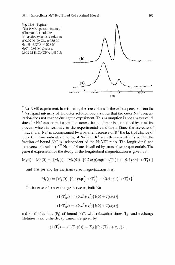
23Na-NMR experiment. In estimating the free volume in the cell suspension from the23Na signal intensity of the outer solution one assumes that the outer Na+ concen-tration does not change during the experiment. This assumption is not always valid.since the Na+ concentration gradient across the membrane is maintained by an activeprocess which is sensitive to the experimental conditions. Since the increase ofintracellular Na+ is accompanied by a parallel decrease of K+ the lack of change ofrelaxation time indicates binding of Na+ and K+ with the same affinity so that thefraction of bound Na+ is independent of the Na+/K+ ratio. The longitudinal andtransverse relaxation of 23 Na nuclei are described by sums of two exponentials. Thegeneral expression for the decay of the longitudinal magnetization is given by,

MzðtÞ �Mzð0Þ ¼ ½ðMzðtÞ �Mzð0ÞÞ�½f0:2 expðexpð�t=Tf1Þg þ f0:8 expð�t=Ts

1Þg�

and that for and for the transverse magnetization it is,

Mx tð Þ ¼ ½Mx 0ð Þ�½f0:6 exp �t=Tf2

� �

þ 0:4 exp �t=Ts2

� �� ��

In the case of, an exchange between, bulk Na+

ð1=TfB2Þ ¼ ½ð0:p2Þðv2ÞfJ 0ð Þ þ Jðx0Þg�

ð1=TfB2Þ ¼ ½ð0:p2Þðv2ÞfJ 0ð Þ þ Jðx0Þg�

and small fractions (Pi) of bound Na+, with relaxation times TB, and exchangelifetimes, sex, c the decay times, are given by

ð1=Tf1Þ ¼ ½ð1=T1 0ð ÞÞ� þ Rif½ðPi=ðTf

B1 þ sexcÞg�

Fig. 10.6 Typical23Na-NMR spectra obtainedof human (a) and dog(b) erythrocytes in a solutionof 0.02 M DyCl3, 0.056 MNa2 H2 EDTA. 0.028 MNaCl, 0.01 M glucose.0.002 M K3Co(CN)6 (pH 7.5)

10.4 Intracellular Na+ Red Blood Cells Animal Model 193

There are similar expressions for T1s, T2

f and T2s. Here T1(0) is the relaxation

time of Na+ in the bulk solution. The relaxation rates of the bound Na+ are,

ð1=TfB1Þ ¼ ½ð0:4p2Þðv2ÞfJðx0Þg�

ð1=TsB1Þ ¼ ½ð0:4p2Þðv2Þfð2x0Þg�

ð1=TfB2Þ ¼ ½ð0:p2Þðv2Þf 0ð Þ þ Jðx0Þg�

ð1=TsB2Þ ¼ ½ 0:2ð Þp2ðv2ÞfJðx0Þ þ Jð2x0Þg�

JðxÞ ¼ ½fsc=f1þ ðx2s2Þg�Here v = (e2qQ/h) is the quadrupolar coupling constant in Hz. For the inter-

pretation of the relaxation rates of intracellular Na+ it is convenient to divide thevarious contributing factors into three groups: (a) effect of viscosity on the rota-tional correlation time; (b) binding to small molecules: (c) binding to macro-molecules and membranes. Within the frequency range used, the condition (x0

sc) \\ 1 is expected to hold for the first two groups but not for the third. Since therotational correlation times of hydrated ions and their complexes with smallmolecules in aqueous solutions are in the range of *10-11 s, it is only when sc

changes by a factor of *100 that (x0 sc) becomes equal to 1.In the case of the third group of possible contributions to the relaxation rates i.e.,

binding of Na+ to macromolecules or membranes, the longitudinal relaxation time isexpected to be dependent on the frequency. Measurements of T1 of intracellular Na+

in the case of canine and human erythrocytes shows no such dependence at x0/2p; = 95.26. 79.38 and 23.81 MHz. These results indicate that T1 of intracellularNa+ is not affected by binding to macromolecules, but is determined by the viscosityof the intracellular medium or by binding to small molecules. However if this werethe only effect one would expect T1, to be equal to T2, The fact that the measured T2,of intracellular Na+ is significantly shorter than T1 clearly indicates an effect of Na+

binding to macromolecules or membranes on T2.On examination of the above equations one can see that in cases where T2 is

significantly shorter than T1 there are contributions from terms with (x0 sc) [ 1 andtherefore the two components of T2, should be significantly different and easilyseparable. It was noted T1, is not easily separable because its two components maydiffer by less than a factor of 4 and the fast relaxing component accounts for only20 % of the total intensity. However, in our system, an alternative explanation isprobably applicable. Since for the bound Na+. (x0 sc [[ 1), both J(x0) and J(2 x0)are very small and the effect of bound Na+ on T1 is negligible, i.e., T1

f = T1s = T1(0).

10.5 Triple Quantum Filtered NMR Animal Model

There is growing trend in research and development efforts to distinguish Na+ indifferent tissue compartments by the use of multiple-quantum (MQ) filters [5].23Na has a spin quantum number I = 3/2 and hence has four possible spin

194 10 Biomedical Diamagnetic Spin and Electric-Qudrupole Interaction Systems

orientations. This results in three possible single quantum (SQ) transitions, one,inner -1/2 to 1/2 transition and two outer -3/2 to -1/2 and +1/2 to 3/2 transitions.23Na is transiently bound to macromolecules. The electric field gradients created atthose sites act as an effective relaxation mechanism and the outer transitions relaxmore quickly than the inner transition. It has been shown that, when Na+ has twodistinct relaxation rates for the inner and outer transitions, the coherence transferselection rule, can be violated and, MQ transitions, become possible. Thus it wassuggested that the MQ-filtered signal should have large contribution from Nai

compared to Nae. It has been demonstrated that the following studies are veryuseful. (1) to measure the contributions of Nai

+ and Nae+ to the triple quantum (TQ)

23 Na signal from the in vivo rat liver, using TmDOTP5 (shift reagent) to lift thedegeneracy between the two signals, and (2) to compare changes in SQ (singlequantum) versus TQ (triple quantum) 23Na signals, during ischemia, produced bysacrificing the animals. SQ 23Na spectra, were collected using, a simple one pulsesequence with a 30 ls excitation pulse and a 10 ls spectrometer dead time, beforeacquisition.

TQ-filtered spectra were collected using the pulse sequence given asðhÞu � s=2� ððhÞu � ð2hÞuþp=2 � hÞuÞ � s=2� ðhÞuþp=2 � d� ðhÞp=2 � ðtacqÞ�.

Here h is a nominal 90� pulse, s is MQ preparation time, d is MQ evolution time,and tacq is acquisition time. A 48-step phase cycling scheme was used. The basicphase cycling scheme for selective detection of TQ coherence consisted of sixsteps in which the phase u = np/3, where n was cycled through 0,1,2,3,4, and 5.The FIDs resulting from this pulse sequence were alternately added to andsubtracted. Modulation of the TQ-filtered Na,+ signal, from liver, can be expres-sed, as a function of evolution time d, as I ¼ I0½cosð6pvd�½ exp�fðd=TTQÞg�: HereI = amplitude of the modulated signal, I0 = the amplitude of the same signalwhen d ¼ 0, v is the frequency offset in Hz, and TTQ is the TQ transverse

Fig. 10.7 TQ-filtered 23Na spectra from the in vivo rat liver, collected using a 3-ls b 315-ls,and c 630-ls evolution times. The modulation of the Nae

+ signal (5 ppm off resonance) indicatesthat it is a true TQ-filtered signal (5 ppm). Nex = external sodium, Nint = internal sodium

10.5 Triple Quantum Filtered NMR Animal Model 195

relaxation time. Thus, a true TQ-filtered signal would be modulated, such that it

would have maximum positive intensity at d = 0, be null at d ¼ 12mð Þ�1 and havemaximum negative intensity at S = (6v)-1.

The intensity of TQ-filtered signal depends upon the slow and fast transverserelaxation times. It is given as I = A [{exp (– s/T2f)} –{exp (– s/T2s)}] Here T2s isthe slow transverse relaxation time, T2f is the fast transverse relaxation time, andA is a constant related to the number of nuclei, that produce the TQ-filtered, Na+

signal and the line shape. The Fig. 10.7 (s[5]), presents illustration, of the use-fulness of the TQ filter technique, in separation of internal (Naint/Nai) and external(Naext/Nae) sodium signals, in a non invasive manner. It shows that, the Nae

resonance, is modulating, as a function of, d. There is positive maximum, inintensity, at d = 3 ls, zero intensity at d = 315 ls, and a negative maximum atd = 630 ls. Therefore, the external sodium signal, can be manipulated, inde-pendent, of the internal sodium. The two signals appear at different resonancefrequencies. Once separated, the fast (internal) and slow (external) relaxation timeanalysis can be accurately performed. It is also seen, that the overall intensity, ofthe intra and extra cellular, Na+, resonances, decrease with increasing d. It is, dueto, the TQ/T2 relaxation, during the d delay.

References

1. Forsfin, S., Drakenbergj, T., Wennerstrom, H.: NMR studies of ion binding in biologicalsystems. Q. Rev. Biophys. 19(1/2), 83–114 (1987)

2. Tanase, C., Boada, F.E.: Algebraic description of spin 3/2 dynamics in NMR experiments.J. Magn. Reson. 173, 236–253 (2005)

3. Choy, J., Ling, W., Jerschow, A.: Selective detection of ordered sodium signals via the centraltransition. J. Magn. Reson. 180, 105–109 (2006)

4. Shinar, H., Navon, G.: NMR relaxation studies of intracellular Na+ in red blood cells. Biophys.Chem. 20, 275–283 (1984)

5. Seshan, V., Sherry, A.D., Bansal, N.: Evaluation of triple quantum-filtered 23Na NMRspectroscopy in the in Sifu rat liver. Magn. Reson. Med. 38, 821–827 (1997)

196 10 Biomedical Diamagnetic Spin and Electric-Qudrupole Interaction Systems

Chapter 11Practical Illustrations SodiumSpectroscopy and Imaging: ClinicalApplications

11.1 Vasogenic Edema: Experimental Canine/Human Model

A valid distinction between cytotoxic and vasogenic edema [1] is based mainly onthe differences in blood–brain barmier permeability. Vasogenic edema fluiddevelops in association with a variety of pathologic conditions such as brain tumors,brain abscesses hypertension or areas of infarction. In cases of brain tumor edemafluid leaks from the tumor vessels and spreads into the surrounding white matter.Similarly, cryogenic injury of the cerebral cortex causes a transient breakdown of theblood–brain barrier in the zone bordering the necrotic region allowing edema fluid tospread into the white matter. The regions in which the blood–brain barrier isdefective and those in which the edema accumulates do not necessarily correspond.MRI has a proved to be a valuable and sensitive method by which to detect vasogenicedema. Multinuclear MR imaging (proton and sodium) permits in vivo assessmentof the relative distributions of water and sodium within the brain. One can define thesodium signal associated with edema fluid as well as investigate the relaxationcharacteristics of extra-cellular sodium, for properties that may be specific to sodiumin the extra-cellular compartment. A model of vasogenic edema can thus bedeveloped. Previously models have relied on local injury to the brain by either coldor chemical insult. The resulting region of necrotic brain has a defective blood–brainbarrier and vasogenic edema forms adjacent to the injured tissue. One can avoid amixture of necrotic and edematous brain tissue by the use of a non traumatic mode ofvasogenic edema in mongrel dogs.

A major technical obstacle is catheterization of the internal carotid artery withoutinducing spasm. This was accomplished by gently placing the catheter tip into theinfundibulum of the internal carotid artery and making a test injection. The majorarterial supply to the canine brain is through the anastomotic ramus that originatesfrom the internal maxillary artery and joins the internal carotid artery. Thereforeocclusion of the internal carotid artery by the catheter tip does not produce ischemia.However spasm of the internal carotid artery results in adequate delivery of osmotic

M. M. Kaila and R. Kaila, Molecular Imaging of the Brain,Series in BioEngineering, DOI: 10.1007/978-3-642-30302-9_11,� Springer-Verlag Berlin Heidelberg 2013

197

agents to the cerebral hemisphere and failure to disrupt the blood–brain barrier. Theproton images of the two patients (chronic/human) with vasogenic edema secondaryto well-circumscribed meningiomas revealed reduced signal intensity on the mul-tiple saturation recovery images at TRs of 150 and 300 ms. The calculated T1 imagesgave poor definition of the region of edema. On the third- and fourth-echo MSE(multi-spin echo) images as well as the calculated T2 images the areas of vasogenicedema were well circumscribed and easily discernible. The sodium images of thesepatients revealed an increased sodium signal from the regions of vasogenic edema.The sodium signal was very intense and easily identified. In the normal brainelectron microscopy demonstrates substantial variation in the extra-cellular com-partment. In the gray matter the cellular membranes are in a regular pattern and areseparated by only 100–200 angstroms (*10 nm) whereas in the white matter theintracellular spaces are irregular and may be oven 800 (*80 nm) angstroms wide. Inthe white matter, edema causes widening of the extra-cellular spaces and swelling ofastro-cystic processes. In vasogenic edema the excess extra-cellular fluid is relatedto increased permeability of the blood–brain barrier such as occurs in the vicinity ofbrain tumors traumatic lesions and inflammatory foci. The increased vascular per-meability allows indiscriminate escape of plasma components including serumproteins, electrolytes, and water.

The events that lead to the formation of vasogenic edema are not simultaneous.When the blood–brain barrier is opened through acute injury water and electrolytesfirst enter the extra-cellular space. The sodium content of vasogenic edema fluidinduced by cryogenic injury increases. The spread of extravasated plasma contents(water, sodium and plasma proteins) is much more extensive in the white matter thanin the gray matter. Also the osmotic pressure of the edema fluid colloid is elevated inaccordance with its high protein content. The force that propagates vasogenic edemaappears to be the mean arterial blood pressure which subsequently is influenced bythe state of cerebral vasomotor autoregulation. Increased blood–brain barriers per-meability effectively makes edematous brain tissue part of the extracerebral sys-temic extnacellu!ar space and therefore liable to expansion and nonosmotichyperhydration. Similarly, the defective blood–brain barrier allows rapid penetra-tion of osmotic agents into the affected areas. This accounts for the poor response ofvasogenic edema to systemically administered osmotic agents. The characterizationof sodium in the extracellular compartment by MR imaging is complicated by thequadrupolar nature of the sodium nucleus. The quadnupolar relaxation of a spin 3/2nucleus decays as a weighted sum of two exponentials. The result is a two-com-ponent T2 relaxation. Vasogenic edema fluid corresponds best to a two-siteexchange model. In such a model the sodium ion exchanges between a solvated freestate and a bound site on a serum macromolecule. Sodium ions tightly bound toserum proteins will not contribute to the total intensity of the sodium signal.

It is demonstrated that approximately 1 % of serum sodium is bound and that itis in constant fast exchange between potential binding sites on serum macro-molecules and aqueous solution. It is seen there is shortened T2 values for serumsodium compared with those of sodium bromide solutions. This effect was notattributed to protein binding but rather to the presence in serum of polyelectrolytes

198 11 Practical Illustrations Sodium Spectroscopy and Imaging: Clinical Applications

that are surrounded by ordered shells of water molecules, a configuration thatincreases the reorientation time of both water molecules and hydrated ions. In vivosodium MR imaging provides an opportunity to study the electrolyte compositionof edema fluid. Current imaging techniques enable in vivo measurement of the twomajor components of edema fluid: water and sodium. Water content is assessed byinvestigation of the proton density, T1, and T2. Sodium content is assessed bysignal intensity and T2 relaxation characteristics. One hopes in the near future to beable to quantitate the sodium signal and thus provide an opportunity to investigatetissue osmolality. Sodium MR imaging offers the potential for providing newinsights into the management of patients with vasogenic edema and may alsopermit in vivo estimation of the abnormalities, in extra cellular space associatedwith cerebral neoplasm. In the Fig. 11.1 are presented clinical results in the humanmodel.

11.2 Tissue Sodium Concentration Tissue Viability (Stroke):Human Model (Conventional MRI)

It is imporatnat in some situations to know the role of sodium MR imaging in acomprehensive MR imaging protocol for monitoring tissue viability [2] in stroke.One can use for this purpose TSC (tissue sodium concentration) as measured bysodium MR imaging with apparent diffusion coefficient (ADC) and blood poolparameters derived from proton MR imaging. It can be done in a nonhumanprimate model of acute embolic stroke and in patients with acute or nonacutestroke. The TSC parameter was evaluated in the setting of stroke along with thediffusion and perfusion parameters. Representative images and maps for a 62-year-old man with a 1-day-old stroke are presented in Fig. 11.2 [4]. It demonstrates theresults from the comprehensive MR imaging protocol. In the area of stroke thethrombus caused the bolus of contrast material to have a prolonged TTT (tissuetransit time) and delayed TA (arival time). These were displayed as bright voxels.Conventional 1H MR imaging is insensitive for the detection of acute stroke.Diffusion-weighted imaging and its quantitative counterpart of ADC mapping arevery sensitive in the early detection of ischemia. ADC and diffusion-weightedimaging show changes well before the thresholds of irreversible tissue injuryrelated to water and ion homeostasis. The ADC and diffusion-weighted imagingare sensitive for detection of ischemia but do not provide a complete description ofpathophysiologic conditions due to stroke in the primate brain. For any particularset of MR images to be useful in a clinical setting, particularly in a medicallyurgent situation such as acute stroke the technical success rate for yielding usefulinformation must be considered.

Sodium MR imaging has long been proposed as a useful method to assesspathologic changes in the brain but medical applications have not developed becauseof the lack of an acceptable clinical implementation. The potential benefits of this

11.1 Vasogenic Edema: Experimental Canine/Human Model 199

method in stroke have been overshadowed by the newer proton-based methods ofdiffusion and perfusion imaging. Whereas the ADC parameter was useful indetecting the stroke very rapidly after embolization it was less informative over thecritical first 6 h as it remained relatively stable. In marked contrast TSC (tissuesodium concentration) showed a linear increase over 6 h characterized by a rate ofincrease of about 5.7 mmol/L/h and approached 70 mmol/L at 6 h by which time the

Fig. 11.1 a Contrast-enhanced axial CT scan of a patient with a flax meningioma. b CoronalMSE image (TR 600 ms) obtained along the posterior margin of the meningioma. The vasogenicedema is inconspicuous. c Calculated T1 image (long T1 represented as high intensity) poorlydefines the edematous region. d Coronal image obtained with a MSE sequence (TE 100 ms,TR = 2,000). The edematous area is well delineated. e Calculated T2 image also demonstratesthe edematous white matter clearly f, g Coronal sodium MR images at TE 13, 26, and 39 ms. Thesodium signal intensity is markedly elevated in the region of vasogenic edema. g Coronal sodiumimages (TE 13, 26, and 39 ms) that include areas of normal brain tissue, vasogenic edema, andcerebrospinal fluid (CSF) in the occipital horn. The sodium signal in the edema fluid appears tohave a slightly shortened T2 than in the CSF

200 11 Practical Illustrations Sodium Spectroscopy and Imaging: Clinical Applications

tissue was shown at histologic examination to be infarcted. The progression of stroketo infarction is dependent on both perfusion level and duration of reduced flow. Thesteadily increasing TSC level marked the changing metabolic status of the lesion. Asshown in the treated animal, thrombolytic therapy after 150 min when TSC was stillbe (low 55 mmo/L) markedly decreased the volume of the infarct as compared withthe result with no intervention.

As new neuroprotective agents enter clinical practice as alternatives tothrombolysis triaging patients to undergo appropriate therapies may be helped bythis comprehensive MR imaging assessment of the tissue physiologic conditionand viability. The model of TSC for assessing hyperacute stroke physiology isdescribed approximately as follows. Table 11.1 [2] shows the scheme that sum-marizes the relationship between TSC and loss of tissue viability for a two-compartment model in which the vascular and extracellular compartments are

Fig. 11.2 Representative MR images in a 62-year-old man who presented with left-sidedparalysis that lasted 24 h. a T2-weighted spin-echo 1H image (2,500/102) through a stroke lesion(arrow). b 23Na image (80/0.4). C Diffusion-weighted 1H image (6,000/152). d ADC map.e Relative CBV map. f TTT map. g TA map. Parameter values for the lesion and the contralateralnormal region respectively are as follows: TSC, 78 and 46 mmol/L; ADC, 0.21 9 10-3 and0.64 9 10-3 mm2/sec; TTT (tissue transit time), 37 and 14 s; and TA, 16 and 11 s. The relativeCBV (cerebral blood volume) of the lesion was just less than half that of the contralateralhomologous region

Table 11.1 Vasucular Compartment (3 % Na)

Vascular Compartment (3 % Na) = 140 mM

Intra-cellular Compartment(85 %)Na = 10 mM

Extra-cellular Comprtment(12 %)Na = 140 mM

11.2 Tissue Sodium Concentration Tissue Viability (Stroke): Human Model 201

considered as one compartment. For an intracellular compartment volume Vi andsodium concentration Ci and an extracellular compartment volume Ve, and sodiumconcentration Ce, the conservation of mass gives the following: TSC(Vi ? Ve) = VeCe ? ViCi. For a voxel of volume V, V = Vi ? Ve or Ve = V - Vi,which allows, TSC to be expressed in terms of the intracellular volume fraction Vi/V, as follows: TSC = Ce ? (Ci – Ce) (Vi/V). Thus for a fixed volume fractionincreasing intracellular sodium concentration Ci increases TSC. Alternatively asthe intracellular volume fraction decreases with loss of cell integrity TSCapproaches Ce. It is important to realize this model is not just a redistribution ofsodium within a voxel. The extracellular compartment is buffered with evenminimal perfusion and the high diffusibility of sodium ions from the space of theentire body which is regulated systemically at a constant value of Ce.

It represents diagram of the two-compartment model of TSC. The vascularcompartment is a part of the extracellular compartment as the extracellular sodiumconcentration (in millimoles per liter) is always maintained because of the rapiddiffusion of sodium ions from the vascular compartment that is buffered by the restof the body. In normal brain tissue the large intracellular compartment maintains alow sodium concentration against a high sodium concentration in the smallextracellular compartment. During stroke the normal intracellular space decreasesand the extracellular compartment expands with loss of ion homeostasis as the cellintegrity is lost. As the extracellular sodium concentration is maintained throughthe vascular compartment even at low levels of perfusion, TSC must increase,which is a direct measure of the loss of cell integrity. Percentages in parenthesesare percentages of voxel volume (Table 11.2) [4].

It represents diagram of the two-compartment model of TSC. The vascularcompartment is a part of the extracellular compartment as the extracellular sodiumconcentration (in millimoles per liter) is always maintained because of the rapiddiffusion of sodium ions from the vascular compartment that is buffered by the rest.

11.3 Human Brain In-vivo Sodium MRI: Soft InversionRecovery (Conventional Versus Quantum MRI)

The ability to assess intracellular sodium concentrations [Nain] may greatlyfacilitate the diagnosis of diseased tissue in the human brain [3]. [Nain] appears todirectly correlate with the rate of cell proliferation and monitoring [Nain] may be

Table 11.2 Vasucualr Compartment (4 %)

Vascular Compartment (4 % Na) = 140 mM

Intra-cellular Compartment(Intact)[Na] = 10 mM

Intra-cellular Compartment(loss of ion homeostasis)[Na][ 10 mM

ExtracellularCompartment[Expanding][Na] = 140 mM

202 11 Practical Illustrations Sodium Spectroscopy and Imaging: Clinical Applications

useful in the analysis of neoplasms and their response to chemotherapy. The abilityto assess [Nain] may also be useful in the setting of acute stroke as dramaticallyincreased [Nain] levels associated with anoxic depolarization and the subsequentrelatively slow diffusion of sodium ions from other parts of the brain into theischemic core appear to be directly linked to cell damage during ischemia. Thevaluable information pertaining to the diseased state of tissue can be obtained withsodium MRI techniques that facilitate quantification of bulk tissue sodium con-centrations; strongly intracellular weighted imaging techniques that limit thesignal contribution from the more highly concentrated extra-cellular space (ECS)(140 mM vs. 10–15 mM intracellular) may provide an improved means to char-acterize [Nain] in some cases. There is an approach to use of multiple-quantumfiltering techniques. However, the signal intensity following a multiple-quantumspin sequence is a small fraction of the signal intensity following a single ideal 90o

excitation pulse (10 % has been given as a typical in vivo value). There is ananother approach that uses. an inversion recovery (IR) Technique. A considerableT1 relaxation differences exist between two environments. IR can be used toeliminate the signal contribution from either environment. Although it is wellunderstood that the ECS (extra-cellular space) in the brain contains many differenttypes of proteoglycans most attached to the cell membranes little is known aboutthe density of these molecules.

It has been suggested that the density of this extra-cellular matrix is quite sparseallowing volume transmission through the ECS. Because T1 measurements havebeen shown to correlate with matrix density, sodium T1 relaxation in the ECS maybe significantly longer than in the intracellular space (ICS). Shift reagent aidedexperiments using an implanted gliosarcoma in rats also suggest this to be the case.Minimal sodium exchange is expected between the ICS and ECS on the relevantsodium NMR timescale. If the sodium T1 in the ECS is significantly longer than inthe ICS an IR sequence may be used to eliminate the ECS signal contribution from asodium image. When the relaxation constants T1 and T2 are much longer than an RFpulse the effects of relaxation during the pulse can essentially be ignored. Thecalculation of flip angle is simple and is directly related to pulse power and length.While this is usually the case for the uncoupled 1H nuclide this is not the case for thequadrupolar sodium nucleus. An IR technique labeled soft inversion recovery fluidattenuation (SIRFLA) is proposed for sodium imaging of in vivo human brain. Theefficacy of this technique is demonstrated through the minimization of sodiumsignal from the cerebrospinal fluid (CSF) brain images acquired at a static magneticfield strength of 4.7 T. The effectiveness of soft inversion pulses to separate sodiumlongitudinal magnetization in different environments has been shown analyzedalong with the resultant benefit in the SIRFLA sequence. This separation is thedirect result of the large quadrupole interaction experienced by the sodium nucleusand is not possible in conventional 1H NMR. It is because the inversion pulse lengthhas a dramatic impact on signal acquired from the non-nulled environment.

The IR sequence implemented with long RF inversion pulses has been given thenew designation SIRFLA. Considering the relaxation parameters the SIRFLAsequence may offer an SNR benefit over triple quantum filters (TQF) for

11.3 Human Brain In-vivo Sodium MRI: Soft Inversion Recovery 203

intracellular imaging. The TQF sequence is also limited by SAR as three hard 90�

RF pulses are required and increasing the RF pulse length decreases acquiredsignal intensity. A TQF sequence with three 1-ms 90� RF pulses and the same TRrepetition time) presented for the SIRFLA sequence would dissipate twice thepower of the SIRFLA sequence. The SIRFLA sequence can also theoreticallyfacilitate ‘‘full elimination’’ of the ECS signal contribution. In vivo TQF studiessuggest a 40 % residual contribution from the ECS. Several marked artifactualhyper intensities can be seen in Fig. 11.3a [3] that are not apparent in Fig. 11.3b[3]. The most significant affect begins above the sphenoid sinus and extends intothe frontal lobe. Two other less pronounced artifacts exist on the outer edges of theparietal lobes. Susceptibility induced B0 inhomogeneities are well known to existin these areas, a product of the surrounding sinuses and bone. Artifacts caused bythese B0 inhomogeneities are apparent in other imaging modalities such as single-shot EPI. These artifacts Fig. 11.3 a [3] are the result of the narrow bandwidthassociated with the long inversion pulse and are minimized by the wider band-width of the short inversion pulse in Fig. 11.3 b [3].

11.4 Statistically Optimal MRI Acquisition (General)

An exponentially decaying signal can be described by two parameters, itsamplitude q and decay rate k, given as [4] S(t) = [q (e-kt)]. Here t is the user-controlled encoding parameter (diffusion weighting or echo time). At least twomeasurements with different encodings e.g. t1 and t2 [ t1, are needed to estimate k.It has been shown that within all such ‘two point’ schemes the imaging time isused most efficiently when (t2 - t1) is chosen to be about 1.29/k. One can examinewhether multipoint acquisitions with several (more than two) encodings may bemore efficient than two-point schemes in the same total measurement duration.One routinely uses the v2-statistical fitting procedure as a measure of the precisionof the decay rate estimation. It demonstrates that the most efficient multipointscheme in fact approaches that of the two-point method. The optimal acquisitionstrategy is specified by a set of ti’s yielding the highest precision in the determi-nation of the decay rate. It is naturally with the smallest rk

2 i.e., the variance. Theexpression in general for the variance Ai, in terms of the optimum variance r0, canbe written as Ai ¼ ð1=r0Þ½ðe�kt

i Þ � tiqðe�kti Þ�. One performs this optimization in

the vicinity of the expected decay value, k = ktune, and then evaluate rk at arbi-trary k’s. If the actual value of k deviates from ktune, the precision degrades asshown in Fig. 11.4 [5]. The precision loss seen is only 15 % over a wide rangek * (0.6, 1.5) ktune. If the decay constants to be measured are expected to vary bymuch more than a factor of 1.5/0.6 = 2.5 the two-point method will be inefficientat the edges of the range of k’s.

Measurement of exponential relaxation constants for which the two-pointmethod is found to be the most efficient should not to be confused with thevalidation of the model of exponential signal decay. The latter is characterized by

204 11 Practical Illustrations Sodium Spectroscopy and Imaging: Clinical Applications

the goodness of the fit and requires acquisitions at multiple distinct encodings ti.Being optimal the two-point scheme lends itself admirably to applications relyingon measurement of the change in the relaxation constants such as micro vesseldensity estimation. Indeed images acquired before and after the relaxation con-stant. is altered say by administration of a contrast agent naturally constitute the

two points. Image intensity of the first point is given by ½qfeð�ktÞ0 g� while of the

second by ½qeð�ktÞ0 �½qfeð�MktÞg�. Since modification of the encoding parameter t

between the points introduces unwanted sensitivity to the unknown ‘‘resting’’tissue relaxation constant, k0, t has to be common to both acquisitions.

Fig. 11.3 a SIRFLA images acquired in healthy volunteer (inversion pulse length of 10 ms).SNR in the CSF is 4 and SNR in the brain tissue is 17. b Sodium IR images acquired with a muchshorter inversion pulse length of 1 ms and a TR of 334 ms. SAR and voxel size are equivalent toa and the image duration was 10.7 min (or *25 s shorter than (a)). SNR in the CSF is 2.5 andSNR in the brain tissue is 10. The SNR is 70 % greater in (a) with the longer inversion pulse thanin (b). One disadvantage of the longer inversion pulse is its narrow bandwidth which results in anartifactual hyper intensity in the known areas of susceptibility a that is not seen in b. The imagesin (a) and (b) are not globally scaled

11.4 Statistically Optimal MRI Acquisition (General) 205

The optimal acquisition strategy consists of choosing the value of t to yield the

highest precision of Dk. Interpreting ½qfeð�ktÞ0 g� as the amplitude of the decay q

and Dk as decay constant, k casts the problem, in terms of the relaxation constantestimation considered with one exception; q depends on the user selectableparameter t. However, in applications such as microvasculature imaging, requiringhigh doses of contrast agents k0 is much smaller than Dk. Therefore, for optimi-zation purposes in the vicinity of Dk the t dependence of q can be neglected. Thus,optimal exponential weighting, t as well as relaxation constant alternation arefound by replacing ktune with Dk. Figure 11.4 [4] represents summary of thegraphical picture of the analysis.

11.5 Spin 3/2 Bi-Exponential Relaxation Multi-QuantumFiltration Technique (23Na Spectroscopy)

It is known that metal ions play a vital mediating role in many important biologicalprocesses. As a result of their relatively favorable properties NMR studies of thespin-3/2 nuclei, 7Li, 39K, 87Rb, and, most frequently 23Na have proved popular.The two main areas of interest [5] have been the study of these nuclei in

Fig. 11.4 Precision as a function of k for several N-point protocols tuned for ktune. Here the SNR isthe signal-to-noise ratio of the average of N images with minimal exponential weighting and ingeneral, is a function of k, if the minimal weighting, is not zero. Note that the precision of protocolswith N C 3 is already very close to optimal. Since the convexity of the curves is very small theprecision stays within. 15 % of the best over a broad interval (0.6, 1.5) ktune. As an example of acommonly used scheme the precision for optimal 6-equally-spaced-point protocol is superposed

206 11 Practical Illustrations Sodium Spectroscopy and Imaging: Clinical Applications

intracellular environments and of their binding to biological molecules in solution.In both cases the spin-3/2 nuclei are likely to be tumbling in the slow-motionregime i.e. possessing a rotational correlation time s comparable to the inverse ofthe Larmor frequency xo and it is known that under these conditions both thetransverse and the longitudinal quadrupolar relaxation are biexponential. Often,however biexponential relaxation is difficult to distinguish from simple expo-nential relaxation using conventional NMR methods. Recently it has been shownthat biexponentially relaxing spin-3/2 nuclei can be filtered through a state ofmultiple-quantum coherence. Multiple-quantum filtration techniques can thereforeprovide unambiguous evidence of the presence of biexponential relaxation. In thisfashion intracellular and extra cellular metal ions can be distinguished since thelatter are almost always in the fast-motion regime (where they exhibit simpleexponential relaxation) and the NMR signal from these ions will not pass the filter.The lineshape resulting from multiple-quantum filtration consists of the differenceof two Lorentzians and analysis of this highly characteristic line shape in bindingstudies can indicate the motional and exchange behavior of the metal ions. In allstudies of this type sensitivity is usually a prime concern because of the lowconcentration of metal ions in the slow-motion regime.

It has been demonstrated that a double-quantum filtration experiment for thedetection of biexponential transverse relaxation in spin-3/2 nuclei works well.Some workers have apparently without exception adopted the double-quantumfiltration techniques. Others also used a triple-quantum filtration experiment forthe detection of bi-exponential longitudinal relaxation. It can all be done withgreater sensitivity using triple-quantum filtration than using double-quantum fil-tration techniques. The signal amplitudes produced by the double- and triple-quantum filtration techniques for spin-3/2 nuclei are conveniently calculated usingan irreducible tensor operator formalism. The density operator r(t) for an isolatedspin of quantum number S is expanded in the form r (t) = Rl=0 to 2s R p=-1 to l

Clp(t)Tlp, Here Tlp is an irreducible tensor operator of rank l and coherence order p.The matrix representations for S = 3/2 can be found in the MRI literature.

The transformation of an operator Tlp under a radiofrequency pulse of flip angleb, and phase u, is given in the familiar ‘‘arrow notation’’ by Tlp - b (Iy cos u – Ix

sin u) ? Rp0Tlp0 dlp0

p0(b) exp{-i Dp u)}, where p0 is the new coherence order, andAp = p0 - p is the change in coherence order under the pulse. The amplitude ofthe transfer Tip to Tip0, is given by the reduced rotation matrix element dlp0p(b). Byconvention the dlp0p(b) are defined so that the phase u represents a positiveexcursion with respect to the rotating frame y axis (i.e., u = 0 for a y pulse,u = 90� for a –x pulse, and so on). The rank 1 of a tensor may change under freeprecession or relaxation but this evolution is the same in both double and triple-quantum filtration experiments and has been calculated in detail. The pulsesequence and coherence transfer pathway diagram for multiple-quantum filtrationof spin-3/2 nuclei exhibiting biexponential transverse relaxation are shown inFig. 11.5 [5]. Significant transverse relaxation takes place during the evolutionperiod se and the acquisition period t2 but not during sm. The phase angle u0 is 0�for excitation of double-quantum coherence (dotted coherence transfer pathways)

11.5 Spin 3/2 Bi-Exponential Relaxation Multi-Quantum Filtration Technique 207

and 90� for triple-quantum coherence (solid pathways) while the phase u and thereceiver are phase cycled to select the desired pathway.

The phase u0 in (a) is 0� for double quantum and 90� for triple quantumfiltration. Maximum sensitivity is achieved with flip angles b = b0 = 90�, exceptfor the double quantum filtration version of (b) where b = 54.7�. To study biex-ponential longitudinal relaxation a variable evolution period t must be used in (b)rather than a fixed evolution period se. The period sm, is typically a few micro-seconds to allow for phase shifting of the pulses. From the form of the third-rankreduced rotation matrix elements d3p0p(b) it can be shown that the signal ampli-tude from both techniques is maximum if the flip angles b and b’ of the two pulsesin the filter are both 90�. With b0 = 90� the amplitude of coherence transferthrough p = ? 2 (or +3) is the same as that through p = -2 (or -3). Using theoptimum phase cycling of the phase u and the receiver the relative signalamplitudes from the double- and triple quantum filtration experiments can bedetermined from STQF/SDQF *1.5 (mono-exponential case), *1.3 (bi-exponentialcase). One can mathematically calculate relative signal amplitudes produced bythe transverse and longitudinal experiments as function of x0sc (x0 = LarmorFrequency, sc = correlation constant and is plotted in Fig. 11.6 [5].

Fig. 11.5 Pulse sequences and coherence transfer pathway diagrams for multiple quantumfiltration of spin-3/2 nuclei. The ‘‘transverse experiment’’ (a) is used to study biexponentialtransverse relaxation and the ‘‘longitudinal experiment’’ (b) is used to study longitudinalrelaxation. The phase u in (a) and (b) is stepped through the values 0�, 90�, 180�, and 270� fordouble-quantum filtration (dotted coherence transfer pathways) and through 30�, 90�, 150�, 2 l0�,270� and 330� for triple-quantum filtration (solid pathways), while the receiver phase is alternatedbetween 0� and 180�

208 11 Practical Illustrations Sodium Spectroscopy and Imaging: Clinical Applications

11.6 Sodium Twisted Projection Imaging (TPI)/ConventionalMRI (ADC Maps) Human Model

Regulation of sodium homeostasis through counter-balancing low intracellular andhigh extra cellular sodium ion concentrations with potassium ions is of vitalimportance for cellular function [6] These ion gradients across the cell membraneprovide the potential energy for many important cellular transport processes.Action potentials intracellular pH regulation and many membrane transport pro-cesses are all directly dependent on the sodium ion gradient across the cellmembrane. Damage to brain cell integrity and disruption of cell packing producelocal increases in tissue sodium concentration (TSC). TSC determined by quan-titative MRI has been shown to have a potential role in monitoring tissue viabilityin humans with diseases such as stroke and in monitoring treatment of braintumors. Despite these potential medical applications described more than twodecades ago quantitative sodium imaging has been slow to evolve.

The sodium MR signal has a detection sensitivity of four orders of magnitudelower than that of the proton signal. It exhibits biexponential relaxation behaviorwith fast and slow transverse relaxation characteristics (T2

fast, 1–3 ms and T2slow,

12–25 ms, respectively) in biologic tissues. Therefore, sodium imaging requires animaging sequence with a short excitation radiofrequency (RF) pulse and a shortecho time (TE) to reduce signal loss from the rapid decay of the transversemagnetization. Twisted projection imaging (TPI) is a three-dimensional (3D)projection reconstruction sequence–based approach that can achieve short TEvalues and high acquisition efficiency.

When performed at long pulse repetition times to allow full T1 relaxationquantification of TSC is possible. However the generation of TPI [6] gradient

Fig. 11.6 Ratio of the signal amplitude from the optimized transverse experiment to that fromthe longitudinal experiment as a function of x0 sc (x0 = Larmor Frequency, sc = correlationconstant) for pure quadrupolar relaxation. The optimum fixed evolution periods se have been usedat each value of x0sc. The signal amplitude from the transverse triple-quantum filtrationexperiment is half that from the longitudinal experiment for x0sc but is 1.59 times greater in thelimit of infinitely large x0sc

11.6 Sodium Twisted Projection Imaging (TPI)/Conventional MRI (ADC Maps) 209

waveforms is often limited by the hardware slew rate constraint especially whenstarting twisting at low k-space radius is desired to reduce the number of pro-jections needed to sample k-space at the Nyquist rate. Besides being potentiallyharmful to the subject and the gradient system violations of the slew rate constraintcan also cause uncertainty in the k-space trajectory. The slew rate constraint can bemet by using low gradient amplitude or numerical smoothing. However, theseapproaches result in either a long readout time that ultimately limits the achievablespatial resolution due to T2 relaxation, or k-space trajectory deviations thatdegrade the point-spread function (PSF) of the sequence. Meanwhile, the high dataacquisition efficiency of TPI stems from its ability to sample more k-space loca-tions in each repetition, with a relatively long readout window. This renders TPIsensitive to static field (B0) inhomogeneity even at the relatively low sodiumresonance frequency. These B0 inhomogeneities must be corrected to avoid sig-nificant image blurring and distortion. In the Fig. 11.7 [6] and 11.8 [6] one wouldfind a practical illustration of the results obtained by the TPI technique.

11.7 Human Brain: Diffusion Weighted Magnetic ResonanceSpectroscopy (MRS) And Imaging (Conventional MRI)

Magnetic resonance is well established for measuring the diffusion properties ofwater in the human brain and it has been proven to be useful in numerous neu-rological disorders. Diffusion-weighted imaging (DWI) of tissue water includescontributions from exchanging intra- and extra cellular water, which makes

Fig. 11.7 Representative TSC maps a obtained on a healthy volunteer (unit: millimoles/litertissue). The corresponding T1-weighted proton images are also shown b as anatomic references.The TSC images shown are before water fraction correction. The WM (white matter) ispredominantly shown and also the GM (Grey matter) is recognized between cerebrospinal fluid(partial-volume effects with brain parenchyma) and WM

210 11 Practical Illustrations Sodium Spectroscopy and Imaging: Clinical Applications

compartment-specific interpretation of diffusion characteristics rather complex.The diffusion characteristics of intracellular metabolites can be measured byincorporating diffusion sensitizing gradients with spatial localization in a spec-troscopy pulse sequence, i.e., diffusion-weighted magnetic resonance spectroscopy(DW-MRS) [7]. The main research focus of DW-MRS thus far has been on animalmodels of cerebral ischemia in which the apparent diffusion coefficients (ADCs) ofthe singlet metabolites are reduced significantly in the acute phase of cerebralischemia, similar to the ADC reduction of water. These studies indicate that dif-fusion changes of metabolites may be useful in probing the effect of stroke andother pathologies on the intracellular environment. There have been some studieson the diffusion characteristics of the metabolites N-acetyl aspartate (NAA), cre-atine and phosphocreatine (tCr), and choline (Cho) in the human brain.

There are problems with measuring the ADC (apparent diffusion coefficient) ofthe metabolites, including low concentration, small ADCs, and macroscopicmotion due to involuntary subject movements, respiration, and cerebrospinal fluidrelated brain pulsations. These motion errors cause a decrease in the signalintensity of the metabolite peaks which in turn results in an apparent increase inthe measured ADC. It was proposed a phase error correction method using theresidual water peak as well as cardiac gating for correction of the motion-inducederrors. These methods were applied and reported that the ADCs of NAA, tCr, andCho were found to decrease in acute stroke and increase in the peripheral region ofa tumor including edema. It was suggested that since NAA is a neuronal markerthe ADC differences are an indication of neuronal cell viscosity changes as a result

Fig. 11.8 Axial B0 field maps are shown for a normal volunteer using a sodium imaging in4 min and b proton imaging in less than 2 min. These B0 maps were applied to c the uncorrectedimages to derive d human images corrected using sodium B0 field maps, and e human imagescorrected using proton B0 field maps. The improvements appreciated in the brainstem (whitearrows) are similar for both sodium and proton

11.7 Human Brain: Diffusion Weighted Magnetic Resonance Spectroscopy 211

of the pathologic status of the tissue. The micro structural organization of whitematter in brain tissue leads to directional dependence (i.e., anisotropy) of the ADCof water, and presumably of the metabolites as well. However, the trace/3 (X, Y,Z), ADC provides a rotationally invariant measure of molecular diffusion in tissue.Some previous human studies examined the ADC of NAA, tCr, and Cho in sub-cortical white matter of human brain but the diffusion was only measured in onearbitrary direction. Therefore the purpose of this study is to quantify the rota-tionally invariant trace/3 ADC values of the metabolites NAA, tCr, and Cho invarious regions of the healthy human brain. A new phase correction method isproposed for processing the diffusion-weighted spectra. The Fig. 11.9 [7], and the

Fig. 11.9 Spectra at low andhigh b (apparent diffusioncoefficient) values with thediffusion gradient applied inthe Y (anterior–posterior)direction in a subcorticalwhite matter (SWM)b occipital gray matter(OGM), and (c) frontal graymatter (FGM). The signalintensity of the NAA peakdropped 17, 20, and 24 % athigher b values in the SWM,OGM, and FGM regions,respectively

212 11 Practical Illustrations Sodium Spectroscopy and Imaging: Clinical Applications

Table [7] present details about a practical illustration of diffusion weighted MRI oftissue structure in human brain (Table 11.3) [7].

11.8 Human Brain Metabolites: Proton T1 and T2 RelaxationTimes (Conventional MRI)

Reasonable estimates of relaxation times of brain metabolites are important foraccurate quantitation of MR spectra, for optimizing measurement protocols, forabsolute quantitation in single voxel MR spectroscopy and in quantitative spec-troscopic imaging. Relaxation times of metabolites in proton MR spectra of humanbrain in vivo have been the subject of studies for 3T(Tesla) [8]. Both longitudinaland transverse relaxation times of brain metabolites should follow relaxationdispersion of water protons, experiencing similar longitudinal relaxation mecha-nisms. Correspondingly, the T1 values should increase and the T2 values shoulddecrease with increasing static magnetic field B0. The decrease in T2 for N-acetylaspartate, creatine and choline compared to the lower field data has alreadybeen reported at 4.1 and at 4T. Accuracy of the obtained relaxation times isaffected by several factors. A proton spectrum of the brain in vivo represents asuperposition of a large number of spectral lines belonging to various metabolites.Due to the heavy overlap of these lines, reliable quantitative separation of allindividual components is almost impossible. Furthermore, broad signals withrelatively short T1 and T2 are present as a baseline underlying the sharper spectrallines of the metabolites. These signals probably belong to large molecular-weightcompounds which were also found in the spectra of brain extracts.

Another factor complicating determination of the T2 relaxation times is theevolution of spectral multiplets during the echo time. Many spectral lines showcomplex coupling patterns due to spin–spin coupling with adjacent protons.Evolution of such multiplets combined with a rather large linewidth results in asubstantial decrease of signal intensities at longer echo times The factors men-tioned above represent potential sources of errors of the measured relaxation times.In practice, they are manifested through the nonexponential behavior of

Table 11.3 An Intra- versus Inter-subject Comparison (Mean ± SD) of the Trace/3 ApparentDiffusion Coefficients of NAA, tCr, and Cho in the Subcortical White Matter (SWM) RegionUsing the NAA Phase Correction Method

SubcorticalWhite matter region

NAA/Trace/3 ADC(10-3mm2/s)

tCr/Trace/3 ADC(10-3mm2/s)

ChoTrace/3 ADC(10-3mm2/s)

Inter-subject t (N = 6)Intra-subject

0.14 ± 0.02 0.19 ± 0.04 0.18 ± 0.06

Subject 1 (N = 3) 0.14 ± 0.03 0.20 ± 0.03 0.13 ± 0.02Subject 2 (N = 3) 0.13 ± 0.02 0.18 ± 0.04 0.18 ± 0.02Subject 3 (N = 3) 0.13 ± 0.02 0.15 ± 0.03 0.13 ± 0.04

11.7 Human Brain: Diffusion Weighted Magnetic Resonance Spectroscopy 213

magnetization amplitudes in both T1 and T2 measurements. Here, T1 and T2

relaxation times at 3 T are reported for proton resonances of several brainmetabolites. Book Table 11.4 [8] and Table 11.5 [8], show the T1 and T2 relax-ation times, for important brain metabolites.

11.9 Relaxation Times: Human Abdominal and Pelvic Tissue(Conventional MRI)

In pursuit of a higher signal-to-noise ratio, faster imaging and new forms ofcontrast enhancement the imaging community has been installing an increasingnumber of magnetic resonance (MR) imagers that operate with field strengths of3.0 T and higher. Initially motivated by specialized research applications such asfunctional neuro-imaging many of these MR imagers are now being equipped withbody transmit coils and surface coil arrays that enable the development of bodyimaging applications. Optimization of body imaging protocols at 3.0 T [10]requires an appreciation of the changes in T1 and T2 relaxation times, whichaccompany the change in field strength. These relaxation times help determine thecontrast in MR images and they can also affect both the spatial resolution and thesignal-to-noise ratio. Furthermore relaxation times directly affect the selection ofimage pulse sequence timing parameters which affect the total imaging times andconsequently patient throughput. T1 and T2 are known to change substantially withfield strength but the change is determined with water mobility and other tissueproperties in such a way that it cannot be predicted accurately with a theoreticalcalculation.

The accurate determination of proton relaxation times with high-field-strengthMR imaging is an essential first step in exploring the capabilities of high-field-strength MR imagers. A large number of techniques for measuring T1 and T2

relaxation times in tissues have been reported. These methods, however oftenrequire very long imaging times which makes them susceptible to imaging arti-facts caused by patient motion. Thus relaxation parameters in the human abdomenhave been determined only rarely. The purpose of this study was to measure T1

and T2 relaxation times of normal human abdominal, and pelvic tissues [9], andlumbar vertebral bone marrow at 3.0 T. The Fig. 11.10 [9], the Table 11.6 [9] andthe Table 11.7 [9] are the practical illustrations of the accurate (after applyingsuitable statistical correction) determination of the T1 and T2, in various tissues ofthe human body. The following equations are normally used to obtain theimportant parameters from the signal intensity SI.

SI ¼ ½p ðS2 þ C2nÞ �

¼ p ½ fðS0 � 2: S0: exp� TI=T1ð Þf g þ S0: exp � Tsat=T1ð Þ g þ C2n�

214 11 Practical Illustrations Sodium Spectroscopy and Imaging: Clinical Applications

Tab

le11

.4M

ean

valu

eof

prot

onT

1re

laxa

tion

sti

mes

(in

seco

nds

±S

D)

ofso

me

met

abol

ite

reso

nanc

esin

occi

pita

lG

rey

and

Whi

teM

atte

r(n

=5)

com

pare

dto

publ

ishe

dda

ta(s

eeth

ecr

oss

refe

renc

esnu

mbe

rli

sted

inR

ef.

[9],

inco

lum

n1)

,at

1.5,

2an

d4.

1Tre

spec

tive

ly

Loc

atio

n,B

o

NA

A(2

.01)

Glu

(2.3

5)C

r(3

.03)

Cho

(3.2

2)In

s(3

.57)

Ins

(3.6

6)G

lx(3

.75)

Cr

(3.9

2)

Occ

GM

,3T

,th

isw

ork

1.47

±0.

061.

27±

0.10

a1.

46±

0.07

1.30

±0.

061.

23±

0.09

1.19

±0.

07b

1.20

±0.

100.

97±

0.07

c

Occ

WM

,3T

,th

isw

ork

1.35

±0.

121.

27±

0.08

a1.

24±

0.10

1.08

±0.

061.

01±

0.09

0.93

±0.

110.

96±

0.20

0.83

±0.

11c

Insl

GM

,1.

5T

1.65

1.75

1.10

1.35

1.75

Occ

WM

1.5

T1.

451.

551.

150.

901.

05

Occ

WM

1.5

1.63

1.67

1.56

Occ

GM

1.5

T1.

29±

0.09

1.20

±0.

071.

39±

0.12

1.10

±0.

17O

cclo

be1.

5T

1.5

±0.

11.

3±

0.1

1.5

±0.

2H

ip2

T1.

41±

0.07

1.55

±0.

091.

44±

0.11

1.73

±0.

15P

ar GM

4.1

T1.

27±

0.04

1.49

±0.

041.

11±

0.04

Par WM

4.1

T1.

26±

0.04

1.43

±0.

061.

07±

0.04

Mae

anV

alue

ofP

roto

nT

1R

elax

tion

Tim

esin

Gre

yan

dW

hite

Mat

ter.

Not

e:O

cc=

Occ

ipit

al,

Hip

=H

ippo

cmpu

s;In

sl=

Insu

lar;

Par

=P

arie

tal;

GM

=gr

eym

atte

r,W

M=

whi

tem

atte

rs;

a:n

=4;

b:th

isli

new

asno

tal

way

scl

earl

yre

solv

ed,

n=

2,c:

the

valu

esfo

rC

r(3.

92)

wer

eca

lcul

ated

from

sign

alin

tens

itie

sm

easu

red

wit

hT

I(in

vers

ion

tim

e)fr

om1.

53to

800

ms.

Usi

ngal

lT

I(i

nver

sion

tim

e)va

lues

,T

1=

1.8

and

1.05

sw

ere

obta

ined

for

grey

and

whi

tem

atte

r,re

spec

tive

ly

11.9 Relaxation Times: Human Abdominal and Pelvic Tissue (Conventional MRI) 215

In the above equations, SI is the measured signal intensity when averaged overtime or an ROI, S is the true signal intensity (in the absence of noise) from tissue,and Cn is a noise related constant.

The Tsat is saturation time and is not equal to TR (repetition time). In the SE(spin echo) prepared images the signal intensity follows a mono-exponential decayas follows

SI ¼ ½p f S0: exp � ðTE=T2Þ2 þ C2ng �

Fig. 11.10 MR images obtained at 3.0 T with a half-Fourier acquisition single-shot fast SEsequence combined with inversion recovery (repetition time [TR], 5,000 ms; inversion time [T1],150 ms; field of view, 360 9 252 mm; section thickness, 5 mm; acquisition matrix, 256 9 160;effective TE, 60 ms). Transverse sections through a, the liver and the spleen and b, the level ofthe kidney. Sagittal sections through C, the uterus, and d, the prostate and vertebra were used togenerate the regions of interest (ROIs) which are indicated by white circles and labels. The scaleis in centimeters

Table 11.5 Mean Values of proton T2 relaxation times (ms ± SE (standard error)) measured inoccipital grey (GM) and white matter (WM)

Location B0

(Magnetic Field)NAA(2.01)

Cr(3.03)

Cho(3.22)

Cr(3.92)

Occipital GM 3T (Tesla) 247 ± 19 152 ± 7 207 ± 16 116 ± 9Occipital WM 3T (Tesla) 295 ± 29 156 ± 20 187 ± 20 141 ± 16

216 11 Practical Illustrations Sodium Spectroscopy and Imaging: Clinical Applications

Table 11.6 Average T1 Relaxation Times at 1.5 and 3.0T

Tissue 1.5T 1.5T 3.0T 3.0T Difference

T1 RelaxationTime

(msec)*

R2 Value(%)

T1 RelaxationTime

(msec)*

R2 Value(%)

(%)

KidneyCortex 966 ± 58 0.999 1,412 ± 154 0.990 18§

Medulla 1,412 ± 58 0.997 1,545 ± 142 0.999 9Liver 586 ± 39 0.995 809 ± 71 0.987 38§

Spleen 1,057 ± 42 0.998 1,328 ± 31 0.998 26§

Pancreas 584 ± 14 0.982 725 ± 71 0.976 24Paravertebralmuscle

856 ± 61 0.988 898 ± 33 0.988 5

Bone marrow(L4 Vertebra)

549 ± 52 0.991 586 ± 73 0.994 7

SubcutaneousFat

343 ± 37 0.997 382 ± 13 0.999 11

UterusMyometrium 1,309 ± 35 0.998 1,514 ± 156 0.999 16Endometrium 1,274 ± 64 0.997 1,453 ± 123 0.998 14Cervix 1,135 ± 154 0.998 1,616 ± 61 0.998 42Prostate 1,317 ± 85 0.998 1,597 ± 42 0.998 21

*Data are mean value ± SD, § Difference is significant (P \ 0.05), R2 inter-subject variation

Table 11.7 T2 Relaxation Times at 1.5 and 3.0 T [10]

Tissue 1.5T 1.5T 3.0T 3.0T Difference

T2 RelaxationTime

(msec)*

R2 Value(%)

T2 RelaxationTime

(msec)*

R2 Value(%)

(%)

Medulla 85 ± 11 0.992 81 ± 8 0.996 - 5Liver 46 ± 6 0.992 34 ± 4 0.984 - 26§

Spleen 79 ± 15 0.998 61 ± 9 0.996 - 23§

Pancreas 46 ± 6 0.989 43 ± 7 0.977 - 7Paravertebralmuscle

27 ± 8 0.925 29 ± 4 0.867 7

Bone marrow(L4 Vertebra)

49 ± 8 0.997 49 ± 4 0.994 1

SubcutaneousFat

58 ± 4 0.995 68 ± 4 0.999 17§

UterusMyometrium 117 ± 14 0.985 79 ± 10 0.993 - 33Endometrium 101 ± 21 0.987 59 ± 1 0.999 - 42Cervix 58 ± 20 0.993 83 ± 7 0.992 43Prostate 88 ± 0 0.997 74 ± 9 0.995 - 16

11.10 Human Brain: T1 And T2 Relaxation Times Regional Differences 217

11.10 Human Brain: T1 And T2 Relaxation Times RegionalDifferences (Conventional MRI)

Several MR studies performed at magnetic fields of 3 T or higher have shown thatlongitudinal relaxation times T1 of water protons in human brain tissue are pro-longed at increasing field strength, whereas T2 of water is progressively reduced.However, until now, only a few reports on the measurement of proton T1 and T2

relaxation times of brain metabolites in vivo at magnetic fields beyond the 2 Tthresholds have been published. Accurate values for 1H metabolite relaxationtimes are required for reliable and reproducible determination of absolutemetabolite concentrations in cerebral tissue by MR spectroscopy (MRS). Analo-gous to the observed field dependence of water T2 relaxation times, the high fieldMRS studies available up to now indicate a steady decrease of 1H metabolite T2

values of N-acetyl aspartate (NAA), total creatine (tCr), and choline compounds(Cho) when progressing from 1.5–3 T and up to 7 T. While these data reveal aconsistent trend, detailed information at 3 T, particularly regarding variations ofmetabolite T2 in different cerebral areas, is still incomplete. One can measure [10]1H metabolite T2 in an extended set of brain regions covering a broad range ofdifferent mixtures of white matter (WM) and gray matter (GM) and with anadequate number of samples for each localization. High field measurements of 1Hmetabolite T1 have been performed at 3.0 T, 4.0 T, and 4.1 T.

A question often raised in clinical applications of MRS is whether differences inabsolute metabolite signals or ratios between patients and normal controls arereally due to altered tissue concentrations or rather might be attributed to changesin metabolite relaxation times. Metabolite signals were quantified by time-domainfitting, using the standard software package. The four investigated singlets ofNAA, tCr-CH3, Cho, and tCr-CH2 were fitted with Gaussian line shapes, andsignal contributions from adjacent resonances of spin-coupled multiplets, could beneglected at least for TE C 50 ms. Finally, from the plot of the line areas S (TE),the transverse relaxation times of the respective metabolite resonances were cal-culated mono-exponentially using a two-parameter least-squares fit to T2 and S, inlight of the equations

S0 TEð Þ ¼ S TEð Þ=f T1; TR; TEð Þ ¼ S0exp �TE=T2½ �;f T1; TR; TEð Þ ¼ 1 � 2 exp ½� TR � TE=2ð �=T1 þ exp �TR=T1ð Þ

The slightly TE-dependent correction factor f(T1, TR, TE) for partial T1 satu-ration (differing between shortest and longest TE by 5 % at maximum forTR = 2500 ms was applied to the measured values, prior to the to fit to providelinear proportionality between S0(TE) and the relaxation rate 1/T2. Figures 11.11Fig. 9.1 [10] and Fig. 11.12 [10] and Table 11.8 [10] and 11.9 [10] are practicalillustrations about T2 and T1 regional variations (Table 11.9) [10].

218 11 Practical Illustrations Sodium Spectroscopy and Imaging: Clinical Applications

Fig. 11.11 Metabolite T2 measurement in a 3 9 2.5 9 2 cm (anterior-posterior/left–right/cranial-caudal) volume located in the basal ganglia of a healthy volunteer. a Display of image-guided VOI selection on transverse and coronal T2-weighted turbo spin echo (TSE) and onsagittal T1-weighted turbo field echo (TFE) sequences. b Series of SE spectra from selected VOIsobtained with TR 2400 ms and TE = 50/120/200/280/400 ms. c Mono-exponential fit of themetabolite line areas as determined by versus echo delay TE. Linear regression curves in semi-logarithmic display correspond to T2 values (± fit errors) of 202 ± 5 ms for NAA, 126 ± 4 msfor tCr-CH3, 195 ± 5 ms for Cho, and 101 ± 7 ms for tCr-CH2

Fig. 11.12 Metabolite T1 measurement in a 15-mL VOI located in the fronto-lateral regiona Display of selected volume comprising left frontal WM and cortical GM on transverse TSE,coronal IR-TSE, and sagittal TFE images. b IR series of localized spectra obtained with TR/TE = 4000/50 ms and TI = 200/500/800/1200/2000/3000 ms

11.10 Human Brain: T1 And T2 Relaxation Times Regional Differences 219

11.11 Tissue Sodium Concentration: Human Brain Tumors(Conventional MRI)

Tissue sodium concentration [11] is sensitive to disease, as an indicator of cellularand metabolic integrity and ion homeostasis. Angiogenesis and cellular prolifer-ation are important indicators of tumor malignancy. Changes in sodium/hydrogen(Na+/H+) exchange kinetics are part of the signaling mechanism that initiates cell

Table 11.8 MRS results for 1H Metabolite Relaxation Times T2 (ms) in different regions of thebrain

Metabolite ComponentChemical Shift (ppm)

N NAA2.02

tCr-CH3

3.03Cho3.21

tCr-CH2

3.93

3.0Ta

Occipital WM 10 301(18) 178(9) 222(17) 127(13)Motor Cortex GM 10 247(13) 162(16) 222(15) 121(13)Cingulate gyrus GM 6 254(15) 161(10) 265(29) 128(11)Fronto-lat. WM/GM 7 279(16) 169(9) 242(37) 137(7)Basal ganglia 8 221(18) 143(13) 201(16) 112(14)Cerebellum 5 287(14) 178(13) 276(13) 132(16)1.5 Tb

Occipital WM 15 361(39) 215(15) 330(44)Motor cortex GM 8 317(25) 208(14) 300(33)Fronto-lat WM/GM 5 367(26) 216(14) 332(26)

Data are mean ± SD (Standard Deviation), N = number of samples. Within brackets () are thecross references in the Ref. [11]

Table 11.9 MRS (magnetic resonance spectroscopy results) for cerebral 1H (proton) RelaxationTimes T1 (s)

MetaboliteComponentChemical Shift(ppm)

MetaboliteComponentChemical Shift(ppm)

NAA2.02

tCr-CH3

3.03Ch03.21

Ins3.54/3.63

tCr-CH3

3.93

3.0 Tb

IR N = 8 1.34(0.08)

1.11(0.11)

1.14(0.07)

0.98(0.16)

0.76(0.13)

PS N = 8 1.39(0.03)

1.47 (0.07) 1.15(0.04)

1.36(0.25)

1.02(0.13)

1.5Tc

IR N = 10 1.41(0.14)

1.19(0.18)

1.16(0.16)

0.8 - 1.1(N = 4)

Data are Mean ± SD (Standard Deviation). T1 results at 3T are pooled mean values averagedover VOI (volume of interest) localization in occipital WM (N = 4), motor cortex GM (N = 5),and fronto-lateral WM/GM (N = 3). 3T results were obtained from inversion-recovery (IR)series and by progressive situation in spin-echo series (PS). 1.5T values were measured by IRparietal WM/GM including the motor cortex (Ref 21 in [10]), sample enlarged by unpublishedown work)

220 11 Practical Illustrations Sodium Spectroscopy and Imaging: Clinical Applications

division. Cell division and the acidic extra cellular microenvironment of tumorcells are both associated with and increase in intracellular Na+ concentration([Na+]in). Increased [Na+]in, increased Na+/H+ transporter activity, and altered(Na+/K+)-adenosine triphosphatase activity, have all been linked to the tumormalignancy. The observed tissue sodium concentration is composed of given is theweighted average of extra cellular sodium content ([Na+]ex) and [Na+]in, in thetissue being examined. [Na+]ex at 140 mmol/L is typically much higher than is[Na+]in, which is about 10–15 mmol/L.

Arguably, the more physiologically relevant information is in the intracellularcomponent, reflecting the ability of the cell to pump out sodium ions, whereas[Na +]ex will remain virtually constant as long as there is adequate perfusion to thetissue. When the relative contribution of the [Na+]in to the tissue sodium con-centration is large, as it is in brain tumors, the sodium concentration provides ameasure of metabolic changes affecting [Na +]in. Estimates for the extra cellularvolume fraction in the brain vary from 6 to 20 %. When one considers that thetissue perfusion fixes the extra cellular concentration at about 140 mmol/L,assuming a normal intracellular concentration of 12 mmol/L, it can be calculatedthat the contribution of [Na+]in normal tissue is between 26 and 57 %. More thanhalf of the combined 23Na signal is due to intracellular 23Na when the partialvolume of the extra cellular compartment is less than 7 %. Thus, despite theinability to resolve intra and extra cellular components of the 23Na signal,the measurement of sodium concentration is a sensitivity measure of [Na+] in. TheTable 11.10 [12] and the Fig. 11.13 [11], show a practical illustration of recentdevelopments in the area of Sodium MRI.

11.12 Tissue sodium Concentration: Myocardial InfarctionHuman Model (Conventional MRI)

The transport of sodium and potassium between the intra and extra cellular pools,and the maintenance of ionic concentration [12] gradients are basic to cell functionand integrity. In particular, the sodium–potassium pump on the cytoplasmicmembrane is responsible for the regulation of the excitation–contraction process ofheart myocytes. The pump, in concert with exchangers, channels, and transporters,maintains a transmembrane concentration gradient with an intracellular sodiumconcentration of about 10–15 mM against a concentration of approximately145 mM in the extra cellular space. During periods of ischemia, the function of thesodium ion pump is compromised by declining energy reserves, such as adenosinetriphosphate (ATP), resulting in increased intracellular sodium levels. Althoughthe presence of energetically compromised, nonviable myocardium can be inferredby the use of a variety of clinical techniques, including blood pool serum enzymeassays, echocardiographic, or other invasive nuclear medicine techniques, it hasbeen suggested that loss of cell membrane integrity, as assessed by the dissipation

11.11 Tissue Sodium Concentration: Human Brain Tumors (Conventional MRI) 221

Tab

le11

.10

Sod

ium

conc

entr

atio

nin

tum

ors,

hype

rint

ense

unen

hanc

edti

ssue

s,an

dno

rmal

tiss

ues

inpa

tien

tsw

ith

brai

ntu

mor

s

ND

ns/G

rL

AL

OA

gS

xS

IS

IN

aN

aN

aN

aN

aN

aN

aN

a

Tm

FH

NG

MW

MC

SF

Tm

Con

FH

NR

VH

LV

Hn2

0n1

2n2

0n2

0n

=19

n20

n18

N12

n20

n19

1O

li/I

IL

TL

54F

42N

A51

6312

888

62N

A91

942

–L

BL

26M

4832

6575

122

113

7610

011

010

83

Ast

IIR

TL

13F

66N

A64

6812

710

694

NA

109

112

4–

LT

L55

F45

2367

7314

410

874

9111

811

85

–L

PF

L28

M40

NA

7697

160

108

77N

A12

412

16

–C

C39

F26

�N

A75

8614

239

NA

NA

127

119

7A

stII

IL

PL

51M

6643

5657

146

9456

8113

413

58

–R

FL

46M

4967

5364

122

8859

9995

113

9A

stII

I8

PL

35M

3143

6983

145

9875

107

114

119

10–

RF

L41

M25

NA

5467

126

7862

NA

107

109

11–

LF

L41

M63

5178

9518

215

510

310

212

4N

A12

–L

FL

39F

8010

251

6413

611

765

6390

9613

–R

FL

37F

65�

NA

7396

130

120

NA

NA

107

9914

Oli

IVF

IFL

67F

27N

A71

8814

010

583

NA

128

119

15A

stIV

RT

L39

F35

3967

7114

410

275

104

136

136

16A

stIV

RP

TL

40M

5842

7811

0N

A14

813

394

106

101

17A

stIV

RF

L25

M63

7357

6915

211

369

120

141

139

18A

stIV

LO

L65

M43

NA

6268

137

9768

NA

9890

19A

stIV

RO

L29

M74

5363

7212

111

365

9911

911

420

Ast

IVL

FL

39M

7742

4853

128

104

5983

102

94M

51±

1851

±21

64±

1076

±15

139

±15

105

±24

75±

1995

±14

114

±15

112

±14

N=

pati

entn

umbe

r;D

ns.

=D

iagn

osis

;Ag.

=A

ge;L

A=

Les

ion;

Loc

atio

n;L

=L

eft;

R=

righ

t;L

TL

=T

empo

ralL

obe;

RT

L=

Rig

htT

empo

ralL

obe;

LB

L=

Bas

alG

angl

ia;

LP

FL

=L

eft

Pos

teri

orF

ront

alL

obe;

CC

=C

orpu

sC

allo

sum

;L

FL

=L

eft

Fro

ntal

lobe

;R

FL

=R

ight

Fro

ntal

lobe

;R

IFL

=R

ight

Infe

rior

Fro

ntal

lobe

;R

PT

L=

Rig

htP

arie

tote

mpo

ral

Lob

e;L

OL

=L

eft

Occ

ipit

opar

ieta

lL

obe;

RO

L=

Lef

tO

ccip

itop

arie

tal

Lob

e;S

x=

Sex

;S

I=

Sod

ium

Incr

ease

(%)*

;N

a=

23

Na

Con

cent

rati

on(m

mol

/kg

wet

wei

ght)

;T

m=

Tum

or;

M=

Mea

n±

SD

(Sta

ndar

dD

evia

tion

);C

on=

cont

rala

tera

lun

invo

lved

tiss

ue;

FH

N=

FL

AIR

;(fl

uid

atte

nuat

ion

inve

rsio

nre

cove

ry)

hype

rin

tens

eno

nenh

ance

dti

ssue

;G

BM

=gl

iobl

asto

ma,

L=

left

,N

A=

not

appl

icab

le;

R=

righ

t,V

H=

vitr

eous

hum

or(i

nri

ght

and

left

eyes

);*

23

Na

=in

crea

sew

ith

rega

rdto

cont

rala

tera

lti

ssue

orG

M;

�23

Na

=in

crea

sein

tum

orre

lati

veto

GM

;O

li=

olig

oden

drog

liom

a;A

st=

Ast

rocy

tom

a

222 11 Practical Illustrations Sodium Spectroscopy and Imaging: Clinical Applications

of the trans-membrane ionic gradients, may be a better indicator of cell viability.Sodium (23Na) MRI is uniquely capable of depicting endogenous, naturallyabundant sodium.

Initial 23Na MRI studies of myocardial infarction (MI) were performed at 2.7Tesla (T) on excised canine hearts in reperfused infarction after 1 h of occlusion ofthe left anterior descending coronary artery (LAD), and after 1 h of circumflexocclusion and reperfusion. The ratio of 23Na MRI signal intensities in MI regionsto those in non-MI regions was about twofold, an elevation that was consistentwith flame photometric assays of sodium concentration measured in tissue biop-sied from the same region.

Recently, MI in isolated and intact rabbit hearts and in intact canine hearts wasstudied by in vivo 23Na MR spectroscopy (MRS) and MRI in a 4.7T animalsystem.

The results showed up to twofold elevations of 23Na image signal intensityfollowing acute reperfused infarction, consistent with a twofold increase in sodiumconcentration measured in biopsies sampled from viable and nonviable

Fig. 11.13 1H and 23Na MRimages in a 39-year-oldwoman with glioblastomamultiforme in the righttemporal lobe. a,b Transverse FLAIR (fluidattenuation inversionrecovery) MR images withlevel contours in yellow andcontours from the matchingcontrast-enhanced imagesc and d superimposed in red.c, d Contrast-enhanced T1-weighted MR images withlevel contours in yellow andFLAIR contourssuperimposed in red. e, f 23NaMR images with FLAIR andcontrast-enhanced contourssuperimposed in blue

11.12 Tissue sodium Concentration: Myocardial Infarction Human Model 223

myocardium. Such work established a link between elevated 23Na MR imagesignal intensity and myocardial viability, and confirmed the close correlation of theelevated signals with histochemical measurements of infarct size, an importantprognostic indicator of reperfused MI. While 23Na MRI of the human heart hasbeen possible at 1.5T, the ability to detect altered sodium levels and, moreover, tononinvasively quantify tissue sodium concentrations in nonviable, infarctedmyocardium by in vivo 23Na MRI, has not been demonstrated on clinical systems.Because the in vivo 23Na MRI signal can possess multiple T2 components withvalues as short as 1–2 ms that constitute 30–40 % of the signal, the use of ultrashort echo times (TEs) are imperative for accurate 23Na MRI quantification, toensure that all of the 23Na signal is ‘‘MRI visible’’. Concentration estimates wereobtained directly from the images by calculating the mean signal intensity, SNa, inrectangular regions of interest in the myocardium, avoiding the pixels closest tothe left ventricular (LV) chamber/wall interface. The absolute [Na] was calculatedby comparing SNa to the mean signal intensity of a reference, SNa,ref, of knownsodium concentration, [Na]ref, from the equation [13]:

½Na�mmol=kgtissue ¼ ½SNa; tissue= SNa; ref �½Na�mmol=kg

ref

Typical axial 23Na images from the heart of a human normal volunteer areshown in Book Fig. 11.14 [12]. The observed sodium concentrations are reflectiveof total tissue sodium, the value of which can be calculated by assuming a simple,two-compartment model, characterizing the intra and extra cellular pools,respectively, by using the following [12] equation.

Fig. 11.14 Typical series of sodium images acquired from a normal human volunteer lyingprone on a surface coil with TE = 0.37 ms, TR = 55 ms, and NEX = 2 in 16 min. Images are 6-mm-thick contiguous transaxial slices with 6-mm isotropic resolution from the base a to the apexp of the myocardium (anterior wall at the bottom). The RV, LV, and the ribs where they intersectthe sections appear bright, separated by the Se

224 11 Practical Illustrations Sodium Spectroscopy and Imaging: Clinical Applications

½Na�mm=kgtissue ¼ fVin½VmM

in þ Vout½Na �mMout g:W1=kg

where [Na]in mM, and [Na] out mM represent the intra- and extra cellular sodiumconcentrations (typically 10–15 mM and 140–145 mM, respectively). Vin and Vout

are the corresponding relative myocardial tissue volume fractions such thatVout = 1–Vin and W l/kg is the water content of the tissue. In ischemia, intracel-lular sodium accumulation plays a role in the occurrence of reperfusion-inducedCa2+ overload via reverse Na+–Ca 2+ exchange.

References

1. Patrick, A.T., William, H.P., John, K.H., Lanning, W.H., Charles, M.S., Joseph, F.S.: Clinicaland experimental vasogenic edema: in vivo sodium MR imaging Radiology 160, 821–825(1986)

2. Kelth, R.T., Tatyana, S.G., BS, Denise Davis, B.S., Patricia E.R.B.: Comprehensive MRimaging protocol for stroke management: tissue sodium concentration as a measure of tissueviability in nonhuman primate studies and in clinical studies. Radiology 213, 156–166s(1999)

3. Robert, S., Christian, B.: In vivo sodium magnetic resonance imaging of the human brainusing soft inversion recovery fluid attenuation. Magn. Reson. Med. 54, 1305–1310 (2005)

4. Fleysher, R., Fleysher, L., Gonen, O.: The optimal MR acquisition strategy for exponentialdecay constants estimation. Magn. Reson. Imag. 26, 433–435 (2008)

5. Chung, C-W., Wimperis, S.: Optimal detection of spin-3/2 biexponential relaxation usingmultiple-quantum filtration technique. J. Magn. Reson. 88, 440–447 (1990)

6. Lu, Atkinson, I.C., Claiborne, T.C., Damen, F.C., Thulborn K.R.: Quantitative sodiumimaging with a flexible twisted projection pulse sequence aiming. Magn. Reson. Med. 63,1583–1593 (2010)

7. Ellegood, J., Hanstock, C.C., Beaulieu, C.: Trace Apparent Diffusion Coef.cients ofMetabolites in Human Brain Using Diffusion Weighted Magnetic Resonance Spectroscopy.Magn. Reson. Med. 53, 1025–1032 (2005)

8. Mlynárik, V., Gruber, S., Moser, E.: Proton T1 and T2 Relaxation Times of Human brainMetabolites NMR Biomed. 14, 325–331 (2001)

9. Cedric M. J. de Bazelaire, Duhamel, G.D., Rofsky, N.M., Alson, D.C.: MR imagingrelaxation times of abdominal and pelvic tissues measured in vivo at 3.0 T: preliminaryresults1. Radiology 230, 652–659 (2004)

10. Frank Traber, Lamerichs, R., Jurgen Gieseke, Schild, H.H.: 1H metabolite relaxation times at3.0 Tesla: measurements of T1 and T2 values in normal brain and determination of regionaldifferences in transverse relaxation. J. Magn. Reson. Im. 19, 537–545 (2004)

11. Ouwerkerk, R., Bleich, K.B., Gillen, J.S., Pomper, M.G., Bottomley, P.A.: Tissue sodiumconcentration in human brain tumors as measured with 23Na MR imaging. Radiology 227,529–537 (2003)

12. Constantinides, C.D., Kraitchman, D.L., O’Brien, K.O., Gillen, B.J., Bottomley P.A.:Noninvasive quantification of total sodium concentrations in acute reperfused myocardialinfarction using 23Na MRI. Magn. Reson. Med. 46, 1144–1151 (2001)

11.12 Tissue sodium Concentration: Myocardial Infarction Human Model 225

Chapter 12Summary and Discussion

How and when life started on earth is not known. But its evolution is still going on. Thereare means available now i.e., intelligent manpower, technologies, nature-scienceinteractions happening-rapidly provoking us round the clock, to guide us into the future.To sit back and think that, we have got what we wanted, why bother any more, is a blitz ofignorance.

Animal and plant life to some extent is replica of the life inside earth itself.Earth lives and so do we. Inside earth’s crust there are elements like iron, copper,silicon, sodium, magnesium, uranium, etc., etc. in the form of stable and not sostable compounds. We mine them, process them and use them, in various tech-nologies, including nuclear energy for peaceful, and sometimes not so peacefulpurposes. There are circulating molten solid currents, due to high pressures andtemperatures, inside earth’s crust, which give rise to the magnetism inside andoutside earth. We are quite familiar with the N–S poles of the giant magnet, in thecore of the earth. It provided the source of navigation and discovery of unknownplaces on the surface of earth, for centuries, to some clever people. The N–Smagnetic axis of the earth is not along the geographic N–S poles of the earth. TheN–S magnetic axis of the earth is not fixed in time either. It reorients itself ondaily, monthly and yearly basis. Why it does so? One scientific reason we know ofis that the earth is bombarded by heavy mass of charged particles, on regular basis,from Sun. The mother nature’s magnetic field on the surface of earth which is ofthe order of only milli to micro Tesla, protects our body from harmful effects of theradiation, we receive on earth on daily basis from the surrounding universe. Theradiation e.g., the solar radiation, provides us life on earth, as well, on daily basis.The magnetic field on the surface of earth, changes in a systematic manner, withdistance. One can see magnetic field gradient present on the earth and it variesslowly, and is stronger in one direction than the other. Our body is exposed to it allthe time. Is it shear coincidence that we use magnetic field gradients of the ordermT/meter, close to present on earth, to produce MRI pictures in human body? Maybe. May be not. Some researchers have used earth’s field as the source of magneticfield to perform MRI experiments. This curiosity has produced some interesting

M. M. Kaila and R. Kaila, Molecular Imaging of the Brain,Series in BioEngineering, DOI: 10.1007/978-3-642-30302-9_12,� Springer-Verlag Berlin Heidelberg 2013

227

results. That is how the development of the MRI technology we use today wasstated half a century ago and is still evolving. This applies to every science-basedtechnology we use.

There are number of elements that are essential for higher life forms such asanimal and human. They are part of, enzymes and of the proteins. The electronsare involved in the charge and oxygen transport between the neighboring mac-romolecules. Various charge, magnetic dipole and electric quadrupole activitiesare often present at the centre of action and are directly involved in the biologicaltransformations [1–8]. Many physiological processes take place in electrolytesolution present in the medium around the cells, tissue, etc. It involves simple ionslike, Na+, K+, Mg2+, Ca2+, Cl-, etc. There are important biopolymers like DNA,RNA and ionic mucopolysaccharides. One also encounters aggregates andmonomers, like biological membranes, which interact strongly, through their owncharge, with the ions. One finds that the ions are unevenly distributed, betweenintracellular and extra cellular spaces. The physical energy conservation require-ments maintain concentration gradients. These are maintained through energyconsuming transport e.g. metabolism. The local dipole magnetic-electric qudru-pole dynamic activities create changes in the ion gradients. They become thesource of the means of signal transmission. All essential elements in biologicalsystems have at least one potentially valuable magnetic isotope. The examples are1H, 2H, 13C, 15N, 19F, and 31P. One should remember that deep down at atomic andmolecular level, there are multi-quantum interactions happening. But they are verydifficult to observe with any technology currently available.

It is easy to observe the chemical shift anisotropy (CSA) effects which happenon the mm to cm scale. This is a much broader effect involving the electron clouds,belonging to local macromolecules. The electron clouds tend to smear out, overlarger distance the deeper dynamic activities. They mask the magnetic-electricqudrupole interactions. In the simplest local axially asymmetric electric fieldenvironment in the medium, which has little influence on the macroscopic envi-ronment, one can approximately work out, for the I = 3/2 electric quadruple/magnetic dipole case, the longitudinal R1 = 1/T1 and the transverse R2 = T2

relaxation rates of energy transition, from a higher energy state, to the lowerenergy state, as follows. It is seen, that for the wider macromolecule situation, onecan approximately write as, R1 * c2 H0

2[2sc/(1 + x2 sc2)] and R2 * c2H0

2

[8sc + {6 sc/(1 + x2 sc2)}], respectively. Here c is the gyromagnetic ratio, H0 the

static magnetic field applied and x is the frequency of the incident RF radiation.The correlation time sc is a measure at the core of all quantum mechanicalinteractions between macromolecules. When xsc[1, R1 decreases with x and asxsc� 1(very fast motion of nuclei) it becomes independent of H0, since x = cH0.This situation is more of a representative of the free motion of ions in electrolytes.This is the region where magnetic dipole character of the nuclei dominates, theregion of NMR.

The nuclei bound in a tissue, present a situation, which is quite different. Herethe nuclei are surrounded by a non-uniform distribution of charges. This is thedistribution of bound charges in the form of electric dipoles (one positive and one

228 12 Summary and Discussion

negative charge bound together) and quadrupoles (two negative and two positivecharges bound together). In the quadrupole nuclei (I [ 1/2), the situation is morecomplex. In a local region, the magnetic character of the nuclei is modulated bytheir overwhelming electric behavior. Now there is non-exponential relaxation ofthe spins, when excited by the RF pulses. And also there are second orderfrequency shifts in the received signals. The quadrupole relaxation is caused by theinteraction of a nuclear electric quadrupole moment eQ, with the fluctuatingelectric field gradient, eq, at the position of the nucleus. In isotropic systems, whenxsc � 1 (called as the extreme narrow condition, the nuclear magnetization willdecay with a single exponent, and one can write, R1 = R2 * [{(2I + 3)}/{I2(2I -

1)}] [{v2}{(1 + g2/3)}sc][11]. Here v = (e2qzz Q/h) is the nuclear quadrupolecoupling constant and g = [(qxx- qyy)/qzz], is the asymmetry parameter. Here qxx,qyy, and qzz are the axial components of the electric field gradients in the x, y, andthe z directions. In the biological systems, the true extreme narrowing (xsc � 1)situation is usually encountered only in the case of free hydrated ions in solution orin the case of low-molecular weight complexes.

One commonly encounters the situation where xsc [ 1. In this case the decayof the longitudinal (Mz) and transverse magnetization (Mx.y) for quadrupolarnuclei with spins I [ 1 is no longer exponential. In metal ion nuclei we have xsc

& 1 and also holds for the I = 3/2 quadrupolar nuclei. The decay of Mz and Mx.y

will be nearly not exactly exponential. In addition to non-exponential relaxationfor quadrupolar nuclei under conditions of non- extreme narrowing, the NMRsignal will also be modified by the chemical shift (the smearing electron cloudaround nuclei) changes, termed as ‘second-order dynamic frequency shifts’. In thelimit xsc � 1, the m = 1/2 to m = -1/2 magnetic component will dominate thespectrum because it is much narrower than the other components. The intensity ofthis component relative to the total intensity will be 40 % for the I = 3/2 (Na) case.One can in the lowest approximation consider a tissue, containing Na as a meta-bolic agent, in the brain, as a single quantum (all spins being identical) ensembleof nuclei. This means basically there is no multi-quantum correlation (interaction)between the I = 3/2, sodium nuclei. They act as independent entities, just addingup to the total signal, as absorption and dispersion of energy, in the neighboringenvironment. A small region of interest (ROI) behaves like a dispersive medium,different sections contribute to imaging character, through different echo time(TEs). This is an oversimplified model, nevertheless a useful one to start with. Inthe sense of the spectroscopy of the, I = 3/2, spin ensemble, one should expect, asuperposition of two components, a broadband and a narrowed component [1].

In the extreme narrowing condition, these components are degenerate in bothwidth and absorption frequency. In the other extreme, when here is no extremenarrowing condition, this degeneracy does not result. The broad and narrow(precise) transverse magnetizations can be created by applying a resonant RF fieldof magnitude (amplitude) H1 and duration = (h/cH1). Here h is the flip angle and cthe gyromagnetic ratio (GMR) of the nucleus. The relaxation of the spins afterirradiation with RF radiation is considered to be due to the interaction between theelectric quadrupole moment of the nucleus and the motionally modulated electric

12 Summary and Discussion 229

field gradients, around the nucleus. If the interactions are of random fieldapproximation (RFA) type, the narrow and broad components are not distin-guishable. But if both the reorientational correlation time sc and the random fieldcorrelation time are much larger than the inverse of the Larmor (resonance)frequency, the time dependent character of the transverse magnetization, may bedominated by random field interaction. This may be so even if the qudrupolemoment (e2qQ) of the nucleus is much larger than the magnitude of fluctuations inthe local random field. Here eq is the electric field gradient and eQ the qudrupolemoment of a macro-molecule.

One can use inversion recovery (application of 180� pulse) RF magnetizationtechnique, to obtain different relaxation rates for the longitudinal Mz and trans-verse, Mx,y magnetizations. We notice through detailed theoretical analysis that inthe longitudinal magnetization, the broad component of the spectrum decays as asingle exponential, whereas the narrow component decays, nonexponetially,dominated by bi-exponential behavior. It is common knowledge in the MRI lit-erature [6] now that the T2 (transverse relaxation time) of the intracellular sodiumis shorter (*4 ms) than that of the extra cellular (*20 ms) sodium. In pureaqueous solutions on the other hand Na relaxes monoexponentially with a muchlonger (*50 ms) T2. It is observed [2] that in the brain tissue situation, there areelectrostatic field gradients (EFGs) present around the cell membranes and themacromolecules. EFGs interaction with the nuclear quadrupole moment, results increation of the two T2 components.

The central unshifted line reflects the transition between the energy levelscharacterized by the magnetic quantum number m = ±1/2. But a pair of satellitetransitions, reflecting the transitions, m = 3/2 to 1/2 and m = –1/2 to -3/2, alsoexist. These additional lines are equally displaced about the centre line. It isimportant to note here, that only 40 % of the signal arises from the central line andthe two satellite lines contain 60 % of the sodium signal. One can separate imagingof the short and long T2 fractions. Thus there is possibility of distinction betweenvarious types of brain edemas, e.g., those associated with the expansion of theextra cellular space (vascogenic edema) and the edema associated with theexpansion of the intracellular space (cytogenic edema). It is also noticed that theintracellular sodium increase manifold, in a malignant cell. There are develop-ments now to extend multi-quantum coherence imaging (MQCI) to the area ofsodium imaging. One can determine tissue distribution of sodium ions via triple-quantum coherence (TQC) imaging. Technology has now been developed whichallows filtering of the conventional (single quantum) MRI into TQ(triple)MRI. Weknow that the normal cells maintain the concentration of intracellular sodium ionsat 10–15 mM and that of extra cellular sodium at *150 mM.

The electric field gradient (EFG) naturally maintained, gets damaged, in tumorcells. The determination of resulting abnormal levels of Na, in vivo, has a greatpotential, in the diagnostics of tumors. When the correlation time (sc) of thenucleus is short the Zeeman splitting (magnetic dipole effect) among the fourpossible spin states remains unaffected. As sc, increases, it leads to a shift inthe energy levels. The multi-exponential relaxation observed, is a natural

230 12 Summary and Discussion

consequence, of the electric–magnetic behavior of nuclei in, tissue-surroundingfluid environment, present throughout our body. Also what one observes is, that,the sodium ions, with sc C (1/xL), where xL is the Larmor (resonance) frequency,specific to a nucleus, the ensemble (Na ions) evolve into mutiquantum coher-ences(MQCs). The TQC of quadrupole nuclei among the m = -3/2 and m = 3/2spin states, seems to have a unique behavior. It is unaffected by the EFGs. It has alonger relaxation time than the double quantum coherence (DQC). Tumors, ashave increased levels of sodium ions, lend themselves for generation e.g. of TQCsbecause of altered correlation times. It is seen connected to the metabolicabnormalities such as membrane leakiness or increased synthesis of macromole-cules, within the aberrant tissue.

The group of nuclei, e.g. 7Li, 23Na, 35Cl, 37Cl, 79Br, 81Br, 79 Br, 87 Rb, etc. canbe very useful probes [6] for studying the chemical environment in biologicaltissues. The free ions of these nuclei can be in chemical exchange with largemolecules, where these nuclei are in the bound state with the molecule. Thesodium nucleus which is of particular interest here has a spin of 3/2. There are 3magnetic quantum number Dm = 1, allowed transitions in the Zeeman (magnetic)splitting level structure. These are -3/2 -[ -//2, 1/2 -[ 3/2 and -1/2 -[ 1/2. Thefirst two are called as the satellite transitions and the last one the central transition.Other than in the extreme narrowing (small frequency band) condition, it is seenthat the satellite transitions decay at a rate s1, faster than the central transition, atthe rate s2 This is a result of the interaction between the nuclear electric quad-rupole moment and the fluctuating electric field gradients, around the nucleus.What one observes experimentally is that the FID (field induction decay) curve inthis situation has more than one exponential decay times. The division in two timesis considered as an appropriate diagnostic tool, to separate the effects of thechemical exchange between the free and the bound ions, and among the free ions.In a simple mathematical language, one can express the projected transversemagnetization in a sample, in the x–y plane as [6]

MðtÞ� eð�s2 sÞ � eð�s1 sÞn oh i

cos 2Dxdð Þeð�sdqdÞ

n oh i

x

e�s2 t � e�s1 tð Þf g½ �½cosðDxtÞ�Here s1 and s2 are the two (biexponential) relaxation rates, s is the creation

(preparation) time, d is the double-quantum evolution time, Dx the resonanceoffset, t the time following the detection pulse and Sdq is the double quantum(DQ) relaxation rate. In Fig. 12.1 (Fig. 2 [6]) is presented a typical practicalexample to illustrate, the basic concepts here, in the operation, in an ensemble ofsodium nuclei. A standard sequence of pulses applied along the x-direction, e.g.(p/2)x - s/2 - (p)x - s/2 - (p/2)x - d - (p/2)x - acquire (at time t), leads to thecreation of response as shown. Initially (after the (p/2)x) pulse, there is a sharp riseof the signal in around a microsecond time s, called as the preparation time. This isfollowed by an inversion pulse (p)x. It refocuses the pulse in the X–Y plane toenhance the signal strength. After waiting for a time s/2, the application of (p/2)x

12 Summary and Discussion 231

pulse is repeated and so is the projection of spins in the X–Y plane. It now giveschance to the spins in the X–Y plane which were in the process of field inductiondecay(FID) initially to have coherent interaction with the newly created spins bythe 2nd (p/2)x pulse.

The result is a double quantum interference in the spins and is represented by

the term cosð2Dx dÞe �Sdq dð Þn oh i

: It decays with the transition rate Sdq. It cor-

responds to the double quantum transverse relaxation T2. The final signal Mx (t) iscollected, at a time t, starting from the zero time when first time the (p/2)x wasapplied. A reader is reminded, it is not essential to know the details, about thefunction of the various pulses applied. All one need to note here is that theensemble of sodium nuclei (electric-quadrupole in nature) e.g. in a tissue onceexcited decays with a bi-exponential (see the decay character in Fig. 12.1 [6])behavior. What it means is that if one plotted amplitude of the signal vs Log (1/s)there will be two distinct straight lines with two different slopes. This is in contrastto purely magnetic dipole character e.g. in a proton (Hydrogen nucleus) in asolution where the FID is purely mono-exponential.

In the area of human brain imaging and diagnostics of disorders, using Naimaging (the sodium MRI) [7] is considered, as a versatile tool. It is a complimentto the routine proton MRI. There are several pathological conditions that areassociated with abnormal sodium ion homeostasis. We now know that, duringcerebral ischemia the reduction in tissue perfusion leads to compromised intracellular energy metabolism. This leads to a disturbance in the equilibrium of thelife giving Sodium (Na)–Potassium (K) ion pump. The increased concentrationoverall and in particular, the increased sodium intracellular concentration (SIC), inthe ischemic tissue, produces changes, to the natural dynamic equilibrium in thehealthy tissue. The increased bulk tissue sodium concentration (TSC), is the causeof the concern. This can be detected by Na MRI non-invasively, without the helpof chemical shift reagents.

Fig. 12.1 Peak height vscreation (preparation time, s)time using double quantumfilter on a sample [(50 %(w/w) solution of bovineserum albumin (sigma) in2 M NaCl]; acquisitions wereat each creation time, usingdouble quantum filter with 10ls as evolution time

232 12 Summary and Discussion

Magnetic dipole (also called as the Zeeman) spectroscopy and the multi-quantum (electric–magnetic) coherences among the sodium nuclei, provides thenon-invasive imaging of the SIC. It can provide a direct method to estimate, thedegree of cellular impairment. The word electric refers to the electric field createdby the concentration gradient of the sodium ions, from outside to the inside of thetissue. The selection of the magnetic quantum number Dm = ±1, provides thecoherence between the states, in the transverse magnetization, due to the appliedstatic magnetic field. If Dm = p (p = ±1), the pth quantum coherence does notlead to observable magnetization. It has to be detected indirectly, i.e., through afilter which will convert the multi-quantum signal (MQS) into a single quantumsignal (SQC). It is known that the bound Na+ ion, in the tissue, has two distincttransverse relaxation rates [7]. A MQF (multi quantum filter) can be designed(which basically means a suitable arrangement of 90� pulse in sequence withaddition of some inversion/refocusing 180� pulses, if required), to select prefer-entially the signal coming, from nuclear sites, with biexponential transverserelaxation. Book Fig. 12.2 (Fig. 3 [7]) is a pictorial representation, highlighting thebiexponential behavior exhibited in a triple quantum (TQ), experiment.

One should realize three is intensive research in progress, in the standardizationprocesses involved in the quantification of the fast and slow relation times, in thearea of quantum sodium imaging. The above examples chosen are for educationabout the various concepts involved in Na MRI, rather than about the exactmagnitudes involved. The following is a brief summary of the concepts involved.The composite FIDs (CFID)- the 6 FIDS, corresponding to the six phases (u = p/6,p/2 5p/6, -5p/6, -p2, -p/6) of the RFs added/subtracted together were used todetermine the optimum preparation time sopt. It may be helpful here to remind, thatthe word phase means the angle with respect to a chosen axis (say Y), along whicha 90� pulse is cycled. These RF pulse are applied in the X–Y plane, while the staticmagnetic field remains fixed along the Z-direction. The magnitude (intensity I) ofthe received back electrical signal was fitted to

I Rð1Þ1 ; Rð1Þ2

h i

� efRð1Þ2 t g � efRð1Þ1 t gh i

Here R1(1) and R2

(1) are the fast and slow SQ (single quantum) relaxation rates.The optimum preparation time sopt is determined from the fitted relaxation rates

as follows

sopt ¼ ln Rð1Þ2 =Rð1Þ1

h i

= Rð1Þ1 � Rð1Þ2

h i

Here s is the preparation time for the triple-quantum coherence. The BookFig. 12.2 [7] demonstrate the existence of the bi-exponential behavior in aphantom perspective, in a triple quantum signal analysis. One need to be remindedthat the multi-quantum coherence- in vivo brain imaging is the way of the future.In particular the triple-quantum-electric-qudrupole imaging, is of special interest.It provides, vital information at the atomic and molecular level, of the function ofNa+ ion in metabolic and other functional activities in a tissue. But because the

12 Summary and Discussion 233

magnitude of the electrical signal received in the MQ (multi-quantum) coherencesituation, can be million times weaker than in the SQ (present technology), theuncertainties created by the local static magnetic field and the RF field in-homo-geneities, pose a great challenge. This basically requires further research anddevelopment efforts to design and test and redesign and retest the structures of RFpulses to get the best result. As, the research, remains, in progress, this bookpresents, a suitable platform, in the form of a simplified exposure for the clinicianand the scientist alike, to participate, and create a much broader horizon ineducation about the secrets of the science of the human brain. It is very educationalreferring to the Fig. 12.3 [7] for quality of images under different circumstances.The lack of TQ signal from the cerebrospinal fluid and from the vitreous humor(media characterized by an extremely short coherence time and therefore, by asingle transverse relaxation time) demonstrates that the SQ signal leakage into theTQ image is negligible.

One should remember that although there is trend today to make use of themulti-quantum coherences in imaging still at the end the data is converted andcollected in the single quantum format for analysis. The receiver of the signal istuned to a specific resonance single-quantum frequency with the added modula-tions due to multi-quantum coherences. The spins follow through the routes ofdifferent orders of coherences but when they come to the final stage of collection,they are in the form of a single quantum signal but modulated energy state. It,brings with it, the signatures of the multi-quantum molecular level interferenceeffects. In the end the final presentation of the results is carried out, following thewell established protocols of statistics. It is a routine practice in MRI technology,to take advantage of the concept of longitudinal (T1) and or transverse (T2)relaxation times of the spin echoes. These are the major source of weightingimaging parameters, depicting various physical and chemical properties, in theobject scene. This basically assumes that the decay rate k, behind physical or

Fig. 12.2 TQ signal timedependency [(PhantomExperiment/3 M NaCl, 10 %agarose gel)] and fit. Thecircles representexperimental data (198CFIDs (composite FIDs)added together, TE/TR = 0.4/130 ms, s = 5 3 ms), and thesolid line represents thetheoretical fit. Despite thelow SNR attainable becauseof the small sample size, thenonlinear fit can providesgood estimates of therelaxation times (T2s (slow)8.6 ms, T2f (fast) 1.5 ms)

234 12 Summary and Discussion

chemical processes, which correspond to T1 or T2, remains the same throughoutthe process of, spin echo excitations (creation time) and their measurement. Butthis is not true in many instances. One can represent signal strength, S(t), receivedin the receiver at any instant of time as S(t) = [q{e-kt}] [8]. Here q is theamplitude, and k the relaxation rate or say decay constant for a particular imagingprocess under investigation.

Typical MRI technologies routinely in use where single k in principle is usedare e.g., tensor imaging, fractional volume anisotropy, etc. But one shouldremember, that static magnetic field and RF magnetic field inhomogeneities arecommon place in experiments to make k erroneously space and time dependent.The required corrections are commonly applied for these abnormalities. Oneoptimally needs two time encodings t1 and t2[ t1, to evaluate k. But k can departfrom its single value assumed and encodings employed, can be more than two.This book has focused on the technology, in development, where two decay

Fig. 12.3 Selected partitions from 3D sodium images from a healthy human brain. a Three-pulseTQ image (TE/TR55.5/130 ms, t 5 5.5 ms, n projections 5 214, number of TQ averages 57).b High resolution SQ image (TE/TR50.4/100 ms, n projections 5 1596, 4 averages). c B1 mapobtained from eight SQ images of varying RF amplitude (TE/TR50.4/100 ms, n (number of)projections 5398, 1 average/image). d Three-pulse corrected TQ image obtained through pixel-by-pixel division of Fig. 2.1 by the correction factor (magnetic field in-homogeneity)

12 Summary and Discussion 235

(multi-exponential) rates, in a selected region, can be made use of, in imaging.A good example is the sodium ion imaging. Here using triple quantum sodium(magnetic dipole)-(electric quadrupole), interactions, one can distinguish theeffects of image contrast produced, as a result of over a micron (10-6) size vari-ations in space. This is due to the bound sodium inside the tissue cell and the freesodium ion outside the cell. In order to understand the depth of sodium ionimaging, one need to take help of the algebraic analysis of the properties of theSpin 3/2 system [3] to which the Na belongs. The medical professionals (MPs)need not really learn the algebra of matrices involved. The variation in regionalspecific physical and chemical properties and their coordination involved towardsimaging may be of interest to some. Several cases, both clinical and experimentalhave been covered throughout, in this the book, for the continuous educationpurpose, in which some readers may be interested. Those readers, who can affordto learn the spin-3/2 system algebra, are encouraged to see a standard text bookwritten on the subject. Some mathematical results and their use in the context ofthe Na MRI are explained in more details, in the appendices (A, B, and A1) addedat the end of the book.

Physical and chemical properties of the Na+ ions in the context of the humanbrain imaging would be of particular interest to the clinicians, in writing thediagnostic report. How multi-quantum types of NMR signals, are related to thebiological micro-environment can be seen through the visualization illustrations,presented throughout the book. The multi-quantum (MQ) Na imaging technique,has been found of immense value for study of the ion fluxes, during ischemiaexperiments, and for the identification of neoplastic changes in the human braintissue. It is seen, that the low concentration of sodium ions in the brain is animpediment, in developing fast spatial encoding of the sodium-nuclear MRI. Thedevelopments in conventional MRI technologies will continue. Research in asuitable design in sequence of pulses, can bring out wonderful results. SoftInversion Recovery Fluid Attenuation (SIRFLA) is one such example [5].Intra-cellular weighting with cerebrospinal fluid (CSF) suppression is a naturalway of coding in conventional imaging In this technique (see Sect. 3.3 for details),one adds a long e.g. a 10-ms nonselective (flat rectangular band width infrequency) inversion pulse in front of the standard 3D gradient echo pulse, as animprovement in the design, of the sequence of pulses. One should note that use ofthe shortest excitation pulse length possible, limits the loss, of transverse mag-netization, during the excitation. One sees an effectiveness in separating sodiumlongitudinal magnetization, in different environments. This separation is the directresult of the large quadrupole interaction, experienced, by the sodium nucleus, andis not possible to observe in the routine 1HNMR (proton nuclear magneticresonance). It is related to the fact that the inversion pulse length has a dramaticimpact on the signal acquired from the non nulled (CSF) environment.

The SIRFLA technique offers SNR (signal to noise ratio) benefit over TQF imaging.The TQF sequence of pulses is limited by the SAR (specific absorption) of the RFradiation. There are 3, 90� RF, 1 ms pulses used, and twice the power dissipated. TheSIRFLA sequence theoretically allows full elimination of the ECS (extra cellular

236 12 Summary and Discussion

space) signal. In TQF case there is 40 % residual contribution from ECS. One findsthere is a substantial (35 %) increase in sodium concentration in malignant tumor cellsin comparison to the normal; cells. So 23Na-MRI is a good practical tool, for examiningtumors, in various portions of the human body. It is known that the signal from the freesodium (-3/2 -[1/2) overlaps with the central transition (-12 -[1/2), correspondingto the ordered (bound) sodium. Selective detection of central (ordered) transition,through MRI is a valuable tool in diagnostics of tumors. One can use double quantumfilter in order to perform quantum coherence imaging. Although progress inthis direction is steady, a qudrupolar filter by nutaion (QFN) method has also beensuggested in the MRI literature [4]. The key of the matter is that, one should be ableto work out correlation, between the concentrations of 23Na nuclei when it is in theordered state as compared to the disordered-tissue state. We know there is relativelylarger abundance of 23Na in the areas of brain and cartilage.

One can use the case of cartilage as a route to explore the basic science of sodiumfunction in the tissue-extra cellular environment. It can then be applied to the brainsituation in the diagnostics of disorders. The idea here is to produce central peak(bound sodium in tissue) enhancement (CPA) over the free (extra-cellular) sodiumsignal. In the spin 3/2 nuclei (sodium) there is a non vanishing quadrupolar inter-action energy, in the total energy of the system called as the Hamiltonian of thesystem. The qudrupolar contribution evolves in a different manner in the presence ofthe RF (radio frequency) field, depending upon the ratio of the nutation frequency xrf

to the quadrupolar coupling constant xQ. A selected cartilage (bovine cartilage)sample, provides an excellent example where one can effectively detect the centraltransition of the ordered sodium from a mixture of free and bound sodium envi-ronments. The ratio xrf/xQ provides a guiding parameter for the selection of the RFpulses that can be used in the analysis.

References

1. Lawrence, G.W. Jr.: The NMR of Spin-3/2 Nuclei: the effect of second-order dynamicfrequency shifts. Magn. Reson. 43, 443–448 (1981)

2. Ra, J.B., HILAL, s.K., Cho, zH.: A method for in vivo MR imaging of the short T2 componentof sodium-23. Magn. Reson. Med. 3, 296–302 (1986)

3. Tanase, C., Boada, F.E.: Algebraic description of spin 3/2 dynamics in NMR experiments.J. Magn. Reson. 173, 236–253 (2005)

4. Choy, J., Ling, W., Jerschow, A.: Selective detection of ordered sodium signals via the centraltransition. J. Magn. Reson. 180, 105–109 (2006)

5. Stobbe, R., Beaulieu, C.: In vivo sodium magnetic resonance imaging of the human brainusing soft inversion recovery fluid attenuation. Magn. Reson. Med. 54, 1305–1310 (2005)

6. Pear, J., Legion J.S.: Detection of biexponential relaxation in sodium-23 facilitated by double-quantum filtering. J. Magn. Reson. 69, 582–584 (1986)

7. Hancu, I., Boada F.E., Shen, G.X.: Three-dimensional triple-quantum–filtered 23 Na imagingof in vivo human brain. Magn. Reson. Med. 42, 1146–1154 (1999)

8. Fleysher, R., Fleysher, L., Gonen, O.: The optimal MR acquisition strategy for exponentialdecay constants estimation. Magn. Reson. Imag. 26, 433–435 (2008)

12 Summary and Discussion 237

Chapter 13Conclusion and Future Horizons

Nuclear magnetic resonance (NMR) phenomenastarted, as a curiosity research,more than half a century ago.It translated into a routine MRI tool,attending the diagnostics of brain disorders,only recently.Where it will go, towards the end of this century,depends on the investment, in the research and development,and the education about it world wide.Health is an area, where there is, less commercial gain.It can also serve, in, the securityof the society at large.May be the MRI research, will be lucky,and get the timely attention of the leaders.

The resonance phenomenae are in common use in many technologies, we enjoytoday. Use of RF (radio frequency) electromagnetic radiation, magnetic resonanceof molecules, for the human body, to produce an image, deserves special recog-nition. MRI is a non invasive application of science, to the diagnostics of variousdiseases and disorders in human body and is particularly challenging, in the humanbrain arena. The renounce phenomena used in MRI is little different in principlefrom other applications. The well known applications are the radio broadcast, theproduction of television picture, Lases, etc. The subtle difference lies in theselection of the frequency band of radiation, out of the very wide electromagneticradiation band. TV broadcast uses the visible (light) part of the electromagnetic,radiation spectrum, to produce pictures, and the microwaves are used, to carry itand broadcast over large distances. On the receiving end, electrical resonancephenomena, in the electrical circuits, is used to produce the picture. This picture isabout the movement of the external parts of an object or of a living body. The TVpicture is clearly visible to the naked eye. MRI uses the dark (invisible) RFradiation. It brings out the behavior of internal molecular movements which arenot visible to the naked eye.

M. M. Kaila and R. Kaila, Molecular Imaging of the Brain,Series in BioEngineering, DOI: 10.1007/978-3-642-30302-9_13,� Springer-Verlag Berlin Heidelberg 2013

239

The internal topological structure in the brain on a macroscopic (mm-cm) scaleis made visible to the naked eye through a photographic pictur produced, through acomputer on the screen after the scanning process. It is then printed as a hard copyon a cellulose film, which acts as tool of diagnostics of disorders, if any for thedoctor. One can also view the picture in real time on the computer. In the radiobroadcast, we use the RF (radio frequency) and the microwaves as carriers ofmessage. These are dark (invisible) radiations. They carry the electrical signalsover long distances which are converted into sound, in the radio at the receiverend, e.g. in a car. The differences in various applications of the resonance phe-nomena, being used in many technologies, also arise, in the different forms ofmatter being resonated by the incident radiation to produce the desired result. Themedium may be e.g., the gas or solid-state in the case of lasers it is liquid crystaldisplay in a Lap Top computer, etc., etc. It can be a biological medium of magneticspins e.g. in the human brain (The MRI), etc.

The soft-condensed matter, tissues, cells, etc., used as a medium of imaging inthe MRI are of specific interest, for analysis in MRI. One need to be careful for thehigh risk involved about the dose, of the irradiated medium. Here a human i.e., apatient is the subject of investigation. MRI is considered as a non-invasive tool, forall practical purposes, but in fact is not totally invasive. However standard prac-tices and procedures are in place in MRI radiology practice to take care of the risksinvolved. The word resonance in MRI basically means RF (radio frequency)energy absorption, in tune with the binding energy of the electrons, atoms andnuclei (the micro-particles) as part of the quantum energy structure, of a group ofmolecules, which may be a part of a cell, tissue, etc. One may ask a question, whyparticularly RF radiation is used in the case of human body? The answer issimplified as follows. Our body is made of tissues, cells, very many organic,inorganic molecules, macro-molecules, chemicals, various fluids, and above all,the most important ingredient, the water. There is an intrinsic quantum (atomic-nuclear) potential energy stored inside, in various macromolecules, the buildingblock of our body It is due to the chemical and physical bonding structure pro-duced by the electrons, atoms and molecules, and is called, as the biding energy.

The atoms and molecules which are the lowest level building blocks of ourbody, inherit with them, the micro-particles i.e. the electrons in an atom, protonsand neutrons in the nucleus, etc. When spread over a broader perspective ofmacromolecules, which forms the dynamics of action, in our body, the bindingenergy is seen to be in the RF part of the electro-magnetic radiation spectrum. TheRF radiation used in MRI, is basically used to excite (break the binding energy of)the molecules, in a local small volume (called a voxel). The energy of interaction(breaking the biding energy) involved is around meV (milli electron volt). Thereturned back electrical signal, has the signatures, of the local medium, in whichthe magnetic spins (tiny molecular magnets) reside and function. The repetition ofthis process voxel-to-voxel and coordination in space and time of the electricalsignals received over the whole brain results into the picture (the MRI) the doctorsuse for diagnostics of diseases.

240 13 Conclusion and Future Horizons

A few decades back nobody thought of being able to see the internal picture ofour brain. The X-rays routinely used in imaging bone skeleton, would be verydangerous for the brain, because the energies involved are too high and in theX-ray band of the electromagnetic radiation. They are in the MeV (million electronvolt) range. The phenomena of magnetic resonance, in molecules, in general, andin the molecular resonance spectroscopy field, in biological environment, has beenwell developed, since long. But this knowledge has been translated into in vivoimaging of the brain very recently. Why is it so? Were there not intelligent enoughpeople to work out what to do in the past? The answer is no. The reason is that theeducation about the basic sciences (PCM) and the useful technologies, existing atthat time were not exposed enough to reach the masses. There could have beenuntapped potential of many scientists deprived of participation to make their point.This has delayed the catch up between the technology and science and the scienceand the technology.

Have things improved for the future? Unfortunately the answer is no. In order toreinvent, one needs to invent first. One needs feedback from the knowledge of thebasic science concepts (PCM), which have to be redeveloped continuously. Therehas to be a much wider intellectual education base, about the use of technology,and make the best of it. It will enable us to expose more about the basics, and thusencourage new investment, in a new technology. Once this is sorted out bettertechnologies can be developed. Otherwise we have to put up with what we have.This breeds a perpetual source, of wealth from the obsolute technology, for theelite. The fullest possible human potential has not been exploited over decades toalleviate the problems in this direction. There are brains, on a wider demographicscale, available. The situation is not going to get, any better, in future. The slowprogress comes from, the slow expansion of the technology, in its full intelligentpotential. It tends to limit generation of further wealth, in some localized handsonly. There is not enough properly directed investment, in the future of the peopleor broadly speaking in the very existence of the human race which in some cornersof the world is degrading, at a very fast rate.

The present MRI machine is a wonderful tool and does wonderful things i.e.,the non invasive diagnostics, of the human brain disorders. It is in fact now beingused as a diagnostic tool for any organ of the human body. No other wonderfulbreakthrough has taken place over the last decade or so. The idea of multi-quantumcoherence imaging (MQCI) is now making it mark. This new concept enablesquantum physics and chemistry of the events happening in the brain, at the naturalmolecular level, and in real time, clearly borne out. This capability is not present inthe presently developed single-quantum-interaction, brain space map-imaging, theMRI. The use of multi-quantum spectroscopy of molecules in the field of devel-opmental-pharmaceutical medicine is fairly old. Spectroscopic technique has beenused over many decades to find the structure of very many bio-medi-chemicals ofvital importance to the human body. The transition from multi-quantum spec-troscopy to multi-quantum imaging is a new and a slow process. It is not that theprogress can not be accelerated.

13 Conclusion and Future Horizons 241

The wealth generated, by the use of the technology is little feedback into,further research, and the education of the people. It is only education and researchin science, on mass scale, which can be a reliable source of the maintenance of theexisting technologies and creation of the new ones. The idea of intermolecularquantum coherence imaging (iMQI) is a very basic one. It has been widelyreported world wide through research in the field of MRI, very recently. This is theoutcome of the basic curiosity research. Recently, it has been published throughthe work in several research centers world wide. Not long ago it was suspectedby intuition to be present, in the conventional MRI pictures, but no concreteconclusion was realized, over quite sometime. One could not recognize its exactpotential, location, and even a suitable explanation, of some of the result observed,about it. The scientists who first reported it as a multi-quantum coherencephenomena about a decade ago deserve all the praise, on this earth. But for thesescientists, with great intuition, the world of MRI would be a bleak place, today.The quantum theory of free atoms and molecules was put forward more than acentury ago. It is now able to predict and explain what is experimentally observedin biological ensembles like our body. This is a typical example how curiosityoften neglected as a waste of money can deliver wonderful results. Curiosityresearch is essential to produce wealthy and healthy future minds for our wellbeing.

One should realize that it is not only the basics of the MRI research but also thebasic MRI machine infra-structure itself, which requires further development. Theinfra-structure needs basic research, in the materials used, in the construction ofthe machine. Redesigning of the machine e.g. reducing its size needs another look.The parallel imaging concept, with variable-receiver-sensitivity based imaging, isa new emerging direction. Here sensors can be multiple sensors fixed in space onthe brain instead of the single mobile coil as a sensor to cover three dimensionalspace. The superconducting coils, which carry large electrical currents, to producethe large static magnetic fields required, for the MRI machine operation, need to becooled to liquid helium temperatures. The presently used superconducting coils arethe low temperature superconductors, which operate by dipping into liquid heliumwith boiling temperature, of 4 K. There has been a breakthrough recently in thediscovery of high temperature superconductors (HTSCs) which operate at liquidnitrogen boiling point, of 77 K. But being brittle (ceramic) materials with littleductility, they can not be drawn, into flexible wires to carry large electrical cur-rents at present. In the basic research, we yet do not understand, what causessuperconductivity and why it is so intimately connected, to the lowering of thetemperatures and how far the critical temperature can be raised.

Superconducting quantum interference devices (SQUIDS) are very sensitivesensors and can easily detect very weak magnetic signal in the brain imagingsituation. They have been used in brain mapping, detecting weak signals, in thepresence of the very weak earth’s magnetic fields of micro-Tesla. There is a drivethat we should be able to image the human brain, in the nature’s own that is theearth’s magnetic field. This is a novel idea, and worth the efforts. The slowvariation provided by the earth on its surface, of the magnetic-field-gradient, is a

242 13 Conclusion and Future Horizons

worth while tool for research and development. It can enable the localizationprocess of spins, in our brain, in any desired (x-y) direction on the surface of earthand help achieve the imaging. It is a dream worth the trial. After all, we are thenature’s product, living in nature’s (earth) magnetic field, and doing natural things,in a day to day life. We know that the gravity is the controlling force for thedynamics of the planets, stars, galaxies, etc. What exactly is the mechanism of thedynamics of the orbiting and the interacting micro-particles in our body? Is itmerely a result of coulomb (charge) and nuclear forces? And if so, why it is so? Inquantum theory of atoms and molecules, we assume, the angular momentum of theelectrons around the nucleus (and of the protons and neutrons in the nucleus) is thedriving force, and is quantized, and conserved, in the molecular level events.

The postulates of the quantum mechanics (QM) are able to predict, the quantumenergy structure of all the atoms and molecules we know of in the free pace. Theresults have been experimentally verified by the spectroscopy techniques. In factthe classification of the atoms in the familiar ‘Periodic Table’ is a direct product ofthe quantum theory of matter. It is surprising that quantum science education overmasses (secondary and tertiary education system) has been not done. There islimited awareness about research and education, about applications of quantumscience world wide? Is there something hidden we do not know, about thequantum science education, being prevented from spreading world wide? Can wework it out? May be deeper knowledge about the brain quantum science, throughthe MRI technology, will provide us with the missing links, and the encourage-ment needed to achieve the desired goal. A biomedical quantum computer is aninteresting area in this respect to investigate. The development of the use of themulti-quantum spin coherence in MRI (the MQMRI) as a research tool tounderstand brain science is progressing fast. It still has to overcome lot of hurdlesparticularly in making of the in vivo studies in the human brain. The MQMRI canbe broadly broken into three spatial imaging regions in the brain science arena. Itis the nm (nanometer), lm (micrometer also called as a micron) and the mm to cmregion. The mm–cm region is the conventional MRI region.

The nm–lm is the region where the macromolecules in a tissue, with theirresultant magnetically oriented spins (in a particular direction) interact in aquantum mechanical (QMcal) manner. This interaction is with other neighboringmacromolecules (which may be oriented in a slightly different direction). Theseinteractions can be constructive or destructive in producing the final result. Itmeans the electrical signal received from a small region can be enhanced (pro-ducing bright image) or reduced (producing dark image). This source of improvedspatial image quality, may be directly associated with the contrast required, todistinguish, or example, necrotic cells from viable cancer cells, in a tissue. This isbasically going in the direction of developing MRI microscopy. The developmentof that precise technology is still far away to examine a tumor in vivo in the humanmodel. But efforts in that direction are in progress (see the Appendices A and, B,providing recent developments in applications and trace back the basic PCMinvolved, for education and rediscovery).

13 Conclusion and Future Horizons 243

There are efforts now to produce nm scale images. There has been reported useof the nano particles called as the SPIONS (the super-paramagnetic nano-ironoxide-articles/Fe3O4) in the human brain arena with little danger. This is not in thetrue non-invasive spirit of the MRI. The particles were perfused in the tumor tissueregion, in an animal-model study situation. The good contrast produced in theiDQC (intermolecular double quantum coherence)-MRI, paves the way for thefuture human-model brain studies. Among the applications of multi quantumcoherence (MQC) techniques used in MRI, the intermolecular zero quantumcoherence imaging, has some special significance. It has a robust strong boundcharacter of two spins, stuck together, in opposite direction, resulting, in zero spinin total. It can thus move around in a multi-nuclear ensemble of spins like brainwith its own magnetic character and little influenced by double, triple, etc. multi-particle, quantum coherences. The unique zero spin coherence between spins canextend over larger distances, rather than being in coherence between the twoclosest neighbors.

The distant (micron to mm) dipole–dipole interaction leads to frequencyresonance broadening of the sharp resonance of the single iZQC dipole. Thebroadening due to the chemical shift spread of nuclei in a multi-nuclear envi-ronment, if it can be isolated, from other sources of contaminations e.g. localmagnetic susceptibility variations, magnetic field inhomogeneities, etc., can beused to create temperature dependent MRI map of the brain. In certain bodydisorders where hyper-thermic treatment, by using RF and ultrasound radiation isused a simultaneous temperature MRI map [1] acquisition, can be very useful inmonitoring the progress of the treatment. In epileptic patients this can be versatiletool to find the exact spot of the electrical burst which causes epilepsy. This wouldnot require patient to wait for a epileptic fit to happen and also the treatment can bemonitored after medication using the temperature QMRI map.

Reference

1. Jenista, E.R., Galiana, G., Branca, R.T., Yarmolenko, P.S., Stokes, A.M., Dewhirst, M.W.,Warren, W.S.: Application of mixed spin iMQCs for temperature and chemical-selectiveimaging. J. Magn. Reson. 204, 208–218 (2010)

244 13 Conclusion and Future Horizons

Chapter 14Appendices

14.1 Appendices A

The Appendices A, B and A1 [1–35] included here cover a brief exposition of thebasic physics principles and the relevant terminologies arising in MRI.

14.1.1 An Electric Current in a Straight Copper Wire Generatesa Magnetic Field Around it and a Magnetic Field Createdin Space Generates Electric Current in a Copper CoilPlaced in the Field

A magnetic field will be experienced in a sensor placed at the centre of the coppercoil carrying electric current and the space around the coil. It is important to explainhere the relevance of the above simple physics principle to the MRI. In a copperwire the moving electrons are responsible for the electrical current generated. In anensemble like our brain the circulating charges in the atoms due to the electronsaround nuclei (protons and neutrons) and the molecules etc. create a dipole-magnetin the space where they live and function. The movements of these magnets createselectrical currents in the space around them which in turn produces magnetic fieldaround. The electric currents and magnetic field created by atoms and molecules arereversible in nature. They form the key source of communication and energyregulation (renewal, metabolism, etc.) among the cells and tissues for the life to goon. There are also some atoms molecules as ions in free state floating around in thebody. They perform certain functions of their own. In an MRI situation we applyexternal static and RF magnetic fields to interact with the internal fields and provideus with the information we want through the electrical signals which we measure.

M. M. Kaila and R. Kaila, Molecular Imaging of the Brain,Series in BioEngineering, DOI: 10.1007/978-3-642-30302-9_14,© Springer-Verlag Berlin Heidelberg 2013

245

The static magnetic field applied externally to the brain in MRI interacts with thenaturally occurring current carrying molecular spins (tiny magnets) and orientsthem along its own direction. The RF radiation subsequently applied to the brainoscillates the magnetic spins which create their associated oscillating magneticfield. These oscillating magnetic fields produce electrical signals in a nearby presetcopper coil. It become the source of imaging in MRI (Fig. 14.1).

14.1.2 The Atomic Magnetic Dipole Moment

An electric current basically originates from an electron in motion whether it movesin a straight line (when it is free to move, e.g., in a copper wire with the application ofa voltage difference between the two ends of the wire) or in a circle (when it is bounde.g. to the nucleus in orbital motion). In electron’s orbital motion around the nucleusthere is an enclosed area say, = A, of the circle generated by the electric current i.When it is placed in an external magnetic field Hext the orbit experiences a torque(twist) by the applied field as to make the plane of the orbit, perpendicular to theapplied field. The torque is given by τ = (i A) H, in Newton mater (Nm). The quantityμ = i A (Amp m2) is called as the magnetic dipole moment. Dipole because the twosides of the atomic disc behave as if they are the two (North–South) sides of a discshaped magnet. The Fig. 14.2 is a pictorial depiction of the meaning of the magneticdipole moment for an electron orbiting around the nucleus.

Fig. 14.1 One can experience an electric current i in a copper coil present in a magnetic fieldH = (μ0/2π)(i/r) and a magnetic field H within space in a copper coil carrying an electric current i.When i, H are allowed to oscillate or vary transiently in time the corresponding effect is inducedin the space around the coil. Thus when electric current i (transient or oscillatory) is flowingthrough a copper coil it produces a magnetic field H along the axis of the coil and the spacearound it. In the figure r is the radius of the coil (in meters), H is the magnetic field in Tesla (T)and μ0 = the permeability of the free space. The value of μ0 in vacuum is 4π 9 10−7 Tesla m/A.a Magnetic field (time varying) is present in space. Electric current will be experienced in acopper coil placed in space enclosing parts of the field. b A copper coil carrying electrical current(time varying) creates magnetic field in space

246 14 Appendices

One should observe that the resultant spin vector in a voxel situation is not fixedin space. It tries to align itself, along the Z-axis but instead precesses around the Z-axis. The constant source of energy supplied by the static magnetic field, has to bespent somewhere. The spin can not arbitrarily hang in one direction and stay staticinstead it precesses around the Z-axis in random manner in time at an angle to the Z-axis. It could be pointing in any direction in x–y,z space at any instant of time. Theangle at which it will precess around the Z-axis is determined by the gyromagneticratio (GMR) = μJ/J. Here μJ is the total magnetic moment due to all the neighboringspins in a voxel at a point in the brain and J is the corresponding total angularmomentum. The internal resultant J is created by the internal magnetic field due tothe effective large equivalent macromolecular nucleus. Inter-macro-molecularinteractions are part of some sort of a resultant effect over a voxel. The applicationof the external static magnetic field suppresses this internal local magnetic orderdirection and tries to align spins along its own direction. One applies a smalladditional oscillating magnetic field through an RF pulse along say the x-axis.Monetarily it will move the precession away from the z-axis as if there is a torque

OrbitalAngularMomentum L

N

FlipAngle

Electric-Current i

He

Z

Y

Dipole MagneticMoment μJ

X

S

Fig. 14.2 A representative molecular disc-shaped magnet. The preecsion of a group of spins ispresented. The system corresponds to a small volume. A group of spins in a small region can berepresented by a single equivalent rotating vector rotating around the applied magnetic field. Thisvector tries to align itself along the Z-axis in the presence of an external static magnetic. It ends up inequilibrium in a precessional motion around the z-axis. One can flip the spins using suitablydesigned RF pulse to a desired angle with respect to the applied static magnetic field. This angle iscalled as the flip angle. Normally one flips the spins by 90�, in the X–Y plane for collection of signalsin the plane. The reader is reminded here this is a simplified qualitative picture of the of spins. For anexact quantitative picture a reader should refer to, text book in quantum physics, or MRI

14.1 Appendices A 247

towards the Y-axis around X-axis. The Torque, τ, around the X-Axis results in theprecession of the spin around y-axis momentarily. Soon it disperses in the X–Yplane. Thus in the MRI situation the precession of spins directed towards the Z-axisis projected along X and Y directions to make measurements of the electricalsignals generated by the oscillating spins in the X–Y plane. The fields applied in theX and Y directions are the RF pulse fields. These fields allow excitation of the spinsto allow space and time imaging of the brain.

14.1.3 The Nuclear Magnetic Dipole Moment

A nucleus contains protons and neutrons. The number of protons is called as theatomic number of an element. The sum of the total number of neutrons N andthe protons Z is expressed as the mass number, A = Z + N of the nucleus. Each ofthe protons and neutrons called as the nucleons has a magnetic moment. Somenuclei have even and others odd number of nucleons. Due to the nuclear forcesbetween them the even pairs have resultant zero magnetic moment. The unpaired(left over) single nucleons produce a resultant magnetic moment. This nuclearmagnetic moment call it as μN is the result of circulating currents of the nucleons.The circulating motion has associated with it the angular momentum of the motionI. Analogous to the atomic case the nuclear angular momentum due to the quantummechanical principles, can occupy only quantized positions in space give by, I = ђ[(√ (i(i + i))]. Here ђ is the angular Planck’s constant and is = h/2π, where h is thelinear Planck’s constant, and, i is a nuclear quantum number, with values, i = 0, 1/2, 3/2, …Consider now a static magnetic field is applied in the Z-direction. Theresult is that the plane of the circular motion is projected in the X–Y plane and theprojected Iz component has only the selected quantized values Iz = mzђ. Heremz = 0, �1, �2, …The nuclear magnetic moment is givens as μN = (eђ/2mp). Heree is the proton or the electron charge and mp the mass of the proton. The nuclearmagnetic moment has the same kind of properties as does the atomic one. The onlydifference is that the magnitude of the nuclear magnetic moment is thousand timessmaller as the proton is thousand times heavier than an electron.

14.1.4 The Nuclear Gyromagnetic Ratio (NGMR or γN)

The ratio of the nuclear dipole magnetic moment μN to its angular momentum I iscalled as the nuclear gyromagnetic ratio γN = NGMR = μN/I. There is an inter-action energy associated with the nuclear magnetic moment and the atomicelectrons. It is written as ΔE = C [f (f + 1) – i (i + 1) − J (J + 1)]. Here f, i and j, arethe corresponding quantum numbers, according to the various angular momentum,as follows. f = grand total angular momentum quantum number (atom + nucleus);i = total nuclear angular momentum quantum number; j = total atomic angular

248 14 Appendices

momentum. The constant C is proportional to the magnitude of the nuclearmagnetic dipole moment μN. The μN = (eħ/mp) = 0.505 9 10−28 amp−m2 ≈ 10−3 μb

(mp is the mass of the proton and μb, the Bohr magneton, used in atomic case).Measurement of the hyperfine (Zeeman) splitting, ΔE can be related to the mul-tiplicity energy structure as expected by the above equation. It is seen that the signof the nuclear magnetic dipole moment arises due to the relative orientation of themagnetic dipole moment vector and the angular momentum vector of the nucleus.It can be positive as well as negative. The following quantum rules are importantto remember in the nuclear case. (1) The total angular quantum number i, oftencalled as the nuclear spin is obtained by counting the multiplicity of the splitnuclear energy level. (2) If the multiplicity is associated with, j[i, then f can have(2i + 1) values and thus (2i + 1) energy levels. (3) i is an integer for nuclei of evenA, with i = 0 if Z is also even. (4) i is a half-integer for nuclei of odd A. (5) Thenuclei with integral spin angular momentum (nuclei of even A) are of symmetrictype (called as bosons) while the nuclei with half-integral i (nuclei of odd A) arecalled as fermions. (6) The neutron precisely has the same intrinsic spin angularmomentum and symmetry character as a proton, i.e. s = 1/2 and anti-symmetric(Figs. 14.3, 14.4).

14.1.5 The Precessional Frequency of the Nuclear MagneticMoment, with the Applied Magnetic Field

Refer Fig. 14.3.

Fig. 14.3 The precessional frequency Ω of the nuclear magnetic moment around the appliedstatic magnetic field H0 is given as, Ω = γNHz0

14.1 Appendices A 249

14.1.6 Energy Split in the Spins (Dipole Magnetic Moments)in a Magnetic Field

Refer Fig. 14.4.

14.1.7 Spin Echo

A spin is a tiny magnet around the size of a nano-meter (10−9m). These tinymagnets when move produce electrical signal around them. Suppose one appliesan oscillatory magnetic field to the spin which changes direction from up (+Z) todown (−Z) and back at a certain frequency. The result will be an electrical signalgenerated. It may have ideally the same frequency but its amplitude will bemodulated according to the local metabolic and other activities happening in thesurrounding region where the spins are located. This results in the generation ofthe spin echo. In between the echo times the signal will decay exponentially at acertain characteristic rate as a result of the externally applied RF signal. This timeis called as the field induction decay (FID) time. There are two types of FID times.

14.1.8 The Longitudinal Relaxation Time T1

It is also referred to in the MRI literature as the spin–lattice lattice relaxationtime. The origin of this time lies in the interaction of the spins with environment inwhich they are present. The spins are reversed form the +Z direction into –Zdirection and then allowed to comeback to +z direction. The time taken to relax iscalled as the longitudinal or the lattice relaxation time T1.

Fig. 14.4 Here E1 = lower energy state, E2 = higher energy state and ΔE = E2 − E1 = split in anenergy level E in an atom due to double (up and down) degeneracy of the intrinsic electron spinof �(1/2)ħ in the presence of an external magnetic field H0

250 14 Appendices

14.1.9 The Transverse Relaxation Time T2

The origin of this time lies in the spin–spin interactions in the local environment inwhich the spins are present. This relaxation arise due to fact that instead of spins beingmade to dissociate along +Z and −Z directions they are made to dissocate, along +Xand –X or along +Y and –Y directions, in the X, Y plane. In this case the spins afterprojection in the X or Y-direction decay in the X–Y plane. They generate the corre-sponding relaxation time in the transverse (X–Y) plane. This is the characteristicrelaxation time T2. In order to create the transverse relaxation time a 90� pulse isapplied along the X-direction to the sample in vivo. This rotates the spins in the +Y-direction in the X–Y plane. The spins then dissociates away from the +Y-direction.This process is reversed by applying 180� (reversal) pulse along the X-direction. Itresults into an echo signal and its decay with time results into, the characteristic timeT2. The transverse relaxation time is also referred to in the MRI literature as the spin–spin relaxation time. The above two relaxation times are commonly used as the sourceof weighting (a regional statistical average) in producing images in MRI.

14.1.10 The Gradient Echo

The electrons, protons, etc. spins are aligned along the applied uniform staticmagnetic field, applied along the Z direction, of strength of around 3 Tesla. It isassumed that the spins are uniformly distributed (in the X, Y, Z space) pointingalong the z-direction. But the spins distribution can be made non uniform along aparticular chosen direction. This is achieved by applying an additional gradientmagnetic field of a small magnitude * mT/m (milli Tesla per meter) in a chosendirection. What this gradient means is the field increases in strength linearly alongone direction. The result of the gradient is that the molecules experience a smalltranslational, directed (superimposed on the static aligned force in the Z direction),force, in the chosen direction. This is a kind of localization of the spin achievedover a selected area, in one direction of the sample. One can create the localizationof the spins over small area in any of the three X, Y, Z directions. We can make thegradients as reversible in time or say oscillatory in nature. The result is that onegets echoes from the localized spins created by the field gradients. The abovesource of echoes is called as the gradient echo. The diagram below, gives a roughpicture of the technique. The RF radiation field is allowed to interfere with theexternally generated gradient echoes. One can say this is a phenomenon analogousto the interference and diffraction of waves. But in the spins case there is adifference. Here it is created in the time–space. One can choose by resonanceselection a desired group of nuclei for analysis (Fig. 14.5).

The information from voxel to voxel all over the brain is coordinated for the mapimaging of the brain. The result of the new superimposed lines of force acting onspins due to the magnetic field gradient can be written as follows. It results in agradient force which along x, is, FX = �μN (∂HZ/∂x) = �μNGX; along y, is,

14.1 Appendices A 251

Fy = �μN(∂HZ/∂y) = �μNGY; and along z, is, Fz = �μN (∂HZ/∂z) = �μNGz. Thegradient magnetic fields exert a translational force on the spins in the direction of thegradient where the fields become stronger. On can choose slice selection in the Z-direction as, ΔZZ = [Δω/(γGZ)]; GZ = [(∂HZ/∂z)]; γ = Gyro Magnetic Ratio (GMR)and Δω = Frequency Bandwidth of the RF radiation. The linear magnetic field alongthe X-direction can be expressed as HZ (X) = HZ0 �x GX; GX = [∂HZ/∂x] and alongthe Y-direction is HZ(Y) = HZ0 �y Gy; Gy = [∂HZ/∂y]. The gradients in space can bemade vibratory in nature. This will allow induced signals from either side of thecentre of a region to be recognized simultaneously in time–space and manipulated forimaging. One normally chooses application of one magnetic field gradient at a time,in a particular direction.

14.1.11 Spin Encoding in the Brain Using Radio Frequency (RF)Radiation

One needs to first excite the spins in the brain. This is done using an RF pulsewhich has its amplitude modulated with a selected bandwidth of frequencies

Uniform Magnetic Field HZ in the Z-direction

+X-X

Z

+Y

-Y -Z

Fig. 14.5 In the sketch the projection of the brain is shown in Z–X Plane. Y-Axis isperpendicular to the plane of the paper. The magnetic lines of force due to the static magneticfield are uniformly spaced along the z-direction. One can theoretically apply along the, +z, −z, +xand −x, and, +y and −y directions, a small magnetic field gradient, of order *mT/m. A fractionof the uniformly aligned spins in the z-direction can be partially focused in a chosen direction.This is the result of superimposing small magnetic field gradients on the uniform magnetic fieldalong the z-direction. It is as if the spins are physically translated preferably, in the chosendirection. Normally the field gradient is applied one at a time in a preferred direction with a timegap in-between. The pulsed field gradients create echo waves. These waves are allowed tointerfere with the carefully designed and applied RF pulses. The receiver then extracts the desiredinformation from the various interactions happening in the brain

252 14 Appendices

around a central frequency ω0. This is close to the resonance frequency ofabsorption of due to a group of nuclei present in a selected region of the brain. Thepulse used is called as the shaped 90� frequency selective Gaussian pulse and ispictorially depicted below (Fig. 14.6).

The 90� pulse applied in the X-direction allows spins to be projected in the X–Yplane. The spins in the Y-direction very soon start getting out of phase (movingaway from the +Y direction). The application and repeated reversal of the y-gradient allows the spins to reinforce them to stay in phase i.e. to stay in coher-ence, with each other. In between the period between Y-gradients the gradient GX

in the X-direction, is used to pick up or say label the spins according to a particularband of selection of resonance frequencies, corresponding to the local group ofnuclei. The spins while they are in the X–Y plane become frequency encodedbecause of the local events and are picked up by the X-gradient selection. Then ay-gradient, with higher amplitude along the +y direction is applied allowingincreased area of collection of spins. This delays the next X-frequency encodingbut brings in the new phase encoding from the Y-direction. Now the spins havechanged their phase encoding i.e. they have changed their orientation and mag-nitude with respect to (wrt) the original reference where the spins were initiallydirected (+y direction).

By redoing this process with different amplitudes of Y-gradient field different M(magnetization or susceptibility) values corresponding to different phase angles uY

are recorded. Here uY = [γ y GY tY], y is the location of a spin in y direction, GY isthe gradient field in the Y-direction and tY is an instant of time in the Y-direction.The phase encoding process is repeated each time for a new frequency encoding (N)step. The data is digitized. The result is a creation of MxN matrix of data set. Onenormally uses 256 �256 data matrix. The k-space is an inverse of wavelength (λ)space. The wavelength λ is related to k, the wave number, as, k = 1/λ. The wave-length corresponds to the frequency bandwidth of the RF radiation. Once the data iscollected in k-space it is converted into an image in real space i.e. the brain space.This is done by using the mathematical technique called as the Fourier Transform.

Fig. 14.6 Above is shown a shaped 90� (has a specific frequency content) Gaussian RF pulse. Aslice selection is made in the Z-direction by using ΔZ = [Δω/(γ GZ)]. Here Δω is the bandwidth offrequencies present in the shaped RF pulse, γ the GMR (gyro magnetic ratio) and GZ the fieldgradient sin the Z-direction, GZ = [∂Ho/∂Z]

14.1 Appendices A 253

Please see Chap. 6 for pictorial representation of the gradient echo technique. Fordetails on Fourier Transform Technique (FTT) the reader should refer to a standardtext, e.g. [1].

14.1.12 The Brain: A Complex Ensemble of Spins

Echo Planar Imaging (EPI) is a k-space imaging technique commonly employed inMRI. The symbol k stand for the wave number and k = 1/λ. Here λ is thewavelength of the RF radiation employed for imaging. It basically reflects a broadpicture of the brain on a planar section. Brain science is an intricate, quantumscience not precisely accessible by the presently available MRI or any othertechnology. The conventional MRI uses the well known single-quantum(approximate identical spins model, electronically mediated through chemicalshift, broad angular momentum resultant, etc.) spin coherence technique in thebrain imaging. It reveals little about the atomic level changes in the chemistry ofthe events happening, in the brain. EPI uses the echoes received back in thescanner due to the radio frequency (RF) irradiation of the brain. Conventional MRIprovides resolution on the scale of mms to cms in the brain space and milli seconds(ms) to seconds in the time–space. A comparison of the scan performed with thatof a healthy brain helps a clinical doctor to make a diagnostic decision. Thephenomena of communication between various sections of the brain, e.g. themetabolic events delivering the energy for specific actions, neuro-transmission-inhibition, etc., take place at a much faster speed, than recorded in conventionalMRI and are quantum correlated. The events happen over nm to micrometer to mmspace. The time scale is over micro second (μs) to ms and may be even faster.A conventional image misses on the finer dynamic details, happening on thehundreds of (macromolecules) nano meter scale.

The quantum-detailed events are the result of the atomic level quantum inter-actions, between the brain’s soft matter and the surrounding molecules e.g., mobilefluids, blood flow, etc. The molecules in and around the soft condensed matter ofthe brain are of tens and hundreds of nm (10−9m) in size. They have loose andflexible volume with a bound surface. The electrons on the surface are looseelectronic charges corresponding to the outermost electrons in orbits. Thesecharges are superposed on the deep-stable-bound charges inside the molecules.The electrons orbiting in the outer orbits of the atoms and molecules contribute tothe magnetic dipole moment associated with the macromolecules. These aresometimes loosely referred to as molecular spins. Deep down there is entangle-ment of angular momentum of electrons around its on axis, around the nucleus,and that of the protons and neutrons, inside the nucleus. These interactions willdecide the resultant angular momentum. In a situation e.g. a voxel, the measuredresultant dipole magnetic moment is what can be measured through the electricalsignal it produces.

254 14 Appendices

The reader is reminded that the angular momentum of electrons, atoms, multi,molecules, etc., can not be measured directly in a laboratory. The resultantprecessing magnetic moment of a group of molecules in a voxel situation aroundthe static magnetic field applied is measured through the magnetic resonancefrequency of the dipole magnet. In the presence of the static magnetic field appliedin a specific direction in the brain called as the z-direction in MRI spins acquire anoriented equilibrium magnetization in the Z-direction. The brain is then said to bemagnetized in that direction. On impinging of the RF radiation to the brain along aperpendicular direction wrt (with respect to) to the static magnetic field say in theX-direction the spins vibrate under resonance and produce electrical signals whichare recorded in a scan in the X–Y and or Y–Z planes. This is done in space andtime. The atomic spins form the key source of quantum information collected in abrain scan. A nano magnetic resonance imaging will be based on the quantummagnetic resonance at the molecular level. This we refer to as quantum magneticresonance imaging (QMRI) in the book though it refers to multi-quantumphenomena. One can image the events happening due to the quantum-chemistry intime span of nano seconds to milli seconds. The real time events at the multi-quantum level which form part of the collected data can be studied after the QMRIscan data has been completed at a convenient time later. One can thus explore thereal-time secrets of the human brain science. This present exposition (the book) isabout communicating education about the human brain science at a wider scien-tific community level. Detailed information at microsecond to milli second (ms)intervals about the chemistry of events happening in the brain can be stored duringthe QMRI scan. This stored data can be later examined to develop the exact brainscience in operation.

14.1.13 Distant Dipole Field

In the liquid state NMR we first have the application of the static magnetic field inthe z-direction. It creates inside the sample a screening (reaction) field trying tooppose the applied field. The field inside is modulated by the internally createdlocal dipolar field (due to the magnetic dipoles of the atoms, molecules, etc., locatedat a distance) and is localized. It stimulates magnetically active local centers. DDFis related to the various quantum orders of the spins present in a region [2].Although this field in space is present in regions of nm (nm = 10−9) in dimensions alarge number of atoms group together in the form of macro-molecules making thefield experienced rather on the scale of micrometer (10−6m) i.e. the micron and mmlevel. This makes the overall continuous spin dynamics in the sample superim-posed, by a non-linear (discrete) component. It leads to addition of harmonics to thefundamental character, of the evolution of the spins. This means addition of a finestructure in the evolution of spins. Short range (less than a micron) magneticdipole–dipole (macromolecule) interactions cancel out due to rotation diffusion etc.of spins. But the long range (micron to mm) interactions in fact enhance each other

14.1 Appendices A 255

due to the quantum correlations, among them. If a sample is spherical in shape andhas inside homo-nuclear spins, with no interactions, the spins due to their randomdistribution in direction will all cancel out each other. But if this were a cylinderwith large height with respect (wrt) to its diameter then this becomes an anisotropicstructure. It results in producing a resultant which is not zero.

The anisotropy in a local structure e.g. a tumor in the brain leads to interactionbetween the spins to produce a finite result. In an ensemble of atoms and moleculeslike in our brain in a confined space the artifacts are anisotropic in their magneticcharacter. Thus the over all result in a small region the sub-voxel selected forexamination makes a contribution, about the abnormality of the region. Conven-tional MRI machine can not easily see the quantum order or disorder or say it cannot handle it in a precise manner. One has to create an MRI technology withmicroscopic accessibility about the events happening in a sub-voxel structure. Theapplication of RF radiation to a voxel in our brain which can be selective byresonance frequency to a particular nucleus e.g. Na excites the atoms (and thegroup of atoms within a bandwidth of frequency) for quantum–quantum correla-tions (communication) between them. The coherences can be of multi-quantumcharacter, e.g., the zero quantum (two spins coupled with the spins opposing eachother in direction) the double quantum (two spins coupled with spins actingtogether in the same direction) triple quantum (three spins coupled with spinsacting together the in the same direction) and so on. The quantum interactions canbe stronger if locally the symmetry of the applied static magnetic field can bebroken. This is achieved by applying a fine gradient magnetic field in a selectedregion in a particular direction. The gradient is approximately of a strength millTesla/meter (mT/m). This is like adding a fine mesh externally for a microscopicexamination. The magnetic gradient applies a directed force on the spins. It is likestretching a spring in the length direction. It is an artificially created anisotropy. Itbecomes the source of quantum correlations between molecules.

In MQMRI the desired anisotropy is created by a technique called as thecorrelation spectroscopy (COSY) revamped by asymmetric z-gradient echodetection (CRAZED) technique. The reader is reminded that our earth has amagnetic field of around a micro-mill Tesla on the ground and a fairly uniformgradient of micro-Tesla/meter. Is our brain a part of the nature’s variation of theearth’s magnetic field felt on the surface of earth? We do not know the exactanswer to this question yet. But successful experiments have been done to measurethe effects. In MQMRI an initial RF pulse followed by a magnetic field gradientpulse generates phase-encoded (different nuclei react over different times) inter-molecular quantum coherence (iQMC). The molecular coherences can be trans-ferred into an observable magnetization which can be of single or multiplequantum coherence (MQC) character. The MQC needs to be reinforced byapplying more than one RF and gradient pulses in succession. The brain havingbeing magnetized in the z-direction by the static magnetic field Hz, can be spatiallymodulated by the application of a gradient field of strength Gz, in the any direction,e.g., in the z-direction. This is done by use of a gradient pulse of duration τ.

256 14 Appendices

The modulated static magnetic field also modulates the DDF. A nuclear spin isautomatically exposed to this DDF (distant dipole field). This field is determinedby the DDFmagnetization experienced from a distance, d = (π/γ Gz τ), due to adistant spin. Here γ = the gyromagnetic ratio (GMR) and Gz the magnetic fieldgradient in the z direction. The physical property γ, is unique, for every nucleus,and is the source of MQC. One should remember that in an artifact like e.g. atumor tissue a small volume of the fluid in the brain has a large group of atoms andmolecules. This group is usually referred to as a macro-molecule with severalnuclei being part of it. A macro-molecule also has a unique resultant (average) γ.Using the conventional MRI technology one can create multiple-spin echo (MSE)experiment to excite MQCs, to image the brain. The technique is as follows. First a90�x (the flip angle for the spins is chosen as 90� wrt to the z-direction) pulse isapplied in the x-direction and then a second one. The two pulses are separated intime, by τ. First echo appears at time τ, from the first pulse, at frequency ω. Afterthe second pulse a second echo appears at t = 2τ at twice the fundamental fre-quency ω of the incident RF radiation.

In the following evolution time of τ after the second pulse there is interactionbetween the second order component of My (the y-direction magnetization producedby the 90�x pulse) with the DDF. The result is a creation of third order echo at 3τ withmodulation frequency of 3ω and so on. It is the application of the magnetic fieldgradient pulses in between the RF excitation pulses that quantizes or say expose thediscrete character of the nuclei locally present. Below is included a practical illus-tration of the distant dipolar field (DDF) computed for water enclosed in sphericaland cylindrical samples under different strengths of gradient fields. Figure 14.7a–k[2]) presents illustrations how one can view DDF field as a diffraction phenomenalike the one commonly observed in diffraction of radiation in crystals and molecules.

14.2 Appendices B

An overview of the density matrix concept

14.2.1 Single Spin Rotation in Space and Time

The density matrix ρ of the single spin system [3] is a matrix where the elements inrows and columns quantify the relative population of spins energy levels of anensemble of atoms and molecules like the one we have in our brain. If all the spinscorresponding to the molecules are identical we call it a single spin system. The ρ ofthis ideal system is represents by a 2 9 2 spin matrix. The energy levels populationsare expressed as the elements of the matrix normalized with respect to that of thethermal (room temperature) energy level of the molecules in the ensemble. Thethermal energy, = kT. Here k is the Boltzmann constant (k = 1.381 9 10−23 J/K) and

14.1 Appendices A 257

Fig. 14.7 Frequency offset ΔνDDF (x, z) due to the distant dipole field (DDF) for a homogeneouslymagnetized sphere with diameter (Ds) of 1 cm (a), cylinder with diameter and height of 1 cm (b),and cylinder with diameter of 1 cm and height of 4 cm (c). d–f ΔνDDF (x, z) is in the case of a spatialmagnetization distribution generated by correlation spectroscopy (COSY) revamped by asym-metric z-gradient echo detection (CRAZED). The wavelength of the magnetization helix λm, was,λm = Ds (d), λm = (1/5) Ds (e) and λm = (1/10) Ds (f). g–i The same preparation as in d–f except thatthe gradient is applied along the ‘‘magic angle’’ (the flip angle where the resultant magnetizationbecomes zero) (k). Gradient of the DDF dBd,z(r′)/dr′ experienced by a nuclear spin at the center ofthe sphere (r = 0) with Ds = 1 cm. Note, that for r = 0 the gradient of the DDF is only a function of r′ = (x′, z′). The wavelength of the magnetization helix λm was λm = (1/5) Ds (k). Profile of thegradient dBd,z(r′)/dr′ along the dashed line z′ = 0 in (k)

258 14 Appendices

T is the temperature of the ensemble in degrees Kelvin (K). The one spin system inthe presence of an externally applied static magnetic field, Hz0 consists of twoenergy states +1 and −1 oriented along the +Z and –Z direction. The density matrixfor the 1-spin (Iz) system is expressed in terms of the probability p of spin being inone of the two spin states �1/2 and is given by

q ¼ 1=21þ p=2 0

0 1� p=2

� �¼ 1=2

1 00 1

� �þ p=4

1 00 �1

� �

¼ p/41 00 �1

� �

The first matrix on the extreme rhs (right hand side) is called as the unity matrixor an identity matrix. It is time independent and reflects the original or say the

Fig. 14.7 (continued)

14.2 Appendices B 259

unperturbed state of the system. Thus it is neglected for subsequent analysis. Thefinal result in the system retains changes through p. The magnitude of p isexpressed as a ratio between the energy of the spin being, in a magnetic energylevel as compared to the spin distribution in thermal equilibrium in the back-ground. The ratio becomes a number with maximum value = 1. The probability ofoccupation, of the magnetic states, is between 0 and 1. One can write, p = (ђγHz0/kT). The p is the fraction of the spins occupying a higher energy level throughapplication of the static magnetic field HZ0 along the Z-direction. The term ђ is thefamiliar angular Planck’s constant and γ = the gyromagnetic ratio(GMR). Therotational operation, by 90�, about X-axis is performed by applying a 90� RFpulse, along the X-direction. The rotation is done to ρ representing the staticequilibrium of spins along the Z-direction created by the static magnetic field.Mathematically the rotation can be performed by using a rotation matrix U90x andits inverse U90x

−1 . The operation is as follows.

U�90�ðROTÞ ¼U90xðqÞU90x�1¼ p=4ð Þ 1 i

i 1

� �1 0

0 �1

� �1 �i�i 1

� �¼ p=2ð Þ 0 �i

i 0

� �

¼ p=2ð Þry:

The reader with no background in matrix mechanics (MM) need not really learnthe technique of this operation. It is the final result that is important here. The first(U90x) matrix around (ρ) in the equation on the left hand side (lhs, first step) is the90� rotation operator around the x-direction and the second one multiplying themiddle (ρ) matrix on the right hand side (rhs) is the inverse of it. The final result isshown on the rhs in the third step. It is worth pointing out here that the generalrotation operators performing rotations by an angle u about X and Y directions canb expressed as standard operators as UuX and Uuy respectively. Their matrixrepresentations are as follows.

UuX ¼ c �is�is c

� �and Uuy ¼ c �s

s c

� �

Applied Static Magnetic Field Hz0

X

Z

YThe 900Pulse

The Signal OutAlong Y-Direction

Fig. 14.8 A 90� pulse alongX-direction produces rotationof the spins (density matrix)along Y-direction. It isimportant to point here thatthe product of a rotationmatrix by its own inversegives an identity matrix I (allthe elements along thediagonal of the matrixbeing = 1). This is bydefinition, and holds, for anymatrix, of any size

260 14 Appendices

Here c = cos (u/2) and s = sin (u/2) and u is the pulse (flip) angle.

When u = 90�, c = s = (1/√2) and UuX =c �is�is c

� �= (1/√2)

1 �i�i 1

� �

and Uuy = (1/√2)1 �11 1

� �.

The main result to note here is that result of rotation on ρ as shown changes theIZ density matrix ρ into Y-oriented spin matrix, (p/2) σy which can be measured inthe laboratory. Pictorially this rotation is illustrated by the Fig. 14.8. One shouldnote here that the rotation matrices will change their sign according to whether therotation is clockwise or anticlockwise (in the above demonstrated example). Theconventional details on the sign (direction clock wise or anti-clockwise) of rotationdoes not form part of the demonstrated examples here. The main thing here is thatthe density matrix concept for those who can learn is an important concept tounderstand about the mathematical details for the design of RF pulses for a specifictask used in MRI. This is the area rather of more interest to the readers who have agood background, in quantum physics and mathematics. The readers should referto a standard text book on quantum mechanics, e.g. [4] particularly dealing withangular momentum and matrix mechanics for details.

Now we next apply to the result (p/2) σy, a time evolution operation, using theoperator UH = exp{−(H/ħ)t}. Here H is the Hamiltonian (energy) operator of thesystem and for the simplest case considered of the ensemble of identical z-spins itis = −ħωIz = (−1/2 ħω) for a single spin system. The negative sign chosen need notreally bother. It is the concept involved which is considered important here. Onechooses negative sign to represent a bound energy state of the spin, along, the appliedstatic magnetic field in the z-direction. The matrix representation for this operator is

UH ¼ exp ixt=2exp �ixt=2

� �

The time evolution operation is performed in steps identical to the spaceevolution as shown before. Here ω is the natural frequency of resonance of thespins and t is any instant of time. Once the spins are transferred in the Y-directionin space by rotation they dissipate in the X–Y plane providing a spin Ixy at anyinstant of time. Performing the time evolution operation UH (ρ) UH

−1 identical insteps to the rotation in space on the density matrix ρ one gets

q tð Þ ¼ p=20 � exp ixt

exp�ixt 0

� �

One should note here that the time evolution operation transfers, the elements inthe density matrix from the diagonal to the off-diagonal side. The measuredquantity M(t) in MRI is the magnetization i.e. the magnetic moment per unitvolume. One is interested in the measurement of the time variation of the resultantmagnetization in particular the projected value in the X–Y plane. It results fromthe interaction of the spins in the X–Y plane and is proportional to Ixy = (Ix + i Iy).Here i is the complex number √−1. Its origin lies in the ‘complex trigonometry’

14.2 Appendices B 261

branch of mathematics. Its (i’s) inclusion in the mathematical treatment providessimplified mathematics for the time varying systems like we have here. In thematrix form one can write the magnetization component in the x, y plane, Mx,y, as

Mxy ¼ N0⁄cð ÞðIx þ iIyÞ ¼ N0⁄cð Þ 1=20 11 0

� �þi=2 0 �i

i 0

� �� �

¼ N0⁄cð Þ 0 10 0

� �

The calculation of the expectation (most probable) value of M(t) is performedas\M(t)[= [p/2(N0ħγ)]Tr[(Ix + i Iy) ρ]. The product operation of the two matrices[(Ix + i Iy)] and [ρ] is done by the standard multiplication rule of matrices row bycolumn. The symbol Tr means adding the diagonal elements of the resultant matrixafter the product and is called as the Trace Operation. The final result includingintermediate steps is as below.

\MðtÞ[ ¼ ðp=2Þ N0⁄cð ÞTr 0 1

0 0

� �0 � exp ixt

exp�ixt 0

� �� �

¼ p=2ð Þ N0⁄cð Þ i expð�ixtÞ 0

0 0

� �

¼ ip=2ð Þ N0⁄cð Þ cosxt� i sinxtð Þ¼ p=2ð Þ N0⁄cð Þ i cosxtþ sinxt½ �:

Here ω is the Larmor frequency or the frequency of natural precession of theelectron or a proton, depending upon the type of imaging that is under consider-ation. The above steps have been performed just to demonstrate the usefulness ofthe concept of the density matrix. It allows one to see the status of the spins in theensemble at any particular instant of time t. One sees here that the trace of theproduct, (Mρ), the Tr (Mρ), tells us about the magnitude of the magnetization atany point in time and as to where among the four quadrants in the x–y plane thespin is present. The trace basically means, the sum of the diagonal elements of theresultant matrix. One should note here that at t = 0, \M(t)[ = i(p)/2. This ispositive and purely imaginary (i) number. It means that\M(t)[ lies along the y-axis. At time t = (π/ω),\M(t)[= −1 a negative real number. That means,\M(t)[lies along the negative x-axis and so on.

14.2.2 Two Spin System

The above demonstration may seem to contain lot of mathematics for a learner tounderstand. Actually one need not despair. Today all this mathematics is handledby the computer programs which are easily available. A person just inputs thevalues e.g. the number (say 1=2; 3=2; etc for the spin in question), the type of spinsinvolved, the gyro-magnetic ratio, the density matrix, etc., into the computer

262 14 Appendices

program. It is very educational to understand what various terms stand for andwhat are their values in specific situations. In a two spin (α, β) case there are 4-energy states that are possible i.e. (αβ, βα, αα, ββ). So the density matrix now willbe a 4 9 4, matrix; ρ = (p/4)(σIz + σSz), where σIz and σSz are the 4 9 4 spinmatrices for the two spins I and S. The process as shown before for the one spin(2 9 2 matrices) case can now be repeated for the two spin case. All these spinoperators and the matrices for the one and two spin cases have been described andtabulated in text books; we include only a summary in tabular form in this work.See Appendices B for the corresponding tables. This work is simply to present afirst hand knowledge about what goes on behind the scene in the methodology ofimaging and how it can be used in the diagnostics of the tumors and disorders ofthe brain. A person working in an area like clinical medicine need not really learnthe mathematics from the roots. Nevertheless the awareness is worth the educationrequired. Getting used to the terms which are required to be input in a computerprogram in image modeling of the brain can be very useful. Those with adven-turous bent of mind can learn how to find at a particular point in space and timewhat spins were involved and how they evolved. This exposure would also be veryuseful for those who may have some background of quantum mechanics (QM) butmay not be directly involved in the field of applications of MRI in medicine.

14.2.3 Two Spin System: The Density Matrix

This work intends to simplify the knowledge about the spin dynamics involved inthe real time imaging. It helps to the least to gather basic knowledge about thescience behind and the technology involved, in MRI. The study of 2-spin case isconsidered very fundamental in understanding the more complex multinuclearsystems [5]. A sequence of RF excitation pulses can be represented by the wavefunction ψi. The imaging process in MRI, involves spins of various flip angles,θ = γH1t, with respect to (wrt) the direction of the static magnetic field Hz0. Here γis the gyromagnetic ratio, H1 the amplitude of the RF pulse, and t, an instant oftime. The phases u of the incident waves, can be chosen to be, u = 0 (along +x),π/2 (along +y), 3π/2 (along –x), etc. The phase cycling can be used in order toenhance certain kinds of coherences and eliminate others. The sum of the inter-ference of waves in an echo can be written as, ψi = Σj, i cj* ci ψj. Two symbols i andj are used to include various permutations of coupling between different degrees offreedom e.g. the chemical shift, j-coupling, etc. The echo waves would have thechanges in coefficients c’s in time. In the case of several spins the coefficients ci

would have a structure of a single column matrix with information from variousinteractions. One can draw an analogy of column matrix to the components of avector in the Cartesian space. Let the coefficients ci* be from the correspondingHermitian row matrix the single row of components. The meaning of Hermitianrow matrix is explained as follows. What ci* matrix mean is that, it is Hermitianconjugate (changing rows into columns and columns into rows and i into –i, and –i

14.2 Appendices B 263

into i) of ci. One can write the vector representation, of the magnetization in thez-direction in the 2-spin case as

Mz ¼ N0c⁄½row vector ci�; c2�; c3�; c4 � :I z� ½column vector c1; c2; c3; c4�The descriptive meaning of this equation is that depending upon the structure of,

IZ, the product of the matrices (right to left, in steps) would produce column of thecomponents of the magnetization, in the z-direction. In the case considered here, Iz isthe z-spin matrix for the 2-spins, i.e. a 49 4 matrix. The matrices would have only 16elements (rows and columns) in total. The result of this product of the three matrices(from right to left, row by column) can be written as Mz = N0γħ Iz

nn Cn*Cn. Here Cn

*Cn

is defined as the density matrix Iznn. The Iz

nn is a square matrix of size 4 9 4 with 16elements, given as, Iz

11, Iz12, Iz

13 Iz14, Iz

21, Iz31,…I41 Iz

44 etc. A 4 9 4 matrix would havefour 2 9 2 blocks in it. There will be two diagonal and two reverse diagonal blocks.The 2 9 2 blocks, matrices here are the same as the fundamental 2 9 2 Pauli single-spin matrices. This approach allows to keep the 4 9 4 matrix orthogonalized. All thechanges that occur in the system in time as a result of the precession, relaxation, J-coupling, etc. are pursued through a density matrix. There is one to one corre-spondence between what evolves in the density matrix in time and what is observedin the laboratory. The changes in the image can be predicted through the analysis ofthe density matrix by performing the operations of rotation, time evolution, etc. Theadvantage of the density matrix approach is that one can find the magnitude of adesired quantity e.g. the magnetization My at any instant of time. One just evaluatesthe trace relation My = (N0γħ)[Tr {i(Mx + My){ρ}] at any instant of time.

There are two types of the products of matrices. One is the simple matrixproduct of two matrices like the one above. In this product, the final output, is theresult of the, row by column, product of matrices. What it means is that you startwith the first column of the right matrix multiply it with the first row of the leftmatrix element by element and then add the result to produce, the first element ofthe first row of the new matrix. Then repeat this process to construct the rest of theelements of the first row of the new matrix, using first row of the left matrix and2nd, 3rd,… columns of the 2nd matrix. Now do the same thing to construct the 2ndrow of the new matrix, using second row of the left matrix, and all the columns ofthe right matrix. This way all the rows and columns of the new matrix are con-structed. The other matrix product is called as direct matrix product of the twomatrices. It is represented by placing the symbol � in between the two matrices.This product is used to construct a higher order matrix from a lower order one. Sayfor example, you are building, a 4 9 4 matrix, from the basic known, 2 9 2 matrix.Consider the simplest example, to construct, the 4 9 4 matrix for the Iz (z-component of the 2-spin system). You simply place, on the right side of eachelement, of the old 2 9 2 matrix, of the Iz, the basic (2 9 2), the σ0 (identitymatrix). Then use simple matrix product, as above, to get the 2 9 2 blocks, in thenew 4 9 4 matrix. Below is an example of, a direct matrix product process.Multiply (see below) each element, of the old 2 9 2 matrix, on the left, with theright placed (σ0 block), of the 2 9 2 matrix. The result is a new 2 9 2 block matrix,

264 14 Appendices

at the place of the each element of, the old 2 9 2 matrix. One thus constructs thenew 4 9 4 matrix. Some of the 2 9 2 blocks in new matrix, may have all theelements, as zero. This is because there was zero at the left of 2 9 2 matrix blockat that position. The illustration below is a typical, for the Iz case.

IZ ¼1 0

0 �1

� �� ðr0Þ ¼

1r0 0r00r0 �1r0

� �

¼

1 0 0 0

0 1 0 0

0 0 �1 0

0 0 0 �1

0BBB@

1CCCA here r0ð Þ ¼

1 0

0 1

� �

Detailed construction of the 4 9 4 matrices, with basic multiplications stepsexplained, for two spin, I and S system, has already been done. One can get detailsfrom a physics text book, devoted to MRI or quantum mechanics (QM). In the casewhen you add and subtract matrices (of the same order) you just add and subtractthe corresponding elements. It is not very important for many readers, to know,how to handle, the algebra of the matrices. They can see how they help to get theresults we want. The example above illustrates the simplicity of a quantum algebraprocess. Fortunately we are at a stage, in the field of MRI now, where all thealgebra of one and two-spin matrices, has actually been done and tabulated (referAppendices B.6 and B.7). The exposition in this work creates just an awareness asto what goes on behind the MRI scene. In computer modeling of the MRI, of thebrain, the MRI literature equips one, with the knowledge, of the input data format,for a computer program. This is a kind of training to see how the actual image isobtained. Human brain is a hetero-nuclear ensemble of atoms, nuclei, etc. That iswhat makes the MRI of the brain, too involved and difficult, to understand, butis so intriguing, at the same time. Higher order matrices can be broken down intosmaller dimensions. This is done keeping in mind, as to what type of imaging oneis interested in, i.e. J-coupling, quantum coherence etc.

Energy level diagram for a Two-Spin, one I (resonance frequency νI), and theother S (resonance frequency νS), spin 1/2 system, is shown in the Fig. 5.1.The first character of the wave function (α) indicates the state of the I-Spin (α) andthe second character (β) shows that of the S spin. The zero-energy level is definedas the energy of the βα state. The populations of the four levels are P1, P2, P13, P4

and are assumed to be all equal to p = (N0ħγH0/kT), initially. N0 = density of spinsper mole, ħ = Planck’s constant, γ = gyromagnetic ratio, H0 = applied staticmagnetic field, k = Boltzmann constant and T = the temperature of the ensemble.The population of all the levels is expressed wrt to P2. It is taken as the referencelevel. Ideally without an external disturbance, e.g. the applied static magnetic field,the population of all the levels, should be equally probable. That is ¥ of the total 1.But on the application of the static magnetic filed, the population of P1, is lowered(excitation of spin) by ¥, and that of P4 increased (absorption of spin) by the sameamount, conserving the total population, as one. It is like pouring spins, more in

14.2 Appendices B 265

one state, compared with the other. The density matrix (DM) of the system ρ(0) atequilibrium for two-spin system at a particular temperature for the two spins IZ andSz, system can be written as

q 0ð Þ ¼ p=4ð Þ

1 0 0 0

0 0 0 0

0 0 0 0

0 0 0 �1

0BBB@

1CCCA ¼ p=4ð Þ 1=2ð Þ

1 0 0 0

0 1 0 0

0 0 �1 0

0 0 0 �1

0BBB@

1CCCA

þ p=4ð Þ 1=2ð Þ

1 0 0 0

0 �1 0 0

0 0 1 0

0 0 0 �1

0BBB@

1CCCA

¼ p=4ðIz þ SzÞ

Now we perform two 90� rotation operations. This will be one 90� for each I(frequency νI and S (frequency νS) spin I and S matrices respectively. This is donein succession and is applied round the x-direction. One thus gets the new densitymatrix

ρ(2) as, ρ(2) =

0 i i 0�i 0 0 i�i 0 0 i0 �i �i 0

0BB@

1CCA. In its equivalent form, it can be rear-

ranged, as below.

¼ �p=4 1=2ð Þ0 0 �i 00 0 0 �ii 0 0 00 i 0 0

0BB@

1CCA� 1=2ð Þp=4

0 �i 0 0i 0 0 00 0 0 �i0 0 i 0

0BB@

1CCA

¼ p=4ð Þ �Iy � Sy� �

The two rotation operations result finally in having no z-magnetization, andonly; the Iy and Sy spins. One should note here the result obtained is exactlyidentical to that obtained for the one-spin case. These two spins are measured bythe receiver as a free induction decay (FID). The creation of the y-magnetizationresults from transforming a collection of z-spins, precessing about the z-axis withrandom phase at thermal equilibrium. Now we have a collection of spins, withcoherence, in the x–y plane, and a resultant net magnetization along the y-axis.The single 90� pulses applied (frequency selective) have each created a nettransverse magnetization, that can be observed, as FID. The off diagonal elementsd12, d13, d21, d24, d31,d34, d42 and d43, in the first matrix, in the steps, in ρ(2),indicate that the application of the 90� pulses, applied to the Iz and Sz spins, hascreated the single quantum transitions, Iy and Sy.

The d12 indicates αα −[ βα and the d21 indicates βα −[ αα. The coherent‘superposition of independent spin states’, is called as the single quantum

266 14 Appendices

coherences, which is observable as FID. It is possible, with further pulses applied,to cause the d14 and d41 elements to become non zero. Therefore the doublequantum coherence can also be created. The elements d23, d32 represent zero-quantum coherence. Neither zero nor double quantum coherence is directlyobservable. It has to be measured indirectly following different coherence transferpaths (CTPs). All CTPs end up in path −1, where the measurement is done. SeeFig. 14.9, and Tables 14.1 and 14.2, for the pulse sequence used for a two spinsystem and the coherence pathways expected. The Tables 14.3–14.43 list Matrices,Operators, etc., corresponding to the cartesian coordinate system (CCS) and thespherical basis system (SBS).

Table 14.1

Single quantum coherences Mixed zero and double quantum coherences

Ix, Iy, Iz, Sx, Sy 2IxSx, 2IxSy, 2IxSz, 2IySx, 2IySy, 2IySz, 2IzSx, 2IzSy

+2

-2

+1

-1

0

t1 t2

900 900 900

t3

-2

+1

-1

0

+2

(a)

(b)

(c)

Fig. 14.9 a Pulse sequence for the 2D NMR correlation spectroscopy (COSY) experiment.b Several coherence Transfer Pathways (CTPs) possible for a two Spin 1/2 system, indicatingcoherence orders from −2 to +2. c The desired pathways are selected, by the phase cyclingprocess. There can be more than one CTPs for the same coherence order. Phase cycling techniqueis used to enhance the desired ones and eliminate the others

Table 14.2

Pure double quantum coherence Pure zero quantum coherence

1/2(2IxSx − 2IySy) and 1/2(2IxSy + 2IySx) 1/2(2IxSx + 2IySy) and 1/2(2IySx − 2IxSy)

14.2 Appendices B 267

14.2.4 Multiple-Quantum Correlations: Two Spin System

In the complex biological systems like brain the region of interest based metabolicspectroscopy [6], is an important tool of analysis. Mullti-quantum [5–7] spectro-scopy has been used over decades in the field of pharmaceutical medicine. But itstranslation in MRI has been a very recent approach. Various nuclei present in asmall voxel selected for analysis, produce a resultant coherent spectra over dif-ferent quantum orders depending upon the interactions between the molecules.Collection of such data across a voxel in the brain becomes a versatile comple-mentary tool for the MRI diagnostics of the human brain disorders. This work inits scope does not include any details of spectroscopy techniques used in MRI.Some illustrative examples of imaging in this respect have been included in thiswork. They explain the basic theoretical concepts involved in MQMRI. A briefpictorial representation in the Fig. 14.9, depicting various orders of coherences(+2, +1,…,−2) and various coherence transfer pathways (CTPs) should be infor-mative for the reader. It would be useful to point out here that when atoms gettogether in an ensemble like situation, e.g. our brain, the large macromoleculeshave a resultant (multi-quantum) energy structure. One can find more educationalexposure of multiple coherence and the CTPs in Appendices B. The Fig. 14.9represents simplified picture of the double-quantum coherence pathways, as aresult of three 90 pulses, used in the in the QMRI of brain.

Precession and J-coupling, over the time interval t2, results in the following,operator terms of coherences. These terms are of the type, 2IxSx, 2IxSy, etc. Theycontain zero and double quantum coherences. There can be two, an even more j-coupled spins, in a real situation. The Tables 14.1 and 14.2 list the productoperators, corresponding to, single quantum and double quantum coherences onlyfor the sake of illustration. The zero and double quantum coherences are notdirectly observable. These can be obtained only, when multi-quantum coherences,is converted, to single quantum coherences, in MRI which can be measureddirectly.

DQC Pureð Þ ¼ 1=2ð Þ 2ðIxSx � ISyÞ� ¼ 1=2ð Þ

0 0 0 1

0 0 0 0

0 0 0 0

1 0 0 0

0BBB@

1CCCA;

1=2ð Þ 2ðIxSy þ IySxÞ� ¼ i=2ð Þ

0 0 0 �10 0 0 0

0 0 0 0

1 0 0 0

0BBB@

1CCCA:

268 14 Appendices

ZQC Pureð Þ ¼ 1=2ð Þ 2ðIxSx � ISyÞ� ¼ 1=2ð Þ

0 0 0 1

0 0 0 0

0 0 0 0

1 0 0 0

0BBB@

1CCCA;

1=2ð Þ 2ðIySx þ IxSyÞ� ¼ i=2ð Þ

0 0 0 �10 0 0 0

0 0 0 0

1 0 0 0

0BBB@

1CCCA:

The Ix, Sy, etc. are the 4 9 4 matrices representing spins. The products IxSx,IySx, …are called as the product operators. ZQC and DQC cannot be created with asingle pulse applied to an equilibrium spin system. Their creation requires at leasttwo pulses. Application of second 90� pulse converts the spins to the productoperators that contains single quantum coherences which are converted electricallyinto observable magnetization if they are allowed to precess with J coupling. Theabove glimpse of demonstration, about multiple quantum coherences, gives firsthand information, about what the multiple quantum coherence, really means. Theground zero mathematics, presented here, will allow some readers, hopefully, tolearn, the meaning of multiple-quantum coherences, through symbols, which willlast in memory much longer. As they say once you have seen something, in atangible form it becomes part of your own imagination system to let you imaginemore.

14.2.5 MRI: A Single Proton System

Assume a static magnetic field Hz is applied in the z-direction. The HamiltonianHHAMIL (total energy operator) of this ideal system of identical spins, in a solution,in terms of the standard, Pauli matrix notation depicting the two energy states, (+1and −1), of the spin can be written as

HHAMIL ¼ �lpHz

�rz ¼ �lpHz

� 1 00 �1

� �

MAGNET N POLE

MAGNET S POLE

Y

Hx = H1cosωtX

Fig. 14.10 A typical experimental arrangement in MRI. The Z and Y axis are in the plane of thepaper. The axis X, is perpendicular, to the plane of the paper

14.2 Appendices B 269

The negative sign means it is the maximum negative binding potential energybetween proton spin and the applied static magnetic field. Any excitation of theproton would add a positive (absorption) excitation energy component to this valuecreating a relatively small population in the next higher energy state of the protons.Here μp is the dipole magnetic moment of the proton. μp = eγħ/4mp = 2.79 nuclearmagneton, γ (the gyromagnetic ratio) = 5.58, e = the charge of the proton (same asthat of an electron) and mp its mass. Application of a small RF (radio frequency)electromagnetic field, Hx = (H1cosωt) along the X-direction, creates an additional,time dependent, energy component Hx = (−μp Hx σx) = −μp H1 (1/2) [exp(iωt) + exp (−iωt)] σx, where H1 is the amplitude of the RF field. One shouldremember that we have from complex trigonometry, the relation, cosθ = {(1/2)(eiθ + e−iθ), θ = ωt. Here ω is the resonance frequency of the prcession of the protonspins around the static magnetic field applied in the z-direction.

HHAMIL ¼ HHAMILz þ HHAMILx ¼ ð�lpHzÞ 1 00 �1

� �þ ð�lpHx

0 11 0

� �� �

¼ lpHz �lpH1ð1=2Þðexp ixt þ exp�ixtÞ�lpH1ð1=2Þðexp ixt þ exp�ixtÞ �lpHz

� �

If the resonance condition, ħω = 2μp Hz is satisfied, there will be a transitionbetween the two spin energy states (up and down), +μpHz and −μpHz. The pop-ulation of protons in the two states will not be the same. The higher energystate +(μpHz) will have population a fraction of that of the ground state There areabout 1023 spins in a mole of a substance. The excited number of protons would besmall. But even a small fraction of 1023 would nevertheless have a large absolutevalue. The static magnetic field Hz makes the spins precess randomly in timearound z-axis. The x-direction applied pulsed RF field on the other hand willmomentarily tend to rotate the spins along the y direction. The Fig. 14.10 gives arough idea about the precession of the spins around the z-axis in a laboratorysituation. The precession of the spins is due to the static magnetic field appliedalong the z-axis. They are projected in the x–y plane by applying RF-pulse along

Table 14.3 CCS

(a) A general 4 æ 4 (2-spin system) matrix with 16 elements can be written asd11 d12 d13 d14d21 d22 d23 d24d31 d32 d33 d34d41 d42 d43 d44

2664

3775

(b)1 1 0 0 0

0 1 0 00 0 1 00 0 0 1

2664

3775

Note First column (spin type), second column (matrix), third and fourth columns (spin directions,spin I and S)

270 14 Appendices

Table 14.4 CCS

Ix 0 0 1 00 0 0 11 0 0 00 1 0 0

2664

3775

Table 14.5 CCS

Iy

i/2

0 0 �1 00 0 0 �11 0 0 00 1 0 0

2664

3775

Table 14.6 CCS

Iz 1/21 0 0 00 1 0 00 0 �1 00 0 0 �1

2664

3775

Table 14.7 CCS

Sx 1/20 1 0 01 0 0 00 0 0 10 0 1 0

2664

3775

Table 14.8 CCS

Sy

i/2

0 �1 0 01 0 0 00 0 0 �10 0 1 0

2664

3775

Table 14.9 CCS

Sz 1/21 0 0 00 �1 0 00 0 1 00 0 0 �1

2664

3775

14.2 Appendices B 271

Table 14.10 CCS

Iy

Sz i/4

0 0 �1 00 0 0 11 0 0 00 �1 0 0

2664

3775

Table 14.11 CCS

Iz

Sx i/4

0 1 0 01 0 0 00 0 0 �10 0 �1 0

2664

3775

Table 14.12 CCS

Iz

Sz i/4

1 0 0 00 �1 0 00 0 �1 00 0 0 1

2664

3775

Table 14.13 CCS

Iz

Sy i/4

0 �1 0 01 0 0 00 0 0 10 0 �1 0

2664

3775

Table 14.14 CCS

Ix

Sx i/4

0 0 0 10 0 1 00 1 0 01 0 0 0

2664

3775

Table 14.15 CCS

Iy

Sy i/4

0 0 0 �10 0 1 00 �1 0 01 0 0 0

2664

3775

272 14 Appendices

Table 14.16 CCS

Ix

Sy i/4

0 0 0 �10 0 1 00 �1 0 01 0 0 0

2664

3775

Table 14.17 CCS

Ix

Sz i/4

0 0 1 00 0 0 �11 0 0 00 �1 0 0

2664

3775

Table 14.18 CCS

Iy

Sx i/4

0 0 0 �10 0 �1 00 1 0 01 0 0 0

2664

3775

Table 14.19 The 9 product operator matrices are

Sx Sy Sz

Ix IxSx IxSy IxSz

Iy IySx IySx IySx

Iz IzSx IzSy IzSz

Table 14.20

(1) Pulses along the y-axis rotating spins through an angle θ = γH1t TransformationIx Ix cos θ − Iz sin θIy Iy

(2) Pulses along the x-axis rotating spins through an angle θ = γH1t The transformationIx Ix

Iy Iy cos θ + Iz sin θIz Iz cos θ − Iy sin θ

(3) Precession about the z-axis with frequency ω TransformationIx Ix cos ωt + Iy sin ωtIy Iy cos ωt − Ix sin ωtIz Iz

J coupling with λ = 1/2 Jt Ix Ix cos λ + 2 IySz sin λIy Iy cos λ − 2 IxSz sin λIz Iz

14.2 Appendices B 273

Table 14.21 Immediate application of a 90� pulse (t2 = 0) along the y-axis, is followed byprecession and J-coupling

−Iz cos (πJt1) cos (ωIt1)−2IxSy sin (πJt1) cos (ωIt)+Ix cos (πJt1) sin (ωIt1)−2IzSy sin (πJt1) sin (ωIt)

Table 14.22 The result from Table 14.21

2 Iz Sy sin (πJt1) cos (ωIt1) cos (πJt3) cos (ωSt3)−Sx sin (πJt1) cos (ωIt1) cos (πJt3) sin (ωSt3)−2Iz Sx sin (πJt1) cos (ωIt1) cos (πJt3) cos (ωSt3)−Sy sin (πJt1) cos (ωIt1) sin (πJt3) sin (ωSt3)

Table 14.23 Result from Table 14.22 single quantum coherences

2Iz cos (ωIt1) sin (πJt1) sin (ωIt3) cos (πJt3)−2Ix cos (ωSt1) sin (πIt1) sin (ωIt3) sin (πJt3)2Sx cos (ωSt1) sin (πIt1) sin (ωst3) sin (πJt3)−2Sy cos (ωIt1) sin (πJt1) sin (ωst3) sin (πJt3)

Table 14.24 The single operators and the product operators in the spherical basis

1 (unitymatrix)

S+ S0 S+

I+ I+S+ I+S0 I+ S−

I0 I0S+ I0S0 I0 S−

I− I−S+ I− S0 I−S−

Table 14.25 SBS

1 – 1 0 0 00 1 0 00 0 1 00 0 0 1

2664

3775

Table 14.26 SBS

I0 – 1/21 0 0 00 1 0 00 0 �1 00 0 0 �1

2664

3775

274 14 Appendices

Table 14.27 SBS

I −1 1/√20 0 0 00 0 0 01 0 0 00 1 0 0

2664

3775

Table 14.28 SBS

I+ +1 1/√20 0 �1 00 0 0 �10 0 0 00 0 0 0

2664

3775

Table 14.29 SBS

S0 – 1/√21 0 0 00 �1 0 00 0 1 00 0 0 �1

2664

3775

Table 14.30 SBS

S+ +1 1/√20 �1 0 00 0 0 00 0 0 �10 0 0 0

2664

3775

Table 14.31 SBS

S− −1 1/√20 0 0 01 0 0 00 0 0 00 0 1 0

2664

3775

Table 14.32 SBS

I0S+ +1 1/2√20 �1 0 00 0 0 00 0 0 10 0 0 0

2664

3775

14.2 Appendices B 275

Table 14.33 SBS

I0S− −1 1/2√20 0 0 01 0 0 00 0 0 00 0 �1 0

2664

3775

Table 14.34 SBS

I+S0 +1 1/2√20 0 �1 00 0 0 10 0 0 00 0 0 0

2664

3775

Table 14.35 SBS

I–S0 −1 1/2√20 0 0 00 0 0 01 0 0 00 �1 0 0

2664

3775

Table 14.36 SBS

I+S+ +21

1/2

0 0 0 10 0 0 00 0 0 00 0 0 0

2664

3775

Table 14.37 SBS

I−S− −2 1/20 0 0 00 0 0 00 0 0 01 0 0 0

2664

3775

Table 14.38 SBS

I+S− 0 1/20 0 0 00 0 �1 00 0 0 00 0 0 0

2664

3775

276 14 Appendices

Table 14.39 SBS

I0 S0 – 1/41 0 0 00 �1 0 00 0 �1 00 0 0 1

2664

3775

Table 14.40 SBS

I−S+ 0 1/20 0 0 00 0 0 0o �1 0 00 0 0 0

2664

3775

Table 14.41 SBS

1. I0 → [I0 cosθ] – [(i/√2) I+ sinθ exp(−iΦ)] – [(i√2) I− sin θ exp(iΦ)]; I+ → [(1/2) I+ cos (θ)] – [(i/√2) I0 sinθ exp(iΦ)] + [(1/2) I− cos (θ) exp(2iΦ); I− → [1/2 I− cos (θ)] – [(/i√2) I0 sinθ exp(−iΦ)] + [1/2 I− cos (θ) exp(−2iΦ)]

Only precession about the z-axis with frequency ω2. I+ → I+ exp(−iωt); I− → I− exp(iωt); I0 → Iz

Only J coupling3. I+ → I+ cosλ – i 2I+S0 sinλ; I− → I− cosλ + i 2I−S0 sinλ; I0 → Iz

Constant, λ = 1/2 J t, one gets, Note Φ = is the axis about which the pulse field is applied, it is 0for the x-axis, π/2 for the y-axis, π for the −x axis, and 3π/2 for the −y axis

Table 14.42 SBS

1 −0.5 I0 cos (πJt) exp [–i (−ф1 + ф2)]2 −0.5 I0 cos (π J t) exp[–i(ф1 – ф2)]3 −0.354 i I− cos (πJt) exp[–i(−ф1)]4 +0.354 i I− cos (πJt) exp [–i (ф1−2 ф2)]5 −0.354 I+ cos (πJt) exp [–i(ф1)]6 +0.354 I+ cos (π J t) exp [–i(−ф1 + 2ф2)]7 −0.707 I0 S− sin (πJt) exp [–i(ф1)]8 +0.707 I0 S− sin (πJt) exp [–i(ф1 −2ф2)]9 +0.707 I0 S+ sin (πJt) exp [–i(ф1)]10 +0.707 I0 S+ sin (πJt) exp [–i(ф1 + 2 ф2)]11 +0.5 i I− S− sin (πJt) exp [–i(ф1 − ф2)]12 −0.5 I− S− sin (πJt) exp [–i(ф1 − 3ф2)]13 +0.5 I+ S− sin (π J t) exp [–i(−ф1 + ф2)]14 +0.5 I+ S− sin (πJt) exp [–i(ф1 – ф2)]15 −0.5 I− S+ sin (πJt) exp [–I (−ф1 +ф2)]16 −0.5 I− S+ sin (πJt) exp [–i(ф1−ф2)]17 +0.5 I+ S+ sin (πJt) exp [–i(−ф1+3ф2)]18 +0.5 I+ S+ sin (πJt) exp [–i(ф1 + ф2)]

14.2 Appendices B 277

the x-direction. One can work out the status of the spins at any time t by applyingto the brain (mathematically to the Hamiltonian, H) the rotation and time evolutionoperators.

14.2.6 Sixteen Spin Matrices of the Two Spins (I and S) System:Cartesian Coordinate System (CCS)

This section is written for those readers who wish to learn more about the use ofmathematical description of the density matrix concept. The description here ishowever restricted to a symbolic mathematics only. Suppose the ensemble of spins(two spins I and S here) is irradiated with RF 90� pulses in transverse direction.This means the RF pulses are applied in perpendicular (i.e. in the x or y) directionswith respect to (wrt) to the Z-direction. The equilibrium of the Z-spins is nowpartially projected on the X–Y plane. This net transverse magnetization is sub-sequently observed as a field induction decay (FID), i.e. the decay of the spins inthe X–Y plane, and ultimately back to their original equilibrium position, in theZ-direction. A density matrix for a two spin system is a 4 9 4 matrix, whoseelements describe the state of the system at any instant of time (see Table 14.3a).The existence of non-zero off diagonal elements d12, d21, d24, d42, d13, d31, d34, andd43, means that the application of the 90� pulses has induced multi-quantumtransitions. As an example, the d12 indicates, the transition αα −[ ββ, and d21,indicates βα −[αα The creation of the y-magnetization, is a result of transforming,the collection of spins precessing about the Z-axis, with random phase, at thermalequilibrium, by a rotation through 90� degree. This now becomes (in the X–Yplane), a collection of spins with coherence in the X–Y plane .

A resultant net magnetization along the Y-axis is consequentially exhibited bythis new system. The above “coherent superposition” of states is called as ‘singlequantum coherence’. This is what is used as an FID, in the form of, e.g., the T2

(transverse) relaxation, weighted image, in the conventional MRI. It is possiblewith more subsequent pulses, to cause the off diagonal elements, d14 and d41, d23

and d32, etc., in the density matrix, to become nonzero. It will create paths for adouble quantum coherence (DQC) or a zero quantum coherence (ZQC). The non-zero matrix elements at positions d23 and d32 will represent ZQC, whereas theelements at d14 and d41, the DQC. Neither the ZQC nor the DQC can be observeddirectly. What rotations of spins will cause ZQC and DQC to become observable,can be worked out, mathematically. There are 6 basic single Cartesian angularmomentum operators Ix, Iy, Iz, Sx, Sy, Sz for the two spin I and S. They representobservable single quantum magnetization. Then there are, the 9 product opera-tors, constructed from these 6 basic operators. These are (IxSx, IxSy, IxSz); (IySx,IySy, IySz); (IzSx, IzSy, IzSz). One should also count the identity operator forcompleteness sake. (1) The function of the identity operator is that any operator(matrix) when multiplied with it, just remains the same. There are thus 16 matrix

278 14 Appendices

spin operators to describe the 2-spin (I, S) system. and are tabulated inTables 14.3b.

The individual operators (spins) Ix, Sx, etc., on the application of a RF pulse,give rise to single quantum coherences and form the basis of conventional MRI.But a sequence of pulses, precession, J-interaction, create in addition, productoperators IxSx, IySx, …etc. These give rise to multi-quantum coherences (MQCs)i.e. ZQCs, DQCs.etc. These coherences were suspected present in conventionalMRI for long time in MRI. But they were considered as unexplainable nuisanceand were ignored. It is only very recently that their origin has been fully under-stood, and now forms the basis of a new independent imaging technique, theQMRI. This work tries to illustrate, in a simple language, the meaning of theMQCs and the QMRI. The origin of QMRI lies in the interaction of spins at atomicand molecular level. Under the application of RF pulses, the spins interact andproduce in space and time, an ordered structure of pathways, the coherencetransfer pathways (CTPs) along which paths the selective constructive interferencetakes place. These interferences lead to unique signals, with information onmolecular level. One should note that first single RF pulse, only excite the indi-vidual spins. It is only during, the interval in-between the subsequent pulses(the relaxation time) when the spins have time to precess and perform J-coupling,that the MQCs emerge. The brain is like a heterogeneous mixture or say a reactorof spins. When RF radiation is applied, spins go into excited states, and interact.It is through these interactions, and the receiver being tuned, to the selectedcoherences, that a data, in space and time, about quantum coherence imaging, canbe created. One should note here the product operators are simple mathematicalrepresentations of cross-coherences, between spins. It would be very instructive towork out, what is physically operative behind these coherences, at every step oftime.

Table 14.43 DQF J-coupling and precession neglected

1 0.177I− cos (πJt1) cos (π Jt3) exp[−i(ф1–2 ф2) exp[−i(ωIt1−ωIt3)2 0.354I− cos (πJt1) cos (πJt3) exp[−i(ф1 – ф2−ф3) exp[−i(ωIt1−ωIt3)]3 0.177I− cos (πJt1) cos (πJt3) exp[−i(ф1−2ф3) exp[−i(ωIt1−ωIt3)]4 −0.177I− cos (πJt1) cos (πJt3) exp[−i(− ф1)] exp[−i(−ωIt1−ωIt3)]5 0.354 I− cos (πJt1) cos (πJt3) exp[−I (−ф + ф−ф3)] exp[− i (− ω I t1 – ω I t3)]6 −0.177I− cos (πJt1) cos (πJt3) exp[−i(−ф1 + 2ф2−2 ф3)] exp[−I (−ωIt1−ωIt3)]7 −0.177I− sin (πJt1) sin (πJt3) exp[−i(ф1 – 2ф2)] exp[−i(ωIt1−ωIt3)]8 −0.088I− sin (πJt1) sin (πJt3) exp[− i(ф1–3ф2 + ф3)] exp[−i(ωIt1–ωIt3)]9 −0.177 I− sin (πJt1) sin (πJt3) exp[− i (ф1–ф2−ф3)] exp[−i(ωIt1−ωIt3)]10 −0.177I− sin (πJt1) sin (πJt3) exp[−i(ф1−2ф2)] exp[−i(ωIt1−ωIt3)]11 −0.088I− sin (πJt1) sin (π t3) exp[−i(ф1 + ф2–3 ф3)] exp[−i(ωIt1–ωIt3)]12 0.177I− sin (πJt1) sin (πJt3) exp[−i(−ф1)] exp[−i(−ωIt1−ωIt3)]13 −0.088I− sin (πJt1) sin (πJt3) exp[−i(−ф1−ф2 + ф3)] exp[−i(ωIt1−ωIt3)]14 −0.177I− sin (πJt1) sin (πJ t3) exp[−i(−ф1 + ф2−ф3)]exp[−i(−ωIt1−ω I t3)]15 0.177 I− sin (π J t1) sin (πJt3) exp[−i(− ф1 + 2ф2–2ф3)] exp[−i(−ωIt1−ωIt3)]16 −0.088I− sin (πJt1) sin (πJt3) exp[−i(ф1 + 3ф2–3ф3)] exp[−i(−ωIt1−ωIt3)]

14.2 Appendices B 279

The product operator formalism is fully developed now. One can pictoriallywork out, intermediate steps, by using actions of rotation, precession, J-interaction,etc. The reader should refer to a standard text book on MRI, for more illustrations.The pictorial representations, can depict, how the spins rotate under RF pulses, indifferent directions, to produce the final result. It is simple to demonstrate howeach of the product operators behaves under the action of an arbitrary pulsesequence as a result of precession and J-coupling. The product operator techniquemakes it easier to visualize progress in the behavior of spins under the effect ofdifferent kinds of operations. It is a more or less standardized and an easier tofollow procedure. The equations have been summarized, following a set ofquantum angular momentum algebraic rules. Tables 14.1–14.43 (in Appendix B)list a brief summary of the algebraic results, important in the spin 2-system for thepossible multi-quantum coherences, in Cartesian and spherical coordinate refer-ence systems. It is important to mention here that each spin single, double, tripleet., are assigned a matrix with unique placement of various angular momentum ofspins in the elements of the matrix. In the MRI, they interfere, and produce, multi-quantum, orders. Theoretically the structure of the orders and their contributiontowards MRI can be predicted, by manipulation of product operators of differentorders. The Cartesian coordinate system (CCS) of handling matrices and theirproducts, in the prediction of results, provides a visual picture of every step inprogress. The spherical basis system (SBS) is also discussed here. It reduces thevolume of computations, and is more efficient, in handling, mathematically. But itlacks in pictorial depiction of the results, as the multi-quantum coherenceprogresses.

Together with the unit matrix 1(identity matrix), the 6 single spin matrixoperators Ix, Iy, Iz, Sx, Sy, Sz, and the above 9 product operators, make a total of 16operators. A two spin system can be used to analyze most of multi-spin system.This is because higher order systems can be broken down into a 2-spin system. TheIx, Iy, Iz, Sx, Sy, Sz represent the 6 directly observable single quantum magneti-zations. The 9 product operators tabulated above can not be observed directly.They have a mixture of zero and double quantum coherences.

The effect of application of pulses, rotation, precession and J coupling, inCartesian product operators can be tabulated as follows.

The RF pulses applied in the system are applied with an amplitude = H1. Otherteems that are important in the system, are γ = gyro magnetic ratio, t = the time ofthe pulse, ω the precession frequency of the spin, and J represents the J-couplingamong the spins. The product operators containing product of two or more angularmomentum operators, contain antiphase (x, y, z) magnetization for the two I, S,spins. These hidden antiphase magnetizations do not become clear directly. Theybecome apparent mathematically, through the effects of precession and J-coupling.

280 14 Appendices

14.2.7 Two Dimensional Homonulcear correlation spectroscopy(COSY): Cartesian Coordinate System (CCS)

Homonuclear COSY: One, first applies, a 90� pulse along x-axis, to the I and Sspins (these are initially aligned along z-direction) at t = 0. Then there is arelaxation period of time t1. During the t1 period, there will be precession andJ-coupling among the spins. It is followed by a second 90� to I, S, spin pulses,along x-axis, applied at the end of t1. Final precession and J-coupling takes placeover the second interval of time t2. The reader is referred to the Fig. 2.12, for thepictorial representation of the pulse sequence, and the resulting, quantum coher-ences. In a symbolic mathematics formulation, one can write the steps of theoperations as follows. To start with there are single quantum coherences(SQC) = [Ix, Iy, Iz, Sx, Sy]. After the period of time t2, there is a mixture of the,Zero and DQCs. Their presence is hidden inside the combination operators,[2 IxSx, 2 IxSy, 2 IxSz]; [2 IySx, 2 IySy, 2 IySz]; [2 IzSx, 2 IzSy]. These are 13 term inall. The IzSz matrix is not included. We now see that with two pulses and twoprecession periods, we have a mixture of single, zero and double quantumcoherences. If this were a correlation spectroscopy (COSY) experiment alone, thereceiver is turned on after the second pulse, to collect the MQCs data. We place thedetector along the y axis.

Double Quantum Filter (DQF): One needs to be concerned finally only withthe Iy and Sy terms. In the detected signal we will have the diagonal peaks at ωI,ωI, ωS, ωS and the off diagonal peaks, at ωI, ωS, ωS, ωI, called as the correlationpeaks. The J-coupling produces multiplets, with the diagonal peaks 90� out ofphase with respect to the cross peaks. One can show mathematically that theoperator terms (Ix Sx), (Iy Sy), (Ix Sy) and (Iy Sx), contain zero and double quantumcoherences. It is possible to work out, what rotation operations, will produce, thenonzero multi-quantum coherence, elements, d14, d41, d23 and d32, in the densitymatrix. They can not be referred to as pure zero and pure double quantumcoherences. In order to obtain pure zero (ZQC) and pure double quantum coher-ences (DQC) one need to perform the following linear combinations.

Pure DQC : 1=2ð2IxSx � 2IySyÞ ¼ 1=2

0 0 0 10 0 0 00 0 0 01 0 0 0

2664

3775;

Pure DQC : 1=2ð2IxSy � 2IySxÞ ¼ i=2

0 0 0 �10 0 0 00 0 0 01 0 0 0

2664

3775

14.2 Appendices B 281

Pure ZQC : 1=2ð2IxSx � 2IySyÞ ¼ 1=2

0 0 0 10 0 0 00 0 0 01 0 0 0

2664

3775;

Pure ZQC : 1=2ð2IySx � 2IxSyÞ ¼ i=2

0 0 0 �10 0 0 00 0 0 01 0 0 0

2664

3775

These are however not directly observable. They can be detected only whenthere are two or more J-coupled spins. Their creation requires at lest two pulses.Application of the second 90� pulse, converts the above operators, to productoperators that contain single-quantum coherences, which are converted intoobservable magnetization, if they are allowed to precess with J-coupling. At theend of the second pulse in a COSY experiment, before precession and J-coupling,the product operator expression for spin I, (and for S spin replaced I with S) is as inTable 14.21.

It converts the double quantum coherence containing term 2IxSy. The result thatfollows, is shown in Table 14.22.

This contains an observable signal. It is possible to construct a double quantumfilter such that the only signal that survives from the magnetization, is by passingthrough the double quantum filter (DQF). This is done by four separate phasecycling experiments, by sending pulses, along x, y, −x, −y, directions respectively.Then each time, with a separate setting for the receiver, along x, −y, −x, y,directions, an FID (field induction decay) signal is recorded. The FIDs are thensummed for the final result. The complete signal is as follows. The diagonal, 1stand 3rd terms, and the cross peaks, 2nd and 4th terms, have the same phase.

14.2.8 Spherical Basis System (SBS) for Two Spins (I and S)

It is seen that spherical basis for the expansion of the density matrix is much bettersuited for the analysis of phase cycling, and design of a pulse sequence, for adesired purpose. In this system each product operator is associated with a singlecoherence level or order. Its disadvantage lies in its inability to provide vectordiagrams to visualize the vector representation. The I and S spins are now written asthe linear combinations, as below. I+ = (−1/√2(Ix + i Iy); I0 = Iz; I− = (−1/√2(Ix − Iy);S+ = (−1/√2(Sx + Sy); S0 = Sz; S− = (−1/√2(Sx − Sy). The 15 basic operatorsincluding the product operators I+S+, etc., in this spherical basis (coordinate) systemare tabulated in the Table 14.24. It can be seen that the pure double-quantumcoherencies is now represented by I+S+ and I–S−. The pure zero-quantum coherenceis represented by I+S− and I–S+ and the single quantum coherence is represented by

282 14 Appendices

terms such as I+, I−, I0S+ and I0S− The coherence order is given by the sum of theindices. One immediate benefit of the spherical representation is the ability to use asingle operator to obtain the phase sensitive quadrature signal from the densityoperator, rather than simply Ix or Iy. If the real part of the quadrature signal is alongthe y-axis and the imaginary part is along the x-axis, then a pure absorption signal isobtained from Iy + i Ix = i √2 I0 (I0 = Iz).

The 16 (including the unit matrix) operators and their matrices in sphericalbasis are presented in the following Tables 14.25–14.40: Spherical Basis System(SBS) for two spins (I and S) O = operator (1st column); C – coherence (2ndcolumn); M = Matrix (3rd column).

One should note in this system the structure of the product operators hasinformation about the coherence level. For example the pure double quantumcoherence (DQC) is represented by I+ S+ and I− S−. The pure zero quantumcoherence (ZQC) on the other hand is represented by I+ S− and I+ S−. It is clear thatthe coherence order is given by sum of the two indices on the product operators.This table below lists the effect of application of pulses, precession, and J-couplingon spherical operators. Pulse is applied along the Φ axis (e.g. x, y, −x, −y), throughan angle θ = γ H1 t (e.g. θ = π/2). Here γ = gyro-magnetic ratio, H1 = staticmagnetic field applied along Z-direction, and t is the time of the pulse.

Following is the effect of application of a pulse to a single spin system. Oneobtains the following transformations for the spins. We term Φ axis in general asan axis in the X–Y plane along any direction, from 0 to 360�. Its direction at aparticular angle is wrt (with respect to) to the = +X-axis. Pulse along the general Φaxis leads to the following representative expressions.

Pulse along the general Φ axis leads to the following representative expressions.

14.2.9 Spherical Basis: Effect of Application of a Pulse Alonga General u Axis, Precession About z Axis and theJ-Coupling

A simple Illustration: correlation spectroscopy (COSY): Consider application of90� pulse along the x-axis (ф1 = 0) to the I spins of a two spin (I, S) system. By usingTable 14.41, for the case I0, and the case of rotation only, with no precession and noJ-coupling, at equilibrium, converts I0, to [0.707 i {exp(−i ф1)}I−] − [−0.707i {exp−(i ф1)} I+]− The symbol ф1, has been retained in the final result. It is jut toemphasize that in the spherical coordinate system, the phase of the system appearsin the final result, which is 0, i.e. along the x-axis, in this case. The result is in equalparts of I+ and I−. This means that the zero quantum coherence (ZQC) has beenconverted into equal parts of +1 and −1 coherence. Precession under the influenceof chemical shift can be ignored. It does not affect the coherence level. But it doesmultiply the coherence by an additional phase factor.

The J-coupling also does not affect the coherence level. But it does create a newtwo-spin product-operator term necessary for movement to a coherence level other

14.2 Appendices B 283

than +1, 0, −1, with the application of another pulse. Continuing with the singlepulse applied to I0, as shown above, and including the J-coupling, one observesthat new coherence levels of −1 (I−S0) and +1 (I+S0) are created, but no additionalcoherence transfer pathway(CTP) is seen, as shown. The J-coupling leads to−0.707 i [cos (π J t)] exp−(− i ф1) I− –; 0.707 i [cos (π J t)] exp−(− i ф1) I+ +; 1.41(I−S0) sin (π J t) exp − (− i ф1)} –; 1.41 (I+S0) sin (π J t) exp −(−i ф1). All the fourterms are the single quantum coherences (SQCs) and the CTP is only −1 (thecoefficient of i ф1). It is the application of the second 90� pulse, that creates,additional CTPs, for the same coherence level. This is exemplified in B10 below.

Fig. 14.11 It shows coherence-transfer maps (CT maps) for various 2D experiments involvingthree pulses. Solid lines indicate pathways that involve a single-order p in the evolution period. Ifpure phase lineshapes are not essential (e.g., if composite lineshapes or absolute-value plots areacceptable), it is sufficient to select the pathways, shown by solid lines. Mirror image pathwayswith −p, in t1, are indicated, by dashed lines. For pure phase spectra (i.e. pure 2D absorptionlineshapes), both solid and dashed pathways must be retained. There are shown, fourexperimental schemes. The above result can be interpreted as follows. a 2D exchangespectroscopy (NOESY = Nuclear Overhuser Exchange Spectroscopy), b relayed correlationspectroscopy (pathways shown for fixed mixing interval τ), c double-quantum spectroscopy andd 2D correlation spectroscopy with double quantum filter (τm = 0)

284 14 Appendices

14.2.10 Spherical Basis COSY: Effect of Application of Two 90�Pulses Along x Axis to the I Spins of a Two Spins (I and S)System

In the simple case of correlation spectroscopy (COSY) as in B9, the first, θ = π/2pulse with phase ф1 was applied to the I0 spin. No spin and no precession, butJ-coupling was included. Now we apply a second π/2 pulse, and then applyingJ-coupling, neglecting precession, at the moment. One ends up with 18 term asshown in the Table 14.42. We can notice the existence of the coherence levels,from −2 to +2, including zero, single and double-quantum coherences. Animportant feature to observe is that, each term contains, not only the coherencelevel (e.g. for I+S+ = 2), it also gives information, about the coherence transferpathway (CTP) that is followed. As a typical example in the entry 1, the coherencelevel is zero (I0), whereas the CTP is −1 to +1, i.e. the coefficients of ф1 and ф2

respectively (see Table 14.42).The advantage of retaining the pulse phase factors ф can now be seen. Each

term contains not only the coherence level in the product operator (e.g. a typical I+

S+), but also the coherence transfer pathways are also indicated in the exponent,that contains the pulse phases. For example entry 18, above, has a coherence levelof +2 (indicated by I+ S+). This was arrived at with a, +1 coherence transition, withthe first pulse, indicated by +1, in the coefficient for ф1. Also there is a, +1coherence transition with the second pulse, indicated by + 1coefficient for ф2. Incontrast the entry 17, has a coherence level of +2 (I+S+), but its coherence transferpathway is −1 for the first pulse and +3 for the second pulse (see Table 14.42 [3]).

14.2.11 Spherical Basis: Double Quantum Filter (DQF):Correlation Spectroscopy (COSY) Two Spin System/Coherence Pathway Selection by Phase Cycling

Analysis of the DQF COSY experiment, see Fig. 14.9, using the spherical basis with atwo spin system. The analysis is briefly represented by the Table 14.43 [3]. Here t2.isassumed to be so brief, and the J-coupling and precession are neglected, during t2.

The four underlined terms represent the I− single quantum coherences (in time t3)that existed as double quantum coherence between the second and the third pulses. Thecoherence transfer pathways (CTPs) for these 4 items are diagramed in Fig. 14.11. Oneneeds to design a phase cycle to selectively accumulate only the coherences that passthough the desired pathways. We need to carry out several experiments, in order to,select a particular coherence pathway, and eliminate others. Selection of a particularcoherence pathway of interest is accomplished by setting the receiver accordingly. Inthe above selected, term 11, one chooses the +1, +1, −3 pathway (or say phases).It requires setting the receiver such that, erec ¼ e�iðU1þU2�3U3Þ. Thus the detector

14.2 Appendices B 285

phase is, Urec ¼ � 1:U1 þ 1:U2 � 3:U3ð Þ. The Φ1, Φ2 and Φ3 are the phases of thethree pulses. The selectivity of the phase cycle that is required for a given pulse isdetermined by the size of the desired coherence step. In the above example, thetransfer steps that one wants to retain, with the third pulse, in a DQF COSY,experiment are, +1 and −3. We need to eliminate all other transfer steps, between +1and −3, for this electivity. The selectivity required therefore is 4. The phaseincrement ΔΦ for the phase cycle is, ΔΦ = 2π/N. Here N = 4 is the selectivity, forthe particular case chosen. The phase of the third pulse, needs to be incremented,through the cycle, 0 (x), π/2 (y), π (−x) and 3π/2 (−y). The receiver phase will be set atx, −y, −x, y.

14.2.12 Multiple Coherence Transfer Pathways: Selection Rules

In an ensemble of the spins, like in our brain, there are nuclei with differentidentities. These can be nuclei, with different atomic numbers, i.e. differentnumbers of protons in the nucleus, or mass numbers (equal to total mass of theproton an neutrons inside the nucleus). When they are present near to each other,they affect each other, due to the proximity. This group of atoms and nuclei, in amolecule, establish an equilibrium, quantum energy structure, within the molecule.On the other hand interaction between the neighboring molecules establishes akind of a bigger multi-quantum energy structure we call it a macromoleculestructure. It is representative of the nearby groups of molecules, a resultantquantum structure [26, p. 116]. Suppose we now apply a 90� non selective pulse(normally a rectangular pulse with wide band) to this group. What non selectivemeans is that the frequency band width selected for the pulse, is wide enough, toexcite a much wider group of atoms and molecules, rather than just a specific atomor a molecule. The atoms and molecules are then allowed to relax, over a period oftime τ. A second pulse, which can be of 90�, and may be with a flip angle say β, issubsequently applied. The spins of nearby electrons and atoms have a chance towork together (behave coherently) now. Their energy levels behave as if were ofthe group (macromolecule). In this group there can be interaction between theatoms and molecules, quantum mechanically. This interaction can be a construc-tive one or a destructive one. The group follows some selected coherence transferpaths, allowed by quantum selection rules, for the resultant angular momentum ofthe group. This is expected to have +1, 0, −1 quantum numbers. Immediately afterthe second pulse, application of a third 90� pulse, would generate coherencetransfer pathways (CTPs) with possible quantum numbers +2, +1, 0, −1, −2.

One should note here in normal voxel (of size ≥1 mm3) used in conventionalMRI, there would, several macromolecules, allowing there influence, spawning ondistance scale, from 1μ (10−6 m) to 1 mm. Multi-quantum CTPs can only beexperienced within this kind of distance scale. In voxel of size cm 3 and larger, onecan only get a map imaging of the brain, with no microscopic details. One cankeep on applying further (one number higher than the order of quantum coherence

286 14 Appendices

required) pulses to generate higher and higher order of quantum coherences. Thisin principle seems simple to achieve. But in actual practice a lot more care isrequired. Firstly the receiver of the signals has to be fine tuned to the order desired,and rejection of others. Secondly one needs to follow the procedure of phaseencoding and cycling to keep alive the desired CTPs and annul others. Phaseencoding is performed by applying magnetic field gradient pulses, normally in theY-direction. For each phase nodding then phase cycling s performed. What itmeans is that we direct the pulses on the spins, over four different quadrant angles0, π/2, π, 3π/2, of the X–Y plane, and keep on repeating this process, to allow buildup of the desired coherences and elimination of the others. One should note thatcoherence is created by transverse magnetization i.e. by projection of the spins inthe X–Y plane. Suppose there are a pair of eigen- states i.e. energy states with anarbitrary difference in quantum numbers prs = Mr − Ms. The transverse magneti-zation corresponds to a particular class of coherence associated with a change inquantum number p. The coherences can be described as a coherent superpositionof the two eigen-states as Ψrs = ar│r [ + as│s [. The bra and ket are symbols,commonly used, in the field of quantum mechanic (QM), and refer to the twodifferent energy states of a single or a group of atoms. The behavior of anensemble of spins in a confined space is analyzed through the treatment of thedensity matrix operator concept.

This work would be out of place to go into the details of the quantum mechanics ofthe density matrix. The reader is referred to a standard text on quantum mechanics onthis subject. A brief description in the present context is as follows. In terms of thedensity operator σ, a coherence between the states, is expressed by the existence ofnon-zero density matrix elements. These elements, indicate a transition in progressbetween two connected states. Each transition is associated with two opposingcoherences σrs and σsr, with coherence orders of opposite sign. The coherence σrs

conserves its quantum number prs in the course of free precession. RF (radio fre-quency) pulses induce a transfer between coherences σrs and σtu, a process that maychange the coherence order. One can write the various terms of the density operatoraccording to the coherence order of p, σt = ∑p σt

p(t). For a system of K-spins 1/2, pextendsfrom –K to K. The characteristic properties of coherence of order p, aredetermined by the transformation, under rotations, about the z-axis; [exp{−iψFz}σ

pexp{i ψ Fz}] = [σ p exp{−i pψ}], where Fz = ∑k=1N Ikz is the total number of

spins aligned along the z-direction. It is common in MRI literature, to represent thesequence of events, in an experiment, by the so called ‘coherence transfer map’.

A pictorial representation in the Fig. 14.10, of the CTPS, is a typical example, forillustration. The free precession proceeds within the levels of the CTP, while pulsesmay induce transitions between orders. The route of a particular component of thecoherence is, according to the CTP, for the coherence. There are four commontechniques in practice involving three consecutive CTPs. Apart from the incre-mentation of the intervals in the course of the experimental sequence these methodsmerely differ in the selection of CTPS. A single pathway suffices if absolute valuespectra or phase-sensitive spectra with composite (phase twisted) lineshapes areacceptable. The ‘mirror image’ pathways (dashed lines) must be retained

14.2 Appendices B 287

simultaneously if pure phase spectra (i.e. pure 2D absorption lineshapes) areessential. It is important to note that the order p = 0 may contain Zeemanpolarization (Ikz), longitudinal scalar or dipolar spin order (IkzIlz) and zero-quantumcoherence (Ik

+Il−). This is particularly relevant for 2D exchange spectroscopy

Fig. 14.11a [26, p. 116]. In the case of delayed magnetization transfer Fig. 14.11b[26, p. 116], the delay τ can be kept constant, in which case the sign of thecoherence in τ is irrelevant and the two CTPs can be allowed simultaneously. It isalso possible to vary τ, in concert with t1 (duration of the first pulse), in which case,the pathway selection determines, whether the ω1 (one frequency selection) domainwill contain sums or differences of the chemical shifts.

14.2.13 Multi-Quantum Spectroscopy

In multi-quantum spectroscopy refer to (Fig. 14.11a–d) [26, p. 116] it is shown thatone has the option of observing both +p and –p coherences in the evolution period,

-3

-4

PSD

+4

+3

0

-1

+1

+2

-2

Φ2Φ1 Φ3

t1 t2

Δp1 = + 3

Δp2 = -7

Δp1 = + 3

Fig. 14.12 Δp = Δpf (final) − Δpi (initial). The selection of a coherence transfer pathway, ischaracterized, in the above hypothetical example, by the changes in coherence order Δp1 = +3,Δp2 = −7, and Δp3 = +3. It can be achieved by cycling the phases of the three coherence transferpulses and by shifting the phase of the reference channel of the phase sensitive detector (PSD).The dynamic processes within a molecule or in an intermolecular situation are determined bymore than one processes. The most dominant ones can be the molecular relaxation, moleculardiffusion, the chemical exchange, and the magnetization exchange, by cross-relaxation, leading tonuclear Overhauser (NOE), processes. These processes are governed by very similar principles

288 14 Appendices

or one may restrict the transfer as shown by the solid lines. In correlation spec-troscopy with multi-quantum filters [7], it is not necessary to select the sign of thecoherence order in the τm interval. One has the option of selecting only p = + 1coherences in the evolution period.

In general a complete coherence pathway is specified by a vector, Δp = [Δp1,Δp2, Δp3, …]. Here Δpi = p′(ti

+) – p(ti−); and p(ti

−) = coherence immediately beforethe pulse and p′(ti

+), immediately after the pulse. The output signal S(t) consists ofall possible contributions of all pathways Δp. A non vanishing signal happenswhen Δp′(receiver) = Δp (transmitter). However, since the selectivity is deter-mined by the number Ni of phase increments, there are a manifold of pathways thatsurvive the selection process. Because the maximum order of coherencespmax \= K (a system with K spins 1/2) and because the amplitude of coherencetransfer into very high orders is small, it is usually possible to retain a uniquepathway by relatively small increment number Ni. One adopts shifting of the phaseof the receiver channel. Figure 14.12 (Fig. 4) is a rough pictorial representation ofthe typical case discussed above. All pathways must begin with p = 0 and areassumed to end with p = −1, to be observable. The sum of the components is fixed.This is given as ∑iΔpi = −1 (the observable path). Figure 14.12, is a typicalexample with order p = 4.

The straightforward analysis of 2D exchange spectra is possible only in theabsence of spin–spin interactions. These interactions can also lead to additionalcross-peaks in a 2D exchange spectrum. These are the J-cross peaks. The J-crosspeaks arise from a coherent magnetization transfer via a quantum–mechanicalcoupling network, whereas the chemical exchange and the cross-relaxation orNOE cross-peaks reflect incoherent transfer processes. The J-cross peaks thereforehave characteristic different from those of the exchange cross peaks. Thesefeatures enable one to design procedures for their distinction and selectivesuppression. There is a close analogy to the cross-peaks, well known from the 2Dauto-correlated spectroscopy. The pulse sequence technique is commonly usednow to study quantum coherence processes. The various components, createdinitially by the first pulse, during the preparation period, create transverse spinmagnetization. They are frequency labeled by letting them precess at their char-acteristic resonance frequencies. It happens, during the evolution period (t1). Theexchange processes, take pace, during the following mixing period (τ). Finally theexchange magnetization components are measured by letting them precess at theirnew resonance frequencies and by recording the induced signal as a function of thetime variable t2. In 2D (t1 − t2) spectroscopy, the experiment is repeated, for anumber of equally spaced values of the evolution time periods. This result in a datamatrix (t1, t2). The double Fourier Transform (FT), gives the desired spectrum S(ω1, ω2). The appearance of an off-diagonal peak at frequencies ω1, ω2, indicatesan exchange process during the mixing period, has transferred magnetizationcomponents, of precession frequency, ω1 to ω2.

When the experiment is performed for a sufficiently short mixing time, theresulting 2D spectrum can be considered as a quantitative map of the kineticmatrix describing the exchange process. It is of particular importance, for

14.2 Appendices B 289

elucidation of the complex exchange networks. The transverse magnetization iscreated during the preparation period by a nonselective 90� pulse. After evolutionfor a time τ, the x-component of the precessing magnetization, is selected androtated a bout the z-axis by a second 90� pulse, which is applied along the y-axis.The z-components, which form the initial state for the mixing or exchangeprocesses, appear now modulated by the precession angles acquired during theevolution period. It provides the desired frequency labeling of the magnetizationcomponents. After exchange, the resulting distribution of longitudinal magneti-zation component is again converted into observable transverse magnetization by athird 90� pulse. It enables the detection of the final state of the system. Theinformation necessary to determine the original state before exchange is obtainedby a systematic variation of t1 from experiment to experiment. The use of amagnetic filed gradient pulse to destroy transverse magnetization is often unde-sirable. It is because of the disturbance of the field frequency lock system.

Fig. 14.13 Homonuclear 2D correlation spectra of thymidine. a Conventional spectrum withdelayed acquisition (SECY—spin echo correlation Spectroscopy). b Double quantum filteredSECSY (= echo correlation spectroscopy) spectrum with the sequence π/2 − t1− π/2 − π/2 – t1 –

acquisition. It is done with selection of the pathways p = 0 − +1−± 2 − 1. One should note, theelimination of the singlet of the proton A, and the attenuation of the ridge at ω1 = 0

290 14 Appendices

An alternative approach is provided by sequences involving phase-shifted RFpulses, for the comparison of transverse magnetization. A major complication incoupled spin systems arises from the additional creation of zero, single, double,and higher order quantum coherence by the second (π/2)y pulse, which is alsotransformed into observable magnetization, by the third pulse. This coherence isresponsible for the J-cross peaks. Figure 14.13 [26, p. 116] is a practical exampleof the spectroscopy (the CTPs) for the molecule Thymidine.

14.2.14 NMR Multi-Quantum Spectroscopy and BrainScience/Practical Illustration

In the Fig. 14.13 is presented multi-quantum spectroscopy results (MQS) throughan experiment performed on a typical chemical, the thymidine, in a laboratorysituation. There is a close relationship between MQS of a molecule and how it canbe translated into imaging in a multiple assembly of molecules. MQS has beenpracticed over decades to find the chemical structure of important pharmaceuticaldrugs. Now it is being incorporated as part of imaging in the MRI, particularly inthe QMRI. The reader should notice that MQS in a single free molecule is easy toperform. In an ensemble like the brain, the neighboring (multi-species) moleculesinteract, through angular momentum, e.g. the L-S (spin orbit interaction), J-J(stronger inter-nuclear interactions), etc. These interactions originate from thebasic life giving energy processes e.g., energy delivery, in metabolism. There arealso other energy delivery processes, e.g. the neurotransmission, all over the body.The new approach to the imaging i.e. the multi-quantum coherence imaging(MQCI) is a new advancement to MRI. It will reveal the mysteries of the brainscience operative in performing various functions of our mind.

Triple-quantum filtered spin echo correlation spectroscopy (SECY) spectrumobtained with the same sequence but with selection of p = �3. Nuclei with lessthan two coupling partners are eliminated altogether (resonances A, B, C, D andK), while a pair of coupled nuclei must have at least additional coupling parameterto give rise to cross-peaks (e.g. cross-peaks between C and I with common cou-pling parameter J). The spectra were obtained at 90 MHz with a solution of 1 mol/liter at 300 K, 256 �1024 data matrices, contour levels at 5, 8, 16, and 25 % of thehighest peak and without digital filtering. Figure 14.13 presents a typical exampleof a multi-quantum spectroscopy in an experiment in the laboratory situation.

14.2 Appendices B 291

14.3 Appendix A1

14.3.1 Relaxation Rates: Chemical Exchange

The phenomena of nuclear magnetic resonance (NMR) was discovered as a pro-cess of curiosity to find out the dipole-magnetic moment of a proton and a neutronthe main constituents of a nucleus. It all happened, like many other curiositydriven discoveries, during the middle of the twentieth century. At that time, thephysicists, were after verifying, the basic quantum electric structure of nuclei,atoms and molecules, through the NMR, atomic optical, etc., spectroscopy results.Today we are able to use the technology of NMR spectroscopy, as an imaging tool,the so called MRI. One must not forget, that all the technologies, we enjoy toddy,are the result of the competence, in the basic knowledge of, the PCM involved,achieved, and applied the technologies. One need to rear and comprehend the PCMof the NMR, in depth, to really understand, the MRI and its applications. Thereader is advised to follow standard texts in the area.

This work is more of an abridgement effort in the PCM advancements, applied tothe MRI. In a simple mathematical language, the phenomena of nuclear magneticresonance (NMR) induction, in a sample, is analyzed through a set of mathematicaldifferential equations. These equations equate the rate of change of the magneticmoment per unit volume, M, in small volume say a voxel, to the original value,dived by the relaxation time (longitudinal T1 and transverse T2, in the simplestmodel) of the magnetization relaxation, once a sample is irradiated with the RFradiation. This is called as the relaxation time approximation, and is seen prevalentas a mathematical tool of analysis, in the solidstate branch of physics. In the mostsimple (rudimentary) form the relaxation for the induced magnetization, by the RFradiation, applied to a ample, equation can be expressed as

ðdMz=dtÞ� �M 1=T1ð Þ; ðdMx;y=dtÞ� �M 1=T2ð ÞThis is called as the simplest form of the Bloch equation which was invented by

the physicist Bloch half century ago. Since then this equation has been used invarious situations, MRI is only a typical case. If one performs an integrationassuming T1 and T2 as two characteristic constants on gets

Mz ¼ M0 e�t=T1 and Mx;y ¼ M0 e

�t=T2; respectively;

where M0 is the magnetization at the initial time t = 0 and t is the time at anyinstant. Some researchers still prefer to apply a modified form of this equation,suiting to various situations. It simply leads to adding more terms on the right handside (RHS) of the equation and re-finding, the required solution of the equation.But the progress towards multi-quantum coherence imaging (MQCI) over therecent years demands a more comprehensive approach. This is the approach, usingthe quantum mechanics (QM) mathematical discipline developed over the lastseveral decades. The Bloch equation, has its limitations, when one is interested in

292 14 Appendices

the multi-quantum MRI (MQMRI). In this specific situation one need to adopt aquantum algebraic approach. The quantum approach is more intuitive, as it allows,to visualize, mathematically, the progress, of the spins (dipole-magnets), in animaging situation.

A reader who is interested in the quantum mathematics approach is referred tohe Appendices, A10 and A30, and the references provided, in this work, forguidance. Here we present simple Bloch equation results, in some special cir-cumstances, as an example. There are a large number of nuclei, with electric–magnetic character e.g., 7Li, 23Na. 35Cl, 37Cl, 79Br, 81 Br, etc. which serve asimportant probing agents in MRI. These nuclei have Spin 3/2, as compared to theatom, Hydrogen, 1H (proton) which is purely magnetic, and possess, spin 1/2. Theproton in the nucleus has a spin of 1/2. The Bloch equations most often used [8] indescribing the effects of chemical exchange are the following modified Blochequations. These for the two site (A and B) chemical exchange [8], are written inthe following form

dðDMZAÞ=dt ¼ ½�DMZAð1=T1A þ 1=sAÞ þ DMZB=sB�dðDMZBÞ=dt ¼ ½�DMZBð1=T1B þ 1=sBÞ þ DMZA=sA�dðMþAÞ=dt ¼ ½�MþAfð1=T2A þ 1=sAÞ � iðxA � xÞg þMþB=sB�dðMþBÞ=dt ¼ ½�MþBfð1=T2B þ 1=sBÞ � iðxA � xÞg þMþA=sA�

Here τA and τB are the lifetimes (time to interact with its neighbor) of thespecies at sites A and B, respectively. TIA and TIB are the longitudinal relaxationtimes at sites A and B, respectively, in the absence of exchange; T2A and T2B arethe corresponding transverse relaxation times in the absence of exchange; ωA andωB are, the resonance frequencies of sites A and B; ω is the reference frequency.The symbol M refers to the magnetization. The subscript z means magnetization inthe z direction and + refer to magnetization in the x, y (directions) plane, i.e. thetransverse magnetization. The changes in magnetization ΔM are

DMZj ¼ MZj �M0Zj

Mþj ¼ MXj þ i M0Yj

j ¼ A;B

Mxj, Myj, Mzj are the x, y, z components of the magnetization at site j, M0zj is

the equilibrium magnetization in the z direction (assumed to be parallel to the mainstatic field) at site j; and i = √−1. In approximation, one can write, the modifiedBloch equations as for chemical exchange between two nuclei A and B, withindividual character (correlation through τAB) of magnetizations. On solving aboveequations one gets

14.3 Appendix A1 293

MA tð Þ ¼ aleðkþ tÞ þ a2e

ðk� tÞ

MB tð Þ ¼ bleðkþ tÞ þ b2e

ðk� tÞ

k ¼ 1=2ð Þ½ �1=TAð Þ þ �1=TBð Þf g pf 1=TB � 1=TAð Þ2þfð4=sAsBÞg�

b1 ¼ bþa1;b2 ¼ b�a2b ¼ sB½k þ 1=TAð Þ�kþ ½ð�1=TAÞ þ ðTB=sAsBÞ�

where, for longitudinal relaxation

kþ ½� 1=T1Að Þ � PB=PAð Þfð1=ðT1B þ sBÞg�and for transverse relaxation,

kþ ¼½½� 1=T2Að Þ � ðPB=PA=sBÞfð1=T2BÞð1=T2B þ 1=sBÞ þ Dx2g=fð1=T2B þ 1=sBÞ2 þ Dx2g��

The symbols λ are the transition rates, inverse of the relaxation times. Here Δwis the chemical shift difference between sites A and B, PA and PB are the proba-bilities, at sites A and B, respectively, and the other symbols have their usualmeanings. Also, use has been made of the fact that PB/PA = τB/τA. Furthermore, itcan be shown that to the 0th order in τB and TB, a1 = MA(O) and a2 = bl = b2 = 0.This means that, in this limit, the relaxation is described by a single relaxationtime, with the amplitude of the decay, independent of the magnitude of the decayconstant, and, the, exchange time. In the case of Quadrupolar spin-3/2 nuclei, themathematical relations are as follows. The isotropic reorientation gives for thelongitudinal magnetization (rate of transition)

r1 ¼ ½f 1=10ð Þð1þ 1=3ð Þg2Þgffðe2qQ=⁄Þ2fsc=ð1þ x2s2Þgg�r2 ¼ ½f 1=10ð Þð1þ 1=3ð Þg2Þgffðe2qQ=⁄Þ2gfsc=ð1þ 4x2s2cÞgg�

Here (e2qQ/ħ) is the quadrupole coupling constant, τc, is the correlation time, ωis the resonant frequency, and η is the asymmetry parameter for the electric fieldgradient.

Manipulation of the relaxation matrices for transverse relaxation yields

ð\Ix tð Þ[ þ i\Iy tð Þ[ Þ ¼ ½ð\Ix 0ð Þ[ þ i\Iy 0ð ÞÞ�½fðexp�ixtÞ 3=5 exp�s1tþ 2=5 exp�s2tð Þg��

Here Ix, and Iy, represent the x and y components of the nuclear spin operators,respectively and

294 14 Appendices

s1 ¼ ½f 1=20ð Þð1þ 1=3ð Þg2Þffðe2qQ=⁄Þ2gfsc þ ðsc=ð1þ x2s2cÞÞgg�s2 ¼ ½f 1=10ð Þð1þ 1=3ð Þg2Þffðe2qQ=⁄Þ2gfsc=ð1þ 4x2s2cÞ þ sc=ð1þ 4x2s2cÞgg�

Now the symbols s1 and s2 have been used for the transition rates. One of theimplicit assumptions made in deriving the effect of chemical exchange on thenuclear relaxation is that the relaxation is exponential at both sites, in the absence ofchemical exchange. This seems to be generally valid for quadrupolar relaxationunder conditions of extreme narrowing (ωτ\\1). However, as we have seen, if thespin of the exchanging nucleus is greater than one and if at least one of the exchangesites is not under conditions of extreme narrowing, then the original equations areno longer valid. If one assumes, that the actual process of the nuclear transfer is“instantaneous,” i.e. there is no relaxation during the exchange process, then theexchange couples χAi (susceptibility A) only with χBi (susceptibility B). That is forour case if a nucleus is in a particular nuclear state just before the transfer process, itwill be in the same nuclear state at the other site after the transfer.

A completely analogous derivation results in the time dependence of thetransverse magnetization. Thus, in general, it can be seen that the relaxation of anexchanging spin-3/2 nucleus is the sum of four exponentials if one or both sites arenot under conditions of extreme narrowing and that the coefficient of eachexponential is dependent upon the value of the relaxation times and exchangetimes. Furthermore, this procedure for reducing the complexity of the problem canbe applied mutatis mutandis to any pair of exchanging sites, regardless of the typeof relaxation at each site. The case of particular interest, however, is where therelaxation times and exchange time at one site (site B) are much less than at theother site. In this limit, we have single exponentials, the coefficients of which areindependent of the relaxation times and exchange times, to the 0th order in therelaxation times, and exchange times at site B. Consequently, the z magnetizationmay be approximately written as

ð\Iz tð Þ[�\I0z[Þ¼½ð\IAZ tð Þ[�\I0AZ[Þ�¼½½ð\IAZ 0ð Þ[�\I0AZ[Þ�½ 1=5exp�c1tþ4=5exp�c2tð Þf g��

where

ci ¼ ½rAi þ f PB=PAð Þð1=ð1=rBi þ sBÞg�Here ri correspond to the site at i, and other meanings are, as before. Now by the

same procedure, the transverse magnetization can be approximated with theresults,

\Ix tð Þ[ þ i\Iy tð Þ[ ¼\IAx tð Þ[ þ i\IAY tð Þ[¼ ð\IAx 0ð Þ[ þ i\IAY 0ð Þ[ Þðexp�ixAtÞ 3=5 exp�d1tþ 2=5 exp�d2tð Þ

14.3 Appendix A1 295

where

di ¼ ½SAi þ ðPB=PA=sBÞfSBiðSBi þ 1=sBÞ þ Dx2g=�

ðSBi þ 1=sBÞ þ Dx2g=��

A typical experiment would involve the addition of small amounts of a largemolecule (site B) to an aqueous solution (site A) of the ion being studied. In thiscase, site A would most probably be under conditions of extreme narrowing and,consequently, rAl = rA2 = l/T1A = sAl = sA2 = l/T2A. In order to obtain the relaxationtimes, the logarithms of the difference of the magnetizations from their equilibriumvalues would be plotted as a function of time. Ideally, the nonlinearity of such aplot would enable one to extract both time constants for the longitudinal and forthe transverse relaxation. However, it indicates that if the two time constants differby less than a factor of about two, visually the plot appears to be linear within theexperimentally accessible region. If there is a significant noise in the measurement,the accessible time region decreases, the error in each point increases and one’sability to distinguish two time constants diminishes. One can make a roughapproximation by expanding the logarithms, in infinite series and retaining onlythose terms which are linear, in time, one then obtains approximations as,

1=T1 0:2 c1 þ 0:8 c21=T2 0:6 d1 þ 0:8 d2

Here l/T1, and l/T2, are the slopes of the longitudinal and transverse relaxationplots, respectively, c1 and c2, and dl and d2 are as above. For the typical experi-ment, where site A is under the conditions of extreme narrowing, one can write

1=T1 1=T1A þ ðPB=PAÞfð0:2=ð1=rB1 þ sBÞ þ 0:8=ð1=rB2 þ sBÞg�1=T2 1=T2A þ ðPB=PAÞ½ ½ð0:6=sBÞffSB1ðSB1 þ 1=sBÞ þ Dx2g=�

ðSB1 þ 1=sBÞ2 þ Dx2Þgg þ fð0:4=sBgfSB2ðSB2 þ 1=sBÞ þ Dx2g=fðSB2 þ 1=sBÞ2 þ Dx2g�

i

The rBi and sBi are the ri and si defined as above, respectively, for the site B, andT1A = T2A and PA and PB are the longitudinal and transverse relaxation timesrespectively, for the site A in the absence of exchange (T1A = T2A), and PA and PB

are the probability of sites A and B, respectively, Δω is the chemical shiftdifference between the two sites and τB is the exchange time for site B.

296 14 Appendices

14.3.2 Dispersion Verses Absorption (DISPA) NMRSpectrum-Dynamic Frequency Shifts

For a single Lorentzian line, a plot [9] of dispersion versus absorption (DISPA),gives a circle tangent to the y-axis, centered on the positive abscissa. The directionand magnitude of the displacement of an experimental DISPA plot from its ref-erence circle (diameter equal to maximum absorption peak height) are highlysensitive to deviations from Lorentzian lineshape, as has been demonstrated byexamples from NMR spectroscopy. In particular a symmetrical distribution inLorentzian peak position displaces a DISPA curve outside its reference circlewhile any distribution in Lorentzian peak width displaces the DISPA curve insideits reference circle. One can extend DISPA analysis to a simultaneous distribution,in both peak position (ω) and width (Δ). DISPA examples have normally beenbased on data from a single peak, well separated from, other nearby peaks. It isclearly necessary to establish the magnitude of DISPA plot distortion of data froma given peak produced by partial overlap from one or more adjacent peaks. Below

Fig. 14.14 Absorption and dispersion spectra for a single Lorentzian line (dotted curves) and forthe same Lorentzian line in the presence of equally intense Lorentzian peaks of same widthlocated at frequencies 7.5 linewidths on either side of the original peak (solid curves). Theleftmost and rightmost dispersion signals partly cancel at frequencies near the central peakposition

Fig. 14.15 Courtesy.DISPA plots for the centralsolid curve, of the Fig. 14.14,for the ratio of peakseparation of either pair ofadjacent peaks) to peakwidth. The effect of adjacentpeaks is much less than thatfor the previous example

14.3 Appendix A1 297

are given typical mathematical expressions for the absorption and dispersion lineshapes for Lorentzian lines of equal widths weighted by a Gaussian distribution, inresonant frequency (i.e. line position). The absorption and dispersion have eachbeen normalized by dividing each absorption or dispersion value by the maximumabsorption peak height in the equations. A larger value of σA (distribution breadthparameters) corresponds to a broader distribution, in peak position.

A xð Þ ¼ 1= 2prDð Þ½ �Z �1 to þ1 s=½ ½1þ ðx0 � xÞ2s2 exp� ½ � D2=ð2r2Þ�dD;D xð Þ ¼ ½ 1= 2prDð Þ½ �Z �1 þ1½fðx0 � xþ DÞs2g=

f1þ ðx0 � xÞsg2� exp½�D2=ð2r2ÞdD��;Aðx0Þ ¼ 1= 2prDð Þ½ �Z �1 þ1 s=½ ½1þ D2s2� exp½�D2=ð2r2Þ�dD;

Above A(ω0), is the maximum (ω = ω0) absorption peak. The equations belowgive the normalized absorption and dispersion lineshapes, for Lorentzian lines, ofequal resonant frequencies, weighted by a log-Gaussian distribution, in (trans-verse) relaxation time. Each has been normalized by dividing by the maximumabsorption peak height (denominator in the equations).

AðxÞ ¼½Z �1 to þ1 exp xþ yð Þ½ �=½ð1þ ðx0 � xÞ2 exp 2 xþ yð Þ�½expð�x2=2r2sÞdx�=Z

�1 to þ1fexp xþ yð Þ exp½�D2=ð2r2sÞdx�DðxÞ ¼½Z �1 to þ1½fðx0 � xÞ exp 2 xþ yð Þf g =� ½ð1þ ðx0 � xÞ2 exp 2 xþ yð Þf g�

½expð�x2=2r2sÞdx�=Z

�1 to þ1fexp xþ yð Þ exp½�D2=ð2r2sÞdx�

The absorption and dispersion lineshapes for a simultaneous Gaussian distri-bution in resonant frequency and log-Gaussian distribution, in relaxation time isobtained from the above equations. The result is shown in Fig. 14.14 [9]. Theabsorption and dispersion expressions are normalized by dividing by the maximumabsorption peak height given. Here x = log e (τ/τ0), y = log (τ0), x + y = log e(τ).

AðxÞ ¼ ½Z �1 to þ1 exp xþ yð Þ½ �=½ð1þ ðx0 � xþ DÞ2 exp 2 xþ yð Þ�½expð�D2=2r2DÞ�½ expð�v2=2v2sÞ� dD dx�

D xð Þ ¼ ½Z �1 to þ1½ðx0 � xþ DÞ exp 2ðxþ yÞ =� ½ð1þ ðx0 � xþ DÞ2 exp 2ðxþ yÞ�½expð�D2=2r2DÞ�½ expð�x2=2r2sÞ� dD dx�

Aðx0Þ ¼ ½Z �1 to þ1½exp xþ yð Þ =� ½ð1þ ðDÞ2 exp 2 xþ yð Þ�½expð�D2=2r2DÞ�½ expð�x2=2r2sÞ� dD dx�

298 14 Appendices

The Fig. 14.15 [9] shows absorption and dispersion spectra for a single Lo-rentzian line (dotted curves) and for a symmetrical triplet of Lorentzian lines ofequal widths. The dispersion curves overlap, even though the absorption signals donot. One can see, the DISPA curves corresponding to various separations, betweenthe component lines of the triplet based on the central component line. In NMR,continuous-wave spectroscopy the steady-state solution of the Bloch equations in aframe, rotating at the frequency, ω, of the applied oscillating magnetic field, H1 cos(ωt) is given by

A xð Þ ¼ ðM0Þ½½cH1T2 =� ½f1þ T22ðx0 � xÞ2g þ c2H2

1T1T2�D xð Þ ¼ ðM0Þ½½ðx0 � xÞcH1T

22 =� ½f1þ T2

2ðx0 � xÞ2g þ c2H2T1T2�Here M0 is the equilibrium z magnetization in the absence of oscillating applied

fields, γ is the magnetogyric ratio, ω0 is the Larmor frequency, and Tl and T2 arethe longitudinal and transverse relaxation times. One observes that the directionand magnitude of the displacement of an experimental DISPA curve from itsreference circle is more strongly determined by a distribution in peak position(“chemical shift” in NMR) than by a distribution in linewidth. If experimentalDISPA data, are displaced inside, the reference circle, we can be quite sure, thatthere is a pronounced distribution in (transverse) relaxation times for that spec-trum. However, even a relatively narrow spread in Larmor frequency, can evi-dently compensate (as far as DISPA behavior is concerned) for quite a broaddistribution in linewidth. Figure 14.15 [9] showed DISPA plots for the central lineof a symmetrical triplet. In this case, the dispersion overlap largely cancels out,

Fig. 14.16 Three raw unprocessed 39K (a) and 23Na (b) MR images of a rat head. 1Himages with a FLASH (c) and a RARE (d) sequence. Overlay of the thresholded and cropped 39Kimages with the coronal 1H FLASH images (e). Overlay of the thresholded and cropped 23Naimages with the coronal 1H RARE images (f)

14.3 Appendix A1 299

because the dispersion signals (near the central peak) from the left, and rightmostpeaks, are nearly equal and opposite. Thus, the distortion-free DISPA plots, for thecentral line, can result from peak separations, as small as about eight linewidths.This condition may be satisfied, for the m = 0 transition, of nitro-oxide permittingDISPA analysis of these spectra in the limit of relatively rapid motional, tumblingrates. Finally, the dispersion overlap problem, can be overcome in another way, byusing only the (resolved) absorption spectrum, and then generating the dispersionspectrum by a Hilbert transform. This technique yields undistorted DISPA plotsfor doublet separations as small, as about five line widths. The DISPA plot is notonly sensitive to small deviations from Lorentzian lineshape, but is also sensitiveto any asymmetry, in the spectrum. Finally, since, the magnitude of displacement,for any given line-broadening is automatically scaled in units of the width, of asingle unperturbed Lorentzian component, it should be possible to use, the DISPAplot quantitatively, to determine, the value of the line-broadening mechanismparameter, of interest (e.g., chemical exchange rate) from the data from a singlespectrum.

14.3.3 Potassium Imaging Versus Sodium Imaging

The most abundant natural isotopes 23Na and 39K [6] have a nuclear spin of 3/2and therefore exhibit an electrical nuclear quadrupole moment. Compared to thewell established MRI of water protons (1H), MRI of quadrupolar nuclei, suffersfrom a low sensitivity caused by the intrinsic gyromagnetic ratio and from a highquadrupolar relaxation rates. Typical reported relaxation times of the spin–latticerelaxation T1 are 23 ms at 8.4 T for 23Na and 14 ms at 7 T for 39K. The relaxationconstants of the biexponential transverse signal decay TI 2 and TII 2 are reported as2 ms and 17 ms at 8.4 T for 23Na in the frog heart and as 2.4 ms and 12.9 ms at 7 Tfor 39 K in the rat brain. Na+ and K+ are the most important ions for the normalcell function in the mammal organism. The maintenance of a specific gradient of

1(k)

2(k)

3(k)

ADC

(k)

p TE

RF RF RF

Fig. 14.17 Sequence employed for 23Na TQ filtering experiments: three RF pulses with flipangle θ, phases ui (i = 1, 2, 3) and width τP., delay times between pulses: preparation time τ1 andevolution time τ2, typically τ2 \\ τ1. Signal acquisition (duration: t) starts after echo time TEwith receiver (ADC—apparent diffusion coefficient) phase set to ψ(k), TE = echo time

300 14 Appendices

these ions across the cell membrane by the active Na/K pump is very crucial. Inaddition to the fast relaxation the in vivo concentration of 23Na and K is muchlower compared to water protons, resulting in MR signals which are 20,000 times(23Na) and 2.1 million times (39K) lower than 1H signals, see Fig. 14.16 [6], forexperimental results.

14.3.4 Triple Quantum Filtered Sodium Imaging

Trans membrane sodium–potassium pumps generate a permanent gradientbetween the extra cellular ðNaþexÞ and intracellular ðNaþinÞ sodium concentration.A breakdown of this gradient indicates severe functional disorders in living tissue.An MR technique for selective imaging of intracellular sodium is thereforedesirable. It has been shown that, compared to a four-pulse sequence including a180� refocusing pulse, a three-pulse sequence has advantages for TQ filtered

P m p+1)

P m p)

K

Fig. 14.18 An illustration ofthe k-space sampling schemein conventional threedimensional projectionimaging. The surface of asphere of radius Kmax, isdivided in an even number ofcircles of latitude separatedby a distance equal to theinverse of the image field ofview. Projections are thenplaced on each ring so thatthe separation betweenadjacent projections alsoequals the inverse of theimage FOV

Ky

K

Kx

K

K

Fig. 14.19 Constantazimuthal angle constantsample density k-spacetrajectories. The trajectorieslie on the surface of a diskperpendicular to the Kx − Ky,plane. The normal to theplane makes an angle π/2−uo

with the K, axis

14.3 Appendix A1 301

sodium imaging in humans due to less specific absorption rate (SAR) and a B1 (RFmagnetic field) dependence more amenable to subsequent corrections. A non-invasive approach utilizes differences of relaxation rates in different physiologicalcompartments for selective signal suppression via inversion recovery. In this case,only one type of environment with one specific decay rate of the 23Na transversalmagnetization can be suppressed at once and regions with similar decay ratesmight be unintentionally suppressed. An alternative non invasive method uses atriple quantum (TQ) filter selective for sodium ions, that are restricted in theirmobility. This happens because of, the interaction with macromolecular structures,within the intracellular compartment. A standard triple quantum (TQ) coherencefiltering sequence is made of three RF pulse with a flip angle θ. The phases uk ofthe pulses are, u1, u2, u3 (where k specifies the choice of the pulse phases in the k-th cycle) and delay times τ1 and τ2 for preparation and evolution of TQ coherences,respectively. ψ(k) is the relative phase of the receiver.

The three standard TQ coherences pulses (Fig. 14.17) create coherences of theorder m1 = −1 and m1 = +1 (besides possibly remaining longitudinal magnetizationof order 0), which the second pulse converts into coherences between ordersm2 = −3 and up to m2 = +3. The third pulse is applied to transform TQ coherenceinto detectable transverse magnetization. The altogether 21 possible coherencepathways are uniquely determined by m1 and m2. One is are interested in the effectof static magnetic field B0 inhomogeneities on the signal intensity of the experi-ment. To quantify the inhomogeneity in a particular voxel, one uses the frequencyoffset δ of the applied RF frequency ω from the Larmor frequency ω0 = γB0 in the

G =[ ( 1/{( 2γT2e(effective time)Δx}) ] )[( 1 + 2 p3 )/3p2 ]

Fig. 14.20 An illustration of the k-space sampling scheme in TPI. The sampling scheme isobtained as a modification of conventional PI in which the twist of the k-space trajectories isadjusted so that critical sample density is maintained between Ko and Kmax

302 14 Appendices

voxel; δ = ω − ω0 = γ (B − B0). The signal, obtained from that voxel is asuperposition of the partial signals from different coherence pathways passedthrough in the course of the sequence.

14.3.5 Three Dimensional Fast K-Space Sodium Imaging

It is known that constant sampling density trajectories in 3D, provide a fast andreliable means, to obtain sodium images, of acceptable signal to noise ratio (SNR)[10]. This is done by removing the non-uniform sample density that results fromuniform sampling in time, along radial lines, in k-space. One need to understand(refer to Figs. 14.18, 14.19, 14.20) [10], the modifications required, in the angulardistribution of projections, used for conventional projection imaging (PI). In orderto achieve constant sampling density, what is done is, that, we make the surfacecorresponding to a sphere, of maximum wave number, radius Kmax, as the modulusof the largest spatial frequency vector. This is used during image reconstruction,divided into an even number NR of rings. Each circle is a circle of latitude definedby the polar angle, θn = (n/NR)π (Fig. 14.18 [10]) and separated by a distance equalto the inverse of the required field of view (FOV). Here n is the number corre-sponding to the specific polar angle and NR, the total number of rings. In order toimprove the efficiency of PI, the k-space trajectories, can be modified, so that thetwist in the trajectories, preserves the sample density (1/k2). Since the noise vari-ance is minimized when the sample density is uniform throughout the k-space threedimensional constant sampling density sampling trajectories, with spherical sym-metry, represent a desirable choice for improving the SNR efficiency, of PI. In threedimensions the sample density for a spherically symmetric distribution of trajec-tories will be constant if the number of samples inside a thin spherical shell isproportional to the volume of the cell. It is important to point out here that acomplete mathematical analysis of the technique would be out place in this book.Here one can learn about important technical terms that commonly appear in thearea of k-space imaging. Theses are referred to as the imaging technical parameters.

It is worth elaborating them here as follows. These are as follows: k = the wavenumber = 1/λ, λ being the wavelength of the RF radiation = the spatial frequencyvector, k0 = k (when t = 0) ≠ 0, G = magnetic field gradient strength, γ = gyro-magnetic ratio divided by 2π, θ = the polar angle, u = the azimuthal angle. Theconstant polar angle generates the sampling geometry (Fig. 14.20) of the con-ventional PI (in which k-space is sampled uniformly in solid angle along radiallines on the surface of concentric cones). This property makes it ideally suited fordeveloping efficient extensions of PI. The constant azimuthal angle solution u, onthe other hand, requires sampling on disks perpendicular to the Kx−Ky plane(Fig. 14.19). The constant polar angle solution is considered as a suitable tech-nique, due to some technical (mathematical) simplicity. This method correspondsto ‘helix-like’ trajectories, on the surface of the cone θ = θm (Figs. 14.18–14.20).

14.3 Appendix A1 303

The acceleration along these trajectories decreases as one moves away from theorigin (k = k0) of the k-space.

The constant polar angle solution is preferred, to develop a ‘twisted’ projectionimaging (TPI). On each cone the k-space trajectory departs from the origin of k-space along a radial line up to a fraction p (p\1) of Kmax (so ko = pKmax). At thatpoint k(t) and u(t) start evolving, so that the critical sample density is maintaineduntil Kmax is obtained. The choice of p is limited by the gradient capabilities of thescanning system. Because the distance between neighboring projections increaseslinearly with k(t) particular choice of p decreases the number of projections oneach cone by a factor of p and therefore amounts to a saving of (1 − p), in dataacquisition time (DAT). One can work out that the maximum gradient slew raterequired will not exceed Smax = (γ G2L/p). Here L is the desired image field ofview (FOV). One should note, that the equation does not depend on the resolution,but rather on the degrees of DAT (data acquisition time due to p) reductionrequired. This is not surprising, since an increase in spatial resolution requires,narrowing the innermost cone by the same amount so that the Kmax is decreasedwhich keeps the demonstrator in the equation, constant.

One should note that the above equation about Smax, does not include the slewrate required to make the transition from a radial line to the constant sampledensity k-space trajectory. Sodium imaging involves spatial encoding of weak MRsignals. So, it is important to use a gradient strength that does not compromise thesignal to noise ratio (SNR) of the reconstructed images. The time required to reachKmax along a twisted projection imaging (TPI) trajectory is

TRead ¼ ½ðKmax= cGð Þ s� ½ 1þ 2p3 �

=3p2�The relationship between the gradient strength, G, required for desired spatial

resolution (Δx) and trajectory twist (p) is given as

G ¼ ½ 1=f 2cT2e effective timeð ÞDxgð Þ Þ� ½ 1þ 2p3

�=3p2

�

Sodium images of much improved spatial resolution can be acquired at aclinical field strength (1.5 Tesla) in DATs comparable with those used for protonMRI. These developments have been possible through the use of efficient strate-gies for sampling the spatial frequency data and optimized RF probes. Four aspectsof the TPI acquisition scheme make it well suited for sodium imaging. First, thelower gyromagnetic ratio of sodium reduces the amount of spin dephasing thattakes place because of the main magnetic field (B0) inhomogeneities. This featuredecreases blurring in the images due to the off resonance effects. Second, thebehavior of the trajectories near the origin of k-space is ideally suited for theacquisition of MRI signals from short T2 species, since the low spatial frequencycomponents are sampled before significant T2 weighting occurs. Third since thepercent twist on each cone is identical, the point spread function (PSF) is iso-tropic. This last feature is relatively important since varying the percent twist tomatch the maximum slew rate on each cone (which would further decrease theDAT) could introduce severe changes in the PSF due to sodium’s fast transverse

304 14 Appendices

relaxation rate. Fourth, the uniform sample density for the high spatial frequencyvalues, produces noise, that is more spatially uncorrelated.

14.3.6 Double Quantum Filter Single Spin I = 1(Deuterium System)

Standard techniques for measuring spin–lattice (R1) and spin–spin (R2) relaxationrates in coupled systems are, not always sufficient to determine a complete set ofspectral density parameters. This situation is particularly common for anisotropicliquid crystalline systems [11] where the complicated motional spectrum spans awide range of frequencies. In this context, recent developments in two-dimensionalFourier Transform techniques and multiple quantum spectroscopy present, excit-ing opportunities for gathering novel information about relaxation mechanismsand molecular motion. The utility of double and zero quantum coherence decayrates has been demonstrated in a study of a weakly coupled proton AB spin systemsubject to relaxation by paramagnetic agents. Studies of relaxation in partiallyordered deuteron spin systems have demonstrated the feasibility of using doublequantum line widths and have shown the need for such measurements on multispinsystems if a complete analysis of motional parameters is desired. So far, experi-mental studies have been confined to systems where the natural multiple quantumline width is a significant fraction of the total line width. In many cases of practicalinterest, this pleasant situation does not occur, because n quantum line widths arebroadened by n times the normal field inhomogeneity. Furthermore, multiplequantum lineshapes can be distorted by coherence transfer echoes. Both theselimitations can be overcome by using refocusing techniques and monitoringmultiple quantum echoes or by multiple quantum spin-locking procedures. Herewe are concerned specifically with accurate measurements of double quantumdecay rates of deuterium in partially ordered fluid phases. Procedures for excita-tion and detection of double quantum echoes are discussed, including phase cycledpulse sequences designed to cancel artifacts arising from unwanted single quantumcoherence and imperfect pulses. The effect of a single refocusing pulse applied inthe middle of the evolution period is considered in detail. Selective detectionschemes developed are extended to account for the phase of the refocusing pulseand a phase-cycled pulse sequence capable of providing accurate double quantumspin-echo linewidths is presented.

Multiple quantum coherence exists in a spin system if the density matrixpossesses nonzero off -diagonal elements between eigenstates differing in mag-netic quantum number by Δm = �1. Such coherent states can be established by avariety of techniques including a weak “double quantum” pulse applied to anequilibrium system or a strong π/2 or weak pulse applied to a spin system in a nonequilibrium state of either the first or the second kind. For excitation of deuteriumdouble quantum coherence in solids or liquid crystals any of these methods may be

14.3 Appendix A1 305

used. In this section we confine our attention to excitation by means of strongpulses, which may be represented by simple rotation operators in closed analyticalform. In general, the time evolution of the spin density operator σ(t) is given byσ(t) = exp(−i Ht) σ (O) exp(i Ht) where H is the effective Hamiltonian operating inthe time interval 0 to t and is time independent in an appropriate rotating frame.

Fig. 14.21 Double quantum echo experiment with phase advancement. Excitation and detectionof the double quantum echo were performed using the hexcycle sequence. In addition, the phaseof both excitation pulses was advanced by 30� for each value of t1. The resulting amplitudemodulation is shown in a. In b, the result of sampling the top of the right-hand resonance isshown. This is the double quantum echo decay, which in the absence of phase advancementwould appear as a simple unmodulated exponential. Fourier transformation of b yields thespectrum in c, where the double quantum coherence occurs at one-third the spectral width. Thelinewidth yields a rate R1313 = 1.33 s−1 for the transverse relaxation of the double quantumcoherence of 10 % (w/w) PBLG in CDCl3 (chemical solution in deuterochloroform representingliquid crystalline system of spin I = 1 system [11])

306 14 Appendices

Our restriction to strong pulses permits the above to be simplified: σ(t +) = R(α, u)σ (t−) R−1 (α, u). Here t− and t+ are instants of time just before and after the pulseof flip angle α. The phase u is referred to the x axis of the rotating frame. In theeigenstate representation of the static Hamiltonian H0, individual density matrixelements σ pq correspond either to eigenstate populations (p = q) or to coherencebetween such states (p ≠ q). Utilizing the unitary property of the rotation operatorR−1(α, ф) = R*qs(α, ф) we may write σpq (t+) = ∑rs Rpr (α, ф) σrs (t−) R*qs (α, ф).This equation represents the transfer of coherence from σrs (t−), before the pulse to,σ pq (t+) after the pulse, and the probability of coherence transfer is given by themagnitude of Rpr R*qs.

By examining the individual terms (or elements of the supermatrix R � R)in theLiouville representation, detailed pathways of coherence transfer can be discerned.Thus, the transfer equation is a powerful tool in multiple quantum spectroscopy,especially if an analytical expression for R (αф) is available. Other workers haveavoided the matrix element evaluations implicit by expanding above equations infictitious spin or single transition operator representations and using commutatoralgebra, but for the systems considered here the direct evaluation is straightfor-ward. Moreover, extensions to situations where numerical methods are needed toevaluate R (αф) are conceptually simple. Now we consider the three-level systemof a single spin I = l, the simplest case for which double quantum coherence canoccur. It is desirable to obtain an explicit expression for R (αф) in the eigenstatebasis of the static Hamiltonian H0 = −Δω IZ, + 1/3 ωQ (3 IZ

2 – I.I). Here Δω = (ω0

–ω) is the offset of the pulse carrier frequency from exact resonance, and Δω is theresidual quadrupolar splitting observed, in a partially ordered medium. The rota-tion operator is given by R (α, ф) = exp{i α (IX cos ф + IX sin ф)) = exp(−i ф IZ;)exp(i α IX) exp(i фIZ).

For a single spin I = 1, the angular momentum operators are represented by2 9 2 Matrices. The phase shift 4ф experienced by a double quantum coherenceupon ideal refocusing is unique and sets this type of transfer apart from all othernon ideal forms of coherence transfer. Thus, advancing the phase of the refocusingpulse by 45� causes the double quantum echo to reverse in phase, while all othertransfer processes experience phase shifts of 0, 45�, 90�, or 135�. An experimentwhich cancels all forms of undesirable coherence transfer in systems with one ortwo deuterons consisting of a sequence of 16 transients (hexadeca-cycle). Thephase of both excitation pulses is maintained at zero for the first eight transients,and shifted to 180� for the last eight. The phase of the refocusing pulse is advancedin regular increments 0, 45�, 90�, 135�,…, 315�, while the monitoring pulsealternates between 0 and 180�. This sequence achieves cancellation of the singlequantum artifacts, as well as echoes arising from coherences of all odd orders andeven orders, = 4p, p = 1,2,3,…. In general, it is unfortunate that the refocusingpulse suppresses double quantum precession, because the resulting two-dimen-sional double quantum spin-echo spectrum yields peaks at F1 = 0. Experience withtwo-dimensional spectroscopy has shown that modulated interferograms yieldspectra which are more suitable for accurate linewidth measurements in the F1

14.3 Appendix A1 307

domain. Furthermore, it may be desirable to separate multiple quantum echoes ofhigher order which occur in more complicated spin systems.

A simple device, which solves both problems at once, in effect forces all echoesto be modulated. This scheme requires the transmitter phase to be advanced as it isincremented and should not be confused with the phase-cycling techniques, whichdifferentiate between subsequent transients recorded for a given tl. By advancingthe phase of both excitation and refocusing pulses for the kth, tl value, by kπ/l,where 1 is an arbitrary integer, the phase of an n-quantum echo signal is advancedby nrk/l. For example, with l = 6, the phase of the double quantum echo advancesthrough 60� for each tl increment. This leads to modulated echoes as shown inFig. 14.21 ([11]), with subsequent Fourier trans-formation giving a peak displacedfrom Fl = 0 by a fraction n/l (e.g., 2/6) of the spectral width. For a single deuteronthe double quantum coherence decays exponentially with a rate constant given bythe Redfield relaxation matrix element R1313. If the dominant relaxation mecha-nism is of quadrupolar origin, one obtains

R1313 ¼ ð3p2=2Þ½ e2qQ=hð Þ2fðJ1ðx0Þ þ 2J2ð2x0Þg�Here (e2qQ/h) is the deuterium quadrupole coupling constant and J1(ω0) and

J2(ω0) are spectral density functions, normalized such that in the White Spectrumlimit, it is for an isotropic medium, Ji(ω0) = J2(2ω0) = 1/5 (τR), where τR is therotational correlation time. From repeated measurements of the double quantumspin-echo linewidth, we obtain R1313 = 1.33 � 0.06 s−1 for our liquid crystallinesolution of l0 % (w/w) PBLG in deuterochloroform at 35�C. It is of interest tocompare this decay rate with the spin–lattice relaxation rate R1 = 1.17 � 0.01 s−1,which we determined by inversion recovery using nonselective pulses. Forquadrupolar relaxation, R1 is given as

R1 ¼ ð3p2=2Þ½ e2qQ=hð Þ2fðJ1ðx0Þ þ 4J2ð2x0Þg�Here J1(ωO) and J2(2 ωo) are necessarily positive, and therefore, Rl313/R1 must

be less than or equal to unity. The observed double quantum decay rate is greaterthan R1 by a factor of 1.14 � 0.05.

The analysis presented here for a single spin I = 1, can be extended in straight-forward fashion to multi-spin systems. When applied to a system of N deuterons in apartially ordered mesophase, the 90� − τ − 90� excitation sequence will generate allorders of multiple quantum coherence up to and including 2 N. It is convenient toclassify the coherence on the basis of subsequent precession frequency: Class 1consists of all coherences (off-diagonal density matrix elements) with precessionfrequencies dependent only on the resonance offset. The class 2 is comprised ofcoherences with precession determined by resonance offset and 2H–

2H dipolarinteractions, while class 3 coherences precess at rates determined, at least in part, byquadrupolar interactions. Classes 2 and 3 are unique to systems of two or more spins.For example, in the two-deuteron system there are six double quantum coherences(two of each class), two class 3 triple quantum coherences, and one class 1 four-quantum coherence. Multiple quantum coherences of different classes can be

308 14 Appendices

operationally distinguished on the basis of their “resonance” frequencies in atwo-dimensional spin-echo experiment. Since Zeeman interactions are refocused bythe 180� pulse while dipolar and quadrupolar interactions are not, class 1 coherencesgive rise to signals at Fl = 0 (unless phase advancement is used). For deuteronsystems, in which dipolar interactions are typically less than a few hundred Hertz,while quadrupolar interactions are normally several kilohertz, class 3 coherenceswill usually be aliased in the Fl domain while class 1 coherences are not.

More fundamentally, there is a one-to-one correspondence between eigenstateswhich define class 1 coherence and eigenstates which are inter-converted by spininversion. For purposes of spin-echo studies of multiple quantum relaxation it isadvisable to avoid exciting class 3 coherence. A small fractional inhomogeneity inliquid crystal-line order (e.g., resulting from minor thermal gradients) leads to a largedispersion of quadrupolar precession frequencies. Since this is not refocused by the180� pulse, class 3 coherence will give rise to spuriously wide lines. Analogousdispersion of class 2 coherence is much smaller since dipolar interactions are small.In cases where the relaxation information inherent in class 3 coherence is needed,refocusing may be achieved with 90� pulses. However, a 90� refocusing pulse willproduce a variety of unwanted coherence transfer phenomena which would have tobe suppressed by appropriate phase-cycling schemes. In multi-spin systems it islikely that several multiple quantum coherences may precess at a commonfrequency. In perfect analogy with degenerate transverse magnetizations in scalarcoupled systems, cross-relaxation then gives rise to multiple exponential decays.This feature, as well as the averaging effect of the 180� refocusing pulse, must beconsidered when analyzing the spin-echo lineshapes.

14.3.7 Quadrupolar Relaxation Rates: The Multi-QuantumCoherences

The study of intensive processes which are responsible for the loss of multi-quantumcoherence [12] provides an important complement to conventional relaxationstudies. For example (Figs. 14.22, 14.23) certain spin correlations which do not affectthe observable quantities in conventional TI and T2 studies, do indeed affect therelaxation behavior of the multi-quantum coherences. Likewise, the measurement ofthe loss of single quantum coherence (lQC), double quantum coherence (2QC), andthe n quantum coherence (nQC), often provides linearly independent combinationsof spectral density terms. This can greatly aid in the isolation and identification of thelarge assortment of factors responsible for effecting nuclear spin thermalisation.Below we examine the simplest of spin systems that exhibit multi-quantum coher-ence- the isolated multipolar nucleus relaxed by quadrupolar interactions. Of course,for systems at thermal equilibrium all coherences of all order vanish. However, weshall assume that multiquantum coherence can be produced and monitored (e.g., witha 90� − τ − 90� − τ1 − “look” pulse-digitize (τ2) pulse sequence).

14.3 Appendix A1 309

Our immediate interest is the quantification of the disappearance of coherencesubsequent to creation.

We will consider only the case where the anisotropic quadrupolar Hamiltonianis averaged (not necessarily to zero) in a time short compared to the reciprocalrigid lattice, quadrupolar splitting (motional narrowing), and the case where theanisotropic quadrupolar Hamiltonian is averaged in a time short compared to thereciprocal, Zeeman splitting (τ u l/ω0), the extreme narrowing. The theory nec-essary for this development can be summarized quite briefly. If we assume that themotional narrowing limit obtains, then the quantitative characterization of thequadrupolar relaxation, can be derived from a truncated perturbative expansion ofthe quantum mechanical Liouville equations. In this density operator theory ofrelaxation, the phase coherence between states |a[ and |a′[ can be identified asthe, α-′, the element of the spin density operator,\α|σ(t)|α′). These states will belabeled with their IZ(m) projection. The explicit form of the time evolution of thecoherence |α) → |α′) is described by the Redfield expression

�d=dtð Þraa0 ¼ �ixaa0raa0 þ Ra00Ra000Raa0a00a000ra00a0000 :

Where

xaa0 ¼ Ea� Ea0ð Þ=⁄½ �and Rαα0α00’α0 00 is defined as the first order rate transition constant. Here ⁄ is thefamiliar angular Planck’ constant. A detailed quantum mechanical treatment of theabove equation leads to the following important results. The summation noted inequation above extends over only those terms for which ωαα′ = ωα′′α′′′. The spinfunctions, T2

k, and the spectral density function, Gk(ω), are defined as follows:

Table 14.44 Half width at half height and dynamic frequency shift of the narrowed componentsfor, I = 1, 3/2 and 5/2a

I 1QC 3QC 5QC 2QC

a. Half-width at half-height

3/2 8/3(J1 + J2) 8/3(J1 + J2)5/2 16/25(J1 + 7/

2J2)4/25(14J1 + 9J2) 20/25(2J1 + J2)

1 4(J1 + J2)b. Dynamic frequency

3/2 8/3(Q2 − Q1) 8/3(Q1 + Q2)5/2 16/25(Q2 − Q1) 12/25(3Q2 − 2Q1) 20/25

(2Q1 + 2Q2)1 4(Q1 + 2Q2)a In this table, the notational abbreviates, Jk ≡ Jk(kω0) and Qk ≡ Qk(kω0) have been employed.1QC denotes component |1/2[→ |−1/[, 3QC |3/2[→ |−3/2[, 5QC|5/2 → |−5/2[, and 2QC|(1) → |−1[

310 14 Appendices

T02 ¼ �2=p6ð Þ 3Iz

2 � I2 �� �

T21 ¼ IZI þ IIZð Þ½ �

T22 ¼� I2

Gk xð Þ ¼Jk xð Þ þ i Qk xð ÞJk xð Þg½ 3p=40ð Þ e2qQ=⁄ �

1þ g2=3 �

Qk xð ÞReal/Imaginaryf gZ 1

0\Yk

2 X tð Þð ÞY�k2 X 0ð Þ[ð Þ exp �xtð Þdt:The interaction parameters q, η, and Q are the principal component of the field

gradient tensor the field asymmetry parameter and the nuclear quadrupole momentrespectively. The time-dependent angular argument of the spherical harmonic (Y)appearing in the above equation positions the principal axis of the electric fieldgradient, in the laboratory frame. It is well-known, that if the extreme narrowinglimit obtains, and the discussion is restricted to isotropic or nonordered environ-ments, then the free evolution of the single quantum coherence, behaves is asimple exponentially damped oscillation even though the observable coherence isa weighted superposition of 2I components. If extreme narrowing does not obtain,the kinetic behavior is multi-exponential, except for the simplest of systems (i.e.I = 1). These two quite general characteristics can be further generalized, todescribe a nQC of any order. It can further be shown that if the extreme narrowinglimit obtains and discussion is restricted to isotropic environments free evolutionof the n quantum coherence, (In−) can be described by an exponentially dampedoscillation,

\Ini rð Þ[ ¼\In� 0ð Þ[ exp inx0tð Þ exp �t=T2ð Þ

Fig. 14.22 The coherencelevel diagrams for multi-quantum filters (MQ). The Prepresent the pulses in thepulse sequence. a doublequantum filter (DQF), b fortriple quantum filter (TQF)

14.3 Appendix A1 311

where

1=T2ð Þn¼ ½ 2n nþ 1ð Þf g ð4I Iþ 1ð Þf g � n nþ 1ð Þ þ 1gIð2I� 1f g�2J�

Since extreme narrowing and spatial isotropy is implicit, both the projectionand frequency dependency of Jk(ω) are superfluous and have been omitted. For thesimple single quantum (n = 1) coherence, the time constant appearing in the aboveequation reduces to the well-known result

1=T2ð Þ ¼ 4 2Iþ 3ð Þ 2I� 1ð Þ�1I�2Jh i

Although these multi-quantum coherences are 21 + 1 − n-fold degenerate, eachof these components are coupled together in a way, such that, for an arbitrary I andn, the total coherence decays, as a single exponential. If the (Real) spectral densityJ, is frequency dependent (extreme narrowing does not obtain; Ji(0) ≠ Ji(ω0) ≠ Ji(2ω0), then, the n, quantum coherence, will decay, as a sum of (21 + 2 − n)/2 or

Fig. 14.23 The experimentalflip-angle dependences ofthree pulse filters. a Triple-Quantum filters and b double-quantum filters. Solid-lineenvelopes represent thetheoretical results.Experimental spectraobtained with 90� flip angleare shown in upper right handcorners

312 14 Appendices

(21 + 1 − n)/2) exponentials, depending upon whether (21 – n) is even or odd,respectively. The isolated spin, does not provide, the investigator, with a conve-nient handle, to create, nor to observe, these multi-quantum coherences. However,if the spin is oriented by an anisotropic environment, the situation becomes quitedifferent. For the quadrupolar spin, situated, in a spatially anisotropic (ordered),environment, the energy separation, to first order, between any two states, |m[nd |m′ = m – n[, is given by the expression

⁄xmm0 ¼ ⁄ðm�m0Þðx0 þ ðmþ m0ÞxQÞ ¼ ⁄n x0 þ 2m� nð ÞxQð ÞIn this expression, ωQ is the residual quadrupolar splitting. We shall assume that

ωQ u ω0. It is illustrative to note that whenever 2m = n, the energy separation isindependent of the quadrupolar splitting. The above equation demonstrates that thespectral degeneracy of the 21 + 1 – n components of the n quantum coherence, islifted, whenever ωQ ≠ 0. This assumes that the spin is located at a molecular sitewith a nonvanishing field gradient. The quantitative description of the relaxationcharacteristics of these components is extremely simple since each component ofthe nQC evolves independently from all other components. The explicit widths ofa selected narrowed components are given in the Table 14.44 [12].

14.3.8 Multi-Quantum Filters Spin 3/2 Nuclei

We known that multi-quantum filter (MQF) sequence for the analysis of spin-3/2nuclei has intrinsic localization [13]. It is also known that the triple quantum filter(TQF) is more sensitive than the double quantum filter (DQF). A simplified densitymatrix approach to the description of bi-exponential behavior of spin-3/2 nucleican be summarized as follows. The initial reduced thermal equilibrium densitymatrix ρ(0) is expressed through the Zeeman order T1

0. The evolution of differenttensor operators under the influence of an RF pulse of flip angle β and phase u isgive in terms of the conventional arrow representation. See Figs. 14.22 and 14.23[13] for expected theoretical and experimental results. The following simplifiedmathematical expressions should be helpful to some readers.

T1p β

Δ

( Iy cosϕ – Ix sinϕ )

l ∑ T lp' dl

p'p ( β ) exp( –i p ϕ ) p' = –l

Here p′ is the new (above thermal) coherence order, and Δp = p’ – p, is thechange in the coherence order, under the influence of the RF pulse. See Figs. 14.22(Fig. 3 in [13]) and 14.23 (Fig. 4 in [13]) for theoretical and experimental results.

14.3 Appendix A1 313

d1p0p bð Þ are the reduced rotation-matrix elements. The evolution under the influenceof RF interaction (with short RF pulses) changes the order and retains the rank.

The evolution of tensor operators under the quadrupolar relaxation changes therank and conserves the order. For example, under the influence of transverserelaxation T1l and T 3l evolve as

Fig. 14.24 Pulse and gradient sequences and coherence transfer pathway diagrams for threedimensional spin-echo (SE) and triple-quantum filtration (TQF) 23Na imaging. The coherencepathway for the SE and TQF experiments are shown as dashed solid lines, respectively. The pulsephases ф1 an ф2 and the receiver phase in the SE experiment are cycled through 16 steps(CYCLOPS + Exorcycle), while the pulse phases ф3 an ф4 and ф5 and the receiver phase in theTQF experiment are cycled through 18 steps

314 14 Appendices

Fig. 14.25 Three dimensional image of a live mussel (Mytilus edulis). The conventional SE23Na image is shown in (a), while (b) shows the TQF 23Na image. Note that the darker area in theSE image correspond precisely to the brighter areas in the TQF image, indicating that theserepresent concentration of slowly tumbling sodium ions. Imaging parameters used in both SE andTQF experiments: 46 μs 90� pulse length; 33,333 Hz spectral width; 32 complex points inacquisition period τacq = 9.6 ms; duration of Gx an Gz phase encoding gradients τ2 = 4.5 ms;gradient stabilization interval τ3 = 0.5 ms in (a) pre-acquisition period τ4 = 0.2 ms; approximatefiled of view 60(x) æ 40(y) æ 40(z) mm. The relaxation delay after acquisition was, τ1 = 80 ms in(a) τ1 = 140 ms in (b). The image in (a) represents 16 acquisitions for each of 8Gx and 32Gz,phase encoding steps, while that in (b) represents 270 acquisitions for each of 8Gx and 32Gz,phase encoding steps. The total imaging time for (a) was 6 min, while for (b) 173 min.A Gaussian weighting factor was applied in the y and z dimensions to the data (b)

14.3 Appendix A1 315

T1l = Relaxation

f (1)11 ( l )T1

l + f (1)31 ( l )T3

l

T3l = = Relaxation

f (1)13 ( l )T1

l + f (1)33 ( l )T3

l

The functions f in the above equations are given by

f ð1Þ11 tð Þ ¼ 1=5ð Þ½3 exp Rð1Þ1t�

þ 2 expðRð1Þ2tÞ�

f ð1Þ31 tð Þ ¼ f ð1Þ13 tð Þ ¼ p6=5ð Þ½exp Rð1Þ1t�

� expðRð1Þ2tÞ�f ð1Þ33 tð Þ ¼ 1=5ð Þ½Rð1Þ1tþ 2 expðRð1Þ2tÞ�

Here R1(1) and R2

(1) are fast and slow relaxation rates respectively.

14.3.9 Triple Quantum Filtering: Sodium NMRI

One can demonstrate the effectiveness of a simple pulse sequence of threedimensional triple quantum filter (TQF) 23Na imaging [14]. Three-dimensionalimages of a small phantom containing 50 mM Nacl, in an agarose gel and of a bluemussel (Mytilus edulis) are considered. The optimum values of the three preces-sion and gradient intervals are different in the spin echo (SE) and triple quantumfilter (TQF) imaging experiments. In the SE experiment, the NMR signal startsdecaying immediately, immediately after the initial 90� pulse, due to transverserelaxation. Thus, the sensitivity of the experiment, is optimized, by keeping thehalf-echo time 1/2 TE = τ2 + τ3 = τ4 + 1/2 τacq, as short as possible. This isconsistent with the requirements of the pulse encoding and readout gradients. Inthe TQF experiment, in contrast, the bi-exponential transverse relaxation of theslowly tumbling sodium ions, must be allowed to produce double anti-phase singlequantum coherence. See Figs. 14.24, 14.25 [14] for theoretical and experimentalresults.

14.3.10 Quadrupole Interactions: Quantum BiexponentialRelaxation

The spin relaxation of a nucleus having an electric quadrupole moment (spin I ≥ 1)is usually due mainly to the interaction of the quadrupole moment with electricfield gradients present at the position of the nucleus. Previous calculations predictthat both the longitudinal and transverse spin relaxation produced by a quadrupoleinteraction are simple exponential decays if (1) the nucleus has spin 1 = 1, or (2)

316 14 Appendices

the electric field gradients fluctuate much more rapidly than the Larmor period ofthe nucleus, a situation referred to as a short correlation time, or extreme nar-rowing case. If neither of the above conditions is satisfied, both the longitudinaland transverse relaxations produced by a quadrupole interaction are the sums oftwo or more decaying exponentials [15]. While this fact must surely have beenapparent to previous investigators, the author [15] is not aware of a treatment ofthis situation in the literature. Consider a nucleus with spin I ≥ 1, gyromagneticratio γ, and quadrupole moment Q, located in one of the molecules of a samplewhich is exposed to a magnetic field Hok.

The spin interacts with its molecular surroundings through a quadrupolecoupling. It is assumed that the average of the quadrupole coupling is zero, as isappropriate for a nucleus in a molecule of a liquid or gas. The spin can be describedby a reduced density operator σ(t) in the sense that the expectation values of thecomponents of the spin I, averaged over an ensemble of identical systems, are givenby \I[ = Tr[sσ(t)I]. The matrix elements of σ(t) can be evaluated by use of thedensity operator theory of relaxation, which provides a first-order linear differentialequation for σ(t). The initial condition of the spin system is taken to be the result ofthe application to the system in thermal equilibrium of a “θ-degree pulse;” i.e. theapplication of a magnetic field H1 (i cos ωot− j sin ωot) for a time tθ = θ/γHI shortcompared to a time in which appreciable relaxation occurs. ωo = ’γHo is the Larmorfrequency of the nucleus in the magnetic field Hok. For details about usefulmathematical expressions, see Appendix A.30.

14.3.11 Multiple-Quantum Spectroscopy 3/2 Spins-Isotropic Phase

In isotropic phase, the longitudinal and transverse relaxation of quadrupolar nucleiwith spin quantum numbers S[ 3/2 can only be described by single exponentialdecays if the extreme narrowing approximation is fulfilled, i.e. if the correlationtime is much shorter than the inverse of the Larmor frequency, ‘ωc \\ωo−1. If thenuclei under investigation are associated with macromolecules, clusters or slowlytumbling complexes, the relaxation is multiexponential [16]. This behavior hasbeen the subject of intensive studies, particularly for quadrupolar nuclei such as7Li, 23Na, 35CI, 37CI, 39K (S = 3/2) or 17O, 25Mg, 27AI, 67Zn (S = 5/2) or 43Ca(S = 7/2), which frequently occur in systems that feature rapid exchange withbinding sites of (biological) macromolecules. Under such circumstances, thebound species is usually not observable, but the line shape and longitudinalrelaxation of the free species is again multiexponential. The deviations fromsimple exponential behavior tend to be more pronounced for transverse relaxation,but appear difficult to measure by conventional one-dimensional spectroscopy.

The detection of triple-quantum coherence in S = 3/2 spins provides astraightforward measure of the deviation from simple exponential behavior of bothtransverse and longitudinal relaxation. Transverse Relaxation: It has long beenrecognized that transverse relaxation of coherences of degenerate transitions

14.3 Appendix A1 317

cannot in general be described by a single relaxation time T2 For S = 3/2 spins inisotropic solution, where the quadrupole interaction is averaged to zero, (ωQ) = 0,there are three degenerate single-quantum transitions. The density operator may beexpanded in terms of single-element operators, as below.

r tð Þ ¼X

rrs tð Þjr[\s:j

The coefficients σrs of the operators | r[\s l are equivalent to elements of thematrix representation of the density operator in the eigenbase of the free preces-sion Hamiltonian. If the eigenstates are numbered |1[= |M = 3/2[, |2[= |M = 1/2[ , |3[= |M = −1/2[, and |4[= |M = −3/2[ , the decay of the three degeneratesingle-quantum elements σrs is described by a coupled set of differential equations

d=dtðr12ðtÞÞd=dtðr23ðtÞÞd=dtðr34ðtÞÞ

0@

1A ¼

Rð1Þ1212 R

ð1Þ1223 R

ð1Þ1234

Rð1Þ2312 R

ð1Þ2323 R

ð1Þ2334

Rð1Þ3412 R

ð1Þ3423 R

ð1Þ3434

0B@

1CAðr12ðtÞÞðr23ðtÞÞðr34ðtÞÞ

0@

1A

The Redfield matrix R(1) for pure quadrupolar relaxation [the superscript (1)]stands for relaxation among the |p| = + 1 quantum coherences]:

Rð1Þ ¼ C�ðJ0þ J1þ J2Þ 0 J2

0 �ðJ1þ J2Þ 0J2 0 �ðJ0þ J1þ J2Þ

0@

1A

with the spectral densities for isotropic motion:

Jn ¼ 2scð Þ= 1þ nx0scð Þ2h i

And the constant for s = 3/2, is

C ¼ 1=40ð Þ e2qQ=⁄ð Þ2 1þ g2=3 �h i

In order to describe the time dependence of the coefficients σrs(t), the matrixR(1) can be diagonalized:

Rdiag ¼ Uð½Rð1Þ�U�1

With

U ¼ 1=2ð Þ1=21 0 10 21=2 01 0 �1

0@

1A

This leads to a decoupled set of differential equations. The single-quantumeigenvectors σi(1) (t) are labeled with a single subscript i, to distinguish, to dis-tinguish them from the σrs coefficients, as below.

318 14 Appendices

d=dtðr12ðtÞÞd=dtðr23ðtÞÞd=dtðr34ðtÞÞ

0@

1A ¼ U

d=dtðr12ðtÞÞd=dtðr23ðtÞÞd=dtðr34ðtÞÞ

0@

1A ¼ Rdiag

rð1Þ1ðtÞÞrð1Þ2ðtÞÞrð1Þ3ðtÞÞ

0@

1A

with

Rdiag ¼Rð1Þ1 0 0

0 Rð1Þ2 0

0 0 Rð1Þ3

0B@

1CA

The eigenvectors decay exponentially (the elements Ri(1) of Rdiag are negative)

as follows.

rð1Þi tð Þ ¼ rð1Þi 0ð Þexp Rð1Þi tn o

with the following eigenvalues and eigenvectors:

R11ð Þ ¼ �CðJ0 þ J1Þ; rð1Þ1 ¼ 1=2ð Þ1=2 r12 þ r34ð Þ;

R21ð Þ ¼ �CðJ1 þ J2Þ; rð1Þ2 ¼ r23;

R3ð1Þ ¼ �C J0 þ J1 þ 2J2ð Þ;

r3ð1Þ ¼ 1=2ð Þ1=2 r12�r34ð Þ

Thus the sum of the “outer” components of the three degenerate single-quantumcoherences of the spin S = 3/2, in isotropic phase, decays with in the fast motionlimit (extreme narrowing). Iin the case of isotropic motion, one hasJo = J1 = J2 = J = 2τc, and all the components decay with the same rate. Theequation, which describes the net effect of transverse relaxation, is summed upsymbolically, as follows.Transverse Magnetization

Rð1Þ

T1;þ1 ! T1;þ1f ð1Þ11 tð Þ þ T3;þ1f ð1Þ31 tð Þf ð1Þ11 tð Þ ¼ 1=5ð Þ 3 expRð1Þ1tþ 2 expRð1Þ2t

n o

f ð1Þ31 tð Þ ¼ 61=2=5�

expRð1Þ1t� expRð1Þ2tn o

The functions f l′,l(t) describe the change in rank from l to l′ due to transverserelaxation among the p = �1 (single quantum) coherences. The sequences ofindices is chosen to be consistent with those appearing for the Wigner rotationelements dp′p, which represent change in coherence produced from p to p′ underradio frequency (RF) pulses. The functions f(1)

l′l are both biexponential. In thesimplest case of, the fast motion, one gets

14.3 Appendix A1 319

f ð1Þ11 ¼ exp �t=T2ð Þf ð1Þ31 tð Þ ¼ 0

Here T2 = (2CJ)−1. In the case of longitudinal magnetization, similarly, the finalresult can be summarized as below.Longitudinal Magnetization:

R1

T1;þ0 ! T1;0fð0Þ

11 tð Þ þ T3;0fð1Þ

31 tð Þf ð0Þ11 tð Þ ¼ 1=5ð Þ 4 expR3

ð0Þ1tþ expðRð1Þ4t

n o

f ð1Þ31 tð Þ ¼ 2=5ð Þ �expRð1Þ3t� expðRð1Þ4tn o

In the fast limit (extreme narrowing) case, on obtains, R3(0) = R4 (0) = −2CJ) =−4Cτc, And we obtain as expected,

f ð0Þ11 ¼ exp �2CJð Þ ¼ exp �t=T1ð Þf ð1Þ31 tð Þ ¼ 0

with the single time constant T1 = (2CJ) −1 = (s4Cτc)−1 = T2.

14.3.12 Triple Quantum Filtered Sodium MRI

In the human skeletal system, cartilage performs the important function of facil-itating joint movement and distributing mechanical load. Osteoarthritis (OA) aprogressive disease of cartilage, can cause severe disability by impeding normaljoint function. It is estimated that over 40 million people suffer from this debili-tating disease in the United States alone. While therapeutic modalities exist, theyare generally useful in the early stages of the disease. Early diagnosis would allowefficient therapeutic intervention to halt the progress of the disease. The majorcomponents of the extracellular matrix of cartilage are proteoglycans (PG), col-lagen, and water. The early stage of OA is primarily associated with a loss of PGand changes in water content. Although conventional proton MRI provides high-resolution images of cartilage, it is not sensitive to early changes in cartilagedegeneration. Recently, sodium MR has been shown to be useful in measuring PGchanges in cartilage. Furthermore sodium in cartilage is under the influence of anonisotropically or incompletely averaged quadrupolar interaction which leads tobiexponential relaxation rates and the generation of multiple quantum coherences.Several workers have studied sodium in biological tissues using multiple quantumfiltered (MQF) NMR. MQF NMR signal is more sensitive to the macromolecularcontent and arrangement in the extracellular matrix. Therefore was employed toobtain single quantum sodium MR images. Sodium images were compared with

320 14 Appendices

reference proton images obtained with a standard spoiled gradient-echo imagingsequence.

One can also determine sodium transverse relaxation times from the biexpo-nential fit of the TQF [7] time domain signal. Further optimizations to improvesignal-to-noise ratio and image resolution are discussed. We have developed thetheory as to how incomplete averaging of a quadrupole Hamiltonian over therelevant time scales leads to multiple quantum coherences and multi-exponentialrelaxation for spin-3/2 nuclei.

Here we briefly review some of the relevant concepts of biexponential trans-verse relaxation of sodium nuclei in the presence of quadrupolar interaction. In thecase of sodium ions undergoing fast isotropic motion, the quadrupolar interactionis averaged to zero and the three single quantum transitions are degenerate.Sodium nuclei exhibit biexponential relaxation rates in biological tissues: Rf

(1) isthe relaxation rate associated with the two outer transitions and Rs(1) is the rate forthe inner transition. In the extreme narrowing condition ωτc\\1, where τc is thecorrelation time describing isotropic motion and ω is the Larmor precesion fre-quency, the two decay rates are equal. The correlation time reflects the rotationalmotion modified by the chemical exchange that the sodium ions experience incartilage. But if the motion is slow (ωτc[[1), as is the case of sodium nuclei, inthe presence of large PG and collagen macromolecules in cartilage, the two rateswill be different. In this regime, NMR relaxation creates multiple quantumcoherences that can be detected by using the appropriate multiple quantum filter.Triple quantum filtered NMR provides information about sodium in cartilageundergoing slow motions. The TQF signal intensity for a single spin-3/2 system asa function of preparation time (τ) and detection time (t) is given by

S s; tð Þ� ðexp �Rð1Þf s�

cos xqs �� exp� Rð1Þs s

� n oh

� ðexp �Rð1Þf t�

cos xq s �� exp� Rð1Þst

� n oexp� Rð3Þid

� n oi

Fig. 14.26 In vivo sodium (a) single quantum and b TQF axial MR images across the humanknee of a healthy 27-year-old male volunteer. c is the corresponding proton image of the samelocation. In the single quantum image (a), the arrow indicates an artery, which is not visible in theTQF image (b)

14.3 Appendix A1 321

Here, Rf and Rs are the fast and slow components of the transverse relaxationrate, respectively. The relative contribution of R1

ð3Þ (longitudinal), the triplequantum coherence relaxation rate, is kept small by choosing a very short evo-lution time (δ). The quadrupolar interaction frequency, xq, is

xq ¼ x1q 3cos2h1d � 1 �

=2� �

where x1q is the quadrupolar coupling constant in the local director frame and θld

is the angle between the local director and the static magnetic field (B0). The aboveequations, show that the quadrupolar interaction frequency affects the fast relax-ation component of the NMR signal. Therefore, to compute relaxation ratesaccurately, one must determine ωq in cartilage. This poses an intractable problemduring in vivo imaging. Cartilage, like most biological tissues, is heterogeneous innature and therefore the orientation of the local directors can assume differentvalues. This is also true if the entire cartilage is molecularly homogeneous. The netresult is an unknown distribution of ωq values for a given sample of cartilage. Inorder to overcome this problem, we assume transverse relaxation rates, R2rise andR2fall, which are the residual quadrupolar interaction weighted Rf

(1) and Rs(1) rates,

respectively. Therefore, for a small evolution time (δ), the signal can be written as

S s; tð Þ� ½ ðexp �R2risesð Þ � exp� R2fallsð Þf g� fðexp �R2risetð Þ � exp� ðRð1Þ2falltÞg�

Thus one can deduce that there will be a value of preparation time (τ) for whicha maximum signal amplitude will occur. During imaging, we set the value of τ tothis optimum evolution time (τoptimal) which can be determined from the relaxationrates according to the equation

soptimal ¼ ln R2rise=R2fallð Þf g= ðR2rise=R2fallÞf g½ �In the experiment, one calculates the relaxation rates by acquiring a TQF FID

for an arbitrary preparation time. One then calculates t he τoptimal to be used duringimaging. Since one calculates the relaxation times from the FID, one actuallyobtains R*2 rise and R*2 fall, the relaxation rates in the presence of inhomogeneity.The Fig. 14.26 [7] demonstrates the illustration of the above theoretical conceptbeing put into practice, as imaging. One should note that the bright artery at thebottom of image A (indicated by arrow) is not visible in the TQF image. This isbecause the TQF sequence suppresses signal from the mutationally narrowedsodium in blood. Although the concentration of sodium is lower in blood than incartilage, the T2 of sodium in blood is longer and therefore results in an enhancedsignal from the artery in the single quantum image. Thus the signal from the arteryserved as an internal control for evaluating the filtering capability of the TQFsequence. See Fig. 14.26 [7] for practical illustration.

322 14 Appendices

14.3.13 Triple Quantum Filtered Sodium MRI-Spin 3/2 Dynamics

Sodium MRI has been proposed as a means to diagnose and monitor pathology inhumans. One of the main thrusts for the pursuit of sodium MRI lies in the largechanges in sodium content that are associated with the development of pathology[17]. In the brain, for example, there is a large concentration gradient across thecell membrane. This gradient results from the active maintenance of a relativelylow intracellular sodium concentration (*10 mM in normal brain cells) against avery large extracellular sodium pool (with an average brain concentration of140 mM). The large difference in sodium content between these two tissuecompartments is of critical importance for the brain’s function and, because of itslarge energetic cost, is highly sensitive to the changes in brain physiology thatfollow the onset of disease. Because the extracellular sodium content is in equi-librium with the plasma (which has a fixed sodium content of 140 mM), theintracellular compartment can exhibit very large (100 %), and distinctive, changesin sodium concentration during the course of disease. Therefore, a means formonitoring the intracellular sodium content in vivo using MRI could prove to be avery useful tool for the diagnosis and follow-up of disease in humans. Differentschemes have been proposed for separating the sodium NMR signal from the intraand extra cellular compartments. Among them, the triple-quantum (TQ) filteredNMR [17] techniques have received considerable attention because of their non-invasive nature and relatively simple implementation.

Although the characteristics of the TQ-filtered sodium NMR signal have beenwell described in various organ systems using animal models, it is only recentlythat in vivo TQ-filtered sodium MRI in humans has been demonstrated. This stemsfrom the relatively weak nature of the TQ-filtered sodium NMR signal, whichrequires the use of efficient imaging schemes in order to produce images ofacceptable signal-to-noise ratio, in reasonable imaging times (20 min). As previ-ously demonstrated, the TQ-filtered sodium signal has a strong dependence on thespatial distribution of the radiofrequency (RF) field and, in particular, can be betterobserved in whole-body scanners if no refocusing pulses are used. The dynamicsof the system of spins is described by the evolution of the density operator [17].All calculations reported here are done in the Larmor frequency rotating frame,indicated by an asterisk. The time evolution of the density matrix under a staticHamiltonian H*S (time-independent) and a fluctuating part H*QF (t) is given by themaster equation

dr�=dt ¼ � H�S; r�½ � þ f r�ð ÞThe relaxation term f(σ*) is expressed as

f r�ð Þ ¼ �Z\ H�QF tð Þ;½ ½ exp� iH�ssð ÞH�QF t� sð Þ exp iH�ssð Þ; r� tð Þð ��ds

14.3 Appendix A1 323

Throughout this work, the density operator and the Hamiltonians are representedin terms of irreducible tensor operators. Symmetric and antisymmetric combina-tions are defined as

Tlm sð Þ ¼ 1=p2ð Þ Tl�m þ Tlmð Þ

Tlm að Þ ¼ 1=p2ð Þ Tl�m þ Tlmð Þ

With respect to the Larmor frequency rotating frame, the Zeeman Hamiltonian(Hz = ω0 Iz = ω0 T10) vanishes. The static Hamiltonian in the master equation isthen given by the sum of the static quadrupolar and RF contributions:

H�s ¼ H�QS þ H�1½ �Denoting ωQ as the residual static quadrupolar interaction parameter, the static

quadrupolar Hamiltonian is expressed as

H�QS ¼ 1=6ð ÞxQf3Ix2 � I Iþ 1ð Þ� �

xQ

p1=6ð ÞT20½ � ¼ xQT20½ �

the RF field is applied exactly on resonance along the x-axis and has the form

H�1 ¼ x1Ix½ � ¼ x1T11 að Þ½ � ¼ p5x1T11 að Þ½ �a phase is associated with the hard pulse, this will be reflected in a change of base,not in the form of the RF Hamiltonian. Assuming that a hard pulse of phase ф1 isfollowed by a hard pulse of phase ф2, the change in base can be expressed as

Fig. 14.27 Experimental TQ signal intensity as a function of acquisition time. The three curvesshown correspond to RF pulse widths of 0.1 ms (top), 0.51 ms (middle), and 0.9 ms (bottom)

324 14 Appendices

TðaÞlm að Þ ¼TðbÞlm að Þcos m u2 � u1ð Þ½ �þ iTðbÞlm sð Þsin m u2 � u1ð Þ½ �;

TðaÞlm sð Þ ¼TðbÞlm sð Þcos m u2 � u1ð Þ½ �þ iTðbÞlm að Þsin m u2 � u1ð Þ½ �;

We now, express the static Hamiltonian, and neglecting the relaxation contri-bution, the master equation becomes

dr�=dt ¼ �i xQT20 þp5x1T11 að Þ; r�½ �With the commutation relations, the above reduces to two sets of coupled

differential equations. One need to go through some more mathematical manip-ulations [17] to get the final result. Biological systems are intrinsically compli-cated, with properties varying spatially and temporally. One can model the sampleas composed of a multitude of domains; within each domain, the motion of theions is rapid, contributing to the spectral densities J0, J1, and J2 that determine theconventional transverse relaxation rates T2f and T2s. The exchange betweendomains is considered negligible on a time scale exceeding the inverse linesplittings and/or widths. All nuclei in the domain have the same relaxation timesand, for simplicity, we will assume that all of the domains are characterized by thesame relaxation times. In each domain, the 3/2-spin sodium nuclei experience anon-zero average EFG due to the anisotropic interaction of these ions with mac-romolecules and to the nonrandom distribution of these macromolecules withineach domain (the fluctuating part induces relaxation).

The residual EFGs are characterized by the principal value \Vzz[ along themajor axis (given by the domain orientation) and by the asymmetry parameterη = [(Vxx−Vyy)/(Vzz)]. Therefore, each domain will be characterized by a staticquadrupolar coupling ω0 that depends on the orientation of the domain withrespect to the main magnetic field B0 (defined by the angles θ and ф). The finaluseful result as applied to a biological sample is

xQ ¼ eQ=4⁄ð Þ\Vzz [ 3cos2h� 1þ gsin2h cos2u �� �

In single crystals and macroscopically oriented liquid crystals, all of thedomains have the same residual EFGs and are parallel. If the ions/molecules areconstrained within the domains and the domains are randomly oriented withrespect to B0 (but having the same residual EFGs and η), the NMR spectrum hasthe well-known “Pake powder” characteristics. For poorly ordered samples, suchas biological tissue, the domains are characterized by a wide distributionof \ Vzz [ & and η values. As can be shown by simulations, the resultant ωQ

distribution in such samples can be approximated as Gaussian. Consequently, weassumed that such a Gaussian distribution is valid for our sample. It is expressed as

WðxQÞ ¼ ð1=p2prÞexp½�ðxQ �\xQ [ 2Þ=2r2�

14.3 Appendix A1 325

Here, by ω (within\[)Q we denote the average value of the static quadrupolarinteraction parameter, while σ denotes its second moment, σ2 =[(ω(within \ .[)Q)]2. In an experimental situation one observes as follows. Wehave assumed the sample to be homogeneously anisotropic, such that the pool ofisotropic ions outside the extreme narrowing limit present in the sample wasnegligible. Therefore, the only ions contributing to both the TQ-filtered and theDQ-MA signal were the ions in anisotropic motion. Since in the presence of a non-zero average electric field gradient (EFG) the relations between transverse relax-ation times and spectral density functions are

1=T2fð Þ ¼ J0 x0ð Þ þ J1 x0ð Þ þ J2 2x0ð Þ½ �1=T2sð Þ ¼ J1 x0ð Þ þ J2 2x0ð Þ½ �

and assuming no high-frequency dispersion (J1 ≈ J2), the two relaxation times T2s

and T2f completely determine the relevant spectral density functions. TheFig. 14.27 [17], shows the experimental results, in agreement with the simulationscarried out.

14.3.14 Brain Tissue Sodium: Focal CerebralIschemia—Animal Model

Several thrombolytic treatments have been shown to be efficacious. These treatmentsrequire administration during the hyper acute period within 6 h of stroke onset. Forexample, if intravenous tissue plasminogen activator (tPA) administration is delayed

Fig. 14.28 Prepunch (a), postpunch (b), CBF (c), and ADC (d) images at the same coronal level.The prepunch image (a) shows the cut face of the brain in the cryostat. The prepunch (a) andpostpunch (b) images were photographed in the cryostat with a millimeter scale placed along thedorsal surface. The prepunch image (a) was aligned with the ADC image (d), and its ventralsurface was aligned with the postpunch image (b). The CBF image (c) was aligned to the ADCimage (d) by positioning the autoradiographic film before digitization. The locations of thepunches in the postpunch image (b) were used to locate the regions (white circles) selected in theCBF (c) and ADC (d) images

326 14 Appendices

past 3 h, the risk of cerebral hemorrhage outweighs the benefit of thrombolysis.However one-fifth to one half of potential subjects cannot be treated with these agentsbecause they or a family member were not aware or were asleep when the strokeoccurred and the time of stroke onset could not be determined accurately or at all.Brain tissue sodium concentration ([Na+]), including intracellular, extracellular, andinterstitial concentrations, increases gradually and incessantly during the initialhours of experimental focal cerebral ischemia [18]. MRI Na+ measurements havebeen advocated as possessing a threshold that if exceeded, indicates irreversibletissue damage. In contrast to the persistent increase in [Na+], cerebral blood flow(CBF) and the apparent diffusion coefficient (ADC) of water drop very quickly andremain relatively constant during this same several-hour period. It is seen that bymeasuring several physiological and biochemical parameters, an objective estimateof the time after onset can be determined.

By using the initial drop in ADC and CBF to select endangered brain tissue, wehypothesize that [Na+] in these selected regions can be used to estimate the timeafter arterial occlusion. Although we use an experimental model of ischemic stroke

Fig. 14.29 Pulse sequence and coherence transfer pathway diagram for triple-quantum sodiumimaging. Pulse flip angles and phases are given in degrees. The sequence for three-dimensionalFourier imaging is shown, but in the experiments described, only one phase-encoding gradientwas used since only a two-dimensional projection image was required. The assignment of thegradients Gx, Gy and Gz, is arbitrary

14.3 Appendix A1 327

in the rat and brain tissue sampling, all of the crucial measurements can be made inhumans with MRI, which suggests that this scheme for estimation of time afteronset could be used to make an inclusion decision for thrombolytic therapy. Asagittal gradient recalled echo image through the midline of the brain was acquiredto position the coronal images for the study. In regions with either low or normalADC, ADC and CBF did not change between 100 and 450 min after arterialocclusion (data not shown). These parameters were used to select those ischemicregions in which [Na+] increased. When both CBF and ADC thresholds were usedto select at-risk regions in the subset of animals, Ta (time after occlusion) showeda strong linear correlation with [Na+]. The slow process of Na+ accumulation inischemic regions is based on residual blood flow that delivers Na+ from plasmaand is based primarily on the increase in Na+ influx meditated by the stimulation ofNa+, K+-ATPase in ischemic the cortex.

The albuminal location of Na+, K+-ATPase contributes to the lack of Na+

transport from brain to blood. The rates of Na+ increase vary between 0.71 and1.10 (mEq/kg DW)/min. The determination of ADC with MRI is well establishedand is considered a surrogate measure of therapeutic effectiveness in clinical trials.However, the MRI methods for determination of CBF and especially [Na+] are stillevolving. Perfusion indices are currently monitored with MRI with spin-tag andracking. The lack of quantification and the inaccuracy at low flows could beovercome with the use of the ratio of ischemic to normal cortex. This proposedscheme to estimate time after occlusion is a 2-step process. First, the identificationof severely endangered tissue with both CBF and ADC or just ADC is needed tochoose only the regions in which brain tissue [Na+] increases. Both CBF and ADCdrop quickly after occlusion and stay relatively constant during the initial hours, sothey can be used without regard to the time after occlusion. Second, the pattern ofslow and constant change in [Na+] is used as a stopwatch that is started at themoment of arterial occlusion. This general scheme has potential for estimation ofthe time after ischemic onset in humans because all of these parameters, includingADC, CBF, and [Na+], can be estimated with MRI. See Fig. 14.28 [18] for apractical illustration in rat focal cerebral ischemia.

14.3.15 Sodium Imaging; Triple Quantum

Magnetic resonance imaging of sodium is known to be an attractive alternative toproton imaging for detecting certain physiological abnormalities. Relative to theproton however the disadvantages of the 23Na nucleus for medical imaging pur-poses are (i) its low physiological concentration, (ii) its lower Larmor frequency,and (iii) its very efficient quadrupolar relaxation. Despite being offset to someextent by the fact that 23Na signals can be acquired very rapidly, these three factorsall combine to make the sensitivity of sodium imaging rather poor. The unfa-vorable properties of the 23Na nucleus create two further problems for imaging,first, when compared to proton imaging, the lower Na Larmor frequency means

328 14 Appendices

that larger field gradients are required to achieve the same spatial dispersion of theresonance frequency and, second, the universally fast Na relaxation often makes itdifficult to obtain image contrast between tissues on the grounds of Na relaxationrate The original multiple-quantum filtration experiments for NMR spectroscopyof spin-3/2; nuclei were introduced long back.

Multiple-quantum [19] coherences can be excited if the quadrupolar relaxationof the spin-3.2 nuclei is biexponential and this occurs only when the nuclei are inthe slow-motion limit (i.e. where the product of their Larmor frequency ω andcorrelation time τ is comparable to or greater than unity). These filtration exper-iments can therefore be used to distinguish between slowly and rapidly tumblingspin-3/2 nuclei, since the latter exhibit simple exponential relaxation, and so havetheir NMR signal canceled by the filtration. Both double and triple quantum fil-tration experiments have been used to study biexponential transverse relaxationbut triple-quantum filtration has been shown to be 50 % more sensitive and is thusthe preferred method.

Multiple-quantum filtration imaging of sodium therefore consists simply ofappending a conventional gradient-echo or spin-echo imaging sequence to eitherthe double or (preferably) the triple-quantum filtration experiment. The pulsesequence and coherence transfer pathway diagram for triple-quantum sodiumimaging are shown in Fig. 14.29 [19]. The first three radio-frequency pulses excitetriple-quantum coherence in biexponentially relaxing Na nuclei. The phase-encoding gradient or gradients, as well as the first part of the readout gradient, arethen applied for an interval τ3. These gradients are switched off, and after a shortgradient stabilization interval τ4, a 109� radiofrequency pulse converts the Natriple-quantum coherence back into observable transverse magnetization.

This flip angle is chosen to maximize the amplitude of the transfer of p = +3coherence into observable p = −1 coherence. After another short interval τ5, thereadout gradient is switched back on and data acquisition commences a furtherinterval τ6 later. The minimum experiment time in any practical sodium imagingexperiment will be determined by the sensitivity so; slice selectivity is bestobtained by incrementing two orthogonal phase-encoding gradients and thenperforming a magnitude-mode three dimensional Fourier transformation. If sliceselectivity is not desired, then only one phase-encoding gradient may be used and amagnitude-mode two-dimensional Fourier transformation performed. As in anyFourier imaging experiment the pulse sequence parameters require careful selec-tion. If the gradient echo formed by the combined action of the readout gradientand the 109� pulse is required to fall in the middle of the acquisition period thenthe condition below,

3Gð1Þz s3 Gð2Þz s6 þ 1=2sacq �

should be satisfied, where Gz1 and Gz

2 are the strengths of the first and second partsof the readout gradient. The unusual timing of this gradient echo (i.e. the additionalfactor of 3) is a consequence of the fact that the rate of dephasing or rephasing of ap quantum coherence in a field gradient G is proportional to pG. In addition to the

14.3 Appendix A1 329

330 14 Appendices

above equation, if the dephasing caused by the inherent spatial inhomogeneity ofthe static magnetic field, B0, is required to be similarly rephased at the center of theacquisition period, then the condition

3 s3 þ s4ð Þ s5 þ s6 þ 1=2 sacq �

should be satisfied as well. Note, however, that in many experimental situations, itwill not be possible, to satisfy this second condition, since it would result, in theoverall duration, of the pulse sequence, being unacceptably long. Finally, if theimage produced by the triple-quantum experiment, is to have the correct propor-tions, in each dimension, then the spectral width, in the phase-encoding dimension,or dimensions must be three times greater than that in the readout dimension.Therefore the condition

3ðDGx;yÞs3 ¼ Gð2Þz

� = 2f nyq �

should be satisfied, where ΔGxy, is the increment of the phase-encoding gradient orgradients and 2fnyq is the spectral width (i.e. twice the Nyquist frequency) in hertzin the readout dimension. It is the above equation that contains the significantresult that either the duration τ3 of the phase-encoding gradients or the size of theirincrement ΔGxy need only be one-third of that required for normal or multiple-

b Fig. 14.30 Pulse sequences and coherence-transfer-pathway diagrams for triple-quantum-filtration imaging of sodium. Pulse flip angles and phases are given in degrees. Two phase-encoding gradients, Gx, and Gy are used for three-dimensional Fourier imaging while only one,Gx suffices for the two-dimensional Fourier imaging experiments. The assignment of thegradients Gx, Gy and Gz, is arbitrary. In (a) the “spin-echo” version of the triple-quantum-filtration imaging technique is shown. The duration of the sequence is quite long because of theinclusion of a transverse relaxation interval τ2 and a phase-encoding interval τ4 + τ5. The noveltriple- quantum-filtration imaging technique for sodium is shown in (b). The intervals τ1 andτ4 + τ5 have been combined to produce a much shorter and simpler pulse sequence. The pulsephases u1, u2, and u3 and the receiver phase are cycled as set out in Table 12 [20] to select triple-quantum coherence during the very short interval τ3 (typically a few microseconds)

Table 14.45 Six step triple-quantum phase cycle

Φ1 0� 60� 120� 180� 240� 300�240� 300� 0� 60� 120� 180�120� 180� 240� 300� 0� 180�

Φ2 0� 60� 120� 180� 240� 300�120� 180� 240� 300� 0� 60�240� 300� 0� 60� 120� 180�

Φ3 0� 0� 0� 0� 0� 0�120� 120� 120� 120� 120� 120�240� 240� 240� 240� 240� 240�

R 0� 180� 0� 180� 0� 180�0� 180� 0� 180� 0� 180�

14.3 Appendix A1 331

quantum filtration sodium imaging. The conditions stated above assume that allgradients in the pulse sequence are rectangular in profile as shown. If gradientswith shaped profiles are used instead then the relevant parameter in these equationsbecomes the integral under the gradient profile, rather than simply the product ofthe strength of the gradient and its duration. The potentially shorter duration of thephase-encoding interval τ3 + τ4 in triple quantum sodium imaging can be used toadvantage only if the relaxation properties of Na triple-quantum coherence arefavorable. Fortunately this is the case. The pure quadrupolar relaxation rate of spin3/2 triple-quantum coherence is given by R(3) = C(J1 + J2), where C = (1/40)(e2qQ/⁄)2 (1 + η2/3) and the spectral densities Jn = 2τc/(1 + n2ωQ

2 τc22 ). In contrast,

the biexponential relaxation of the spin-3/2 single-quantum coherence, is descri-bed, by the two rates R1(1) = C(J0 + J1) and R2(1) = C(J1 + J2). Therefore, sinceJ0 ≥ J1 ≥ J2, it can be seen that Na triple-quantum coherence relaxes exponentiallywith t he same rate as the slower of the two components of the single-quantumcoherence.

The triple-quantum imaging experiment thus keeps signal loss during phaseencoding to a minimum by (i) ensuring that the phase-encoding interval is as shortas possible and (ii) performing the phase encoding upon the slowest relaxing of allspin 3/2 coherences. In principle, the experiment described, requires no phasecycling. The first three pulses in the sequence excite coherences of orderp = +3, +1, −1, and −3. As a consequence of their negative signs, the p = −1 and −3coherences do not give rise to echoes after the 109� pulse, while the pulsesequence parameters can be adjusted so that the echo arising from the p = +1coherence falls outside the acquisition period. In practice, however, we have foundthat this single-quantum echo is very intense and, if phase cycling is not used, canstill give rise to unwanted signals in the final image. In the alternative imagingexperiments, the transfer of p = +3 to −1 coherence by the 109� pulse wasexclusively selected by cycling the phase 4 of the 109� pulse through eight steps(i.e. 0�, 450�, 90�, 135�, 180�, 225�, 270�, 315�) while alternating the phase of thereceiver (i.e. 0�, 180�, 0�, 180�, 0�, 180�, 0�. 180�). See Fig. 14.29 [19] for thepulse sequence used.

14.3.16 Sodium Imaging: Triple Quantum Filtration

There have been several preliminary demonstrations of the potential of bothmultiple-quantum filtration and true multiple-quantum techniques for selectivelyimaging only slowly tumbling sodium nuclei, i.e. those with correlation times τc,approximately equal to or longer than the inverse of the Larmor frequency ωo.These experiments provide a potentially exciting source of image contrast, as theslowly tumbling sodium ions are precisely those which are most difficult to detectin a conventional Fourier image on account of their short transverse relaxationtimes. From the early investigations, it is already clear that the low sensitivity ofmultiple quantum filtration and multiple-quantum imaging is the major obstacle to

332 14 Appendices

their be-coming important techniques for biological and clinical imaging ofsodium. A triple-quantum filtered [20] sodium spectrum typically has a signal-to-noise ratio an order of magnitude lower than that of a conventional sodiumspectrum recorded in the same experiment time. One might automatically con-clude that a triple-quantum filtration or triple-quantum sodium image wouldrequire two orders of magnitude longer to record than a conventional sodiumimage with the same signal-to-noise ratio. Here we aim to attempt to dispel someof this pessimism. We present a novel triple-quantum-filtration NMR imagingtechnique which uses a sequence of pulses much shorter and simpler than those ofpreviously proposed filtration techniques.

Experimental tests of the new technique are performed at the relatively lowmagnetic field strength of 1.9 T. The Fig. 14.30 [20] shows the pulse sequence andcoherence-transfer-pathway diagram for a “spin-echo” version of the triple-quantum-filtration imaging experiment It consists of a conventional spin-echoimaging sequence appended to the standard triple-quantum-filtration experimentfor sodium. The overall duration of the sequence is quite long because of the needfor an interval τ2 during which biexponential transverse relaxation occurs (aprerequisite for excitation of triple-quantum coherence in an isolated spin-3/2nucleus in solution) and an interval τ4 + τ5 during which phase encoding is per-formed. Our approach to constructing a shorter triple-quantum-filtration imagingsequence is to combine the function of the intervals τ2 and τ4 + τ5, i.e. to phaseencode the sodium magnetization during the transverse relaxation interval. To dothis, the first 180� pulse is removed and the interval τ2 replaced with the phase-encoding interval τ4 + τ5. The pair of 90� pulses that make up the triple-quantumfilter may then be used to form an echo under the influence of the readout gradientGZ. This means that the final 180� pulse may now be removed and the acquisitionperiod brought forward until it immediately follows the final 90� pulse. Theresulting pulse sequence and coherence-transfer-path-way diagram are shown inFig. 14.30.

There is an optimum duration of the transverse relaxation interval τ2 whichresults in the maximum amount of triple-quantum coherence being excited. Thisoptimum duration τ2

opt (which should always be measured, where possible) may beas short as 2 or 3 ms for sodium in biological samples. The free-induction decayresulting from a multiple-quantum-filtration experiment is zero immediately afterthe filter and, in a spatially homogeneous static magnetic field Bo, rises to itsmaximum amplitude only after a time which is also given by τ2

opt. It means that thecenter of the echo should be formed at a time τ2

ops after the final 90� pulse, i.e.τ4 + τ5 + τ6 + (1/2 τacq); τacq should approximately equal τ2

opt. Even with the finestgradient hardware this is a difficult condition to meet if τ2

opt is short. The equivalentcondition for the new triple-quantum-filtration imaging experiment in theFig. 14.30 (Fig. 1b in [20]) is that τ 6 +1/2 τacq should ap-proximately equal τ2

opt

and this is considerably easier to satisfy. One further condition applies only to thesequence of Fig. 14.30 (Fig. lb in [20]), in order that the maximum triple-quantumcoherence still be excited, the duration of the phase-encoding interval τ4 + τ5

should also be equal to τ2op.

14.3 Appendix A1 333

Fig. 14.31 Pulse sequences for gradient-echo sodium imaging. a A single-quantum gradient-echo imaging sequence. b A double quantum-filtered gradient-echo imaging sequence. Thecreation time, τ, can be adjusted to optimize the DQ-filtered signal intensity. The evolution periodfor the DQ magnetization, δ is kept short, to conserve signal. For our experiments, the α pulse wasset to π/2 radians, about 37 � 2 μs for our 16 mm solenoid. TE echo time; TR repetition time; RFradiofrequency transmitter; Gro readout gradient; Gpe phase-encoding gradient; Acq acquisitionwindow

334 14 Appendices

If the phase encoding cannot be carried out within the time τ2opt, then neither of

the experiments in Fig. 14.30 [20], is recommended and the true triple-quantumimaging experiment, becomes the method of choice as it allows the phaseencoding to be performed, in a third of the normal time. The pulse and receiverphases in the new imaging experiment must be cycled so that only coherence-transfer pathways that pass through a triple-quantum (p = +3) state during τ3,contribute to the observed signal. This may be achieved with the standard 6-stepphase cycle for triple-quantum filtration which is set out in Table 14.45. If spurioussignals still appear in the final image, the most likely cause is that p = −1coherence precessing during τ4 + τ5 is not being sufficiently dephased by thereadout gradient Gz. This unwanted coherence-transfer pathway may be sup-pressed by cycling the pair of 90� pulses that makes up the triple-quantum filterthrough an alternative scheme. Since the triple-quantum-filtration phase cycle uses60� phase shifts, the most straightforward scheme to implement is the 3-stepscheme, which uses 120″ phase shifts. See Table 14.45 for phase cycle details.

Pulse cycling for the Triple-Quantum-Filtration Imaging Experiment (Fig. 14.30b)x-step triple-quantum phase cycle plus three step Exorcycle, R = Receiver

14.3.17 Sodium Imaging Double Quantum Filtration

The concentration gradient of sodium across the cell membrane is a fundamentalparameter which determines the electrical and contractile behavior of cardiac andother cells. Alterations of this gradient occur in a variety of pathological conditionssuch as myocardial and hernia or neoplasms of the central nervous system. Thepotential of NMR spectroscopy and NMR imaging to monitor intracellular andextra cellular sodium in various organs has prompted investigators to developparamagnetic shift reagents and to examine a variety of approaches for imagingintracellular sodium. Since the shift reagent does not pass through the cellmembrane, sodium within the cell does not contact the shift reagent, and the twosodium pools have different NMR resonances. However, the potential toxicity ofshift reagents at high concentrations has prompted us to investigate other possible

Fig. 14.32 A plot of the peakheight (arbitrary units) versusthe creation time, τ, for a 4 %agarose and 145 mM salinegel at 8.4 T (95.26 MHz for23Na). The peak maximumappears at 24.7 ms

14.3 Appendix A1 335

methods for selectively imaging intra-cellular sodium. It has been shown that thedouble-quantum (DQ) [21] and triple-quantum (TQ) filters can discriminate iso-tropically mobile spin-3/2 nuclei from those where motion is restricted, such thatthe nuclei exhibit, the biexponential relaxation. A multiple-quantum filter causesthe NMR signal belonging to isotropically reorienting sodium, to vanish, while thesignal from sodium exhibiting biexponential decay survives. However, this dis-crimination may not be perfect for distinguishing between intracellular andextracellular sodium, since some of the extracellular sodium may also be bound.

One can use a multiple-quantum filter to produce DQ images corresponding tobound or entrapped sodium. Since a DQ filter can discriminate between isotropicand bound states of sodium ions, it could afford another mechanism for introducingcontrast into magnetic resonance imaging (MRI) experiments. Because sodiumsignals decay within milliseconds and most commercially available imaging gra-dient systems require several milliseconds to encode spatial information, mostsodium species undergo, substantial relaxation before their signals, can beacquired. Thus, the contrast between tissues, in many in vivo sodium images, hasbeen the result of differences in sodium concentration, not nuclear relaxation.Fortunately the sodium concentrations of different tissues span a large range.However, the complete suppression of isotropically mobile sodium by a DQ filterand the biexponential behavior, of the DQ response, of sodium, in a morerestricted environment, could produce even greater contrast.

If applied to biological systems, this contrast would depend, on the cell char-acteristics and could possibly be used, to discriminate normal from abnormaltissue much as, T2 differences are exploited now, in proton imaging, to selectivelyvisualize tumors, in the brain. By adjusting the creation time, τ, of the DQ-filteredimaging sequence, one might “tune” an image to highlight, the distribution ofsodium, in a particular environment.

Fig. 14.33 Schematic of a 31P NMR spectrum. Resonances are assigned as alpha-, beta-, andgamma-phosphates of adenosine triphosphate (ATP), phosphocreatine (P–Cr), inorganic phos-phates (Pi), and sugar phosphates (Sugar-P)

336 14 Appendices

One can highlight DQ-filtered sodium images at 145 mM NaCl concentrationand DQ-filtered sodium profiles at 46 and 4.6 mM NaCl concentrations, whichdiscriminate, sodium nuclei entrapped, in agarose gels, from free sodium ions.Results show that, it is possible, to obtain images that discriminate isotropicallymobile sodium from sodium, that is entrapped in a gel and therefore displays,biexponential relaxation. These concentrations begin to approach the 12 mMintracellular sodium concentration, reported for slowly dividing, the tissues. Thebiexponential relaxation of sodium in agarose gels is known and thus these gels aregood models for DQ-filtered sodium studies. See Figs. 14.31 and 14.32 [21] for arepresentative practical illustration.

14.3.18 NMR Chemical Shift Imaging

It is known that the application of a static magnetic B0 to an ensemble of nuclei,tries to align the nuclei along its field lines. The angular momentum of the nucleus,due to angular momentum conservation laws, prevents the nuclei from readilyrealigning. From both a classical and quantum mechanical perspective, a simplelaw can be derived. It relates the strength of the external field B0, seen by thenucleus, the strength of the nuclear magnetic moment and its angular momentum,and the frequency ω of the precessional motion. This relation called the Larmorequation, states that the resonance or larmor. Frequency, ω, is ω = γB0[1 − σ]. Hereγ the gyromagnetic ratio, is a constant and is unique for each type of nucleus. Thefactor (1 − σ) is included to correct for the fact that the applied magnetic field ispartially shielded by the electron cloud surrounding all nuclei, and thus the actualmagnetic field experienced by the nucleus is slightly different from the applied B0

field. This shielding constant σ [22], for a nucleus in a specific molecular envi-ronment is usually expressed in parts per million (ppm), relative to a referencestandard. Of great importance is, this factor, is invariant, of magnetic fieldstrength, and is different for nuclei in different chemical environments. Becausethis shielding varies with the exact electron configuration, which in turn is influ-enced by neighboring chemical groups, the amount of resonance frequency offset(the chemical shift) can be correlated with the stereochemistry of the observedcompounds.

In order to obtain a measure of what resonance frequencies and hence whatchemical shifts are present within a sample, the signal intensity as a function oftime measured by an NMR instrument, following perturbation (application of anRF pulse), of the nuclear spin system, is converted, by Fourier transformation, tosignal intensity, as a function of frequency. This process will yield a spectrum likethe one shown in Fig. 14.33 [22]; in this case following interrogation, of thephosphorus nucleus. Each peak in this spectrum corresponds to the presence, of adistinct, chemical group, within the sample. There is a wealth of information to beobtained from the NMR spectrum of tissues. With the appropriate experimentaldesign, one can, determine, for example, nuclei concentration, metabolic state,

14.3 Appendix A1 337

exchange reactions and rates, ion fluxes, and intracellular pH and temperature. Ofprinciple interest to the biologist is the in vivo determination of certain metaboliteconcentrations, with 1H, 31P, 23Na, and 13C, as the primary nuclei, under study.Sodium is another NMR-observable nucleus, present, in biological tissue, with anormal distribution of, 160 mM, in the extracellular space, and an intracellularconcentration of 12–20 mM.

Following tissue injury or cell death expansion of the extra cellular space orimpairment of the sodium pump, will result in an increase in the sodium concen-tration of the tissue. 23Na NMR imaging has the potential to diagnose edema,neoplasms, infarction, and ischemia. Carbon 13, either with natural abundancestudy, or with administration of 13C-enhanced compounds, has also been used tostudy living systems. Metabolism of a 13C-labelled compound can be followed, andindividual metabolites, such as glucose, glycogen, and lactate can be identifiedduring active metabolic processes. It is seen, the magnetic field gradients, used toencode information, in space and time, in general modify B0, to a much greaterextent than the chemical shift shielding σ, thus in conventional NMR imaging, thepresence of a field gradient, during signal acquisition, results in loss of the chemicalshift spectral information. The difference in NMR signal between membrane andstored lipids lies in the mobility of the protons. In membrane lipids the highlyordered lipid bilayers restrict aliphatic chain mobility, resulting in very short T2

relaxation times, essentially rendering them invisible to standard NMR techniques.The chemical shift images were thus instrumental in demonstrating that dis-

crimination between gray and white matter seen on conventional NMR imagesreflects, differences, in the water component relaxation times, rather than directvisualization of myelin lipid protons, as some had hypothesized. Data obtainedusing 3-D chemical shift imaging have demonstrated the ability to quantitate, aswell as simply identify, chemical constituents of tissue. These techniques thushave the potential to detect and monitor diseases characterized by abnormalities oflipid distribution, mobilization, and metabolism, including muscular dystrophy andfatty liver infiltration used to measure, differences in the relaxation times, of eachspectral peak. However, several important species besides lactate can also be seenin the proton spectrum, and due to the higher sensitivity of the 1H nucleus and thefavorable relaxation times of proton species, proton imaging times can be sub-stantially shorter, with better spatial resolution, than chemical shift images of otherspecies such as 31P.

The methods discussed above, offer unique challenges, to the imager, as well asspecial advantages in the study of, certain nuclei, in specific applications. Inparticular, three-dimensional techniques offer, the opportunity to visualize thechemical shift spectra explicitly, while two-dimensional techniques allow for rapidimaging times, and high spatial resolution. The goals of an imaging experiment,will influence, the choice of methodology implemented, deciding which of theabove chemical shift imaging techniques is optimal, may well be answered dif-ferently, in different situations. For example, in vivo imaging data, has thus farfocused on the two dominant peaks in the proton spectrum: lipids and water. Therequirements to image this simple two-line spectrum with proton concentrations in

338 14 Appendices

the molar range are much different than those needed to image the other metabolitesvisible in the proton or phosphorus spectrum in millimolar concentrations. Theability to map tissue aliphatic and water will allow proton chemical shift imaging,to perform, four primary functions, in a clinical setting.

First, differences, between fatty- and water-predominant tissues, can be used, toenhance the detestability of tissues, of one type, within a milieu of the other.Infiltration of carcinoma into, the surrounding fatty tissue, for example, in thebreast, rectum, or prostate, is a primary example. In order to insure maximumsensitivity in detecting small lesions, high spatial resolution, will be required.Second, chemical shift imaging, will be called upon, to characterize, tissues, wheresignal intensities, in conventional images are ambiguous, for example in distin-guishing lipid from hemorrhage (each with high signal on conventional spin-echoimages). In these settings resolution may be sacrificed at the expense of sensitivityto tissue type. Third, the ability to quantitate the levels of fatty acids build up incertain tissues, for example, in diseases, such as the muscular dystrophies, andfatty liver syndromes, will enhance efforts to monitor and evaluate, therapeuticinterventions, as well as, the natural history of such disorders.

14.3.19 Is MRI A Diffraction Phenomena?NO it is not. But, Yes it is

The internal functional system operative in our body nature has evolved, over themillions of years. In MRI, the investigation of the, life functioning system is donein a gentle way, using the radio frequency (RF) radiation. MRI does not involvebreaking the nuclei by using neutrons to produce fission of the nuclei, which wouldthen lead to the production of dangerous nuclear radiations, destructive to ourbody. This misconception arose in the past due to the lack of populous educationabout the basics of the science of MRI in particular and science as a whole. In facton a wider scale the basic infrastructure of the education about science for the newgeneration of students is on fast decline. On the other hand expansion in financialand bureaucratic fields like accountancy, management, information technology(IT) etc. is fast on the rise. One must not forget that science leads to creation of thenecessary literacy about life itself on the one hand and develops practical inven-tions like MRI which is worth billion dollars of industry today on the other.Unnecessary bureaucracy tends to be destructive to the creation of knowledgebased, economy.

Propagating scientific knowledge is the only way to survive today in the worldof ignorance, suspicion misconceptions, neglect and insecurity. What usefulbenefits of science the human civilization, should adopt and leave others, should bedecided, based on the proper education about, the existing scientific balance thenature has created on earth. There is no other planet like earth, in our universe.Better protect the one we have than trying to, invent another one which you cannot make use of MRI can detect organic matter in addition to the rigid calcite

14.3 Appendix A1 339

structure like bones in our body. It thus can be a very useful method of detection,involving security procedures in the aviation industry. We are a scientific civili-zation. Using science to produce wealth, is a very constructive way of employingyoung minds. Just shouting about ‘climate change’ as a ‘political word’ of power isnot going to produce anything. But staring education, at the school level, about the‘science of climate’ and the science as a whole, would produce an appropriatescientific manpower for the future to take right decisions. MRI is only one amongmany visible commercial products from science, working in our day to day life.

The scientific society we have developed ourselves into over centuries can notsurvive without science. No point in destroying the very foundation of humanitydeveloped, based on science. Nature itself has preferred science in its own evo-lution. Over time the present civilization has studied the secrets of nature learntthem and used them towards its own benefit. A freely available scientific materialproduced by research and development work over the world would go a long waytowards education of humanity. The authors feel, the work prepared here is a step,in the right direction for the future generations. Pretending that we do not needscience is a shear act of ignorance.

Survival of human race today is only on education about science. One shouldrealize plant and animal life is the science of atom and molecules. Deep inside lifeis the quantum science the nature builds on. It is what the Multi-Quantum QMRI(MQMRI) is based on. It is very much a natural quantum phenomena. It is better tounderstand it, than, to ignore it. The conventional MRI uses quantum science, as awholesome i.e. in a broader macroscopic quantum perspective. Assuming mole-cules, in our brain as an ensemble of independent spins is the crudest model of thebrain, and that is what the conventional MRI is about. It is natural, for anytechnology, to evolve starting from, the very fundamental basics. That is how thedevelopment of the MRI technology has evolved. Mind can only start from thesimplest, and then find out, the intricacies, step by step. The nature itself hasfollowed that, in the evolution of life. The intricate discrete nature of atoms andmolecules does not form the basis, of imaging in the conventional MR we havetoday. The technology of MRI employs the use of, non-invasive radio frequency(RF) radiation. This is in order to excite the nuclear and atomic magnets, which arean integral part of the biological structure of our brain.

The RF radiation, is chosen because we are only interested in exciting atomsand molecules to their higher energy levels. On returning back to their normal orsay zero energy state the RF radiation is transmitted back. The receiver which istuned to this out coming radiation registers the events happening in a local selectedarea under investigation. A point by point repetition over the whole brain andcoordinating the events over the global brain produces the picture we are sofamiliar with. It is important to recognize here that the magnitude of the excitationenergy involved here is of the order of a few m(10−3) eV. One should compare thiswith million electron volt (Mev) energy used in the X-ray imaging. We live our,day to day life on earth under solar radiation with full electromagnetic radiationspectrum and under the influence of the magnetic field of earth. Our life exists inearth’s magnetic field of around a micro Tesla. This is very small to think about of

340 14 Appendices

Z

X

YRF radiation in

Modulated RF radiation comes out with signatures of the local environment

Fig. 14.34 Brief description: The picture is as if the whole brain has all the spins (tinymacromolecular dipole magnets) pointing along the +Z-direction, the direction along which thestatic magnetic field is applied. The spins are assumed to be identical in nature, though they arenot. This is a crudest possible model. But one should remember that in the first approximate stage,we image, the identity of the spins, through their, being present, in different environments, andperforming different functions. The functions of spins are recorded in a much broader sense inspace and time. The mutual quantum level interactions between macromolecules are neglected, infact not recorded as the sensor of the machine, and the design of the pulse sequence is not geared tothe quantum level of intricacy. In the conventional MRI, the output signal is produced by using amuch simpler design of RF radiation pulses. The structure of pulses e.g. frequency content shape,duration, number of pulses, time in-between pulses, etc., is not particularly designed to stimulatequantum level interactions. A 90� pulse is applied along the X-direction. It leads to a rotation of afraction of the spins, pointing, towards the +Y-direction. Because of the oscillatory nature of theRF radiation applied the output signal is also an alternating current (a.c.) one. The signal, isdetected as an output, along the +Y-direction, by a copper coil, or some another form of sensor

Z

XY

Input RF Radiation with resonance frequency specific to, the bound state, the double quantum

Output RF radiation is modulated by the interaction of the bound group of the two-spins pointing in the same direction.coherence

Fig. 14.35 Brief description: In this case the two spins pointing in the same direction areconsidered, as a group, in action. Normally nearby spins pointing in the same direction wouldrepel each other like two bar magnets with north–south poles pointing in the same direction. Butthere will be some spins further away, where the magnetic influence of the spins will be attractiveon each other. This in other words means, quantum coherence (acting together for a specificactivity, say metabolism) in the quantum science language. This correlation or interaction ofparallel spins, in a group of two’s is called as double quantum coherence. This picture holds, on ascale in the brain, over distances of microns to mms. One needs to see, the in depth picture, of thistwo-spin state resonance. In a selected region we have to go to distances of the order of a micron(10−6 m) and choose a resonance frequency corresponding to this group-of- two-bound spins,pointing in the same direction, for the regional analysis

14.3 Appendix A1 341

having any dangerous effect on human body. But inside our brain, things on asimilar scale are happening. There is no research to suggest yet that this smallmagnetic field can control the routine functions happening in our brain. But itwould be curious enough for a normal human being to find out what does. MRIjust tries to emulate the internal dynamics of the brain through the imaging pro-cess. It is important to recognize that a nucleus as part of an atom or of a mac-romolecule produces a field of about 1 Tesla around it. But this is over a region ofnano meter (nm) to micrometer scale. It decays fast over many molecular dis-tances. But as the volume under consideration locally becomes larger the larger isthe number of spins (remember a mole of a substance has 1023 spins) participatingin a particular activity. The result is that the effect of the decay of the field is not asfast as one would think. The distant spins as far as 1 micron to 1 mm distance caninfluence the local spins, through a small distant dipole (spin)-dipole interaction(spin) field, indirectly created, within by the applied external static field. In theQMRI literature this new field is referred to as the distant dipole field (DDF).

The distant spins produce a de-magnetizing field at a point, locally and generatethe intermolecular, quantum phenomena. This is the basis of imaging in the newly

Z

X Y

Input RF radiation tuned is in resonance to the bound-state of the-group of two spins, pointing in the opposite direction

Output RF radiation is modulated by the quantum interactionsof the group of two-spins, in the zero-quantum-state, the oppositely directed spins

Fig. 14.36 Brief description: This interaction group consists of two spins together but with thetwo spins pointing in the opposite direction. Two nearest located spins influence each other andtry to reverse the spin direction of the other spin nearby as well as at farther distances. This is sobecause it is the lowest energy state for the two spins. But the applied static magnetic field alongthe Z direction tries to keep all the spins aligned, along the Z direction. Spins pointing in the samedirection is the highest energy state, of the spins. This particular (oppositely aligned) possiblebinding of the spins, near and farther is called as the ZQC. This will have a unique resonancefrequency. It can be excited by externally applied, suitable RF magnetic field pulses like in thecase of DQC to the brain. The quantum interactions allow quantum chemistry of nuclei to beobserved in space and time. Detection of quantum interactions is very helpful to predict in earlystages the onset of a tumor or a disorder in our brain. ZQC being relatively magnetically neutral,is insensitive to magnetic field in-homogeneities. It is considered to bea powerful quantumprobing tool in the MQMRI. This is a case of strong binding spin structure and has its own uniquequantum energy spectrum. One can control and use this unique quantum structure externally byusing suitable RF pulses to stimulate micro quantum level interactions

342 14 Appendices

emerging Multi-Quantum QMRI (MQMRI). One may wonder if the earth’smagnetic field is already doing this in the brain what we are trying, to find out?Wouldn’t it be nice to know? The natural dipole–dipole interactions (DDI) in thebrain can be studied using the proton magnetic resonance spectroscopy imaging(PMRSI). It is one of the many techniques available. The PMRSI technique uti-lizes mainly the simplest, the Hydrogen nucleus i.e. the proton spin. In fact thenucleus is part of the overall electron-atom-molecule quantum structure present inthe brain. In the conventional concept of imaging e.g. the chemical shift imaging(CSI) the atomic spins, polarized along the direction of the applied static magneticfield are being used as independent entities with no multi-quantum interactionbetween them, to get the desired result. This is basically the macroscopic effect inthe small regions (referred to as a voxel) of the order of mm3 and above. But inorder to see the intricate events happening in the brain in time and space oversmaller distances i.e. the atomic distances one need to understand the multi-quantum interactions between atoms and molecules. The effective macro-molec-ular distances i.e. micron (10−6 m) to mm is the region of the ‘multi-quantummagnetic resonance imaging (MQMRI)’.

What MQMRI means, is that one takes into account the explicit quantumreactions, between atoms and molecules, as the source of imaging. The collecteddata, is then more than just the broader map imaging. This means getting close toexactly what nature has created, in our brain. That is, what allows our bodyfunctions to continue on moment to moment and day to day basis. We need tounderstand this nature’s atomic level incredible quantum phenomena happening in

Z

XY

Input RF radiationtuned to the resonance frequency of the group of three spins. as a single quantum state

Output RF radiation is modulated by the group of three coherent, interacting together spins, quantum state

Fig. 14.37 Brief description: One can involve binding of more than two spins e.g. three or evenfour spins, as a special bound group. This triple bound state will have quantum energy structure ofits own. It thus has a unique resonance frequency of its own. One can excite the group of threenuclei and study their interactions, on a microscopic scale, and predict which way, the localquantum chemistry, is heading to, and make an early detection of a cancer in the brain. Oneshould remember that our brain is a hetero-nuclear (multiple species of nuclei) structure. Variousnuclei present in macromolecules as part of a tissue fluids etc. are performing, their routine dutiesof metabolism, neuro-transmission, etc. The influence of interaction extended can be visualizedthrough analyzing, the resonance of the triple quantum coherence (TQC) as a group from voxel tovoxel in the brain

14.3 Appendix A1 343

our brain to work out the right diagnostics and treatment of diseases which ourbrain suffers, in our life time. In order to master the intricate quantum science oflife one need to start from a standard text book on quantum mechanics (QM). Alsothe reader should refer to the recent research papers describing the science of lifeas the quantum science (QS). For the reader however is presented below a sim-plified conceptual picture. It explains the basics of the multiple quantum coherence(MQC). The MQC exists between molecules in our brain. It is a kind of interactionwhich allows various fundamental processes like metabolism, neurotransmission,neuro-inhibition, etc., to continue in our brain.

14.3.19.2 Single Quantum Coherence (SQC) (Conventional MRI)

There is evolution of the spins, after applying the RF radiation pulse, in the X–Yplane, as spins start dissipating towards the –Y direction in the X–Y plane. As timeprogresses, evolution of spins, leads to their dissociation, as a group in the X–Yplane. They are refocused by applying an inverting (180�) pulse, so as to makethem switch in the opposite –X, -Y, direction. The inverting pulse reverses thealigned (pointing) structure of a bunch of spins from the +X, +Y quadrant to the–X, –Y quadrant. The back and forth switching of the spins allows them toreinforce. It also allows longer time, to measure and record them. This basicallyleads to mapping a specific thickness of the brain (choosing a particular slicethickness in the z-direction) in the X–Y plane. The slice thickness (Δz) can beincreased in steps to get a deeper picture of the brain. Relaxation time of the spinsin the X–Y plane, is called as the characteristic time, T2 (transverse relaxationtime), of decay. In a similar fashion, if the spins are reversed by applying 180�pulse, inverting them towards the -z direction, the spins are switched to –zdirection. The spins are then allowed to relax back towards the +z direction. Thischaracteristic time of relaxation is called as the T1 (longitudinal relaxation time).Both T1 and T2 weighted image data, in space an time, is used in producing thefinal image. Repetition, voxel by voxel, and coordination of the data, over thewhole brain produces, the global brain image. This is the basics of the conven-tional MRI technique. A technique using this principle in MRI is broadly referredto as the eco planar imaging (EPI). Other concepts e.g., correlating the diffusionbased anisotropy, of the spins, called as tensor imaging, in a tumor situation, arealso prevalent in conventional MRI (Figs. 14.34, 14.35).

14.3.19.2 Double Quantum Coherence (DQC) (the QMRI)

Refer Fig. 14.35.

344 14 Appendices

14.3.19.3 Zero Quantum Coherence(ZQC) (the QMRI)

Refer Fig. 14.36.

14.3.194 Triple Quantum Coherence (TQC)

As a bound group of spins becomes larger one is approaching towards what theconventional imaging does. One may however be interested in the detailedchemistry of the participation of a regional group of nuclei. The chemical identityof nuclei due to their unique electronic structure provides a probe to understand indepth the science of the brain. This opportunity is provided by the multi-quantumcoherence imaging. The word coherence means in the literary sense acting(radiation transition) together. In the scientific knowledge it means exciting orstimulating together a group of atoms or nuclei which may be part of a macro-molecule. We then find out as to what activity, they are enhancing (i.e. havinga constructive interference) within a specific period of time and the others they aree.g., suppressing (i.e. making a destructive interference) (Figs. 14.36, 14.37).

The unique resonance frequency of a macro-molecule gets smeared out due toits constituent nuclei; the nuclei being of different identities. This group may beinteracting with a neighboring group. The group–group interaction is through theircommon (broader) group-resonance (a wider band of frequencies). This gives riseto multiple quantum coherences. It now is a broader frequency RF band. RFradiation band can be chosen, to include as many widely dispersed nuclei, one isinterested in. The quantum coherence imaging (QCI) approach in MRI is a fastadvancing area and will one day be able to predict moment to moment events,happening in the brain. It is a common knowledge that the MRI has its origin inusing the quantum behavior of the magnetic spins present in the atoms and mol-ecules. But the quantum nature of the MRI is evident explicitly only when one isdealing with ZQC, DQC, etc.

The scientific literature in MRI loosely refers the molecular and atomic magnetsas spins. They are atomic size dipole-magnets which are globally present in thebrain and due to their random distribution overall neutralize themselves. Theatoms and molecules the constituent parts of the tissues, fluids, including the bloodcells, etc., are the integral part of the biological and medical activities happening inour brain in equilibrium. The atomic spins are the natural result of circular motionof the electrons around the nucleus in an atom. An electron by itself (due tointrinsic rotation about its own axis) makes an additional contribution of spin tothat due to the electron’s orbital motion around the nucleus. A nucleus also has itsown magnetism. It arises from the circulating electrical currents of neutron andprotons inside the nucleus. The relative circular motion of the negative charge ofthe electron with respect to the positive charge of the nucleus, also produceslocally, a magnetic field of about 1 Tesla. The internal magnetic field is strongenough to create a local magnetism in the soft matter in the brain. The localmagnetization created is called as the diamagnetism. The result is a local

14.3 Appendix A1 345

polarization. There is among the neighborly atomic and molecular spins some sortof local equilibrium due to this internal magnetic field. It controls the local eventse.g. metabolism, neurotransmission etc. Nature has cleverly manipulated this orderon its own. How clever? One may say that we are still today on the path of slowevolution of life. It is true to say that.

The nature has passed on from generation to generation the secrets of survivalof human gene code and keep on mutating it for survival in worse and worsescenario of diseases. It is for us to find out now ‘how and why’. The internalmagnetic field of approximately 1 Tesla of a nucleus, naturally present in ourbrain, produces a local magnetic order of atoms and molecules in the brain, on themicrometer scale. The MRI by its externally applied static magnetic field ofaround 3 Tesla, and sometimes even more (allowed within safe limits) extends thisspatial order over larger spaces. The present MRI technology provides us with aneasy tool to mimic the nature’s operation of the brain system. This can be skillfullyobserved by the modern day MRI technology. It certainly is a powerful tool to findout how our brain works. The natural internal static magnetic field creates a stableequilibrium, of the spins over regions of the order of nanometers to micro metersto mms. The external magnetic field in MRI on the other hand, produces roughregions of magnetic equilibrium from mms to cms. These are the regions ofexternally imposed diamagnetic equilibrium.

This created diamagnetism in MRI in the brain is a natural consequence of thereaction of the atoms and molecules to the applied static magnetic and the dynamicRF fields. The reaction to the applied field is to shield or say to save the brain fromany damage. How clever of nature?. The diamagnetism due to the internal nuclearmagnetic field is basically neutralized locally as well as globally all over the brain.The application of the external magnetic field, as is done in MRI mimics thisinvisible order over large volumes of order say mm3 to cm3, termed as voxels.After the application of the static magnetic field an RF electromagnetic field issubsequently applied to the brain to excite the magnetic spins to their higher orderquantum states. The quantum correlations of the neighboring atoms and moleculesprovides the basis of the advanced technique of multi-quantum magnetic reso-nance imaging (MQMRI). This become a source of better resolution in imaging ascompared to the currently prevalent techniques of chemical shift imaging (CSI),diffusion weighted imaging (DWI), etc.

The intensity variation of the echoes received acts as the sources of the sig-natures of the activities in the brain, in conventional imaging. In MQMRI it is thefine physical and chemical quantum reactions, in space and time, that is the sourceof imaging. This way one is approaching the intricate situation, present in thebrain. A healthy brain works in a mysterious way. It can think analyze and controlbody functions in a judicious manner. But when diseased, the functions of thebrain are impaired, and it can not perform, in its full analytical capacity. The ideabehind writing this work is to implicate the basic principles of physics, chemistryand mathematics (PCM) involved in the science of the human brain. MRI is ahumble tool trying to solve the mysteries of the nature. More often than notprofessionals and the technical workers use MRI in analyzing the human brain

346 14 Appendices

disorders. MRI is a standard tool used in the diagnostics of tumors. Someprofessional workers do not really have he strong enough background of the PCMprinciples, used in producing, an image. So they are not able o make the best of theimage produced. In this work, an effort is made, to explain the concepts involved,through pictures, diagrams, etc. Mathematics involved is kept only to a minimumlevel and at some specific locations e.g. in the Appendices added at the end of thebook. This enables those readers with good mathematics background to enhancetheir own knowledge, and participate in the simplification of it, for the benefit ofothers. Some simple equations are included, as symbols, representation of, thephysical quantities involved. Although MRI is based on the physics of the quantumnature of the soft matter, a detailed relationship to the quantum science is avoided,to keep things simple.

The quantum information science (QIS) is emerging as a new discipline. There,detailed quantum mechanical mathematics is used to study quantum systems. Thisis not the aim here. In this book the goal is to lay down simple concepts ofquantum physics and analyze, their use in imaging, the moment to momentactivities, in the brain, etc. So far the imaging has been based on manipulating themaximum magnitude possible of signals, received from the echoes produced bythe RF radiation in the brain space. A small region is chosen at a time forexamination, called as a voxel. In the present day echo planar imaging (EPI)technique the voxel is macroscopic in size of around mm3 to cm3. Recently there isa growing trend in going towards a microscopic imaging. This means moving to

X

Z

+2

-2

0

-1

-1

Incident RF Radiation

Different Coherences Orders Produced By Multiple-Quantum Coherences

Y

Fig. 14.38 An ensemble of spins in the brain, depicted as, a three dimensional diffraction grating

14.3 Appendix A1 347

narrower spacing of less than 1 mm3, and to close to around a micron size volume(10−6 m3). This brings us in a more rigorous territory of quantum science inoperation. The theoretical quantum details are avoided in this work. Instead pic-tures and diagrams are used for the conceptual expression. The quantum-detailedimaging provides a much better resolution than the conventional broad relaxation-time based imaging. The chemistry of the events also becomes clearer.

The conventional imaging uses as a typical example a simple echo-planarimaging (EPI) method. It is a fast technique but lacks good resolution. The furtherdevelopments in MRI depend on the continuous education of the professionalswho develop it and others who want to use it. This written work, has taken asimplified approach to attract medical professionals to make better use of thescience of imaging in their, diagnostic decision making process. This work is alsoaimed, in achieving a much wider circulation of, the understanding of the basics ofthe MRI and its application in turn through the knowledge enchanting the

Fig. 14.39 In vivo images of the prostate tumor mouse. The tumor lobe can be seen on the upperleft corner. a Spin-echo image indicating the selected ROI 1, ROI 2, and ROI 3 for themeasurements of SNR and contrast to noise ratio (CNR). ROI 1 is placed in the inner region ofthe tumor (necrotic), ROI 2 is placed in the outer region of the tumor (viable tumor region) andROI 3 is placed within ghost-free regions of the background, outside the mouse. b T2 map imagein milliseconds obtained using a multi-spin-echo sequence: TE = 7 ms, TR = 4 s, NEchoes = 16.c Hematoxylin and eosin (H&E)-stained section of the imaged prostate tumor tissue (cation): theinner necrotic area is surrounded by viable cancer cells. The outer area shows iron-positive cells(inset: 10 æ amplification). d, e In vivo iDQC images with the correlation gradient along the z andy direction (NA = 8, t1 = 2.25 ms, TE = 30 ms, TR = 4 s). f In vivo iDQC anisotropy map image

348 14 Appendices

knowledge about the science of the human brain. Interaction of radiation withmatter is well studied field in the physics domain. Typical examples are electronwaves diffraction in electron microscope optical waves diffraction in optical dif-fraction gratings, neutron waves diffraction in solids and molecules for structuredetermination etc., etc.

Now the question is, Is MQRI a diffraction phenomena?. The answer is no. Adiffraction is bending of waves of radiation, by an object. This can only be done ifthe wavelength of the radiation, is of the size of the object, obstructing the radi-ation. This is not the case here. The wavelength of the radio frequency (RF)electromagnetic radiation used in MRI is around a meter in length may be evenlonger. The space studied in MRI is of voxel in size of mm3 to cm3 in size. Itwould be further smaller to micron. and nm level, if one were interested, in MQRI.In MRI, one simply excites the macromolecules to their higher energy states by RFpulses and on de-excitation the modulated RF radiation brings back, the signatures,of the space and time events, happening in the brain. In the receiver and thesupporting computer imaging system, it is then converted into an image. So it isnot the normal diffraction, we are using, here. One can model MRI as a diffractionphenomena.

The atomic and nuclear spins do form some kind of orientational structure but isof a very anisotropic and local in character. There is no regularity, in the patternsas one goes from, one region to the other. In fact there is a chaos over all, in thephysical space, in the brain. But there is certainly an order in the time space wherethe magnetic dipoles influence each other in a coherent manner. If there was not,this happening then how the brain functions in such a coherent and orderlymanner. The externally produced order in the brain in the QMRI situation, leads toproduction of diffraction orders, … +3, +2, +1, 0, −1, −2, −3…etc., and is used inthe imaging process in QMRI. One can measure interference between waves indifferent orders as maximum and minimum in the intensity of electrical signalsreceived, This is in perfect analogy with what is observed in say an optical dif-fraction grating. Thus indirectly there is a diffraction-interference phenomenahappening, in the QMRI situation. The physicists and mathematicians now havethe opportunity to explore the brain science to its depth. One can develop modelspredicting quantum science in action in the brain. The experiments in MRI can becarried out on animals to start with using it as nature’s own laboratory to test themodels. This approach back and forth between modeling and the experimentationcan be extrapolated to the true model of the brain by repetition. The younger mindscan be involved in this learning process by the required academic training at earlierlevel of the education system e.g. the secondary school level of education.

The mathematics of matrices which forms the core of spin dynamics can behandled by using commercially available computer packages, e.g., Mathematica,Matlab, etc. The students need only be exposed to the basic concepts of rotation,inversion etc. of matrices which represent various spin structures, in differentsituations. The only thing lacking at the moment is the will power on the part ofthe, decision making, education system leaders. Investment now in the useful

14.3 Appendix A1 349

engagement of young minds will produce a healthy and secure caring society forthe future. Refer to the Fig. 14.30 as simple illustration of the meaning of thediffraction picture of the QMNRI (Fig. 14.38).

14.3.20 Double Quantum Coherence: SuperparamagneticIron Oxide Nano particles (SPIONS) AnimalModel/Prostate—Tumor Mouse

One can create, using suitable pulse sequence, intermolecular double quantumcoherences (iDQCs) signals. They basically result from simultaneous transitions oftwo or more separated spins. The result is production of images that are highlysensitive to sub-voxel (micron scale) structure [23]. One can use superparamagnetic

Fig. 14.40 iZQC temperature maps for the heating of porcine adipose tissue acquired every2 min using the two acquisition pulse sequence. Increasingly hot water was pushed through a tuberunning through the center of the tissue. The sample was imaged every 2 min using the two-window HOT sequence. Each individual image is numbered to indicate the order of the timecourse of the images. In these experiments, we initially acquired 10 images typically spanning10 ms of τ evolution. Once these scans verified iZQC evolution the initial temperature map wasmade by fitting the phases of images 2 and 7 of the series. Subsequent dynamic thermometry wasperformed by repeatedly running the scan at the τ equivalent to image 7 and phase changes ineach window were related to temperature changes. Temperature near the core was seen toincrease from 14 to 36� C as monitored by a temperature probe. FOV = 4 cm; TE = 40 ms;TR = 2 s; mGT = 1 ms*8.4 G/cm; nGT = 1 ms*21 G/cm; correlation distance = 0.0945 mm,t1 = 3 ms; τ = 10.66 ms

350 14 Appendices

iron oxide nano particles (SPIONs) which are essentially small rust particles of thechemical compound [Fe3O4], for imaging diagnostics of a brain tumor. The uniquefeature of SPIONs is that they create large magnetization that aligns with the bulkfield. It creates an anisotropic structure, with a very well-defined spatial distribu-tion. This happens over a short (microns) distance scale. In general, iMQC is verysensitive to local magnetic field gradients. It is particularly so, if there is welldefined, spatial anisotropy. The iDQC images can be acquired by selecting thecorrelation gradient along the three orthogonal gradient directions x, y, and z, with acorrelation distance of *100 μm (10−6 m). The anisotropy map images can beobtained by a point-by-point subtraction of the three image using, corresponding tothe three magnetic field gradients, Gx, Gy, Gz. See Fig. 14.39 [23] for experimentalresults as an illustration.

14.3.21 MRI Thermal (Temperature) Imaging

Recent research efforts have shown, that non-invasive temperature measurements, inthe brain situation, can be very useful, for a variety of applications in medicine [24].There are developments, in hyperthermia, as an adjunctive cancer therapy. It treats

Fig. 14.41 Model for the Role of APP in Cellular Iron export and its inhibition in Alzheimer’sDisease. FPN transports Fe2+ from the cytosol across the plasma membrane. Fe2+ is thenconverted to Fe3+ by a membrane-bound or soluble ferroxidase such as CP or APP (shown). Theabsence of the ferroxidase results in decreased iron release into the extracellular space, as Fe2+isunable to be converted into Fe3+. APP ferroxidase is inhibited by extracellular Zn2+, which canexchange from Ab:Zn2+ aggregates. Free Zn2+ is normally buffered by the presence of ligandssuch as metallothioneins (including metallothionein III in the extracellular space), which are lostin AD. Loss of metallothioneins and other Zn2+ buffers may lie upstream in amyloid pathology,APP ferroxidase inhibition, and neuronal iron accumulation in AD

14.3 Appendix A1 351

tumors, through radio frequency (RF) or ultrasound heating. This has resulted, ininterests, for developing new methods, in order to do temperature imaging, of thebrain. Medical applications of hyperthermia, vary from, treatment of uterine fibroids,to recent research, in the treatment of, the breast cancer. There are also applications,of hyperthermia, in the area of, the study, of the brain tumors. Many magneticresonance (MR) parameters (relaxation times, diffusion rates, magnetization den-sity) change with temperature. Most parameters are highly heterogeneous, in mag-nitude or temperature dependence. This has led to a focus on two specific markers,the proton frequency shift (PFS) of water (which changes by*0.01 ppm/�C) and thedifference in the chemical shift of water and the fat. The fat resonance frequency,changes relatively little, with temperature, and thus serves as, an internal reference.Since, the absolute resonance frequency, depends, on susceptibility and precise fieldstrength, PFS measurements are done, by subtracting two phase images (one at areference temperature and one at an elevated temperature), to obtain a relativetemperature map. However, the requirement of a baseline image, makes the mea-surement highly susceptible, to motion. Spectroscopy methods that observe differ-ences between, the water resonance frequency, and a reference peak, can extractabsolute temperature, but generally, the voxel size, for such experiments, is quitelarge, and the inhomogeneities present, within the voxel, cannot be removed.

One can develop a method, for temperature imaging, using intermolecularmultiple quantum coherences (iMQCs). A particular type of the iMQC, theintermolecular zero-quantum coherence, iZQC, has been demonstrated, to yield,very sharp, narrow peaks, even in, incredibly inhomogeneous magnetic fields. TheiZQCs, represent simultaneous transitions, of two (or more) spins, bound-pointing,in the, opposite direction. The characteristic iZQC resonance frequency, is thedifference, in resonance frequency, of the two spins. The two spins, that create,the coherence, are separated by a tunable distance (usually about 100 μm), so theiZQC peaks, are narrow, because all contributions, from magnetic susceptibilityvariations, and inhomogeneity, are removed, on a distance scale. This is an orderof magnitude smaller, than, the typical voxel size. This technique can be applied totemperature imaging, by observing, the iZQC signal, between water and fat spins.It can give a sharp line, even if the fat and water peaks are, individually broadened.

The detected iZQC signal, contains only, the temperature information. While,the iZQC temperature imaging, is superficially, very similar, to the PFS methods,the technique used, to create the signal, isolates changes, in the chemical shift, ofwater, rather than its absolute resonance frequency. The result, is a temperaturemap, that circumvents, most artifacts and, can be interpreted, on an absolute scale.In reference to the Fig. 14.40, below, there is described, in its caption, how theiMQC signal, can be used, to measure temperature. It is shown, how, the necessarymodifications made, to a standard iZQC pulse sequence, one can obtain, a cleantemperature map. One can see the demonstration, about the iMQC temperatureimaging method, using phantoms, in different temperature situations (uniformtemperature distribution as well as a phantom with a temperature gradient). It isshown, that the iMQCs, provide a clean temperature measurement. See Fig. 14.40([24]) as a practical illustration of iZQC-thermal imaging.

352 14 Appendices

14.3.22 Alzheimer Disease (AD) Chemistry Model I

Recent developments have led to a conclusion that Alzheimer’s Disease (AD) iscomplicated by pro-oxidant intraneuronal Fe2+ elevation as well as extracellularZn2+ accumulation within amyloid plaque [25]. It is found that the AD β-amyloidprotein precursor (APP) possesses ferroxidase activity, mediated by a conservedH-ferritin-like active site, which is inhibited specifically by Zn2+. Like cerulo-plasmin, APP catalytically oxidizes Fe2+, loads Fe3+ into transferrin, and has amajor interaction with ferroportin in HEK293T cells (that lack ceruloplasmin) andin human cortical tissue. Ablation of APP in HEK293T cells and primary neuronsinduces marked iron retention, whereas increasing APP695 promotes iron export.Unlike normal mice, APP−/− mice, are vulnerable to dietary iron exposure, whichcauses Fe2+ accumulation and oxidative stress in cortical neurons. Paralleling ironaccumulation, APP ferroxidase activity in AD postmortem neocortex, is inhibitedby endogenous Zn2+, which is demonstrated, can originate from Zn2+-ladenamyloid aggregates and correlates with Aβ burden.

Abnormal exchange of cortical zinc may link amyloid pathology with neuronaliron accumulation in AD. Ferroxidases prevent oxidative stress caused by Fenton andHaber–Weiss chemistry by oxidizing Fe2+ to Fe3+. Losses of ferroxidase activitiescause pathological Fe2+ accumulation and neurodegenerative diseases, such asaceruloplasminemia where mutation of the multi copper ferroxidase ceruloplasmin(CP) leads to glial iron accumulation and dementia. Iron-export ferroxidases CP andhephaestin interact with ferroportin and facilitate the removal (e.g., by transferring)of cytoplasmic iron translocated to the surface by ferroportin. Their expression is cellspecific (e.g., CP in glia, hephaestin in gut epithelia), but an iron-export ferroxidase

Fig. 14.42 Mechanisms of Aβ mediated neurodegeneration in Alzheimer’s disease (AD).Amyloidogenic processing of APP via γ- and β-secretases, produce Aβ with the potential, togenerate, neurodegeneration, by inhibiting mitochondrial activity, synaptic transmission andaxonal transport, by disrupting membranes, and by generating oxidative stress. 1 Mitochondrialdysfunction. 2 Oxidative stress. 3 Synoptic transmission. 4 Axonal transport. 5 Membranedisruption

14.3 Appendix A1 353

for neocortical neurons is unknown. CP is expressed in GPI-anchored and solubleforms APP, similarly is expressed, in transmembrane and secreted forms. Itis explored whether APP is a ferroxidase and in turn has a role in neuronal iron export,an activity, consistent with APP translation, being responsive, to iron levels. It is alsotested, whether, in AD, APP ferroxidase activity is altered in a manner, linked to theaccumulation of its Aβ derivative, in plaque pathology. See Figs. 14.41, 14.42 [25,26], for a pictorial representation of the chemical model of the AD.

14.3.23 Alzheimer Disease (AD) Chemistry Model II

Evidence for the relationship between the development of AD and abnormal Aβproduction comes from the familial forms of AD [26]. Familial AD (fAD) onlyaccounts for 10 % of all AD cases, but the most significant fAD mutations are all

Fig. 14.43 Multi-CRAZED FID of hyperpolarized urea compared to the multi-CRAZED FID ofwater (top corner). It is important to note that this is not one long FID, but a series of consecutiveFIDs separated by a gradient pulse

Table 14.46 Signal Intensities for the coherence observed in the multi-CRAZED experiment53

+DQC +SQC ZQC −SQC

Maximum signal intensity, 3C Urea 25 700 50 10Percent of +SQC maximum signal intensity, 13C urea (%) 3.59 100 7.14 1.43Maximum signal intensity, 1H water 1920 16.150 3720 3815Percent of +SQC maximum signal intensity, 1H water (%) 11.9 100 23.0 23.6

354 14 Appendices

associated with APP processing to yield Aβ. Mutations within APP that areadjacent to the α-, γ- and β-secretase cleavage sites, have been identified, and byaltering secretase activity, at these sites, the relative Aβ yield from APP is affected.Familial APP mutations increase the relative production of Aβ42 compared toAβ40, and this may be an important factor, in the development of, AD, since Aβ42

tends to be more toxic and, more amyloidogenic. Familial AD mutations are alsoassociated with, components of the APP secretases, such as presenilin 1, fromγ-secretase. It is less clear however, whether these fAD mutations increase Aβproduction, or the ratio of Aβ42 compared to Aβ40. Relative abundance, of thepeptide, within the AD brain is central to disease development, but less certain are,the mechanisms of Aβ mediated neurotoxicity.

Amyloidogenesis is common to several proteins associated with degenerativediseases, indicating that the mechanisms of degeneration, may share some com-monality with respect to the proteins’amyloidogenic properties, for review. InitialAD research focused on extracellular Aβ fibrils, as the primary toxic Aβ species,due to their abundance, within amyloid plaques, but this has been a contentious

Fig. 14.44 23Na images of a phantom consisting of an inner 3 mm tube filled with 20 % agarosegel (fast sodium compartment) and an outer 5 mm tube filled with phosphate buffered saline(PBS, slow sodium compartment). The images were recorded by using (a) a hard 90 degree pulse,(b) inversion recovery with a delay of 35.5 ms, (c) spin echo TQF, and (d) Pulse I (optimalexcitation control excitation sequence). The intensities were scaled with respect to the pixel of thehighest intensity from the image (a)

14.3 Appendix A1 355

point, since relatively early reports, demonstrated poor correlation between ADseverity, and amyloid plaque burden. Soluble Aβ species (monomers, dimers,trimers, etc.) became more intensely studied in AD, once it was shown that Aβ, inthe soluble fraction of AD, brain samples correlated best, with AD severity. Thishas since been further refined to exclude monomeric Aβ after reports demonstrated,that when compared to soluble Aβ oligomers/aggregates, Aβ monomers are rela-tively non- toxic, for example, it was demonstrated that Aβ oligomer preparationsare 40 times, more toxic, towards neuronal cells, grown in culture, compared tounaggregated Aβ preparations, that contained predominantly monomeric Aβ.

The general consensus in AD research at present therefore is that soluble Aβoligomer intermediates in the Aβ amyloidogenic pathway are the key contributors,to Aβ mediated neurodegeneration and it was recently proposed that the largeinsoluble Aβ deposits within the AD brain, may even act, as Aβ reservoirs for theformation of toxic soluble oligomeric species. However there is still no consensuson the specific species of Aβ that contributes most to neurodegeneration in AD.See illustration in Fig. 14.42 [26] for pictorial, conceptual information.

14.3.24 Carbon–Carbon (13C–13C) Multi-QuantumCoherence Imaging

13C is a magnetic-dipole nucleus and is present in our body. The gyromagneticratio γ = 6.7283 9 107 radians per second per Tesla, for 13C, is much smaller thanthat of 1H (proton), γ = 26.7522 9 107 radians per second per Tesla. This meansfor the same magnetic field applied in MRI, the signal obtained in the case of 13C,will be much smaller, than that for the proton, in MR situation. We have long wayto go, to find out, a suitable way, to make use of the 13C dipole-magnetic andelectrical quadrupole interactions to produce, MR metabolic picture of the brain.The reader is referred to Appendices A.28 and A.29 for a tabular comparison themagnetic-dipole and electric quadrupole properties of various nuclei important toour body. The multi-quantum coherence imaging (MQCI), has fundamentally,different physical an chemical properties of the spins, in action, than does theconventional (single quantum) signal imaging. In particular, it has, an intrinsicsensitivity, to sub-voxel structure. This sensitivity makes MQCI particularlysuitable for a wide range of applications, such as the 13C–13C imaging [27].

MQCI experiments in a test tube of water can exhibit strong signals (within afactor of two of the equilibrium magnetization). However, applications to water, inmore complex samples, such as tissue, are limited by relaxation effects resulting,in a smaller signal (typically 10–20 % of the conventional MRI signal). For nuclei,e.g. Na, K, etc., the drop is even more dramatic, essentially because the signalscales as the square of the magnetization density. One alleviates the problem usingdynamic nuclear polarization (DNP). It transfers the large spin polarization presentin the electron spin reservoir, to the nuclei. This transfer is routinely done bymicrowave irradiation, at or near the electron Larmor frequency, in the presence of

356 14 Appendices

a large magnetic field. DNP techniques have been used to see tremendousincreases, in signal to noise ratio. By using hyperpolarization to enhance the initialmagnetization of the sample, it is possible to acquire the multi-correlation spec-troscopy revamped by asymmetric z-gradient echo detection (CRAZED) fieldinduction decay (FID) of carbon–carbon coherences. Figure 14.43 [27] andTable 14.46 [27] for recent research and development results.

Fig. 14.45 Experimental comparison of single-pulse, (α = 54.7, τ = 1/CQ) binomial, and(α = 58.63, τ = 1/CQ, CQ is qudrupolar coupling constant) binomial gradient echo, in experimentsfor a phantom containing two concentric vials (schematic drawing in upper-right corner)containing 77 mM Na+ ions in both vials, with the inner vial containing a 2.7 mL standardphosphate buffered saline (PBS), sow sodium compartment solution and 1.6 mL Pf1 solutionwhile the outer vial contains a saline solution. a–c 23Na spectra for the full sample volume and d–f 23Na gradient echo images (projected slice, non-selective square pulse) obtained using (a, d) 90�single-pulse excitation, (b, e) (α = 54.7, τ = 1/CQ,) binomial excitation, and (c, f) (α = 58.63,τ = 1/CQ) binomial excitation. g–i Trace taken through the images in the row above

14.3 Appendix A1 357

14.3.25 Separation of Fast Sodium Component

A variety of tissues and organs, including the brain, cartilage, the disc, breast, andkidneys, contain large concentrations of sodium ions. With the advent of high fieldMRI scanners, high-resolution sodium images [28] can be obtained within clini-cally acceptable scan times, which makes 23Na MRI, a promising tool, for thediagnosis of some important diseases, such as osteoarthritis (OA), degenerative discdiseases (DDD), breast cancer, and brain tumors. Certain disorders, can show up, asconcentration changes, of bound sodium ions. In cartilage tissue, for example, thesodium concentration is particularly high since the ions are attracted to the negativecharge of glycosaminoglycans (GAGs). A decrease of GAG concentration, isgenerally a sign, for the onset of disorder. Hence, the sodium concentration incartilage can be regarded a direct reporter of degenerative diseases such as OA andDDD. Techniques for modifying 23Na contrast have been developed in order tocleanly separate ordered sodium ions (in cartilage) from free sodium ions (in non-cartilage tissues) on high-resolution 23Na images, both in vivo and ex vivo.

As a result of the attraction of the ions, to large macromolecules, the sodium ionmotion is restricted, and 23Na signals, in cartilage, show frequently, a residualquadrupolar interaction, which is visible as a line-splitting. Experiments such as thetriple-quantum filtered experiment are able to detect slowly-tumbling sodium,selectively. Intracellular compartments, have significantly higher viscosity than,extra cellular compartments, so that sodium inside the cell, experiences a muchdecreased, tumbling rate. Experiments such as, triple-quantum filtering, can be usedto distinguish intra- from extra cellular sodium signals. One uses, optimal controlexcitation pulse, sequences, which suppress the signal, from fast sodium ions, andmaximizes the signal from slow sodium ions. Figure 14.44 ([28]), shows the imagesobtained, in selected situations. There is, one recorded by optimal pulse I (optimalexcitation control excitation sequence), which clearly demonstrates that, it out-performs, the inversion recovery (IR) and the TQF, in terms of contrast.

14.3.26 Quadrupolar-Coupling 23Na NMR

It is now well known that the sodium concentration gradient plays an importantrole in the cell metabolism and proliferation [29]. 23Na is the second mostabundant NMR-active spin species in vivo; this spin isotope, is 100 % abundant,and it is a spin I = 3/2 quadrupolar nucleus, with a relatively small quadrupolemoment, enabling straightforward detection, in both liquid and solid phase. Inmost biological (cellular) environments, 23Na displays non-vanishing, quadrupolarinteractions, with effective quadrupolar coupling constants, in the order of20–550 Hz, facilitating distinction between intracellular and extra cellular sodiumcompartments, in vivo, applications. Early studies indicated, that the intracellularsodium ions, were orientationally constrained, leading to isotropic motion, without

358 14 Appendices

motional narrowing, but with a dominant quadrupolar interaction. The resultingnon-vanishing quadrupolar interaction, was observed in terms, of line broadening,through biexponential relaxation, with unresolved residual quadrupolar splitting,

Fig. 14.46 Selected partition of a sodium image and its corresponding slope map before (middlerow) and after (bottom row) reperfusion of the middle cerebral artery (MCA) territory. Changes inthe rate of tissue sodium concentration (TSC) accumulation, are clearly observed, in the regioncorresponding to the MCA (animal/monkey) model (arrows). Only pixels with statistically slopes(P\ 0.005) are presented in these maps

Fig. 14.47 The TTC (2, 3, 5-triphenyltetrazolium chloride) stained sections from the brain of theanimal (temporary ischemia model). The images demonstrate ischemic damage to the PCAterritory which is the only vascular territory that remained occluded upon removal of the ballooncatheter

14.3 Appendix A1 359

while later studies reported, direct observation of distinct quadrupolar splitting exvivo. Such residual quadrupolar splitting of sodium ions have been reported, inhuman and animal tissues, including, muscle, brain, cartilage, and blood. Theexistence of 23Na ions with different quadrupolar couplings may be of greatinterest for several applications. Direct excitation or multiple-quantum filteringfacilitates distinction of signals in terms of their quadrupolar couplings. Ischemicstroke is an interesting example, where metabolism is disturbed secondary tochanges in the Na+, K+-ATPase, resulting in, increasing intracellular, sodiumcontent.

The intracellular contribution to the overall 23Na signal is often very smallcompared to the signal, originating from the extracellular space. To address suchproblems, it was recently introduced, the so-called quadrupolar jump-and-return(QJR) method, where 23Na spins were excited in a quadrupolar-coupling-specificmanner using a pulse sequence bearing resemblance to standard liquid-state NMRbinomial solvent suppressions techniques. A pulse sequence with the pulse flipangle adjusted to α = 54.7� (i.e. the magic angle) facilitates suppression of thesatellite transitions, while enhancing the amplitude of the central transition,

Table 14.47

Non-metals 1H 13C 15N 19F 29Si 31P 77Se 125,

123Te

129Xe

Group Bmetals

115, 117,119Sn

203,205Tl

207Pb

Transitionmetals

57Fe 89Y 03Rh 109Ag 113Cd 183 W 187Os 195Pt 199Hg

Lanthanides 169Tm 171Yb

Note The superscript on the left on each element represents the atomic mass of the element. Itapproximately represents the total number of protons and neutrons, expressed in terms of theproton mass which is very close to the neutron mass

Table 14.48

Magneticstrength

Natural abundance

High ([90 %) Medium Low (\10 %)

Strong 7LiMedium 9Be, 23Na, 27Al, 45Sc, 51V,

55Mn, 59Co, 75As, 93Nb,115In, 127I, 133Cs, 181Ta,209Bi

(10B), 11B, 35Cl, 63Cu, 65Cu,(69Ga), 71Ga, (79Br), 81Br,(85Rb), 87Rb, 121Sb, (123Sb),137Ba, 139La, (185Re), 187Re

2H, 6Li, 17O, 21Ne,(113In), (123Ba)

Weak 14N, 39K 35Mg, 37Cl, 83Kr, 93Mo, 131Xe,189Os, 201Hg

33S, (41K), 43Ca,47Ti, 49Ti, 53Cr,67Zn, 73Ge, 87Sr,(97Mo)

Note The superscript the before the element represents the atomic mass of each element. The lessfavorable nuclei (where the choice is clear cut) for a given element are enclosed in brackets. Theelements more relevant to MRI in human body are expressed in bold

360 14 Appendices

relative to normal 90 excitation, for the selected quadrupolar coupling. In thisstudy, one takes advantage of the analogy between such quadrupolar-couplingspecific pulses, and the binomial pulse sequences, used for water suppression, inliquid-state NMR, and introduce a series of more advanced binomial pulsesequences, offering a high degree of flexibility in the discriminative excitation of23Na spins, with small differences in the effective quadrupolar coupling constants.As an important additional benefit, some of the pulse sequences are significantlymore robust towards experimental artifacts, such as the RF field inhomogeneity.Figure 14.45 ([29]) presents an illustration of the results from this new technique.

Table 14.49 Selected nuclei (spin 1/2 and[1/2) of interest in the configuration of the ‘PeriodicTable’ are shown [31]

Some of the elements of importance to the human

14.3 Appendix A1 361

14.3.27 Loss of Cell Ion Homeostasis and Cell Viabilityin the Brain

The sodium nucleus yields the second strongest nuclear magnetic resonance(NMR) signal among all biologically relevant NMR active nuclei. The 23Nanucleus has a spin of 3/2 and a gyromagnetic ratio of 1126 Hz/Gauss, leading to anoverall NMR sensitivity (relative to water protons) of 0.092. The sodium ion playsa critical role in cell physiology [30] as many physiological conditions lead tolarge changes in the average concentration of this nucleus in tissue. For example,during brain neoplasia, sustained cell depolarization, a common precursor of celldivision, leads to an increase in the intracellular sodium content and a concomitantrise in the average tissue sodium concentration. As these changes in sodiumcontent are directly related to the underlying physiological changes and typicallylarge ([50 %), they represent an ideal means to noninvasively monitor cellularprocesses associated with the development of pathology in vivo. Magneticresonance imaging (MR I) has evolved into one of the preferred techniques fornoninvasive topographic imaging in vivo.

Table 14.50 Biologically important nuclei [32]

Isotope Spin Natural abundance(NA) (%)

Quadrupole moment Q(10−28m2)

Gyromagnetic ratio γ(107rads−1T−1)

1H 1/2 99.98 – 26.75222H 1 1.5 � 10−2 2.87 � 10−3 4.10663H 1/2 0 – 28.53507Li 3/2 92.58 −3.7 � 10−2 10.397611B 3/2 80.42 4.1 � 10−2 8.584713C 1/2 1.108 – 6.728314N 1 99.63 1.67 � 10−2 1.938815N 1/2 0.37 – −2.712617O 5/2 3.7 � 10−2 −2.6 � 10−2 −3.628019F 1/2 100 – 25.181523Na 3/2 100 0.10 7.070425Mg 5/2 10.13 0.22 −1.638931P 1/2 100 – 10.839435Cl 3/2 75.53 −8.2 � 10−2 2.624239K 3/2 93.1 5.5 � 10−2 1.249943Ca 7/2 0.146 −5 � 10−2 −1.802851V 7/2 99.76 2.17 � 103 −5.2 � 10−2

57Fe 1/2 2.19 – 0.868775As 3/2 100 0.29 4.596177Se 1/2 7.58 – 5.1214113Cd 1/2 12.26 – −5.9609

Note If the Mass Number is odd and the Atomic Number is even or odd, we have I = 1/2, 3/2, 5/2…. If the Mass Number is even and the Atomic number is also even, we have I = 0. If the Massnumber is even and the Atomic Number is odd, we have I = 1, 2, 3, …

362 14 Appendices

There have been in the past continued advances in radiofrequency (RF)electronics, computing performance, and high power amplifiers. It has led to asignificant improvements in the capabilities of MRI as an imaging technique.Moreover, methodological improvements have changed the role of MRI from a highresolution anatomical imaging tool to that of a functional and anatomical one.Despite the rapid advances in conventional proton MRI, progress in sodium imagingdid not follow suit for many years. This was due in part to the stringent constraintsimposed by the sodium nucleus on image signal. Fortunately, recent developments inthe field have led to imaging schemes that have removed the limitations and allowsodium MRI to be performed with adequate spatial resolution and SNR, in practicalimaging times (\10 min). These developments have allowed the study of importantphysiological conditions such as ischemia and neoplasia in vivo. Figures 14.46 and14.47 [30] are typical representatives of the problems solved, and progress on theway, in the field of 23NaMRI.

14.3.28 Nuclear Magnetic Dipole (Spin 1/2 Nuclei)and Quadrupolar Nuclei/Courtesy (1)

The Spin 1/2Some Selected Magnetic Dipole Nuclei: All the nuclei tabled below do not

form part of the human body life cycle [31]. They are included for their location inthe broad perspective of the ‘Periodic Table (Table 14.47 [31])

14.3.29

The Quadrupolar Nuclei (Spin ≥ 3/2) All the nuclei tabulated do not form part of anatural life cycle of our body. Selection is to show their position in the perspectiveof the ‘Periodic Table’ (Tables 14.48, 14.49, 14.50 [32]).

14.3.30

Refer Table 14.16.

14.3.31

Refer Table 14.17.

14.3 Appendix A1 363

14.3.32 Molecular Qudrupole Moment: Electric Field GradientInteractions

This appendix would be of particular interest to the readers with fairly goodbackground of mathematics, both classical and that of the quantum mechanic(QM). One should realize without revised and inventive input from mathemati-cians, no filed of science can progress, MRI is no way an exception. The spinrelaxation of a nucleus having an electric quadrupole moment (spin I ≥ 1) isusually due mainly to the interaction of the quadrupole moment with electric fieldgradients present at the position of the nucleus [15, 33]. Calculations predict thatboth the longitudinal and transverse spin relaxation produced by a quadrupoleinteraction are simple exponential decays if (1) the nucleus has spin I = 1 or (2) theelectric field gradients fluctuate much more rapidly than the Larmor period of thenucleus, a situation referred to as a short correlation time, or extreme narrowingcase. If neither of the above conditions is satisfied, both the longitudinal andtransverse relaxations produced by a quadrupole interaction are the sums of two ormore decaying exponentials.

Consider a nucleus with spin I ≥ 1, gyromagnetic ratio γ, and quadrupolemoment Q, located in one of the molecules of a sample which is exposed to amagnetic field Hok [15]. The spin interacts with its molecular surroundingsthrough a quadrupole coupling. It is assumed that the average of the quadrupolecoupling is zero, as is appropriate for a nucleus in a molecule of a liquid or gas.The initial condition of the spin system is taken to be the result of the applicationto the system in thermal equilibrium of a “θ-degree pulse;” i.e. the application of amagnetic field H1 (i cos ωot − j sin ωot) for a time tθ = θ/γH1 short compared toatime in which appreciable relaxation occurs. ωo = γHo is the Larmor frequency ofthe nucleus in the magnetic field H0k. The effects of the molecular surroundingsoccur in the relaxation theory through spectral densities

Jlk xð Þ ¼ 1=2ð ÞZ Clkð tð Þexp ixtð Þdt

and of correlation functions.

Clk tð Þ ¼ Trb½qT 1=2ð Þ Ul tð ÞUk þ UkU tð Þ �

where Tr denotes a trace over the molecular coordinates; pT = exp(−βF)/Trb[exp(−βF)J; β = ⁄/kT, where k is the Boltzmann constant and T the temperature of thesample; ⁄F is the Hamiltonian of the molecular system; and Ul(t) = exp(iFt) Ul exp(−Ft). The operators Uk, for the case under consideration of relaxation by quad-rupole interactions, are given by Uk = (−l)kF−k, where

F0 ¼ 1=2ð Þ Vzzð ÞF1 ¼ 6ð Þ�1=2ðVzz i VzyÞ

F2 ¼ 1=2ð Þ 6ð Þ�1=2 Vzz � Vyy i 2Vxy

�

364 14 Appendices

and where Vij represents a second partial derivative, with respect to the laboratorycoordinates, of the electric potential Vij at the position of the nucleus. In thesolution of the differential equations for the elements of the reduced densityoperator, only terms containing Jlk with 1 = −k need be retained because (1) if therelaxation is slow compared to the Larmor frequency, the other terms can beshown to be nonsecular, and hence produce negligible effect, or (2) if the Ham-iltonian ⁄F describing the molecular motion is invariant under rotations, then it canbe shown that Jlk(ω) = δl−k(−l)kJoo (ω), as a consequence of the fact that theoperators Fk are the elements of an irreducible tensor operator of rank two.

The results for relaxation by quadrupole interactions may now be stated. If thecorrelation time is not short, the longitudinal and transverse relaxations of anucleus with spin 1 are different, but each is the sum of I decaying exponentials if1 is an integer, or the sum of I + 1/2, decaying exponentials if I is half an oddinteger. For I = 1, the longitudinal and transverse relaxations are simple expo-nential decays. In the present notation, the longitudinal relaxation time T1 and thetransverse relaxation time T2 are given by 1/T1 = (3/2){eQ/⁄)2[−J−11

(ω0) + 4 J−22(2ω0)] and 1/T2 = (3/2){eQ/⁄)2[3/2J00 (0)−5/2 J−11(ω0) + J−22(2ω0)].For 1 = 3/2, both the longitudinal and the transverse relaxations following a

θ-degree pulse are the sums of two decaying exponentials. The longitudinalrelaxation is

\Iz [ �\Iz [ T ¼\Iz [ T cos h� 1ð Þ½ 4=5ð Þexp �a1tþ 1=5ð Þexp �a2tð Þð �where

a1 ¼ 2 eQ=⁄ð Þ2J�22 2x0ð Þ; a2 ¼ �2 eQ=⁄ð Þ2J�11 2x0ð Þand\Iz.[T is the thermal equilibrium value of\Iz[. The transverse relaxation isgiven by

\Ix [ þ i\Iy [ ¼\Iz [ Ti exp �ix0 tþ t0ð Þ½ �sinh½ 3=5ð Þexp �b1tÞðþ 2=5ð Þexp �b2tð Þ�

where

b1 ¼ eQ=⁄ð Þ2 J1 0ð Þ � J�11 x0ð Þ½ �and

b2 ¼ eQ=⁄ð Þ2 J�11 x0ð Þ þ J�22 2x0ð Þ½ �For 1 = 2, the longitudinal and transverse relaxations are also the sums of two

exponentials. Since there are no stable nuclei with spin of two, the results in thiscase are of no importance. The exponents that occur in the expressions for therelaxation are the roots of algebraic equations of degree I, if I is an integer, ordegree 1 +1/2 if 1 is half an odd integer. For 1[ 2 it is feasible to calculate theroots only if numerical values for the spectral densities are assumed. We have not

14.3 Appendix A1 365

carried out such calculations. The spectral densities J_kk(kω0) in the aboveexpressions can be replaced by (−1)kJoo(kω0) if the Hamiltonian governing themolecular motion is invariant under rotations, or by J−kk(0) if the correlation timeis short compared to the Larmor period. If both of these conditions are satisfied,J−kk (kwo) can be replaced by (−1)kJ00(0). In this case, both the longitudinal andtransverse relaxations are simple exponential decays, with the resulting longitu-dinal and transverse relaxation times for a given I being equal. For a nucleus ofarbitrary spin I, the results in the present notation are

1=T1 ¼ 1=T2 ¼ 3=2ð Þ eQ=⁄ð Þ2 2Iþ 3ð Þ=I2 2I� 1ð Þ� �J1 0ð Þ

The second partial derivatives of the electric potential at the position of thenucleus, the quantities Vij occurring are the elements of a real, symmetric tensor ofrank two. Hence there exists a Cartesian coordinate system, say S”, in which Vij isdiagonal, the only nonzero elements being Vxx, Vyy, and Vzz. The axes of S” canbe labeled so that V zz ≥ V xx ≥ 1 Vyy I. If quantities eq and η are defined byeq = Vzz, η = [(Vxx − Vyy)/Vzz], then the elements of the spherical tensor aregiven in S″ by

F000 ¼ 1=2eq; F001 ¼ 0; F002 ¼ 1=2 6ð Þ�1=2ðgeqÞIf the nucleus under consideration is in a molecule of a liquid or gas, it is

usually assumed that the electric field gradients are produced by charges in themolecule that are in effect fixed with respect to the molecule. In this case, thecoordinate system S” is fixed in the molecule, and the quantities eq and η areconstants. In order to evaluate the correlation functions, it is usually convenient tointroduce another coordinate system, Sl, fixed in the molecule in a manner to bespecified below. Let gl = (α1β1γ1) be the Euler angles of Sl with respect to thelaboratory coordinate system S, and g″ = (α″β″γ″) be the fixed Euler angles of S”with respect to Sl. There can be a body with rotational diffusion constants D1, D2,and D3, with an arbitrary shape. If the body has axial symmetry, them D2 = D1. Fora spherical body, with D1 = D2 = D3 = D, and b2k = 6D, one gets

JlkðxÞ ¼ dl;�k �1ð Þk 1=20ð Þð1þ 1=3g2Þ eqð Þ2sc½1þ xs2cÞ� i

where τc = (1/6D). There is no doubt that the interest in using quadrupolar nuclei tostudy molecular structure has received a huge boost from the introduction of themultiple-quantum magic-angle-spinning (MQMAS) method. But there remains thequestion of why we should wish to use quadrupolar nuclei in any structural studywhen, despite the high-resolution methods for quadrupolar nuclei, there is no doubtthat spin-1/2 nuclei are still much easier to handle. The answer is simple: 75 % ofNMR-active nuclei are quadrupolar (and of these, the vast majority are half-inte-ger). Thus, for many materials that we may wish to examine, we have no choice butto use quadrupolar nuclei in our study. Even if there are convenient spin-1/2 nucleipresent, we cannot hope to obtain a full structural picture if we ignore all the atomicspecies that have quadrupolar nuclei. Beyond this, there is the further consideration

366 14 Appendices

that many otherwise useful spin-1/2 nuclei have inconveniently low naturalabundances—for example, 13C (1.1 % natural abundance) and 15N (0.37 %). So ifwe wish to study the structure of a naturally occurring solid protein, we have theoption of using these low-abundance nuclei or 1H if we restrict ourselves to usingspin-1/2 nuclei.

The strong dipolar couplings within the network of abundant 1H in a solid proteinmeans that 1H NMR spectra consist of broad, featureless lines unless rathersophisticated methods are employed. How much easier life would be if we could useinstead the near-100 % abundant 14N quadrupolar (I = 1) nucleus in our study. To thisend, there have been experiments developed that use 14N overtone spectroscopy andmeasure the 14N overtone spectrum directly, indirectly, and via cross-polarization,which brings us closer to this goal. The so-called quadrupolar nuclei (i.e. those withI[12) possess an electric quadrupole moment in addition to the magnetic dipolemoment that all NMR-active nuclei must have. Electric quadrupole moments interactwith electric field gradients, which in turn arise from the particular distribution ofelectrons and other nuclei around the nucleus in question, unless that nucleus is at acrystallographic site of cubic symmetry. The nuclear electric quadrupole momentand electric field gradient interaction can be rather large, causing powder patterns ofmegahertz in width for solid samples consisting of large numbers of randomlyoriented crystallites (i.e. powders). The size of the interaction depends on the size ofthe nuclear electric quadrupole moment, a constant, and the size of the electric fieldgradient, which is determined by the molecular and electronic structure around thenucleus. In a simplified form [33], the nuclear electric quadrupole moment andelectric field gradient interaction can be described by the Hamiltonian

HQ ¼ eQð Þ½ �= 6I 2I� 1ð Þ⁄½ � I:V:Ið Þ:Here eQ is the nuclear electric quadrupole moment and V is a second-rank

Cartesian tensor describing the electric field gradient. Such a tensor can berepresented by a 3 �3 matrix in which a component Vαβ, (α β = x, y, z), is theα-component of the electric field gradient. The applied magnetic field of the NMRexperiment, is in the direction β, of the defining frame of reference.

V ¼Vxx Vxy VxzVyx Vyy VzzVzx Vzy Vzz

0@

1A

As already implied, such a tensor can be expressed with respect to any Cartesianaxis frame. One frame of particular relevance is the principal axis frame (PAF),which is the reference frame in which the tensor is diagonal, with components Vxx,Vyy, and Vzz, which are often expressed as the anisotropy and asymmetry:

Eq ¼ VPAFzz ; gQ ¼ VPAF

xx � VPAFyy

� =VPAF

zz

where eq is the anisotropy of the electric field gradient tensor and ηQ its asym-metry. The trace of the electric field gradient tensor is always zero. In a large

14.3 Appendix A1 367

magnetic field, the Zeeman interaction with the nuclear magnetic dipole moment isthe dominant interaction, and the applied magnetic field in such a case acts as thequantization axis for the nuclear spins. Thus the magnetic dipole moment isoriented by the applied magnetic field, and with it (because it is part of the samenucleus) the nuclear electric quadrupole moment, even though the latter has nointeraction with the applied field. The electric field gradient tensor meanwhile isdetermined purely by the molecular structure around the nucleus and thus has anorientation that is fixed with respect to a molecular frame of reference. Theinteraction between the nuclear electric quadrupole moment then depends on itsorientation with respect to the molecule, which in turn is determined by thedirection of the applied field. In other words, the strength of the nuclear electricquadrupole moment and electric field gradient interaction depends on the orien-tation of the molecule (or more precisely, the electric field gradient tensor arisingfrom it) with respect to the applied magnetic field, and so is termed anisotropic(i.e. the interaction strength depends on molecular orientation).

The principal axis frame of the electric field gradient tensor is a property of themolecular structure; the orientation of the electric field gradient is generallydescribed by the orientation of its principal axis frame with respect to the appliedmagnetic field or, equivalently, with respect to a laboratory frame in which, byconvention, the applied magnetic field lies along z. The effect of the quadrupole

Fig. 14.48 a The charge distribution of a quadrupolar nucleus is not spherically symmetric,therefore it experiences an electrostatic force depending on the charges that surround it. The spinlevels are affected by the interaction of the quadrupole moment eQ of the nucleus and the fieldgradient eq caused by the external charges. b Spin energy level diagram for an 1 = 5/2 nucleus ina strong external magnetic field. The Zeeman interaction splits the levels by an equal amount hvz,In first-order perturbation theory all levels 1 + m[and 1 − m[are shifted by the same amount,indicated in the figure, due to the quadrnpolar interaction. Thus there is no effect on the centralI + 1/2 ↔ − 1/2[ interaction. In second-order perturbation theory all transitions are affected

368 14 Appendices

coupling Hamiltonian can then be approximated in this high field case usingaverage Hamiltonian theory or, equivalently, perturbation theory. Both theseapproaches express the quadrupole interaction Hamiltonian as a sum of contri-butions of successively higher order in the applied magnetic field; the level ofapproximation required for any given case then depends on the size of thequadrupole coupling interaction relative to the Zeeman interaction. The first andsecond-order contributions to the quadrupole coupling Hamiltonian are given

Hð1ÞQ ¼ p6ð Þ e2qQð Þ½ �= 4I 2I� 1ð Þ½ �f g WQ20T

Q20

� �Hð2ÞQ ¼� e2qQ

�= 4I 2I� 1ð Þð Þ� 2

h h1=x0ð Þ 2=5ð Þ

� �3p10ð ÞTQ30 þ TQ10 3� 4I Iþ 1ð Þð Þ½ ÞVQ00

þ �12p10ð ÞTQ30 � TQ

10 3� 4I Iþ 1ð Þð ÞÞVQ20

þ �34p10ð ÞTQ30Þ þ 3TQ

10 3� 4I Iþ 1ð Þð ÞÞVQ40�

Here the spherical tensor operators TQk0 are,

T10Q ¼ Iz;T

Q20 ¼ ð1=

ffiffiffi6pÞ 3Izz � I Iþ 1ð Þ½ �

TQ30 ¼ Iz; T

Q20 ¼ ð1=

ffiffiffi6pÞ 5Iz � 3I Iþ 1ð Þ þ Ið Þ

h iIz

The WQk0 parameters that contain all the geometrical terms for the first-order

term are given by

WQ20 ¼

XD2

n0 a; b; cð ÞB2n

n ¼ 0;2These equations can be used to derive the transition frequencies expected for a

quadrupolar spin I between levels m → m + 1, where m denotes the magneticquantum number. The first and second order contributions to the transitionfrequencies so derived are given by

Dxð1ÞQ ¼ 3e2qQ=4I 2I� 1ð Þ� �2mþ 1ð ÞWQ

20

� �

Dxð2ÞQ ¼� e2qQ=4I 2I� 1ð Þ �2h h2=x0ð Þ�

� I Iþ 1ð Þ � 9m mþ 1ð Þ � 3½ ÞVQ00

þ 8I Iþ 1ð Þ � 36m mþ 1ð Þ � 15ÞVQ20

þ 3 6I Iþ 1ð Þ � 34m mþ 1ð Þ � 13ð Þ½ �VQ40�

14.3 Appendix A1 369

14.3.33 Quadrupole Nuclei: Disordered Systems

This appendix is included to attract the attention of those readers other than justinterested in MRI of human body. There can be other applications of MRI e.g. thedesign of a solid-state or liquid state quantum computer (QC). The element 27Al hasa spin of 5/2, thus is dipolar as well as diamagnetic. This can be a useful dopant inthe Si lattice, to design a solid-state QC [34]. There is also discussed an example of23Na spectroscopy in the solution NaNO3 in the context of the human body situ-ation. Quadrupole nuclei permit the study of the local structure around nuclei inboth crystalline and amorphous materials [34]. Nuclei possessing a quadrupolemoment are common, some of the most important being 27A1, 23Na and 170.Contrary to a nucleus with spin 1/2, a quadrupolar nucleus has a non-sphericallysymmetric charge distribution. As a result a quadrupolar nucleus experiences aninteraction with the electric field gradient due to the surrounding charge distribution[Fig. 14.48 ([34])].

The interaction is described by the quadrupole coupling constant QCC = e2qQ/h,where eQ is the nuclear quadrupole moment and eq = Vzz the main principal valueof the electric field gradient tensor V. The asymmetry parameter describes theasymmetry of the electric field gradient (i.e. a cylindrical symmetry yields asym-metry = 0). Comparing electric field gradients for different nuclei, one shouldconsider the contributions of the inner closed electron shells to the observed electricfield gradient. The originally spherical symmetrical inner shells of electrons arepolarized by the external electric field gradient and thus contribute to the gradientactually felt by the nucleus. This is expressed in the Sternheimer (anti-) shieldingfactor γ∞. In a purely ionic crystal, the experimental field gradient eqobs = (1 − γ∞)eqionic, where eqionic is the field gradient due to the surrounding ionic charges. In therare case of perfect cubic symmetry the quadrupolar interaction vanishes; anydistortion of the local environment expresses itself in the appearance of a quad-rupole interaction.

Nuclei with spin-quantum number I = 1/2, such as IH, 13C and 29Si, can appearin two spin states, │+1/2[and │−1/2[ , and can thus undergo one spin transitionin the external magnetic field, I + 1/2 ↔ I − 1/2, associating one spectral frequencywith each nucleus. In general a nucleus with spin I has 21 + 1 energy levels, with2I allowed single quantum transitions, thus the NMR spectrum of a single nucleuswill display 21 resonances. The energy level diagram of a spin 5/2 nucleus is givenin Fig. 14.48 (Fig. 1 in [34]). Placing the nucleus in an external magnetic fieldleads to an equal splitting of the energy levels due to the Zeeman interaction (Hz).Here we restrict ourselves to the situation, generally encountered in high fields,were the quadrupole interaction is an order of a magnitude smaller than theZeeman interaction. In that case all energy levels are perturbed by the quadrupoleinteraction in first order (HQ

1 ). We see that every energy level +m is shifted by thesame amount. As a result the central transition, I + 1/2[ I − 1/2[, is not affectedin first order. The effect is that a half-integer quadrupole nucleus will have aspectrum consisting of a line at the Zeeman frequency (i.e. the isotropic chemical

370 14 Appendices

shift t) of the central transition, accompanied by a set of lines due to the satellitetransitions which are symmetrically displaced away from the central transition byn times (n = �1 for the 3/2 ↔ 1/2 and −1/2 ↔ − 3/2 transition etc.) the quadrupolefrequency * ΩQ…ΩQ = (ωO/2)(3cos2β−1 + η sin2β oos2 α), with ωQ = 3e2qQ/[21(21−1)⁄], and α and β are the angles relating the position of the electric fieldgradient tensor to the external magnetic field.

If we study a powdered sample we will get a sharp central transition, unaffectedby the (anisotropic) quadrupolar interaction, whereas the satellite transitions givebroad powder patterns. In NaNO3 the quadrupole coupling constant (QCC) ofsodium is exceptionally small (337 kHz). In most cases much larger QCC’s(several MHz) are encountered, making the satellite transitions hard to detect.Furthermore, for such large quadrupole interactions it is not sufficient to consideronly first-order perturbations of the energy levels. Looking at second-orderperturbations it is seen that the central transition is also affected by the quadrupolarinteraction which gives rise to a shift of the central resonance. So in practice only abroad powder pattern is observed for the central transition. In principle this powder

Fig. 14.49 Quadrupole splitting of the magnetic resonance of a nucleus of spin 3/2. Top energylevels. Middle spectrum of a single nucleus. The numerals indicate relative intensities. Bottomline shape in an imperfect crystal. Left no quadrupole interaction. Center first-order shifting ofsatellites. Right second order splitting of central component. all = Larmor frequency

14.3 Appendix A1 371

pattern is useful as it contains information about the quadrupole interaction.However, for samples containing several distinct sites, their powder patterns, oftenoverlap rendering the resulting spectra un-interpretable. A well-known strategy toenhance the resolution of powder spectra in NMR is magic-angle spinning (MAS),which is capable of removing the anisotropic contributions of e.g. chemical shiftanisotropy and dipolar interactions to the spectra. Obviously MAS has beenapplied extensively to half-integer quadrupolar nuclei.

14.3.34 The Basics: The Quadrupole Nuclear-Magnetic DipoleInteraction Energy

This appendix covers the conceptual part of the interactions between a quadrupolenucleus with the electric field gradient, surrounding it, as is present in varioussituations, in the human body organs. The approach is presented starting from thebasic simple mathematics. Only the peripheral introductory equations and the finalresults form part of the exposition. Those readers who have a reasonably backgroundof mathematics can simplify the mathematics further, in the context of human body,which can be useful in the continuous education of medical professionals (MPs).Consider a nucleus of atomic number Z whose total electric charge Ze is distributedover the nuclear volume with a density p(x) at the x. Let V(x) be the electrostaticpotential arising from all the charges other than those of the nucleus underconsiderations. We are interested, in the general problem of computing the elec-trostatic interaction energy H. of the nucleus, with these charges, constituting itsenvironment. More particularly, we are concerned with finding that part of H, whichdepends on the orientation of the nucleus, and which thus contributes to the spindependent effects, involved in the hyperfine structure, or nuclear resonance. Theelectrostatic interaction H is simply expressed as an integral over the nuclear volume

H ¼ Zq xð ÞV xð Þd3x

Fig. 14.50 Figure illustratingrelaxation of the centralcomponent (1/2 to −1/2transition) for a nucleus ofspin I = 3/2. The heavyarrow, indicates transitions,produced by the appliedradio-frequency field; theother arrows show thetransitions caused by thequadrupolar relaxationmechanism

372 14 Appendices

The variation of V(x), over the small but a finite nuclear volume, cannot beneglected entirely. It is natural, therefore, to expand it in a power series, about thenuclear center of mass, the motion of which is unaffected, by any nuclear reori-entation. If the three Cartesian components of x, relative to this origin, are denotedby xi (i = 1, 2, 3), one gets [35]

H ¼ Zd3xq xð Þ½V0 þ

Xj

oV=oxjð Þ0xj þ 1=2Xj;k

ðo2V=oxjoxk;Þ0xjxk þ � � �

where the summation over each subscript extends from 1 to 3. The subscript 0,indicates a quantity, which is evaluated, at the center of mass x = 0, and which can,therefore be taken outside the integral sign. Thus one obtains

H ¼ ZeV0ð Þ þXj

Pj oV=oxjð Þ0þ1=2Xj;k

Qjk0 ðo2V=oxjoxk;Þ0xjxk

Where

Zd3xq xð Þ ¼ Ze ¼ nuclear charge

and where we have introduced the definitions

Zd3xq xð Þxj ¼ electric dipole moment;

Zd3xq xð Þxjxk ¼ Qjk0 ¼ electric qudrupoles moment tensor;

The expansion above, is a convenient form, for the electrostatic interactionHamiltonian H, in both, the classical, and quantum–mechanical description. In thelatter case, ρ(x), is an operator ρop(x), which depends, on the position vectors, r1,r2, …rA, of the, A, nucleons in the nucleus. The first term in H, simply, representsthe electrostatic energy of a point nucleus. It is independent, of nuclear size, shapeor orientation, and thus of no interest to us. Further, the electric dipole moment,vanishes. It is, by virtue, of the fact, that the nuclear ground state is, except for m(m = 2I + 1 wave functions), nondegenerate, and far below, the excited states.Thus one can write (dipole magnetic moment for the nuclear case, being zero)

H ¼ 1=2Xj;k

Qjk0ðo2V=oxjoxk;Þ0xjxk þ hexadecapole terms

¼ 1=2Xj;k

Qjk0xjxk þ hexadecapole terms

Vjk ¼ ðo2V=oxjoxk;Þ0Here both Qjk′ an Vjk are second rank tensors, symmetric by heir definition. Since

Vjk = −[∂(Ek)/∂xj], where, Ek = (–V/∂xk), is the electric field, at the nucleus. Onesees that the nuclear electric qudrupole interacts with the gradient of the electric field.See Figs. 14.49, 14.50 [35] for conceptual explanation of energy structure of aqudrupole nucleus.

14.3 Appendix A1 373

The motion, of surrounding charges, produces at the nuclear position, fieldgradient components, which are functions of time. The Hamiltonian HQ, whichcouples the nuclear spin, to the surrounding lattice, can lead to transitions, inwhich the nucleus changes, its quantum number, m by Δm = �l or Δm = �2. Onthe other hand, if only time dependent magnetic interactions couple, the nuclearspin couple to the lattice, and produce nuclear relaxation; only those spin transi-tions, in which the quantum number, m, of a given nucleus changes by Δm �1, arepossible. As a result, if the equilibrium populations of the nuclear spin states aredisturbed, the manner in which the populations, become readjusted, depends in acharacteristic way, on, whether the relaxation mechanism, is magnetic or quad-rupolar in origin. In a crystal like NaNO3 for example, the Na line is split into3 components, by static quadrupole effect. One can then perform a double reso-nance experiment, in which a strong radio-frequency field, saturates one of thecomponents, while a weak radio-frequency test signal measures, simultaneously,the intensity of one of the other, components. In this way, one obtains information,concerning the distributed population, of nuclear energy levels.

If the equilibrium populations, of the nuclear energy levels, are disturbed, it isnot generally true, that the rate at which they return, to their equilibrium values, isgoverned by a simple exponential law, when quadrupole interactions are involved.This means that a unique relaxation time T1 can not in general, be defined. Thelongest time constant, governing the return of the energy level populations, to theequilibrium may then serve, as a measure of a characteristic relaxation time. Inspecific cases, however, a more careful analysis, can often be made. Consider, forexample, the case which is of frequent experimental interest, namely that of anucleus with spin I = 3/2, and a quadrupole moment. Suppose further, that only,the central component of the resonance line, is observed, the two satellites lying, insomewhat different frequency ranges, are a result of static quadrupole interaction.We wish to examine, how the quadrupolar relaxation processes, affect the behaviorof the observed central line. The first peculiarity, to be noted is that, although oneobserves, the absorption of radio-frequency power, only, in the 1/2 to −1/2 tran-sition, the quadrupole Hamiltonian HQ responsible, for the relaxation induced,transitions are, between all energy levels, for which Δm = �1, �2 (see Fig. 14.50[35]), except between the levels, 1/2 and −1/2, since \−1/2 |HQ (HamiltonianQuadrupolar | 1/2[= 0. The nuclear relaxation, therefore, takes place, in a roundabout way.

References

1. Giancoli, D.C.: Physics for Scientist and Engineers, with Modern Physics. Prentice Hall,Upper Saddle River

2. Matthies, C., Nagel, A.M., Schad, L.R., Bachert, P.: Reduction of B0 inhomogeneity effectsin triple-quantum filtered sodium imaging. J. Magn. Reson. 202, 239–244 (2010)

3. Werbelow, L.G.: The NMR of spin-3/Z nuclei: the effect of second-order dynamic frequencyshifts. J. Magn. Reson. 43, 443–448 (1981)

374 14 Appendices

4. Goswami, A.: Quantum Mechanics. Wm. C. Brown Publishers, Dubuque5. Xu, Y., Barbara, T.M., Rooney, W.D., Springer, C.S. Jr.: Two-dimensional multiple-quantum

NMR spectroscopy of isolated half-integer spin systems. II. 35Cl examples. J. Magn. Reson.83, 219–298 (1989)

6. Augath, M., Heiler, P., Kirsch, S., Schad, L.R.: In vivo 39K, 23Na and 1H MR imaging usinga triple resonant RF coil setup. J. Magn. Reson. 200, 134–136 (2009)

7. Borthakur, A., Hancu, I., Boada, F.E., Shen, G.X., Shapiro, E.M., Reddy, R.: In Vivo triplequantum filtered twisted projection sodium MRI of human articular cartilage. J. Magn.Reson. 141, 286–290 (1999)

8. Bull, T.E.: Nuclear magnetic relaxation of spin-3/2 nuclei involved in chemical exchange.J. Magn. Reson. 8, 344–353 (1972)

9. Marshall, A.G., Bruce, R.E.: Dspersion versus absorption (DISPA) lineshape analysis.Adjacent peaks and simultaneous distribution in paeak width and position. J. Magn. Reson.39, 47–54 (1980)

10. Boada, F.E., Gillen, J.S., Shen, G.X., Chang, S.Y., Thulborn, K.R.: Fast three dimensionalsodium imaging. Magn. Reson. Med. 37, 706–715 (1997)

11. Bodenhausen, G., Vold, R.L., Vold, R.R.: Multiple quantum spin-echo spectroscopy.J. Magn. Reson. 37, 93–106 (1980)

12. Werbelow, L., Pouzard, G.: Quadrupolar relaxation. The multiquantum coherences. J. Phys.Chem. 85, 3887–3891 (1981)

13. Reddy R., Shinnar, M., Wang, Z., Leigh, J.S.: Multiple-quantum filters of spin-3/2 pulses ofarbitrary flip angle. J. Magn. Reson. B 104, 148–152 (1994)

14. Kemp-Happer, R., Styles, P., Wimpers, S.: Three-dimensional triple-quantum filtration 23NaNMR imaging. J. Magn. Reson. B 108, 280–284 (1995)

15. Hubbard, P.S.: Nonexponential nuclaer magnetic relaxation by qudrupole interactions.J. Chem. Phys. 51, 985–987 (1970)

16. Jaccard, G., Wimperis, S., Bodenhausen, G.: Multiple-quantum NMR spectroscopy of I = 3/2spins in isotropic phase: a new probe for multiexponential relaxation. J. Chem. Phys. 85,6282–6293 (1986)

17. Hancu, I., van der Maarel, J.R.C., Boada, F.E.: A model for the dynamics of spins 3/2 inbiological media: signal loss during radiofrequency excitation in triple-quantum-filteredsodium MRI. J. Magn. Reson. 147, 179–191 (2000)

18. Wang, Y., Hu, W., Perez-Trepichio, A.D., Ng, T.C., Furlan, A.J., Majors, A.W., Jones, S.C.:Brain tissue sodium is a ticking clock telling time after arterial occlusion in rat focal cerebralischemia. Stroke 31, 1386–1392 (2000)

19. Wimperis, S., Wood, B.: Triple-quantum sodium imaging. J. Magn. Reson. 95, 428–436(1991)

20. Wimperis, S., Cole, P., Styles, P.: Triple-quantum-filtration NMR imaging of 200 mMsodium at 1.9 tesla. J. Magn. Reson. 98, 628–636 (1992)

21. Cockman, M.D., Jelinski, L.W.: Double-quantum-filtered sodium imaging. J. Magn. Reson.90, 9–l8 (1990)

22. Brink, H.F., Buschmann, M.D., Rosen, B.R.: NMR chemical shift imaging computerizedmedical imaging and graphics. Comptzd. Med. Im. Grphcs. 13, 93–104 (1989)

23. Branca, R.T., Chen, Y.M., Mouraviev, V., Galiana, G., Jenista, E.R., Kumar, C., Leuschner,C., Warren, W.S.: iDQC anisotropy map imaging for tumor tissue characterization in vivo.Magn. Reson. Med. 61, 937–943 (2009)

24. Jenista, E.R., Galiana, G., Branca, R.T., Yarmolenko, P.S., Stokes A.M., Dewhirst, M.W.,Warren, W.S.: Application of mixed spin iMQCs for temperature and chemical-selectiveimaging. J. Magn. Reson. 204, 208–218 (2010)

25. Duce, J.A., Tsatsanis, A., Cater, M.A., James, S.A., Robb, E., Wikhe, K., Leong, S.L., Perez,K., Johanssen, T., Greenough, M.A., Cho, H.-H., Galatis, D., Moir, R.D., Masters, C.L.,McLean, C., Tanzi, R.E., Cappai, R., Barnham, K.J., Ciccotosto, G.D., Rogers, J.T., Bush, A.I.: Iron-export ferroxidase activity of β-amyloid precursor protein is inhibited by zinc inalzheimer’s disease. Cell 142, 857–867 (2010)

References 375

26. Crouch, P.J., Harding, S.E., White, A.R., Camakarisc, J., Bushd, A.I., Masters, C.L.:Mechanisms of Aβ mediated neurodegeneration in Alzheimer’s disease. Int. J. Biochem. CellBiol. 40, 181–198 (2008)

27. Jenista, E.R., Branca, R.T., Warren, W.S.: Hyperpolarized carbon–carbon intermolecularmultiple quantum coherences. J. Magn. Reson. 196, 74–77 (2009)

28. Lee, J.-S., Regatt, R.R., Jerschow, A.: Optimal control NMR differentiation between fast andslow sodium. Chem. Phys. Lett. 494, 331–336 (2010)

29. Laustsen, C., Ringgaard, S., Pedersen, M., Nielsen, N.C.: Quadrupolar-coupling-specicbinomial pulse sequences for in vivo 23Na NMR and MRI. J. Magn. Reson. 206, 139–146(2010)

30. Boada, F.E., LaVerde, G., Jungreis, C., Nemoto, E., Tanase, C., Hancu, I.: Loss of cell ionhomeostasis and cell viability in the brain: what sodium MRI can tell us. Curr. Top. Dev.Biol. 70, 77–101 (2005)

31. Harrris, R.K., Mann, B.E. (eds.): NMR and the Periodic Table. Academic Press, London(1978). ISBN: 0-12.327650-0

32. Evans, J.N.S.: Biomolecular NMR Spectroscopy. Oxford University Press, Oxford (1995).ISBN: 0-198547668

33. Ashbrook, S.E., Duer, M.J.: Structural information from quadrupolar nuclei in solid stateNMR. Concepts Magn. Reson. 28(3), 183–248 (2006)

34. Kentgens, A.P.M.: A practical guide to solid-state NMR of half-integer quadrupolar nucleiwith some applications to disordered systems. Geoderma 80, 271–306 (1997)

35. Cohen, M.H., Reif, F.: Qudrupole effects in nuclear magnetic resonance studies of solids.Solid State Phys. 5, 321–438 (1957)

376 14 Appendices

Glossary

13C (magnetic dipole)14N (100 % abundance) quadrupolar (I = 1)23Na MR images with FLAIR23Na MRI of the human heart23Na spectroscopy twisted projection imaging

(TPI)23Na-MRI2ch2 gaba resonance (2.97) ppm2D-cosy (two dimensional correlation

spectroscopy)3D 31PMRS (proton magnetic resonance

spectroscopy)/CSI (chemical shiftimaging)-pri(phospholipids resonanceimaging)

3D MPRAGE (three dimensional magnetiza-tion prepared acquisition gradient echo)

3-D MPRAGE(three dimensional magnetiza-tion prepared rapid acquisition echo)-DTI

3D RAREbch2 gaba resonancescch2 gaba resonances

AAbscess (differentiation from cystic or necrotic

tumor)Adding spins (two particle spin system)Adiabatic pulse vector representationADP(adenosine diphosphate)AEDS-antiepileptic drugsALA: alanineAlcoholismAlgebraic description of spin 3/2 dynamicsALS (amiotrophic lateral sclerosis)

Alzheimer disease(AD)Angular momentumAngular momentum (atomic)Angular momentum j = l + sAnimal modelAntiepileptic medication (vigabatrin)Apparent diffusion coefficients (ADCs)Astrocytic(AST)Astrocytomas-high-gradeAsymmetric z gradient echo detectionAtom data registerAtomic dipole magnetic momentAtomic magnetic momentAtomic momentsAtomic physicsAtomic spinning top (AST)Atoms, molecules, electronsATP (adenosine triphosphate)ATPFB (copper binding atpase)AUTO-SMASH (auto calibrated simultaneous

acquisition of spatial harmonics)ax3 spin system (lactate doublet)Axon firing-human optic nerve (MRI/SENSE)Ab mediated neurodegeneration in Alzhei-

mer’s disease

BB0 in homogeneity effectsBell’s inequalities(BIS)Biochemistry human brainBiochemistry-brain tumorsBio-chemo-medicalBiologically important nucleiBiomedical diamagnetic spin

M. M. Kaila and R. Kaila, Molecular Imaging of the Brain,Series in BioEngineering, DOI: 10.1007/978-3-642-30302-9,� Springer-Verlag Berlin Heidelberg 2013

377

B (cont.)Blood oxygen level dependent (BOLD)Blood-brain barrierBOLD (blood oxygen level dependent)—MRIBOLD (blood oxygen level dependent) paral-

lel imaging (pi-functional (f) mri)Brain abscessBrain cancerBrain gray matter (gm)/white matter (WM)

metabolic maps—linear combination(LC) model spectra

Brain modelBrain quantum modelBSSFP (balanced steady state free preci-

sion)—microvascular structureBy brain atrophy in MS (multiple sclerosis)—

GM(gray matter), WM (white matter)boundaries

By bssfp(balanced steady state free precision)-proton diffusion MRI

By coil surface spoiling phase localizationBy correlation spectroscopy (cosy)—high

grade astrocytomasBy double quantum filter (DQF)—metabolic

concentration (PMRS-PRESS)By double quantum filtering (DQF)—GABABy fiber diffusion tensor imaging (DTI-motor

sensor & cerebellar connections)By j-coupling occipital lobe—GABABy LASER (localization by adiabatic-selective

refocusing)-csi-single-voxelBy linear discriminant analysis (LDA)—

PMRS (computer training set of data)By MRI-MRSBy multiple quantum filtering (MQF)—

gaba(CSI)By pmri (31PMRS)-3D CSI(phospholipid

metabolism)By PMRS-pattern guided (clinical

environment)By press-brain tumorsBy spatial localization of GABABy spatially resolved spectroscopy( field

induction decay-FID)By stable(spectroscopy performed with tilted

axis for bilocalized examination-PRESS)

Cc4-c2 gabaCarbon-carbon(13C-13C) multi-quantum

coherence imagingCartesian product transformations

Cartilage/saline samplecd8+ t-cellsCell ion homeostasisCellular integrityCellular iron export and its inhibition in Alz-

heimer’s Disease (A.D.)Central nervous system (CNS)Cerebral blood flow (CBF)Cerebral ischemiaCerebral metabolites (identification)Cerebral spinal fluid (CSF)Cerebro spinal fluid (CSF) brain imagesChemical shift imaging (CSI)CHESS (chemical shift selective) sequenceCho-choline containing compoundsCholine (Cho) in the human brainCirac zoller (C-Z) controlled not (CNOT) gateClassical information processing (CIP) vs

QMIPClinical and experimental vasogenic edemaClinically isolated syndrome (CIS)Coherence transfer pathways (CTPS)Coherence transfer pathways (CTPS) selection

rulesCombined volume and spectroscopic (proton)

imaging—metabolic imaging mapsComputational algorithms—practical

illustrationsComputer DNAComputer simulations-coherence transfer

pathways (CTPS)Computer simulations-GAMMAConventional mriCoronal MSE (multiple spin echo)Corpus callosum (CC)Correlation spectroscopy (cosy)Corticio pontine-spinal tractsCOSY (correlation spectroscopy)COSY-high grade astrocytomas (metabolites)CPMG (carr-purcell meiboom gill)CRAZED (correlation spectroscopy revamped

by asymmetric z-gradient echo detec-tion) sequence

Creatine (cr)/phosphocreatine (PCR)CSI (chemical shift imaging)CSI (chemical shift imaging)—pri (phospho-

lipids resonance imaging)CSI (GABA)-multi quantum filtering (mqf)CSI-CADSIL family-T2 weighted images

(FLAIR/MRI)CSI-EPSM (echo planar shift mapping) PEEP

(phase encoded echo planar mapping)CSI-MOCSI (multiple output chemical shift

imaging)

378 Glossary

CSI-single voxel imaging (svi)Cv-coefficient of varianceCystic/necrotic brain tumor diagnostics of

brain abcessCysts-manningioma (mm), -astrocytic (ast),

oligodendroglioma (OD) and metastasis(ME)

DDANTE (delays alternating with nutations for

tailored excitations)Declining energy reserves, such as adenosine

triphosphate (ATP)DementiaDemyelinating diseasesDemyelinationDensity matrixDensity matrix conceptDeutsch’s algorithm (DA)—lsnmr (liquid state

NMR)Deutsch’s-joza (D-J) algorithm (DA)DiagnosticsDiagnostics of brain

tumors and disordersDiffusion tensor imagingDiffusion weighted imaging (DWI)Diffusion-weighted 1H imageDiffusion-weighted

imaging (DWI)Dipole magnetic momentDipole magnetic nuclei, 1H, 2H, 13c, 15N, 19F

and 31PDipole moment-external fieldDisordersDisorders-high grade astrocytomas (PMRS)Dispersion versus absorption (DISPA) plotDistant dipole field (DDF)Dn-dinucleotidesDopaminergic neuronsDouble quantum coherence (DQC)Double quantum coherence (DQC)—filter for

gsh (glutathione)/PRESSDouble quantum filtered spectrumDouble quantum resonance (energy levels in-

common)Double/zero quantum filtering (DQF/ZQF)

filtering-amx spin system (coherencetransfer pathways-CTPS)

Double-quantum coherence termsdpg, 2,3 diphosphoglycerateDQC (double quantum coherence)DQF (double quantum filter)

DTI (diffusion tensor imaging)DTI (diffusion tensor imaging)—3D

MPRAGEDTI (diffusion tensor imaging)—msa (multi-

system atrophy)/SCA (spinocerebellarataxias/opca (olivioponto-cerebellaratrophy)

Dynamics of Spins 3/2 in biological mediaDysprosium diethylene triaminepenta acetic

acid-dy-dtpaDysprosium shift reagents (SRs)

EEarth’s giant north-south pole dipole-magnetEcho planar CSI/(echo planar-chemical shift

imaging/PEEP (phase encoded echoplanar)

Echo planar imaging (EPI)Electric dipole momentElectric fieldElectric potentialElectric quadrupole momentElectric-magnetic (double quantum)Electrophysiological model of the brain

(EMB)Endenmatous neuron (parts of human brain)EPI (echo multiplanar imaging)EPI (echo planar imaging)EpilepsyEPR (einstein, podosky and rosen)

entanglementEPSM (echo planar shift mapping)Eq electric field gradient (EFG)Essential element nuclei: 33S, 43Ca, 53Cr, 57Fe

and 67ZnExtracellular spaceExtra-cellular space (ECS)

FFadu tumorFLAIR (field attenuated inversion

recovery)FLASH (fast low angle spectroscopy

acquisitions)Fluorine-18 flurodeoxy-glucose (fdg)f-mrifmri (functional magnetic resonance imaging)f-MRI (functional magnetic resonance

imaging)Friedreich’s ataxiaFrontal gray matter (FGM)

Glossary 379

F (cont.)Function modeling electrophysiologicalFunctional mri (f-MRI)—neurophysicalFunctioning neurons indicatorFundamental quantum of energy

GGABAgaba c4(4ch2), c3(3ch2), c2(2ch2)gaba concentrationsgaba+ (gaba plus homocarnosine)gabaa-gabab

gaba-benzodiazepine receptor complexgabaergicgaba-ergic neurotransmissiongaba-ergic systemgaba-human brain (occipital lobe)gaba-metabolismgaba-transminasegaba-tripletsgaba-bch2 resonancesgaba-cch2 resonancesGadolinium-diethylenetriamine penacetic

acid-dimeglumine (gd-dpta)GAMMA (general approach to magnetic res-

onance mathematical analysis)Glial cellsGliomasGlutamate (glu)Glutamine (gln)Glutathione-gsh (cysteinyl group)Glx (glutamine+glutamate)Glycerophosphcholine (gpch)Gpeth: glycerophosphoethanolamineGradient echoGRAPPA (generalized auto calibrated par-

tially parallel acquisition)Gravitational rotating top (GRT)Gravitational spinning top (GST)Gray matter (gm) human brainGray matter (gm)/white matter (wm)Gray matter, the cellular membranesGray matter/white matter lesionsGray matter-normal appearing (nagm)GRE (gradient recalled echo)Grey matterGroup of nuclei, e.g. 7Li, 23Na, 35Cl, 37Cl,

79Br, 81Br, 79Br, 87Rb, useful probesGur (glucose utilization rate)Gyro magnetic ratio (GMR)Gyromagnetic ratio (GMR) of the nucleus

HHadamard(HD) spectroscopic imaging (HIS)-

assigning spectroscopy of metabolitesHigh fields-combination with parallel imaging

(PI)-encoding by coil sensitivitiesHomogenous biexponentialHomogenous extreme narrowedHuman modelHuntigton’s disease (HD)Huntington’s diseaseHyperfine splittingHypocampal sclerosisHypopharyngeal tumor

IiDQC (intermolecular double quantum coher-

ence) anisotropy map imagingIGE (idiopathic generalized epilepsy)Imaging diagnosticsIn low magnetic fields-OEMRI (over hauser

enhanced magnetic resonance imaging)In vivo sodium MR (magnetic resonance)Increased intracellular sodium levelsIncreased vascular permeabilityInformation processing (quantum bimolecular)Inhomogenous powderINS (myo-inositol)Interaction free measurement (QIFM)Intermolecular quantum coherence

(IMQCI)—fMRIIntracellular Na+ Red Blood CellsIntracranial tumors-grade of malignancyIntraparenchymal sodium signalIntrinsic (electron) spinInversion recovery (IR) techniqueIron-export ferroxidase activity (A.D.)Ischemic strokeISIS (image selected in vivo spectroscopy)iZQC temperature maps

Jj coupling-clebsch gordon coefficients

(GBCS)j (l-s) coupling (nuclear vector representation)j-coupled imaging.j-coupling (editing)—gaba/metabolitesj-operatorj-resolved magnetic resonance spectroscopic

(mrs)j-resolved (2D-JMRSI-GABA)

380 Glossary

Kk-space imagingk-trajectory (k-t) image formation

LLaser optical solid-state quantum bitsLASER (localization by adiabatic selective

refocusing)Lecukoencephalopathy (CADSIL-FAMILY)Linear optical quantum

computation (LOQC)Lipid resonances/signalsLiquid state magnetic resonance

(LSNMR)—quantum computerLiquid state nuclear magnetic resonance

(LSNMR)Longitudinal (T1)

MMacro spin modelMagentoencephalography (MEG)Magnetic isotopes, 1H, 2H, 13C, 15N, 19F, and

31PMagnetic momentMagnetic quantum numberMagnetic resonance (MR)Magnetic resonance in weak (earth’s) mag-

netic fieldmagnetic rotating top (MRT)Magnetic state I = 3/2Magnetic (atomic) dipole momentsMatrix mechanics basicsMedium around the cells, tissue, simple ions

like, Na+, K+, Mg2+, Ca2+, Cl-

Membrane metabolismMembrane phospholipids (MP)Meningioma (MM)Mesial temporal lobe-neocortical epilepsyMetabolic concentrations (distribution)—cad-

sil familyMetabolic concentrations—linear combination

model (lcm)Metabolic concentrations—visual stimulation/

cortex metabolismMetabolic functionsMetabolic peaks separation/p (proton) mrs-

occipital lobe (j-coupling)MetabolismMetabolism-single-voxe/pmrs-human visual

cortexMetabolite peaks filtering (glu, gln)-spectral

editing

Metabolite quantification (ax3 spin system-computer simulation)

Metabolite quantification/pmrsi (imaging)—cerebrospinal fluid (CSF)

MetabolitesMetabolites N-acetyl aspartate (NAA), crea-

tine and phosphocreatine (tCr)Metabolites (NAA, NAAT, PCR, CHO, INS)Metastatic brain tumors-lipids and lactatesMethylene diphosphonic acid (MDP)Methyl-methylene resonancesMicroscopic brainMicrotubulesMild cognitive impairment (MCI)Mobile lipidsMOCSI (multiple output chemical shift

imaging)Motor, sensor and cerebellar connections

(diffusion tensor imaging-DTI)MQF (multi-quantum filter) sodium MRI

techniquesMRI a diffraction phenomenaMRI thermal (temperature) imagingMRS (magnetic resonance spectroscopy)—

neuropsychaitric disordersMSE (multi-spin echo)MSENSE (modified sensitivity encoding)Multi system atrophy (MSA)Multi (double) quantum NMRMulti-electron systemMulti-exponential relaxationMultiple quantum transitions (MQTS)Multiple quantum transitions (MQTS), homo-

nuclear-heteronuclearMultiple quantum-filtered (MQF)Multiple sclerosis (MS)Multiple-quantum spectroscopyMulti-quantum MRI (MQMRI)Multi-quantum spectroscopyMyelinated fibersMyocardial viabilityMyo-inositol

Nn(ch3)3 group of choline/phosphocoline/glyc-

erophosphate-choline (cho/pcho/gpcho)Na+/K+ concentration gradientnaat-nacetylasparatylglutamaten-acetyl ch3 group of n-acetylaspartate (naa)n-acetyl-asparatyl-glutamate (naag)nagm (normal appearing gray matter)Natural magnetic materialsnawm (normal appearing white matter)

Glossary 381

N (cont.)nch3 group of creatine/phosphocreatine (cr/

pcr)Neocortical epilepsyNeuroaxonal degenerationNeuro-biological and neuro-psychiatricNeurochemicalsNeurodegenerationNeurodegenerative diseasesNeurodegenerative wilson diseaseNeurologic diseasesNeurological disordersNeuromelaninNeuron cytoplasmic vesicularNeuron glial cellsNeuronl activityNeuronsNeuro-psychiatric disordersNeurotransmissionNMRI (Nuclear Magnetic Resonance Imaging)Non deterministic polynomial time complete

(NPC)Non-exponential nuclear magnetic relaxation

by qudrupole interactionsNonosmotic hyperhydnationNuclearNuclear dipole magnetic momentNuclear dipole-dipole interactions (NDDI)Nuclear magnetic dipole momentNuclear quadrupole materialsNuclear quadrupole momentNwd (neurodegenerative wilson disease)

OOccipital gray matter (OGM)Of brain atrophy in multiple sclerosis (ms)-

clinical applicationsOf brain glutamate and glutamine (spectro-

scopic filtering) peaks separationOf brain tumors (pmrs)—grading of tumorsOf brain-in vivo 13CNMR spectroscopyOf changes in acute and subacute cerebral

infarctions (PMRS)Of diabetes mellitus (pmrs)-concentration of

metabolitesOf differentiation of brain abscess from cystic,

necrotic brain tumor (PRESS-MRS)Of epilepsy (mesial temporal lobe and necro-

tic)-flair/pressOf high grade astrocytomas-2d COSY

(GABA-NAA)Of human brain disorders (absolute metabolic

concentrations)—tissue water standard

Of metastatic brain tumors-lipids and lactates(PMRS)

Of neurodegenerative diseases(MRI-MRS)

Of neuropsychiatric disorders-MRS (GABA)Of stroke, epilepsy, multiple sclerosis (ms),

dementia (PMRS-intracranial masslesions)

Oligodendroglioma (od)Olivioponto-cerebellar atrpphy (opca)Orbit interaction energy spectrumOrbital energy levelsOrbital magnetic moment ll = (gl) (lb) (ml)Orchestrated objective reduction (OOR)

quantum model

PParallel imaging (PI-PMRSI)-coil

sensitivityParallel imaging (combination with high

fields)Parallel imaging (pi-accelerated selective RF

(SRF) excitation)Parallel imaging (pi-mri)—encoding and

reconstructionParallel (PI-FMRI)Paramagnetic relaxation 63Cu, 65Cu in Cu2+

complexesParkinson’s disease (pd)PARS (parallel imaging with augmented

radius in k space)Pathophysiologic conditionspch, phosphocholinePCM (physics, chemistry, mathematic)pcplas-phosphocholine plasmogenpcr-phosphocreatinePEEP (phase encoded echo planar)peep (phase encoded echoplanar)—switched

encoding gradient fieldsPeriodic tablePeth-phosphoethanolaminePhase localization-surface coil (31P NMR)Phosphatidic acidPhosphatidylcholine (ptdcho)Phosphodiester (pde)Phospholipase (d)Phosphorous acid, hpo (oh)2

PhosphotransferacePI (parallel imaging)PILS (parallel imaging with localized

sensitivity)Pituitary adenomasP-MRI (parallel mri)

382 Glossary

PMRI (prepolarized magnetic resonanceimaging)-structural imaging

PMRSPMRS (proton magnetic resonance

spectroscopy)PMRS (proton magnetic resonance spectros-

copy)—DQF (double quantum filter)PMRS (proton magnetic resonance spectros-

copy)—human cerebrumPMRSI (proton magnetic resonance spectro-

scopic imaging)-human brainmetabolites

PMRSI (proton magnetic resonance spectros-copy imaging)

PotassiumPotassium imaging vs sodium imagingPrecssional frequencyPREP (projection reconstruction echo planar)PRESS (point resolved spectroscopy)PRI (phosolipid resonance imaging)-phospho-

lipid metabolismPRI (phospholipids resonance imaging)Prior spectral information-using-computer

simulationProduct operators-matrix mechanicsProduct operators-vector modelProteoglycanProtocol for stroke managementProton T1 and T2 relaxation timespser-phosphoserinePsychiatric disordersptdeth-n-ethyltransferasePulsed field gradients-multiple quantum tran-

sitions (MQTS)Pulsed MQF experimentsPutaminal necrosis and white matter demye-

lination (copper metabolism-wilsondisease)

QQ-fMRIQFN (qudrupolar filter by nutation)

experimentQMRIQuadrupolar relaxation ratesQuadrupole charge stateQuadrupole coupling constant (QCC)Quadrupole interactionsQuadrupole moment (eQ)Quantum biexponential relaxationQuantum computerQuantum computer (QC) biomolecularQuantum computer (QC) DNA

Quantum correlations (double and zero quan-tum transitions)

Quantum dotsQuantum energyQuantum gates/states/circuitsQuantum interaction free measurement

(QIFM)Quantum mechanical interaction free imaging/

devices (QMIFI/QMIIFD)Quantum modelQuantum sodium magnetic resonance imaging

(QSMRI)Quantum techniquesQudrupole (4 poles, 2 positive and two nega-

tive) electric-momentQudrupole hyperfine interaction

RRadiological practiceRARE (rapid acquisition with relaxation

enhancement)Receptors (gaba a, b)Region of interest (ROI)Relaxation by dipole-dipole

interactionsResolution fromcr (3.0) ppmRF radiation

SSAR (specific absorption rate)Satisfiability (SAT)SchizophreniaSecond order dynamic shifts (SODFS)Seizure disordersSENSE (sensitivity encoding)Serum macromoleculeSerum sodiumSese (sensitivity encoding) spectroscopic

imaging vs spatial imagingShift reagents (SRs) dysprosium (III) (tri-

polyphos-phate)72—(DY(TTP))7

2

Shift reagents (SRs) TPP (tripolyphos-phate)Shor’s factoring algorithm (SFA)Sidebands-optical fieldSingle crystalSingle particle spin energy quantization (clas-

sical-orbital)Single point chargesSingle quantum coherence (SQC)Single voxel imaging (SVI)-CSI (chemical

shift imaging)Single-quantum (conventional) MRI

Glossary 383

S (cont.)SMASH (simultaneous auto calibrated acqui-

sition of spatial harmonics)SodiumSodium (Na)–potassium (K) ion pumpSodium 23Na (3/2 Spin System)Sodium MRI (SMRI)Sodium multi-quantum MRI (SMQ-MRI)Sodium signals: via central transitionSodium spectroscopy and imagingSodium, potassium ion bindingSoft inversion recovery fluid attenuation

(SIRFLA)SPACE-RIP (sensitivity profiles from an array

of coils for-encoding and reconstructionin parallel)

Spatial phase encoding imaging (magneticfield gradient)—computer simulation

Spatially resolved spectroscopic imagingSpatially resolved-2D spectroscopic imagingSpectral metabolite characteristics-computer

simulationSpectral (prior metabolite information)—

computer simulationSpectroscopic imaging /gamma-computer

simulationSpectroscopic imaging/zero quantum coher-

ence (ZQC)—computer simulationSpectroscopic splitting factorSpherical basisSpherical irreducible

tensor (SIT)Spin 3/2 bi-exponential relaxationSpin 3/2 dynamicsSpin echo correlation spectroscopy (SECSY)Spin echo planar (multiplanar) image

formationSpin encodingSpin matricesSpin orbit (s-1) interactionsSpin-3/2 nuclei, 7Li, 39K, 87RbSpinal disc degenerationSpin-echoSpin-orbit interactionSQC (single quantum coherence)SSPL (single shot profusion labeling)STABLE (spectroscopy performed with tilted

axes for bipolarized examination)States optical-magneticSTEAM (stimulated echo acquisition mode)StrokeSubcortical white matter (SWM)Subshells (spectroscopic)Substantia nigra

TT1 (relaxation time)T1 and T2 relaxation timesT1-weighted MR imagesT2 (relaxation time)T2-dependent localization techniqueTemperature and chemical-selective imagingTENSE (temporal sensitivity encoding)Tensor imagingTgrappa (temporal generalized autocalibrated

partially parallel acquisition)-pi(parallelimaging)

TGRAPPA (temporal GRAPPA)Three-pulse NMR experimentTissue sodium concentrationTissue viability (Stroke)Tomography and spectroscopy-quantum

states/circuitsTomography-spectroscopyTorque (atomic)TQ evolution timeTQC (triple quantum coherence)TQC-filtered imagesTrabecular bone structureTransition rateTransverse FLAIR (fluid attenuation inversion

recovery) MR imagesTransverse relaxation time T2*—prior

spectral information-computer)information

Transverse relaxation time (T2)Triple quantum coherence (TQC)Triple quantum filtered (MRI)Triple quantum sodiumTSC (tissue sodium concentration)TumorsTumors (metastatic)—lipids and

lactates(PMRS)Tumors-diagnostics (PRESS)Tumors-diagnostics (PMRS)Turbo spin echo (TSE)Two spin-weak coupling (PRESS/STEAM)

UUltra high magnetic field (UHF)-FDTD (finite

difference time domain) MRI

VVapor (variable power and optimized relaxa-

tion)-CSI/SVI (single voxel imaging)VAPOR (variable power and optimized

relaxation)

384 Glossary

Vascular dementia (VD)Vasogenic edemaVD (variable density)

WWhite matterWhite matter (wm) lesions

White matter normal appearing (NAWM)Wilson disease (copper metabolism)

ZZero quantum coherence (ZQC)ZQC (zero quantum coherence)

Glossary 385