Molecular Biophysics & Biochemistry 400a/700a (Advanced...

1(c) M Gerstein (http://bioinfo.mbb.yale.edu)

Molecular Biophysics & Biochemistry400a/700a (Advanced Biochemistry)

Computational Aspects of: Simulation (Part II),

Electrostatics (Part II),Water and Hydrophobicity

Mark Gerstein

Classes on 11/12/98 & 10/17/98Yale University


The Handouts

• Notes

◊ Coming on Tuesday!!!◊ Perhaps available on-line at http://bioinfo.mbb.yale.edu/course

• Presentation Paper◊ Duan, Y. & Kollman, P. A. (1998). Pathways to a protein folding intermediate

observed in a 1-microsecond simulation in aqueous solution Science 282,740-4.

• http://bioinfo.mbb.yale.edu/course/private-xxx/kollman-science-longsim.pdf• http://www.sciencemag.org/cgi/content/abstract/282/5389/740

• Fun◊ Pollack, A. (1998). Drug Testers Turn to’Virtual Patients’ as Guinea Pigs. New York

Times. Nov. 10• http://www.nytimes.com/library/tech/98/11/biztech/articles/10health-virtual.html• http://bioinfo.mbb.yale.edu/course/private-xxx/pollack-nytimes-bioinfo.html


The Handouts II

• Review◊ Sharp, K. (1999). Electrostatic Interactions in Proteins. In International Tables for

Crystallography, International Union of Crystallography, Chester, UK.◊ Dill, K. A., Bromberg, S., Yue, K., Fiebig, K. M., Yee, D. P., Thomas, P. D. & Chan, H. S.

(1995). Principles of protein folding--a perspective from simple exact models. Protein Sci4, 561-602.

◊ Gerstein, M. & Levitt, M. (1998). Simulating Water and the Molecules of Life. Sci. Am.279, 100-105.

• http://bioinfo.mbb.yale.edu/geometry/sciam

◊ Franks, F. (1983). Water. The Royal Society of Chemistry, London. Pages 35-56.

• Homework Paper◊ Honig, B. & Nicholls, A. (1995). Classical electrostatics in biology and chemistry. Science

268, 1144-9.


Outline

• Last Time◊ Basic Forces

• Electrostatics• Packing as VDW forces

• Springs

◊ Minimization, Simulation

• Now◊ Simulation, Part II: Analysis,

What can be Calculated from Simulation?

◊ Electrostatics Revisited: the Poisson-Boltzmann Equation◊ Water Simulation and Hydrophobicity

◊ Simplified Simulation


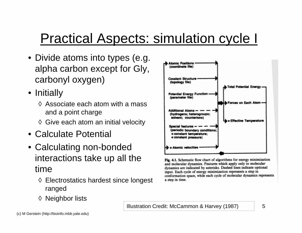
Practical Aspects: simulation cycle I• Divide atoms into types (e.g.

alpha carbon except for Gly,carbonyl oxygen)

• Initially◊ Associate each atom with a mass

and a point charge

◊ Give each atom an initial velocity

• Calculate Potential• Calculating non-bonded

interactions take up all thetime◊ Electrostatics hardest since longest

ranged◊ Neighbor lists

Illustration Credit: McCammon & Harvey (1987)


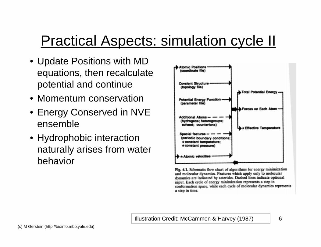
Practical Aspects: simulation cycle II• Update Positions with MD

equations, then recalculatepotential and continue

• Momentum conservation• Energy Conserved in NVE

ensemble• Hydrophobic interaction

naturally arises from waterbehavior

Illustration Credit: McCammon & Harvey (1987)


Major Protein Simulation Packages

• AMBER◊ http://www.amber.ucsf.edu/amber/amber.html

◊ http://www.amber.ucsf.edu/amber/tutorial/index.html

• CHARMM/XPLOR◊ http://yuri.harvard.edu/charmm/charmm.html

◊ http://atb.csb.yale.edu/xplor◊ http://uracil.cmc.uab.edu/Tutorials/default.html

• ENCAD• GROMOS

◊ http://rugmd0.chem.rug.nl/md.html

◊ “Advanced Crash Course on Electrostatics in Simulations” (!)(http://rugmd0.chem.rug.nl/~berends/course.html)


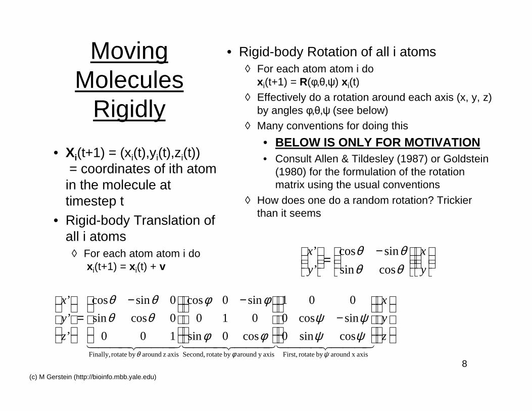
MovingMolecules

Rigidly

• Rigid-body Rotation of all i atoms◊ For each atom atom i do

xi(t+1) = R(φ,θ,ψ) xi(t)◊ Effectively do a rotation around each axis (x, y, z)

by angles φ,θ,ψ (see below)◊ Many conventions for doing this

• BELOW IS ONLY FOR MOTIVATION• Consult Allen & Tildesley (1987) or Goldstein

(1980) for the formulation of the rotationmatrix using the usual conventions

◊ How does one do a random rotation? Trickierthan it seems

−=

y

x

y

x

θθθθ

cossin

sincos

’

’

−

−

−=

z

y

x

z

y

x

444 3444 21444 3444 21444 3444 21axis x around by rotate First,axisy around by rotate Second,axis z around by rotate Finally,

cossin0

sincos0

001

cos0sin

010

sin0cos

100

0cossin

0sincos

’

’

’

ψφθ

ψψψψ

φφ

φφθθθθ

• Xi(t+1) = (xi(t),yi(t),zi(t)) = coordinates of ith atomin the molecule attimestep t

• Rigid-body Translation ofall i atoms

◊ For each atom atom i do xi(t+1) = xi(t) + v


Simulation, Part II:Analysis: What can be

Calculated from Simulation?


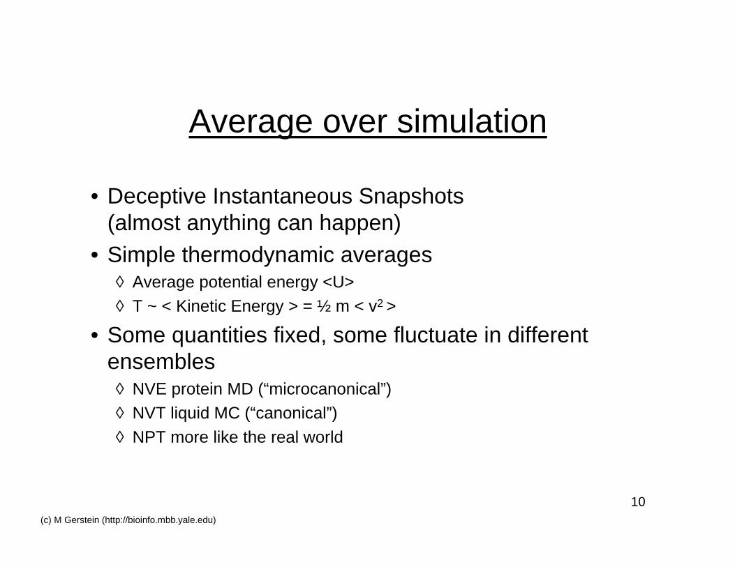
Average over simulation

• Deceptive Instantaneous Snapshots(almost anything can happen)

• Simple thermodynamic averages◊ Average potential energy <U>

◊ T ~ < Kinetic Energy > = ½ m < v2 >

• Some quantities fixed, some fluctuate in differentensembles◊ NVE protein MD (“microcanonical”)◊ NVT liquid MC (“canonical”)

◊ NPT more like the real world


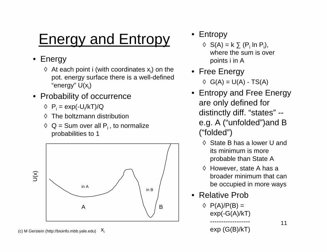
Energy and Entropy• Energy

◊ At each point i (with coordinates xi) on thepot. energy surface there is a well-defined“energy” U(xi)

• Probability of occurrence◊ Pi = exp(-Ui/kT)/Q

◊ The boltzmann distribution◊ Q = Sum over all Pi , to normalize

probabilities to 1

xi

A B

U(x

)

in Ain B

• Entropy◊ S(A) = k ∑ (Pi ln Pi),

where the sum is overpoints i in A

• Free Energy◊ G(A) = U(A) - TS(A)

• Entropy and Free Energyare only defined fordistinctly diff. “states” --e.g. A (“unfolded”)and B(“folded”)

◊ State B has a lower U andits minimum is moreprobable than State A

◊ However, state A has abroader minimum that canbe occupied in more ways

• Relative Prob◊ P(A)/P(B) =

exp(-G(A)/kT)------------------exp (G(B)/kT)


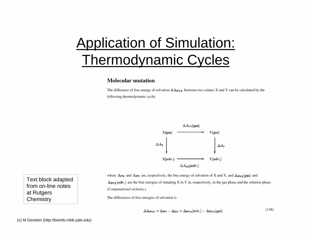
Application of Simulation:Thermodynamic Cycles

Text block adaptedfrom on-line notesat RutgersChemistry


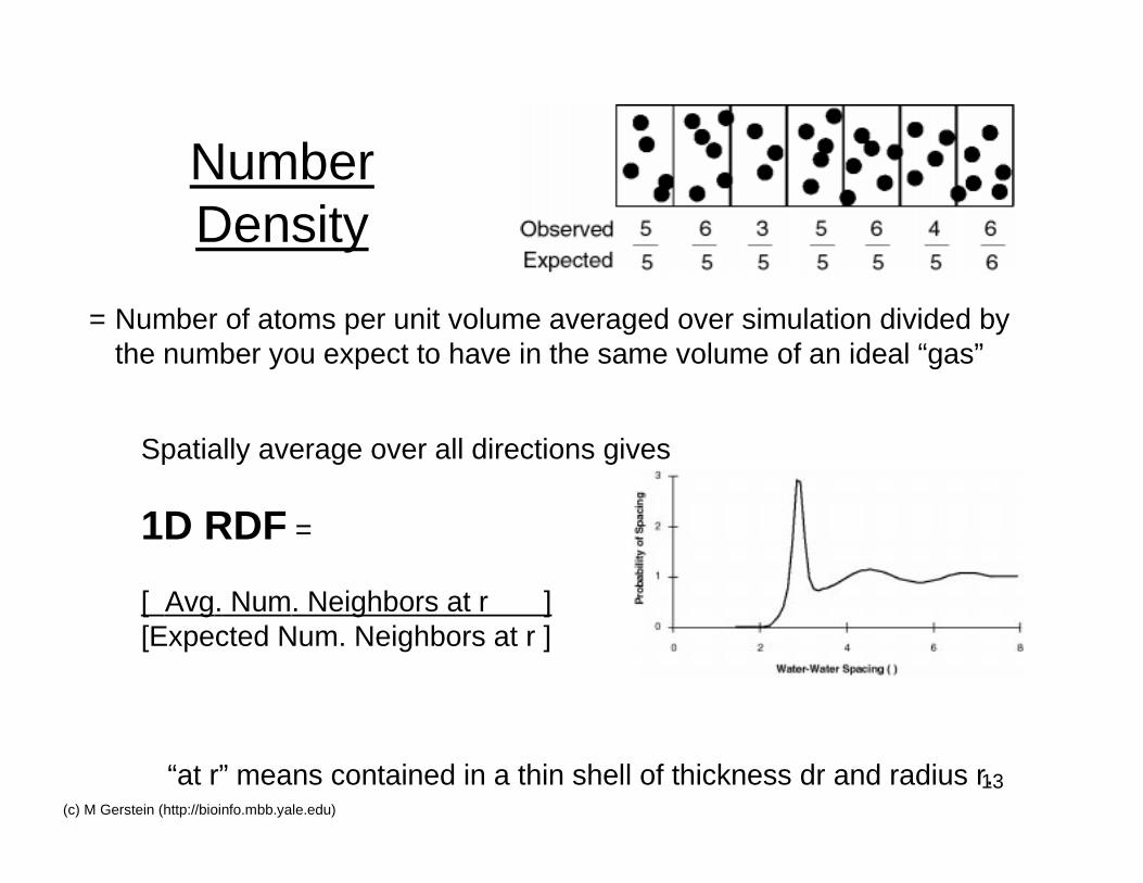
NumberDensity

= Number of atoms per unit volume averaged over simulation divided bythe number you expect to have in the same volume of an ideal “gas”

Spatially average over all directions gives

1D RDF =

[ Avg. Num. Neighbors at r ][Expected Num. Neighbors at r ]

“at r” means contained in a thin shell of thickness dr and radius r.


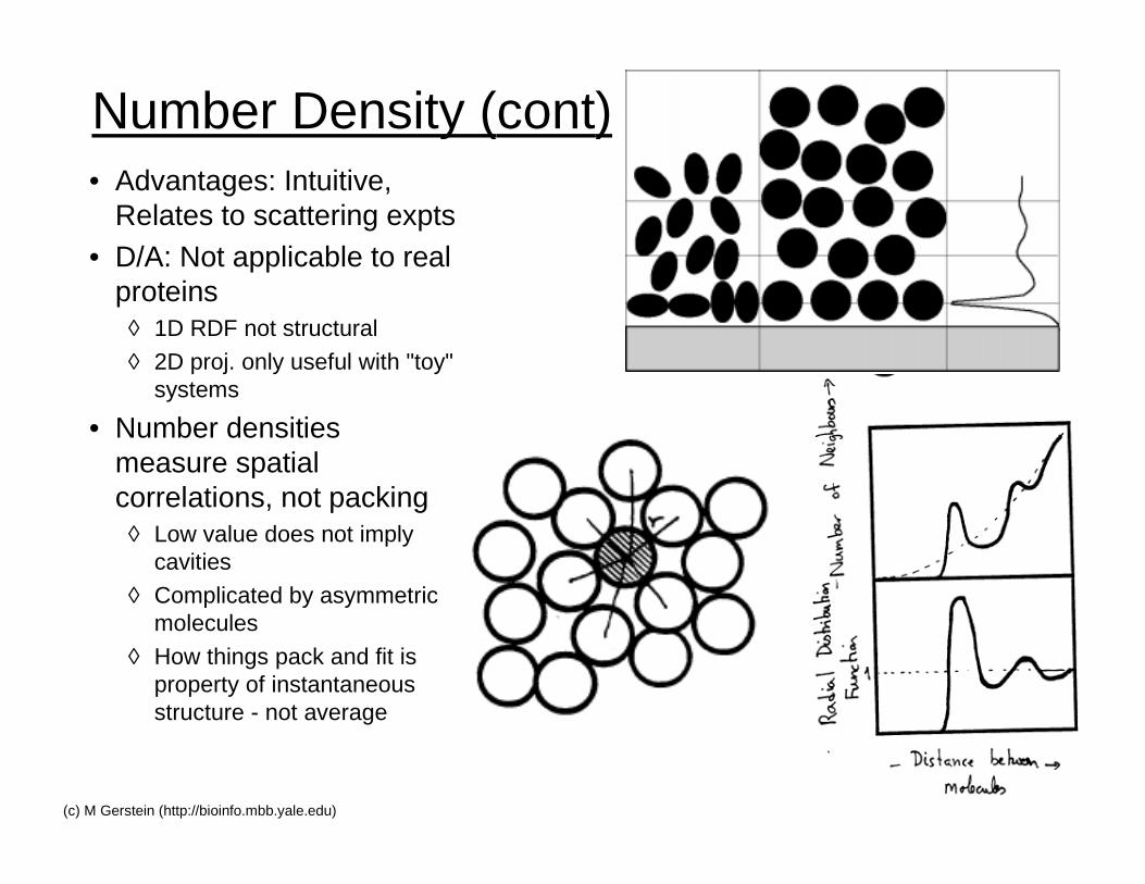
Number Density (cont)• Advantages: Intuitive,

Relates to scattering expts• D/A: Not applicable to real

proteins◊ 1D RDF not structural

◊ 2D proj. only useful with "toy"systems

• Number densitiesmeasure spatialcorrelations, not packing

◊ Low value does not implycavities

◊ Complicated by asymmetricmolecules

◊ How things pack and fit isproperty of instantaneousstructure - not average


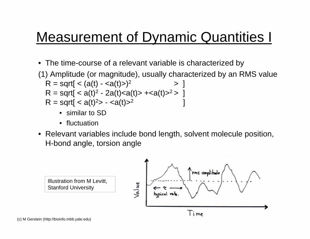
Measurement of Dynamic Quantities I

• The time-course of a relevant variable is characterized by(1) Amplitude (or magnitude), usually characterized by an RMS value

R = sqrt[ < (a(t) - <a(t)>)2 > ]R = sqrt[ < a(t)2 - 2a(t)<a(t)> +<a(t)>2 > ]R = sqrt[ < a(t)2> - <a(t)>2 ]

• similar to SD

• fluctuation

• Relevant variables include bond length, solvent molecule position,H-bond angle, torsion angle

Illustration from M Levitt,Stanford University


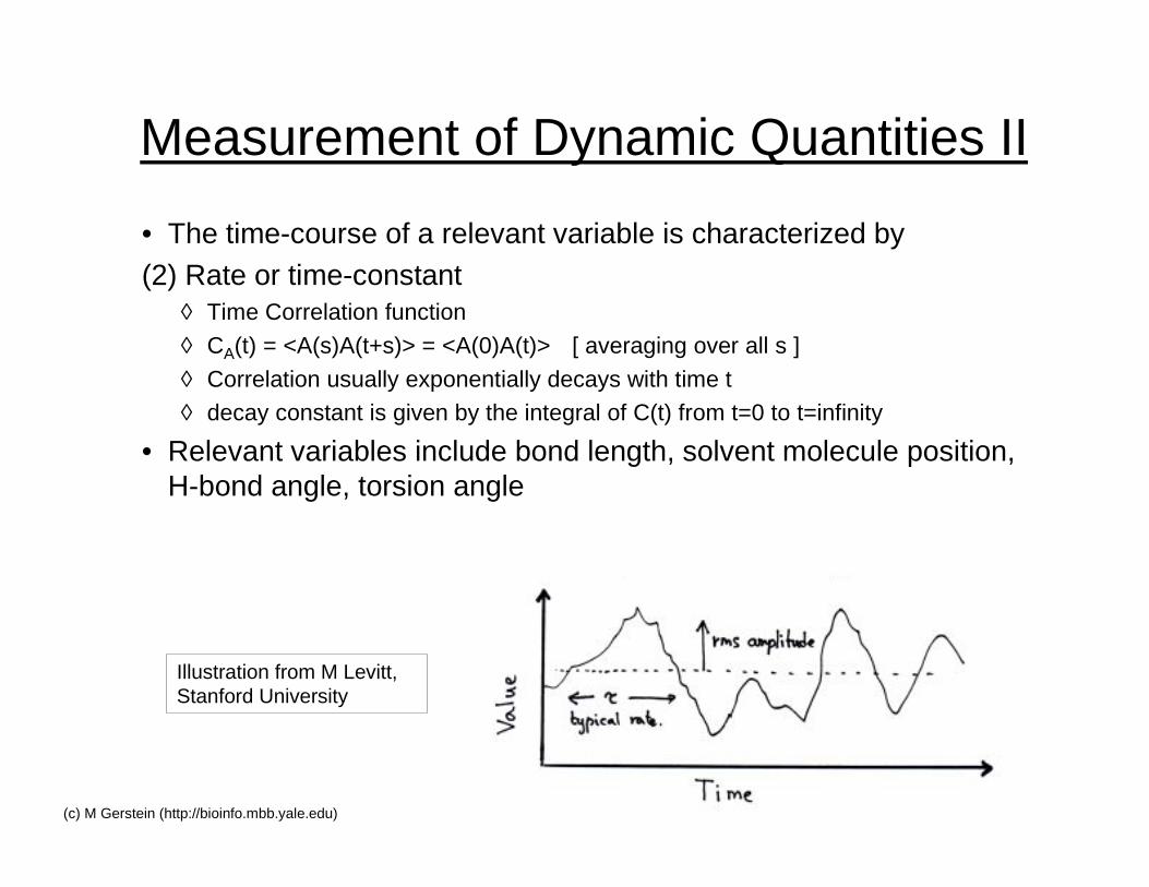
Measurement of Dynamic Quantities II

• The time-course of a relevant variable is characterized by(2) Rate or time-constant

◊ Time Correlation function

◊ CA(t) = <A(s)A(t+s)> = <A(0)A(t)> [ averaging over all s ]

◊ Correlation usually exponentially decays with time t◊ decay constant is given by the integral of C(t) from t=0 to t=infinity

• Relevant variables include bond length, solvent molecule position,H-bond angle, torsion angle



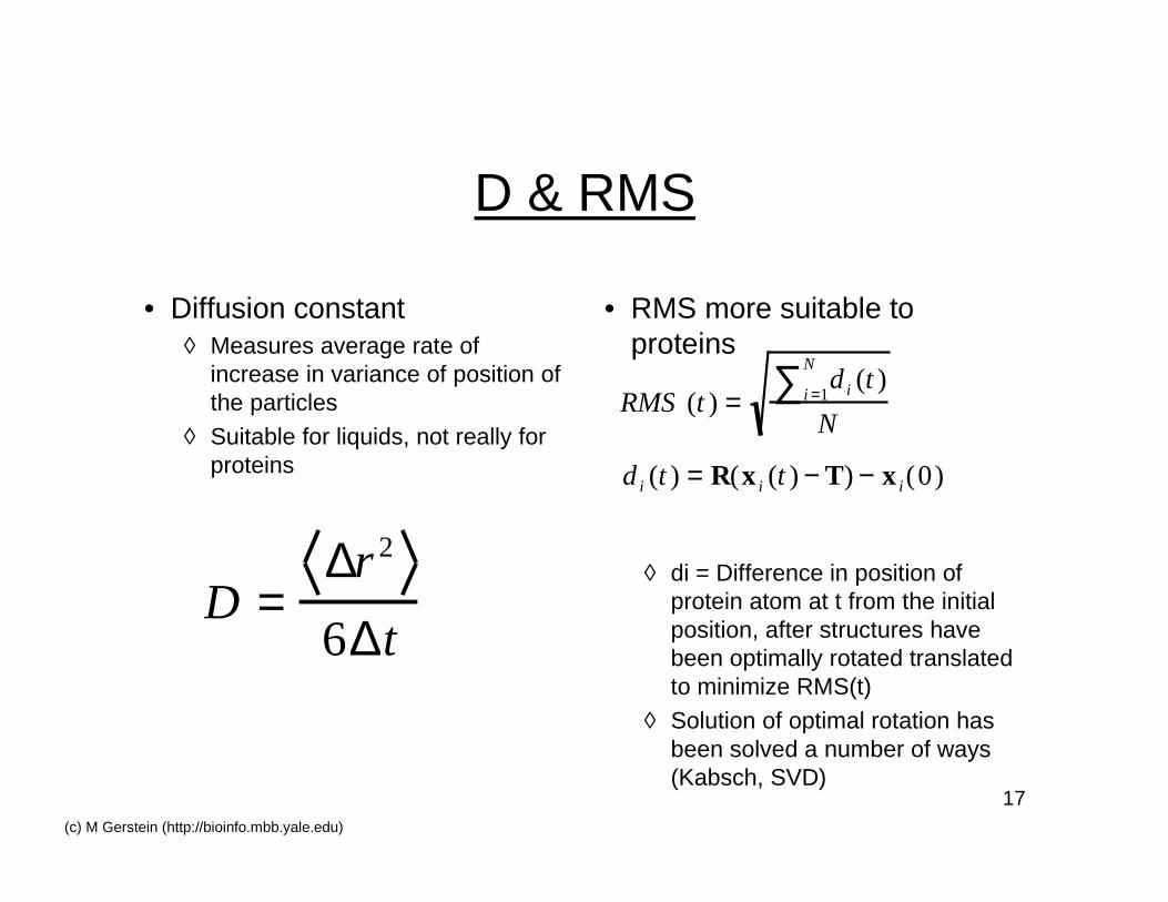
D & RMS

• Diffusion constant◊ Measures average rate of

increase in variance of position ofthe particles

◊ Suitable for liquids, not really forproteins

D =∆r 2

6∆t

RMS (t ) =di (t )

i =1

N∑N

di (t ) = R(x i (t ) − T) − x i(0)

• RMS more suitable toproteins

◊ di = Difference in position ofprotein atom at t from the initialposition, after structures havebeen optimally rotated translatedto minimize RMS(t)

◊ Solution of optimal rotation hasbeen solved a number of ways(Kabsch, SVD)


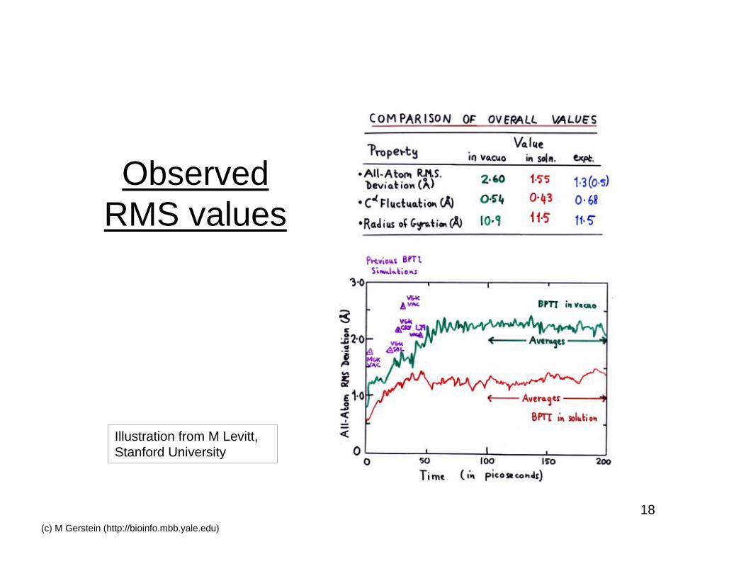
ObservedRMS values



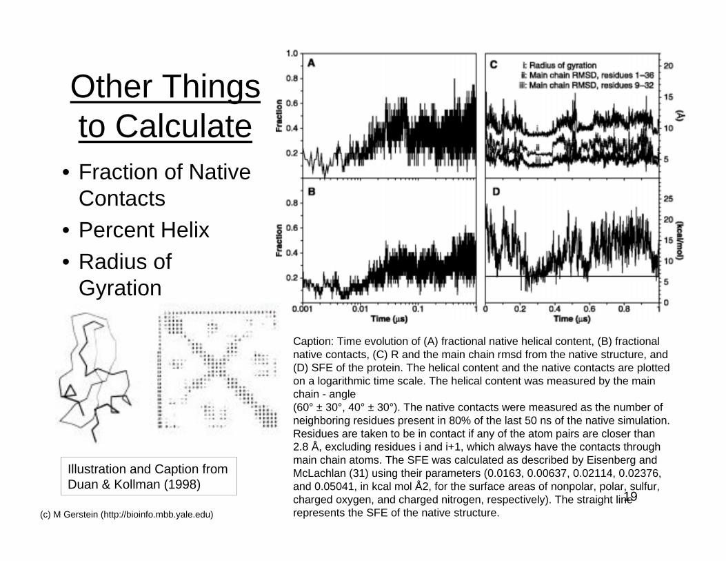
Other Thingsto Calculate

• Fraction of NativeContacts

• Percent Helix• Radius of

Gyration

Illustration and Caption fromDuan & Kollman (1998)

Caption: Time evolution of (A) fractional native helical content, (B) fractionalnative contacts, (C) R and the main chain rmsd from the native structure, and(D) SFE of the protein. The helical content and the native contacts are plottedon a logarithmic time scale. The helical content was measured by the mainchain - angle(60° ± 30°, 40° ± 30°). The native contacts were measured as the number ofneighboring residues present in 80% of the last 50 ns of the native simulation.Residues are taken to be in contact if any of the atom pairs are closer than2.8 Å, excluding residues i and i+1, which always have the contacts throughmain chain atoms. The SFE was calculated as described by Eisenberg andMcLachlan (31) using their parameters (0.0163, 0.00637, 0.02114, 0.02376,and 0.05041, in kcal mol Å2, for the surface areas of nonpolar, polar, sulfur,charged oxygen, and charged nitrogen, respectively). The straight linerepresents the SFE of the native structure.


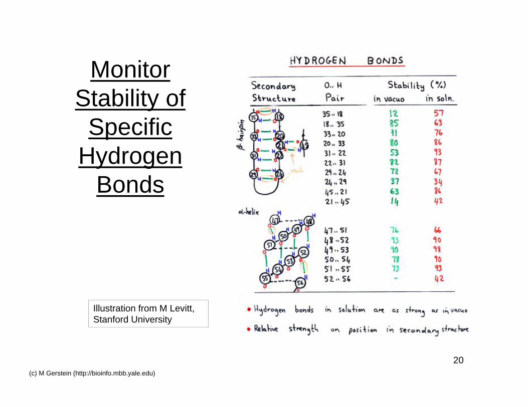
MonitorStability of

SpecificHydrogen

Bonds



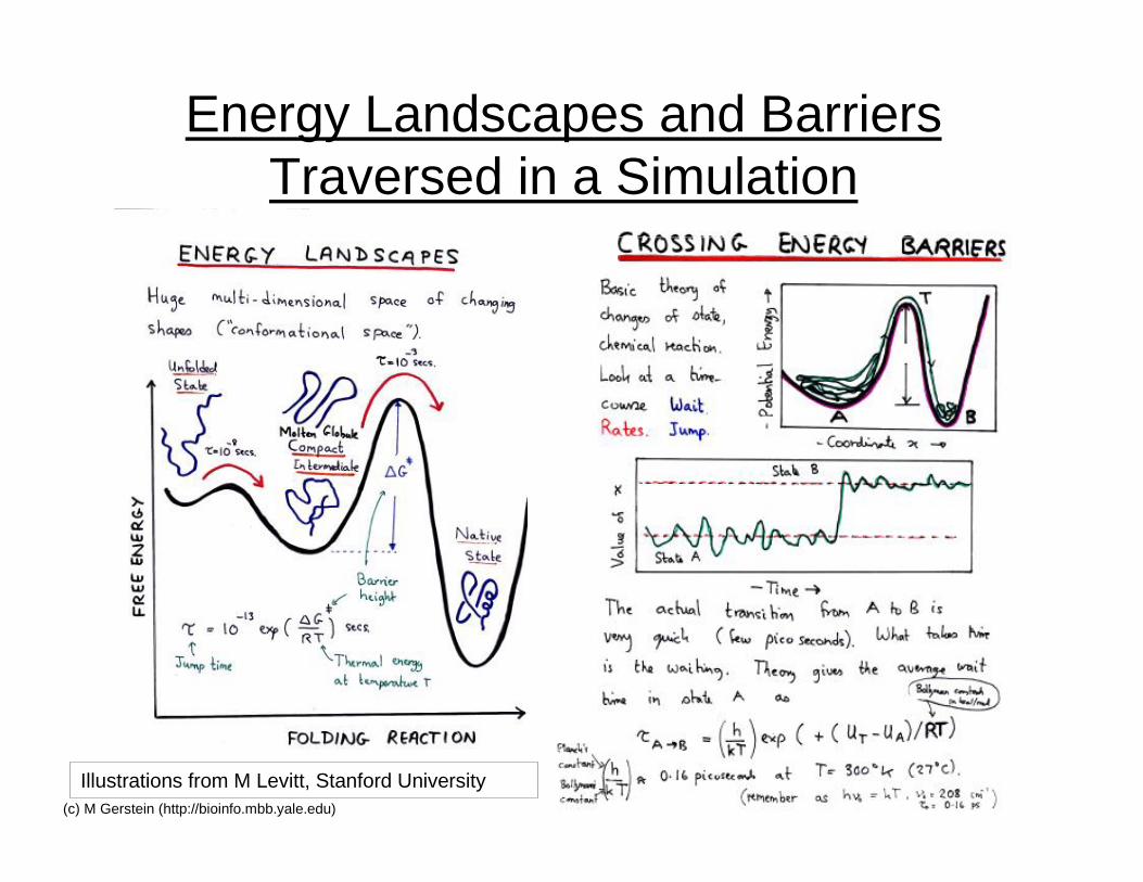
Energy Landscapes and BarriersTraversed in a Simulation

Illustrations from M Levitt, Stanford University


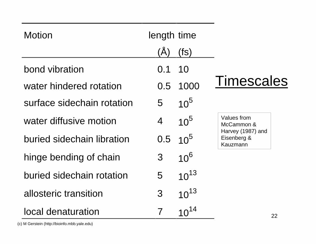
Timescales

Motion length time

(Å) (fs)

bond vibration 0.1 10

water hindered rotation 0.5 1000

surface sidechain rotation 5 105

water diffusive motion 4 105

buried sidechain libration 0.5 105

hinge bending of chain 3 106

buried sidechain rotation 5 1013

allosteric transition 3 1013

local denaturation 7 1014

Values fromMcCammon &Harvey (1987) andEisenberg &Kauzmann


Electrostatics Revisited:the Poisson-Boltzmann Equation


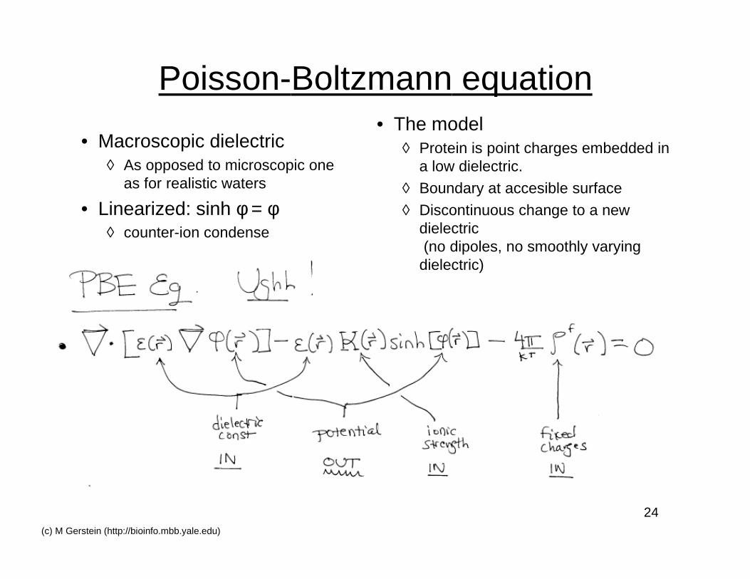
Poisson-Boltzmann equation

• Macroscopic dielectric◊ As opposed to microscopic one

as for realistic waters

• Linearized: sinh φ = φ◊ counter-ion condense

• The model◊ Protein is point charges embedded in

a low dielectric.

◊ Boundary at accesible surface

◊ Discontinuous change to a newdielectric (no dipoles, no smoothly varyingdielectric)


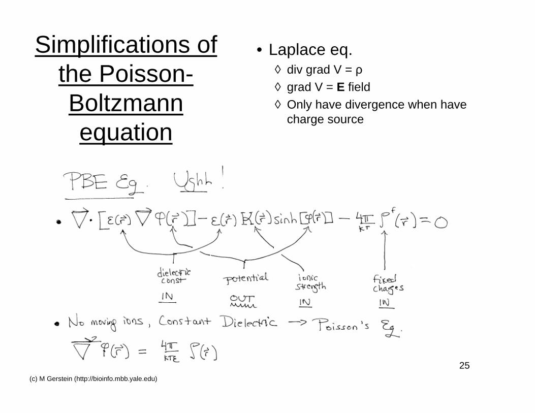
Simplifications ofthe Poisson-Boltzmannequation

• Laplace eq.◊ div grad V = ρ◊ grad V = E field◊ Only have divergence when have

charge source


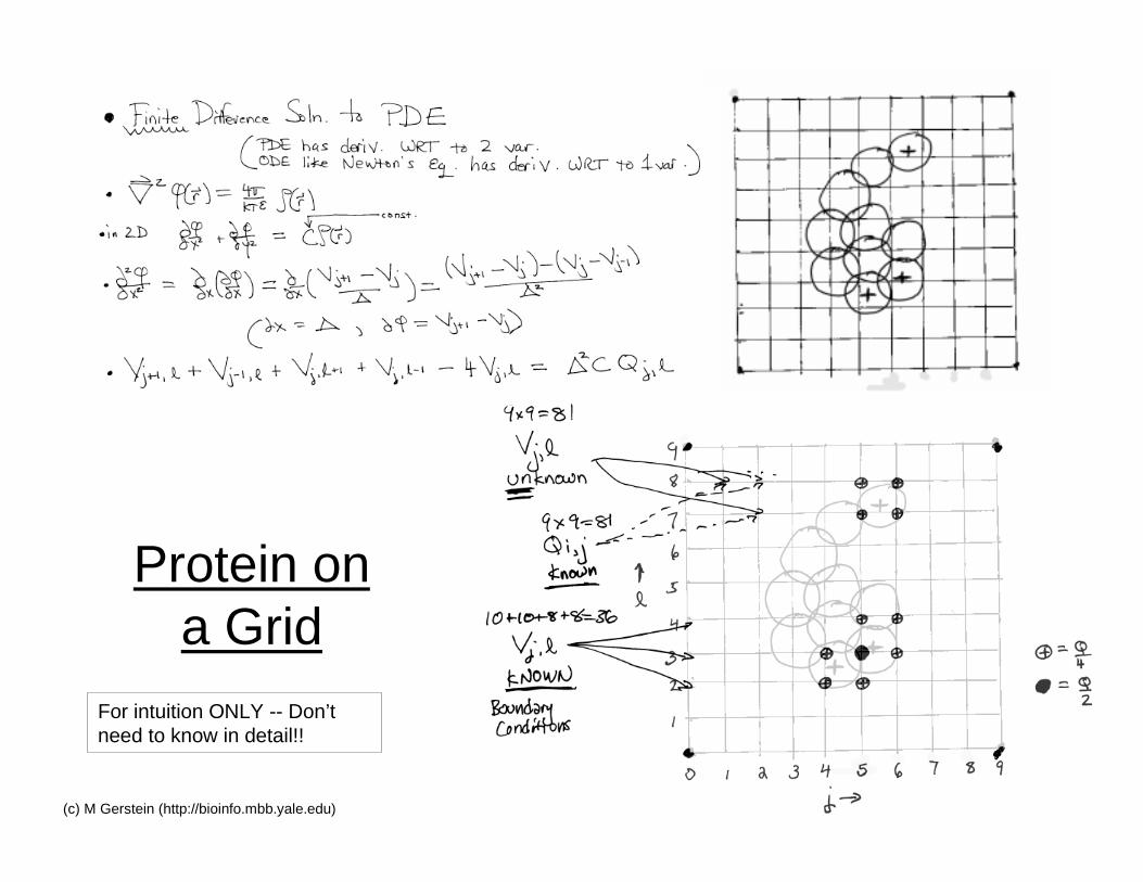
Protein ona Grid

For intuition ONLY -- Don’tneed to know in detail!!


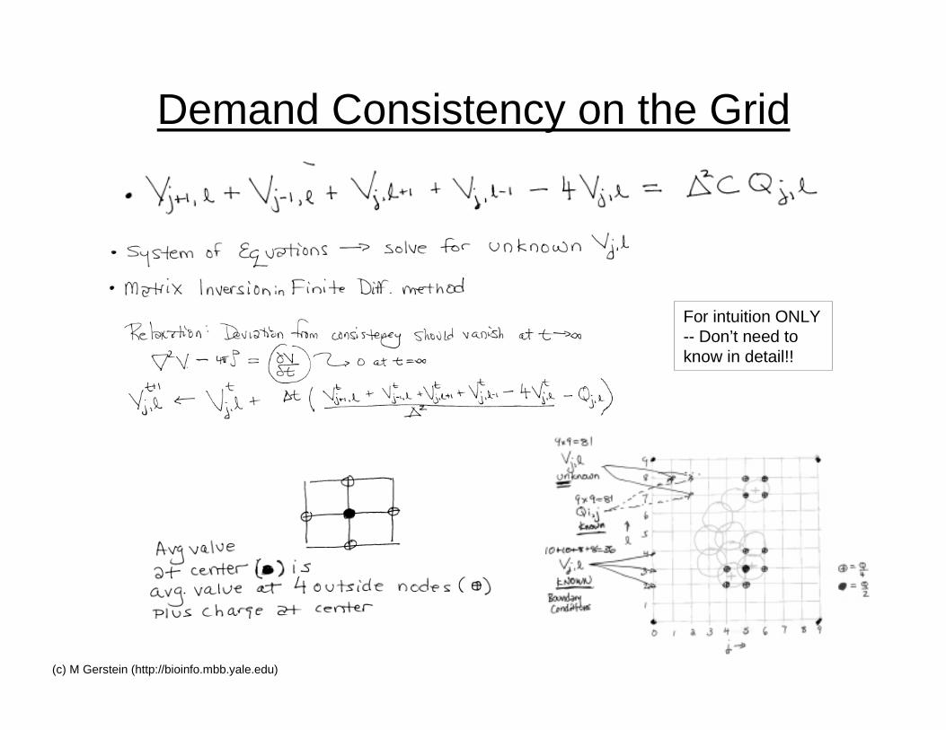
Demand Consistency on the Grid

For intuition ONLY-- Don’t need toknow in detail!!


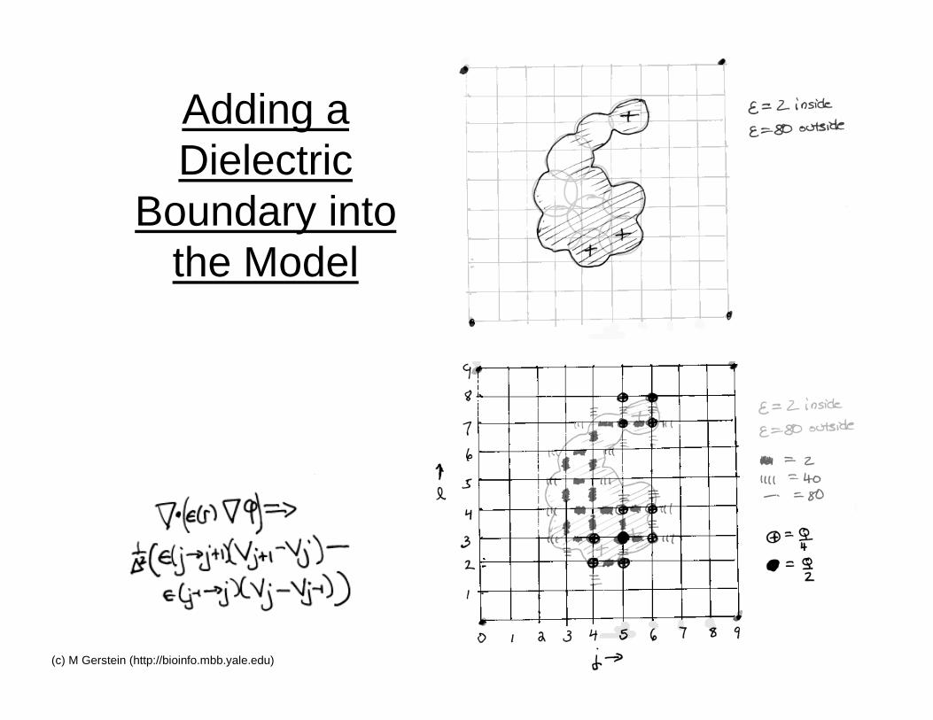
Adding aDielectric

Boundary intothe Model


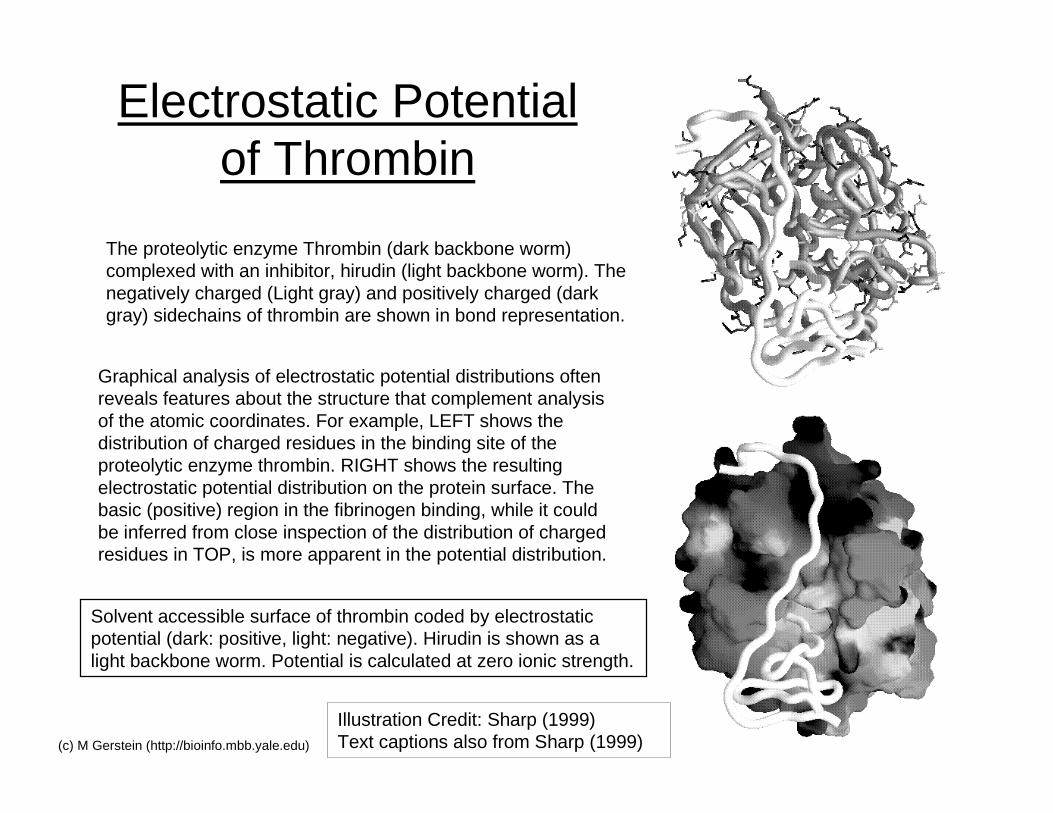
Electrostatic Potentialof Thrombin

The proteolytic enzyme Thrombin (dark backbone worm)complexed with an inhibitor, hirudin (light backbone worm). Thenegatively charged (Light gray) and positively charged (darkgray) sidechains of thrombin are shown in bond representation.

Solvent accessible surface of thrombin coded by electrostaticpotential (dark: positive, light: negative). Hirudin is shown as alight backbone worm. Potential is calculated at zero ionic strength.

Illustration Credit: Sharp (1999)Text captions also from Sharp (1999)

Graphical analysis of electrostatic potential distributions oftenreveals features about the structure that complement analysisof the atomic coordinates. For example, LEFT shows thedistribution of charged residues in the binding site of theproteolytic enzyme thrombin. RIGHT shows the resultingelectrostatic potential distribution on the protein surface. Thebasic (positive) region in the fibrinogen binding, while it couldbe inferred from close inspection of the distribution of chargedresidues in TOP, is more apparent in the potential distribution.


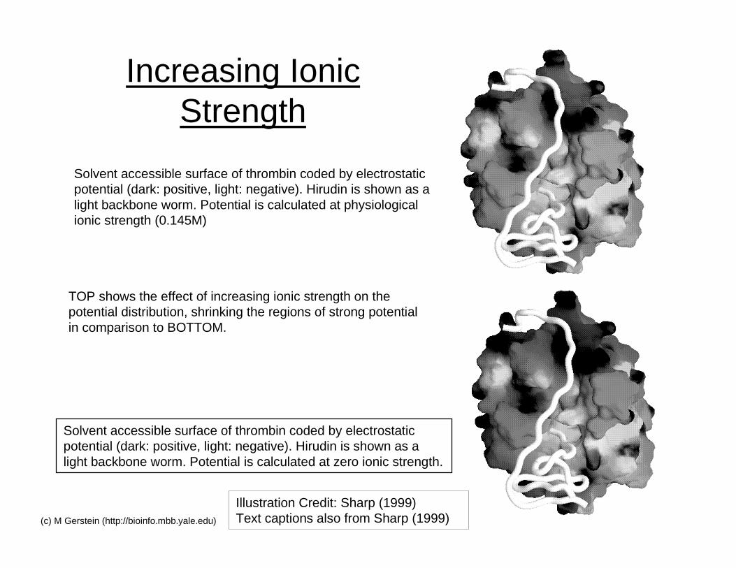
Increasing IonicStrength

Solvent accessible surface of thrombin coded by electrostaticpotential (dark: positive, light: negative). Hirudin is shown as alight backbone worm. Potential is calculated at physiologicalionic strength (0.145M)



TOP shows the effect of increasing ionic strength on thepotential distribution, shrinking the regions of strong potentialin comparison to BOTTOM.


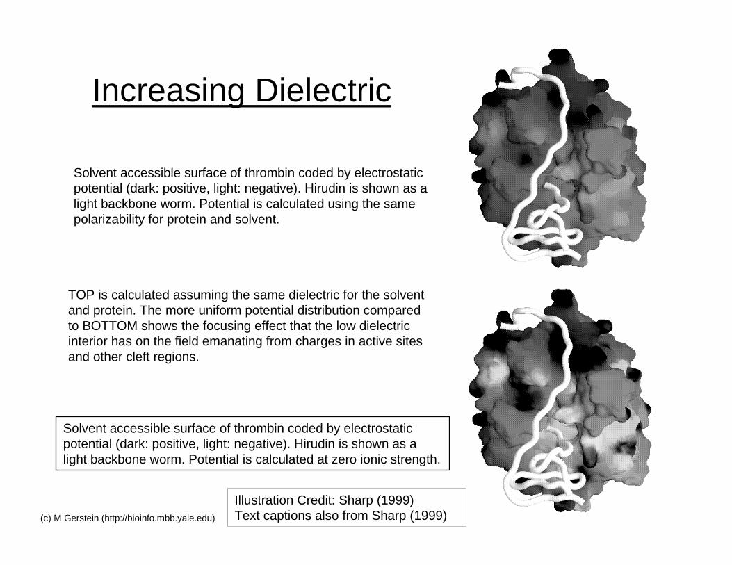
Increasing Dielectric

Solvent accessible surface of thrombin coded by electrostaticpotential (dark: positive, light: negative). Hirudin is shown as alight backbone worm. Potential is calculated using the samepolarizability for protein and solvent.



TOP is calculated assuming the same dielectric for the solventand protein. The more uniform potential distribution comparedto BOTTOM shows the focusing effect that the low dielectricinterior has on the field emanating from charges in active sitesand other cleft regions.


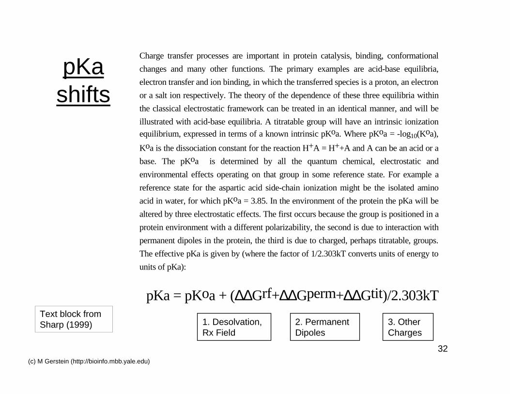
pKashifts

Charge transfer processes are important in protein catalysis, binding, conformational

changes and many other functions. The primary examples are acid-base equilibria,

electron transfer and ion binding, in which the transferred species is a proton, an electron

or a salt ion respectively. The theory of the dependence of these three equilibria within

the classical electrostatic framework can be treated in an identical manner, and will be

illustrated with acid-base equilibria. A titratable group will have an intrinsic ionizationequilibrium, expressed in terms of a known intrinsic pKoa. Where pKoa = -log10(Koa),

Koa is the dissociation constant for the reaction H+A = H++A and A can be an acid or a

base. The pKoa is determined by all the quantum chemical, electrostatic and

environmental effects operating on that group in some reference state. For example a

reference state for the aspartic acid side-chain ionization might be the isolated amino

acid in water, for which pKoa = 3.85. In the environment of the protein the pKa will be

altered by three electrostatic effects. The first occurs because the group is positioned in a

protein environment with a different polarizability, the second is due to interaction with

permanent dipoles in the protein, the third is due to charged, perhaps titratable, groups.

The effective pKa is given by (where the factor of 1/2.303kT converts units of energy to

units of pKa):

pKa = pKoa + (∆∆Grf+∆∆Gperm+∆∆Gtit)/2.303kTText block fromSharp (1999) 1. Desolvation,

Rx Field2. PermanentDipoles

3. OtherCharges


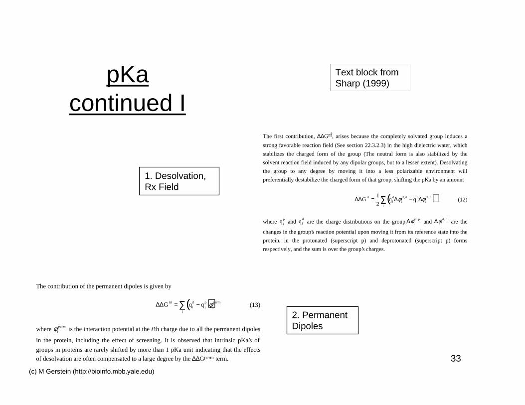
pKacontinued I

The first contribution, ∆∆Grf, arises because the completely solvated group induces a

strong favorable reaction field (See section 22.3.2.3) in the high dielectric water, which

stabilizes the charged form of the group (The neutral form is also stabilized by the

solvent reaction field induced by any dipolar groups, but to a lesser extent). Desolvating

the group to any degree by moving it into a less polarizable environment will

preferentially destabilize the charged form of that group, shifting the pKa by an amount

∆∆G rf =1

2qi

d∆φi

rf,d − qi

p∆φi

rf ,p( )i

∑ (12)

where qi

p and qi

d are the charge distributions on the group,∆φ

i

rf, p and ∆φ

i

rf, d are the

changes in the group’s reaction potential upon moving it from its reference state into the

protein, in the protonated (superscript p) and deprotonated (superscript p) forms

respectively, and the sum is over the group’s charges.

The contribution of the permanent dipoles is given by

∆∆G tit = qid − q

i

p( )i

∑ φi

perm (13)

where φ i

perm is the interaction potential at the i’th charge due to all the permanent dipoles

in the protein, including the effect of screening. It is observed that intrinsic pKa’s of

groups in proteins are rarely shifted by more than 1 pKa unit indicating that the effects

of desolvation are often compensated to a large degree by the ∆∆Gperm term.

1. Desolvation,Rx Field

2. PermanentDipoles

Text block fromSharp (1999)


pKa continued II

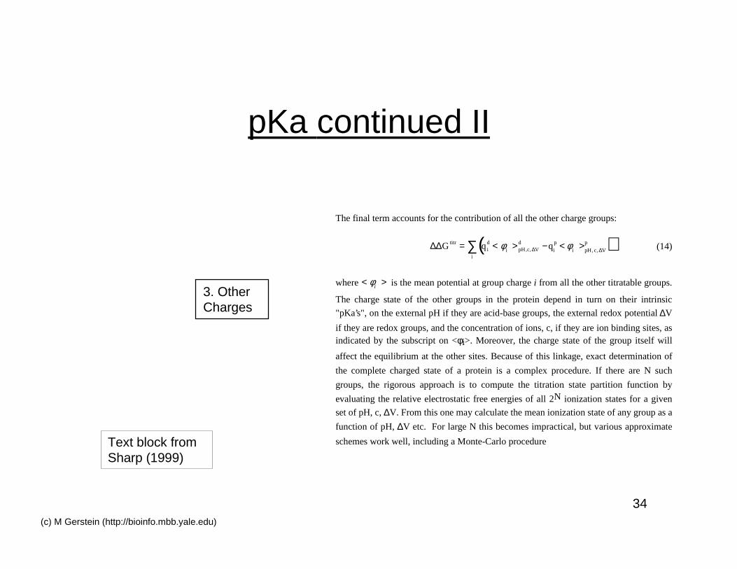
The final term accounts for the contribution of all the other charge groups:

∆∆G titr = qid < φ

i> pH,c, ∆V

d −qi

p < φi

>pH, c, ∆V

p( )i

∑ (14)

where < φi

> is the mean potential at group charge i from all the other titratable groups.

The charge state of the other groups in the protein depend in turn on their intrinsic

"pKa’s", on the external pH if they are acid-base groups, the external redox potential ∆V

if they are redox groups, and the concentration of ions, c, if they are ion binding sites, asindicated by the subscript on <φi>. Moreover, the charge state of the group itself will

affect the equilibrium at the other sites. Because of this linkage, exact determination of

the complete charged state of a protein is a complex procedure. If there are N such

groups, the rigorous approach is to compute the titration state partition function by

evaluating the relative electrostatic free energies of all 2N ionization states for a given

set of pH, c, ∆V. From this one may calculate the mean ionization state of any group as a

function of pH, ∆V etc. For large N this becomes impractical, but various approximate

schemes work well, including a Monte-Carlo procedure

3. OtherCharges

Text block fromSharp (1999)


Water Simulationand Hydrophobicity


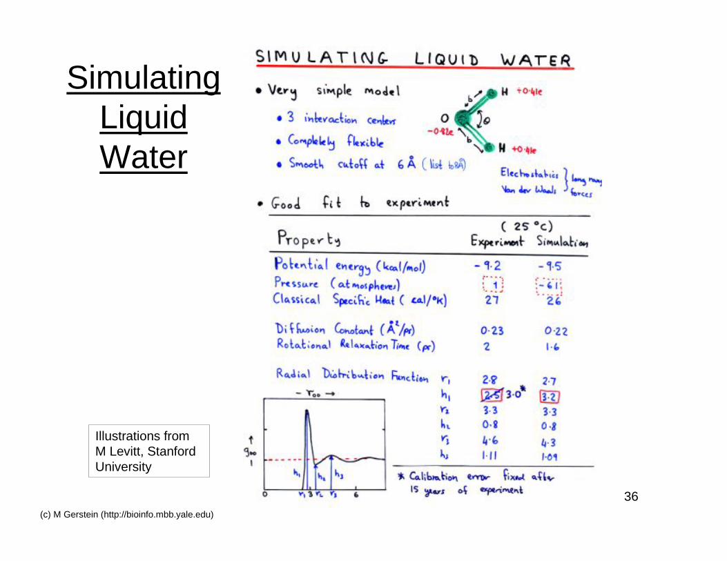
SimulatingLiquidWater

Illustrations fromM Levitt, StanfordUniversity


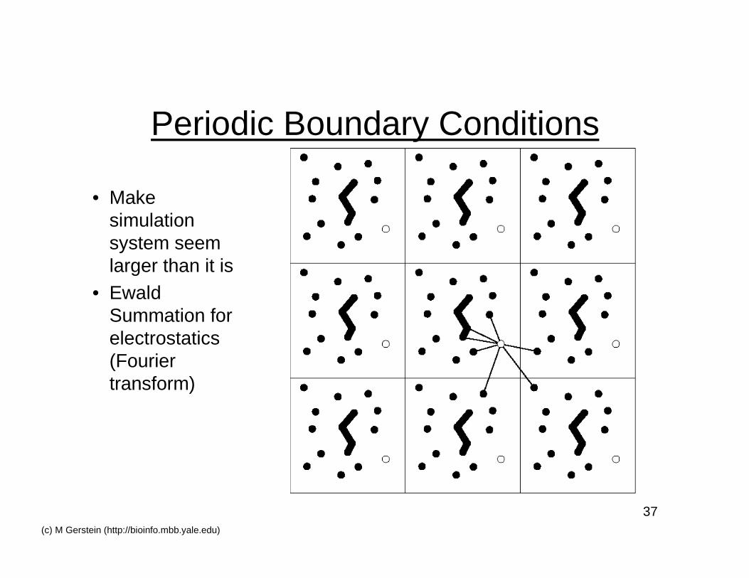
Periodic Boundary Conditions

• Makesimulationsystem seemlarger than it is

• EwaldSummation forelectrostatics(Fouriertransform)


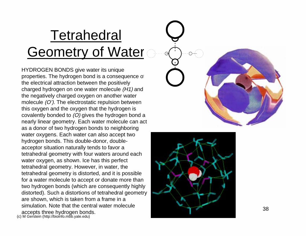
TetrahedralGeometry of Water

HYDROGEN BONDS give water its uniqueproperties. The hydrogen bond is a consequence ofthe electrical attraction between the positivelycharged hydrogen on one water molecule (H1) andthe negatively charged oxygen on another watermolecule (O’). The electrostatic repulsion betweenthis oxygen and the oxygen that the hydrogen iscovalently bonded to (O) gives the hydrogen bond anearly linear geometry. Each water molecule can actas a donor of two hydrogen bonds to neighboringwater oxygens. Each water can also accept twohydrogen bonds. This double-donor, double-acceptor situation naturally tends to favor atetrahedral geometry with four waters around eachwater oxygen, as shown. Ice has this perfecttetrahedral geometry. However, in water, thetetrahedral geometry is distorted, and it is possiblefor a water molecule to accept or donate more thantwo hydrogen bonds (which are consequently highlydistorted). Such a distortions of tetrahedral geometryare shown, which is taken from a frame in asimulation. Note that the central water moleculeaccepts three hydrogen bonds.


HydrophobicityArises

Naturallyin Simulation

• Add no hydrophobicEffect◊ This arises naturally

from entropic effectsduring the simulation

M ix in g is a sp o n ta n e o u s p ro c e s s : a s u b s ta n c e w il l n a tu ra l lyd is s o lv e in w a te r u n le ss th e re a re m a n ife s t ly u n fa v o ra b le in te ra c tio n sb e tw e e n i t a n d w a te r . S c ie n tis ts u su a lly d is c u s s th e fa v o ra b le n e s s o fp a r t ic u la r in te ra c tio n s in te rm s o f th e e n e rg y a s so c ia te d w ith th ein te rm o le c u la r fo rc e s . A lm o s t a lw a y s th e re a re a t le a s t s o m e e n e rg e tic a l lyfa v o ra b le d is p e r s io n in te ra c tio n s b e tw e e n th e s o lu te a n d th e w a te r .H o w e v e r , th e m o re s a l ie n t is s u e is h o w th e in te ra c tio n b e tw e e n a s o lu tea n d a w a te r m o le c u le c o m p a r e s in s tre n g th to th e in te ra c tio n b e tw e e n tw ow a te r m o le c u le s o r b e tw e e n tw o s o lu te m o le c u le s . F o r in s ta n c e , a p o la rm o le c u le s u c h a s g lu c o s e is a b le to m a k e c o m p a ra b le h y d ro g e n b o n d s tow a te r a s w a te r m o le c u le s c a n m a k e w ith e a c h o th e r . T h u s , th e re a re n ou n fa v o ra b le in te ra c tio n s p re v e n tin g i t f ro m d is s o lv in g a n d i t is v e rys o lu b le .

In c o n tra s t , w a te r m o le c u le s a re n o t a b le to h y d ro g e n b o n d tom e th a n e , a n in so lu b le , n o n -p o la r so lu te . T h e y w o u ld r a th e r in te ra c t w ithe a c h o th e r . T h e m e th a n e m o le c u le s , m o re o v e r , c a n f a v o ra b ly in te ra c tw ith e a c h o th e r th ro u g h a t tra c t iv e d isp e rs io n fo rc e s . O n e c a n s e e h o w th iss i tu a tio n le a d s to m e th a n e m o le c u le s try in g to m in im iz e th e ir r e la tiv e lyu n fa v o ra b le in te ra c tio n s w ith w a te r m o le c u le s . A n o b v io u s w a y th e y c a nd o th is is b y c lu m p in g to g e th e r , a g g re g a tin g , a n d c o m in g o u t s o lu tio n .S u c h a g g re g a tio n o f n o n -p o la r s o lu te s in w a te r is o f te n c a lle d th eh y d r o p h o b ic e f fe c t a n d , a s w e s h a ll , i t is v e ry im p o rta n t inm a c ro m o le c u la r s tru c tu re .

In te rm s o f w a te r s tru c tu re a t ro o m te m p e ra tu re , th e r e la t iv e lyu n fa v o ra b le in te ra c tio n b e tw e e n w a te r a n d m e th a n e in d u c e s e a c h w a te rm o le c u le n e x t to m e th a n e to “ tu rn a w a y ” f ro m i t a n d h y d ro g e n b o n d ton e ig h b o r in g w a te r m o le c u le s . I f o n e o f th e se tu rn e d w a te r m o le c u le sm a n a g e s to k e e p i tse lf c o rre c t ly o r ie n te d o v e r t im e , i t w i l l h a v e w i l l n o th a v e to sa c r i f ic e a n y o f i ts u su a l fo u r to f iv e h y d ro g e n b o n d s . T h is b r in g su p a n in te re s t in g p a ra d o x : F ro m th e s ta n d p o in t o f fa v o ra b le in te ra c t io n s ,o r e n e rg y in m o re fo rm a l te rm in o lo g y , w a te r h a s n o t p a id a n y p r ic e inso lv a t in g th e m e th a n e . C o n se q u e n tly , th e re a p p e a rs to b e n o e n e rg e t icre a so n fo r m e th a n e to b e in so lu b le in w a te r .

T h is p a ra d o x is re so lv e d b y e n tro p y . A c c o rd in g to o n e w a y o fth in k in g , e n tro p y re f le c ts th e n u m b e r o f p o ss ib le s ta te s a m o le c u le c a ne x is t in . T h u s, th e m o re s ta te s a w a te r m o le c u le c a n e x is t in , th e b e tte r i tss i tu a t io n is e n tro p ic a l ly , a n d i f a so lu te “ p in s d o w n ” a w a te r m o le c u le o rre s tr ic ts i ts f re e d o m o f m o tio n , i t is e n tro p ic a l ly u n fa v o ra b le . A l l so lu te sre s tr ic t th e f re e d o m o f m o tio n o f w a te r m o le c u le s to so m e d e g re e , b u tth is is p a r t ic u la r ly tru e fo r a n o n -p o la r so lu te , su c h a s m e th a n e . T h u s ,s in c e tu rn in g a w a y f ro m m e th a n e “ p in s d o w n ” e a c h w a te r m o le c u les l ig h tly , th e p r ic e o f h y d ra t in g th is n o n -p o la r so lu te is p a id in d ire c t ly inte rm s o f e n tro p y a n d n o t d ire c t ly in te rm s o f e n e rg y .

T h e h y d ro p h o b ic e f fe c t is c u rre n t ly re c e iv in g in te n se sc ru tin y f ro ms im u la tio n a n d e x p e r im e n t. T h e p ic tu re th a t is e m e rg in g is so m e w h a tm o re c o m p lic a te d th a n th e s im p l i f ie d a c c o u n t p re se n te d h e re s in c e a th ig h te m p e ra tu re s , h y d ro p h o b ic h y d ra t io n is s t i l l u n fa v o ra b le b u t fo re n e rg e t ic a n d n o t e n tro p ic re a so n s. N e v e r th e le ss , i r re sp e c t iv e o f w h e th e rth e p r ic e is p a id in te rm s o f e n e rg y o r e n tro p y , th e h y d ro p h o b ic e f fe c t isfu n d a m e n ta l ly c a u se d b y th e r e la tiv e ly u n fa v o ra b le in te ra c tio n s b e tw e e nw a te r a n d h y d ro p h o b ic so lu te s .


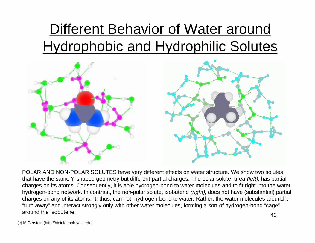
Different Behavior of Water aroundHydrophobic and Hydrophilic Solutes

POLAR AND NON-POLAR SOLUTES have very different effects on water structure. We show two solutesthat have the same Y-shaped geometry but different partial charges. The polar solute, urea (left), has partialcharges on its atoms. Consequently, it is able hydrogen-bond to water molecules and to fit right into the waterhydrogen-bond network. In contrast, the non-polar solute, isobutene (right), does not have (substantial) partialcharges on any of its atoms. It, thus, can not hydrogen-bond to water. Rather, the water molecules around it“turn away” and interact strongly only with other water molecules, forming a sort of hydrogen-bond “cage”around the isobutene.


Consequences of HydrophobicHydration and “Clathrate” Formation

• Hydrophobic hydration is unfavorable (G) but thereason is different at different T◊ entropically (S) unfavorable at low temperatures because of ordering◊ enthalpically (H) unfavorable at high temperatures because of

unsatisified H-bonds

• Volume of mixing is negative• Compressibility• High heat capacity of hydrophobic solvation

◊ Signature of hydrophobic hydration◊ Hydration creates new temperature “labile” structures


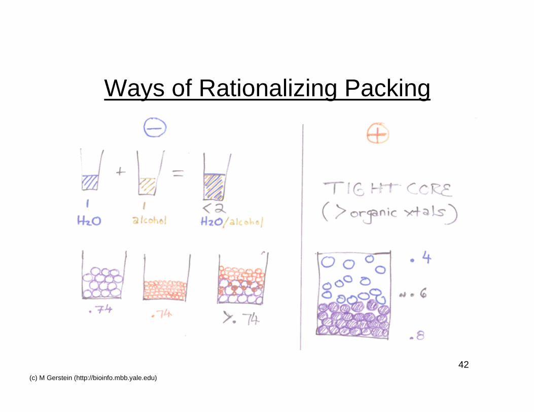
Ways of Rationalizing Packing


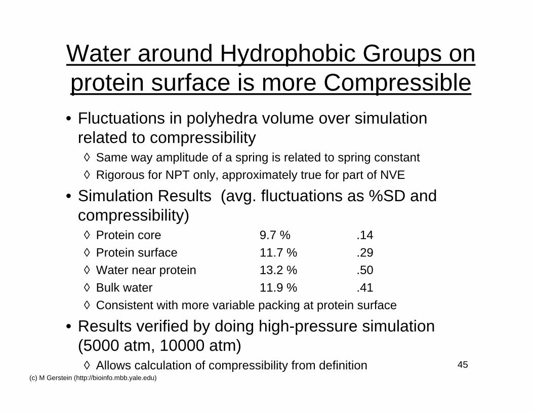
Water around Hydrophobic Groups onprotein surface is more Compressible

• Fluctuations in polyhedra volume over simulationrelated to compressibility◊ Same way amplitude of a spring is related to spring constant◊ Rigorous for NPT only, approximately true for part of NVE

• Simulation Results (avg. fluctuations as %SD andcompressibility)◊ Protein core 9.7 % .14

◊ Protein surface 11.7 % .29◊ Water near protein 13.2 % .50

◊ Bulk water 11.9 % .41

◊ Consistent with more variable packing at protein surface

• Results verified by doing high-pressure simulation(5000 atm, 10000 atm)◊ Allows calculation of compressibility from definition


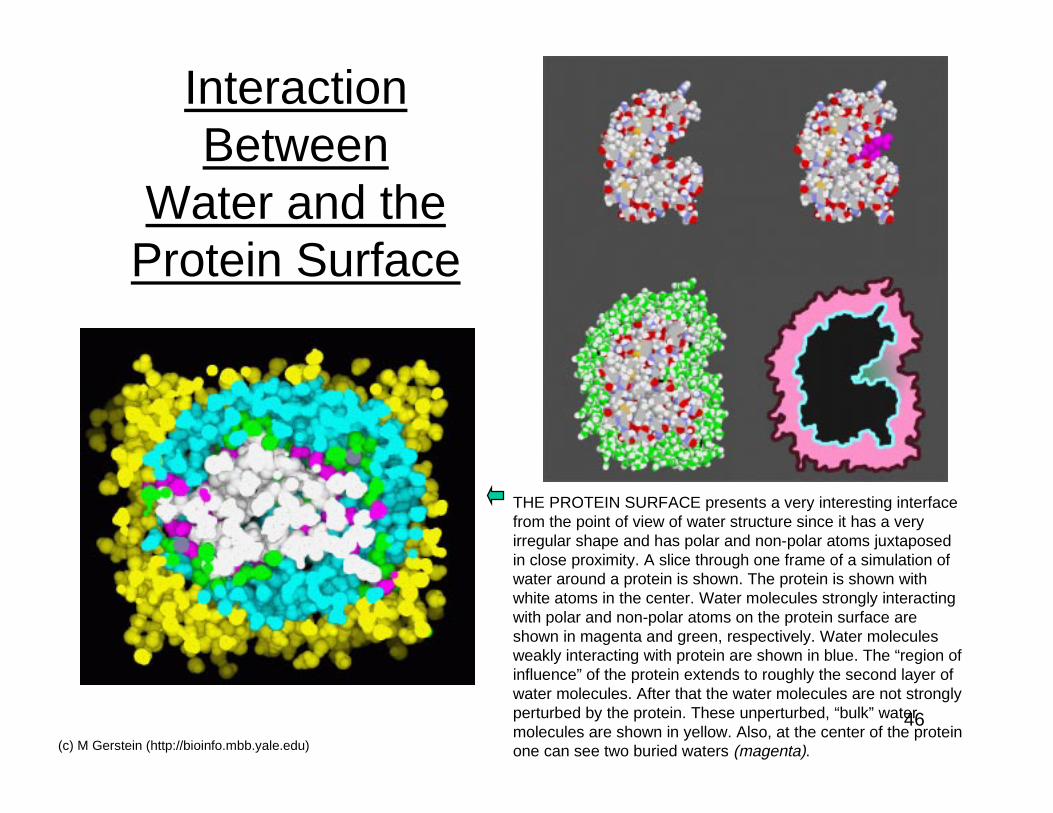
InteractionBetween

Water and theProtein Surface

THE PROTEIN SURFACE presents a very interesting interfacefrom the point of view of water structure since it has a veryirregular shape and has polar and non-polar atoms juxtaposedin close proximity. A slice through one frame of a simulation ofwater around a protein is shown. The protein is shown withwhite atoms in the center. Water molecules strongly interactingwith polar and non-polar atoms on the protein surface areshown in magenta and green, respectively. Water moleculesweakly interacting with protein are shown in blue. The “region ofinfluence” of the protein extends to roughly the second layer ofwater molecules. After that the water molecules are not stronglyperturbed by the protein. These unperturbed, “bulk” watermolecules are shown in yellow. Also, at the center of the proteinone can see two buried waters (magenta).


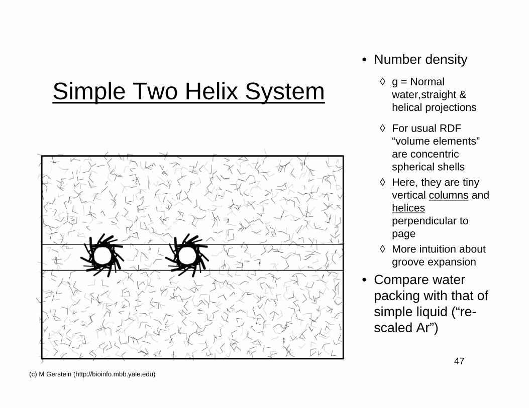
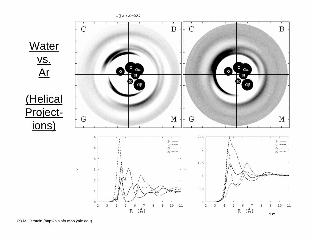
Simple Two Helix System

• Number density

◊ g = Normalwater,straight &helical projections

◊ For usual RDF“volume elements”are concentricspherical shells

◊ Here, they are tinyvertical columns andhelicesperpendicular topage

◊ More intuition aboutgroove expansion

• Compare waterpacking with that ofsimple liquid (“re-scaled Ar”)


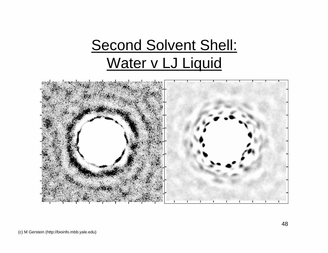
Second Solvent Shell:Water v LJ Liquid


Watervs.Ar

(HelicalProject-

ions)


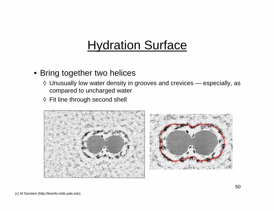
Hydration Surface

• Bring together two helices◊ Unusually low water density in grooves and crevices — especially, as

compared to uncharged water

◊ Fit line through second shell


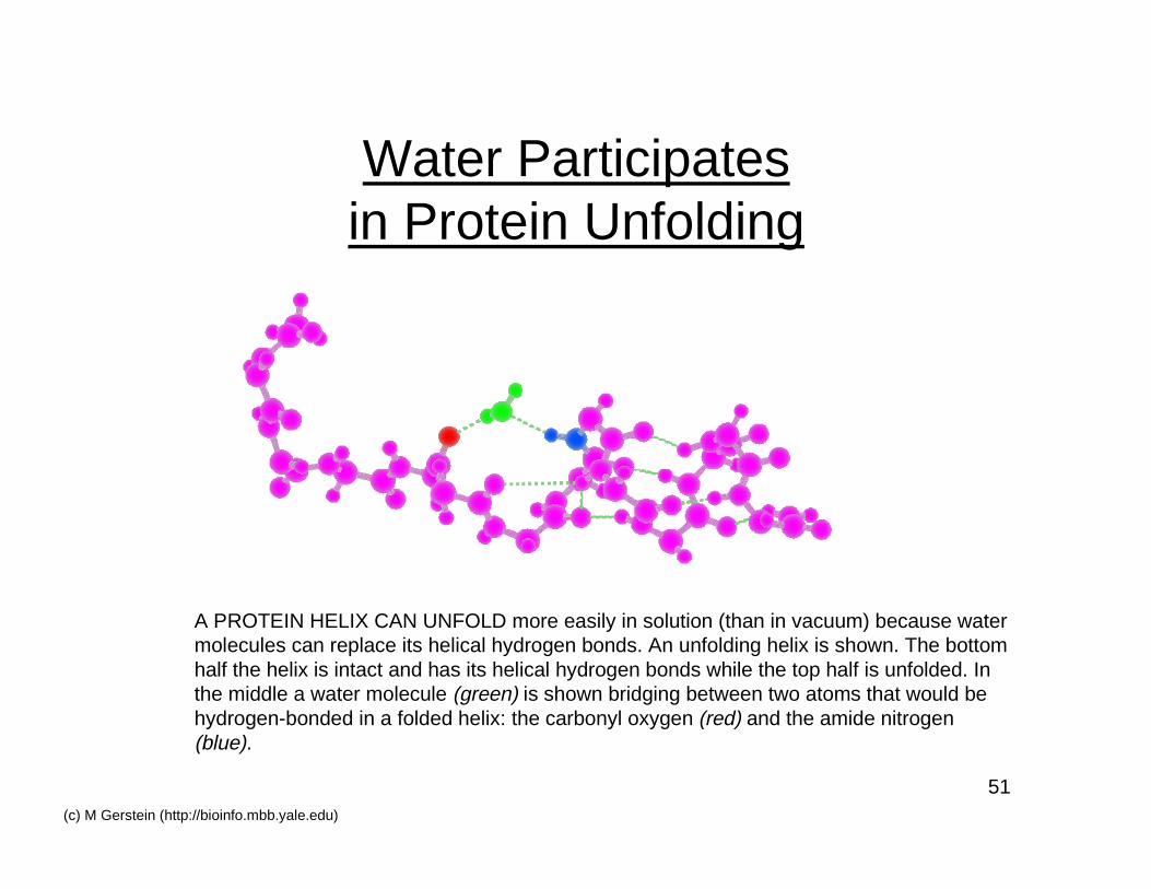
Water Participatesin Protein Unfolding

A PROTEIN HELIX CAN UNFOLD more easily in solution (than in vacuum) because watermolecules can replace its helical hydrogen bonds. An unfolding helix is shown. The bottomhalf the helix is intact and has its helical hydrogen bonds while the top half is unfolded. Inthe middle a water molecule (green) is shown bridging between two atoms that would behydrogen-bonded in a folded helix: the carbonyl oxygen (red) and the amide nitrogen(blue).


Simplified Simulation


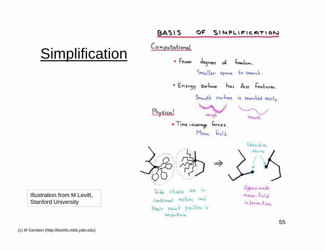
Simplification



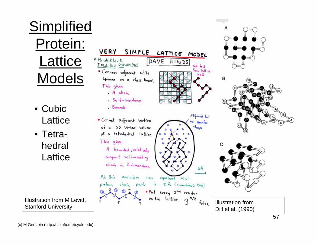
SimplifiedProtein:LatticeModels

• CubicLattice

• Tetra-hedralLattice


Illustration fromDill et al. (1990)


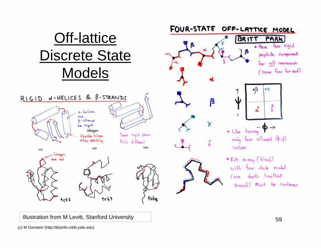
Off-latticeDiscrete State

Models

Illustration from M Levitt, Stanford University


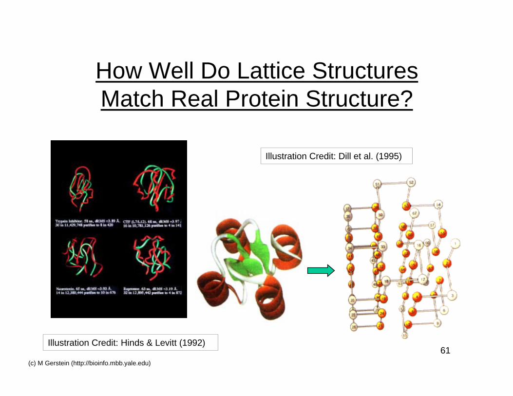
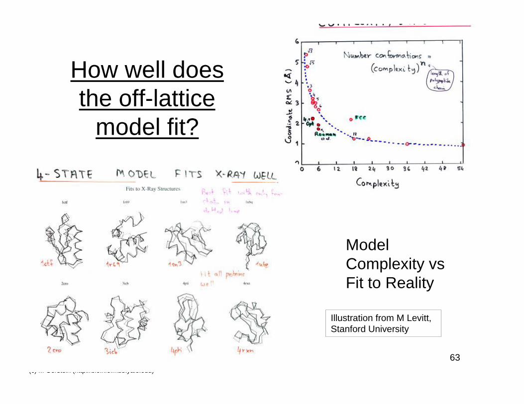
How Well Do Lattice StructuresMatch Real Protein Structure?

Illustration Credit: Dill et al. (1995)

Illustration Credit: Hinds & Levitt (1992)


How well doesthe off-lattice

model fit?

ModelComplexity vsFit to Reality



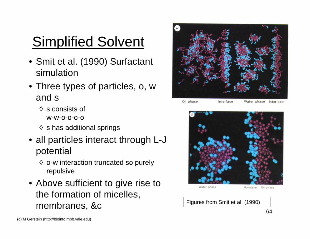
Simplified Solvent

Figures from Smit et al. (1990)

• Smit et al. (1990) Surfactantsimulation

• Three types of particles, o, wand s◊ s consists of

w-w-o-o-o-o

◊ s has additional springs

• all particles interact through L-Jpotential◊ o-w interaction truncated so purely

repulsive

• Above sufficient to give rise tothe formation of micelles,membranes, &c


Review -- Basic Forces• Basic Forces

◊ Springs --> Bonds

◊ Electrical

• dipoles and induced dipoles --> VDW force --> Packing• unpaired charges --> Electrostatics --> charge-charge

• Electrostatics◊ All described the PBE

◊ kqQ/r -- the simplest case for point charges

• Multipoles for more complex dist.• Validity of monopole or dipole Apx. (helix dipole?)

◊ Polarization (epsilon)

• Qualitative understanding of what it does• 80 vs 3


Review -- Simulation

• Moving on an Energy Landscape◊ Minimization -- steepest descent

◊ Monte Carlo◊ Molecular Dynamics

• Know how an atom will move◊ The problems

• Too complex --> Simplified Models• Potential Problems

• Analysis◊ Number density --> RDF, structural quantities

◊ Dynamic quantities, correlation functions, diffusion

• time course of variables◊ Hydrophobicity arises naturally in water simulation

• clathrate formation• high heat capacity, volume effects, &c.


Feedback

(S)imulation. (B)asic Forces (E)lectrostatics IIPreferred Lecture

counts

(1) too simple (2) just right (3) too complexLevel of Simulation

counts

(1) too simple (2) just right (3) too complexLevel of Basic Forces

counts

(1) too simple (2) just right (3) too complexLevel of Electrostatics II

counts


Feedbackon 2nd three computational lectures

• Which lecture did you like better(‘S’ for Simulation,‘B’ for Basic Forces,‘E’ for Electrostatics II)?

• Was the simulation lecture at right level(‘1’ for too basic, ‘2’ for just right, ‘3’ for too complex)?

• Was the basic forces lecture at right level(‘1’ for too basic, ‘2’ for just right, ‘3’ for too complex)?

• Was the electrostatics (II) lecture at right level(‘1’ for too basic, ‘2’ for just right, ‘3’ for too complex)?

• Sample responses: ‘S, 3, 2,1’ or ‘E-2-2-2’


Demos

• Minimization Demo◊ http://www.javasoft.com/applets/jdk/1.0/demo/GraphLayout/example2.html

• Adiabatic Mapping Demo◊ Molecular Motions Database

◊ http://bioinfo.mbb.yale.edu/MolMovDB

• Rotation Matrices, Rigid Body Motion Demo◊ 1swm, 2hbs, rasmol


References

• Allen, M. P. & Tildesley, D. J. (1987). ComputerSimulation of Liquids. Claredon Press, Oxford

• Brooks, B. R., Bruccoleri, R. E., Olafson, B. D.,States, D. J., Swaminathan, S. & Karplus, M.(1983). CHARMM: A Program for MacromolecularEnergy, Minimization, and Dynamics Calculations.J. Comp. Chem. 4, 187-217.

• Daggett, V. & Levitt, M. (1993). RealisticSimulations of Native-Protein Dynamics inSolution and Beyond. Ann. Rev. Biophys. Biomol.Struct. 22, 353-380.

• Dill, K. A., Bromberg, S., Yue, K., Fiebig, K. M.,Yee, D. P., Thomas, P. D. & Chan, H. S. (1995).Principles of protein folding--a perspective fromsimple exact models. Protein Sci 4, 561-602.

• Duan, Y. & Kollman, P. A. (1998). Pathways to aprotein folding intermediate observed in a 1-microsecond simulation in aqueous solutionScience 282, 740-4.

• Eisenberg, D. & Kauzmann, W. (1969). TheStructure and Properties of Water. ClarendonPress, Oxford.

• Franks, F. (Ed.) (1973). Water: A ComprehensiveTreatise. New York: Plenum Press.

• Franks, F. (1983). Water. The Royal Society ofChemistry, London.

• Gelin, B. R. & Karplus, M. (1979). Side-chaintorsional potentials: effect of dipeptide, protein,and solvent environment. Biochemistry 18, 1256-1268.

• Gerstein, M. & Chothia, C. (1996). Packing at theProtein-Water Interface. Proc. Natl. Acad. Sci.USA 93, 10167-10172.

• Gerstein, M. & Levitt, M. (1998). Simulating Waterand the Molecules of Life. Sci. Am. 279, 100-105.

• Gerstein, M. & Lynden-Bell, R. M. (1993a).Simulation of Water around a Model Protein Helix.2. The Relative Contributions of Packing,Hydrophobicity, and Hydrogen Bonding. J. Phys.Chem. 97, 2991-2999.

• Gerstein, M. & Lynden-Bell, R. M. (1993b). Whatis the natural boundary for a protein in solution? J.Mol. Biol. 230, 641-650.

• Gerstein, M., Tsai, J. & Levitt, M. (1995). Thevolume of atoms on the protein surface:Calculated from simulation, using Voronoipolyhedra. J. Mol. Biol. 249, 955-966.

• Hinds, D. A. & Levitt, M. (1992). A lattice modelfor protein structure prediction at low resolution.Proc Natl Acad Sci U S A 89, 2536-40.


References 2• Honig, B. & Nicholls, A. (1995). Classical

electrostatics in biology and chemistry. Science268, 1144-9.

• Karplus, M. & McCammon, J. A. (1986). Thedynamics of proteins. Sci. Am. 254, 42-51.

• Karplus, M. & Petsko, G. A. (1990). Moleculardynamics simulations in biology. Nature 347, 631-639.

• Levitt, M. (1982). Protein conformation, dynamics,and folding by computer simulation. Ann. Rev.Biophys. Bioeng. 11, 251-271.

• Levitt, M. (1983a). Molecular dynamics of a nativeprotein. I. Computer simulation of trajectories. J.Mol. Biol. 168, 595.

• Levitt, M. (1983b). Molecular dynamics of a nativeprotein. II. Analysis and Nature of the Motion. J.Mol. Biol. 168, 621-657.

• Levitt, M., Hirschberg, M., Sharon, R. & Daggett,V. (1995). Potential Energy Function andParameters for Simulations of the MolecularDynamics of Proteins and Nucleic Acids inSolution. Computer Phys. Comm. 91, 215-231.

• Levitt, M. & Sharon, R. (1988). AccurateSimulation of Protein Dynamics in Solution. Proc.Natl. Acad. Sci. USA 85, 7557-7561.

• McCammon, J. A. & Harvey, S. C. (1987).Dynamics of Proteins and Nucleic Acids.Cambridge UP,

• Park, B. H. & Levitt, M. (1995). The complexityand accuracy of discrete state models of proteinstructure. J Mol Biol 249, 493-507.

• Press, W. H., Flannery, B. P., Teukolsky, S. A. &Vetterling, W. T. (1992). Numerical Recipes in C.Second. Cambridge University Press, Cambridge.

• Pollack, A. (1998). Drug Testers Turn to'VirtualPatients' as Guinea Pigs. New York Times.Nov. 10,

• Press, W. H., Flannery, B. P., Teukolsky, S.A. & Vetterling, W. T. (1992). NumericalRecipes in C. Second. CambridgeUniversity Press, Cambridge.

• Sharp, K. (1999). Electrostatic Interactionsin Proteins. In International Tables forCrystallography, International Union ofCrystallography, Chester, UK.

• Sharp, K. A. & Honig, B. (1990).Electrostatic interactions inmacromolecules. Annu. Rev. Biophys.Biophys. Chem. 19, 301-32

• Smit, B., Hilbers, P. A. J., Esselink, K.,Ruppert, L. A. M., Os, N. M. v. & Schlijper(1990). Computer simulation of a water/oilinterface in the presence of micelles.Nature 348, 624-625.

Molecular Biophysics & Biochemistry 400a/700a (Advanced...

Documents

Transcript of Molecular Biophysics & Biochemistry 400a/700a (Advanced...