Molecular Astrophysics in Star-forming Regions with the...
71
THESIS FOR THE DEGREE OF LICENTIATE OF ENGINEERING Molecular Astrophysics in Star-forming Regions with the Odin Satellite CARINA M. PERSSON Department of Radio and Space Science CHALMERS UNIVERSITY OF TECHNOLOGY G¨ oteborg, Sweden 2006
Transcript of Molecular Astrophysics in Star-forming Regions with the...

THESIS FOR THE DEGREE OF LICENTIATE OF ENGINEERING
Molecular Astrophysics in Star-forming Regions
with the Odin Satellite
CARINA M. PERSSON
Department of Radio and Space ScienceCHALMERS UNIVERSITY OF TECHNOLOGY
Goteborg, Sweden 2006

Molecular Astrophysics in Star-forming Regionswith the Odin Satellite
CARINA M. PERSSON
c© Carina M. Persson, 2006
ISSN 1652 – 9103Technical Report No. 2006:17LRadio Astronomy & Astrophysics GroupDepartment of Radio and Space ScienceChalmers University of TechnologySE–412 96 Goteborg, SwedenPhone: +46 (0)31–772 1000
Contact information:
Carina M. PerssonOnsala Space ObservatoryChalmers University of TechnologySE–439 92 Onsala, Sweden
Phone: +46 (0)31–772 5537Fax: +46 (0)31–772 5590Email: [email protected]
Cover: An illustration of the Odin satellite, and part of a spectral scan towards theOrion KL region with the Odin satellite.
Printed by Chalmers ReproserviceChalmers University of TechnologyGoteborg, Sweden 2006

i
Molecular Astrophysics in Star-forming Regionswith the Odin SatelliteCARINA M. PERSSONDepartment of Radio and Space ScienceChalmers University of Technology
Abstract
The interstellar medium is the cradle of life, stars and planets in the evolving Universe.Stars are born deep inside cold and dark molecular clouds, and affect the dynamicalconditions in local regions by powerful winds, outflows, and by supernova explosions.Optical light from star-formation is trapped within the clouds because of absorptionby dust grains. However, radiation is able to escape through the gas and dust in theinfrared and radio spectral regions. In addition, the chemical evolution of moleculesis very sensitive to temperature, density and radiation field. Thus, radio and submmobservations of molecules are an excellent probe of both the physical and chemicalconditions in star-forming regions and the interstellar medium in general.Some important molecules are difficult to observe with ground-based telescopes dueto the Earth’s obscuring atmosphere. Hence observations from space are necessary inthese spectral regions. The launch of the Odin1 satellite in 2001, enabled observationsof molecular oxygen and the ground-state water transition that traces shocks and star-formation.One of the big unanswered questions in astronomy is the origin of structure. Duringthe cosmic Dark Ages after the Big Bang, the Universe evolved from uniformity to thestructures of galaxies, clusters, and voids that we observe today. Direct observationsfrom the Dark Ages are most commonly believed to be impossible. But our aim in thesearch for the Primordial molecules is exactly this – to perform observations of resonantspectral lines from the cosmic Dark Ages.To study the conditions in a star-forming region, including an unbiased search for newmolecules, a spectral line survey has been performed toward the Orion KL massivestar-forming region. We have observed 347 spectral lines from 38 molecules includingisotopologues, while 19% of the lines remain unidentified. Six water lines are detectedincluding the water isotopologues H17
2 O, H182 O and HDO. The total emission is domi-
nated by CO, H2O, SO2, SO, 13CO and CH3OH. Species with the largest number of linesare CH3OH, (CH3)2O, SO2, 13CH3OH, CH3CN and NO.
Keywords: ISM: abundances – ISM: molecules – Astrobiology – Molecular data – ISM:individual objects: Orion KL – Radio lines: ISM – Submillimeter – line: formation –line: identification
1Odin is a Swedish-led satellite project funded jointly by the Swedish National Space Board (SNSB), theCanadian Space Agency (CSA), the National Technology Agency of Finland (Tekes) and Centre Nationald’tudes Spatiales (CNES). The Swedish Space Corporation was the prime contractor and also is responsiblefor the satellite operation.

ii

iii
Research contributions
This thesis is based on the work reported in
• Paper I: A.O. Henrik Olofsson, Carina M. Persson, N. Koning, T.I. Hasegawa,P. Bergman, P. Bernath, J. Black, U. Frisk, W. Geppert, A. Hjalmarson, S. Kwok,B. Larsson, A. Lecacheux, A. Nummelin, M. Olberg, Aa. Sandqvist, and E.S. Wirstrom:A spectral line survey of Orion KL from 486-492 and 541-577 GHzwith the Odin satellite. I. The DataTo be submitted to Astronomy & Astrophysics
• Paper II: Carina M. Persson A.O. Henrik Olofsson, N. Koning, T.I. Hasegawa,P. Bergman, P. Bernath, J. Black, U. Frisk, W. Geppert, A. Hjalmarson, S. Kwok,B. Larsson, A. Lecacheux, A. Nummelin, M. Olberg, Aa. Sandqvist, and E.S. Wirstrom:A spectral line survey of Orion KL from 486-492 and 541-577 GHzwith the Odin satellite. II. Data analysisTo be submitted to Astronomy & Astrophysics
and
• Searches for Primordial molecules from the Early Universe:Carina M. Persson, P. Encrenaz, A. Hjalmarson, M. Olberg, and G. Rydbeck.Chapter 3 and:Encrenaz, P., Persson, C.M., Hjalmarson, A, de Bernardis, P., Chambaud, G., Daniel, J.Y.,Frisk, U., Maoli, R., Masi, S., Melchiorri, B., Melchiorri, F., Olberg, M., Pagani, L.,Rosmus, P., Rydbeck, G., Sandqvist, Aa., and Signore, M.Progress in searches for primordial resonant lines using the Odin satelliteIAUS, 231, 241 (2005)

iv

5
Acknowledgements
There are a few people that I want to mention especially. First of all — I am verygrateful to my supervisor Michael Olberg who has been the very best supervisor forme. And many thanks to my assistant supervisor Ake Hjalmarson whose encourage-ment is very appreciated, to John Black for his kindness and knowledge, and to PerBergman, Gustaf Rydbeck, and Roger Hammargren who always are very helpful. Andwhat would I have done without my special friend Eva, and Henrik, Paula, Susanne,Julia, Vivi, Margareta, Ingrid, Cathy, Monica, Eva N, Eva A, Camilla, Raquel, and allcolleagues and staff members at Onsala and the whole Astronomy and Astrophysicsgroup. Thanks also to the former head of the observatory Roy Booth, to the new, HansOlofsson, and to Pierre Encrenaz from Observatoire de Paris.To all my friends and teachers at the University of Uppsala, Leif Karlsson at the Physicsdepartment, and especially the Astronomy department and the Galaxy group includingNils Bergvall, Erik Zackrisson, and Kjell Olofsson, as well as Kjell Eriksson and BengtEdvardsson – thanks a lot for your encouragement. And also many thanks to JohannesOrtner, director for the Alpbach Summer School, Austria.And to my family – my wonderful, lovely, best of all children! Andreas, Anna, Maria,och Rebecca. Tack for att ni alltid ar de basta barnen som finns! Och tack! mamma ochpappa och min moster Anita for all hjalp. And to Felicia, and to you Kaj, who have myheart.I am grateful to the Swedish National Space Board (SNSB) for support of this PhDproject.
Carina

I also participated as a co-investigator in the following papers
• Wirstrom, E.S., Bergman, P., Olofsson, A.O.H., Frisk, U., Hjalmarson, A., Olberg, M.,Persson, C.M., and Sandqvist, Aa.,Odin CO and 13CO J = 5 – 4 mapping of Orion KL – a step towards accurate waterabundancesAstronomy & Astrophysics, 453, 979 (2006)
• Wilson, C.D., Booth, R.S., Olofsson, A.O.H., Olberg, M., Persson, C.M., Sandqist, Aa.,Buat, V., Encrenaz, P.J., Fich. M., Frisk, U, Gerin, M., Johansson, L.E.B., Rydbeck, G.,and Wiklind, T.Upper limits to the water abundance in starburst galaxiesSubmitted to Astronomy & Astrophysics
• Berciano Alba, A., Borges da Silva, P., Eichelberger, H, Giovacchini, F, Godolt, M.,Hasinger, G., Lerchster, M., Lusset, V., Mattana, F., Mellier, Y., Michalowski, M.,Monteserin-Sanches, C., Noviello, F., Persson, C.M., Santovincenzo, A., Schneider, P.,Zhang, M., and Ostman, L.DEMON: a Proposal for a Satellite-Borne Experiment to study Dark Matter andDark Energyastro-ph/0606010Accepted for publication in the SPIE conference proceedings (2006):Space Telescopes and Instrumentation II: Ultraviolet to Gamma Ray (AS02)Part of SPIE’s International Symposium on Astronomical Telescopes and Instru-mentation

Contents
Abstract . . . . . . . . . . . . . . . . . . . . . . . . . . . . . . . . . . . . . . . . . i
Research contributions . . . . . . . . . . . . . . . . . . . . . . . . . . . . . . . . iii
Acknowledgements . . . . . . . . . . . . . . . . . . . . . . . . . . . . . . . . . . 5
1 The Interstellar Medium 1
1.1 Introduction . . . . . . . . . . . . . . . . . . . . . . . . . . . . . . . . . . . 1
1.2 Dust grains and ices . . . . . . . . . . . . . . . . . . . . . . . . . . . . . . 2
1.3 Astrochemistry . . . . . . . . . . . . . . . . . . . . . . . . . . . . . . . . . 4
1.3.1 Water . . . . . . . . . . . . . . . . . . . . . . . . . . . . . . . . . . . 8
1.4 Molecular environments . . . . . . . . . . . . . . . . . . . . . . . . . . . . 10
1.4.1 HII regions . . . . . . . . . . . . . . . . . . . . . . . . . . . . . . . . 11
1.4.2 Photodissociation or Photon Dominated Regions . . . . . . . . . 11
1.4.3 Hot cores . . . . . . . . . . . . . . . . . . . . . . . . . . . . . . . . . 12
1.4.4 Shocks and outflows . . . . . . . . . . . . . . . . . . . . . . . . . . 13
1.4.5 Cold dark clouds . . . . . . . . . . . . . . . . . . . . . . . . . . . . 13
1.4.6 Giant Molecular Clouds (GMCs) . . . . . . . . . . . . . . . . . . . 13
2 Star-formation 15
2.1 Jeans mass and star-formation . . . . . . . . . . . . . . . . . . . . . . . . . 15
2.2 Heating and cooling . . . . . . . . . . . . . . . . . . . . . . . . . . . . . . 16
2.3 The first stars . . . . . . . . . . . . . . . . . . . . . . . . . . . . . . . . . . 18
3 Searches for Primordial Molecules in the Early Universe 19
3.1 The beginning . . . . . . . . . . . . . . . . . . . . . . . . . . . . . . . . . . 19
3.2 Elements of our primordial medium . . . . . . . . . . . . . . . . . . . . . 21
3.3 Resonant scattering . . . . . . . . . . . . . . . . . . . . . . . . . . . . . . . 23
3.4 Implications . . . . . . . . . . . . . . . . . . . . . . . . . . . . . . . . . . . 25
3.5 Observations . . . . . . . . . . . . . . . . . . . . . . . . . . . . . . . . . . . 25
3.5.1 Previous observations . . . . . . . . . . . . . . . . . . . . . . . . . 25
3.5.2 Our Odin observations . . . . . . . . . . . . . . . . . . . . . . . . . 26
3.6 Future prospects . . . . . . . . . . . . . . . . . . . . . . . . . . . . . . . . . 28
7

8 CONTENTS
4 Introduction to Paper I and Paper II 29
4.1 The Odin satellite . . . . . . . . . . . . . . . . . . . . . . . . . . . . . . . . 294.2 The Orion nebula . . . . . . . . . . . . . . . . . . . . . . . . . . . . . . . . 304.3 Summary of Paper I and Paper II . . . . . . . . . . . . . . . . . . . . . . 33
Paper I 37
Paper II 61
Abstract of poster 109
A Tools of astronomy 113
A.1 Radiative transfer . . . . . . . . . . . . . . . . . . . . . . . . . . . . . . . . 113A.1.1 Optical depth and source function . . . . . . . . . . . . . . . . . . 114A.1.2 Solution of the transport equation . . . . . . . . . . . . . . . . . . 115A.1.3 Special cases . . . . . . . . . . . . . . . . . . . . . . . . . . . . . . . 116A.1.4 Discrete processes – spectral line theory . . . . . . . . . . . . . . . 118A.1.5 Photon creation, destruction, scattering and conversion . . . . . . 120A.1.6 Types of equilibrium . . . . . . . . . . . . . . . . . . . . . . . . . . 121A.1.7 Critical density . . . . . . . . . . . . . . . . . . . . . . . . . . . . . 122
A.2 Radioastronomy . . . . . . . . . . . . . . . . . . . . . . . . . . . . . . . . . 123A.3 Column densities . . . . . . . . . . . . . . . . . . . . . . . . . . . . . . . . 124
A.3.1 Rotational diagram . . . . . . . . . . . . . . . . . . . . . . . . . . . 125
Bibliography 127

Chapter 1
The Interstellar Medium
1.1 Introduction
A galaxy consist of billions of stars, and in between there is an important con-stituent of gas and dust particles called the Interstellar Medium (ISM). Of allvisible matter in our Galaxy approximately 15% is composed of interstellar gasand dust. We observe this very dilute gas by its own emission and by the ab-sorption of starlight that travels trough it.
The ISM might at first glance seem uninteresting, but there are a numberof reasons to study it. First, it all starts here. The Universe is continuouslyevolving, and the stars are born deep within cold molecular clouds. By studyingthe ISM we gain information about the necessary conditions for star-formation.
When the stars end their lives (in different ways depending on their initialmass) they return most of the gas to the ISM. Gas is also lost by the stars duringtheir entire lifetimes in stellar winds. Almost everything in the Universe is thusrecycled. But when the gas is returned to the ISM, the composition is not thesame anymore. After the Big Bang the primordial composition of the ISM wasabout (by mass) 75% of hydrogen and 25% of helium. Today most of the ISMstill has approximately this composition, but now there are other heavier ele-ments as well, especially in the dust. The elements have been processed withinthe hot cores of stars in different nucleosynthesis processes, where the hydrogennuclei are combined into helium in the proton-proton chain or CNO-cycle, he-lium nuclei combine into carbon or oxygen in the triple alpha process, etc. Ele-ments heavier than iron can only be produced when very massive stars explodeas supernovas. Thus, early generation stars contained (almost) only hydrogenand helium, while the next generation of stars, and their possible solar systems,contained all other elements produced by the previous stars. So by studying therelative elemental abundances of the ISM, we can obtain information about thechemical evolution in our Galaxy, and the history of star-formation includingdifferent types of supernovae.
1

2 The Interstellar Medium
The ISM is also a unique chemical laboratory characterised by very low den-sities and temperatures (typically a few tens of Kelvins) not available on Earth,allowing studies of chemistry otherwise not accessible. For instance the radicalHCO+ was first observed in the ISM and only later observed and confirmed inthe laboratory (summary is given in Rydbeck & Hjalmarson 1985).
Another example of the importance of studies of the ISM is deuterium ob-servations. Since no efficient processes of deuterium (isotope of hydrogen) pro-duction are known, almost all existing deuterium today is a relic from the BigBang. If we measure the primordial abundance of deuterium in the local orextra-galactic ISM, a limit on the primordial value of the relative abundance of[D/H] can be obtained. This value is used to calculate the baryonic density inthe Universe, thus constraining the Big Bang Nucleosynthesis.
The ISM is not a homogeneous gas cloud with equal density and temper-ature spread evenly throughout the Galaxy. Our Galaxy, the Milky Way, con-tains ∼4–8×10⁹ M¯ of neutral hydrogen, and about half of that amount existas molecular hydrogen. Almost all of the molecular gas is piled up in a ring 4kpc from the centre of the Milky Way. The neutral gas is found across the wholeGalaxy. The sizes of the clouds range from 0.1 pc for dark, isolated cloudlets tomore than 10 pc for Giant Molecular Cloud complexes. The density is typicallyhigher in the spiral arms and towards the centre, and can vary by many ordersof magnitude – from less than 1 particle per cm−3 to 107 cm−3 in dense clouds– while the temperature variation is smaller (from tens of K to millions of K).To get a feeling for what a dense medium in space means we can compare thiswith the best vacuum on Earth, which has a density of 106 cm−3, or the air atsea level with a density of 3×1019 cm−3.
On small scales (. 1 kpc) the ISM forms a multi-phase medium with dif-ferent co-existing phases. Low density gas with high temperature is in pres-sure equilibrium with higher density, lower temperature gas. A warm, diffusemedium with a temperature of about 8 000 K corresponds to a density of ∼0.1cm−3, while colder gas of 100 K corresponds to a density of 10 cm−3. The evendenser molecular clouds are gravitationally bound entities. A hot plasma phasealso exists with a temperature of 106 K, and a number density of 10−3 cm−3.Most of the mass is in the dense phase, but the diffuse plasma occupies most ofthe volume. The gas material passes continuously between the different phases.
1.2 Dust grains and ices
In addition to the gas the ISM contains approximately ∼1% (by mass) of smalldust particles (0.01µm-1µm) consisting of solid state molecules heavier than hy-drogen, such as silicates, graphite, amorphous carbon (soot), and polycyclic aro-matic hydrocarbons (PAHs). The bulk of the dust grains originates in oxygen-

1.2 Dust grains and ices 3
rich M giants (silicate dust), radio-luminous OH/IR stars, super-giants, and car-bon stars (sooty particles). They form near the photosphere of the star togetherwith molecules and radiation pressure on the grains drives the circumstellarwind, which injects the dust and gas into the ambient ISM. Supernova shockwaves distribute the dust over large scales, and the dust is subsequently mixedinto the ISM.
Dust particles can absorb and scatter photons, and this shields the interiorparts of a cloud enabling molecules to survive. The absorption of radiationheats the grains to radiate in infrared, i.e. they can absorb uv- and visible lightand transform the radiation to longer wavelengths. The absorption of UV pho-tons also causes electrons to be ejected from the grains, which is an importantheating source of the gas.
Many gas-phase reactions demand a ”starter” molecule. This can be pro-vided by molecular formation on the surface of dust grains, where a complicatedchemistry is occurring including (almost) all of the H2 production. The forma-tion rate primarily depends on the nature of the grain surface, which creates anenvironment to prolong the collision time of the elements, and hence the proba-bility for a reaction to occur increases. At 10 K the H, D, C, O and N atoms havesufficient mobility to scan the grain surface to find a reaction partner.
In colder regions the surface is often covered with a layer of volatile material.This is typically ices of H2O, CH3OH, CO2, CO, CH4, NH3, and OCS. H2O is thedominant species and CO2 is the second most common with about 20 percent ofthe water abundance. However, in the gas-phase CO2 is surprisingly rare. Thedust particles can acquire these icy grain mantles through the slow, but efficient,accretion of species in the gas-phase. The sticking coefficients are expected to beclose to unity for heavy species at low temperatures. The time for removal fromthe gas-phase to the dust is about 3×10⁹/nH years, where nH is the hydrogennucleon number density. With a density of 104 cm−3, the depletion time scaleis only about 3×10⁵ years, which is less than the expected lifetime of densecores in GMCs (see section 1.4.6). Icy grain mantles have been observed withSWS (Short Wavelength Spectrometer) on-board the ISO-satellite between 2.5and 200 µm (Gibb et al. 2004).
In the amorphous ice on the grain surfaces a complex chemistry is takingplace. On Earth atoms and organisms demand liquid water to be able to formlarger species. But at the cold temperatures present in space, the water will be inthe form of ice. The water molecules are then ordered in a rigid crystalline struc-ture and this recoils other species. However, in vacuum, cold water moleculesbehave differently and produce an amorphous ice, which has similar propertiesto liquid water. The hydrogen bonds between the water molecules redistributeconstantly and rapidly, and this creates an excellent environment for moleculesto form. As much as 10 percent of the water volume can consist of other species.
The molecules get off the dust grains by different methods: sputtering in

4 The Interstellar Medium
shocks, X-ray or UV-radiation, thermal desorption, cosmic rays, or chemicalenergy of reactions (H2).
1.3 Astrochemistry
In radio and sub-mm astronomy we mainly observe the low-energy rotationalmolecular transitions from molecular clouds that are too cold to radiate in theinfrared or visible regions of the spectrum. Molecules influence the birth anddistribution of stars and structure of galaxies, and the entire cosmos is on thelarge scale chemically controlled. Radio astronomy and the study of moleculesare therefore important parts of astronomy in general. Molecular astrophysicsbegan with the discovery of CH, CH+, and CN in the late 1930s. The first obser-vation demonstrating the existence of dense star-forming gas was the detectionof the ammonia J = 1, K = 1 inversion line in 1968 (Cheung, Rank and Townes)towards the Galactic Centre. The observed lines also made a temperature es-timation possible, and also showed that polyatomic interstellar molecules didexist.
Astrochemistry is the study of interstellar molecules, their formation routesand the use of these species to gain information about the ISM. Since the spaceoffers low density and temperature, highly reactive, chemically unstable specieson Earth can therefore be quite abundant in certain regions. These include ionslike HCO+, and radicals like OH, CH and CN, which are electrons with un-paired electrons. But the overwhelmingly most abundant molecule in the ISMis H2 (99.99% of all molecules). As a consequence of no allowed dipole transi-tions in the symmetric H2, most of the contents in cold molecular clouds is thusinvisible. Molecular hydrogen can only be seen in infrared, through vibrational-rotational transitions, in most cases tracing the hot gas. To be able to trace thecold H2 gas, the second most common molecule CO, with an abundance rela-tive to H2 of ∼10−4, is used assuming co-spatial existence. CO is easily excitedat modest densities and temperatures and is very tightly bound. HI is observedin the hyperfine transition at 21 cm (1420 MHz), which is a low-probability tran-sition in the ground energy level, when the electron changes its spin relative tothe proton. Other detected molecules are very familiar to us like water, ammo-nia and formaldehyde.
Around 150 molecules have been detected in space as seen in Table 1.1. Com-pounds of the elements with the highest abundances, hydrogen, carbon, oxy-gen, and nitrogen, constitute the major part of the detected molecules. Moleculesthat form from heavier refractory elements, such as S, Si or Mg, often reside inthe dust particles. Larger carbon-bearing species like polycyclic aromatic hy-drocarbons, PAHs, may also be present in ISM.

1.3 Astrochemistry 5
Table 1.1: Detected interstellar molecules as of October 2006, (149+). Cyclic form islabelled c-, and linear form with l-. A question mark is added to a not confirmed detec-tion. Credit: Ake Hjalmarson.
Hydrogen compounds Oxygen
H a2 HD a H+
3 H2D+ O2
Hydrogen and Carbon compounds
CH b CH+ a C a2 CH2 C2H
C3 CH3 C2H d2 l-C3H c-C3H
CH d4 C4 c-C3H2 l-H2CCC C4H
C c5 C2H c
4 C5H l-H2C4 HC4H c
CH3C2H C6H HC6H c H2C6 C7H c
CH3C4H CH3C6H C8H C6H c6
Hydrogen, Oxygen and Carbon compounds
OH b d CO b d CO+ d H2O d HCO
HCO+ d HOC+ C2O CO2d H3O+ d
HOCO+ H2CO d C3O CH2CO HCOOH d
H2COH + CH3OH d CH2CHO CH2CHCHO HC2CHOC5O CH3CHO c-C2H4O CH2CHOH c-C3H2O
CH3OCHO d CH3COOH CH2OHCHO (CH3)2O CH3CH2OH
CH3CH2CHO (CH3)2CO HOCH2CH2OH d C2H5OCH3 (CH2OH)2CO ?
Hydrogen, Nitrogen and Carbon compounds
NH a ,d (ND?) CN b ,d N a2 NH a ,d
2 HCNd
HNCd N2H+ NHd3 HCNH+ H2CN
HCCN C3N CH2CN CH2NH HC2CNd
HC2NC NH2CN C3NH CH3CNd CH3NCHC3NH+ HC4Nc C5N CH3NH2 CH2CHCNHC5N HC7N HC9N HC11N CH3CH2CNCH3C3N CH2CCHCN CH3C5N c-C2H4NH ? CH2CNH
Hydrogen, Nitrogen, Oxygen and Carbon compounds
NO HNO N2O HNCOd NH2CHOd
CH3CONH2 NH2CH2COOH?
Other species (containing S, Si, Na, K, Cl, F, Al, Mg, Fe, P)
SH CSd SOd SO+ NSSiH SiCc SiN SiO SiSHCl NaClc AlClc KClc HF
AlFc CPc PN H2Sd C2S
SOd2 OCSd HCS+ c-SiC2 SiCNc
SiNCc NaCNc MgCNc MgNCc AlNCc
H2CSd HNCS C3S c-SiC3 SiH4c
SiC4c CH3SH C5S FeO CF+
Polycyclic Aromatic Hydrocarbons (PAHs)
a Detected in visible/UV absorption. bDetected in visible/UV absorption, and inradio. cOnly circumstellar species. dAlso detected in comets.

6 The Interstellar Medium
There are a number of different routes to the production of molecules, whereone major formation process occurs on the surface of dust grains. The problemof gas-phase reactions is one of energetics. When two atoms collide then cannotform a bound system unless energy can be removed, for instance in a simulta-neous collision of a third atom or by emission of a photon during the collision.Otherwise the atoms will merely bounce off each-other. On Earth the densityis very high and molecules form easily in three-body collisions. In space thedensity is too low for this process to occur efficiently, except in the circumstel-lar envelopes of cold, late-type, post-AGB stars, which offer a warm and denseenvironment giving a rich chemistry. As seen in Table 1.1 some molecules suchas C5, C7H, and HC6H among others are only detected in these regions.
Since no three-body collisions occur in the ISM, instead efficient ion-moleculereactions drive most of the interstellar chemistry, and in high temperature gas itis neutral-neutral reactions. The colliding species can be atoms or molecules. Theneutral-neutral reactions typically have energy barriers of the order of ∼100 K,and are only about 1 per cent as likely to occur as are ion-molecule reactionsat low temperatures. With increasing temperature the reactions become moreefficient. Thus a rich gas-phase chemistry needs warm gas or the presence ofions, which are produced by cosmic rays (relativistic protons or electrons), orUV-radiation from nearby hot, young stars. The most important ion is H+
3 whichstarts most other reactions.
Molecules can also be produced by radiative association, when the energy sinkis a photon. Two atoms collide and form an excited molecule which radiativelydecays to the ground state before it dissociates. But the probability is generallyvery low for these reactions to occur.
Destruction of molecules occurs by different processes, such as dissociative re-combination. An ambient free electron recombines with a molecular ion and cre-ates an energetic, unstable neutral molecule. The molecule can autoionize again,losing the electron, or fall apart into its neutral species. This reaction increasesslowly as the temperature falls. An illuminating case is the reaction H3O+ + e−,which forms more OH + 2 H than H2O + H. Another destruction source is ener-getic radiation. Molecules do not in general survive if the temperature is aboutten times hotter than in the Earth’s atmosphere. In dense regions very com-plex molecules can be produced since the outer layer of the cloud is an effectiveshield against the UV radiation. But if the clouds are diffuse, the incoming UVphotons destroy larger molecules faster than their production, so only small andsimple molecules can survive. Some molecules like H2 and CO protect them-selves with self-shielding. This is possible since the destruction process occurs ina number of very narrow spectral bands. The radiation outside these bands
does not affect the molecule. CO is also shielded by H2.
Diagnosis of molecular clouds depends on molecular physics. An atom ormolecule absorbs and emits radiation at wavelengths that are characteristic of

1.3 Astrochemistry 7
Figure 1.1: Energylevel diagrams of O2, CI, 13CO and o-H2O. Credit: Gary Melnick.
the species. The energy level diagrams of O2, CI, 13CO and o-H2O in Fig. 1.1show some of the lowest rotational transitions within the first vibrational statefor each species. The transitions observed with the SWAS satellite are marked.The Odin satellite observe all these lines, and more. The magnetic dipole transi-tion 11 – 10 of O2 at 118.750 GHz is Odin’s most sensitive search tool. Molecularoxygen has been shown to be orders of magnitude less abundant than expectedfrom chemical models (Pagani et al. 2003), and just has been marginally de-tected in the dense molecular core ρ Oph A (Liseau et al. 2005).
An object may appear different in different transitions of the same moleculeor in lines of different species. This is a consequence of the response by themolecules to the physical conditions in the medium, including temperature,

8 The Interstellar Medium
abundance, and the background radiation, and this determines the strength ofthe spectral features of the species. Some molecules have very high critical den-sities, e.g. CN or CS. Thus these species radiate most strongly when the densityis high, and are therefore excellent tracers of high-density gas. Other moleculessuch as CO have a low critical density and are easily observed from large re-gions. The excitation temperature can be directly determined by observing anoptically thick transition, whereas the column density is derived from opticallythin transitions (appendix A).
1.3.1 Water
The water molecules is of special interest for a number of reasons – first as a keymolecule for life as we know it (Brack 2002). The origin of water in the ISM andhow it is connected to star-formation is of clear astrobiological interest. Water isalso an important ice constituent on the surface of dust grains, and provides anexcellent environment to form and shield molecular production. It also helpsthe coagulation process that produces planets and comets, which are formedby grains, rocky debris, and ices. Like planets, comets must form around otherstars than our sun, as in fact suggested by Odin’s detections of H2O and NH3
in the mass-loss winds from the C-rich star IRC+10216 and the O-rich star WHya (Hasegawa et al. 2006). Their delivery of volatiles to the planets via aheavy bombardment, as in the case of our young Earth, may be important forthe formation of oceans and atmospheres and the life itself. In addition, water isvital to the understanding of oxygen chemistry, and also an important coolingagent in warm star-forming regions, where the abundance is relatively high(read more in chapter 2.2).
In 1969, Cheung et al. detected water emission for the first time in a highenergy maser amplifying transition, towards three sources – the Orion Neb-ula, Sgr B2 and W49. But due to the Earth’s atmosphere which is completelyopaque around the strongest transitions, it is necessary to perform observationsfrom space-borne satellites. The ISO satellite, operational between November1995 and May 1998, observed water at wavelengths from 2.5 to 240 µm (in-frared spectral region) and measured the water abundance both in vapour andsolid form (review in Cernicharo & Crovisier 2005). The Spitzer Space Telescopewas launched August 2003, on a 2.5-year mission, to obtain images and spectrabetween wavelengths of 3 and 180 µm. The SWAS satellite, launched in Decem-ber 1998 and operating during 5.5 years, performed extensive, simultaneousobservations of the rotational ground state transition of gas-phase o-H2O, 13COJ = 5 – 4, and CI 3P1 – 3P0 lines in thousands of lines-of-sight. The Odin satellite(see Sect. 4.1), launched a few years later in 2001, was a more sensitive next stepafter SWAS, and continued the observations of rotational ground state water aswell of its important isotoplogues.

1.3 Astrochemistry 9
The results of all these observations indicate that the water abundance rela-tive to molecular hydrogen is low in the gas-phase of dark cold clouds, about10−8–10−9, where it mostly (98%) resides in the ices on the dust grains. Inshocked gas and warm star-forming regions, where water is released from theices on dust grains and effective chemical reactions produce large amounts ofwater, high gas-phase abundances of about 10−4–10−5 are observed.
Water can be formed in three different ways. At low temperatures the majorroute of gas-phase production is the neutral-ion process and involves a chain ofhydrogen-abstraction reactions terminated by dissociative recombination:
H+
3 + O → H2 + OH+
OH++ H2 → OH+
2 + HOH+
2 + H2 → H3O++ H
H3O++ e− → H2O + H
The gas-phase neutral-neutral reaction is efficient at temperatures above 400 K,with the major sequence:
H2 + O + 2 980 K → OH + HOH + H2 + 1 490 K → H2O + H
where the temperatures involved are the energy barriers. In warm gas nearlyall the available oxygen is converted into water due to these fast reactions, ona timescale of about one hundred years, and produces about 100 times morewater than the neutral-ion process is able to.
The third path of water production is grain surface hydrogenation and pro-duces large amounts of water ice on the dust grains, which is believed to be amajor reservoir of oxygen. At temperatures above 90 K this ice can sublimate togas-phase water.
Figure 1.1 shows the lower part of the ortho-H2O energy level diagram. Anortho and para H2O energy level diagram including much higher energy statescan be found in Rydbeck & Hjalmarson 1985). The rotational ground state tran-sition 11,0–10,1 at 557 GHz is marked, as well as other important molecular linesobserved by the Odin satellite. Asymmetric tops with identical hydrogen nu-clei, like water, are for symmetry reasons divided into two subspecies calledortho and para states. The dipole selection rules allow the rotation quantumnumber J to change by 0 or ±1, while the quantum numbers K−1 or K+1 canchange by ±1 or ±3. The states with even K−1 and odd K+1 are called orthostates, and vice versa for the para states. No transitions between the ortho andpara states are allowed. The degeneracy is three times greater for the orthostates, owing to the nuclear spin statistical weights of the hydrogen nuclei.
Water has a relatively large dipole moment, and this implies that many tran-sitions have large A-coefficients (read more in Appendix A). Higher levels are

10 The Interstellar Medium
therefore difficult to populate collisionallly. The rotational ground state transi-tion 11,0–10,1 of ortho-H2O has A-coefficient 3.5×10⁻³ s−1. With a collisional de-excitation rate of 2.0×10⁻¹⁰ cm−3 s−1 at a kinetic temperature of 20 K, the criticaldensity is 2×107 cm−3. Most molecular clouds have densities much less thanthis. At low densities the water rotational levels can still be excited by infraredcontinuum photons from heated dust grains. Due to the large A-coefficient theoptical depth (Appendix A) will be very high for many transitions includingthe ground state rotational transition observed by the Odin satellite.
The high optical depth of the o-H2O line precludes a correct abundance esti-mation. As substitutes, observations of the optically thin o-H17
2 O and the almostoptically thin o-H18
2 O transitions are used for column density and abundancedeterminations (details in Appendix A).
1.4 Molecular environments
There are many different molecular environments in the ISM, with distinctivechemical characteristics and intimately linked to the formation and evolution ofstars. During a star-formation process the chemical state of the region will bemodified by the increasing temperature of young embedded stars (from 10 Kto a few 100 K), outflows and shocks that can elevate the temperature locally tomore than 2000 K. This high temperature changes the chemical reactions, andalso returns material to the gas-phase from the icy dust grains through evapora-tion. The evaporated species can have been formed previously in the gas-phaseand then frozen out onto the dust grains, or through chemical reactions on thesurface of dust grains, e.g. the H2 molecule. Cold gas-phase chemistry can eas-ily produce simple species such as CO, N2, C2H2, C2H4 and HCN, and othersimple carbon chains. These molecules can later condense onto dust grains,where subsequent reactions produce such species as CH3OH and CO2. Subli-mation releases the molecules back to gas-phase, where they in turn can act asprecursors for larger species.
The transformation of chemical composition in a protostellar nebula will besmall in the outer cooler part, but in the inner warm part a major reprocessing ofgrains and molecules will occur. One important question concerns how muchof the organic material present in comets is pristine interstellar material, and towhat extent it has been processed within the nebula from it was formed.
Close to stars radiating in ultraviolet, the gas will be ionised in HII regions.Farther away there will be a transition region between the ionised gas and thecold and dense cloud, a Photo Dissociation Region (PDR). Shocks and outflowsproduced by a new-born or a dying star, as well as Hot Cores also play im-portant roles in astrochemistry. All these regions represent different stages inthe star-formation history. The abundance and distribution of molecules will

1.4 Molecular environments 11
probe these different environments. If the chemical evolution of molecules canbe understood, they can trace these specific physical activities in the protostel-lar environment, so that our understanding of star-formation increases. Thisis done by comparing observations with experimental data and detailed, verycomplex modelling, taking into account thousands of chemical reactions andreaction rates.
However, the reverse is also true – the initial molecular abundances and levelof ionisation affect the star-formation process, including the rate of collapse, andthe efficiency of star-formation in the cloud (see chapter 2). Hence the chemistrycontrols the evolution of molecular clouds and stars, and is a diagnostic of thephysical conditions in them.
A short summary follows for a few different molecular environments whichare relevant for the research presented in later sections.
1.4.1 HII regions
Massive and very hot newly-formed O or B-stars radiate large amounts of ul-traviolet radiation (hν >13.6 eV), and dissociate and ionise the surroundingmolecular and neutral hydrogen isotropically. These fully ionized clouds aresignposts of massive star formation and their distribution across our Galaxy in-dicates that the formation of massive stars is concentrated in the spiral armsof dense gas. The gas is heated to temperatures around 10 000 K, which willcause the hydrogen to emit radiation in visible light. Another name is emissionnebulae. One of the best studied examples is the Orion Nebula.
An HII region can be quite large. A star of spectral type O can ionise a regionup to hundreds of parsecs in diameter (depends on the density of the star),while a B star will produce a few parsec region. However, these luminous andvery massive stars cannot maintain the UV flux for more than a few millions ofyears, since they have rather short lifetimes.
1.4.2 Photodissociation or Photon Dominated Regions
Farther away from a luminous UV-radiating massive star, when the photonshave energies between 6 and 13.6 eV (FUV photons), there is a transition zonecalled photo dissociation region (PDRs) between the ionised HII region, andthe dark cold molecular cloud. The FUV photons dominate the physical andchemical processes in a PDR, thus a large portion of the gas in the ISM residesin PDRs. The structure is determined by the density and the intensity of theincident FUV radiation field.
Most high-energy photons are absorbed by the dust and molecules in theouter layers of the PDR, but a small fraction is able to heat the gas by the photo-electric effect to a few hundred K, and to ionise atoms and to dissociate the
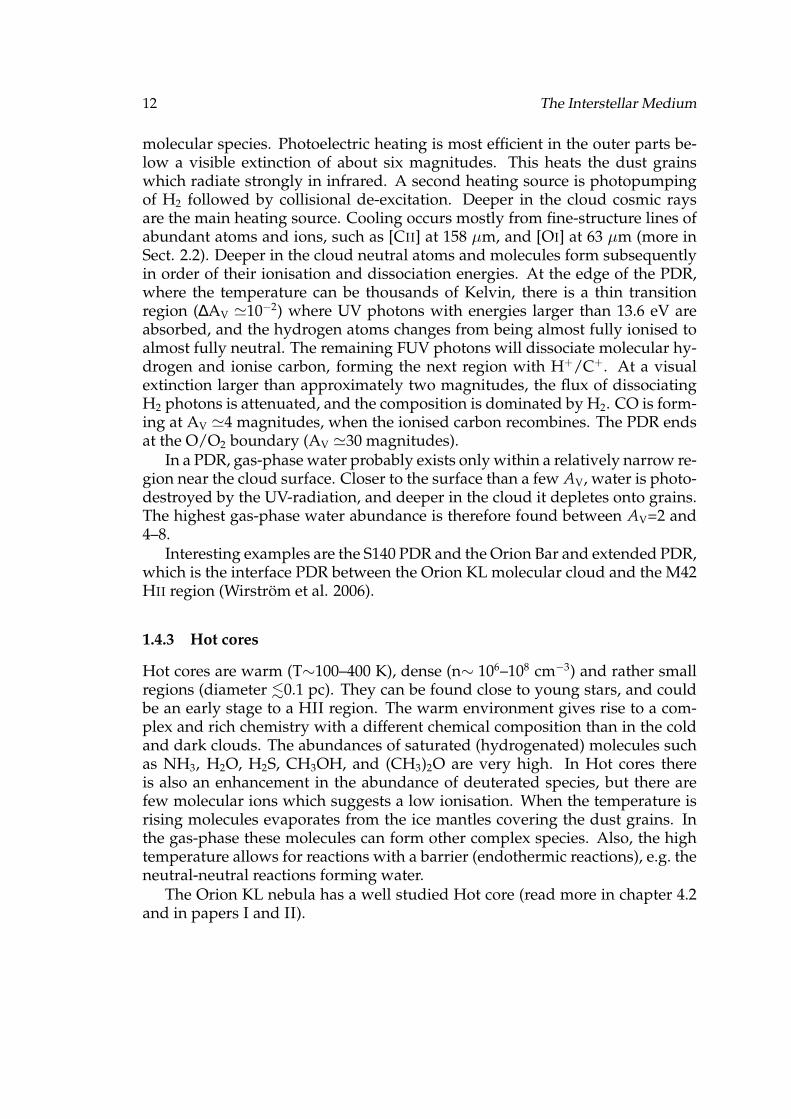
12 The Interstellar Medium
molecular species. Photoelectric heating is most efficient in the outer parts be-low a visible extinction of about six magnitudes. This heats the dust grainswhich radiate strongly in infrared. A second heating source is photopumpingof H2 followed by collisional de-excitation. Deeper in the cloud cosmic raysare the main heating source. Cooling occurs mostly from fine-structure lines ofabundant atoms and ions, such as [CII] at 158 µm, and [OI] at 63 µm (more inSect. 2.2). Deeper in the cloud neutral atoms and molecules form subsequentlyin order of their ionisation and dissociation energies. At the edge of the PDR,where the temperature can be thousands of Kelvin, there is a thin transitionregion (∆AV '10−2) where UV photons with energies larger than 13.6 eV areabsorbed, and the hydrogen atoms changes from being almost fully ionised toalmost fully neutral. The remaining FUV photons will dissociate molecular hy-drogen and ionise carbon, forming the next region with H+/C+. At a visualextinction larger than approximately two magnitudes, the flux of dissociatingH2 photons is attenuated, and the composition is dominated by H2. CO is form-ing at AV '4 magnitudes, when the ionised carbon recombines. The PDR endsat the O/O2 boundary (AV '30 magnitudes).
In a PDR, gas-phase water probably exists only within a relatively narrow re-gion near the cloud surface. Closer to the surface than a few AV, water is photo-destroyed by the UV-radiation, and deeper in the cloud it depletes onto grains.The highest gas-phase water abundance is therefore found between AV=2 and4–8.
Interesting examples are the S140 PDR and the Orion Bar and extended PDR,which is the interface PDR between the Orion KL molecular cloud and the M42HII region (Wirstrom et al. 2006).
1.4.3 Hot cores
Hot cores are warm (T∼100–400 K), dense (n∼ 106–108 cm−3) and rather smallregions (diameter .0.1 pc). They can be found close to young stars, and couldbe an early stage to a HII region. The warm environment gives rise to a com-plex and rich chemistry with a different chemical composition than in the coldand dark clouds. The abundances of saturated (hydrogenated) molecules suchas NH3, H2O, H2S, CH3OH, and (CH3)2O are very high. In Hot cores thereis also an enhancement in the abundance of deuterated species, but there arefew molecular ions which suggests a low ionisation. When the temperature isrising molecules evaporates from the ice mantles covering the dust grains. Inthe gas-phase these molecules can form other complex species. Also, the hightemperature allows for reactions with a barrier (endothermic reactions), e.g. theneutral-neutral reactions forming water.
The Orion KL nebula has a well studied Hot core (read more in chapter 4.2and in papers I and II).

1.4 Molecular environments 13
1.4.4 Shocks and outflows
A shock occurs whenever a disturbance through the medium has a speed greaterthan the speed of sound, which is about 1 km s−1 in a neutral gas with temper-ature below 100 K. The energy of a shock with about 30 km s−1 speed (con-tinuous C-shock), or from energetic outflows from a protostar can elevate thetemperature to thousands of K, and this changes the chemistry in the ISM. Inthe stronger J-shocks (Jump shocks) the temperature can be as high as 10 000 K.At these high temperatures, neutral-neutral reactions are very efficient, even forthose with high activation barriers.
The water molecule is rapidly produced in these conditions, converting allneutral atomic oxygen to H2O. Molecules from dust grains and even grain corematerial are released by sputtering. If the shock speed is too high (above 100km s−1), the molecules will dissociate.
The sources of shocks include the interaction of Supernova-Remnants withmolecular clouds, cloud-cloud collisions, or molecular outflows from newlyborn stars.
During the very early stages of a protostar, when it is still embedded in-side the parental could, outflows will be seen (Shang et al. 2006 and referencestherein). On large scales typically bipolar molecular outflows are seen. They of-ten have low-velocity (few tens of km s−1) and high masses (solar mass scales).This suggests that it is molecular cloud material that is swept up by powerfulwinds emerging from the new-born star.
1.4.5 Cold dark clouds
The cold (∼10 K) and dark clouds (n∼103 – 105 cm−3) have mostly molecular gaswith H2 as dominant species. Due to the high density there is no penetrationby visible or UV photons, and the ionisation is low. The chemistry is driven bycosmic rays that penetrate deep into the clouds producing the necessary ionsfor a neutral-ion driven chemistry.
Over 60 molecules have been detected in these regions (mostly with radioastronomy). Here the largest molecules are found in the form of unsaturatedcarbon chains (e.g. HC7N, HC9N, and HC11N).
The masses range from about 1 to 500 M¯, with size between ∼1–5 pc. Theseclouds can typically form one or two low-mass (.2 M¯) stars.
1.4.6 Giant Molecular Clouds (GMCs)
The majority of all stars form in these very large molecular gas clouds. Theyare able to form thousands of low-mass stars and several high-mass stars whichcannot form elsewhere. Once a GMC has formed, the star-formation starts al-most immediately.

14 The Interstellar Medium
GMC’s are the most massive individual objects in the Galaxy with massesfrom about 104–106 M¯, and a mean density from about 100 to 1 000 cm−3. Morethan half the total gas mass in the Galaxy is found in GMC’s. Their sizes areabout 50 pc, but some are elongated with an extent of 100 pc. Their lifetimes areabout 107 years. Once a bright O star is formed the destruction of the GMC willstart due to the intense emission of UV radiation which dissociates and ionisesthe molecules and atoms. Since GMC’s are typically found in the spiral armsthis implies also that the lifetime cannot be longer than the travel-time across aspiral arm, which is about 50 millions of years.
The internal pressure is about ten times higher than the pressure of the am-bient ISM. This suggests that they are self-gravitating objects, i.e. they are heldtogether by the mass of the molecular gas within them, otherwise they wouldfall apart in about 10 million years.
The internal structure is inhomogeneous with fragments in dense sheets, fil-aments, cores and large low-density voids. Clumps of higher than average den-sity gas fill ∼5–10% of the volume of the cloud, and in their very densest centralparts the most tightly gravitationally bound clumps form stars . Most of the gasin GMCs is thus inactive/sterile.
About 100 molecular species have been detected in GMCs. Examples ofGMCs or GMC complexes are the Orion Molecular Cloud, Sagittarius, and theEagle Nebula.

Chapter 2
Star-formation
2.1 Jeans mass and star-formation
The standard theory of star-formation describes the gravitational collapse of acold (10-120 K) and dense cloud core. The forces taken into account are grav-ity, and the opposing thermal pressure. A cloud of gas will collapse under theinfluence of gravitation if the mass of the cloud exceeds the Jeans mass
MJ '(
5 kB T
G µ mH
)3/2√
3
4π ρo(2.1)
Here kB is the Boltzmann constant, G is the gravitational constant, T is the localtemperature of the cloud, µ is the mean molecular weight, mH is the hydrogenmass, and ρ0 is the mean density of the cloud. This equation shows the impor-tance of low temperature and a high density, thus in the small cores inside theGMCs star-formation will most naturally occur. Eq. 2.1 also implies the impor-tance of cooling to keep the temperature and pressure low enough not to stopthe gravitational contraction (see Sect. 2.2).
The collapse starts with a free-fall phase with an almost constant temperature(iso-thermal phase), and is characterized by a free-fall time
t f f =
√
3π
32
1
G ρo(2.2)
Note that this time is independent of the initial radius of the cloud, which isassumed to be spherical. For a cloud of initial density of 10−19 g cm−3, and atemperature of 10 K, the free-fall time is around 2×10⁵ years.
The rate of mass infall near the core’s centre is given by
M ≈ a3
G∼ T2/3
G(2.3)
15

16 Star-formation
where a is the sound speed which is proportional to the square root of the tem-perature. The equality holds to within an order of a magnitude. Thus the pre-dicted infall mass rate does not depend on the initial cloud density, but only onthe temperature. Since a cloud of a fixed mass with higher density has a shorterfree-fall time (Eq. 2.2), the accreted mass will be smaller.
This gravitational collapse scenario explain the formation of stars, but theactual details of the event depend on the physical conditions in the star-formingregions. This also determines the mass of the resulting star, and if a double staror a planetary system will be formed. From observations we know that starshave masses between 0.08 to ∼100 M¯, where most of the stars are small, andabout half of all stars are double star systems. The star-formation rate per unitmass varies a lot within our Galaxy, but in total is ∼2-3 M¯ year−1.
However, if the Galaxy contains about 109 M¯ molecular gas, and most ofthe gas is residing in GMC’s which are gravitationally unstable, this shouldproduce a star-formation rate higher than about 200 M¯ each year. Since theobservations shows about a hundred times lower rate, this suggests that anadditional force is counteracting the gravitational collapse.
This force is caused by the magnetic fields which permeate and give supportto the clouds. In order for gravitational collapse to start, the gas cloud mustfirst lose its magnetic support. This is done with ambipolar diffusion which isthe drift of neutral relative charged particles. The magnetic field is only actingon the charged particles, while the neutral particles that carry most of the massare affected by the inward gravitational force. If the ionisation is high, the timefor the neutral species to drift inwards through the ion gas will be longer thanin the case of low ionisation. The effectiveness of a cloud collapse is thereforegoverned by the fractional ionisation in the cloud, which in turn is controlledmainly by cosmic rays deep into clouds.
The actual onset of a collapse could be triggered by collisions between cloudsstreaming across a spiral arm, leading to compression to higher densities.
2.2 Heating and cooling
As governed by thermodynamics, the temperature inside a collapsing cloudwill rise. For a rapid collapse to occur, this thermal pressure support must bekept low by cooling. As long as the cloud is optically thin and has effectivecoolants which can radiate away the gravitational potential energy that is re-leased during the collapse, the temperature can be kept almost constant and thecollapse will be prompt. However, if no coolants are available or are inefficient,the cloud will be heated according to Eq. 2.1, which leads to a higher Jeans massand the collapse will stop.
Heating and cooling occur by a variety of processes, with radiation as the

2.2 Heating and cooling 17
dominant transport mechanism. If matter is exposed to a radiation field it canextract energy and is heated (see Appendix A). When a high-energy photonionises an atom or molecule, the kinetic energy of the electron will be the dif-ference of the photon energy and the ionisation energy. The electron will sharethis kinetic energy with other gas particles through collisions, and thus the gaswill become hotter. Cosmic rays are another heating source, which can reachdeep into dense and dark clouds where radiation is blocked by molecules anddust particles.
Cooling occurs when ionisation or excitation in an atom or molecule is causedby a collision, and is de-excited by a radiative transition before another collisionoccurs (see Appendix A). The kinetic energy in the gas is then transferred to ra-diation that escapes the cloud, which therefore is cooling. Atomic hydrogen isvery effective in cooling gas to temperatures around 10 000 K. At lower temper-atures there are too few collisions that are able to ionise or excite the hydrogenatoms and the cooling stops.
To be an efficient coolant a species must have a high abundance and haveexcitation levels comparable to the average kinetic energy in the cloud. This iswhy molecular clouds are colder than atomic gas. Molecules have more avail-able very low energy levels as compared to atomic transitions. Well-knownmolecular gas coolants are CO, C, H2O, OH, and H2, with CO as the most im-portant coolant at low densities. The first excited rotational level of p-H2 hasan upper state energy of 510 K, OH has Eu = 120 K, o-H2O has Eu = 27 K, C hasEu = 24 K, while the lowest level in CO is only 5.5 K above the ground state.In addition CO has closely spaced rotational levels, is easily excited, and is thesecond most abundant molecule after H2. Thus cooling by CO produces verylow gas temperatures in molecular clouds. At a density of n(H2) = 103 cm−3, theisotopologue 13CO starts contributing to the cooling. Despite the much lowerabundance (about 40-70 times lower than 12CO), the 13CO and 12CO cooling canbe of the same order, because the latter is optically thick and the emitted pho-tons are re-absorbed. Water becomes increasingly more important as a coolantwith higher density and temperature, due to the high dipole moment. At tem-peratures above 300 K, water is the dominant coolant. At high temperatures andlow densities, H2 is the dominant coolant, while generally unimportant below100 K.
Other criteria for efficient cooling agents are a high probability for excitationduring the collision. The Einstein A-coefficient should be large to guaranteea decay occurring before a second collision. The cloud also need to be opti-cally thin at the frequency of the emitted photon – otherwise the photon will betrapped and re-absorbed within the cloud.
For diffuse clouds with higher temperatures and PDR’s, the most importantcoolants are fine-structure transitions of [CII] at 158 µm (Eu = 92 K), [OI] at 63µm (Eu = 228K), and [SiII] at 35 µm (Eu = 414 K).

18 Star-formation
2.3 The first stars
The gas in the Early Universe mainly consisted of neutral hydrogen and he-lium, with trace amounts of deuterium and lithium. Efficient molecular hydro-gen production needs the surface of dust grains since two colliding hydrogenatoms cannot associate directly. But in the Early Universe no dust grains wereavailable for molecular production. Instead it was the small ionised fractionof the gas, that gave two important, but rather inefficient and indirect ways toform H2. The first one uses an electron as a catalyst. In the first step the electronattaches itself to an H atom to form the negative ion H− (radiative association).When this ion collides with an H atom the electron will carry away energy andH2 will form. The second route involved protons instead of electrons in thesame way. A proton and a H atom radiatively associate to form H+
2 by chargetransfer. Another collision with an H atom will produce H2, while the energywill be carried away by the proton. The formation by electrons as catalysts ismore efficient than by protons, but still none of the two processes is very ef-ficient. Furthermore, the produced H2 was easily destroyed by radiation andenergetic collisions with hydrogen atoms. The resulting H2 density was aboutone or two molecules per million of H atoms. Even so, this low abundance wasvery important. And since there was deuterium present in the primordial gas,HD was also produced with an abundance of about one molecule of HD to 105
of H2. HD is found to be the main cooling agent at temperatures around 200 K.The presence of these molecules was crucial for the necessary cooling dur-
ing the star-formation process, and made cooling to temperatures around 100K possible. But still only a few species with very low abundances were presentand the collapsing clouds were inefficiently cooled. As a consequence, the firstgeneration of stars, called Population III stars, were very massive and hencevery short-lived. But these stars produced the elements carbon, nitrogen, andoxygen. When these stars experienced a violent death as supernovas, theyseeded the Early Universe for the first time with trace amounts of these ele-ments. Thus, the pregalactic gas gradually became more enriched with other el-ements than hydrogen and helium, and therefore a wider variety of stars couldform, i.e. the masses of the stars could be lower because of the more efficientcooling.
The first Population III stars are believed to have formed at z=10–20 (Choud-hury & Ferrara 2006).
Chapter 3
Searches for Primordial Moleculesin the Early Universe
3.1 The beginning
Before about 13.7 billions years ago nothing existed. And then in a processcalled the Big Bang, our Universe – both the space itself and the matter withinit — was created. The beginning was extremely hot, but the Universe was, andstill is, expanding and therefore cooling. After about 225 s the temperature haddropped to about 9×10⁸ K, and the existing nucleons (protons and neutrons)could combine into helium, and trace amounts of lithium. In the Standard BigBang Nucleosynthesis model this was over approximately 3 minutes after theBig Bang, and about 75% by mass was then ionised hydrogen and 25% helium.By number: for each 1012 H atoms – 7×10¹⁰ 4He atoms was formed, 4×10⁷ Datoms (i.e. 2H), 7×10⁶ 3He atoms, and only 150 Li atoms. The temperature wasstill high at the time, and no neutral atoms could exist. Instead a plasma ofionised atoms and electrons existed in a thermal equilibrium with the photons.The temperatures of matter and radiation were the same. But due to the ex-pansion of space the radiation became less and less energetic. At a certain time(approximately 300 000 years after the Big Bang) the temperature had cooledto about 3 000 K. This is the time of recombination, and the protons could nowcombine with the electrons and produce neutral hydrogen.
When this happened the close thermal coupling between the matter andradiation (previously maintained by Compton scattering of photons and elec-trons) was lost. From this time forward the temperatures for matter and radia-tion evolved separately. Thus at the time of recombination the Universe becametransparent to the existing photons which today can be seen as the Cosmic Mi-crowave Background (CMB). The CMB radiation has been observed by sensi-tive radiometers on the two satellites COBE and WMAP, and shows the smalldensity/temperature fluctuations from the recombination epoch.
19

20 Searches for Primordial Molecules in the Early Universe
Figure 3.1: The history of our Universe; from the Big Bang, via the Dark Ages, theformation of the first stars and galaxies to today. Credit: NASA and Ann Field (STScI).
After the recombination the Universe became dark. The cosmic Dark Agesbegan and did not end until the formation of the first stars (Pop III) and galaxies.During this time the transition from the small density fluctuations left over fromthe Big Bang to the strong non-linear structure we observe today took place. Weobserve stars, and galaxies on large scale in a structured form of large filamentsbetween large voids. But still, there is no good understanding of how the firststars were produced, or how galaxies and clusters formed. We observe the CMBradiation and obtain information from the recombination epoch. And then wemodel a theoretical evolution from the recombination epoch to the structureobserved today, and try to fit the observations. Models predict that the first starswere very massive and short-lived, and appeared between 100 and 250 millionyears after the Big Bang. These stars altered the chemistry in the Universe byproducing the first heavy elements, and influenced the dynamics by heatingand ionising the surrounding gas.
One of the remaining big unanswered questions in astronomy is illustratedin Fig. 3.1:

3.2 Elements of our primordial medium 21
• Origin of structure. How did the Universe evolve from the near uniformityat the recombination to the structures of clusters, galaxies and voids thatwe observe today during the epoch of the Dark Ages?
Direct observations from the cosmic Dark Ages are most commonly believedto be impossible. But our aim in the search for the Primordial molecules is to doexactly this – from an initial idea of Dubrovich (1977) as amplified by Zel’dovich(1978) – to perform observations of resonant spectral lines from cloud structuresevolving during the cosmic Dark Ages.
3.2 Elements of our primordial medium
We start our investigation of the Dark Ages by an inventory of its constituents:
• Atoms/ions and electrons. After the time of the recombination most specieswere the neutral H, D, He and trace amounts of Li. The recombination wassequential in the order of the ionisation potentials, beginning with Li3+
and ending with Li+. Hydrogen became neutral at z∼1100, and heliumalready at z∼2500. However, the recombination was not instantaneous,and since the Universe expanded and cooled faster than recombinationwas completed, a small fraction of free elections and protons remained.For this reason, the recombination of Li+ was not completed.
• CMB photons. The existence of the Cosmic Microwave Background (CMB)radiation was first predicted by George Gamov in 1946, Alpher and Her-man in 1949. The discovery in 1965 was inadvertently made by ArnoPenzias and Robert Wilson who shared the 1978 Nobel prize in physicsfor their discovery. After many attempts with ground-based and balloon-borne observations, it became clear that the measurements needed to bedone from space above the Earth’s bright and obscuring atmosphere (theCMB spectrum peaks at 2 mm). NASA’s Cosmic Background Explorer(COBE) satellite was launched on 18 November 1989. The first result, onlynine months afterwards, was the most perfect blackbody radiation everobserved and supported the Big Bang theory. Moreover the CMB showeddensity (equivalent to temperature) fluctuations of the order of 1/100 000.At the time of recombination the temperature was about 3 000 K, while ob-served today only 2.73 K. The decrease in temperature is due to the cosmo-logical expansion of the Universe. These observations were major achieve-ments and the 2006 Nobel prize in physics is awarded to John Mather andGeorge Smoot, who were in charge of these measurements. The WilkinsonMicrowave Anisotropy Probe (WMAP) was launched in June of 2001 tocontinue to map the CMB temperature fluctuations with higher resolution,

22 Searches for Primordial Molecules in the Early Universe
sensitivity, and accuracy than COBE. In February 2003 WMAP released re-sults from the first year of flight data (Bennett et al. 2003), and the thirdyear results are available since March 2006 (Spergel et al. 2006).
Figure 3.2: Fractional abundances in the Early Universe of molecules and ions as a func-tion of redshift z. The calculations assume cosmological parameters Ω0 = 1, Ωb = 0.0367and h = 0.67. Credit: Lepp et al. 2002.
• Molecules. When the temperature in the Universe had dropped sufficientlythe production of molecules started. Even though the BB models pro-duce only three elements and a few isotopes, a surprisingly complicatedchemistry emerges. About 200 reactions contribute to the abundance of 23atomic and molecular species which might be important in the early Uni-verse. But the resulting abundances are highly uncertain due to difficultiesto compute or measure all the reaction rates in the typical conditions inthe early Universe. Also cosmological parameters affect the production ofmolecules. If a dark energy is incorporated in the models by invoking a de-caying cosmological constant the matter temperature will decrease muchfaster. This would shift molecular formation to a much earlier epoch, andthe limiting abundance of H2 would be doubled. Based on a Standard Big

3.3 Resonant scattering 23
Bang Nucleosynthesis model, Fig. 3.2 shows the evolution of the fractionalabundances of the molecules as functions of redshift z. This is one of themore recent models from Lepp et al. (2002).
Figure 3.3: Rotational-vibrational lines for LiH, arbitrary intensity scale. Credit: deBernardis 1993.
3.3 Resonant scattering
Since the densities of the elements are very low, absorption and emission pro-cesses are ineffective. The most efficient process to couple the CMB photonswith molecules, ions, and atoms is resonant scattering. In this process a photonis first absorbed and then re-emitted at the same frequency, but not in the samedirection (elastic scattering). The cross-section for this scattering is several or-ders of magnitude larger than the Thompson scattering between the CMB andelectrons.
This scattering does not alter the CMB spectrum, but it could smear out theprimordial spatial distribution of the CMB and produce secondary anisotropies.However, since the CMB is a diffuse background, scattering is not enough to

24 Searches for Primordial Molecules in the Early Universe
produce a signal – a peculiar velocity for the scattering source is also needed,i.e. a source velocity that is not from the cosmic expansion.
The optical depth for the transition depends on the product of the abundanceand the dipole moment of the considered species. Due to the frequency depen-dence of the cross-section, rotational or ro-vibrational lines will appear. Figure3.3 shows rotational-vibrational transitions for LiH with an arbitrary intensityscale (de Bernardis et al. 1993).
τi j =
∫
sourceσres,i j ni ds ∼ 3.37 · 10−19
∫
source|~d|2 νi j
∆νni ds (3.1)
where σres,i j is the cross-section for the resonant scattering, ni is the density ofthe species in state i, ν is the frequency of the transition, ∆ν is the width of theline, and d the dipole moment of the species.
The lines can be emission- or absorption-like depending on the sign of theradial peculiar velocity of the primordial cloud. The line width and intensitydepend on the dynamics of the primordial clouds which can be divided intothree different phases:
• Linear evolution. The perturbation in the primordial gas clouds follows theHubble expansion of the Universe. Within the cloud different parts willfulfil the conditions for resonant scattering for different redshifts. Hencethe line-widths will be very broad and the signal very weak, since theydepend on the extension in redshift of the perturbation, i.e. mass and red-shift. ∆ν/ν can be as high as 0.01 for a 1014 M¯perturbation at high z.
• Turn-around phase. At this moment the gravitational force in the primordialgas clouds matches exactly the Hubble flow and the cloud appears to benon-moving. All the scattered photons will contribute to the signal at thesame frequency. This will produce the narrowest and strongest signals,where the line width is due to thermal broadening (∆ν/ν ∼10−6).
• Non-linear collapse. The gravitational collapse of the primordial clouds be-gins. The line shape will depend on the ratio of the peculiar velocity andcollapse velocity.
The most favourable regimes for detections are during the turn-around phaseand the non-linear collapse.
When we observe a moving source the observed lines will be redshifted as
νobs =ν0
1 + z(3.2)
where z is the cosmological redshift, which is a measure of the distance andtime we look back in the Universe. This also implies a very low probability

3.4 Implications 25
to have more than one source along the line of sight with the same dynami-cal and molecular conditions. Hence, we are looking for spectral lines emittedfrom a well defined primordial source at a certain redshift. Increasing the band-width will improve the explored redshift range. Another advantage of a broadband width is the possibility to detect several lines of the same species, whichis needed to confirm the origin of the line.
The intensity of the lines can be approximated as
∆I
I∼ vp
cτi j (3.3)
where vp is the peculiar velocity of the moving cloud.
3.4 Implications
The detection of redshifted spectral line patterns from primordial moleculeswould tell us about:
• The existence of a protostructure at a given z.
• The chemical composition, peculiar velocity and mass of the primordialclouds via the properties of the line, thus constraining structure-formationmodels.
• The accuracy of Big Bang Nucleosynthesis models.
• The epoch of first star formation and setting constraints on the time ofreionization
The only spectral signature produced before the epoch of the first Pop IIIstars is the resonant spectral lines. Hence a serious detection attempt should beone of the main cosmological items.
3.5 Observations
3.5.1 Previous observations
The only previous observations were made with the IRAM 30 m telescope in1992 by de Bernardis et al. Seven high-latitude regions were investigated witha 1 GHz band at 3 different frequencies in the 1.3, 2 and 3 mm atmosphericwindows where two ro-vibrational bands of LiH are expected from z∼180. Nolines were seen, but upper limits (depending on the redshift of the cloud) of theorder of 20 mK for the intensity of the LiH lines were calculated.

26 Searches for Primordial Molecules in the Early Universe
3.5.2 Our Odin observations
When looking for primordial resonant lines, several things need to be consid-ered. A broad band is needed to explore a wide range of redshift, and also toenable observations of several lines from a species to check the origin of the line.Since the lines are expected to be very weak, a low noise-level is also required.
Since the abundance determinations are very uncertain, it is difficult to pre-dict what species and lines we are looking for. Ten years ago, LiH was believedto be the best candidate for a resonant line detection, due to its high dipole mo-ment and the, at the time, believed high abundance of ∼10−10 after freeze out.More recent models find an abundance of ∼10−18–10−20. In this case, a signalwill not be possible. Today, HeH+ is considered as a more interesting species,with an abundance of ∼10−14 at a redshift of ∼100, and a dipole moment of 1.78Debye. Other interesting species are H2 with an abundance of ∼10−5–10−6, H+
2
with ∼10−13, and HD with ∼10−10–10−12.Satellite observations also have the advantage of the absence of spectral line
poisoning by the terrestrial atmosphere.
Figure 3.4: Part of spectral line survey towards a WMAP hot spot.
• Already performed observations.
A Swedish-French Odin-team has performed a Spectral Scan with the Odinsatellite towards two WMAP Hot Spots (Bennett et al. 2003) during thesummer 2004 in the frequency band 547–578 GHz (31 GHz). The resolu-tion is 1 MHz. To cover this wide bandwidth 340 orbits were spent on theobservations.
Fig. 3.4 shows part of the 31 GHz spectral scan with a resolution of 1 MHz(0.5 km s−1). As seen the rms noise level is ∼65 mK, which was reachedby an integration time of each LO setting (i.e. 5 orbits for each setting) of

3.5 Observations 27
∼3000 s. No lines are detected, but the resulting data set is not yet fullyanalysed.
Since we do not know the exact width of the resonant lines, the resolutioncan be increased in steps, gaining a lower noise level.
• Planned observations
The distortions in the CMB background are not only spectral in characterbut also spatial. The angular size of a primordial cloud at turn-around orduring the non-linear collapse can range from arcseconds to many arcmin-utes. Since the size of the clouds or their redshifts are not known, we havean observational problem. The resulting spectrum from the observationsis the difference between an on- and an off-position. If the off-position istoo close to an emitting source, a possible signal would disappear.
Figure 3.5: Observing strategy for Primordial molecule observations during winter06/07 with the Odin satellite.
We have therefore developed a new observing strategy for the upcomingOdin observations illustrated in Fig. 3.5. We have been awarded time fornew observations with the Odin satellite – 10 full weekends, which meansabout 430 orbits in total. We will perform a spectral line survey in the fre-quency ranges 542.0-547.5 GHz and 486.5-492.0 GHz towards four differ-ent points, i.e. in total 11 GHz spectral line survey for each position. Thereare a number of different redshifted lines that can fall into these frequencybands, such as the HeH+ J = 1 – 0 transition which shifts to 545 GHz atz=2.7, the J = 2 – 1 from z=6.4, and the v = 1 – 0 R(0) shifts to 545 GHz atz=162. The position of the first point is the same as used in previous ob-servations, a Hot Spot as detected by the WMAP satellite with coordinatesR.A. 05h26m00s.0, Dec. -4830’00”.0 (J2000). The positions of the second,third and fourth point are 5’, 20’ and 30’ away from the first point in dec-lination. We will have four times more integration time for every settingin this spectral line survey as compared to our previous observations, tolower the noise. In addition we will have six different spacings with obser-vations of only four positions as seen in Fig. 3.5. This will allow us to test

28 Searches for Primordial Molecules in the Early Universe
six different combinations of positions and hence sizes of the primordialclouds.
3.6 Future prospects
Our next future step will be to use ESA’s Herschel Space Observatory1, whichis much more sensitive than Odin and also allows coverage of a very large fre-quency range.
However, what we really would need is a dedicated space mission for thiskey cosmology project!
1http://sci.esa.int/science-e/www/area/index.cfm?fareaid=16

Chapter 4
Introduction to Paper I and Paper II
4.1 The Odin satellite
The accurate determination of the water and oxygen abundances in the variousphases of the ISM poses a severe observational difficulty. Due to the absorp-tion by water and oxygen, the terrestrial atmosphere is completely opaque atfrequencies around 119, 487 and 557 GHz. Any observations in these spec-tral regions have to be done from space or balloon experiments. The Odinsub-millimetre wave spectroscopy satellite is especially designed to solve theseproblems. And despite the use of advanced technology and the combinationof two scientific disciplines on a single satellite – astronomy and aeronomy –Odin is a small, low-cost, and successful spacecraft. The astronomical scientificobjectives are to study the water and oxygen chemistry in the ISM and star-formation regions, comets and circumstellar envelopes, while the aeronomersstudy molecules relevant to ozone depletion. Additional lines from species likeammonia, and carbon monoxide with isotopologues are also observable andcan aid the analysis of water and oxygen, .
The Odin satellite was launched on 20 February 2001 by a Start-1 rocket fromSvobodny in far-eastern Russia. The orbit is sun-synchronous at an altitudeof about 600 km. Odin has successfully been operating for almost six yearswhile the promised life-time was only two years. Nordh et al. (2003) and thesubsequent papers in the A&A ”Special Letters Edition: First Science with theODIN satellite” describe the satellite and its first science in detail. More recentprogress is discussed by Hjalmarson et al. (2005).
The Odin satellite is a next sensitive step after the SWAS satellite which hada 3’.3×4’.5 beam size, and non-tunable receivers (Melnick et al. 2000 and sub-sequent ApJ papers in that issue). Odin is equipped with an offset Gregoriantelescope of diameter 1.1 m, with beam widths of 2’.1 and 10’.0 at 557 GHz and119 GHz, respectively. The receiver package is actively cooled to about 140 Kand consists of four tunable sub-mm Schottky mixers. The frequency bands
29

30 Introduction to Paper I and Paper II
covered are 486–504 GHz and 541–581 GHz. In addition a fixed-tuned HEMTreceiver at 118.750 GHz for sensitive O2 searches was added in the later phase ofthe extended instrument planning. Any combination of three receivers can besimultaneously used together with a broadband acousto-optical spectrometer(AOS): BW=1 050 MHz, resolution 0.6 MHz, and two flexible hybrid autocor-relation spectrometers (AC1 and AC2): BW=100–800 MHz, resolution 0.125–1MHz. The main beam antenna efficiency is close to 0.9 which makes the inten-sity calibration very accurate.
The tunable receivers enable Odin to perform a full spectral line survey in aspectral region previously unobserved, as described in Sect. 4.3 and in Paper Iand Paper II.
The Odin satellite addresses several key-questions to be even more accu-rately addressed by ESA’s up-coming Herschel satellite (launch planned early2008). It will be located at the second Lagrange point (L2) of the Earth-Sun sys-tem, and will cover the full far infrared and sub-millimetre wave-band (60–670µm) with an order of a magnitude more sensitive SIS mixers and a 3.5 m mirror– the largest civilian mirror ever deployed in space. The Odin science can there-fore serve in important pilot studies, as e.g. our current searches for PrimordialMolecules and the Odin spectral scan survey of Orion KL.
4.2 The Orion nebula
At a distance of only ∼450 pc, the Orion KL (Kleinmann-Low) region is theclosest and most interesting high mass star-forming region, where O and B star-formation is on-going (see Genzel & Stutzki 1989 and references therein for areview). This source is very complex and chemically structured and containsextremely young and massive embedded stars which are not yet visible due tothe surrounding dust. It is the brightest infrared region in the 1 large OrionMolecular Cloud OMC-1 complex, situated about 1’ NW behind the Trapeziumstars in the sword of the Orion constellation. The Trapezium is one of the mostfamous high-mass star-forming regions. The brightest object is Θ1 C Ori, withspectral type O6 and a mass of 33 M¯. These stars are situated close to thecentre of a dense cluster, where the stellar density near the centre is about 10 000stars per pc3. About half of the cluster members are optically visible, which ispossibly to due to the UV-radiating O stars that have cleared away much ofthe ambient gas. Their intense radiation has ionised the surrounding gas in theM42 HII region in front of OMC-1. The interface between M42 and OMC-1constitutes one of the famous PDR regions in Orion (Wirstrom et al. 2003).
The chemical richness in such a star-forming region and its proximity, makesOrion KL an ideal target for spectral line surveys at millimetre and sub-mmwavelengths. And indeed, this is one of the best studied regions of the inter-

4.2 The Orion nebula 31
Figure 4.1: The Odin beam overlaid on a colour composite image of the central partof the Orion Nebula, M42, also showing the BN/KL region, based on 81 images ob-tained with the infrared multi-mode ISAAC instrument on the ESO Very Large Tele-scope (VLT) at the Paranal Observatory (ESO PR photo 03a/01 2001). The red emissionat 2 µm comes from shock excited H2 caused by a strong bipolar outflow wind from avery young massive star newly born. This is adressed in considerable detail in paper II.

32 Introduction to Paper I and Paper II
Table 4.1: Angular scales of the Orion nebula at a distance of 450 pc, as compared toangular resolution of different telescopes.
Angular scale of OrionInner solar nebula Outer solar nebula Presolar nebula Cloud core Cloud5 AU 100 AU 1000 AU 0.05 pc 0.5 pc
0”.01 0”.2 2” 23” 4’
Angular resolution at frequenciesTelescope 115 GHz 230 GHz 345 GHz 810 GHz
ALMA a 0.05”–4” 0.02”–2” 0.02”–1.5” 0.007”–0.6”
OVROb, BIMAc, IRAMd 4–7” 1–2” – –
30 m IRAMd 22” 12” 7” –
15 m JCMTe/SESTf 44” 20” 15” 6”10 m CSOg – 30” 20” 9”
3.5 m Herschelh – – 13”–45” at 1600–480 GHz1 m Odini 126” at 557 GHz
aThe Atacama Large Millimeter Array (ALMA). bOwens Valley Radio Observa-tory. cBerkeley-Illinois-Maryland Array. dInstitute de Radio Astronomie Mil-limetrique. eJames Clerk Maxwell Telescope. fSwedish-ESO Submillimetre Tele-scope. gCaltech Submillimeter Observatory. hThe Herschel Space Observatory;the largest ever IR space observatory when it is launched in 2007. iThe Odin sub-millimetre satellite (Sect. 4.1).
action of young massive stars and their parental molecular cloud. Fig. 4.1 showsa colour composite image of the Orion Nebula. The Odin beam is drawn aroundthe central position of our observations, which is the position of the most lumi-nous infrared object in the region Orion KL region, IRc2.
In addition to the chemical structure, the Orion KL region also has a com-plicated velocity field. In summary the large Odin beam (2.1 arcminutes at 557GHz) encompasses the following subsources: the bipolar Low- and High-Velocityoutflows, the Hot Core, the Compact Ridge and Extended Ridge, and the extendedPDR region. They all have different sizes, are situated at different LSR veloci-ties, and have different velocity fields. This will yield lines with characteristicline widths at characteristic LSR velocities from each subregion, which enablesan interpretation of the origin of the transitions. In addition, comparison can bemade with interferometric data for the small subsources.
But – analysis of a spectral line is not always straightforward. For examplethe emission from a single molecule is not restricted to one single subregion inOrion KL, but may be the result of a complicated blend from several regionsand this leads to complicated line profiles. Thus, when we attempt to derive

4.3 Summary of Paper I and Paper II 33
column densities and abundances, we have to separate the overall emissioninto its constituent parts.
Observations have different spatial resolutions (as well as spectral ones) de-pending on the size of the telescope. This determines what emission will fallinto our beam. When observing with a high resolution telescope, or by inter-ferometry, we see emission only from small scales. Everything larger than thebeam will not be seen. So a combination of observations with high and low spa-tial resolution is required to perform a complete description of the region ofinterest. The scale of the studied objects in the Orion Nebula, is illustrated inTable 4.1, both in physical length (pc) and angular scales, along with the spa-tial resolution of several well known telescopes. As is clearly seen, the requiredhigh resolution to observe the smallest inner parts will not be available until theALMA interferometer is in operation on the high-altitude Llano de Chajnantor(5000 m elevation) in the Chilean Andes1. Each of ALMA’s movable antennadishes will measure 12 m wide. The array will measure 150 m to 14 km, and willcover a frequency range from 30 to 950 GHz. The construction of ALMA startedin 2003, will become incrementally operational from 2010 on, and is planned tobe completed in 2012,
4.3 Summary of Paper I and Paper II
A spectral line survey is an ideal opportunity for an unbiased search of newspecies, and to establish which molecules are present and their abundances inthe observed gas. The derived abundances and temperatures are then usedto constrain chemical models of molecular production in regions with varyingtemperature, density and physical conditions such as shocks or outflows.
Many ground-based spectral line surveys have been made of the Orion KLregion, at both lower and higher frequencies, but due to the absorption by wa-ter and oxygen, the terrestrial atmosphere is completely opaque at frequenciesaround 487 and 557 GHz. To cover these frequencies we have used the Odinsatellite to perform a spectral line survey in the frequency ranges 486–492 GHzand 541–577 GHz, not possible to observe from ground, filling the gaps betweenprevious spectral scans.
After extensive data-reduction work, a long spectrum of total 42 GHz wasobtained. The next step was then to decide what features should be called lines– or only noise. When this was done, all the 347 lines needed identifications –if possible. The most important aspect of line identification is to have accuratefrequencies of the transitions. We have used several databases for this purpose,such as the SLAIM∅3 molecular line catalogue2 available on CD (Lovas 2003),
1http://www.eso.org/projects/alma/2Not available on-line, but some of its content is found at http://physics.nist.gov/PhysRefData/

34 Introduction to Paper I and Paper II
the Cologne Database for Molecular Spectroscopy3 (CDMS, Muller et al. 2001)and the Jet Propulsion Laboratory4 database (JPL, Pickett et al. 1998) and theLeiden5 database (Schoier et al. 2005). In these databases frequencies of tran-sitions in these spectral regions can be found, as well as other molecular pa-rameters (upper state energy, transition quantum numbers, A-coefficient or linestrength). Unfortunately, these databases are not complete. The spectroscopystill is sparse at higher frequencies and a number of unidentified lines in oursurvey are likely to be poorly known transitions of the identified molecules andtheir isotopologues, including their vibrationally or torsionally excited states.
Line identification is not only finding a frequency of a transition that matchesthe observed feature. Very often, many transitions lie well within the observedline width and are therefore possible candidates of origin. But the chemistryand abundance of a species can suggest an origin of the lines, and as a start-ing point previously observed species can be considered. The line shape andstrength have to be taken into account as well as the presence of other expectedline features from the same species. As a first approximation an LTE modelis assumed thereby giving the integrated intensities of the transitions from thevarious upper states.
Some of the results from the Orion KL spectral line survey:
1. We have detected 38 different molecular species with a total of 347 lines.
2. The unidentified lines are 19% of the total. Some tentative assignmentsof a few of them have been made such as the first interstellar anion, SH−,SO+, ND and CH3OCHO.
3. The total emission in our survey is dominated by CO, o-H2O, SO2, SO,13CO and CH3OH. Species with the largest number of lines are CH3OH,(CH3)2O, SO2, 13CH3OH, CH3CN and NO.
4. Six water lines are detected including the ground state transition 11,0 – 10,1
of o-H2O, and isotopologues o-H182 O and o-H17
2 O. A weak line feature at489.054 GHz is identified as the 42,3 – 33,0 transition of o-H18
2 O with an up-per state energy of 430 K. Hot Core emission from water is observed fromthe p-H2O transition 62,4 – 71,7 with upper state energy 867 K. We have alsoobserved the HDO 20,2 – 11,1 transition from the Low Velocity Flow andCompact Ridge, and have a tentative detection of the high energy transi-tion (581 K) 62,4 – 62,5 of HDO.
5. The 10 – 00 transitions of NH3 and the isotopologue 15NH3 are observed.
3http://www.ph1.uni-koeln.de/vorhersagen/4http://spec.jpl.nasa.gov/5http://www.strw.leidenuniv.nl/∼moldata/

4.3 Summary of Paper I and Paper II 35
6. Abundance ratios of [D/H], [12C/13C], [32S/34S], [34S/33S], [18O/17O], and[O/S] are calculated.
7. Different methods are used to obtain rotation temperatures and columndensities. For 8 different species which had at least four lines and a suffi-cient energy range in the transitions, the rotation diagram method is ap-plied. The other methods used as comparison models are the LTE approx-imation for a single line, and the forward model.
8. Abundances are estimated for the observed species from the different sub-regions, and we find very high gas-phase abundances of H2O, NH3, SO2,SO, NO, and CH3OH.
9. The number of lines is 4 – 20 per GHz, with a mean of 8 per GHz. Thisis comparable with larger telescopes (∼10 GHz−1), showing the excellentperformance of the Odin satellite.
10. The apparent noise level is higher than expected from the integration time,which suggets that we are approaching a line forest of unidentified lines(the ”confusion limit”).
11. A lower limit to the line-to-continuum ratio is 0.2, which is consistent withprevious estimations.

36 Introduction to Paper I and Paper II

Paper I
A spectral line survey of Orion KL from 486 – 492 and541 – 577 GHz with the Odin satellite.
I. The Data
To be submitted to Astronomy & Astrophysics
37

38 Introduction to Paper I and Paper II

Paper II
A spectral line survey of Orion KL from 486 – 492 and541 – 577 GHz with the Odin satellite.
II. Data analysis
To be submitted to Astronomy & Astrophysics
61

62 Introduction to Paper I and Paper II

Abstract of poster
Progress in searches for primordial resonant lines usingthe Odin satellite
IAU Symposium 231, Astrochemistry: Recent Successes and Current Challenges231, 241, 2005
109

110 Introduction to Paper I and Paper II

Appendix A
Tools of astronomy
A.1 Radiative transfer
With the equation of radiative transfer we describe how the intensity changeswhen the radiation travels from a source through a medium towards us. Pho-tons can be added to the original beam of radiation from the medium it travelsthrough. They can also be removed by scattering or absorption. If no local emis-sion or extinction occurs, the intensity stay constant along the way.
To describe the amount of intensity added by local photon emission to thebeam, we use the frequency-dependent emission coefficient jν , which is definedas:
jν ≡dEν
dV dt dν dΩ=
d Iν(s)
ds. (A.1)
This expression describes the energy dEν that is added in the form of photonsto a beam with solid angle dΩ, over the bandwidth dν, during a time dt, withinthe volume dV. This is the same as the change of intensity along the travelledpath ds. The dimensions of jν are [erg cm−3 s−1 Hz−1 sr−1].
The removal of emission from the beam is proportional to the number ofextinguishing particles and to the supply of photons. The frequency-dependentproportionality constant is called the extinction coefficient, and can be definedper particle, per gram, or per cm2.
d Iν ≡ −σν n Iν d s ≡ κν ρ Iν ds ≡ −αν Iν ds. (A.2)
where n is the density of the absorbing particles [cm−3], σν is the effective cross-section per particle [cm2], and κν is the monochromatic mass extinction coeffi-cient (the opacity, [cm2 g−1]), and ρ is the mass density [g cm−3], and αν is themonochromatic linear extinction coefficient [cm−1]. In this section the transportof radiation is described with the extinction per cm, αν .
Using the emission- and absorption coefficients the change of intensity as it
113

114 Tools of astronomy
travels through a medium can be written as:
d Iνds
= jν − αν Iν . (A.3)
This is the equation of radiative transfer, and can be used generally exceptwhen the absorbing particles are large with respect to their mean distance, or ifthey are not randomly distributed in the medium.
A.1.1 Optical depth and source function
To further simplify Eq. (A.3) we use the optical depth concept:
dτν(s′) ≡ −αν ds′ (A.4)
The total optical depth is obtained by integrating (A.4) over the total path, s,travelled from the source to us.
τν = −∫ s
0αν ds′ =
∫ 0
sαν ds′. (A.5)
The optical depth is thus integrated against the direction of travel with τν=0 atthe observer and τν = ∞ at an infinite distance. It measures the photon-escapefrom a medium, and therefore describes the radiation as we see it.
The opacity can also be viewed upon as the inverse of the average distancetravelled between collisions, or the mean free path, l, which is
l =υ t
n σν υ t=
1
n σν=
1
αν. (A.6)
The number of mean free paths, as measured along the ray’s path is therefore anotherexpression for the optical depth. If the extinction is high a photon will travel onlya very short distance before it collides, and therefore it will be trapped withinthe medium. The radiation cannot escape the medium unless the optical depthis about one or less. Note, that the mean free path and the optical depth aredifferent for photons of different frequencies.
The ratio of emission- and absorption coefficient is called the source function
Sν ≡jναν
. (A.7)
The source function depends only on the local temperature of the cloud.The dimensions are the same as for the intensity, and these two quantities canbe added or subtracted. The source function specifies the addition of photonsalong the path of the beam.

A.1 Radiative transfer 115
We can now rewrite Eq. (A.3) as
− dIναν ds
= Iν −jναν
(A.8)
dIνdτν
= Iν − Sν . (A.9)
A.1.2 Solution of the transport equation
For pure extinction jν = 0, and the transport equation will be reduced to
dIνdτν
= Iν , (A.10)
which has the solution
Iν = Iν,0 e−τν . (A.11)
The infalling intensity decreases exponentially by the optical depth along theray.
The limit between small and large extinction is found at 1/e, and τν = 1. Thegas is called optically thick if τν > 1 and optically thin if τν < 1. An opticallythin medium is one in which a photon can traverse the medium without beingabsorbed, whereas in an optically thick medium the photon will be absorbed.
In addition to extinction there is also emission
dIν = jν ds = Sν dτν (A.12)
which must be added to the equation. This emission must be multiplied by adiminishing exponential to correct for the absorption from the emitting cloud.
With both these contributions the solution of the transport equation will be:
Iν(τν) = Iν,0 e−τν +
∫ τν
0Sν(τ ′
ν) e−(τν−τ ′ν ) dτ ′
ν . (A.13)
If we assume that the cloud is homogeneous and the source function Sν is con-stant, the solution will be simple:
Iν(τν) = Iν,0 e−τν + Sν(1 − e−τν ). (A.14)
Here, the first term represents the damping of the infalling intensity whenthe radiation passes through the cloud. The second term is the emission con-tribution from the cloud, corrected for absorption when it travels through thecloud. The resulting frequency dependent intensity is thus depending on theproperties of the medium it travels through, such as the absorption coefficientsand the density of the gas-particles, and also of the temperature.

116 Tools of astronomy
Figure A.1: Special cases in (a) the optically thick limit, (b) the extreme optically thinlimit, and (c) the optically thin limit. Credit: Kaj Silander
A.1.3 Special cases
There are three special cases which have ever more simple solutions than shownby Eq. (A.14), which occur in the optically thin and thick limits.
• Optically thick limit, |τ | >> 1.
If the gas is very dense and opaque then the optical depth will be verylarge and we will have
Iν ≈ Sν . (A.15)
When we observe an optically thick medium we will obtain informationabout the emission from the surface of the cloud, as shown in Fig. A.1(a).The radiation can escape from the medium at a mean optical depth ofapproximately one and therefore an optically thick medium effectivelyblocks all infalling radiation as well as radiation from within the medium.The emergent intensity is only depending on the local temperature, andtherefore observation of optically thick emission gives direct temperatureinformation.

A.1 Radiative transfer 117
• Optically thin limit |τ | < 1.
In the less extreme thin limit, but still with little intervening gas absorbingthe intensity, the optical depth will be smaller than one. The exponentialcan then be expanded with a Taylor-series, e−τν ≈ 1 − τν and we will get:
Iν(τν) ≈ Iν,0(1 − τν) + Sν τν = Iν,0 + (Sν − Iν,0)τν . (A.16)
This simplification is correct within 5% to 10% for an optical depth of 0.1and 0.2, respectively. The source-function can very often vary substantiallyover a narrow frequency band, and this will give emission lines if the dif-ference between Sν and Iν,0 is positive, or absorption lines if its negative.
If there is no infalling radiation we will have
Iν ≈ Sν τν (A.17)
Observations of optically thin emission or absorption gives informationabout the total integrated emission along the line-of-sight as illustrated inFig. A.1(c). Information about the density or column density (see Sect.A.3) can therefore be obtained.
• Optically extreme thin limit |τ | << 1.
When the density of the intervening gas is very low and the optical depthis much below one, as seen from Eq. (A.17) the emergent intensity willsimply be:
Iν(τν) ≈ Iν,0 (A.18)
There is another special case that will not be treated any further in this workand that is when the optical depth is negative:
τν << −1. (A.19)
As seen from Eq. (A.13), a negative optical depth will increase the intensityexponentially with τν . In this case we have maser amplification.

118 Tools of astronomy
A.1.4 Discrete processes – spectral line theory
Atoms and molecules have discrete energy levels as described by quantum the-ory, which means that the radiation is quantised. There are various types ofdiscrete energy levels, for example:
• Electronic states of atoms and ions. Transitions involving valence electronshave energies typically a few to hundreds of eV and the spectra are seenin visible or UV. When transitions involve inner shells the energies can be>keV and fall in the X-ray region.
• Electronic states of molecules. The energy is typically tenths to a few eV andthe spectral region is infrared through the visible to the UV.
• Vibrational states of molecules. Molecules can also vibrate, and within theelectronic states there are vibrational levels. The energy is typically a fewtenths to one eV, and emitted in sub-mm or infrared.
• Rotational states of molecules. In addition to vibrational levels, the moleculescan rotate at discrete energy levels. Within the vibrational levels there arerotational levels with very low energy differences. The emission of rota-tional lines are typically 10−4 – 10−3 eV, and the spectra are therefore seenin the radio-regimes (mm and sub-mm). Fine- and hyperfine splittings ofrotational states have even lower energies.
Figure A.2: A two-level system with transitions between the upper state u and thelower state l. The three radiative processes are described by the Einstein coefficients.
There are five processes for excitation or de-excitation between two states asillustrated in a two-level system in Fig. A.2. The energy difference between thestates is ∆E = hν. However, in any real system, there are many levels whichmay be connected by possible physical transitions.

A.1 Radiative transfer 119
The Einstein coefficients describe the probabilities for emission and absorp-tion through the various processes. The Einstein A-coefficient is the transitionprobability for a spontaneous de-excitation per second per particle in the upperstate u [s−1]. This is only depending on atomic or molecular parameters and noton the environment, and can be calculated as:
Aul =16π3 ν3
ul µ2
3 ε0 h c3
Sul
gu, (A.20)
where µ is the molecular dipole moment which is measured in laboratories,and gu is the statistical weight of the upper level. This is the number of stateswith the same energy. For linear molecules gu=2J+1, where J is the rotationalquantum number. Sul is the intrinsic line strength and the calculations dependon the symmetry of the molecule. The line strength and dipole moment canbe found in different databases (see Sect. 4.3) or in the literature. The averagelifetime in a state u is 1/∑i Aul, where the summation of Aul is over all lowerstates l.
The next process is the radiative excitation which is described by the EinsteinBlu coefficient together with the frequency- and angle averaged intensity Iν0
.Blu Iν0
describes the number of radiative excitations per second per particle instate l.
The Einstein coefficient for stimulated emission is the de-excitation per sec-ond per particle in state u, described by Bul Iν0
. The de-excitation is stimulatedby a photon with the same energy as the difference between the upper andlower state, and the result is two photons with the same energy, in the samedirection. Blu and Bul have dimensions of [W−1 m2 Hz s].
The last two processes are collisional excitation and collisional de-excitation. TheClu and Cul coefficients describes the number of collisional excitations, or de-excitations, per second per particle in state u or l, respectively [cm−3s−1]. Thecoefficients depend on the velocities between the colliding particles, on the den-sity, and on the nature of the interaction. Collision partners may be electrons,H, H2 or He, with H2 as the dominant collision agent in dense molecular clouds.As an example, a transition from state i to state j from a collision between anatom an an electron is described by:
ni Ci j = ni Ne
∫ ∞
υ0
σi j(υ) f (υ)υ dυ (A.21)
with ni as the number density in state i, Ne is the electron number density, σi j
is the collisional cross section, f (υ) is the velocity distribution, and υo gives thethreshold kinetic energy by 1/2mv 2
0 .Generally, the Einstein coefficients are related to each other through
Aul =2hν3
ul
c2Bul and Bul =
gl
guBlu (A.22)

120 Tools of astronomy
(a) (b) (c) (d)
creationphotonphoton
destructionphoton
scatteringphoton
conversion
u
l
Figure A.3: An illustration of transitions between two states by different processes,which creates, destroys, scatter or converts photons. Credit: Kaj Silander
A.1.5 Photon creation, destruction, scattering and conversion
• There are different kinds of interaction between discrete energy states. If aradiative excitation is followed by a collisional de-excitation, then a photonwill be destroyed. Radiation will be transferred into kinetic energy of thegas which will heat. This is shown in Fig. A.3(a).
• If collisional excitation is followed by a radiative de-excitation (sponta-neous or induced) a photon will be created, Fig. A.3(b). When this hap-pens the kinetic energy in the colliding species will be transferred to radi-ation. By this process a gas is able to cool if the optical depth is low and thecreated photon is able to escape the cloud.
• When a radiative excitation is followed by radiative de-excitation the pho-ton will change direction and the radiation will be re-distributed, Fig.A.3(c).In elastic scattering (resonant, Rayleigh or Thomson scattering) the fre-quency is maintained, while in inelastic scattering, such as Compton orinverse Compton scattering, the frequency will be altered. In the specialcase of stimulated emission, the direction is preserved.
• In the last shown process in Fig. A.3(d), a species is radiatively excited, andthen followed by de-excitation in two (or several) steps. This will changethe energies of an energetic photon into two or mores photons with lowerfrequencies and thus with lower energies. By this the gas is able to cool ifthe cloud is optically thin for the created photons.
In the first two processes, the local kinetic energy of the gas particles andthe radiation energy in the photons are transformed into one another. If these

A.1 Radiative transfer 121
processes are frequent, there will be strong coupling between the local radiationfield and the local particle velocities, which is the same as the kinetic tempera-ture of the gas. Thus, there will be equipartition of energy and thermodynamicequilibrium (TE) or Local TE applies (see Sect.A.1.6). However, if these pro-cesses are rare the temperatures of the radiation field and the gas may not bethe same (Non-LTE case). In this case the photon might have been scatteredseveral times after its creation. Thus, the radiation we see might not tell theobserver anything about the conditions from where the photons are emitted.
A.1.6 Types of equilibrium
• Thermodynamic Al equilibrium (TE).
This occurs in a very optically thick medium. For every subprocess de-tailed balance holds. This means that Iν = Sν = Bν , where Bν is the Planckfunction which describes the emission from a black-body
Bν =2hν3
c2
1
ehν/kT − 1(A.23)
where h is the Planck constant, c is the speed of light, and k is the Boltz-mann constant. In TE the flux of emission is zero and no emission or ab-sorption lines appear, only a thermal continuous emission as described bythe Planck function.
The population of each level in TE is described by the Boltzmann equation,which is the number density in the upper state compared to that in thelower state. This also defines the excitation temperature Tex
nu
nl
=gu
gl
e−hν/kTex (A.24)
where gu and gl are the statistical weights of the upper and lower states,and hν=Eu-El.
To compare the number density in state u with the total, we may write
nu
ntot=
gu
Q(T)e−hν/kTex (A.25)
where Q(T) is the partition function and is the sum of all statistical weights,gi, from all possible states:
Q(T) =
∞∑i=0
gi e−Ei/kTex (A.26)
The partition function depends on the excitation temperature but also onmolecular constants and will therefore be different for different molecules.

122 Tools of astronomy
The principle of detailed balance also holds for the collisions, which leadsto a definition of the kinetic temperature TK
Clu
Cul
nu
nl
=gu
gl
e−hν/kTK (A.27)
This relation holds generally, even outside TE.
When collisions dominate there will be strong coupling between the lo-cal radiation field and the local particle velocities. Thus, the temperatureof the gas and radiation is in equilibrium and is the same, the gas is ther-malised and Trad=TK=Tex.
• Local thermodynamic equilibrium (LTE)
The mean free path of the particles is smaller than the scale of tempera-ture variations, therefore the matter will experience a local TE and will bein equilibrium with the ambient kinetic temperature. However, the radia-tion temperature might deviate from the kinetic temperature and can varyslowly through the medium, but Tex ≈ TK. Hence Sν = Bν , but Iν 6= Bν .
The Boltzmann equation still holds in LTE since the energy-distribution ofmatter is maintained locally by collisions and not by radiation.
• Statistic equilibrium (SE).
The assumption of statistical equilibrium implies that the radiation and thelevel populations are time independent and all upwards and downwardsprocesses are balanced and
Nl (Iν0Blu + n Clu) = Nu (Iν0
Bul + n Cul + Aul), (A.28)
with Iν0as the frequency- and angle-averaged intensity, n as the number
density of the collision partner, and Nl and Nu as the level populations inthe lower and upper levels, respectively.
Since the temperatures are not the same, and might also differ betweentransitions in the same species, this calculation must be performed for ev-ery pair of states.
A.1.7 Critical density
When the collisions in the gas start to dominate the downward transitions, inthe two-level system the density is able to bring Tex midway between Trad andTK. This density is referred to as the critical density. A commonly used first orderapproximation in a two level system is
ncrit =Aul
Cul
(
1 +1
e hν/kT − 1
)
≈ Aul
Cul
. (A.29)

A.2 Radioastronomy 123
The approximation holds if hν >> kT and is widely used as a first approxima-tion of ncrit. A lower limit to the density in order to produce observable emissionmay be approximated by
nmin & 1011 Aul
√TK
T0[cm−3] (A.30)
where we have used a mean velocity of the gas particles < υ >≈104√
TK [cm s−1],a cross-section approximated by the dimensions of a molecule, σ ∼10−15 cm−2,and Cul ≈ nσ < υ >. This value must be multiplied with TK/T0 for the excitationtemperature to be at half the value of the kinetic temperature.
A.2 Radioastronomy
In the radio spectral region the wavelengths are longer than in the visible andinfrared light (from sub-mm to meter). This means that hν << kT and the ex-ponent in the Planck function can be Taylor expanded to the Rayleigh-Jeans law
Bν(T) =2ν2
c2kT. (A.31)
In radioastronomy also very often a radiation temperature J(Tex) is used, andis defined as
J(Tex) =hν
k
1
e hν/kTex − 1≈ Tex, (A.32)
where the approximation is valid only if hν << kTex. For temperatures T ≈100 – 200 K, and frequencies ∼550 GHz, the radiation temperature will differfrom Tex by approximately 10 – 15%. Accordingly, J(Tex) and not Tex should beused in calculations.
The most important property of Rayleigh-Jeans law is the proportionality ofthe temperature and the radiation. This is so useful that the radiation from anextended source is measured by its brightness temperature, Tb
Tb =c2
2kν2Bν . (A.33)
This is the temperature that would result in a given radiation if put into Rayleigh-Jeans law. Calibration procedures at radio telescopes, using thermal loads, al-lows J(T) to be expressed as Tb.
If this is applied to the equation of radiative transfer, Eq. (A.14), for an ex-tended (i.e. the source fills the beam) isothermal medium we will get:
Tb = Tb(0) e−τν + Tex(1 − e−τν ). (A.34)

124 Tools of astronomy
With no background radiation and for optically thin transition (A.34) sim-plifies to
Tb = Tex τν (A.35)
In case of an optically thick transition (A.34) simplifies to
Tb = Tex (A.36)
A.3 Column densities
Two properties of the gas are especially interesting: the temperature and col-umn density which is defined as
N =
∫ s
0n ds′ (A.37)
in units of [cm−2]. If we know the geometry of the source the density can thenbe calculated.
The column density can be obtained through different methods. With ob-servations of a single line, either LTE is assumed and N can be calculated, ora statistical equilibrium model can be used. If a number of transitions are ob-served the rotation diagram method can be used, which is also described andused in Paper II. The resulting formula for the column density is found by ex-pressing the absorption coefficient in terms of the Einstein coefficients
κν =hν
4π(nl Blu − nu Bul)φ(ν) (A.38)
where the normalised line profile φ(ν) is
φ(ν) =
√4 ln 2
∆ν√
πe−4 ln 2( ν
∆ν )2
. (A.39)
The optical depth of a transition from an upper state, u, to a lower state, l,with the use of (A.25), (A.22) and (??) may be written as
dτν = κνds =hνul
4π(nl Blu − nu Bul) φν ds (A.40)
=hν
4π
(
nlgu
gl
Bul − nu Bul
)
φν ds (A.41)
=hν
4π
(
nu
nl
nlehν/kTx − nu
)
c2
2hν3Aul φν ds (A.42)
=c2
8πν2Aulnu(e hν/kTul − 1) φν ds (A.43)

A.3 Column densities 125
After integrating this along the line-of-sight we obtain
τν =c2
8πkν2ul
Aul Nu
(
e hνul/kTex − 1)
φν (A.44)
Integrating over an assumed Gaussian line profile, using the Boltzmannequation Eq. (A.25) for a relation between Nu and Ntot, and switching fromfrequencies to velocities (which is most common in radioastronomy) with thesubstitution dν = ν/c dυ we get
τmax =
√
ln 2
16π3
c3
ν3ul ∆v
Aul Ntotgu
Q(T)e−Eu/kTex (e hνul/kTex − 1) (A.45)
With the assumption of optically thin emission, neglecting the backgroundradiation, and assuming that the source fills the antenna main beam, the beamaveraged upper state column density can be obtained from Eq. (A.44)
Nu =8πkν2
ul
hc3
1
Aul
∫
Tb dv (A.46)
The total column density of each species can then be found if we assumeLTE, where all the excitation temperatures for all the energy levels are the same.The molecular population of each level is then given by the Boltzmann equationand the beam-averaged total column density becomes
N tot =8πkν2
ul
hc3
1
Aul
Q(T)
gueEu/kTex
∫
Tb dv (A.47)
assuming optically thin emission.
A.3.1 Rotational diagram
If we want to calculate the total column density of a molecule we observe an op-tically thin transition, measure the integrated intensity and use it in (A.47). Butthe excitation temperature is still an unknown quantity. If we don’t know it, wecan make an educated guess and still be able to calculate the column density. Abetter way to establish the temperature is to use the rotational diagram method.If many transitions of the same species are observed, and LTE is assumed, whichmeans that only one temperature characterises all the transitions, the excitationtemperature can be calculated.
When we have observed a number of lines having a wide range of upperstate energies, we can use the rotation diagram method. If we take the logarithmof the Boltzmann equation, Eq. (A.25), we obtain

126 Tools of astronomy
lnNu
gu= ln
Ntot
Q(T)− Eu
kTex. (A.48)
The left hand side in this equation is identical to the logarithm of Eq. (A.46)divided by the statistical weight gu. We plot this quantity as a function of theupper state energy Eu in a semi-log plot. A least squares fit to the data will thenproduce a straight line with slope −1/Trot. If we extrapolate the line to Eu = 0K, we obtain the total column density from the intersection of the y-axis, y0 and
Ntot = Q(T) e y0 . (A.49)
The importance of a correctly calculated partition function is obvious.However, the population distribution may not be characterised by a single
rotational temperature. The temperature can vary due to density, excitation gra-dients along the line-of-sight, IR flux, sub-thermal excitation etc. This methodalso require optically thin transitions. The optical depth can change the slopeof the rotation diagram and thereby affect both the rotation temperature andthe column density. Once a transition has become optically thick, the value ofNu/gu cannot increase any further. Then the derived total column density willbe too low and need an optical depth correction factor (see Paper II).

Bibliography
[1] Abel, T., Bryan, G.L., Norman, M.L., 2002, The Formation of the First Star inthe Universe, Science, vol 295, 93
[2] Bennett, C.L., Fixsen, D.J., Hinshaw, G., Mather, J.C., Moseley, S.H., et al.,1994, Morphology of the interstellar cooling lines detected by COBE, ApJ, 434, 587
[3] Bennett, C.L., Halpern, M., Hinshaw, G., Jarosik, N., Kogut, A., et al., 2003,First-Year Wilkinson Microwave Anisotropy Probe (WMAP) Observations: Prelim-inary Maps and Basic Results, ApJS, 148, 1
[4] Blake, D.F., Jenniskens, P., The Ice of Life, Scientific American, Aug 2001, 37
[5] Brack, A., 2002, Water - the Spring of Life, p 79 in Astrobiology - the Quest for theConditions of Life, Horneck, G., & Baumstark-Khan, C., (Eds.), Springer Verlag
[6] Cernicharo, J., and Crovisier, J., 2005, Water in Space: The Water World of ISO,SSRv, 119, 29
[7] Cheung, A.C., Rank, D.M., Townes, C.H., Thornton, D.D., and Welch, W.J.,1968, Detection of NH3 molecules in the interstellar medium by their microwaveemission, Phys Rev Letters, 21, 1701
[8] Cheung, A.C., Rank, D.M., Townes, C.H., Thornton, D.D., and Welch, W.J.,1969, Detection of Water in Interstellar Regions by its Microwave Radiation, Na-ture, vol 221, 626
[9] Choudhury, T.R., and Ferrara, A., 2006, Updating reionization scenarios afterrecent data, MNRAS, 371, L55
[10] de Bernardis, P., Dubrovich, V., Encrenaz, P., Maoli, R., Masi, S., et al., 1993,Search for LiH lines at high redshift, A&A, 269, 1
[11] Doty, S.D., van Dishoeck, E.F., van der Tak, F.F.S., and Boonman, A.M.S.,2002, Chemistry as a probe of the structures and evolution of massive star-formingregions, A&A, 389, 446
[12] Dubrovich, V., 1977 Molecules of cosmological origin, SvAL, 3, 128
127

128 BIBLIOGRAPHY
[13] Dubrovich, V., and Bajkova, A.T., 2003, A Difference Method of Searching forSpectral-Spatial Fluctuations of the Cosmic Microwave Background Radiation AstL,29, 567L
[14] Ehrenfreund, P. and Charnley, S.B., 2000, Organic Molecules in the InterstellarMedium, comets, and meterorites, ARA&A, 38, 427
[15] Evans II, N.J, 1999, Physical Conditions in Regions of Star Formation, ARA&A,37, 311
[16] Genzel, R., and Stutzki, J., 1989, The Orion Molecular Cloud and Star-formingregion, ARA&A, 27, 41
[17] Gibb, E.L, Whittet, D.C.B., Boogert, A.C.A., and Tielens, A.G.G.M., 2004,Interstellar Ice: The Infrared Space Observatory Legacy, ApJS, 151, 35
[18] Glover, S., 2005, The formation of the first stars in the universe, SSRv, 117, 445
[19] Goldsmith, P.F., and Langer, W.D., 1978, Molecular cooling and thermal bal-ance of dnese interstellar clouds, ApJ, 222, 881
[20] Hartquist, T.W., (Ed.), 1990, Molecular Astrophysics, Cambridge UniversityPress
[21] Hartquist, T.W., & Williams, D.A., 1995, The chemically controlled cosmos,Cambridge University Press
[22] Hartquist, T.W., & Williams, D.A., 1998, The molecular astrophysics of starsand galaxies, Oxford University Press
[23] Hasegawa, T.I., Kwok, S., Koning, N., Volk, K., Justtanont, K., et al., 2006Observations of the Circumstellar Water 110–101 and Ammonia 10–00 Lines in IRC+10216 by the Odin Satellite, ApJ, 637, 791
[24] Hashimoto, M., and Kamikawa, T., 2003, Effects of a decaying cosmologicalterm on the formation of molecules and first objects, ApJ, 598, 13
[25] Hjalmarson, A., Bergman, P., Biver, N., Florn, H.-G., Frisk, U., et al. , 2005,Recent astronomy highlights from the Odin satellite, AdSpR, 36, 1031
[26] Hollenbach, D.J., & Thronson, Jr., H.A., 1987, (Eds), Interstellar Processes,Reidel Publishing Company
[27] Kaufmann, M.J., and Neufled, D.A., 1996, Far-infrared water emission frommagnetohydrodynamic shockwaves, ApJ, 456, 611
[28] Lepp, S., Stancil, P.C., and Dalgarno A., 2002, Atomic and molecular processesin the early Universe, JPhB, 35, 57

BIBLIOGRAPHY 129
[29] Levy, E.H., & Lunine, J.I., (Eds.),1991, Protostars and Planets III, Universityof Arizona Press
[30] Lis, D.C., Blake, G.A., and Herbst, E., (Eds.), 2005, Astrochemistry: RecentSuccesses and Current Challenges, Proc. IAU Symposium 231, Cambridge Uni-versity Press
[31] Liseau, R., and the O2din Team, 2005, Odin Detection of O2, IAU SymposiumNo. 231: Recent Successes and Current Challenges, Lis, D.C., Blake, G.A., andHerbst, E., (Eds.), 301
[32] Longair, M.S., 1998, Galaxy formation, Springer Verlag
[33] Lovas, F.J., 2003, Spectral Line Atlas for Interstellar Molecules (SLAIM∅3) Ver.1,private communication and CD
[34] Mannings, V., Boss, A.P., Russell, S.S., (Eds.), 2000, Protostars and Planets IV,Tucson: University of Arizona Press
[35] Maoli, R., Melchiorri, F., and Tosti, D., 1994, Molecules in the postrecombina-tion universe and microwave background anisotropies, ApJ, 425, 372
[36] Maoli, R., Ferrucci, V., Melchiorri, F., Signore M., and Tosti, D., 1996, Molec-ular signals from priomordial clouds at high redshift, ApJ, 457, 1
[37] Mather, J.C., Hauser, M.G., Bennett, C.L., Boggess, N.W., Cheng, E.S., et al.,1990, Early results from the Cosmic Background Explorer, LIACo, 29, 25
[38] Melnick, G.J., Stauffer,J.R., Ashby,M.L.N., Bergin, E.A., Chin, G., et al. ,2000, The Submillimeter Wave Astronomy Satellite: Science Objectives and Instru-ment Description, ApJ, 539, L77
[39] Melnick, G.J., Bergin, E.A., 2005, The legacy of SWAS: Water and molecularoxygen in the interstellar medium, Adv. in Space Research, 36, 1027
[40] Muller, H.S.P., Thorwirth, S., Roth, D.A., and Winnewisser, G., 2001, A&A,370, L49
[41] Neufeld, D.A., Lepp, S., and Melnick, G.J., 1995, Thermal balance in densemolecular clouds: Radiative cooling rate and emission-line luminosities, ApJ, 100,132
[42] Nilsson, J.S., Gustafsson, B., and Skagerstam, B.S., (Eds), 1991, The birth andearly evolution of Our Universe, Proc. Nobel Symposium no. 79, Physica ScriptaVol T36
[43] Nordh, H.L., von Scheele, F., Frisk, U., Ahola, K., Booth, R.S., et al. , 2003,The Odin orbital observatory, A&A, 402, L21

130 BIBLIOGRAPHY
[44] O’Shea, B.W., and Norman, M.L., 2006, Population III Star Formation in aΛWDM Universe, ApJ, 648, 31
[45] Pagani, L, Olofsson, A.O.H., Bergman, P., Bernath, P., Black, J.H., et al, 2003,Low upper limits on the O2 abundance from the Odin satellite, A&A, 402, L77
[46] Pfalzner, S., Kramer, C., Staubmeier, C., and Heithausen, A., 2004, TheDense Interstellar Medium in Galaxies, Proc. 4th Cologne-Bonn-Zermath Sym-posium, Springer Verlag
[47] Pickett, H.M., Poynter, R.L., Cohen, E.A., Delitsky, M.L., JPearson, J.C.,and Muller, H.S.P., 1998, Submillimeter, and Microwave Spectral Line Catalog,J.Quant.Spectrosc. & Rad.Transfer, 60, 883
[48] Rohlfs, K., & Wilson, T.L., (Eds.), 2004, Tools of Radio Astronomy, SpringerVerlag
[49] Rutten, R.J., 1991, The Generation and Transport of Radiation, 4th ed., com-piled in March 1995 by Dan Kiselman
[50] Rydbeck, O., Hjalmarson, A., 1985, Radio observations of InterstellarMolecules, of their behaviour, and of their physics, in Diercksen et al. (Ed.): Molec-ular Astrophysics, Reidel Publishing company, p 45-175
[51] Schoier, F.L., van der Tak, F.F.S., van Dishoeck E.F., and Black, J.H., 2005, Anatomic and molecular database for analysis of submillimetre line observation, A&A,432, 369
[52] Shang, H.,; Allen, A., Li, Z-Y., Liu, C-F., Chou, M-Y., and Anderson, J., 2006,A Unified Model for Bipolar Outflows from Young Stars, ApJ, 649, 845
[53] Spergel, D.N., Bean, R., Dore, O., Nolta, M.R., Bennett, C.L., et al., 2006,Wilkinson Microwave Anisotropy Probe (WMAP) Three Year Results: Implicationsfor Cosmology, astro-ph/0603449
[54] Tielens, A.G.G.M., The Physics and Chemistry of the Interstellar Medium, Cam-bridge University Press, 2005
[55] van Dishoeck, E.F., Blake, G.A., Draine, B.T., and Lunine, J.I., 1993, Thechemical evolution of protostellar and protoplanetary matter, in Protostars andPlanets III, Levy, E.H., and Lunine, J.I., (Eds.), University of Arizona Press,163
[56] Wirstrom, E.S., Bergman, P., A.O.H. Olofsson, et al. , 2006, Odin CO and13CO J = 5 – 4 mapping of Orion KL – a step towards accurate water abundances,A&A, 453, 979

BIBLIOGRAPHY 131
[57] Zel’Dovich, Y.B., 1978, Spectral lines of prestellar origin, Pis’ma Astron. Zh.,4, 165