1

Molecular and Colloidal Sizes of DOM

Bruce E. LoganDepartment of Civil & Environmental Engineering

The Pennsylvania State University

Email: blogan@psu.eduhttp://www.engr.psu.edu/ce/enve/logan.htm

2

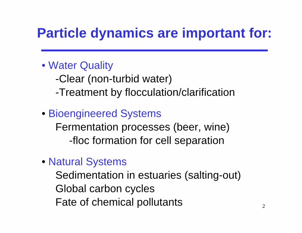
Particle dynamics are important for:

• Water Quality-Clear (non-turbid water)-Treatment by flocculation/clarification

• Bioengineered SystemsFermentation processes (beer, wine)

-floc formation for cell separation

• Natural SystemsSedimentation in estuaries (salting-out)Global carbon cyclesFate of chemical pollutants

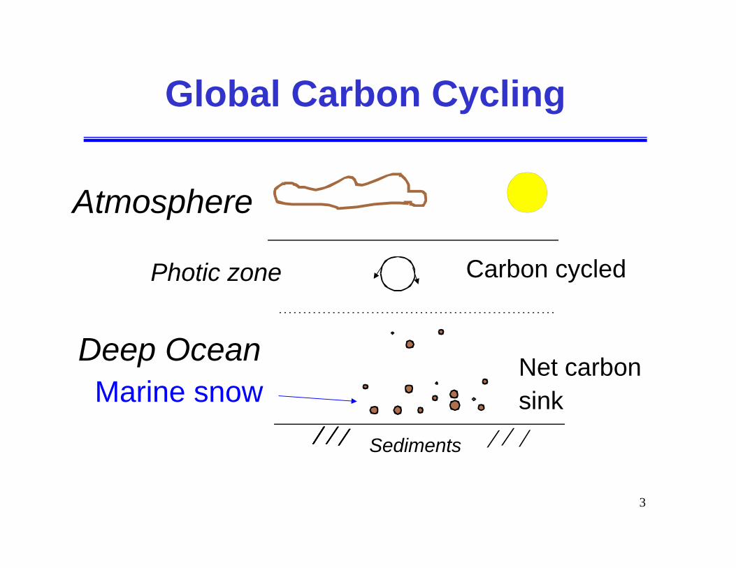
3

Net carbonsink

Deep OceanMarine snow

Carbon cycledPhotic zone

Global Carbon Cycling

Sediments

Atmosphere

4

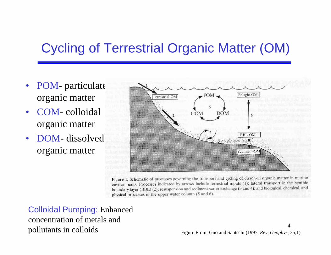
Cycling of Terrestrial Organic Matter (OM)

• POM- particulate organic matter

• COM- colloidal organic matter

• DOM- dissolved organic matter

Figure From: Guo and Santschi (1997, Rev. Geophys, 35,1)

Colloidal Pumping: Enhanced concentration of metals and pollutants in colloids

5Gustafsson&Gschwend, Limnol. Oceanogr. 1997, 42, 519.

Metals (and other pollutants) can partition onto particles to different extents

6

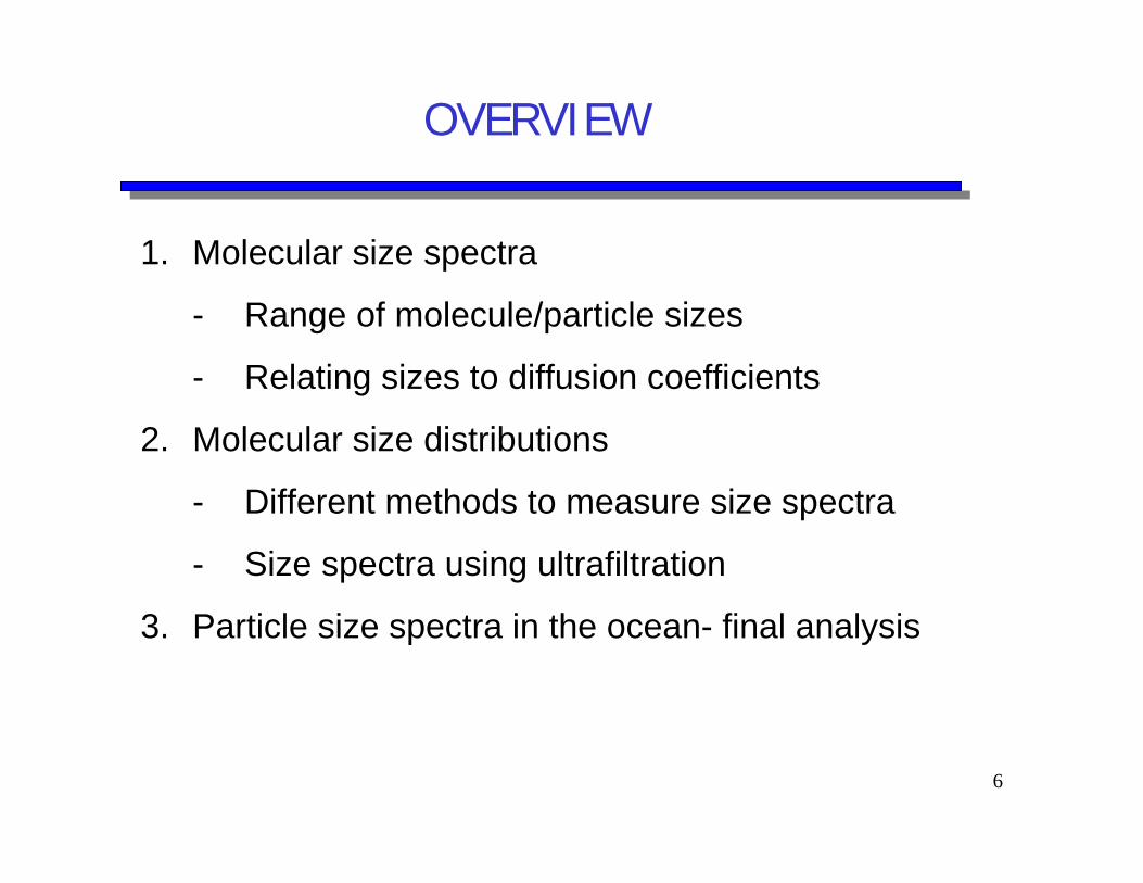
OVERVIEW

1. Molecular size spectra

- Range of molecule/particle sizes

- Relating sizes to diffusion coefficients

2. Molecular size distributions

- Different methods to measure size spectra

- Size spectra using ultrafiltration

3. Particle size spectra in the ocean- final analysis

7

8

Molecular Size Distributions

• Molecules: approximately <1000 Daltons (<1 kD)– Known structure– Tabulated values, correlations, measurements

• Macromolecules: >1 kD– Colloids of known properties; sometimes known structure– Proteins, polysaccharides, etc.– Humic and fulvic acids sometimes included – Correlations and measurement

• Colloids: >1 kD to < 0.2 um– Unknown properties– Must be experimentally measured.

9

A diffusion coefficient is the fundamental property needed for particle transport

• Chemical flux (J) is related to the concentration gradient according to

(General Form) (One dimension)

• Flux is in the opposite direction to the gradient• Diffusion coefficient in water is primarily a

property of molecule size and shape.

dxdcDJ cDJ

10

Relating Molecule Size, Molecular Weight, and Diffusivity

Diameter (nm)

Molecular weight (Daltons)

Diffusivity (×108cm2s-1)

13. 1,000,000 25 6.2 100,000 50 2.9 10,000 110 1.3 1,000 250

0.62 100 700

11

Diffusion Coefficients: Relating Molecule Size to Diffusivity

• Size of molecule• Viscosity of water• Intermolecular forces

Most important factors:

Where:

DCw= diffusion coefficient of chemical C in water (cm2/s)

kB=Boltzman’s constant= 1.3810-23 kgm2/s2K

= dynamic viscosity= 1 cp = 0.01 g/s-cm

T= temperature [K]

r = molecule radius

• Creeping flow (Re<<1)

• Spherical particles

• No slip at surface

Assumptions

Stokes-Einstein equation

rTkD B

Cw 6

At 20oC in water DCW [cm2/s]= 2.14×10-9 r-1 [µm]

12

Diffusivities from Structure: MOLECULES

Wilke-Chang Correlation

Where: [these units must be used]

DCw= diffusion coefficient [cm2/s]

T= temperature [K]

l= association parameter [ ]

Ml= molecular weight of liquid [g/mol]

= dynamic viscosity [cp]

VC,b= molal volume at normal boiling point [cm3]

6.0,

2/18 )(104.7

bC

llCw V

MTD

87.1, )(27.0 llbC MV

Only if:

359, bCVOnly if:

6.0,

42 1048.1]/[ bCCw VscmDFor chemicals in water: 20oC, =2.6, M=18 g/mol

13

The atomic volume can be estimated knowing the structure of the molecule

Example: Glucose (C6H12O6)

VG,b= 166.2 [cm3/g]

VG,b=(614.8)+(123.7)+(57.4) + (111) - 15

6.0,

42 )2.166(1048.1]/[ bGCw scmD

6.0,

42 1048.1]/[ bCCw VscmD

82 1090.6]/[ scmDCw

)%13(1080.7]/[ 82 errorscmDCwReported

14

Diffusivities from Size: MACROMOLECULES

HUMIC & FULVIC ACIDS

Beckett Correlation

47.052 1004.7]/[ DCw MscmDOnly if: M>1 kD

3/152 1074.2]/[ pCw MscmD

POLYSACCHARIDES

(Dextrans)

Frigon Correlation

Only if: M>1 kD

PROTEINS

Polson Correlation

422.042 1042.1]/[ HCw MscmDNatural organic matter (NOM)

15

Comparison of Diffusion coefficients for Polysaccharides (Dextrans) and Proteins

16

How do we easily account for temperature?

Take the Wilke-Chang correlation, 6.0

,

2/18 )(104.7

bC

llCw V

MTD

Rearranging, so that for one chemical all constants are on one side of the equation

constant)(104.76.0

,

2/18

bC

llCw

VM

TD

TTDD T

TCwTCw

,Or more simply,

So know we can write that at some new temperature T, we have from knows at a previous temperature,

constant, T

TTCwCw

TD

TD

17

Molecular Size Distributions: COLLOIDS

• We know the structure of a very small fraction of dissolved organic matter (DOM)

• Most oceanographers classify colloids as DOM >1 kD• Does size of molecules matter? YES

– Biodegradability (bacteria must hydrolyze if >1 kD)– Removal in water treatment processes (adsorption)

• To relate size to diffusivity, use Stokes-Einstein (SE) equation.

• To relate molecular weight to size (or diffusivity), must have calibration standards (i.e. synthentic molecules, proteins, dextrans, etc.)

18

Diffusion coefficients: homogeneous particle size

• Force on a particle of mass mc due to gravity is F=mcg

• In a centrifuge spinning at , F=mc2r, where r=distance from center

• From the velocity of particle during centrifugation (incorporated int the “s”term), it is possible to calculate the diffusivity :

• Analysis of the particle is used to determine the radius of gyration, rg

• Modified form of SE equation is used.

Light ScatteringUltracentrifugation

)1( wCcCw Vm

RTsD

cg is a new coefficient

• For DOM in water, we have:152 1069.1]/[ OO rscmD

gg

BCw rc

TkD6

19

Size Exclusion Chromatography (SEC)

Water from Lake Huron

Humic Acid (Aldrich)

Fulvic acid (Contec)

•Molecules separated by exclusion of larger particle

•Smaller particles diffuse into porous particles in column, and are delayed

•Can use low pressure (gel permeation chromatography; GPC) or high pressure chromatography (HPLC-SEC).

20

Field Flow Fractionation

Molecules are separated using two methods, based on:

•Molecule size (like SEC)

•Another method acting perpendicular to the direction of flow, such as an electric or fluid field

21

Ultrafiltration (UF)• Membranes fabricated that have set average pore size• Rated in terms of atomic mass units (amu) or Daltons

based on >99% rejection of molecules larger than the stated amu.

• UF separations provide discrete (not continuous) molecular size distributions

• There is no “perfect” membrane. Problems are:– Some materials are rejected due to charge repulsion– Build up of material on membrane can cause rejection of smaller

sized molecules– Most researchers incorrectly report sizes by not considering

membrane rejection (Apparent size distribution)– The Actual size distribution can be determined using a

permeation coefficient model.

22

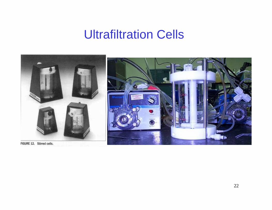
Ultrafiltration Cells

23

UF Cell Components

Ultrafiltration cell body

Stirrer used to mix retentateand minimize fouling

UF membrane

Permeate

Cell is pressurized to drive out permeate

Retentate

24

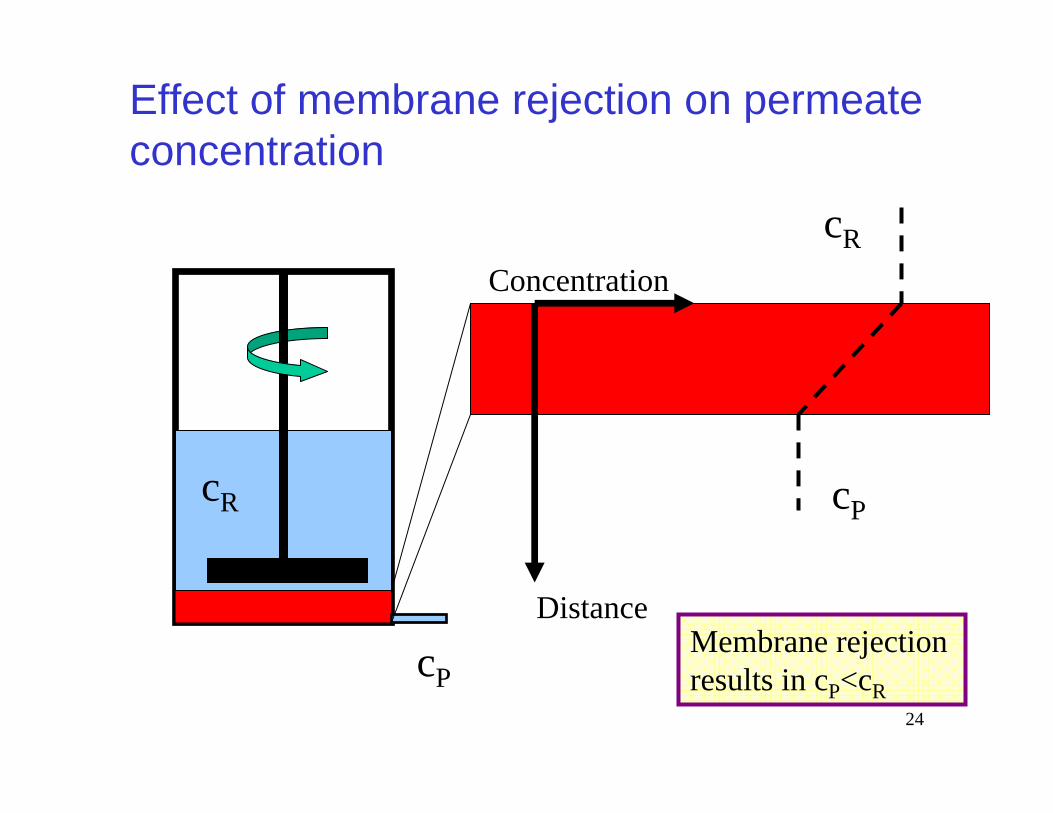
Effect of membrane rejection on permeate concentration

Concentration

Distance

cR

cP

cR

cP

Membrane rejection results in cP<cR

25

Mass Balance Equations Produce Fundamental Relationships

Permeate concentration at at any time

Filtrate Concentration (all of the permeate is collected)

)1()1(

0, FFcc

cp

rf

10,

cprcP Fcpc

cr,0= concentration of material able to pass the membrane

F= fraction of filtrate removed [F=1-(Vf/Vr,0)]

pc= permeation coefficient

26

…derivation of equations…

27

Examples of UF Size Separations

• Example permeation coefficient model calculation to determine concentration of material <1K in sample using UF size separation.

•Separation of compounds having a known molecular weight using a 1000 amu membrane

• Vitamin B-12: MW=1192 Daltons• Sucrose: MW=342 Daltons

•Errors for values of the permeation coefficient

•Effect of parallel versus serial filtration

28

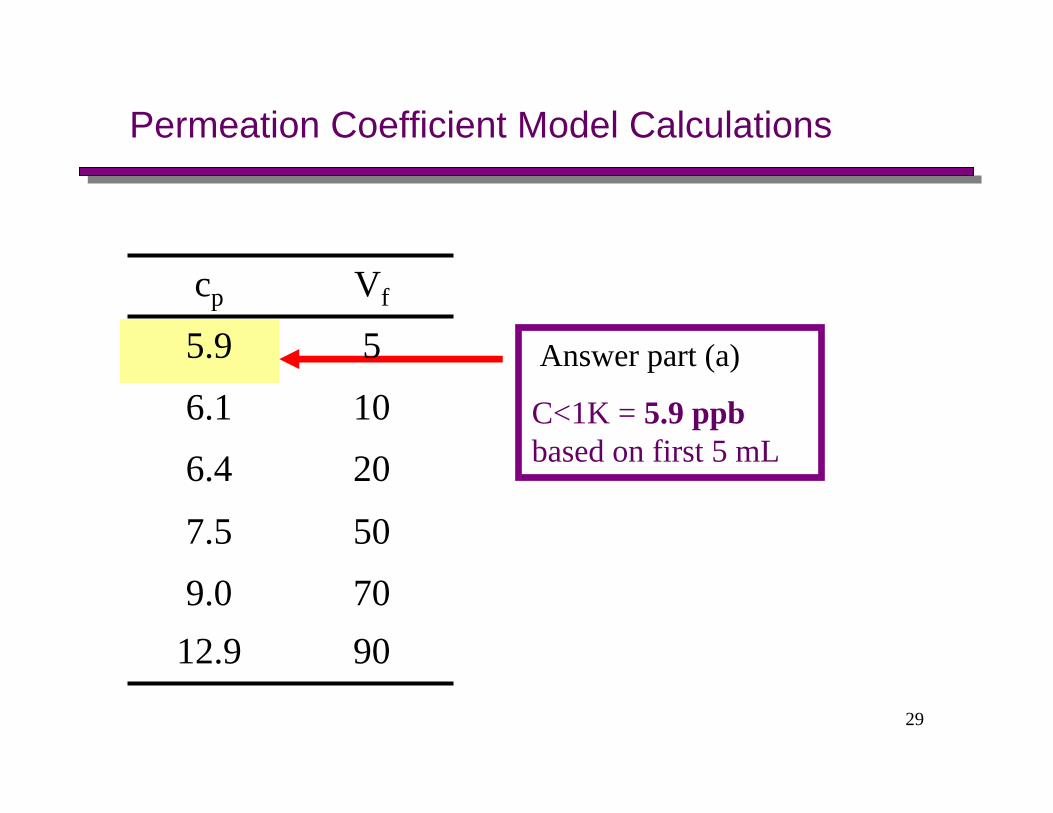
Example: UF Separation, 1K amu

• You wish to determine the concentration of DOC (ppb) in seawater that is <1000 Daltons (C<1K). You use a 1K cell filledwith 100 mL of sample.

•Permeate concentrations are measured at 6 times during separation.

Based on the following approaches, what would you conclude is the concentration of material <1K in the sample (C<1K)?

a) Apparent C<1K based on the first measurement (the instantaneous permeate sample at 5 mL)?

b) True C<1K based on the permeate coefficient model?

c) Apparent C<1K based on collecting 90 mL?

29

Answer part (a)

C<1K = 5.9 ppbbased on first 5 mL

Permeation Coefficient Model Calculations

9012.9709.0

507.5

206.4

106.1

55.9

Vfcp

30

Permeation Coefficient Model Calculations

0.19012.9

0.3709.0

0.5507.5

0.8206.4

0.90106.1

0.9555.9

FVfcp)/(1 0,rf VVF

Vr,0=100 mL

31

Permeation Coefficient Model Calculations

0.19012.9

0.3709.0

0.5507.5

0.8206.4

0.90106.1

0.9555.9

FVfcp

Next step:

Take natural log of F and cp

32

Permeation Coefficient Model Calculations

-2.302.560.19012.9

-1.202.190.3709.0

-0.692.010.5507.5

-0.221.860.8206.4

-1.051.810.90106.1

-0.571.770.9555.9

ln Fln cpFVfcp

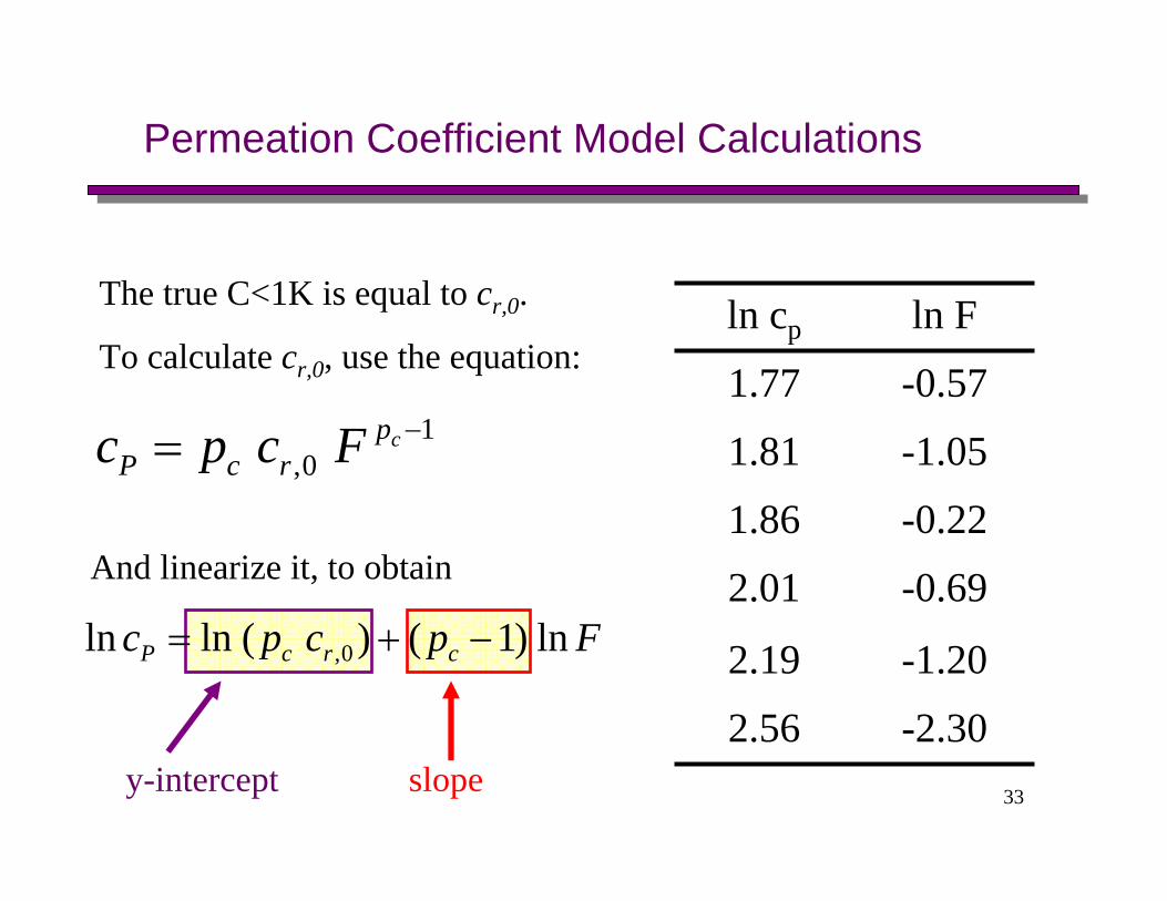
33

Permeation Coefficient Model Calculations

-2.302.56

-1.202.19

-0.692.01

-0.221.86

-1.051.81

-0.571.77

ln Fln cpThe true C<1K is equal to cr,0.

To calculate cr,0, use the equation:

10,

cprcP Fcpc

Fpcpc crcP ln)1()(lnln 0,

And linearize it, to obtain

slopey-intercept

34

Cr,0=e1.77/0.66=9.0

pc=(1-0.34)=0.66

Fpcpc crcP ln)1()(lnln 0,

Permeation Coefficient Model Calculations

34.094.5 FcP

Slope= 0.34

y-intercept=1.77y = 0.34 x + 1.77

R2 = 0.999

0

0.5

1

1.5

2

2.5

3

0 0.5 1 1.5 2 2.5

- ln F

ln c

p

Answer part (b)

Actual C<1K = 9.0 ppb

(Note sign change on ln F term)

35

Permeation Coefficient Model Calculations

What if the first 90 mL are used to determine C<1K?

8.7fc

1.0)100/90(1)/(1 0, rf VVFIf 90 mL are collected, then F is:

)1()1(0.9

)1()1( 66.0

0, FF

FFcc

cp

rf

)1.0(1))1.0(1(0.9

66.0

fc

Answer part (c)

C<1K = 7.8 ppb based on 90 mL

36

Permeation Coefficient Model: Comparison

13%7.8Collect 90 of 100 mL

---9.0Permeation Coefficient Model

44%5.9Collect 5 mL

ErrorC <1K (ppb)Method

37

Effect of different filtration volumes on apparent C (<1k)

Time (or Vf)

Cp

C(<1K)

C(<1K)

C(<1K)

38

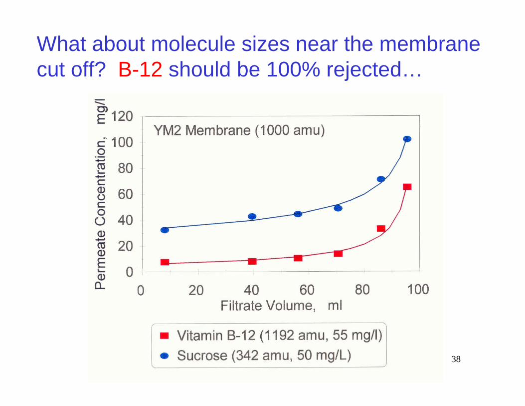
What about molecule sizes near the membrane cut off? B-12 should be 100% rejected…

39

pc-values are very low for B-12

40

Error analysis of pc values

Error of concentration of chemical A in a two component (A, B) system,

pc (A) is fixed as shown

pc (B) varies (0.1, 0.3, 0.5, 0.7, 0.9)

pc(A)=0.5

pc(A)=0.3

Errors are large when pc=0.1

Only use pc correction if pc>0.2

41

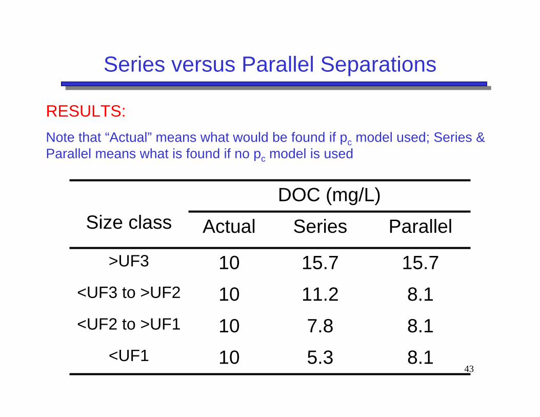
Series versus Parallel Separations

42

Series versus Parallel Separations

• Examine separations through membranes UF1, UF2, and UF3, each one having a different molecular weight cut off (UF3 has the highest cut off, for example 100K).

• Assume there is 10 mg/L of DOC in each size fraction.

• Compare results for series versus parallel analysis of the sample.

43

Series versus Parallel Separations

RESULTS: Note that “Actual” means what would be found if pc model used; Series & Parallel means what is found if no pc model is used

8.15.310<UF1

8.17.810<UF2 to >UF1

8.111.210<UF3 to >UF2

15.715.710>UF3

ParallelSeriesActualDOC (mg/L)

Size class

44

Notes on UF size separations

• Apply the permeation coefficient model unless:– pc>0.9 (little rejection by membrane)– pc<0.2 (sizes are too close to membrane cutoff)

• Prepare size fractions in parallel, not serial

• When size distributions are adjusted for membrane rejection, mass will be shifted to smaller size fractions

45

RESULTS of Actual Water Samples

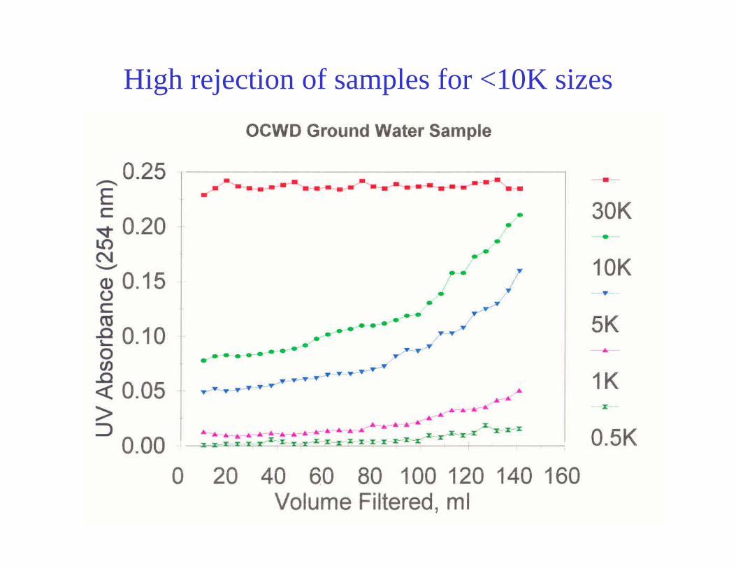
•Size distributions of NOM in groundwater using UV-absorbance (indicating concentration of humic and fulvicacids)

•Orange county ground water (OCWD)•Biscayne aquifer ground water

•Dissolved Organic Carbon in Wastewater

•Molecular weight distributions of pure compounds during bacterial degradation in pure and mixed cultures.

46

47

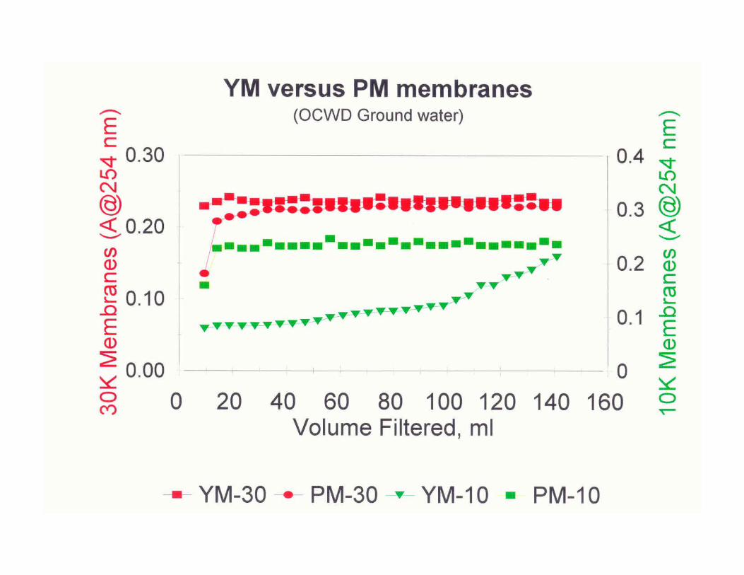
High rejection of samples for <10K sizes

48

Adjusting the size distribution with the pc model shifts the distribution to smaller MW

49

Size distributions during bacterial degradation of Protein macromolecules

Small MW compounds doaccumulate with proteins with

pure cultures

Small MW compounds do notaccumulate with proteins with

mixed cultures

Pure cultures Mixed cultures

50

Size distributions during bacterial degradation of dextran macromolecules: Mixed cultures

Small MW compounds

do accumulate

with dextrans(mixed or

pure cultures)

51

Continuous flow method for molecular size distributions

• In some systems, organic matter concentrations are very low (e.g. seawater) and must be conentrated to be measured.

• A continuous flow method was developed for this situation.

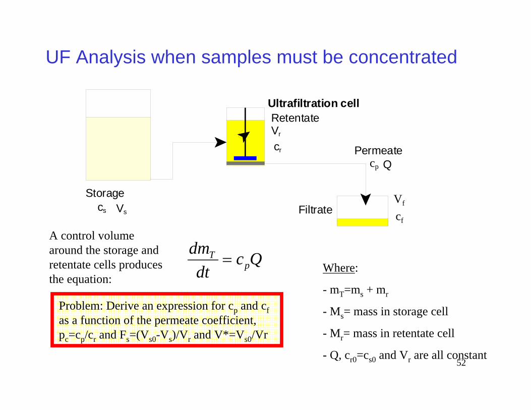
52

UF Analysis when samples must be concentrated

Qcp

Vr

Vf Filtrate

Permeate

Ultrafiltration cell

Storage

cf

Retentate

cr

cs Vs

A control volume around the storage and retentate cells produces the equation:

Qcdt

dmp

T

Problem: Derive an expression for cp and cfas a function of the permeate coefficient, pc=cp/cr and Fs=(Vs0-Vs)/Vr and V*=Vs0/Vr

Where:

- mT=ms + mr

- Ms= mass in storage cell

- Mr= mass in retentate cell

- Q, cr0=cs0 and Vr are all constant

53

ANSWERS

UF Analysis when samples must be concentrated

Qcp

Vr

Vf Filtrate

Permeate

Ultrafiltration cell

Storage

cf

Retentate

cr

cs Vs

scFpccc

sf eppp

VVcc

)1(111*

*0

scFpcsp epcc )1(10

54

UF Results: Comparison of Storage Reservoir vs Batch Approaches

Figures from: Cai, 1999, Water Res., 33, 13.

Batch SampleStorage Reservoir