Gh.niculescu, Ifrim, Diaconescu, 1987, Chirurgia Traumatismelor Osteoarticulare
Romanian Journal of Economic Forecasting – XVIII (3) 2015 5
EASTERN EUROPE IN THE WORLD
ECONOMY: A GLOBAL VAR ANALYSIS
Moisă ALTĂR1 Adrian IFRIM2
Adam-Nelu ALTĂR - SAMUEL3
Abstract
This paper investigates the effects of international shocks on three Eastern European emerging countries: Romania, Hungary and Poland, over the period 1998Q2-2011Q2 using a GVAR model. Evidence based on the GVAR model showed the importance of second and higher order effects, in the international transmission mechanism of shocks from the U.S. to Eastern European countries. The results of generalized impulse response functions (GIRFs) suggest that the U.S. equity shocks are transmitted very fast to others markets and that the Eastern European equity markets tend to overshoot the U.S. response. The U.S. adverse equity and output shocks revealed asymmetric responses and greater volatility of real exchange rates in the countries of Eastern Europe compared to the Euro Area, suggesting a “flight to quality” from emerging to developed economies. At the same time, the shocks originating from the Euro Area have limited effects on the countries of focus, and tend not to be amplified over time, implying that the effects of shocks could be compensated among the members of the region. Keywords: GVAR, emerging markets, spillovers, global interdependencies, impulse
responses JEL Classification: C32, F42, F44, O52
1. Introduction
The increased integration and interdependence in the world economy as a result of expanding trade, investment and international financial services have important consequences for the national business cycles and the transmission of shocks between countries. Such discussions are based on the stylized fact that the recent global economic crisis has emphasized the existence of a world business cycle, in which 1 The Bucharest University of Economic Studies, The Romanian - American University – FINSYS,
E-mail: [email protected]. 2 The Romanian – American University - FINSYS , E-mail: [email protected]. 3 The Romanian – American University, Bucharest, Romania, E-mail: [email protected].
1.
Institute for Economic Forecasting
Romanian Journal of Economic Forecasting –XVIII (3) 2015 6
business cycles across countries display patterns of co-movement of output, inflation, interest rates and real equity prices. As a result, the national economic issues should be considered from a global perspective. In recent years, Pesaran et al. (2004), Dees et al. (2007a) and Dees et al. (2007b) have developed a method for evaluating the international linkages, by combining time series, panel data and factor analysis techniques. In the first step of the methodology, vector error-correction models are estimated individually for each country in which domestic variables are related to foreign specific variables and, possibly, with global variables. These country-specific foreign variables are treated as weakly exogenous and constructed as a weighted average of other countries specific variables. In the second step, all country-specific error-correction models are combined using a link matrix of predetermined cross-country linkages. Unlike standard VAR’s, which treat all variables as endogenous, the GVAR allows for addressing the “curse of dimensionality” problem by treating the foreign variables as weakly exogenous and, thus, permitting to estimate country specific models individually. The aim of this paper is to explore the international transmission mechanism of global shocks to the emerging countries in Eastern Europe and to analyze the international economic linkages between three Eastern European emerging economies: Romania, Hungary and Poland, and the rest of the world. The GVAR model accounts for a large number of international relations across macroeconomic and financial variables and, thus, allows for studying how a shock to a macroeconomic variable in one country may affect the economic condition of other countries. Due to the importance of the U.S. in the world economy and the importance of the Euro Area for the considered countries, most of the shocks will originate there. To investigate the transmission of shocks, generalized impulse response functions (GIRFs) are used. The GIRFs, developed by Koop, Pesaran and Potter (1996), and Pesaran and Shin (1998), take into account the contemporaneous correlation among the error terms in the GVAR model. The focus of the analysis is on impulse response functions generated by a shock to the U.S. real output, a shock to the U.S. real equity prices and a shock to the U.S. interest rates. Furthermore, a shock to the Euro Area real output is considered. It is important to note that the shocks considered in this analysis are not structural. However, given the focus of the paper, which is the study of the international transmission mechanism of shocks to the emerging countries in Eastern Europe, the identification of shocks is not critical in the present study. The specification of the GVAR model used in this paper closely follows the one in Dees et al. (2007a). In addition, we use a bootstrap procedure to study the significance of the GIRFs. The contribution of this paper is twofold. First, to our knowledge, this is the first GVAR model to assess the individual effects of international shocks on the macroeconomic variables of the Eastern European countries. The emphasis is on individual because in contrast to the paper of Yan Sun et al. (2013), which studies the effects of shocks to the CESEE countries modeled as regions, this paper considers individual specification for the countries from Eastern Europe. Secondly, due to individual specification of the Eastern European countries, some asymmetric responses could be observed between the emerging and developed economies. The effects of an adverse shock to the U.S. real output revealed that while the real exchange rates in the developed countries tended to appreciate, the real exchange rates in Eastern Europe
Eastern Europe in the World Economy: A Global VAR Analysis
Romanian Journal of Economic Forecasting – XVIII (3) 2015 7
suffered a massive depreciation. This asymmetric response could be interpreted as a flight to quality. Furthermore, the same pattern was also observed in the case of a fall in the U.S. equity prices. The rest of the paper is organized as follows: section two presents the GVAR model and its dynamic properties, section three describes the econometric methodology, section four illustrates the effects of international shocks on the macroeconomic variables from Eastern European countries and the final section concludes.
2. The GVAR Model
The GVAR model is a global model that combines many individual country models. Each country is treated as a small open economy by estimating country specific error-correction models in which domestic variables are dependent on foreign and global variables. The foreign variables are treated as weakly exogenous, a property that will be tested in this paper. After the country specific models are estimated, they are linked together by a matrix of predetermined (not estimated) cross-country linkages. In this paper, the trade weights will be used to compute the link matrix, in line with Pesaran et al. (2004), Dees et al. (2007a), Cesa-Bianchi et al. (2012).
2.1. Country-specific Models Consider N + 1 countries (or regions) in the global economy indexed by i = 0, 1, 2, … , N. Country 0 is the reference country, which in this case, as well as in the GVAR literature, it is the U.S. (the choice is obvious taking into account that the U.S. is still the dominant country in the global economy). With the exception of country 0, all the other N countries are modelled as small open economies in which domestic variables ( itx )
are related to country-specific foreign variables ( *itx ) ` as weighted averages of
endogenous variables from other countries, plus global variables (e.g. oil price, food price) and deterministic variables such as time trends. Confining the model to a first order dynamic specification, where the 1ik country specific domestic variables, itx ,
are related to the 1* ik vector of foreign variables, *itx , we can write the following
VARX*(1,1) model for country i: (1)
where: 0ia is a 1ik vector of intercepts, i is a ii kk matrix of lagged coefficients,
0i and 1i are *ii kk matrix of coefficients associated with foreign variables, and
it is a 1ik vector of country-specific shocks. Moreover, the idiosyncratic shocks are assumed to be serially uncorrelated, with zero mean and non-singular covariance matrix.
NiTtxxxtaax ittiiititiiiiit
,...2,1,0;,...,2,1
*1,1
*01,10

Institute for Economic Forecasting
Romanian Journal of Economic Forecasting –XVIII (3) 2015 8
The foreign variables, *itx ,, play a crucial role in the GVAR model. The vector of foreign
variables is constructed as a weighted average of other countries variables:
N
jkjtijkit xwx
0
* , 0iiw , N
jijw 1 (2)
where: *kitx is the thk domestic variable from the vector of foreign variables *
itx , and
the weights ijw are constructed as the share of country j in the trade (imports plus
exports) of country i , namely ii
ji
ji
ij EXIMEXIM
w
, where jiIM and j
iEX represent the
import and export of country i with country j , and iIM , iEX represent the total import and export of country i .The weights are not estimated, but instead they are specified a priori in order to deal with the “curse of dimensionality”. Figure 1 shows the dynamics of world trade, percent of GDP, and of world real GDP (base year 2005), both expressed in rates of growth. It is clear that the severe hit to the global trade was one of the main sources of transmission of the economic crisis worldwide, which lends further support to the use of trade-based weights in the construction of foreign specific variables.
Figure 1 Global Trade and Real GDP
’ Source: World Bank, authors’ computations.
2.2. Building the Global VAR Model The GVAR model is obtained by combining all the country-specific VARX* models and linking them with a matrix of predetermined trade weights. Following Pesaran et al. (2004), by stacking all the variables in country i , we define the 1)( * ii kk vector
*, ititit xxz . Equipped with this, relation (1) can be rearranged to obtain
-0,2
-0,1
0
0,1
0,2
2001 2002 2003 2004 2005 2006 2007 2008 2009 2010 2011 2012
Real GDP Trade

Eastern Europe in the World Economy: A Global VAR Analysis
Romanian Journal of Economic Forecasting – XVIII (3) 2015 9
ittiiiiiti zBtaazA 1,10 (3)
with ),( 0iki iIA and ),( 1iiiB , both of dimension )( *
iii kkk . Stacking all
the endogenous variables from all countries in a vector ),.....,,( ''1
'0 Ntttt xxxg of
dimension
N
iikk
0, and taking into account that foreign variables are weighted avera-
ges of domestic ones, relation (3) can be written in terms of the global vector tg a
tiit gLz , Ni ,....,2,1,0 (4) where the matrix iL , of dimension kkk ii )( * , contains the fixed country-specific bilateral trade weights. Using this fact, (4) can now be rewritten in terms of the global vector tg :
ittiiiitii gLBtaagLA 110 (5) Stacking all the country-specific VARX* models together yields the global model ttt MgtaaGg 110 . (6) Furthermore, a global variable (common to all countries, e.g. the oil price) could be introduced in the initial VARX* models. Such a model is given by
ttttt ddFgtg 110110 (7)
where: td is a 1c vector of global variables assumed to be weakly exogenous and
01
0 aG , 11
1 aG , MGF 1 01
0 G , 11
1 G , .1tt G
The GVAR model given by (7) can be solved recursively and its dynamic properties can be analyzed using generalized impulse response functions (GIRFs). The dynamic properties of the GVAR model are closely related to the eigenvalues of the F matrix. Anticipating the discussion in the next section, the stability of the model is assured when the eigenvalues of the matrix F lie on or inside the unit circle4. The unit eigenvalues correspond to the cointegration relationships in the global model. In order to capture the short-run, as well as the long-run relations in the global economy, and due to the fact that the variables included in the model are integrated of order 1 (as detailed in section 3.2), we estimate the models in the error-correction form :
ititiitiiiiiiit xtvzvax *
01,0 )]1([ . (8)
where iiiii BA )( . One should notice that we restricted the trend coefficients to lie in the cointegration space by imposing iii va 1
5.
4 As noted in Pesaran et al. (2004), besides the stability condition, the validity of the GVAR model
is assured if i) the weights are relatively small; ii) cross-dependence of shocks is small. 5 See Pesaran, Shin and Smith (2000).
Institute for Economic Forecasting
Romanian Journal of Economic Forecasting –XVIII (3) 2015 10
3. A GVAR Model for Eastern European Countries in the Global Economy
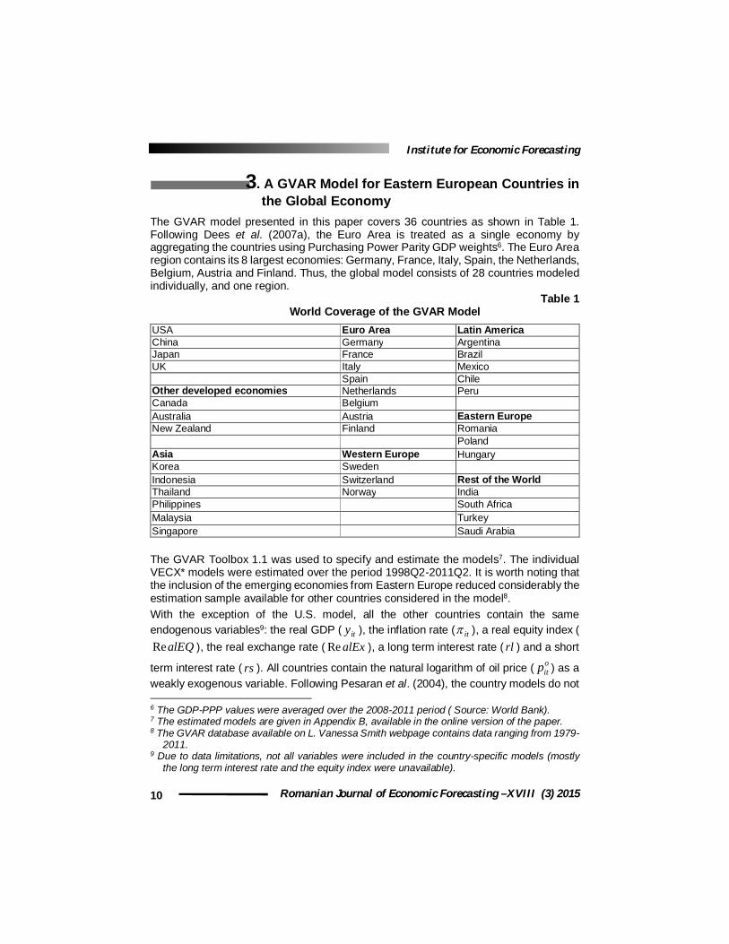
The GVAR model presented in this paper covers 36 countries as shown in Table 1. Following Dees et al. (2007a), the Euro Area is treated as a single economy by aggregating the countries using Purchasing Power Parity GDP weights6. The Euro Area region contains its 8 largest economies: Germany, France, Italy, Spain, the Netherlands, Belgium, Austria and Finland. Thus, the global model consists of 28 countries modeled individually, and one region.
Table 1 World Coverage of the GVAR Model
USA Euro Area Latin America China Germany Argentina Japan France Brazil UK Italy Mexico Spain Chile Other developed economies Netherlands Peru Canada Belgium Australia Austria Eastern Europe New Zealand Finland Romania Poland Asia Western Europe Hungary Korea Sweden Indonesia Switzerland Rest of the World Thailand Norway India Philippines South Africa Malaysia Turkey Singapore Saudi Arabia
The GVAR Toolbox 1.1 was used to specify and estimate the models7. The individual VECX* models were estimated over the period 1998Q2-2011Q2. It is worth noting that the inclusion of the emerging economies from Eastern Europe reduced considerably the estimation sample available for other countries considered in the model8. With the exception of the U.S. model, all the other countries contain the same endogenous variables9: the real GDP ( ity ), the inflation rate ( it ), a real equity index (
alEQRe ), the real exchange rate ( alExRe ), a long term interest rate ( rl ) and a short
term interest rate ( rs ). All countries contain the natural logarithm of oil price ( oitp ) as a
weakly exogenous variable. Following Pesaran et al. (2004), the country models do not 6 The GDP-PPP values were averaged over the 2008-2011 period ( Source: World Bank). 7 The estimated models are given in Appendix B, available in the online version of the paper. 8 The GVAR database available on L. Vanessa Smith webpage contains data ranging from 1979-
2011. 9 Due to data limitations, not all variables were included in the country-specific models (mostly
the long term interest rate and the equity index were unavailable).
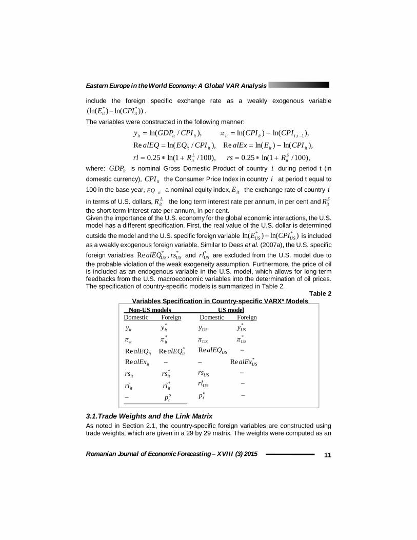
Eastern Europe in the World Economy: A Global VAR Analysis
Romanian Journal of Economic Forecasting – XVIII (3) 2015 11
Non-US models US model Domestic Foreign Domestic Foreign
ot
itit
itit
it
itit
itit
itit
p
rlrl
rsrs
alExalEQalEQ
yy
*
*
*
*
*
ReReRe
ot
US
US
US
US
USUS
USUS
p
rlrs
alEx
alEQ
yy
*
*
*
Re
Re
include the foreign specific exchange rate as a weakly exogenous variable ))ln()(ln( **
itit CPIE . The variables were constructed in the following manner:
),100/1ln(25.0 ),100/1ln(25.0),ln()ln(Re ),/ln(Re
),ln()ln( ),/ln( 1,
Sit
Lit
itititit
tiititititit
RrsRrlCPIEalExCPIEQalEQ
CPICPICPIGDPy
where: itGDP is nominal Gross Domestic Product of country i during period t (in domestic currency), itCPI the Consumer Price Index in country i at period t equal to 100 in the base year, itEQ a nominal equity index, itE the exchange rate of country iin terms of U.S. dollars, L
itR the long term interest rate per annum, in per cent and SitR
the short-term interest rate per annum, in per cent. Given the importance of the U.S. economy for the global economic interactions, the U.S. model has a different specification. First, the real value of the U.S. dollar is determined outside the model and the U.S. specific foreign variable )ln()ln( **
USUS CPIE is included as a weakly exogenous foreign variable. Similar to Dees et al. (2007a), the U.S. specific foreign variables ** ,Re USUS rsalEQ and *
USrl are excluded from the U.S. model due to the probable violation of the weak exogeneity assumption. Furthermore, the price of oil is included as an endogenous variable in the U.S. model, which allows for long-term feedbacks from the U.S. macroeconomic variables into the determination of oil prices. The specification of country-specific models is summarized in Table 2.
Table 2 Variables Specification in Country-specific VARX* Models
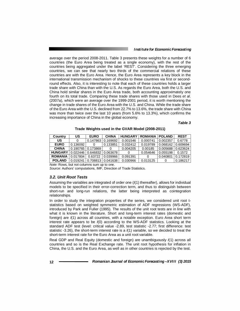
3.1.Trade Weights and the Link Matrix As noted in Section 2.1, the country-specific foreign variables are constructed using trade weights, which are given in a 29 by 29 matrix. The weights were computed as an
Institute for Economic Forecasting
Romanian Journal of Economic Forecasting –XVIII (3) 2015 12
average over the period 2008-2011. Table 3 presents these weights for a number of 6 countries (the Euro Area being treated as a single economy), with the rest of the countries being aggregated under the label ‘REST’. Considering the three emerging countries, we can see that nearly two thirds of the commercial relations of these countries are with the Euro Area. Hence, the Euro Area represents a key block in the international transmission mechanism of shocks to these countries via first or second-round effects. Also, it is interesting to note that each of these countries holds a larger trade share with China than with the U.S. As regards the Euro Area, both the U.S. and China hold similar shares in the Euro Area trade, both accounting approximately one fourth on its total trade. Comparing these trade shares with those used in Dees et al. (2007a), which were an average over the 1999-2001 period, it is worth mentioning the change in trade shares of the Euro Area with the U.S. and China. While the trade share of the Euro Area with the U.S. declined from 22.7% to 13.6%, the trade share with China was more than twice over the last 10 years (from 5.6% to 13.3%), which confirms the increasing importance of China in the global economy.
Table 3 Trade Weights used in the GVAR Model (2008-2011)
Country US EURO CHINA HUNGARY ROMANIA POLAND REST
US 0 0.147863 0.169692 0.001546 0.000741 0.002357 0.6778 EURO 0.136092 0 0.133851 0.032412 0.019789 0.068162 0.609694 CHINA 0.190765 0.173869 0 0.004205 0.00185 0.005688 0.623624
HUNGARY 0.022446 0.646832 0.063678 0 0.054646 0.055198 0.1572 ROMANIA 0.017804 0.63722 0.039966 0.091391 0 0.040801 0.172819 POLAND 0.019241 0.708813 0.041638 0.030966 0.013125 0 0.186217
Note: Rows, but not columns sum up to one. Source: Authors’ computations, IMF, Direction of Trade Statistics.
3.2. Unit Root Tests Assuming the variables are integrated of order one (I(1) thereafter), allows for individual models to be specified in their error-correction term, and thus to distinguish between short-run and long-run relations, the latter being interpreted as cointegration relationships. In order to study the integration properties of the series, we considered unit root t-statistics based on weighted symmetric estimation of ADF regressions (WS-ADF), introduced by Park and Fuller (1995). The results of the unit root tests are in line with what it is known in the literature. Short and long-term interest rates (domestic and foreign) are I(1) across all countries, with a notable exception. Euro Area short term interest rate appears to be I(0) according to the WS-ADF statistics. Looking at the standard ADF test (level: critical value -2.89, test statistic -2.77; first difference: test statistic -3.26), the short-term interest rate is a I(1) variable, so we decided to treat the short-term interest rate for the Euro Area as a unit root variable. Real GDP and Real Equity (domestic and foreign) are unambiguously I(1) across all countries and so is the Real Exchange rate. The unit root hypothesis for inflation in China, the U.S. and the Euro Area, as well as in other countries is rejected by the test.
Eastern Europe in the World Economy: A Global VAR Analysis
Romanian Journal of Economic Forecasting – XVIII (3) 2015 13
Since overdifferencing is likely to be a less important specification error than wrongly including a I(2) variable, we decided to include inflation as an I(1) variable as in Pesaran et al. (2004). The same argument was applied to a small number of other variables from the emerging economies. Both WS-ADF and standard ADF tests seemed to suggest that domestic real output in India could be a I(2) variable, which is clearly implausible and could arise due to poor quality data or by chance. For the remaining countries and variables, the test results supported the assumption that the variables included in the models contain unit roots.
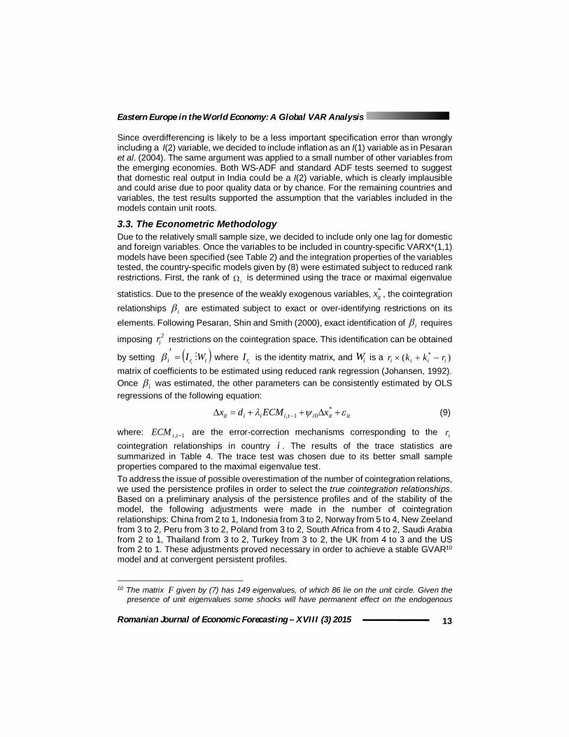
3.3. The Econometric Methodology Due to the relatively small sample size, we decided to include only one lag for domestic and foreign variables. Once the variables to be included in country-specific VARX*(1,1) models have been specified (see Table 2) and the integration properties of the variables tested, the country-specific models given by (8) were estimated subject to reduced rank restrictions. First, the rank of i is determined using the trace or maximal eigenvalue
statistics. Due to the presence of the weakly exogenous variables, *itx , the cointegration
relationships i are estimated subject to exact or over-identifying restrictions on its elements. Following Pesaran, Shin and Smith (2000), exact identification of i requires
imposing 2ir restrictions on the cointegration space. This identification can be obtained
by setting iri WIi where
irI is the identity matrix, and iW is a )( *iiii rkkr
matrix of coefficients to be estimated using reduced rank regression (Johansen, 1992). Once i was estimated, the other parameters can be consistently estimated by OLS regressions of the following equation:
itititiiiit xECMdx *
01, (9)
where: 1, tiECM are the error-correction mechanisms corresponding to the ir cointegration relationships in country i . The results of the trace statistics are summarized in Table 4. The trace test was chosen due to its better small sample properties compared to the maximal eigenvalue test. To address the issue of possible overestimation of the number of cointegration relations, we used the persistence profiles in order to select the true cointegration relationships. Based on a preliminary analysis of the persistence profiles and of the stability of the model, the following adjustments were made in the number of cointegration relationships: China from 2 to 1, Indonesia from 3 to 2, Norway from 5 to 4, New Zeeland from 3 to 2, Peru from 3 to 2, Poland from 3 to 2, South Africa from 4 to 2, Saudi Arabia from 2 to 1, Thailand from 3 to 2, Turkey from 3 to 2, the UK from 4 to 3 and the US from 2 to 1. These adjustments proved necessary in order to achieve a stable GVAR10 model and at convergent persistent profiles.
10 The matrix F given by (7) has 149 eigenvalues, of which 86 lie on the unit circle. Given the
presence of unit eigenvalues some shocks will have permanent effect on the endogenous
Institute for Economic Forecasting
Romanian Journal of Economic Forecasting –XVIII (3) 2015 14
Table 4 Number of Cointegration Relations in Individual VARX*(1, 1) Models
(Trace Statistics) Country CR Country CR
ARGENTINA 3 NORWAY 5 AUSTRALIA 2 NEW ZEELAND 3 BRAZIL 3 PERU 3 CANADA 2 PHILIPPINES 3 CHILE 3 POLAND 3 CHINA 2 ROMANIA 2 EURO 3 SOUTH AFRICA 4 HUNGARY 2 SAUDI ARABIA 2 INDIA 2 SINGAPORE 3 INDONESIA 3 SWEEDEN 2 JAPAN 1 SWITZERLAND 1 KOREA 2 THAILAND 3 MALAYSIA 3 TURKEY 3 MEXICO 2 UK 4 US 2
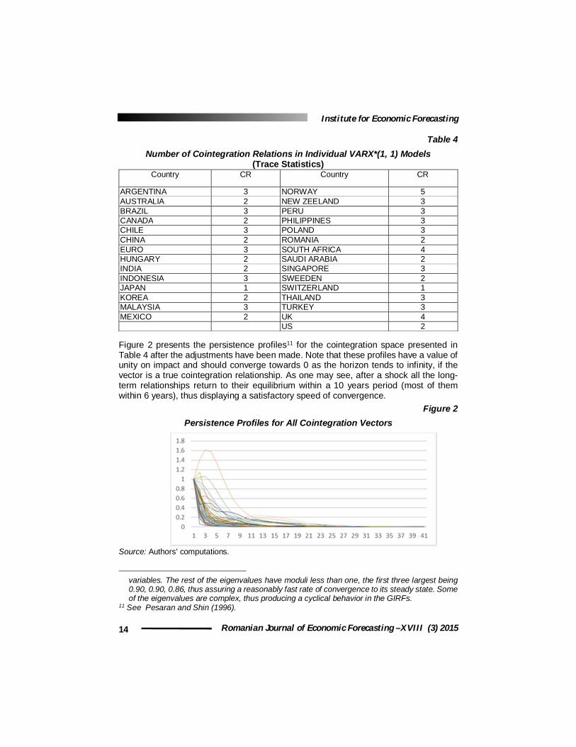
Figure 2 presents the persistence profiles11 for the cointegration space presented in Table 4 after the adjustments have been made. Note that these profiles have a value of unity on impact and should converge towards 0 as the horizon tends to infinity, if the vector is a true cointegration relationship. As one may see, after a shock all the long-term relationships return to their equilibrium within a 10 years period (most of them within 6 years), thus displaying a satisfactory speed of convergence. Figure 2
Persistence Profiles for All Cointegration Vectors
Source: Authors’ computations.
variables. The rest of the eigenvalues have moduli less than one, the first three largest being 0.90, 0.90, 0.86, thus assuring a reasonably fast rate of convergence to its steady state. Some of the eigenvalues are complex, thus producing a cyclical behavior in the GIRFs.
11 See Pesaran and Shin (1996).
0
0,5
1
1,5
2
1 3 5 7 9 11 13 15 17 19 21 23 25 27 29 31 33 35 37 39 41
Eastern Europe in the World Economy: A Global VAR Analysis
Romanian Journal of Economic Forecasting – XVIII (3) 2015 15
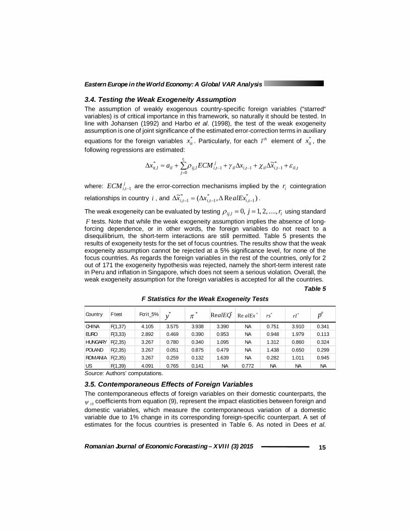
3.4. Testing the Weak Exogeneity Assumption The assumption of weakly exogenous country-specific foreign variables (“starred“ variables) is of critical importance in this framework, so naturally it should be tested. In line with Johansen (1992) and Harbo et al. (1998), the test of the weak exogeneity assumption is one of joint significance of the estimated error-correction terms in auxiliary equations for the foreign variables *
itx . Particularly, for each thl element of *itx , the
following regressions are estimated:
tiltiiltiil
r
j
jtilijillit xxECMax
i
,*
1,1,0
1,,*
,~
where: jtiECM 1, are the error-correction mechanisms implied by the ir cointegration
relationships in country i , and )Re,(~ *1,
*1,
*1, tititi alExxx .
The weak exogeneity can be evaluated by testing ilij rj ....,,2,1,0, using standard F tests. Note that while the weak exogeneity assumption implies the absence of long-forcing dependence, or in other words, the foreign variables do not react to a disequilibrium, the short-term interactions are still permitted. Table 5 presents the results of exogeneity tests for the set of focus countries. The results show that the weak exogeneity assumption cannot be rejected at a 5% significance level, for none of the focus countries. As regards the foreign variables in the rest of the countries, only for 2 out of 171 the exogeneity hypothesis was rejected, namely the short-term interest rate in Peru and inflation in Singapore, which does not seem a serious violation. Overall, the weak exogeneity assumption for the foreign variables is accepted for all the countries.
Table 5 F Statistics for the Weak Exogeneity Tests
Source: Authors’ computations.
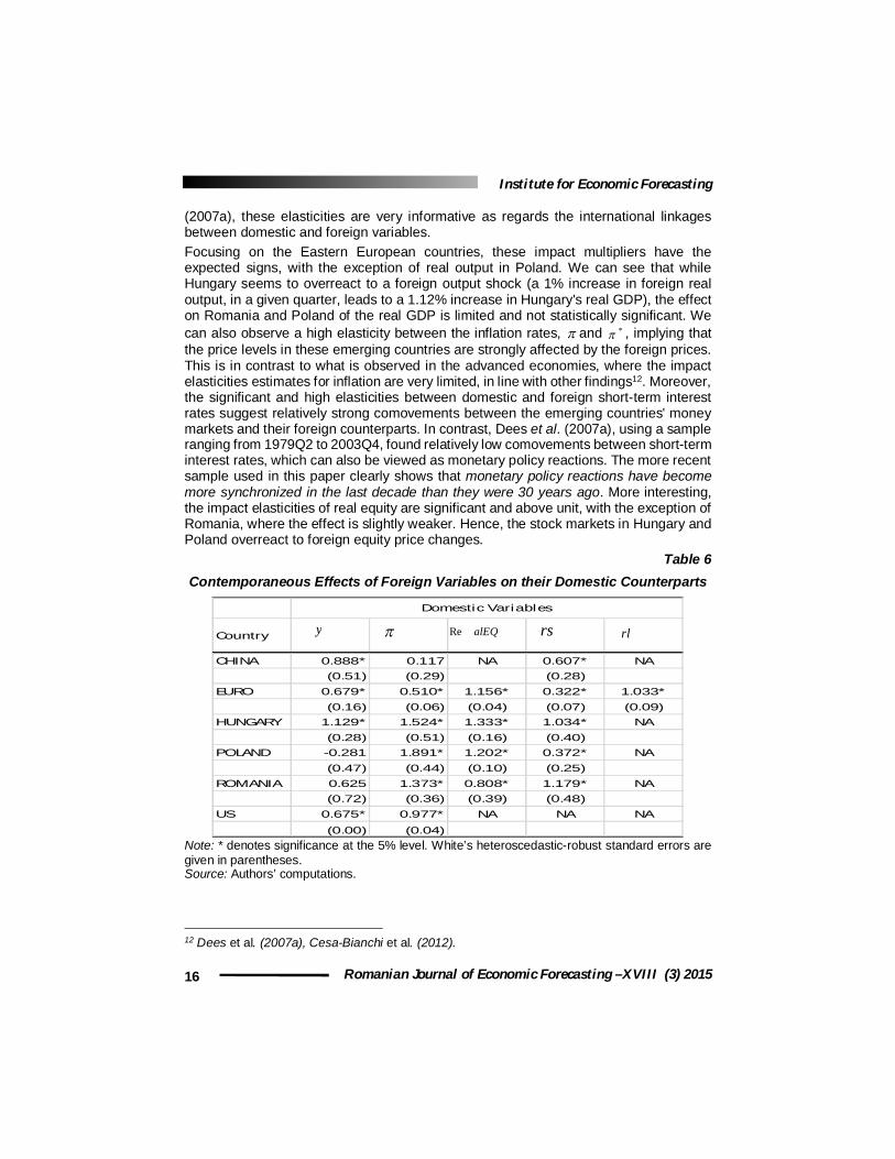
3.5. Contemporaneous Effects of Foreign Variables The contemporaneous effects of foreign variables on their domestic counterparts, the
0i coefficients from equation (9), represent the impact elasticities between foreign and domestic variables, which measure the contemporaneous variation of a domestic variable due to 1% change in its corresponding foreign-specific counterpart. A set of estimates for the focus countries is presented in Table 6. As noted in Dees et al.
CHINA F(1,37) 4.105 3.575 3.938 3.390 NA 0.751 3.910 0.341EURO F(3,33) 2.892 0.469 0.390 0.953 NA 0.948 1.979 0.113HUNGARY F(2,35) 3.267 0.780 0.340 1.095 NA 1.312 0.860 0.324POLAND F(2,35) 3.267 0.051 0.875 0.479 NA 1.438 0.650 0.299ROMANIA F(2,35) 3.267 0.259 0.132 1.639 NA 0.282 1.011 0.945
US F(1,39) 4.091 0.765 0.141 NA 0.772 NA NA NA
Country F test Fcrit_5% *y * *RealEQ *Re alEx *rs *rlop
Institute for Economic Forecasting
Romanian Journal of Economic Forecasting –XVIII (3) 2015 16
(2007a), these elasticities are very informative as regards the international linkages between domestic and foreign variables. Focusing on the Eastern European countries, these impact multipliers have the expected signs, with the exception of real output in Poland. We can see that while Hungary seems to overreact to a foreign output shock (a 1% increase in foreign real output, in a given quarter, leads to a 1.12% increase in Hungary's real GDP), the effect on Romania and Poland of the real GDP is limited and not statistically significant. We can also observe a high elasticity between the inflation rates, and * , implying that the price levels in these emerging countries are strongly affected by the foreign prices. This is in contrast to what is observed in the advanced economies, where the impact elasticities estimates for inflation are very limited, in line with other findings12. Moreover, the significant and high elasticities between domestic and foreign short-term interest rates suggest relatively strong comovements between the emerging countries' money markets and their foreign counterparts. In contrast, Dees et al. (2007a), using a sample ranging from 1979Q2 to 2003Q4, found relatively low comovements between short-term interest rates, which can also be viewed as monetary policy reactions. The more recent sample used in this paper clearly shows that monetary policy reactions have become more synchronized in the last decade than they were 30 years ago. More interesting, the impact elasticities of real equity are significant and above unit, with the exception of Romania, where the effect is slightly weaker. Hence, the stock markets in Hungary and Poland overreact to foreign equity price changes.
Table 6 Contemporaneous Effects of Foreign Variables on their Domestic Counterparts
Note: * denotes significance at the 5% level. White’s heteroscedastic-robust standard errors are given in parentheses. Source: Authors’ computations.
12 Dees et al. (2007a), Cesa-Bianchi et al. (2012).
CHINA 0.888* 0.117 NA 0.607* NA(0.51) (0.29) (0.28)
EURO 0.679* 0.510* 1.156* 0.322* 1.033*(0.16) (0.06) (0.04) (0.07) (0.09)
HUNGARY 1.129* 1.524* 1.333* 1.034* NA(0.28) (0.51) (0.16) (0.40)
POLAND -0.281 1.891* 1.202* 0.372* NA(0.47) (0.44) (0.10) (0.25)
ROMANIA 0.625 1.373* 0.808* 1.179* NA(0.72) (0.36) (0.39) (0.48)
US 0.675* 0.977* NA NA NA
(0.00) (0.04)
Domestic Variables
Country y alEQRe rs rl
Eastern Europe in the World Economy: A Global VAR Analysis
Romanian Journal of Economic Forecasting – XVIII (3) 2015 17
3.6. Serial and Pairwise Cross-Section Correlation of Residuals13 One of the key assumptions underlying the GVAR methodology is that the idiosyncratic shocks of the individual VECMX* models should be “weakly correlated”. Following Dees et al. (2007a), we check this condition by computing the average pairwise cross-section correlations for the residuals associated with the VECMX* models estimated in section 3.3. The presence of the “weakly exogenous” foreign variables, viewed as proxies for common global factors, should capture most of the remaining correlation that exists between country/region specific shocks. The residual interdependencies could reflect policy spillover effects and the situations of contagion. Except for the real exchange rate, these average cross-section correlations are very small and do not depend on the choice of variable or country. The model has successfully captured the cross-section correlations present in level or differenced variables. The high correlations of exchange rates residuals requires further research and does not arise from the simple VARX*(1, 1) structure, as other GVAR models, with a richer structure and estimated over a larger sample, contain the same relatively high correlation for these variables. Due to data limitations, simple VECMX*(1, 1) specifications were chosen to model the endogenous variables in the country-specific models. To test the adequacy of these models, we compute the F statistics for the serial correlation of order 4 in the residuals of the error-correction models. It is encouraging that 133 out of 149 regressions pass the serial correlation test at 5% significance level.
4. Transmission of Shocks in the Global Economy
To investigate the international transmission of shocks and how they affect the economies in Eastern Europe, we analyze the implications of four different shock scenarios: a one standard error negative shock to the U.S. GDP a one standard error negative shock to the U.S. Real Equity Prices a one standard error positive shock to the U.S. interest rates a one standard error negative shock to the Euro Area GDP Besides the three emerging economies from Eastern Europe: Romania, Hungary, Poland, we will also take the Euro Area and Switzerland as benchmarks for developed countries/regions in order to analyze possible asymmetric responses to shocks between the developed and the emerging economies. To this end, we make use of the GIRFs which have the desirable properties of being invariant to the ordering of the variables considering the historical correlations between the innovations of the estimated models. Although the shocks may not be viewed as structural shocks, the GIRFs provide a historically consistent account of the inter-dependencies of the idiosyncratic shocks across countries/regions (Pesaran et al. (2004).
13 The results are presented in Appendix C, available in the online version of the paper.
Institute for Economic Forecasting
Romanian Journal of Economic Forecasting –XVIII (3) 2015 18
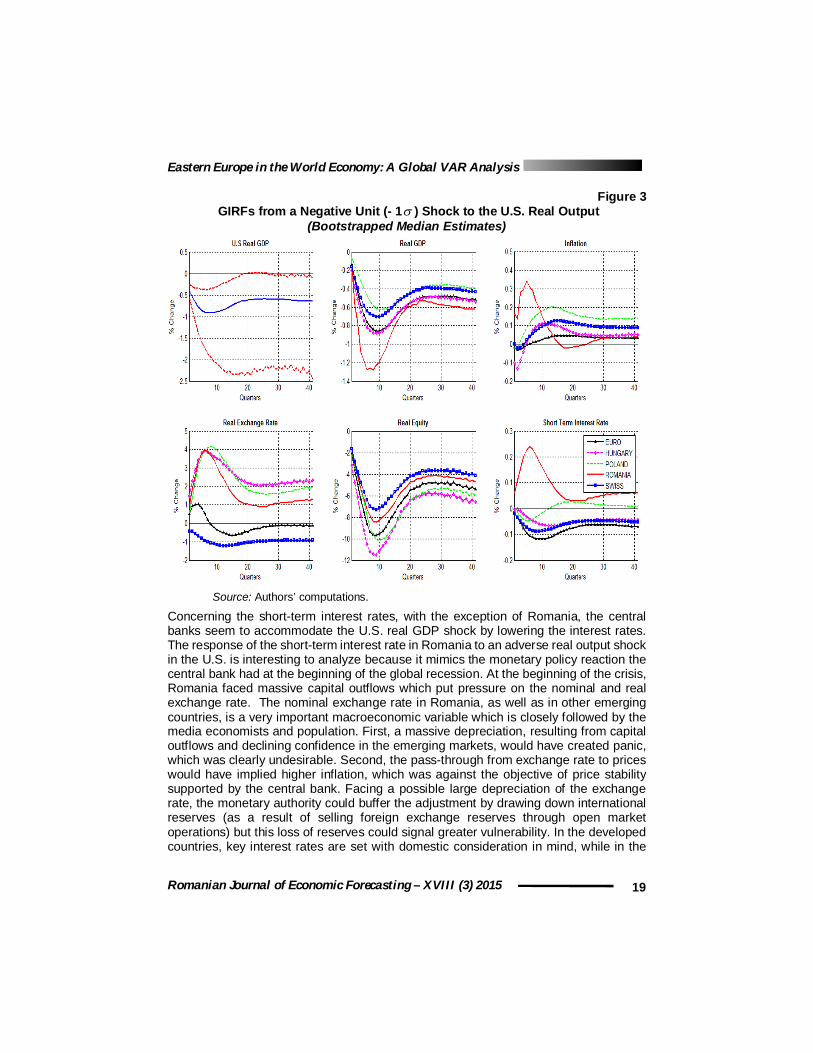
4.1. A Negative Shock to the U.S. GDP Figure 3 reports the GIRFs bootstrapped median estimates (with corresponding 90% confidence bands)14 from one negative standard error shock on the U.S. real output, equivalent to a 0.4% initial decrease in the U.S. real GDP. Over time, the U.S. output appears to decrease, reaching a loss of almost 1% of real GDP in the 6th quarter. The decrease in real GDP is associated with a decrease in inflation, short-term interest rates and equity prices, the last two being significant up to a period of three years. As noted in Dees et al. (2007a), although the shock cannot be interpreted as a structural one, it can be viewed, given the signs of the responses, as a demand shock. The transmission of shock seems to be relatively slow, noticing that outputs in most countries seem to reach their minimum after 2 years. On impact real output is reduced by 35-50% the shock on the U.S. GDP with the exception of Poland (only 14% of the initial U.S. GDP shock), which is relatively less affected by the shock than the other considered countries. Romania, on the other hand, faces the largest and fastest drop in real output, the minimum of 1.3% loss in real output being reached after seven quarters. Over time, the shock propagation increases and gets amplified. The responses of real output become statistically significant after three quarters in Romania and four in Poland, while in the case of Hungary it is significant from the impact. Overall, the 0.4% decrease in the U.S. real output caused a permanent decrease in output by 0.4% in Poland, 0.5% in Hungary and 0.6% in Romania. Given the weight of the U.S. in these emerging countries' trade (around 2%), these results show that other channels are important in the transmission of shocks. As a result of the shock, inflation appears to decrease in all the countries, except for Romania. However, the responses are not statistically significant in none of the countries of focus. The real exchange rate in the developed countries tends to appreciate in the long run, although the response is limited and not statistically significant. Asymmetrically, the real exchange rates in the countries from Eastern Europe suffer a significant depreciation of almost 4%. These asymmetric responses could be interpreted as a “flight to quality”. Financial linkages appear to be another important channel in the transmission of shocks. The equity markets seem to react strongly to the decrease in the U.S. real GDP. Equity prices decrease by around 7-12% in the first two years, almost twice as compared to the U.S. equity prices. This strong response could be another cause of the pronounced decrease in output.
14 We used a sieve bootstrap method with 2000 replications and a 0.9 shrinkage parameter for
the covariance matrix (see Dees et al. (2007b) for a detailed presentation of the bootstrap procedure for the GVAR model).
Eastern Europe in the World Economy: A Global VAR Analysis
Romanian Journal of Economic Forecasting – XVIII (3) 2015 19
Figure 3 GIRFs from a Negative Unit (- 1 ) Shock to the U.S. Real Output
(Bootstrapped Median Estimates)
Source: Authors’ computations.
Concerning the short-term interest rates, with the exception of Romania, the central banks seem to accommodate the U.S. real GDP shock by lowering the interest rates. The response of the short-term interest rate in Romania to an adverse real output shock in the U.S. is interesting to analyze because it mimics the monetary policy reaction the central bank had at the beginning of the global recession. At the beginning of the crisis, Romania faced massive capital outflows which put pressure on the nominal and real exchange rate. The nominal exchange rate in Romania, as well as in other emerging countries, is a very important macroeconomic variable which is closely followed by the media economists and population. First, a massive depreciation, resulting from capital outflows and declining confidence in the emerging markets, would have created panic, which was clearly undesirable. Second, the pass-through from exchange rate to prices would have implied higher inflation, which was against the objective of price stability supported by the central bank. Facing a possible large depreciation of the exchange rate, the monetary authority could buffer the adjustment by drawing down international reserves (as a result of selling foreign exchange reserves through open market operations) but this loss of reserves could signal greater vulnerability. In the developed countries, key interest rates are set with domestic consideration in mind, while in the

Institute for Economic Forecasting
Romanian Journal of Economic Forecasting –XVIII (3) 2015 20
emerging countries they are also used as a stabilization tool for the exchange rate. Considering all the above arguments, it appears that the monetary policy in Romania during the first year of the 2008 crisis was a mix of “fear of floating” and “fear of losing international reserves”, in the sense that the central bank preferred to use the interest rate policy to smooth the exchange rate instead of the other available policies. This reaction15 of the central bank during the recent crisis could have been a way of restoring investor confidence and steeding up capital outflows, and also another cause of the large drop in the real output. However, the above hypothesis requires further consideration. We have also experimented with a structural shock identified by a Cholesky decomposition of the covariance matrix for the U.S model. The results are almost identical to the ones presented in Figure 3, confirming the modest correlations still present in the residuals.
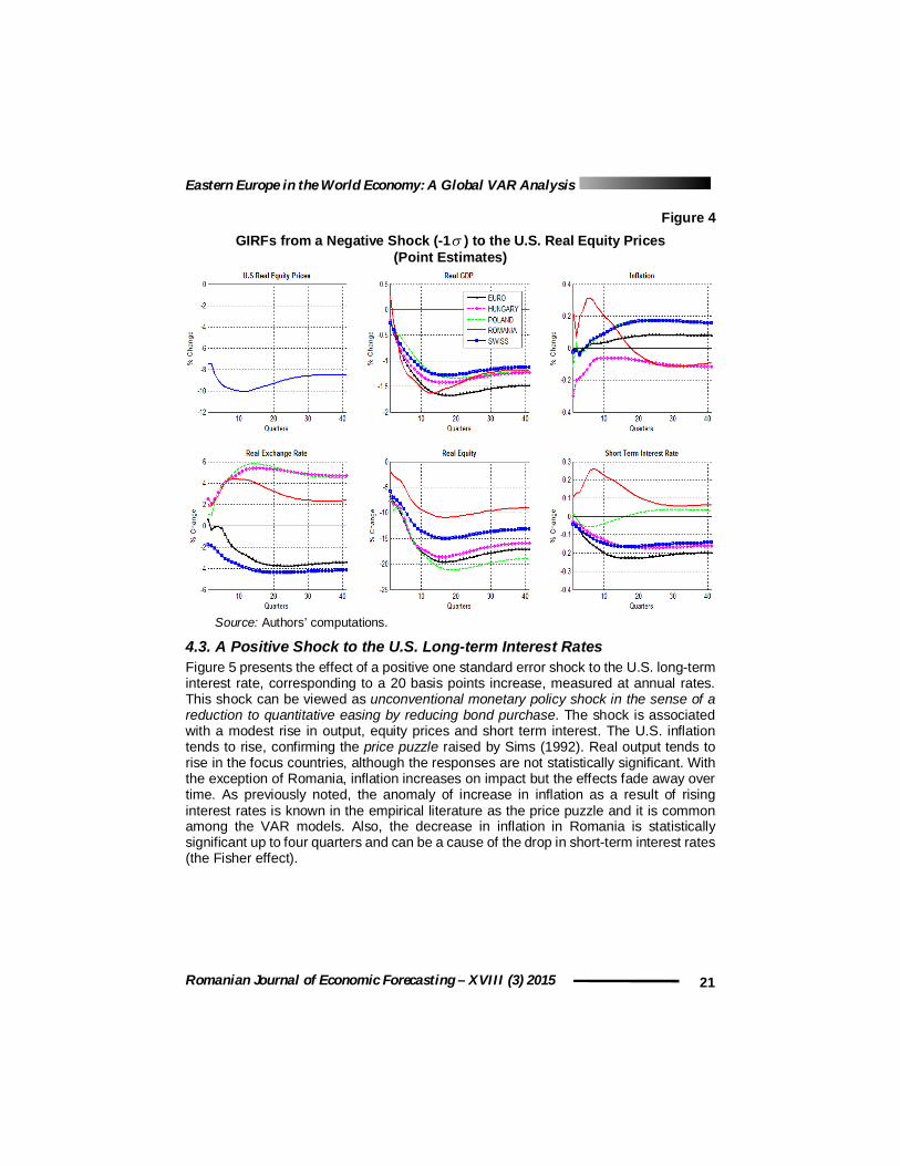
4.2. A Negative Shock to U.S. Equity Prices The point estimates of the GIRFs for one standard error negative shock to the U.S equity prices over a ten year horizon are given in Figure 4. The point estimates were used instead of the bootstrap median estimates due to the rather ragged nature of the last GIRFs in the case of equity shock. This shock corresponds to a 7.4% decrease in the U.S. equity prices on impact, and a decline by 10% after 2 years. The U.S. real GDP declines by 0.4% on impact and by 0.7% on average in the first two years, while inflation and interest rates tend to decrease initially, although the response is limited. The transmission mechanism to the other equity markets seems rather fast and significant. On impact, the equity prices fall by 7.7% in Hungary, 5.6% in Poland, 2% in Romania, while in the other two developed economies the fall is around 6%. Over time, the decrease in equity prices is amplified and, with the exception of the equity market in Romania, the response is stronger as compared to the decrease in the U.S. equity markets. In the case of Poland and Hungary, the overall impact is two times stronger than the decrease in the U.S. equity prices and almost 3 times as compared to the initial shock. This demonstrates that the equity markets in the emerging economies tend to overshoot the U.S. response, thus showing greater volatility as compared to the U.S. counterpart and greater vulnerability to adverse financial shocks. The equity market in Romania seems to be less affected by the equity shock in the U.S. than the other countries of focus. The real output is negatively affected by the equity shock, although to a lesser extent. Similarly to the U.S. real GDP shock, we observe an asymmetric response of the real exchange rates in the emerging countries as compared to the developed economies, noting that the depreciation is even greater in the case of Poland and Hungary. Finally, with the exception of Romania, short-term interest rates and inflation tend to decrease.
15 The National Bank of Romania raised the reference interest rate from 7.5% at the beginning of
2008 to 10.25% in the first quarter of 2009.
Eastern Europe in the World Economy: A Global VAR Analysis
Romanian Journal of Economic Forecasting – XVIII (3) 2015 21
Figure 4 GIRFs from a Negative Shock (-1 ) to the U.S. Real Equity Prices
(Point Estimates)
Source: Authors’ computations.
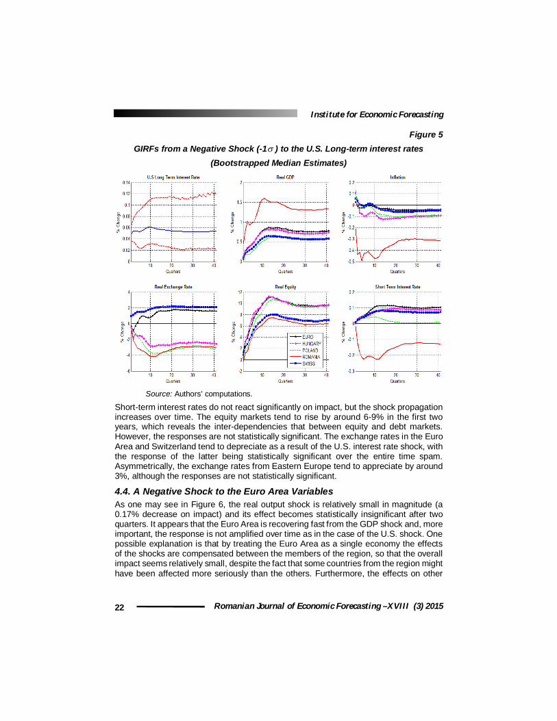
4.3. A Positive Shock to the U.S. Long-term Interest Rates Figure 5 presents the effect of a positive one standard error shock to the U.S. long-term interest rate, corresponding to a 20 basis points increase, measured at annual rates. This shock can be viewed as unconventional monetary policy shock in the sense of a reduction to quantitative easing by reducing bond purchase. The shock is associated with a modest rise in output, equity prices and short term interest. The U.S. inflation tends to rise, confirming the price puzzle raised by Sims (1992). Real output tends to rise in the focus countries, although the responses are not statistically significant. With the exception of Romania, inflation increases on impact but the effects fade away over time. As previously noted, the anomaly of increase in inflation as a result of rising interest rates is known in the empirical literature as the price puzzle and it is common among the VAR models. Also, the decrease in inflation in Romania is statistically significant up to four quarters and can be a cause of the drop in short-term interest rates (the Fisher effect).
Institute for Economic Forecasting
Romanian Journal of Economic Forecasting –XVIII (3) 2015 22
Figure 5 GIRFs from a Negative Shock (-1 ) to the U.S. Long-term interest rates
(Bootstrapped Median Estimates)
Source: Authors’ computations.
Short-term interest rates do not react significantly on impact, but the shock propagation increases over time. The equity markets tend to rise by around 6-9% in the first two years, which reveals the inter-dependencies that between equity and debt markets. However, the responses are not statistically significant. The exchange rates in the Euro Area and Switzerland tend to depreciate as a result of the U.S. interest rate shock, with the response of the latter being statistically significant over the entire time spam. Asymmetrically, the exchange rates from Eastern Europe tend to appreciate by around 3%, although the responses are not statistically significant.
4.4. A Negative Shock to the Euro Area Variables As one may see in Figure 6, the real output shock is relatively small in magnitude (a 0.17% decrease on impact) and its effect becomes statistically insignificant after two quarters. It appears that the Euro Area is recovering fast from the GDP shock and, more important, the response is not amplified over time as in the case of the U.S. shock. One possible explanation is that by treating the Euro Area as a single economy the effects of the shocks are compensated between the members of the region, so that the overall impact seems relatively small, despite the fact that some countries from the region might have been affected more seriously than the others. Furthermore, the effects on other

Eastern Europe in the World Economy: A Global VAR Analysis
Romanian Journal of Economic Forecasting – XVIII (3) 2015 23
variables should be treated with caution. The response of the variables from the countries of interest is very limited and not statistically significant at a 10% level.
Figure 6 GIRF of Euro Area Real GDP from a Negative Shock (-1 ) to the Euro Area Real
GDP (Bootstrapped Median Estimates)
Source: Authors’ computations.
The real GDP in Hungary drops by 0.3% and is significant up to two quarters, while the real exchange rate depreciates by 1.5%. The shock is associated with a decrease in inflation and real equity prices, while the effect on interest rates is mixed. These results seem odd taking into account the large trade shares that these countries have with the Euro Area. It should be emphasized that the U.S. GDP shock that affected the Euro Area and propagated afterwards to the Eastern Europe is not the same as the shock that originated in the Euro Area. These shocks have different characteristics, one of them being the contemporaneous correlations of the errors, which are clearly not identical. A negative one standard error shock to the Euro Area real equity prices corresponds to a decrease by 1.4% on impact and an average of -0.4% in the first year. Similar to the real output shock, the equity market appears to recover rather fast, although the response is not statistically significant. Other markets react similarly to the Euro Area response, with a decrease of almost 1% on impact. The decrease by 0.2% in Poland real output is significant up to two quarters, while the real GDP in Romania and Hungary tends to rise. The shock is associated with a decrease in interest rates and a depreciation of the real exchange rates. Overall, the effects of the Euro Area equity shock are very limited and not statistically significant. As previously pointed, the effects of the shocks originating in the Euro Area may be not very accurate due to the fact that Euro Area was treated as a single economy.
5. Conclusions
This paper investigates the international linkages and the international transmission mechanism of shocks in three emerging economies from Eastern Europe: Romania, Hungary and Poland. In order to capture the complexity of international inter-dependencies between the national economies, the GVAR model developed by Pesaran et al. (2004) is used.
-2,0%
-1,0%
0,0%
1,0%
2,0%
3,0%
0 4 8 12 16 20 24 28 32 36 40
chan
ge
Quarters
Euro Area Real GDP

Institute for Economic Forecasting
Romanian Journal of Economic Forecasting –XVIII (3) 2015 24
The analysis is focused on four shock scenarios, of which three originate in the U.S.: a negative GDP shock, a negative equity shock, a positive long-term interest rate shock, and one in the Euro Area: a negative GDP shock. Generalized impulse-response functions (GIRFs) are used to evaluate the effects of these shocks on the variables from Eastern Europe and a bootstrap procedure is applied in order to determine the significance of these responses. The results of the U.S. real output and equity shocks clearly showed that financial shocks appear to be transmitted much faster than the shock to the real GDP, results in line with the findings of Dess et al. (2007a). Also, the emerging equity markets tend to overshoot the U.S. response, with the overall effect being almost three times higher than the initial U.S. response. The results clearly show a high degree of synchronization of the equity markets. The effects of the U.S. real output shock on the real GDP in the emerging countries is rather small on impact, but the propagation increases over time, normally taking two years before the full impacts are felt. Real GDP in Romania decreases by 1.6%, while real output in Poland seems to be less affected by the U.S. GDP shock as compared to the countries of focus. Taking into account the small trade share that these emerging countries have with the U.S., the responses clearly show the importance of other transmission mechanisms than the trade one, and the importance of second and even third round effects of the shocks originating from the U.S. Regarding the real exchange rates dynamics, an interesting pattern emerges: as a result of the adverse U.S. real output shock, as well as the negative equity shock, the real exchange rates from Eastern Europe react asymmetrically as compared to the response of exchange rates from the developed markets. This asymmetric response between developed and emerging countries real exchange rates could be viewed as a flight to quality as investors seek more stable markets in face of global deteriorating economic conditions. Also, the volatility of exchange rates from Eastern European countries is higher as compared to the counterparts from the other analyzed countries. With the exception of Romania, the monetary authorities appear to accommodate the adverse shocks from the U.S. by lowering the interest rates. The hypothesis proposed to explain the increase in the short-term interest rates in Romania suggests that the central bank could manifest a mix of fear of floating and fear of losing reserves. Compared to the shocks originating from U.S., the shocks from the Euro Area do not get amplified over time. The Euro Area seems to recover rather fast from the shocks and the effects on other variables are very limited. One possible explanation for these responses is that by treating the Euro Area as a single economy the effects of shocks could compensate between its members, so that the overall effect could appear smaller than it actually is.
Acknowledgment
This work was supported by a grant of the Romanian National Authority for Scientific Research, CNCS – UEFISCDI, project number PN-II-ID-PCE-2011-3-1054.
Eastern Europe in the World Economy: A Global VAR Analysis
Romanian Journal of Economic Forecasting – XVIII (3) 2015 25
References
Cesa-Bianchi, A. Pesaran, M.H., Rebucci, A. and Xu, T., 2012. China's emergence in the world economy and business cycles in Latin America. Economia, Journal of the Latin American and Caribbean Economic Association, 12(2), pp.1-75.
Dees, S. di Mauro F. Pesaran, M.H. and Smith, L.V., 2007a. Exploring the international linkages of the euro Area: a global VAR analysis. Journal of Applied Econometrics, 22(1), pp. 1-38.
Dees, S. Holly, S. Pesaran, M.H. and Smith, L.V., 2007b. Long Run Macroeconomic Relations in the Global Economy. Economics: The Open-Access, Open-Assessment E-Journal, 1, 2007-3, pp.1-57.
Harbo, I. Johansen, S. Nielsen, B. and Rahbek, A., 1998. Asymptotic inference on cointegrating rank in partial systems. Journal of Business and Economic Statistics, 16, pp.388–399.
Johansen, S., 1992. Cointegration in Partial Systems and the Efficiency of Single- Equation Analysis. Journal of Econometrics, 52(3), pp.389-402.
Koop .G, Pesaran, M.H. and Potter, S.M., 1996. Impulse response analysis in nonlinear multivariate models. Journal of Econometrics, 74, pp. 119–147.
Park, H. and Fuller, W., 1995. Alternative estimators and unit root tests for the autoregressive process. Journal of Time Series Analysis, 16, pp. 415–429.
Pesaran, M.H, Shin, Y. and Smith, R., 2000. Structural analysis of vector error correction models with exogenous I(1) variables. Journal of Econometrics, 97,pp. 293–343.
Pesaran, M.H. Schuermann, T. and Weiner, S.M., 2004. Modelling regional interdependencies using a global error-correcting macroeconometric model. Journal of Business and Economic Statistics, 22, pp.129–162.
Pesaran, M.H. and Shin, Y., 1996. Cointegration and speed of convergence to equilibrium. Journal of Econometrics, 71(1-2), pp.117-143.
Pesaran, M.H. and Shin, Y., 1998. Generalized impulse response analysis in linear multivariate models. Economics Letters, 58(1), pp.17-29.
Sims, C.A., 1992. Interpreting the Macroeconomic Time Series Facts: The Effects of Monetary Policy. European Economic Review, 36, pp. 975–1000.
Smith, L.V. and Galesi, A., 2011. GVAR Toolbox 1.1 User Guide, CFAP & CIMF, University of Cambridge, Cambridge.
Smith, L.V. and Galesi A., 2012. GVAR Toolbox 2.0.
Sun, Y., Heinz, F.F. and Ho, G., 2013. Cross-Country Linkages in Europe: A Global VAR Analysis. IMF Working Papers 13/194, International Monetary Fund.

Institute for Economic Forecasting
Romanian Journal of Economic Forecasting –XVIII (3) 2015 26
Appendix A - Data Sources
The source for construction of the country specific GDP-PPP weights, global GDP and global Trade is the World Development Indicator database of the World Bank. The data for country-specific imports and exports in millions US dollars was taken from IMF, Direction of Trade Statistics. With the exception of Romania, Hungary and Poland the main source for the data for the variables included in the model is the GVAR data (2011 Vintage) available at: https://sites.google.com/site/gvarmodelling/ data. The real GDP series (2005=100) for the Eastern European countries were collected from IMF International Financial Statistics (IFS). Consistent with the methodology of the GVAR data (2011 Vintage), the time-series for real GDP were first deseasonalized using the Census X12 procedure in Eviews with an additive option. The data for CPI (2005=100), short term interest rate and exchange rates (average) were taken from IMF IFS. In the case of Romania and Hungary, the deposit rate was taken as the short-term interest rate, while in the vase of Poland the money-market interest rate was adopted. For the equity markets, the following indexes were used: BET index in Romania, WIG-20 in Poland and BUX in Hungary. The time series were collected from local stock markets and from http://stooq.com. Finally, the data for long term interest rates were not available for the economies of Eastern Europe.