Module 6: Rotation Loading of a 1D Cantilever Beam 0 …cassenti/AnsysTutorial/Modules_APDL...UCONN...

UCONN ANSYS –Module 6: Rotation Loading of a 1D Cantilever Beam

Module 6: Rotation Loading of a 1D Cantilever Beam

Table of Contents Page Number

Problem Description 2

Theory 3

Geometry 4

Preprocessor 7

Element Type 7

Real Constants and Material Properties 7

Meshing 9

Loads 10

Solution 12

General Postprocessor 12

Results 15

Validation 16

1

MN MXX

Y

Z

0

.383E-03.765E-03

.001148.00153

.001913.002295

.002678.003061

.003443

FEB 27 2012

03:26:57

NODAL SOLUTION

STEP=1

SUB =1

TIME=1

UX (AVG)

RSYS=0

DMX =.003443

SMX =.003443


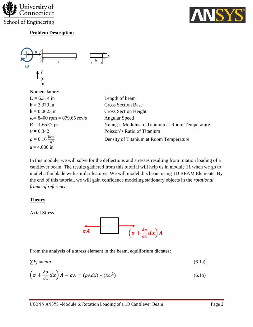
Problem Description

Nomenclature:

L = 6.314 in Length of beam

b = 3.379 in Cross Section Base

h = 0.0623 in Cross Section Height

= 8400 rpm = 879.65 rev/s Angular Speed

E = 1.65E7 psi Young’s Modulus of Titanium at Room Temperature

= 0.342 Poisson’s Ratio of Titanium

= 0.16

Density of Titanium at Room Temperature

a = 4.686 in

In this module, we will solve for the deflections and stresses resulting from rotation loading of a

cantilever beam. The results gathered from this tutorial will help us in module 11 when we go to

model a fan blade with similar features. We will model this beam using 1D BEAM Elements. By

the end of this tutorial, we will gain confidence modeling stationary objects in the rotational

frame of reference.

Theory

Axial Stress

From the analysis of a stress element in the beam, equilibrium dictates:

(6.1a)

(

) (6.1b)

𝝎 y

x

a

𝝈𝑨 (𝝈 𝝏𝝈

𝝏𝒙𝒅𝒙)𝑨


Integrating with respect to x and using the boundary condition we get:

(6.2)

With max stress = 15.87 ksi. Multiplying by Area, we get

Since the max stress is 12.4% the yield stress of Titanium, we are in the linear elastic range of

the stress-strain relationship.

Axial Deflection

Given the relationship:

(6.3)

and

(6.4a)

We get

(6.4b)

Integrating eqn 6.2 with respect to x with the boundary we get

(

)

(6.5)

With maximum deflection


Geometry

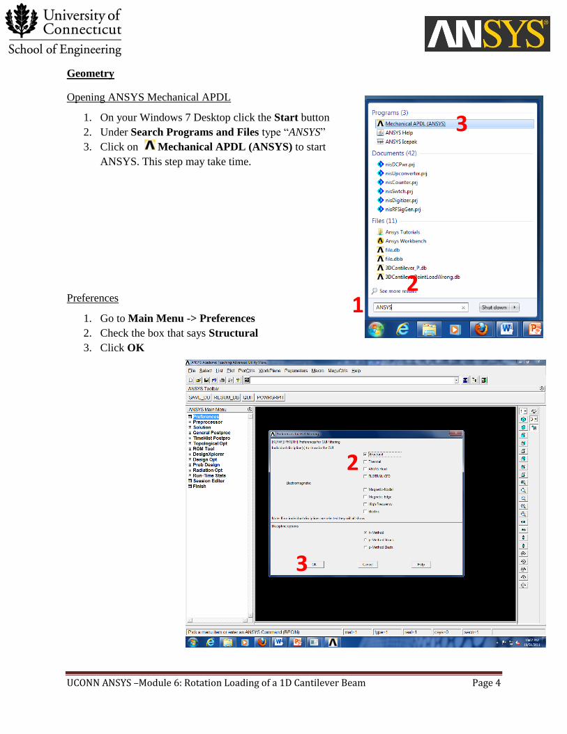
Opening ANSYS Mechanical APDL

1. On your Windows 7 Desktop click the Start button

2. Under Search Programs and Files type “ANSYS”

3. Click on Mechanical APDL (ANSYS) to start

ANSYS. This step may take time.

Preferences

1. Go to Main Menu -> Preferences

2. Check the box that says Structural

3. Click OK

1

2

2

3

3


Keypoints

Since we will be using 1D Elements, our goal is to model the length of the beam.

Go to Main Menu -> Preprocessor -> Modeling -> Create ->Keypoints ->

On Working Plane

1. Click Global Cartesian

2. In the box underneath, write 4.686,0 creating a keypoint at the start of

the beam.

3. Click Apply

4. Repeat Steps 3 and 4 for the point 11,0

5. Click Ok

Let’s check our work.

6. Click the Dynamic Model Mode icon. On the graphics window,

right click and drag the cursor down. You should now be able to see

the two key points you have just created.

7. To get rid of the triad, type /triad,off in Utility Menu -> Command Prompt

8. Go to Utility Menu -> Plot -> Replot

Your graphics window should look as shown:

1

2

8

7


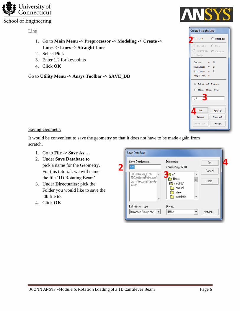
Line

1. Go to Main Menu -> Preprocessor -> Modeling -> Create ->

Lines -> Lines -> Straight Line

2. Select Pick

3. Enter 1,2 for keypoints

4. Click OK

Go to Utility Menu -> Ansys Toolbar -> SAVE_DB

Saving Geometry

It would be convenient to save the geometry so that it does not have to be made again from

scratch.

1. Go to File -> Save As …

2. Under Save Database to

pick a name for the Geometry.

For this tutorial, we will name

the file ‘1D Rotating Beam’

3. Under Directories: pick the

Folder you would like to save the

.db file to.

4. Click OK

4

2

3

2

3

4


Preprocessor

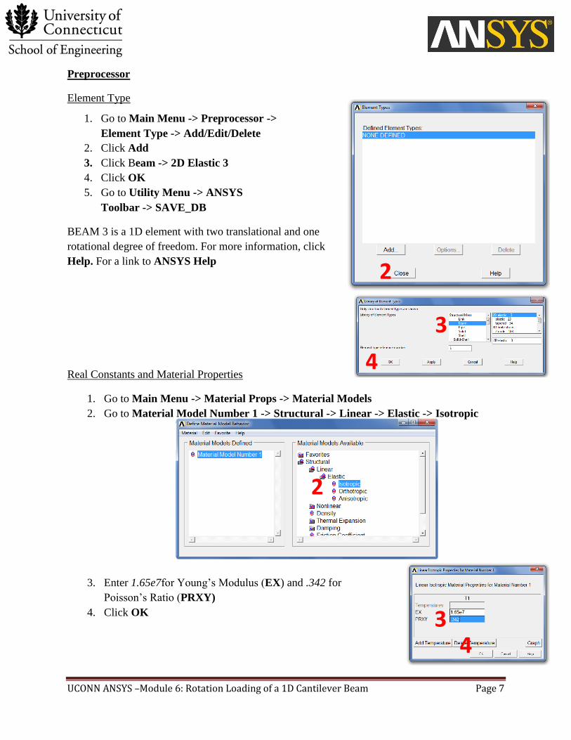
Element Type

1. Go to Main Menu -> Preprocessor ->

Element Type -> Add/Edit/Delete

2. Click Add

3. Click Beam -> 2D Elastic 3

4. Click OK

5. Go to Utility Menu -> ANSYS

Toolbar -> SAVE_DB

BEAM 3 is a 1D element with two translational and one

rotational degree of freedom. For more information, click

Help. For a link to ANSYS Help

Real Constants and Material Properties

1. Go to Main Menu -> Material Props -> Material Models

2. Go to Material Model Number 1 -> Structural -> Linear -> Elastic -> Isotropic

3. Enter 1.65e7for Young’s Modulus (EX) and .342 for

Poisson’s Ratio (PRXY)

4. Click OK

2

3

3

3

4

2

4

3


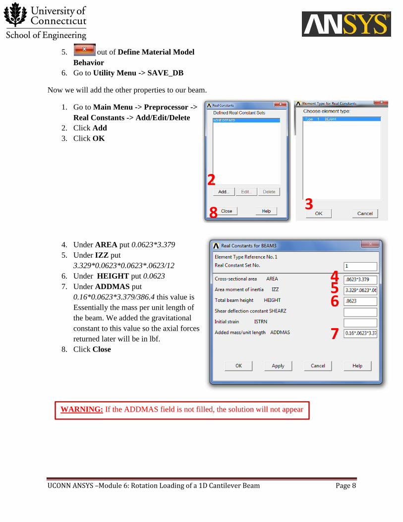
5. out of Define Material Model

Behavior

6. Go to Utility Menu -> SAVE_DB

Now we will add the other properties to our beam.


Real Constants -> Add/Edit/Delete

2. Click Add

3. Click OK

4. Under AREA put 0.0623*3.379

5. Under IZZ put

3.329*0.0623*0.0623*.0623/12

6. Under HEIGHT put 0.0623

7. Under ADDMAS put

0.16*0.0623*3.379/386.4 this value is

Essentially the mass per unit length of

the beam. We added the gravitational

constant to this value so the axial forces

returned later will be in lbf.

8. Click Close

2

3

WARNING: If the ADDMAS field is not filled, the solution will not appear

8

4

5

6

7


Meshing


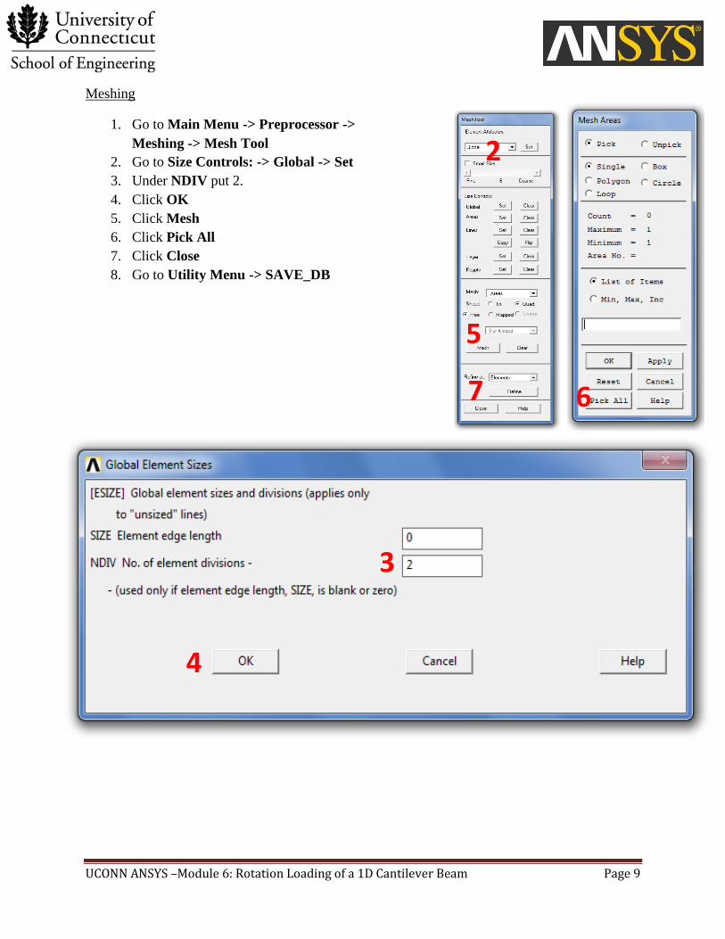
Meshing -> Mesh Tool

2. Go to Size Controls: -> Global -> Set

3. Under NDIV put 2.

4. Click OK

5. Click Mesh

6. Click Pick All

7. Click Close


2

5

56

3

4

7


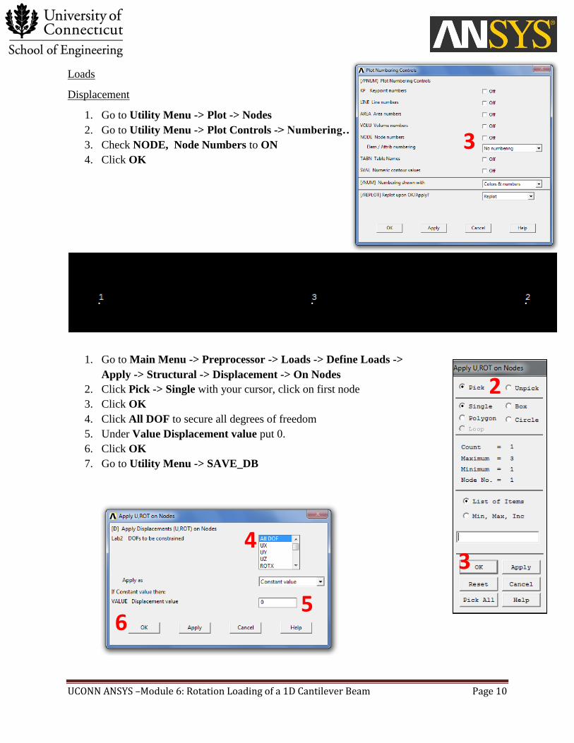
Loads

Displacement

1. Go to Utility Menu -> Plot -> Nodes

2. Go to Utility Menu -> Plot Controls -> Numbering…

3. Check NODE, Node Numbers to ON

4. Click OK

1. Go to Main Menu -> Preprocessor -> Loads -> Define Loads ->

Apply -> Structural -> Displacement -> On Nodes

2. Click Pick -> Single with your cursor, click on first node

3. Click OK

4. Click All DOF to secure all degrees of freedom

5. Under Value Displacement value put 0.

6. Click OK


3

4

2

5

6

4

3


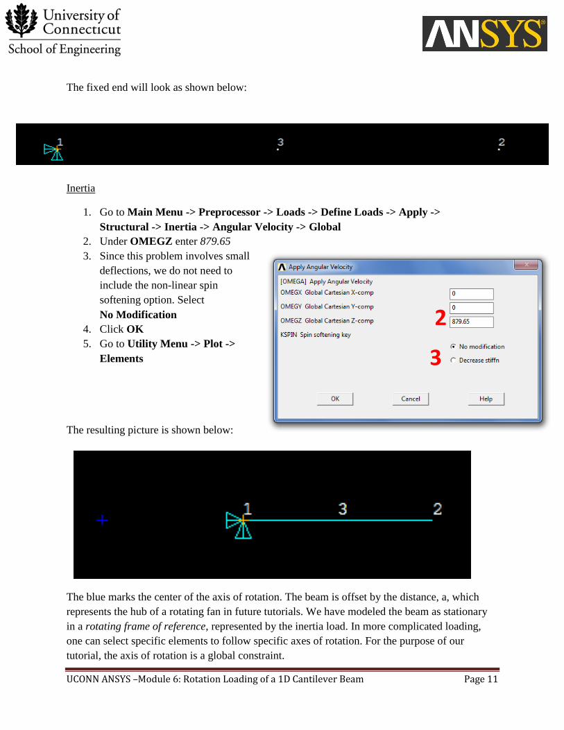
The fixed end will look as shown below:

Inertia

1. Go to Main Menu -> Preprocessor -> Loads -> Define Loads -> Apply ->

Structural -> Inertia -> Angular Velocity -> Global

2. Under OMEGZ enter 879.65

3. Since this problem involves small

deflections, we do not need to

include the non-linear spin

softening option. Select

No Modification

4. Click OK

5. Go to Utility Menu -> Plot ->

Elements

The resulting picture is shown below:

The blue marks the center of the axis of rotation. The beam is offset by the distance, a, which

represents the hub of a rotating fan in future tutorials. We have modeled the beam as stationary

in a rotating frame of reference, represented by the inertia load. In more complicated loading,

one can select specific elements to follow specific axes of rotation. For the purpose of our

tutorial, the axis of rotation is a global constraint.

2

3


Solution

1. Go to Main Menu -> Solution ->Solve -> Current LS (solve). LS stands for Load Step.

This step may take some time depending on mesh size and the speed of your computer

(generally a minute or less).

General Postprocessor

Deflection

1. Go to Main Menu -> General Postprocessor -> Plot Results -> Deformed Shape

2. Select Def + undeformed

3. Click OK

As expected, the beam experiences slight axial

deformation as shown below:

4. Go to Main Menu -> General Postprocessor -> Plot Results -> Contour Plot ->

Nodal Solu -> DOF Solution -> X-Component of displacement -> OK

The following plot should generate:

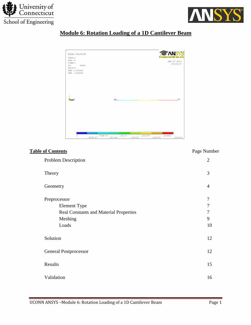
As shown on the contour band, the largest deflection in the beam was calculated as 0.003443in,

perfectly aligning with the theoretical value! For info on plot aesthetics, see module 1.4 page 16.


Axial Stress

Unfortunately, since we are modeling with 1D BEAM elements, we cannot generate plots for

stress. We can however, look up all available force items in a list file organized by node. If we

divide axial force by the cross sectional area of the beam, it should produce the expected axial

stress.

1. Go to Utility Menu -> List -> Results -> Element Solution… ->

All Available Force Items - > OK

The following list file should populate:

The FX column has all of the axial force items of interest. Looking at node 1, if we divide the

value in the table by the cross sectional area of the beam, we get an axial stress of 15.87 ksi, the

exact theoretical value!


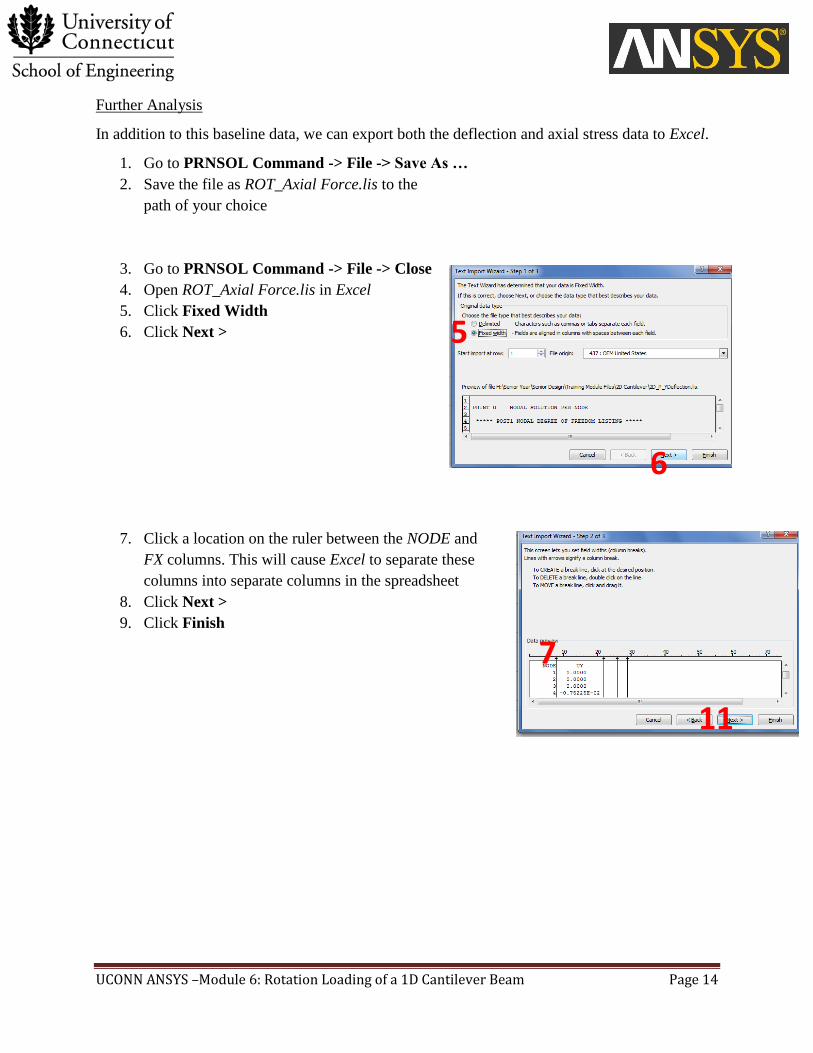
Further Analysis

In addition to this baseline data, we can export both the deflection and axial stress data to Excel.

1. Go to PRNSOL Command -> File -> Save As …

2. Save the file as ROT_Axial Force.lis to the

path of your choice

3. Go to PRNSOL Command -> File -> Close

4. Open ROT_Axial Force.lis in Excel

5. Click Fixed Width

6. Click Next >

7. Click a location on the ruler between the NODE and

FX columns. This will cause Excel to separate these

columns into separate columns in the spreadsheet

8. Click Next >

9. Click Finish

5

6

7

11


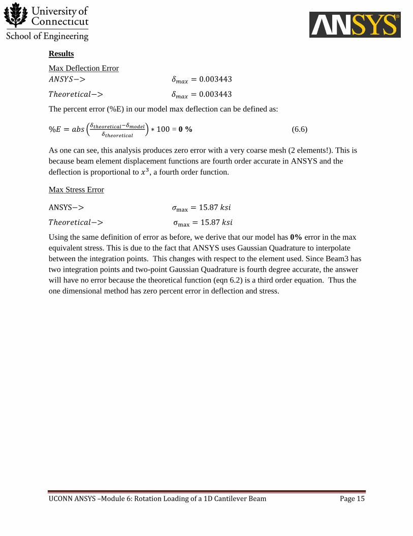
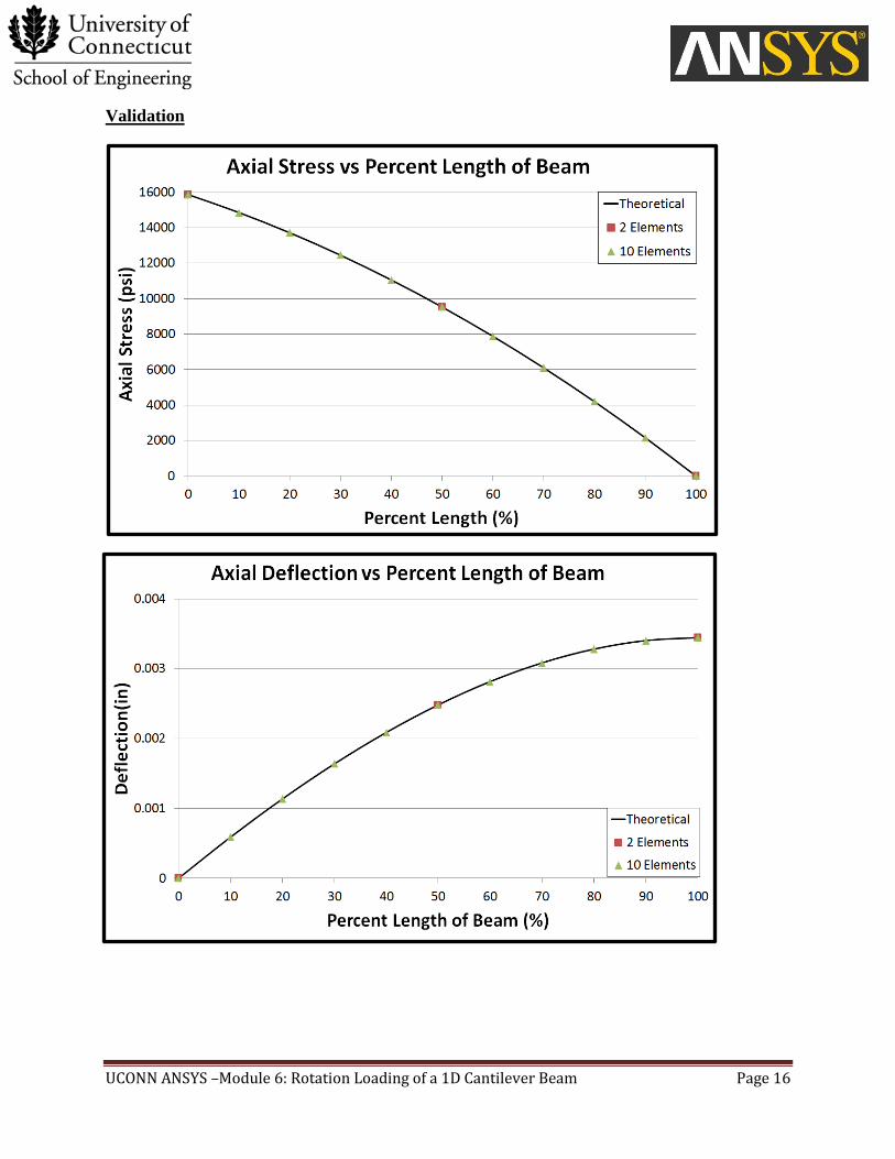
Results

Max Deflection Error

The percent error (%E) in our model max deflection can be defined as:

(

) = 0 % (6.6)

As one can see, this analysis produces zero error with a very coarse mesh (2 elements!). This is

because beam element displacement functions are fourth order accurate in ANSYS and the

deflection is proportional to , a fourth order function.

Max Stress Error

Using the same definition of error as before, we derive that our model has 0% error in the max

equivalent stress. This is due to the fact that ANSYS uses Gaussian Quadrature to interpolate

between the integration points. This changes with respect to the element used. Since Beam3 has

two integration points and two-point Gaussian Quadrature is fourth degree accurate, the answer

will have no error because the theoretical function (eqn 6.2) is a third order equation. Thus the

one dimensional method has zero percent error in deflection and stress.


Validation

Module 6: Rotation Loading of a 1D Cantilever Beam 0 …cassenti/AnsysTutorial/Modules_APDL...UCONN...

Documents

Transcript of Module 6: Rotation Loading of a 1D Cantilever Beam 0 …cassenti/AnsysTutorial/Modules_APDL...UCONN...