Module 5

Classical True ScoreTheory and Reliability

Any phenomenon we decide to “measure” in psychology, whether it isa physical or mental characteristic, will inevitably contain some error.

For example, you can step on the same scale three consecutive times to weighyourself and get three slightly different readings. To deal with this, youmight take the average of the three weight measures as the best guess of yourcurrent weight. In most field settings, however, we do not have the luxuryof administering our measurement instrument multiple times. We get oneshot at it and we had better obtain the most accurate estimate possible withthat one administration. Therefore, if we have at least some measurementerror estimating a physical characteristic such as weight, a construct thateveryone pretty much agrees on, imagine how much error is associated witha controversial psychological phenomenon we might want to measuresuch as intelligence. With classical psychometric true score theory, we canstop “imagining” how much error there is in our measurements and startestimating it.

Classical true score theory states that our observed score (X) is equal tothe sum of our true score, or true underlying ability (T), plus the measure-ment error (E) associated with estimating our observed scores, or

X = T + E

Several assumptions are made about the relationship among these threecomponents. These assumptions are discussed in detail in texts such as Allen

69

05-Shultz.qxd 6/4/2004 6:01 PM Page 69

and Yen (1979) and Crocker and Algina (1986), so we will not cover themhere. Briefly, however, the “true score” is the score we would obtain if we wereto take the average score for an infinite number of test administrations. Ofcourse, in practice, one cannot administer a test an infinite number of times,and as noted previously, the vast majority of the time we get only one chance.Therefore, we use reliability coefficients to estimate both true and errorvariance associated with our observed test scores. Theoretically speaking, ourreliability estimate is the ratio of the true variance to the total variance:

where rxx is the reliability, σ2true is the true score variance, σ2

total is the totalscore variance, and σ2

error is the error variance. Of course, we will never beable to directly estimate the true score and its variance; hence, this particu-lar formula serves merely as a heuristic for understanding the components ofreliability. In the following discussion, we will outline several options forestimating test reliability in practice.

Estimating Reliability in Practice

Right about now you are probably saying to yourself, “Okay, that’s the the-oretical stuff that my textbook talked about, but how do I actually computea reliability estimate when I need to?” Most of the time, we compute aPearson product moment correlation coefficient (correlation coefficient forshort) or some other appropriate estimate (e.g., a Spearman correlation if wehave ordinal data) to estimate the reliability of our measurement scale.

Before we can calculate our reliability estimate, however, we have todecide what type of measurement error we want to focus on. For example,if we want to account for changes in test scores due to time, we calculate thecorrelation coefficient between a test given at time 1 and the same test givenat some later point (i.e., test-retest reliability). Therefore, once we knowwhat source of error we want to focus on, we will know what type of relia-bility coefficient we are dealing with and thus which correlation coefficientto compute to estimate our reliability.

Looking at the first column of Table 5.1, you will notice three differentsources of measurement error that we can estimate with different types ofreliability estimates. Notice, however, that one source of measurement error,

70——Reliability, Validity, and Test Bias

rxx =σ 2

true =σ 2

true

σ 2total σ2

true + σ2error

05-Shultz.qxd 6/4/2004 6:01 PM Page 70

content sampling, appears twice. Each of these sources can be considered tobe tapping into the issue of how consistent our measures are. The first sourceof error, change in examinees, estimates how consistently our examineesrespond from one occasion to another. The next two, content sampling,estimate how consistent items are across test versions or within a given test.Finally, we may estimate the consistency of raters’ judgments of examineesor test items.

Classical True Score Theory and Reliability——71

Reliability Reliability Source of Error Coefficient Estimate Statistic

Change in Stability Test/retest r12

examinees

Content Equivalence Alternate forms rxx'

sampling

Content sampling Internal consistency Split-half rx1x2

Alpha α

Inter-rater Rater consistency Inter-rater kappa

Table 5.1 Sources of Error and Their Associated Reliability and Statistics

The second column in Table 5.1 lists the type of reliability coefficient touse when we estimate a given source of measurement error. For example,with changes in examinees our reliability coefficient is an estimate of stabil-ity or consistency of examinees’ responses over time. With the first form ofcontent sampling measurement error (i.e., row 2 in Table 5.1), we are mea-suring the equivalence or consistency of different forms of a test. However,with the second form of content sampling measurement error (i.e., row 3 inTable 5.1), we are measuring what is commonly referred to as the internalconsistency of test items. That is, do all the items in a single test seem to betapping the same underlying construct? Finally, when we estimate inter-ratersources of measurement error, our reliability coefficient is one of rater con-sistency. That is, do raters seem to be rating the target in a consistent man-ner, whether the target is the test itself or individuals taking the test, such asjob applicants during an employment interview?

The third column in Table 5.1 presents the name of the reliability estimatewe would use to determine the respective sources of measurement error. Forexample, if we wanted to estimate sources of measurement error associated

05-Shultz.qxd 6/4/2004 6:01 PM Page 71

with changes in examinees over time, we would compute a test-retestreliability estimate. Alternatively, if we wanted to examine the first form ofcontent sampling, we would compute what is commonly known as alternateforms reliability (also referred to as parallel forms reliability). However, forthe second form of content sampling, we do not need to have a second formof the test. We would instead compute either a split-half reliability coeffi-cient or an alpha reliability coefficient to estimate the internal consistency ofa single test. Finally, for estimating sources of error associated with raters,we would compute an inter-rater reliability estimate.

You may remember that in Module 2 we discussed the importance of thecorrelation coefficient. Why is it so important? As you can see in the lastcolumn of Table 5.1, the correlation coefficient is used to compute mostforms of reliability estimates. The only difference among the different corre-lation coefficients is the variables used and the interpretation of the resultingcorrelation. For example, with a test-retest reliability estimate, we wouldcompute the correlation coefficient between individuals’ scores on a giventest taken at time 1 and those same individuals’ scores on the same test takenat a later date. The higher the correlation coefficient, the more reliable thetest or, conversely, the less error attributable to changes in the examineesover time. Of course, many things can affect the test-retest estimate of relia-bility. One is the nature of the construct being assessed. For example, whenwe are measuring enduring psychological traits, such as most forms ofpersonality, there should be little change over time. However, if we weremeasuring transitory psychological states, such as fear, then we wouldexpect to see more change from the first to the second testing. As a result,our test-retest reliability estimates tend to be lower when we are measuringtransitory psychological states rather than enduring psychological traits.

In addition, the length of time between testing administrations can affectour estimate of stability. For instance, if we are measuring a cognitive skillsuch as fluency in a foreign language, and there is a long time period betweentesting sessions, an individual may be able to practice that language andacquire additional fluency in that language between testing sessions. As aresult, individuals will score consistently higher on the second occasion.However, differences in scores from time 1 to time 2 will be interpreted asinstability in subjects (i.e., a lot of measurement error) and not learning. Onthe other hand, if we make the duration between testing sessions too short,examinees may remember their previous responses. There may also be fatigueeffects associated with the test-retest if the retest is immediate. So how longshould the interval between testing sessions be? Unfortunately, there is nohard-and-fast rule. The key is to make sure that the duration is long enoughnot to fatigue the examinees or allow them to remember their answers, but

72——Reliability, Validity, and Test Bias

05-Shultz.qxd 6/4/2004 6:01 PM Page 72

not so long that changes may take place (e.g., learning, psychologicaltraumas) that could impact our estimate of reliability. Of course, one wayto deal with the possibility of subjects remembering their answers from time1 to time 2 is to use two different forms of the test.

With alternate forms reliability, we administer examinees one form of thetest and then at a later date give them a second form of the test. Because wedo not have to worry about the individuals remembering their answers, theintervening time between testing sessions does not need to be as long as withtest-retest reliability estimates. In fact, the two testing sessions may even occuron the same day. From a practical standpoint, this may be ideal, in that exam-inees may be unwilling or simply fail to return for a second testing session. Asyou have probably surmised, the biggest disadvantage of the alternate formsmethod is that you need to have two versions of the test. It is hard enough todevelop one psychometrically sound form of a test, now you have to createtwo. Is it possible to just look at content sampling within a single test?

With split-half and alpha reliability estimates, we need only one version ofthe test. To estimate split-half reliability, we correlate one half of the test withthe other half of the test. If we simply correlate the first half with the secondhalf, however, we may have spuriously low reliability estimates due to fatigueeffects. In addition, many cognitive ability tests are spiral in nature, meaningthey start out easy and get harder as you go along. As a result, correlatingthe first half of the test with the second half of the test may be misleading.Therefore, to estimate split-half reliability, most researchers correlate scoreson the odd-numbered items with scores on the even-numbered items. As youmight have guessed by now, we are, in a sense, computing a correlation ononly half of our test. Does that in and of itself result in a lower reliability esti-mate? In fact, it does. Therefore, whenever a split-half reliability estimate iscalculated, one should also use the Spearman-Brown prophecy formula tocorrect for the fact that we are cutting the test in half. (Note: We demonstratean alternate use of the formula in Case Study 5.2.)

where rXX'nis the Spearman-Brown corrected split-half reliability estimate;

n is the factor by which we want to increase the test, which in this casewould be 2 (because we are, in a sense, doubling the test back to its originallength); and rXX′ is the original split-half reliability estimate. Because n isalways equal to 2 when correcting our split-half reliability estimate, ourformula can be simplified to

Classical True Score Theory and Reliability——73

rXX′n=

nrXX′

1 + (n − 1)rXX′

05-Shultz.qxd 6/4/2004 6:01 PM Page 73

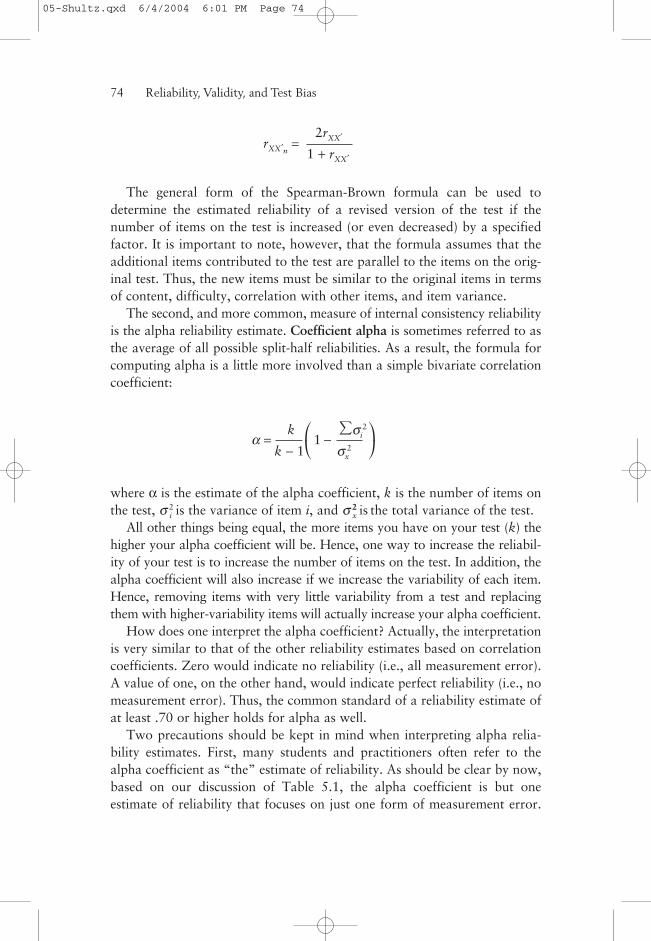
The general form of the Spearman-Brown formula can be used todetermine the estimated reliability of a revised version of the test if thenumber of items on the test is increased (or even decreased) by a specifiedfactor. It is important to note, however, that the formula assumes that theadditional items contributed to the test are parallel to the items on the orig-inal test. Thus, the new items must be similar to the original items in termsof content, difficulty, correlation with other items, and item variance.

The second, and more common, measure of internal consistency reliabilityis the alpha reliability estimate. Coefficient alpha is sometimes referred to asthe average of all possible split-half reliabilities. As a result, the formula forcomputing alpha is a little more involved than a simple bivariate correlationcoefficient:

where α is the estimate of the alpha coefficient, k is the number of items onthe test, σ 2

i is the variance of item i, and σ 22x is the total variance of the test.

All other things being equal, the more items you have on your test (k) thehigher your alpha coefficient will be. Hence, one way to increase the reliabil-ity of your test is to increase the number of items on the test. In addition, thealpha coefficient will also increase if we increase the variability of each item.Hence, removing items with very little variability from a test and replacingthem with higher-variability items will actually increase your alpha coefficient.

How does one interpret the alpha coefficient? Actually, the interpretationis very similar to that of the other reliability estimates based on correlationcoefficients. Zero would indicate no reliability (i.e., all measurement error).A value of one, on the other hand, would indicate perfect reliability (i.e., nomeasurement error). Thus, the common standard of a reliability estimate ofat least .70 or higher holds for alpha as well.

Two precautions should be kept in mind when interpreting alpha relia-bility estimates. First, many students and practitioners often refer to thealpha coefficient as “the” estimate of reliability. As should be clear by now,based on our discussion of Table 5.1, the alpha coefficient is but oneestimate of reliability that focuses on just one form of measurement error.

74——Reliability, Validity, and Test Bias

rXX′n=

2rXX′

1 + rXX′

α =k

1 −

∑σi

2

k − 1 σx2

⎛⎝

⎞⎠

05-Shultz.qxd 6/4/2004 6:01 PM Page 74

Therefore, if you are interested in other forms of measurement error (such asstability over time), you will need to compute additional reliability estimates.Second, as Cortina (1993) and Schmitt (1996) pointed out, one common mis-conception of alpha among naive researchers is that the alpha coefficient isan indication of the unidimensionality of a test. As pointed out previously,if you have a large enough set of items, you will have a high alpha coeffi-cient, but this does not mean your test is unidimensional. The measurementof job satisfaction can serve as a good example of this phenomenon. Mostjob satisfaction scales measure several different facets of job satisfaction,such as satisfaction with one’s job, supervisor, pay, advancement opportu-nities, and so on. However, the scales can also be combined to create anoverall job satisfaction score. Clearly, this overall job satisfaction score is notunidimensional. Because the overall score is typically based on a largenumber of items, however, the overall scale’s alpha coefficient will be large.As a result, it is important for researchers to remember that an alpha coeffi-cient only measures one form of measurement error and is an indication ofinternal consistency, not unidimensionality.

Finally, to estimate inter-rater agreement, a statistic such as Cohen’skappa can be used. To compute kappa, sometimes referred to as scorer reli-ability, you would need to set up a cross-tabulation of ratings given by raters,similar to a chi-square contingency table. For example, you might have agroup of parents, both the mother and the father (your two raters), rate theirchildren on the children’s temperament (e.g., 1 = easygoing, 2 = anxious,3 = neither). You would want to then determine if the parents agree in termsof their respective perceptions (and ratings) of their children’s temperaments.To compute the kappa statistic, you would need to set up a 2(raters) ×3(temperament rating) contingency table of the parents’ ratings. Then youwould compute the kappa statistic as follows:

where k is the kappa statistic, Oa is the observed count of agreement (typi-cally reported in the diagonal of the table), Ea is the expected count of agree-ment, and N is the total number of respondent pairs. Thus, Cohen’s kapparepresents the proportion of agreement among raters after chance agreementhas been factored out. In this case, zero represents chance ratings, while ascore of one represents perfect agreement. (Note: Exercise 5.3 provides datafor computing Cohen’s kappa.)

Classical True Score Theory and Reliability——75

k =(Oa − Ea)

(N − Ea)

05-Shultz.qxd 6/4/2004 6:01 PM Page 75

As with many statistics, however, kappa has not been without its critics(e.g., Maclure & Willett, 1987). One criticism is that kappa is not a good esti-mate of effect size. Although it will give a pretty good estimate of whether theobserved ratings are significantly different from chance (an inferential statis-tic), using kappa as an estimate of the actual degree of agreement (i.e., as aneffect size estimate) should be done cautiously, as the statistic assumes theraters are independent. In our preceding example, it is highly unlikely that theparents will provide independent ratings. Thus, when it can be reasonablyassumed that raters are not independent, you would be better off using otherestimates of rater agreement, such as the intraclass correlation coefficient.

Thus, we see there are many forms of reliability, each of which estimates adifferent source of measurement error. In general, immediate test-retest relia-bility and split-half reliability tend to provide upper-bound estimates of reliabi-lity. That is, they tend to provide higher estimates, on average, than otherforms of reliability. Coefficient alpha and long-term test-retest tend toprovide somewhat lower estimates, on average, while alternate formsreliability, both short and long term, tends to provide lower-bound esti-mates. Why present this information here? These general trends are impor-tant both for interpreting your obtained reliability coefficients and for usingyour reliability estimates for other purposes, such as determining the stan-dard error of measurement.

What Do We Do With the ReliabilityEstimates Now That We Have Them?

You are probably asking yourself, “Now that we have an estimate of relia-bility, what do we do with it?” First, we will need to report our reliabilityestimate(s) in any manuscripts (e.g., technical manuals, conference papers,and articles) that we write. Second, if we have followed sound basic testconstruction principles, someone who scores high on our test is likely to behigher on the underlying trait than someone who scores low on our test.Often times, this general ranking is all we are really looking for; who is“highest” on a given measure. However, if we want to know how mucherror is associated with a given test score (such as when we set standards orcutoff scores), we can use our reliability estimate to calculate the standarderror of measurement, or SEM (of course, we would also need to knowthe sample standard deviation for the measure). Thus, computing the SEMallows us to build a confidence interval around our observed score so thatwe can estimate (with a certain level of confidence) someone’s underlyingtrue score,

76——Reliability, Validity, and Test Bias

05-Shultz.qxd 6/4/2004 6:01 PM Page 76

where Sx is the sample standard deviation and rxx is the reliability estimate.

EXAMPLE: X = 100, Sx = 10, rxx = .71

95% CI = X ± 1.96*SEM = 100 ± 1.96*(5.38)= 100 ± 10.54 = 89.46 ≤ T ≤ 110.54

where X is our test score, 1.96 is the critical z value associated with the 95%confidence interval, SEM is the standard error of measurement value, andT is our estimated underlying true score value.

You can see from the preceding formula that, as our test becomes morereliable, our confidence interval becomes narrower. For example, if weincrease the reliability of our test to .80, the SEM in the previous examplebecomes 4.47 and thus the 95% confidence interval narrows to 91.24 ≤ T ≤108.76. We could even reverse the formula and figure out how reliable ourtest needs to be if we want a certain width confidence interval for a test witha given standard deviation. For example, if we want to be 95% confidentthat a given true score is within 5 points (SEM = 2.5, plus or minus in eitherdirection) of someone’s observed score, then we would have to have a testwith a reliability of .9375:

Concluding Comments

There will always be some degree of error when we try to measure some-thing. Physical characteristics, however, tend to have less measurement errorthan psychological phenomena. Therefore, it is critical that we accuratelyestimate the amount of error associated with any measure, in particular, psy-chological measures. To estimate the measurement error, we have to firstdecide what form of error we are most interested in estimating. Once we do

Classical True Score Theory and Reliability——77

SEM = 10√1 − .71 = 10 (.5385) = 5.38

SEM = Sx

√1− rxx , becomes 1 −

[SEM

]2

= 1 −

[2.5

]2

= 1 − .0625 = .9375Sx 10

SEM = Sx

√1 − rxx

05-Shultz.qxd 6/4/2004 6:01 PM Page 77

that, we can choose an appropriate reliability estimate (see Table 5.1) toestimate the reliability. We can then use the reliability estimate to build con-fidence intervals around our observed scores to estimate the underlying truescores. In doing so, we will have much more confidence in the interpretationof our measurement instruments.

Practical Questions

1. How much can we shorten an existing measure and still maintain adequatereliability? (See Case Study 5.2.)

2. What are the different sources of error that can be assessed with classical reli-ability analysis?

3. Does it matter which reliability estimate we put into the standard error ofmeasurement formula?

4. Are some reliability estimates generally higher (or lower) than others? Thatis, does one tend to serve as an upper- (or lower-) bound reliabilityestimate?

5. How is Cohen’s kappa estimate of reliability different from the other formsof reliability?

6. Why are some authors (e.g., Cortina, 1993; Schmitt, 1996) cautious aboutthe interpretation of coefficient alpha?

Case Studies

CASE STUDY 5.1: DON’TFORGET TO REVERSE SCORE

It didn’t make sense. It just didn’t. How could the reliability be solow? Chad scratched his head and thought. Chad had agreed to helpanalyze the data from his graduate advisor’s most recent study.Although entering the data into a computer database had not beenexciting, it had been relatively easy. Once he had entered eachresearch participant’s responses, he spot-checked a few cases to ensureaccuracy. He then conducted frequency analyses on each variable toensure that there were no out-of-bounds responders. In fact, he’dfound two cases in which he had incorrectly entered the data. He

78——Reliability, Validity, and Test Bias

05-Shultz.qxd 6/4/2004 6:01 PM Page 78

could tell, because items that were responded to on a five-pointLikert-type rating scale had reported scores of 12 and 35, respectively.Sure enough, he’d just made a typo when entering the data. Everythingelse looked fine.

Or so he thought, until he decided to examine the reliability of one ofthe scales. Chad’s advisor, Dr. John Colman, was primarily interestedin troubled adolescents, and over the last several years had investigatedadolescent attitudes toward alcoholic beverages. The same measure ofadolescent attitudes toward alcohol was routinely used in this research.Respondents indicated on a scale of 1–5 how strongly they agreed witheach of the 12 items. Internal consistency reliability estimates for thescale were consistently good, typically around .80. However, not thistime, apparently. In computing the reliability estimate for the data he’djust entered, Chad found that alpha was estimated to be –.39.

Chad couldn’t remember ever hearing of a negative internal consis-tency reliability estimate. In addition, he couldn’t explain why thescale would have such a different reliability on this sample than it hadwith the many samples his advisor had previously used. His firstthought was that he might have entered the data incorrectly—but heknew he hadn’t. After all, he’d checked the data carefully to ensurethat the computer data file matched exactly what was on the originalsurveys. So what could be the problem?

In examining the item-total correlations for each item on the scale,Chad noticed that several items correlated negatively with a compositeof the remaining items. Chad grabbed the original survey and reexam-ined the 12 items that comprised the adolescent attitudes toward alco-hol scale. Each item certainly seemed to measure the intended construct.Chad was about to give up and go report the problem to his advisorwhen he noticed something. Although each of the 12 items measuredattitudes toward alcohol, agreement to eight of the items would beindicative of acceptance of alcohol use. In contrast, agreement to theother four items would be indicative of a rejection of alcohol use. Thatwas it. He’d correctly entered the data from the surveys into thecomputer data file, but had forgotten to recode the reverse-codeditems. Because his advisor wanted high scores to be indicative of anacceptance of the use of alcohol, Chad decided he’d recode the fourreverse-coded items. To do this, he used the recode command of hisstatistics program to recode all responses of “5” into “1,” “4” into

Classical True Score Theory and Reliability——79

05-Shultz.qxd 6/4/2004 6:01 PM Page 79

“2,” “2” into “4,” and “1” into “5.” He did this for each of the fourreverse-coded items. Holding his breath, he again computed the alpha.This time, the reliability estimate was α = .79, and all of the item-totalcorrelations were positive. Satisfied that he’d been able to resolve theproblem on his own, Chad made a mental note to always recode theappropriate items once the entire data file had been completed.

Questions to Ponder

1. In terms of Table 5.1, what type of reliability coefficient did Chadestimate? What source of error is being estimated?

2. Did Chad make the right interpretation of his negative reliability esti-mate? What else might cause a negative reliability estimate?

3. In practice, how does one know which items to recode and which tokeep the same?

4. Both positively and negatively worded items are frequently included ontests. Assuming you recode the negatively worded items before you runyour reliability analysis, will the inclusion of negatively worded itemsaffect the test’s internal consistency reliability estimate?

CASE STUDY 5.2: LENGTHENING ANDSHORTENING PSYCHOLOGICAL SCALES

Sheila was frustrated. Although she was happy with both the topic andthe constructs she had chosen to examine in her senior honors thesis,she had hit several roadblocks in determining what measures to use toassess each variable in her proposed study. Now that she had finallyidentified useful measures to include in her survey, she was concernedthat her response rate would suffer because of the rather impressivelength of the survey. Reasoning that the sample she hoped to use wasunlikely to spend more than a few minutes voluntarily responding to asurvey, Sheila considered her options. First, she could eliminate one ormore variables. This would make her study simpler and would havethe added benefit of reducing the length of the survey. Sheila rejectedthis option, however, because she felt each variable she had identifiedwas necessary to adequately address her research questions. Second,she considered just mailing the survey to a larger number of people inorder to get an adequate number to respond to the lengthy survey.Sheila quickly rejected this option as well. She certainly didn’t wantto pay for the additional copying and mailing costs. She was also

80——Reliability, Validity, and Test Bias

05-Shultz.qxd 6/4/2004 6:01 PM Page 80

concerned that a lengthy survey would further reduce the possibility ofobtaining a sample that was representative of the population. Perhapsthose individuals who would not respond to a long survey would bevery different from the actual respondents.

Suddenly a grin spread across Sheila’s face. “Couldn’t I shortenthe survey by reducing the number of items used to assess some ofthe variables?” she thought. Some of the scales she had selected tomeasure variables were relatively short, while scales to measure othervariables were quite long. Some of the scales were publisher-ownedmeasures and thus copyrighted. Others were nonproprietary scalesboth created and used by researchers. Recognizing the reluctance ofpublishers to allow unnecessary changes to their scales, Sheila consid-ered the nonproprietary measures. The scale intended to assess opti-mism was not only nonproprietary but also very long: 66 items. Ascale assessing dogmatism was also nonproprietary and, at 50 items,also seemed long. Sheila quickly decided that these would be goodscales to target for reduction of the number of items.

In class, Sheila had learned that the Spearman-Brown prophecy formulacould be used to estimate the reliability of a scale if the scale wasdoubled in length. Her instructor also explained that the same formulacould be used for either increasing or decreasing the number of items bya certain factor. Sheila knew from her research that the typical internalconsistency reliability finding for her optimism scale was .85, andfor the dogmatism scale it was .90. Because she wanted to reduce thenumber of items administered for each scale, she knew the resultingreliability estimates would be lower. But how much lower? Sheila con-sidered reducing the number of items in both scales by one half. Becauseshe was reducing the number of items, the number of times she wasincreasing the scale was equal to one half, or .5. She used this informa-tion to compute the Spearman-Brown reliability estimate as follows:

Classical True Score Theory and Reliability——81

rXX′n

=nrXX′

1 + (n − 1)rXX′

=.5(.85)

1 + (.5 − 1).85

= .74

Optimism Test

rXX′n=

nrXX′

1 + (n − 1)rXX′

=.5(.90)

1 + (.5 − 1).90

= .82

Dogmatism Test

05-Shultz.qxd 6/4/2004 6:01 PM Page 81

In considering these results, Sheila thought she’d be satisfied with aninternal consistency reliability estimate of .82 for the dogmatismscale, but was concerned that too much error would be included inestimates of optimism if the internal consistency reliability estimatewere merely .74.

Undeterred, Sheila decided to estimate the reliability if only one thirdof the optimism items were removed. If one third of the items weredropped, two thirds (or .67) of the original items would remain.Therefore, the Spearman-Brown prophecy estimate could be computedas follows:

Sheila decided this reliability would be acceptable for her study. Inorder to complete her work, Sheila randomly selected 25 (50%) ofthe items from the dogmatism scale, and 44 (67%) of the items fromthe optimism scale. She was confident that although her survey formwas now shorter, the reliability of the individual variables would beacceptable.

Questions to Ponder

1. In terms of Table 5.1, what type of reliability coefficient did Sheila esti-mate? What source of error is being estimated?

2. Should Sheila have randomly selected which items to keep and whichto delete? What other options did she have?

3. How else might Sheila maintain her reliability levels yet still maintain(or increase) the number of usable responses she obtains?

4. Why do you think Sheila is using .80 as her lower acceptable bound forreliability?

82——Reliability, Validity, and Test Bias

Optimism Test

rXX′n

=nrXX′

1 + (n − 1)rXX′

= .67(.85)1 + (.67 − 1).85

= .79

05-Shultz.qxd 6/7/2004 2:25 PM Page 82

Exercises

EXERCISE 5.1: COMPUTING TEST-RETEST,ALPHA, AND PARALLEL FORMS

RELIABILITY VIA COMPUTER

OBJECTIVE: To practice calculating different types of reliability.

Using the data set “Reliability.sav” (see the variable list in AppendixB), perform the reliability analyses outlined below. The scales providedhere include a depression scale (14 items, V1–V14), a life satisfactionscale (10 items, V15–V24), a reasons-a-person-retired scale (10 items,V25–V34), a scale with regard to good things about retirement (8 items,V35–V42), and a scale with regard to bad things about retirement(6 items, V43–V48). For your assignment (be sure to do an ocularanalysis of all items first, checking for outliers, missing data, etc.,before jumping into the reliability analyses):

1. Perform alpha, split-half, and parallel forms reliability analyses foreach of the five scales. How do the three different types of reliabilitycompare for each scale listed above? Is one form of reliability moreappropriate than another? Discuss for each scale. (Note: You may wishto put your results in table form for easy comparison.)

2. Using alpha reliability, with item and scale information, what itemsshould be included in the final versions of each scale in order to max-imize the alpha reliability for that scale? (Note: You will need toexamine the item-total correlations. In addition, once an item isremoved, you will need to repeat the process until a final scale isdecided upon.)

3. For the life satisfaction and depression scales, determine if the alphareliabilities are different for men and women (SEX). If yes, any guesseswhy? (Note: This requires using the “split file” option in SPSS or com-parable options in other statistics programs.)

4. Based on Cortina (1993), what additional analyses could youconduct to evaluate the reliabilities of each of the scales? (You mayperform these analyses if you wish, but it is not required for thisassignment.)

Classical True Score Theory and Reliability——83

05-Shultz.qxd 6/4/2004 6:01 PM Page 83

EXERCISE 5.2: EXAMINING THE EFFECTSOF THE SPEARMAN-BROWN PROPHECY FORMULA

OBJECTIVE: To practice using the Spearman-Brown prophecy formulafor estimating reliability levels.

Using the Spearman-Brown prophecy formula provided in Case Study5.2, estimate Sheila’s reliability for the dogmatism scale if she usedonly one third of the number of original items. Is this an “acceptablelevel” of reliability? Why or why not?

EXERCISE 5.3: ESTIMATING AGREEMENTCOEFFICIENTS (COHEN’S KAPPA)

OBJECTIVE: To practice calculating Cohen’s kappa estimate of rateragreement.

Assume you wanted to determine the degree of inter-rater agreementbetween two forensic psychologists who were each rating 100 poten-tial parolees in terms of their potential for committing additional vio-lent crimes. In general, sociopaths are more likely to commit additionalviolent crimes than are depressed or normal individuals. Therefore,each psychologist rated each of the 100 potential parolees on a scaleof 1–3 in terms of their primary personality category (1 = sociopath,2 = depressed, 3 = normal). The following results were obtained:

Using the data in the preceding table and the formula for kappapresented in the module overview, determine the level of agreementbetween the raters.

84——Reliability, Validity, and Test Bias

Forensic Psychologist A

Forensic Personality 1 Personality 2 Personality 3Psychologist B Personality 1 44 5 1

Personality 2 7 20 3Personality 3 9 5 6

05-Shultz.qxd 6/7/2004 2:24 PM Page 84

Internet Web Site References

5.1. http://trochim.human.cornell.edu/kb/reliable.htm

This Web page presents the beginning of the chapter on reliability from Dr. WilliamM. Trochim’s electronic textbook.

5.2. http://trochim.human.cornell.edu/tutorial/levell/mazeintr.htm

This Web page provides a 10-item quiz on reliability, along with a rationale for thecorrect answer to each item.

5.3. http://www.statsoftinc.com/textbook/streliab.html

This Web page presents the beginning of the chapter on reliability from Statsoft,Inc.’s electronic textbook.

5.4. http://www.ruf.rice.edu/~lane/stat_sim/reliability_reg/

This Web page presents a simulation of the effects of the reliability of X and Y ona number of components of regression analysis.

5.5. http://www.unl.edu/BIACO/workshops/reliability%20folder/sld001.htm

This Web page is the start page of a slide presentation by the Buros Institute forAssessment Consultation and Outreach (BIACO) titled “Consistency in Scoring(Reliability) Workshop.”

5.6. http://chiron.valdosta.edu/mawhatley/3900/reliablec.htm

This Web page provides a 30-item reliability quiz. Responses are scored immediately.Note: Because of the overlap between the concepts presented in Modules 6–8, manyof the links listed under a particular module in this section are likely to presentadditional information relevant to the other modules.

Further Readings

Cortina, J. M. (1993). What is coefficient alpha? An examination of theory andapplications. Journal of Applied Psychology, 78, 98–104.

Maclure, M., & Willett, W. C. (1987). Misinterpretation and misuse of the kappastatistic. American Journal of Epidemiology, 126, 161–169.

Schmidt, F. L., & Hunter, J. E. (1996). Measurement error in psychologicalresearch: Lessons from 26 research scenarios. Psychological Methods, 1,199–223.

Schmitt, N. (1996). Uses and abuses of coefficient alpha. Psychological Assessment,8, 350–353.

Traub, R. E. (1994). Reliability for the social sciences: Theory and application.Thousand Oaks, CA: Sage.

Classical True Score Theory and Reliability——85

05-Shultz.qxd 6/4/2004 6:01 PM Page 85

05-Shultz.qxd 6/4/2004 6:01 PM Page 86