What you will learn in this Module:

482 s e c t i o n 9 B e h i n d t h e D e m a n d C u r v e : C o n s u m e r C h o i c e

• The meaning of consumersurplus and its relationship tothe demand curve

• The meaning of producersurplus and its relationship tothe supply curve

Module 49Consumer andProducer SurplusThere is a lively market in second-hand college textbooks. At the end of each term,some students who took a course decide that the money they can make by selling theirused books is worth more to them than keeping the books. And some students who aretaking the course next term prefer to buy a somewhat battered but less expensive usedtextbook rather than pay full price for a new one.

Textbook publishers and authors are not happy about these transactions becausethey cut into sales of new books. But both the students who sell used books and thosewho buy them clearly benefit from the existence of the market. That is why many col-lege bookstores facilitate their trade, buying used textbooks and selling them alongsidethe new books.

But can we put a number on what used textbook buyers and sellers gain from thesetransactions? Can we answer the question “How much do the buyers and sellers of text-books gain from the existence of the used-book market?”

Yes, we can. In this module we will see how to measure benefits, such as those tobuyers of used textbooks, from being able to purchase a good—known as consumer sur-plus. And we will see that there is a corresponding measure, producer surplus, of the bene-fits sellers receive from being able to sell a good.

The concepts of consumer surplus and producer surplus are useful for analyzinga wide variety of economic issues. They let us calculate how much benefit produc-ers and consumers receive from the existence of a market. They also allow us to cal-culate how the welfare of consumers and producers is affected by changes inmarket prices. Such calculations play a crucial role in evaluating many economicpolicies.

What information do we need to calculate consumer and producer surplus? Surpris-ingly, all we need are the demand and supply curves for a good. That is, the supply anddemand model isn’t just a model of how a competitive market works—it’s also a modelof how much consumers and producers gain from participating in that market. So ourfirst step will be to learn how consumer and producer surplus can be derived from thedemand and supply curves. We will then see how these concepts can be applied to ac-tual economic issues.

Consumer Surplus and the Demand Curve First-year college students are often surprised by the prices of the textbooks requiredfor their classes. The College Board estimates that in 2006-2007 students at four-yearschools spent, on average, $942 for books and supplies. But at the end of the semes-ter, students might again be surprised to find out that they can sell back at leastsome of the textbooks they used for the semester for a percentage of the purchaseprice (offsetting some of the cost of textbooks). The ability to purchase used text-books at the start of the semester and to sell back used textbooks at the end of the se-mester is beneficial to students on a budget. In fact, the market for used textbooks isa big business in terms of dollars and cents—approximately $1.9 billion in 2004–2005. This market provides a convenient starting point for us to develop the con-cepts of consumer and producer surplus. We’ll use the concepts of consumer andproducer surplus to understand exactly how buyers and sellers benefit from a com-petitive market and how big those benefits are. In addition, these concepts assist inthe analysis of what happens when competitive markets don’t work well or there isinterference in the market.

So let’s begin by looking at the market for used textbooks, starting with the buyers.The key point, as we’ll see in a minute, is that the demand curve is derived from theirtastes or preferences—and that those same preferences also determine how much theygain from the opportunity to buy used books.

Willingness to Pay and the Demand CurveA used book is not as good as a new book—it will be battered and coffee-stained, mayinclude someone else’s highlighting, and may not be completely up to date. Howmuch this bothers you depends on your preferences. Some potential buyers wouldprefer to buy the used book even if it is only slightly cheaper than a new one, whileothers would buy the used book only if it is considerably cheaper. Let’s define a po-tential buyer’s willingness to pay as the maximum price at which he or she wouldbuy a good, in this case a used textbook. An individual won’t buy the good if it costsmore than this amount but is eager to do so if it costs less. If the price is just equal toan individual’s willingness to pay, he or she is indifferent between buying and notbuying. For the sake of simplicity, we’ll assume that the individual buys the good inthis case.

The table in Figure 49.1 on the next page shows five potential buyers of a used book that costs $100 new, listed in order of their willingness to pay. At one extreme is Aleisha, who will buy a second-hand book even if the price is as high as $59. Brad is less willing to have a used book and will buy one only if the price is $45 or less. Claudia is willing to pay only $35 and Darren, only $25. Edwina, who really doesn’t like the idea of a used book, will buy one only if it costs no morethan $10.

How many of these five students will actually buy a used book? It depends on theprice. If the price of a used book is $55, only Aleisha buys one; if the price is $40,Aleisha and Brad both buy used books, and so on. So the information in the table canbe used to construct the demand schedule for used textbooks.

We can use this demand schedule to derive the market demand curve shown in Fig-ure 49.1. Because we are considering only a small number of consumers, this curvedoesn’t look like the smooth demand curves we have seen previously, for markets thatcontained hundreds or thousands of consumers. This demand curve is step-shaped,with alternating horizontal and vertical segments. Each horizontal segment—eachstep—corresponds to one potential buyer’s willingness to pay. However, we’ll seeshortly that for the analysis of consumer surplus it doesn’t matter whether the demandcurve is step-shaped, as in this figure, or whether there are many consumers, makingthe curve smooth.

m o d u l e 4 9 C o n s u m e r a n d P ro d u c e r S u r p l u s 483

Section 9 Behind the Demand Curve: Consum

er Choice

A consumer’s willingness to pay for agood is the maximum price at which he orshe would buy that good.

Willingness to Pay and Consumer Surplus Suppose that the campus bookstore makes used textbooks available at a price of $30.In that case Aleisha, Brad, and Claudia will buy books. Do they gain from their pur-chases, and if so, how much?

The answer, shown in Table 49.1, is that each student who purchases a book doesachieve a net gain but that the amount of the gain differs among students.

Aleisha would have been willing to pay $59, so her net gain is $59 − $30 = $29. Bradwould have been willing to pay $45, so his net gain is $45 − $30 = $15. Claudia would

484 s e c t i o n 9 B e h i n d t h e D e m a n d C u r v e : C o n s u m e r C h o i c e

543210

Aleisha

Brad

Claudia

Darren

D

Edwina

$59

45

35

10

25

Price ofbook

Quantity of books

Aleisha

Brad

Claudia

Darren

Edwina

Willingnessto pay

Potentialbuyers

$59

45

35

25

10

The Demand Curve for Used Textbooksf i g u r e 49.1

With only five potential consumers in this market, thedemand curve is step-shaped. Each step represents oneconsumer, and its height indicates that consumer’s will-ingness to pay—the maximum price at which each willbuy a used textbook—as indicated in the table. Aleishahas the highest willingness to pay at $59, Brad has the

next highest at $45, and so on down to Edwina with thelowest willingness to pay at $10. At a price of $59, thequantity demanded is one (Aleisha); at a price of $45,the quantity demanded is two (Aleisha and Brad); and soon until you reach a price of $10, at which all five stu-dents are willing to purchase a book.

Consumer Surplus When the Price of a Used Textbook Is $30

Potential Individual consumer surplus buyer Willingness to pay Price paid = Willingness to pay − Price paid

Aleisha $59 $30 $29

Brad 45 30 15

Claudia 35 30 5

Darren 25 — —

Edwina 10 — —

All buyers Total consumer surplus = $49

t a b l e 49.1

have been willing to pay $35, so her net gain is $35 − $30 = $5. Darren and Edwina, how-ever, won’t be willing to buy a used book at a price of $30, so they neither gain nor lose.

The net gain that a buyer achieves from the purchase of a good is called that buyer’sindividual consumer surplus. What we learn from this example is that whenever abuyer pays a price less than his or her willingness to pay, the buyer achieves some indi-vidual consumer surplus.

The sum of the individual consumer surpluses achieved by all the buyers of a good isknown as the total consumer surplus achieved in the market. In Table 49.1, the totalconsumer surplus is the sum of the individual consumer surpluses achieved by Aleisha,Brad, and Claudia: $29 + $15 + $5 = $49.

Economists often use the term consumer surplus to refer to both individual and totalconsumer surplus. We will follow this practice; it will always be clear in context whether weare referring to the consumer surplus achieved by an individual or by all buyers.

Total consumer surplus can be represented graphically. Figure 49.2 reproduces thedemand curve from Figure 49.1. Each step in that demand curve is one book wide andrepresents one consumer. For example, the height of Aleisha’s step is $59, her willing-ness to pay. This step forms the top of a rectangle, with $30—the price she actually paysfor a book—forming the bottom. The area of Aleisha’s rectangle, ($59 − $30) × 1 = $29,is her consumer surplus from purchasing one book at $30. So the individual consumersurplus Aleisha gains is the area of the dark blue rectangle shown in Figure 49.2.

In addition to Aleisha, Brad and Claudia will also each buy a book when the price is$30. Like Aleisha, they benefit from their purchases, though not as much, because theyeach have a lower willingness to pay. Figure 49.2 also shows the consumer surplusgained by Brad and Claudia; again, this can be measured by the areas of the appropriaterectangles. Darren and Edwina, because they do not buy books at a price of $30, receiveno consumer surplus.

The total consumer surplus achieved in this market is just the sum of the individualconsumer surpluses received by Aleisha, Brad, and Claudia. So total consumer surplus isequal to the combined area of the three rectangles—the entire shaded area in Figure 49.2.Another way to say this is that total consumer surplus is equal to the area below the de-mand curve but above the price.

m o d u l e 4 9 C o n s u m e r a n d P ro d u c e r S u r p l u s 485

Section 9 Behind the Demand Curve: Consum

er Choice

f i g u r e 49.2Consumer Surplus in theUsed-Textbook MarketAt a price of $30, Aleisha, Brad, and Claudiaeach buy a book but Darren and Edwina donot. Aleisha, Brad, and Claudia get individualconsumer surpluses equal to the differencebetween their willingness to pay and the price,illustrated by the areas of the shaded rectan-gles. Both Darren and Edwina have a willing-ness to pay less than $30, so they areunwilling to buy a book in this market; theyreceive zero consumer surplus. The total con-sumer surplus is given by the entire shadedarea—the sum of the individual consumersurpluses of Aleisha, Brad, and Claudia—equal to $29 + $15 + $5 = $49.

543210

Aleisha

Brad

Claudia

Darren

D

Edwina

$59

45

35

30

10

25

Price ofbook

Quantity of books

Price

Brad’s consumer surplus:$45 − $30 = $15

Aleisha’s consumer surplus:$59 − $30 = $29

Claudia’s consumer surplus:$35 − $30 = $5

Individual consumer surplus is the net gain to an individual buyer from thepurchase of a good. It is equal to thedifference between the buyer’s willingness to pay and the price paid.

Total consumer surplus is the sum of the individual consumer surpluses of all the buyers of a good in a market.

The term consumer surplus is often used to refer to both individual and to total consumer surplus.

This is worth repeating as a general principle: The total consumer surplus generated bypurchases of a good at a given price is equal to the area below the demand curve but above thatprice. The same principle applies regardless of the number of consumers.

When we consider large markets, this graphical representation becomes particu-larly helpful. Consider, for example, the sales of personal computers to millions of po-tential buyers. Each potential buyer has a maximum price that he or she is willing topay. With so many potential buyers, the demand curve will be smooth, like the oneshown in Figure 49.3.

486 s e c t i o n 9 B e h i n d t h e D e m a n d C u r v e : C o n s u m e r C h o i c e

f i g u r e 49.3Consumer SurplusThe demand curve for computers is smooth be-cause there are many potential buyers. At aprice of $1,500, 1 million computers are de-manded. The consumer surplus at this price isequal to the shaded area: the area below thedemand curve but above the price. This is thetotal net gain to consumers generated frombuying and consuming computers when theprice is $1,500.

1 million0

Price ofcomputer

Quantity of computers

D

$1,500

Consumer surplus

Price

Suppose that at a price of $1,500, a total of 1 million computers are purchased. Howmuch do consumers gain from being able to buy those 1 million computers? We couldanswer that question by calculating the individual consumer surplus of each buyer andthen adding these numbers up to arrive at a total. But it is much easier just to look atFigure 49.3 and use the fact that total consumer surplus is equal to the shaded areabelow the demand curve but above the price.

How Changing Prices Affect Consumer Surplus It is often important to know how price changes affect consumer surplus. For example,we may want to know the harm to consumers from a frost in Florida that drives up or-ange prices or consumers’ gain from the introduction of fish farming that makessalmon steaks less expensive. The same approach we have used to derive consumer sur-plus can be used to answer questions about how changes in prices affect consumers.

Let’s return to the example of the market for used textbooks. Suppose that thebookstore decided to sell used textbooks for $20 instead of $30. By how much wouldthis fall in price increase consumer surplus?

The answer is illustrated in Figure 49.4. As shown in the figure, there are two partsto the increase in consumer surplus. The first part, shaded dark blue, is the gain ofthose who would have bought books even at the higher price of $30. Each of the stu-dents who would have bought books at $30—Aleisha, Brad, and Claudia—now pays $10less, and therefore each gains $10 in consumer surplus from the fall in price to $20. Sois

tock

phot

o

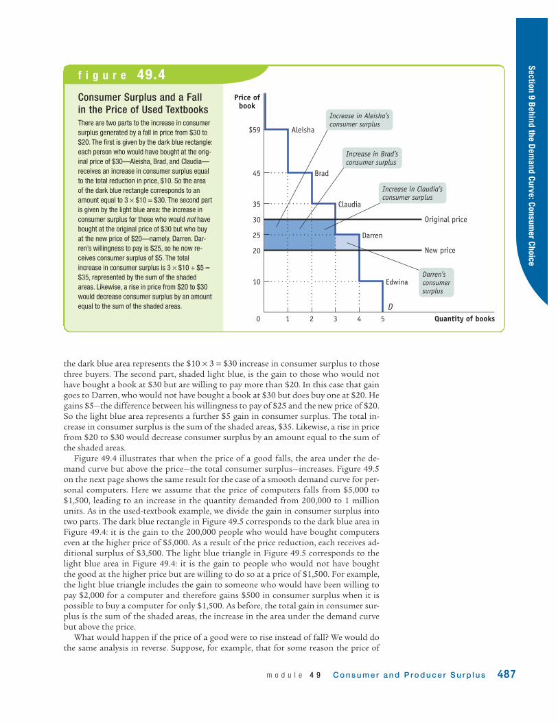
the dark blue area represents the $10 × 3 = $30 increase in consumer surplus to thosethree buyers. The second part, shaded light blue, is the gain to those who would nothave bought a book at $30 but are willing to pay more than $20. In this case that gaingoes to Darren, who would not have bought a book at $30 but does buy one at $20. Hegains $5—the difference between his willingness to pay of $25 and the new price of $20.So the light blue area represents a further $5 gain in consumer surplus. The total in-crease in consumer surplus is the sum of the shaded areas, $35. Likewise, a rise in pricefrom $20 to $30 would decrease consumer surplus by an amount equal to the sum ofthe shaded areas.

Figure 49.4 illustrates that when the price of a good falls, the area under the de-mand curve but above the price—the total consumer surplus—increases. Figure 49.5on the next page shows the same result for the case of a smooth demand curve for per-sonal computers. Here we assume that the price of computers falls from $5,000 to$1,500, leading to an increase in the quantity demanded from 200,000 to 1 millionunits. As in the used-textbook example, we divide the gain in consumer surplus intotwo parts. The dark blue rectangle in Figure 49.5 corresponds to the dark blue area inFigure 49.4: it is the gain to the 200,000 people who would have bought computerseven at the higher price of $5,000. As a result of the price reduction, each receives ad-ditional surplus of $3,500. The light blue triangle in Figure 49.5 corresponds to thelight blue area in Figure 49.4: it is the gain to people who would not have bought the good at the higher price but are willing to do so at a price of $1,500. For example,the light blue triangle includes the gain to someone who would have been willing topay $2,000 for a computer and therefore gains $500 in consumer surplus when it ispossible to buy a computer for only $1,500. As before, the total gain in consumer sur-plus is the sum of the shaded areas, the increase in the area under the demand curvebut above the price.

What would happen if the price of a good were to rise instead of fall? We would dothe same analysis in reverse. Suppose, for example, that for some reason the price of

m o d u l e 4 9 C o n s u m e r a n d P ro d u c e r S u r p l u s 487

Section 9 Behind the Demand Curve: Consum

er Choice

f i g u r e 49.4Consumer Surplus and a Fallin the Price of Used TextbooksThere are two parts to the increase in consumersurplus generated by a fall in price from $30 to$20. The first is given by the dark blue rectangle:each person who would have bought at the orig-inal price of $30—Aleisha, Brad, and Claudia—receives an increase in consumer surplus equalto the total reduction in price, $10. So the areaof the dark blue rectangle corresponds to anamount equal to 3 × $10 = $30. The second partis given by the light blue area: the increase inconsumer surplus for those who would not havebought at the original price of $30 but who buyat the new price of $20—namely, Darren. Dar-ren’s willingness to pay is $25, so he now re-ceives consumer surplus of $5. The totalincrease in consumer surplus is 3 × $10 + $5 =$35, represented by the sum of the shadedareas. Likewise, a rise in price from $20 to $30would decrease consumer surplus by an amountequal to the sum of the shaded areas.

543210

Aleisha

Brad

Claudia

Darren

D

Edwina

$59

45

35

30

10

25

20

Price ofbook

Quantity of books

Original price

New price

Increase in Brad’sconsumer surplus

Increase in Aleisha’sconsumer surplus

Increase in Claudia’sconsumer surplus

Darren’sconsumersurplus

computers rises from $1,500 to $5,000. This would lead to a fall in consumer surplusequal to the sum of the shaded areas in Figure 49.5. This loss consists of two parts. Thedark blue rectangle represents the loss to consumers who would still buy a computer,even at a price of $5,000. The light blue triangle represents the loss to consumers whodecide not to buy a computer at the higher price.

488 s e c t i o n 9 B e h i n d t h e D e m a n d C u r v e : C o n s u m e r C h o i c e

f i g u r e 49.5A Fall in the Price IncreasesConsumer SurplusA fall in the price of a computer from $5,000 to$1,500 leads to an increase in the quantity de-manded and an increase in consumer surplus. Thechange in total consumer surplus is given by thesum of the shaded areas: the total area below thedemand curve and between the old and new prices.Here, the dark blue area represents the increase inconsumer surplus for the 200,000 consumers whowould have bought a computer at the original priceof $5,000; they each receive an increase in con-sumer surplus of $3,500. The light blue area repre-sents the increase in consumer surplus for thosewilling to buy at a price equal to or greater than$1,500 but less than $5,000. Similarly, a rise in theprice of a computer from $1,500 to $5,000 gener-ates a decrease in consumer surplus equal to thesum of the two shaded areas.

1 million0

Price ofcomputer

Quantity of computers200,000

1,500

D

$5,000

Increase in consumer surplus to original buyers

Consumer surplus gained by new buyers

A Matter of Life and DeathEach year about 4,000 people in the UnitedStates die while waiting for a kidney transplant.In 2009, some 80,000 were on the waiting list.Since the number of those in need of a kidneyfar exceeds availability, what is the best way toallocate available organs? A market isn’t feasi-ble. For understandable reasons, the sale ofhuman body parts is illegal in this country. Sothe task of establishing a protocol for these sit-uations has fallen to the nonprofit group UnitedNetwork for Organ Sharing (UNOS).

Under current UNOS guidelines, a donatedkidney goes to the person who has been waiting the longest. According to this system, an available kidney would go to a 75-year-oldwho has been waiting for 2 years instead of to a25-year-old who has been waiting 6 months,even though the 25-year-old will likely livelonger and benefit from the transplanted organfor a longer period of time.

To address this issue, UNOS is devising a newset of guidelines based on a concept it calls “netbenefit.” According to these new guidelines, kid-neys would be allocated on the basis of who willreceive the greatest net benefit, where net benefitis measured as the expected increase in lifespanfrom the transplant. And age is by far the biggestpredictor of how long someone will live after atransplant. For example, a typical 25-year-old dia-betic will gain an extra 8.7 years of life from atransplant, but a typical 55-year-old diabetic willgain only 3.6 extra years. Under the current sys-tem, based on waiting times, transplants lead toabout 44,000 extra years of life for recipients;under the new system, that number would jump to55,000 extra years. The share of kidneys going to those in their 20s would triple; the share going to those 60 and older would be halved.

What does this have to do with consumersurplus? As you may have guessed, the UNOS

fy i

concept of “net benefit” is a lot like individualconsumer surplus—the individual consumersurplus generated from getting a new kidney. Inessence, UNOS has devised a system that allo-cates donated kidneys according to who getsthe greatest individual consumer surplus. Interms of results, then, its proposed “net benefit”system operates a lot like a competitive market.

isto

ckph

oto

Producer Surplus and the Supply Curve Just as some buyers of a good would have been willing to pay more for their purchasethan the price they actually pay, some sellers of a good would have been willing to sell itfor less than the price they actually receive. We can therefore carry out an analysis ofproducer surplus and the supply curve that is almost exactly parallel to that of con-sumer surplus and the demand curve.

Cost and Producer Surplus Consider a group of students who are potential sellers of used textbooks. Because theyhave different preferences, the various potential sellers differ in the price at which theyare willing to sell their books. The table in Figure 49.6 shows the prices at which severaldifferent students would be willing to sell. Andrew is willing to sell the book as long ashe can get at least $5; Betty won’t sell unless she can get at least $15; Carlos requires$25; Donna requires $35; Engelbert $45.

m o d u l e 4 9 C o n s u m e r a n d P ro d u c e r S u r p l u s 489

Section 9 Behind the Demand Curve: Consum

er Choice

543210

Engelbert

S

$45

35

25

Price ofbook

Quantity of books

5

15

Andrew

Betty

Carlos

Donna

Engelbert

CostPotentialsellers

$5

15

25

35

45

Donna

Carlos

Betty

Andrew

The Supply Curve for Used Textbooksf i g u r e 49.6

The supply curve illustrates sellers’ cost, the lowest priceat which a potential seller is willing to sell the good, andthe quantity supplied at that price. Each of the five stu-dents has one book to sell and each has a different cost,

as indicated in the accompanying table. At a price of $5the quantity supplied is one (Andrew), at $15 it is two(Andrew and Betty), and so on until you reach $45, theprice at which all five students are willing to sell.

The lowest price at which a potential seller is willing to sell is called the seller’s cost.So Andrew’s cost is $5, Betty’s is $15, and so on.

Using the term cost, which people normally associate with the monetary cost of pro-ducing a good, may sound a little strange when applied to sellers of used textbooks.The students don’t have to manufacture the books, so it doesn’t cost the student whosells a book anything to make that book available for sale, does it?

Yes, it does. A student who sells a book won’t have it later, as part of his or her per-sonal collection. So there is an opportunity cost to selling a textbook, even if the ownerhas completed the course for which it was required. And remember that one of thebasic principles of economics is that the true measure of the cost of doing something is

A seller’s cost is the lowest price at which heor she is willing to sell a good.

always its opportunity cost. That is, the real cost of something is what you must giveup to get it.

So it is good economics to talk of the minimum price at which someone will sell agood as the “cost” of selling that good, even if he or she doesn’t spend any money tomake the good available for sale. Of course, in most real-world markets the sellers arealso those who produce the good and therefore do spend money to make the goodavailable for sale. In this case the cost of making the good available for sale includesmonetary costs, but it may also include other opportunity costs.

Getting back to the example, suppose that Andrew sells his book for $30. Clearly hehas gained from the transaction: he would have been willing to sell for only $5, so he has gained $25. This net gain, the difference between the price he actually gets andhis cost—the minimum price at which he would have been willing to sell—is known ashis individual producer surplus.

Just as we derived the demand curve from the willingness to pay of different con-sumers, we can derive the supply curve from the cost of different producers. The step-shaped curve in Figure 49.6 shows the supply curve implied by the costs shown in theaccompanying table. At a price less than $5, none of the students are willing to sell; at aprice between $5 and $15, only Andrew is willing to sell, and so on.

As in the case of consumer surplus, we can add the individual producer surpluses ofsellers to calculate the total producer surplus, the total net gain to all sellers in themarket. Economists use the term producer surplus to refer to either total or individ-ual producer surplus. Table 49.2 shows the net gain to each of the students who wouldsell a used book at a price of $30: $25 for Andrew, $15 for Betty, and $5 for Carlos. Thetotal producer surplus is $25 + $15 + $5 = $45.

490 s e c t i o n 9 B e h i n d t h e D e m a n d C u r v e : C o n s u m e r C h o i c e

Producer Surplus When the Price of a Used Textbook Is $30

Potential Individual producer surplusseller Cost Price received = Price received − Cost

Andrew $5 $30 $25

Betty 15 30 15

Carlos 25 30 5

Donna 35 — —

Engelbert 45 — —

All sellers Total producer surplus = $45

t a b l e 49.2

As with consumer surplus, the producer surplus gained by those who sell bookscan be represented graphically. Figure 49.7 reproduces the supply curve from Figure49.6. Each step in that supply curve is one book wide and represents one seller. The height of Andrew’s step is $5, his cost. This forms the bottom of a rectangle,with $30, the price he actually receives for his book, forming the top. The area of this rectangle, ($30 − $5) × 1 = $25, is his producer surplus. So the producer sur-plus Andrew gains from selling his book is the area of the dark red rectangle shown inthe figure.

Let’s assume that the campus bookstore is willing to buy all the used copies of thisbook that students are willing to sell at a price of $30. Then, in addition to Andrew,Betty and Carlos will also sell their books. They will also benefit from their sales,though not as much as Andrew, because they have higher costs. Andrew, as we haveseen, gains $25. Betty gains a smaller amount: since her cost is $15, she gains only $15.Carlos gains even less, only $5.

Individual producer surplus is the netgain to an individual seller from selling agood. It is equal to the difference between theprice received and the seller’s cost.

Total producer surplus in a market is thesum of the individual producer surpluses ofall the sellers of a good in a market.Economists use the term producer surplusto refer both to individual and to totalproducer surplus.

Again, as with consumer surplus, we have a general rule for determining thetotal producer surplus from sales of a good: The total producer surplus from sales of agood at a given price is the area above the supply curve but below that price.

This rule applies both to examples like the one shown in Figure 49.7,where there are a small number of producers and a step-shaped supplycurve, and to more realistic examples, where there are many producers andthe supply curve is more or less smooth.

Consider, for example, the supply of wheat. Figure 49.8 shows how pro-ducer surplus depends on the price per bushel. Suppose that, as shown in

m o d u l e 4 9 C o n s u m e r a n d P ro d u c e r S u r p l u s 491

Section 9 Behind the Demand Curve: Consum

er Choice

f i g u r e 49.7Producer Surplus in the Used-Textbook MarketAt a price of $30, Andrew, Betty, and Carlos eachsell a book but Donna and Engelbert do not. An-drew, Betty, and Carlos get individual producer sur-pluses equal to the difference between the priceand their cost, illustrated here by the shaded rec-tangles. Donna and Engelbert each have a cost thatis greater than the price of $30, so they are unwill-ing to sell a book and so receive zero producer sur-plus. The total producer surplus is given by theentire shaded area, the sum of the individual pro-ducer surpluses of Andrew, Betty, and Carlos, equalto $25 + $15 + $5 = $45.

543210

Engelbert

S

$45

35

30

25

Price ofbook

Quantity of books

5

15

Donna

Carlos

Betty

Andrew

Price

Betty’sproducersurplusAndrew’s

producersurplus

Carlos’sproducersurplus

isto

ckph

oto

f i g u r e 49.8Producer SurplusHere is the supply curve for wheat. At a price of $5per bushel, farmers supply 1 million bushels. Theproducer surplus at this price is equal to the shadedarea: the area above the supply curve but below theprice. This is the total gain to producers—farmers inthis case—from supplying their product when theprice is $5.

$5

Price ofwheat

(per bushel)

Quantity of wheat (bushels)1 million0

S

Producer surplus

Price

the figure, the price is $5 per bushel and farmers supply 1 million bushels. What is thebenefit to the farmers from selling their wheat at a price of $5? Their producer surplusis equal to the shaded area in the figure—the area above the supply curve but below theprice of $5 per bushel.

How Changing Prices Affect Producer Surplus As in the case of consumer surplus, a change in price alters producer surplus. However,although a fall in price increases consumer surplus, it reduces producer surplus. Simi-larly, a rise in price reduces consumer surplus but increases producer surplus.

To see this, let’s first consider a rise in the price of the good. Producers of the goodwill experience an increase in producer surplus, though not all producers gain the sameamount. Some producers would have produced the good even at the original price;they will gain the entire price increase on every unit they produce. Other producers willenter the market because of the higher price; they will gain only the difference betweenthe new price and their cost.

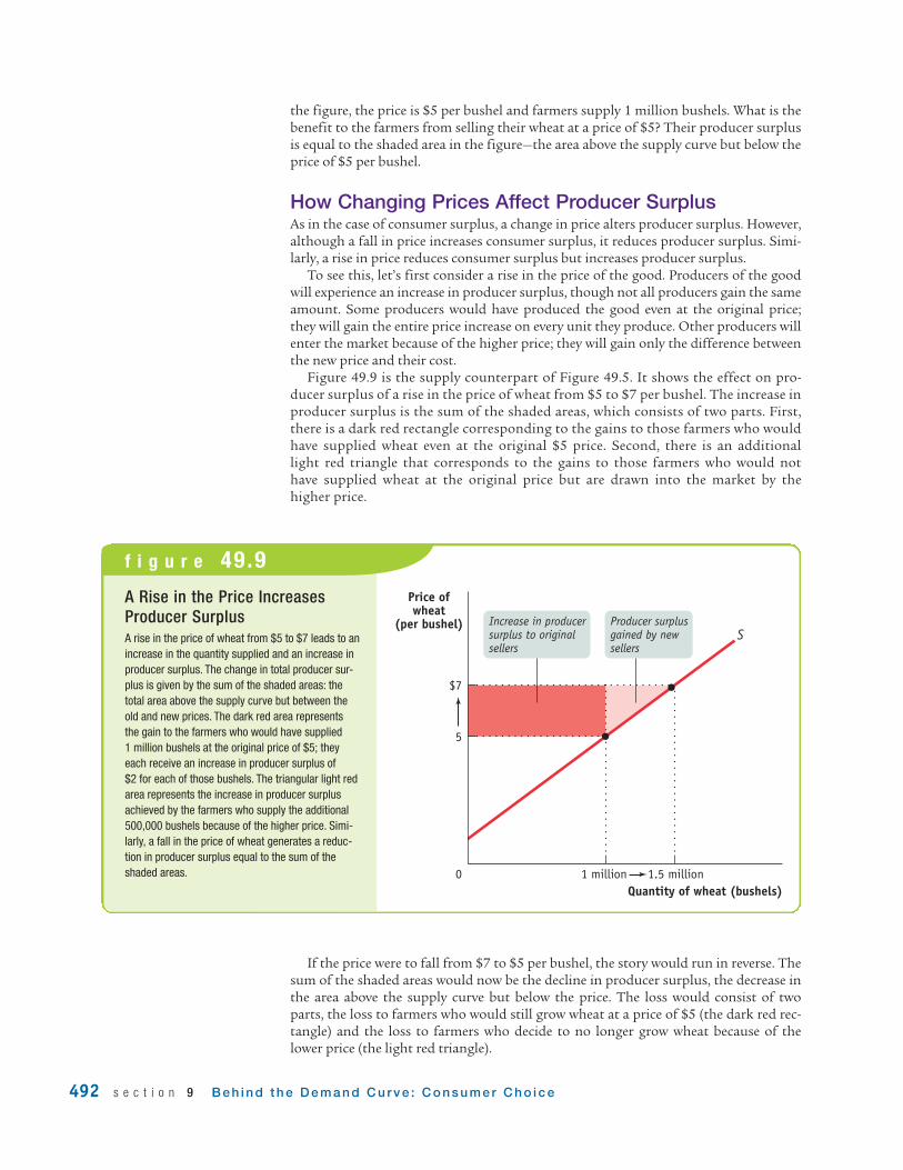
Figure 49.9 is the supply counterpart of Figure 49.5. It shows the effect on pro-ducer surplus of a rise in the price of wheat from $5 to $7 per bushel. The increase inproducer surplus is the sum of the shaded areas, which consists of two parts. First,there is a dark red rectangle corresponding to the gains to those farmers who wouldhave supplied wheat even at the original $5 price. Second, there is an additionallight red triangle that corresponds to the gains to those farmers who would nothave supplied wheat at the original price but are drawn into the market by thehigher price.

492 s e c t i o n 9 B e h i n d t h e D e m a n d C u r v e : C o n s u m e r C h o i c e

f i g u r e 49.9A Rise in the Price IncreasesProducer SurplusA rise in the price of wheat from $5 to $7 leads to anincrease in the quantity supplied and an increase inproducer surplus. The change in total producer sur-plus is given by the sum of the shaded areas: thetotal area above the supply curve but between theold and new prices. The dark red area representsthe gain to the farmers who would have supplied 1 million bushels at the original price of $5; theyeach receive an increase in producer surplus of $2 for each of those bushels. The triangular light redarea represents the increase in producer surplusachieved by the farmers who supply the additional500,000 bushels because of the higher price. Simi-larly, a fall in the price of wheat generates a reduc-tion in producer surplus equal to the sum of theshaded areas. 1.5 million

$7

5

Price ofwheat

(per bushel)

Quantity of wheat (bushels)1 million0

SIncrease in producer surplus to original sellers

Producer surplus gained by new sellers

If the price were to fall from $7 to $5 per bushel, the story would run in reverse. Thesum of the shaded areas would now be the decline in producer surplus, the decrease inthe area above the supply curve but below the price. The loss would consist of twoparts, the loss to farmers who would still grow wheat at a price of $5 (the dark red rec-tangle) and the loss to farmers who decide to no longer grow wheat because of thelower price (the light red triangle).

m o d u l e 4 9 C o n s u m e r a n d P ro d u c e r S u r p l u s 493

Section 9 Behind the Demand Curve: Consum

er Choice

M o d u l e 49 AP R e v i e w

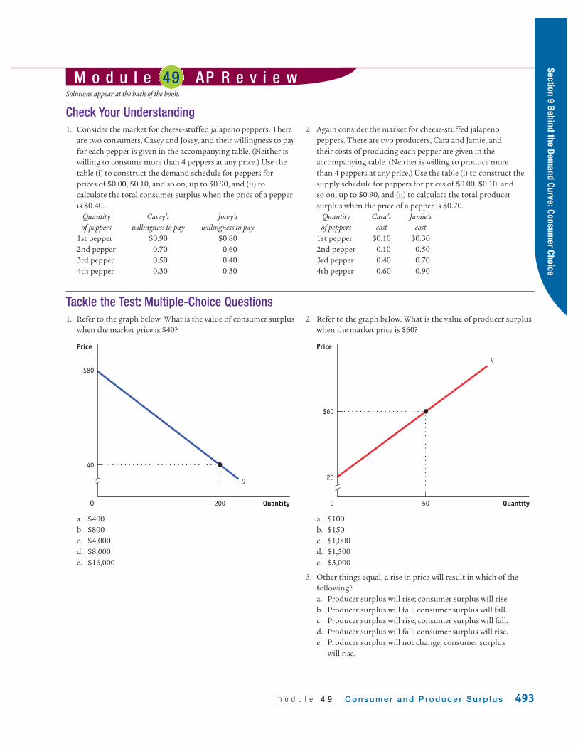
Check Your Understanding 1. Consider the market for cheese-stuffed jalapeno peppers. There

are two consumers, Casey and Josey, and their willingness to payfor each pepper is given in the accompanying table. (Neither iswilling to consume more than 4 peppers at any price.) Use thetable (i) to construct the demand schedule for peppers forprices of $0.00, $0.10, and so on, up to $0.90, and (ii) tocalculate the total consumer surplus when the price of a pepperis $0.40.

Quantity Casey’s Josey’sof peppers willingness to pay willingness to pay

1st pepper $0.90 $0.802nd pepper 0.70 0.603rd pepper 0.50 0.404th pepper 0.30 0.30

2. Again consider the market for cheese-stuffed jalapeno peppers. There are two producers, Cara and Jamie, and their costs of producing each pepper are given in theaccompanying table. (Neither is willing to produce more than 4 peppers at any price.) Use the table (i) to construct thesupply schedule for peppers for prices of $0.00, $0.10, and so on, up to $0.90, and (ii) to calculate the total producersurplus when the price of a pepper is $0.70.

Quantity Cara’s Jamie’sof peppers cost cost

1st pepper $0.10 $0.302nd pepper 0.10 0.503rd pepper 0.40 0.704th pepper 0.60 0.90

Solutions appear at the back of the book.

Tackle the Test: Multiple-Choice Questions1. Refer to the graph below. What is the value of consumer surplus

when the market price is $40?

a. $400b. $800c. $4,000d. $8,000e. $16,000

2000

Price

Quantity

D

40

$80

2. Refer to the graph below. What is the value of producer surpluswhen the market price is $60?

a. $100b. $150c. $1,000d. $1,500e. $3,000

3. Other things equal, a rise in price will result in which of thefollowing?a. Producer surplus will rise; consumer surplus will rise.b. Producer surplus will fall; consumer surplus will fall.c. Producer surplus will rise; consumer surplus will fall.d. Producer surplus will fall; consumer surplus will rise.e. Producer surplus will not change; consumer surplus

will rise.

Price

Quantity

$60

20

500

S

494 s e c t i o n 9 B e h i n d t h e D e m a n d C u r v e : C o n s u m e r C h o i c e

4. Consumer surplus is found as the areaa. above the supply curve and below the price.b. below the demand curve and above the price.c. above the demand curve and below the price.d. below the supply curve and above the price.e. below the supply curve and above the demand curve.

5. Allocating kidneys to those with the highest net benefit (wherenet benefit is measured as the expected increase in lifespanfrom a transplant) is an attempt to maximizea. consumer surplus.b. producer surplus.c. profit.d. equity.e. respect for elders.

Tackle the Test: Free-Response Questions1. Refer to the graph provided.

a. Calculate consumer surplus.b. Calculate producer surplus.c. If supply increases, what will happen to consumer surplus?

Explain.d. If demand decreases, what will happen to producer surplus?

Explain.

Price

Quantity200

40

$80

10

0

D

S

Answer (6 points)

1 point: $4,000

1 point: $3,000

1 point: Consumer surplus will increase.

1 point: An increase in supply lowers the equilibrium price, which causesconsumer surplus to increase.

1 point: Producer surplus will decrease.

1 point: A decrease in demand decreases the equilibrium price, which causesproducer surplus to decrease.

2. Draw a correctly labeled graph showing a competitive market inequilibrium. On your graph, clearly indicate and label the areaof consumer surplus and the area of producer surplus.