

Module 2: Planning and operation of distribution network
51
Module 2: Planning and operation of distribution network Lecture 1: Introduction to distribution networks Modelling and tools for the planning and operation of distribution network Alireza Bahmanyar, Prof. Damien Ernst
Transcript of Module 2: Planning and operation of distribution network
Module 2:
Planning and operation of distribution networkLecture 1: Introduction to distribution networksModelling and tools for the planning and operation of distribution network
Alireza Bahmanyar, Prof. Damien Ernst
Content
2
1
3
2
4
Distribution network equipment
Distribution network loads
Components modelling
Distribution network analysis

Distribution network structureA general view of substations, networks and components
3
1
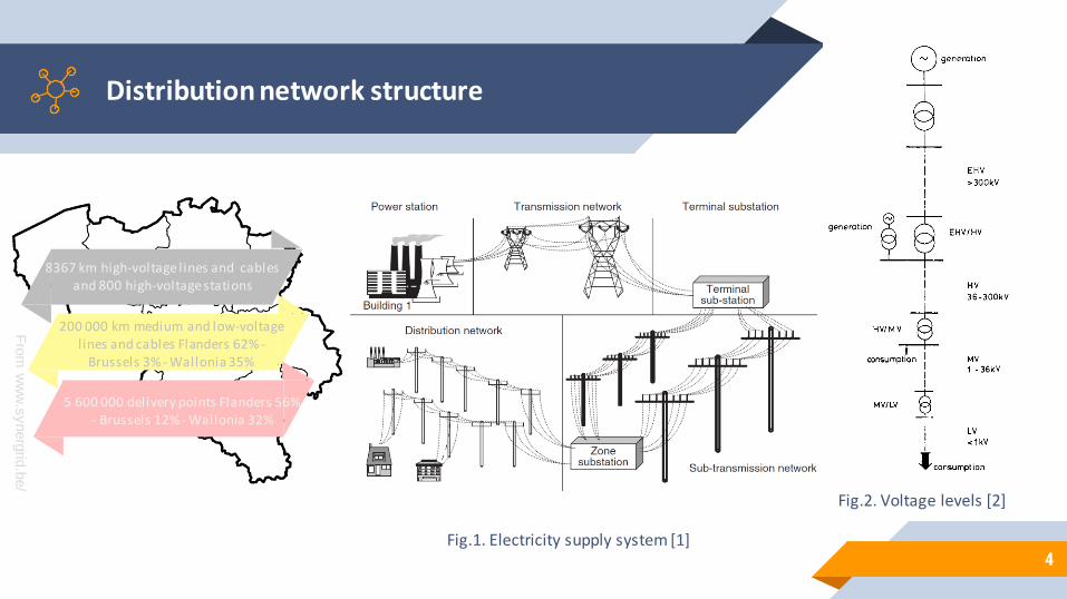
Distribution network structure
4Fig.1. Electricity supply system [1]
Fig.2. Voltage levels [2]
8367 km high-voltage lines and cables and 800 high-voltagestations
200 000 km medium and low-voltage lines and cables Flanders 62% -
Brussels 3% - Wallonia 35%
5 600 000 delivery points Flanders 56% - Brussels 12% - Wallonia 32%
Fro
m w
ww
.synerg
rid.b
e/
5
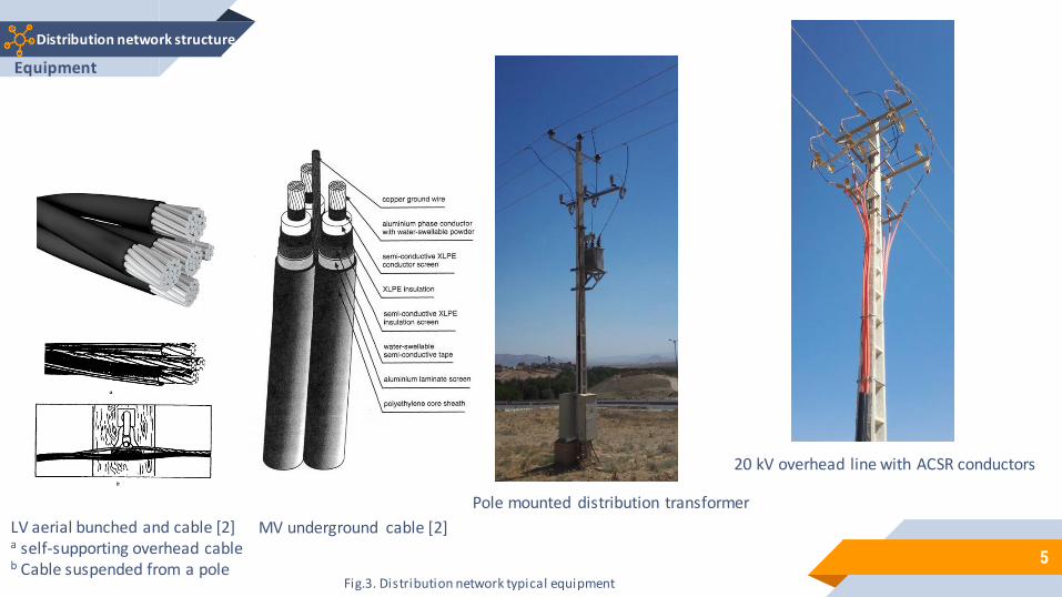
Distribution network structure
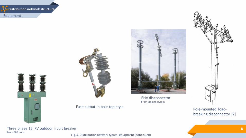
Fig.3. Distribution network typical equipment
20 kV overhead line with ACSR conductors
MV underground cable [2]LV aerial bunched and cable [2]a self-supporting overhead cableb Cable suspended from a pole
Pole mounted distribution transformer
Equipment
6
Distribution network structure
Three phase 15 KV outdoor ircuit breakerFrom ABB.com
Fuse cutout in pole-top stylePole-mounted load-breaking disconnector [2]
Fig.3. Distribution network typical equipment (continued)
EHV disconnectorFrom Siemence.com
Equipment
7
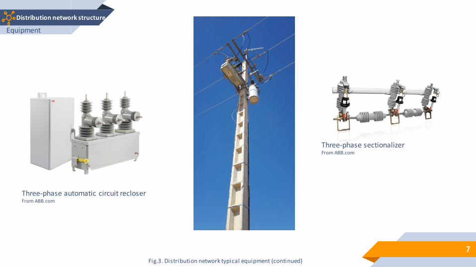
Distribution network structure
Three-phase automatic circuit recloserFrom ABB.com
Fig.3. Distribution network typical equipment (continued)
Three-phase sectionalizerFrom ABB.com
Equipment
8
Distribution network structure
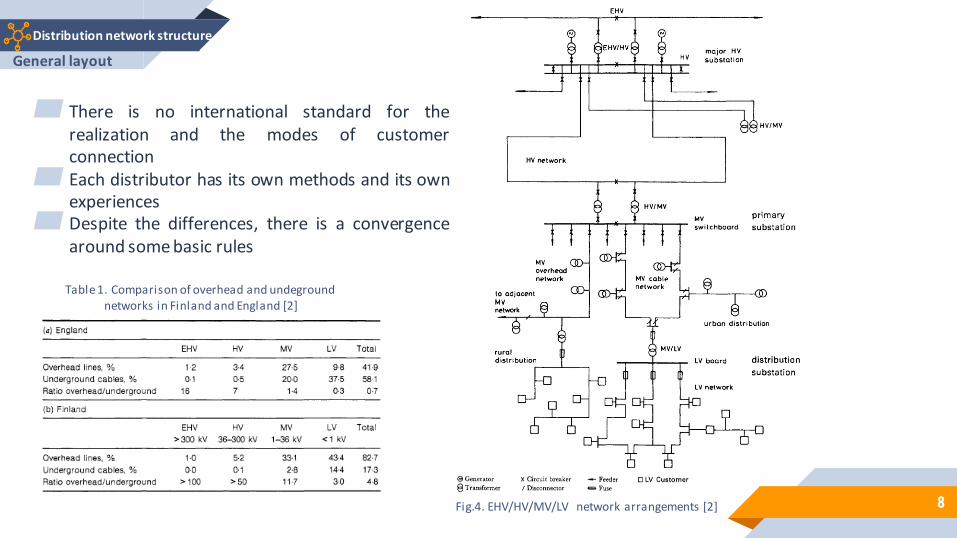
Fig.4. EHV/HV/MV/LV network arrangements [2]
▰ There is no international standard for therealization and the modes of customerconnection
▰ Each distributor has its own methods and its ownexperiences
▰ Despite the differences, there is a convergencearound some basic rules
Table 1. Comparison of overhead and undeground networks in Finland and England [2]
General layout
9
Distribution network structure
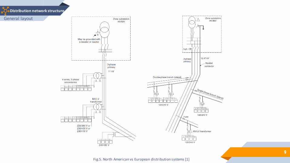
Fig.5. North American vs European distribution systems [1]
General layout
10
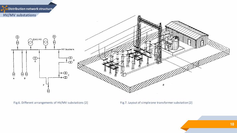
Distribution network structure
Fig.6. Different arrangements of HV/MV substations [2] Fig.7. Layout of simple one transformer substation [2]
HV/MV substations
11
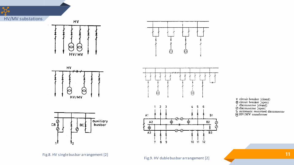
Distribution network structure
Fig.8. HV single busbar arrangement [2]Fig.9. HV duble busbar arrangement [2]
HV/MV substations

12
Distribution network structure
Fig.10. Schematic of typical MV overhead radial feeder [2] Fig.11. MV underground loop arrangements [2]
MV network
13
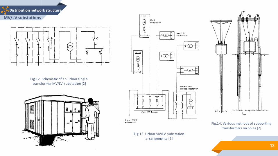
Distribution network structure
Fig.12. Schematic of an urban single-transformer MV/LV substation [2]
Fig.13. Urban MV/LV substation arrangements [2]
MV/LV substations
Fig.14. Various methods of supporting transformers on poles [2]

14
Distribution network structure
Fig.15. Typical L V systemsa. Rural, b. Urban [2]
LV network
15
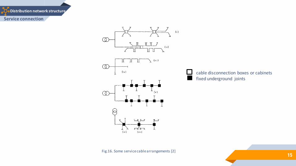
Distribution network structure
Fig.16. Some service cable arrangements [2]
Service connection
cable disconnection boxes or cabinetsfixed underground joints
Distribution network loadsLoad profiles, descriptive factors, and special loads
16
2
Distribution network loads
17
▰ The present and estimated future demand levels influence the sizes ofindividual lines and cables and other equipment, and also the optimumsystem configuration as a whole, e.g. substation density.
▰ It determines among several other factors the network design and timing ofmajor reinforcements.
▰ Undervoltages and losess at peak demands and undervoltages
18
Distribution network loads
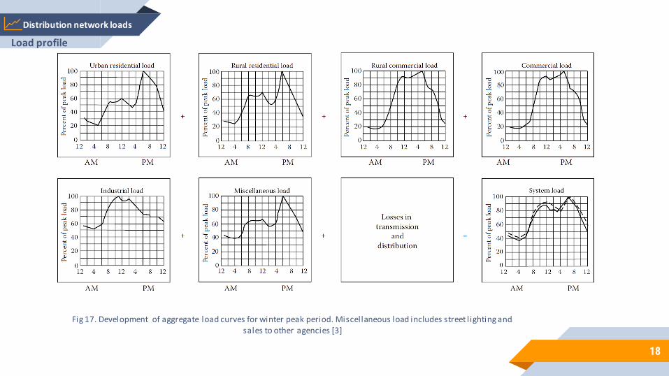
Fig 17. Development of aggregate load curves for winter peak period. Miscellaneous load includes street l ighting and sales to other agencies [3]
Load profile

19
Distribution network loads
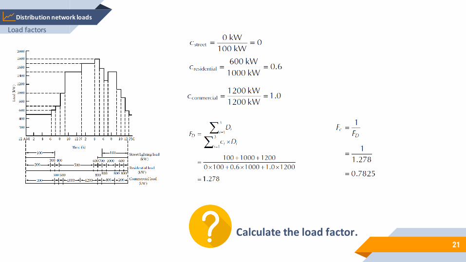
Fig.18. Daily load curve of a primary feeder for a typical winter day [3]
Table 2. Daily load data of a primary feeder for a typical winter day [3]
Load profile
20
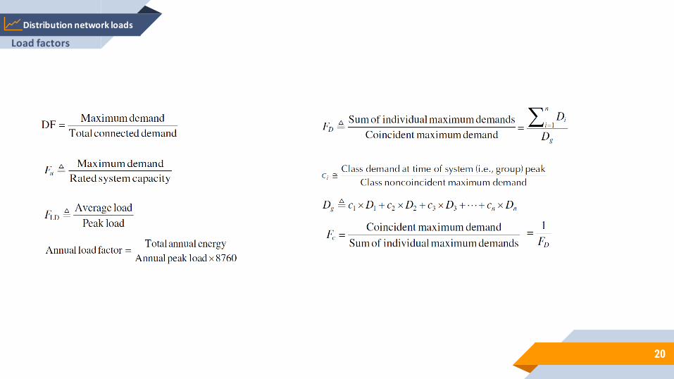
Distribution network loads
Load factors
21
Distribution network loads
Calculate the load factor.
Load factors
22
Distribution network loads
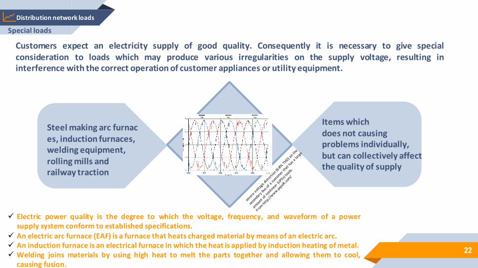
Customers expect an electricity supply of good quality. Consequently it is necessary to give specialconsideration to loads which may produce various irregularities on the supply voltage, resulting ininterference with the correct operation of customer appliances or utility equipment.
✓ Electric power quality is the degree to which the voltage, frequency, and waveform of a powersupply system conform to established specifications.
✓ An electric arc furnace (EAF) is a furnace that heats charged material by means of an electric arc.✓ An induction furnace is an electrical furnace in which the heat is applied by induction heating of metal.✓ Welding joins materials by using high heat to melt the parts together and allowing them to cool,
causing fusion.
Steel making arc furnaces, induction furnaces,welding equipment, rolling mills and railway traction
Items which does not causing problems individually, but can collectively affect the quality of supply
Special loads
23
Distribution network loads
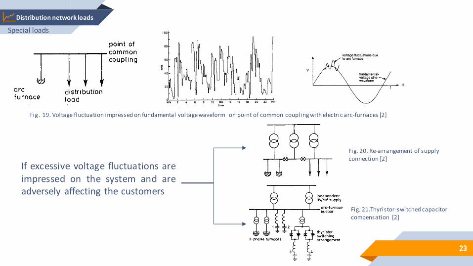
Fig . 19. Voltage fluctuation impressed on fundamental voltage waveform on point of common coupling with electric arc-furnaces [2]
If excessive voltage fluctuations areimpressed on the system and areadversely affecting the customers
Fig. 20. Re-arrangement of supply connection [2]
Fig. 21.Thyristor-switched capacitor compensation [2]
Special loads
24
Distribution network loads
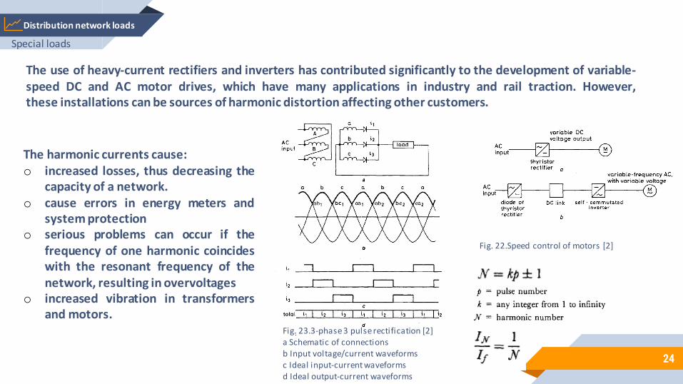
Fig. 22.Speed control of motors [2]
The use of heavy-current rectifiers and inverters has contributed significantly to the development of variable-speed DC and AC motor drives, which have many applications in industry and rail traction. However,these installations can be sources of harmonic distortion affecting other customers.
Fig. 23.3-phase 3 pulse rectification [2]a Schematic of connectionsb Input voltage/current waveformsc Ideal input-current waveformsd Ideal output-current waveforms
The harmonic currents cause:o increased losses, thus decreasing the
capacity of a network.o cause errors in energy meters and
system protectiono serious problems can occur if the
frequency of one harmonic coincideswith the resonant frequency of thenetwork, resulting in overvoltages
o increased vibration in transformersand motors.
Special loads

Components modellingModels for most common network elements
suitable for power flow analysis25
3
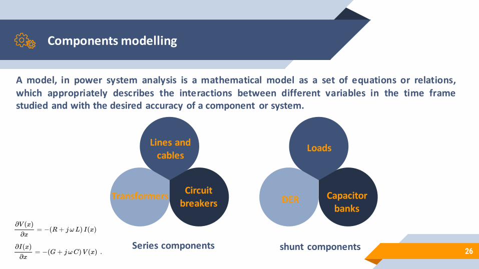
Components modelling
26Series components shunt components
Lines and cables
Transformers
Loads
DER Capacitor banks
Circuit breakers
A model, in power system analysis is a mathematical model as a set of equations or relations,which appropriately describes the interactions between different variables in the time framestudied and with the desired accuracy of a component or system.
27
Components modelling
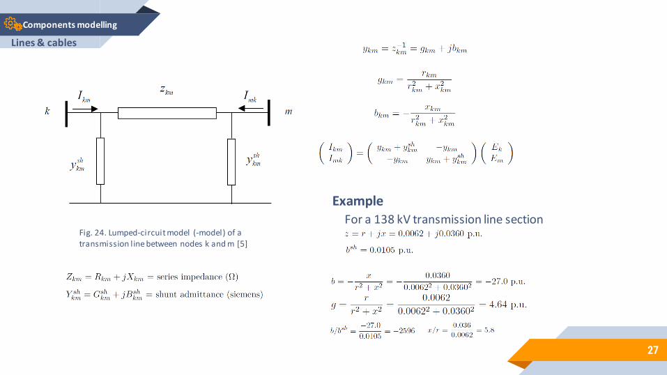
Fig. 24. Lumped-circuit model (-model) of a transmission line between nodes k and m [5]
For a 138 kV transmission line section
Example
Lines & cables
28
Components modelling
Lines & cables
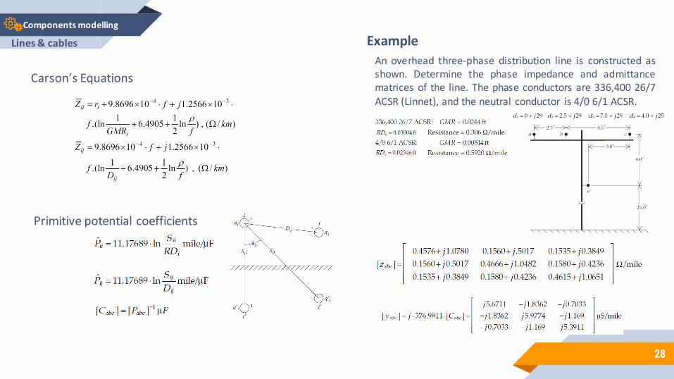
Carson’s Equations
Primitive potential coefficients
An overhead three-phase distribution line is constructed asshown. Determine the phase impedance and admittancematrices of the line. The phase conductors are 336,400 26/7ACSR (Linnet), and the neutral conductor is 4/0 6/1 ACSR.
Example
29
Components modelling
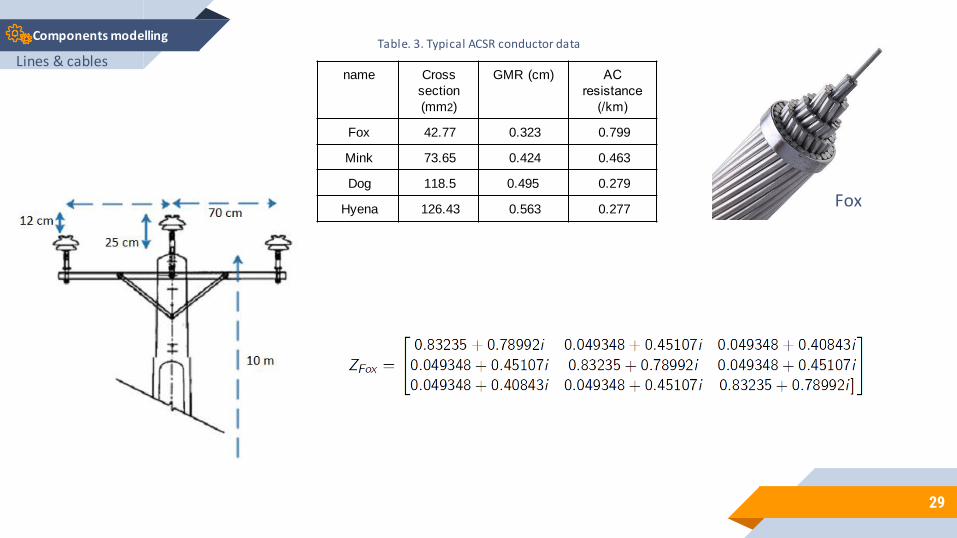
name Cross
section
(mm2)
GMR (cm) AC
resistance
(/km)
Fox 42.77 0.323 0.799
Mink 73.65 0.424 0.463
Dog 118.5 0.495 0.279
Hyena 126.43 0.563 0.277
Table. 3. Typical ACSR conductor data
Fox
Lines & cables
30
Components modelling
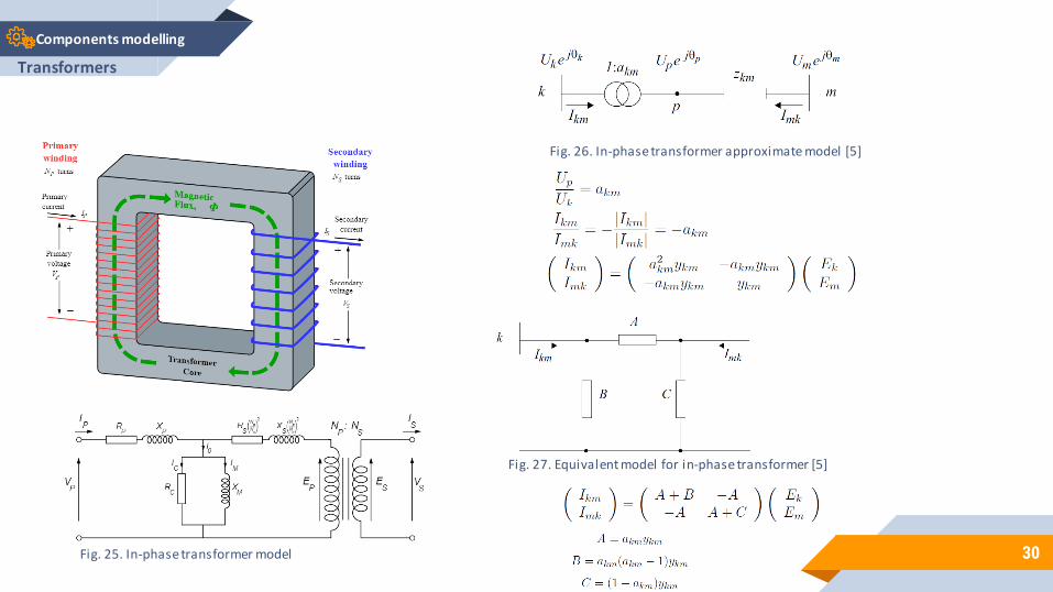
Fig. 25. In-phase transformer model
Fig. 26. In-phase transformer approximate model [5]
Fig. 27. Equivalent model for in-phase transformer [5]
Transformers
31
Components modelling
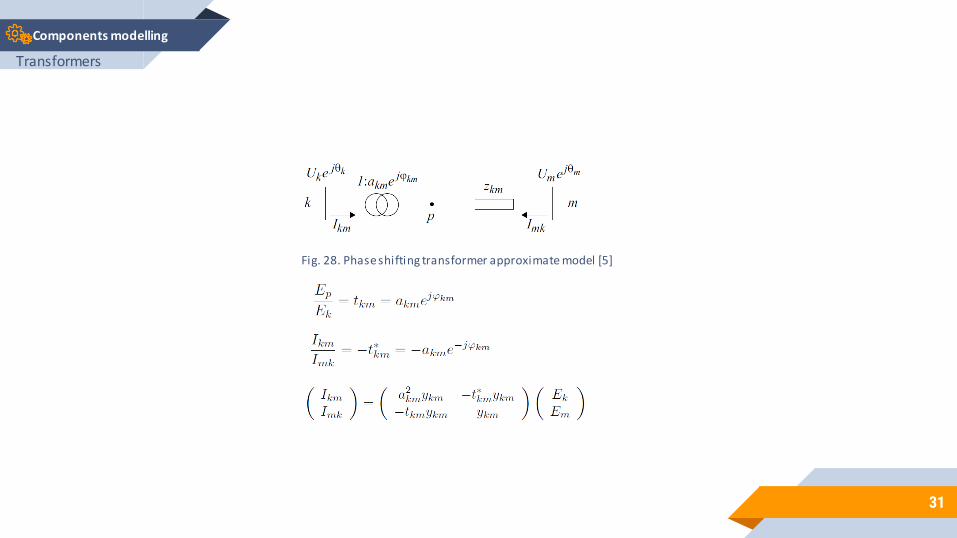
Fig. 28. Phase shifting transformer approximate model [5]
Transformers
32
Components modelling
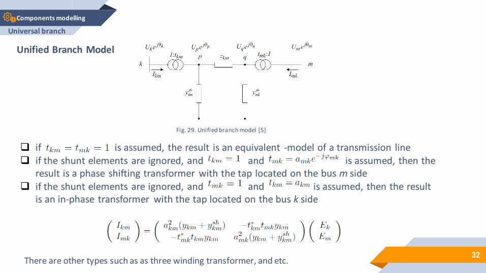
Unified Branch Model
Fig. 29. Unified branch model [5]
❑ if is assumed, the result is an equivalent -model of a transmission line❑ if the shunt elements are ignored, and and is assumed, then the
result is a phase shifting transformer with the tap located on the bus m side❑ if the shunt elements are ignored, and and is assumed, then the result
is an in-phase transformer with the tap located on the bus k side
There are other types such as as three winding transformer, and etc.
Universal branch
33
Components modelling
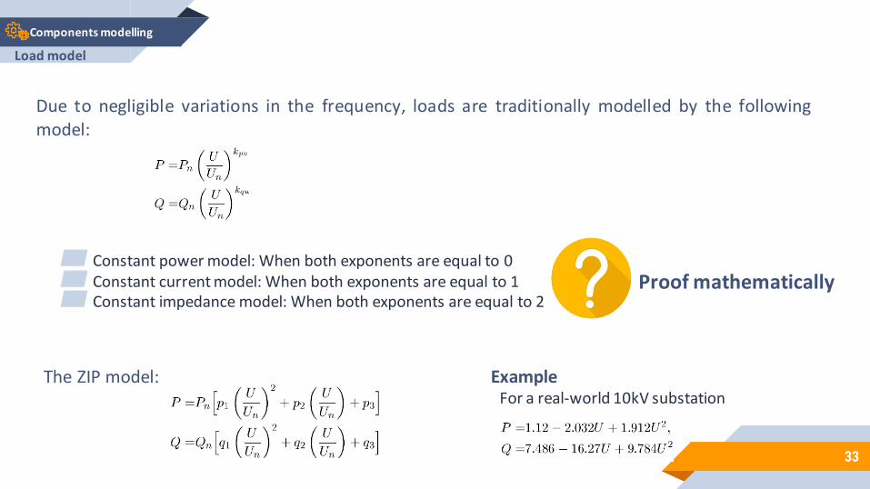
Due to negligible variations in the frequency, loads are traditionally modelled by the followingmodel:
▰ Constant power model: When both exponents are equal to 0▰ Constant current model: When both exponents are equal to 1▰ Constant impedance model: When both exponents are equal to 2
Proof mathematically
For a real-world 10kV substationThe ZIP model:
Load model
Example

Distribution network analysisLoad flow and state estimation formulation
34
4

Distribution network analysis
35
The inputs▰ Main substation voltage▰ Load data and their models▰ Network data including the topology, lines impedance, etc.
▰ Distribution systems are radial or weakly meshed network structures▰ They have high X/R ratios in the line impedances▰ They may have of many single-phase or two-phase loads and laterals
Distribution load flow
The outputs▰ Voltage magnitudes and angles at all nodes of the feeder▰ Line flow in each line section specified in kW and kvar, or amps
and degrees▰ Power loss in each line section and total feeder power losses▰ Total feeder input kW and kvar▰ Load kW and kvar based upon the specified model for the load
36
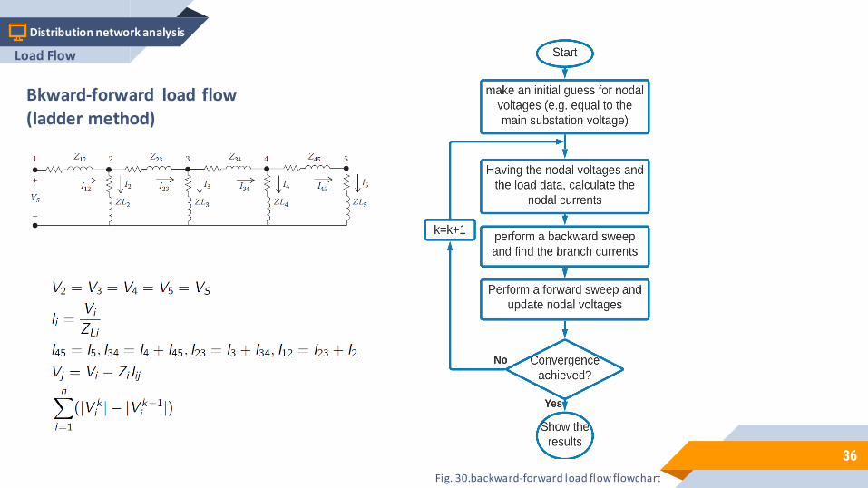
Distribution network analysis t
Bkward-forward load flow(ladder method)
Fig. 30.backward-forward load flow flowchart
Load Flow
37
Distribution network analysis t
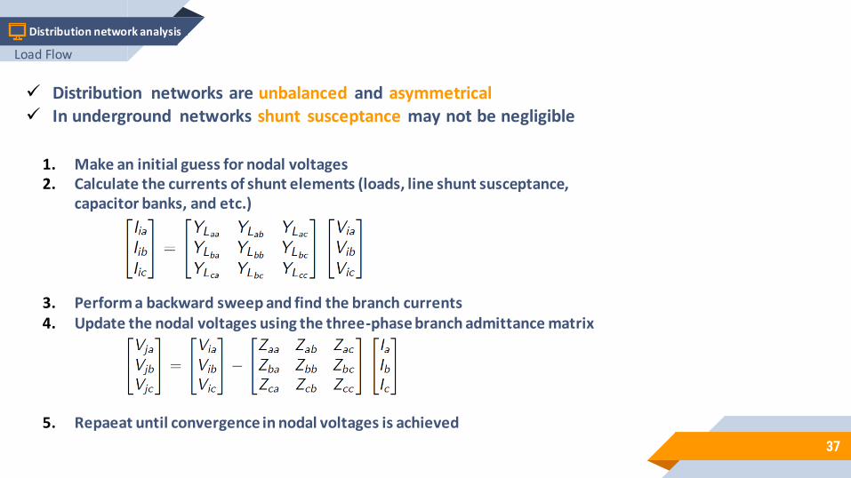
✓ Distribution networks are unbalanced and asymmetrical✓ In underground networks shunt susceptance may not be negligible
1. Make an initial guess for nodal voltages2. Calculate the currents of shunt elements (loads, line shunt susceptance,
capacitor banks, and etc.)
3. Perform a backward sweep and find the branch currents4. Update the nodal voltages using the three-phase branch admittance matrix
5. Repaeat until convergence in nodal voltages is achieved
Load Flow

38
Distribution network analysis t
Distribution state estimation
In any distribution network with a set of measurements (Z), the relation between networkstate variables (x) and the measurements can be described as follows:
where h represents the relation between the measurements and the state variables and e isthe measurement error.
For example in the following figure which presents a portion of a distribution network, assume thatthe line suceptance is negligible, the line impedances are known, and the lines currents and thevoltages of nodes 1 and 3 are measured. To obtan the voltage of node 2 we have:
Considering the errors in measurements, the obtained values will not be equal
State estimation
39
Distribution network analysis t
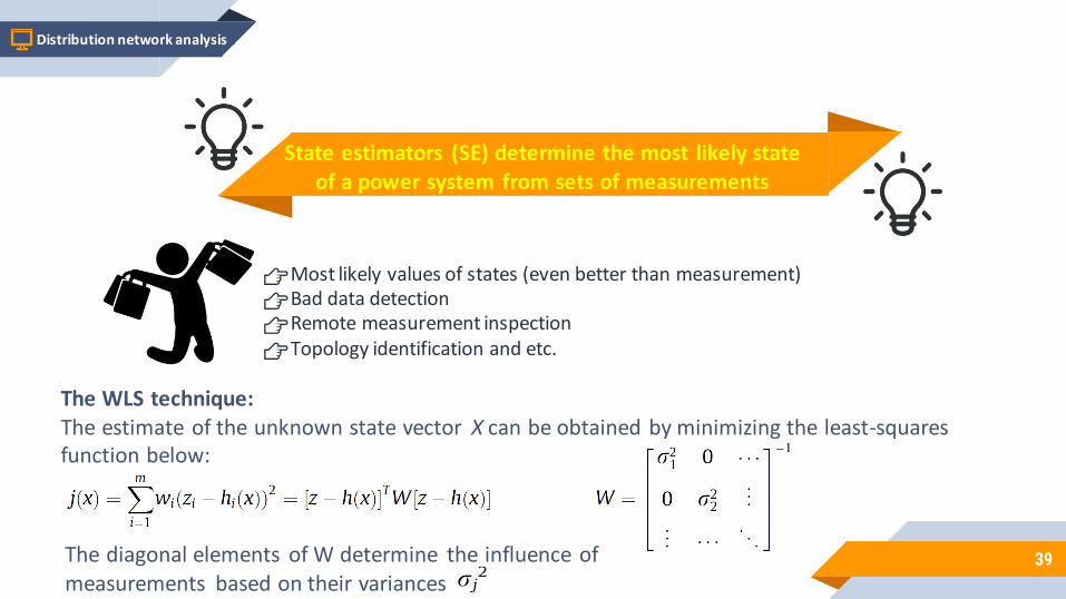
State estimators (SE) determine the most likely state of a power system from sets of measurements
👉Most likely values of states (even better than measurement)👉Bad data detection👉Remote measurement inspection👉Topology identification and etc.
The WLS technique:The estimate of the unknown state vector X can be obtained by minimizing the least-squares function below:
The diagonal elements of W determine the influence of measurements based on their variances
State estimation
40
Distribution network analysis t
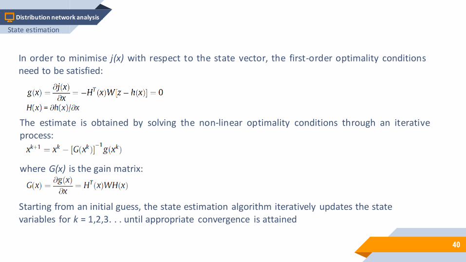
In order to minimise j(x) with respect to the state vector, the first-order optimality conditionsneed to be satisfied:
The estimate is obtained by solving the non-linear optimality conditions through an iterativeprocess:
where G(x) is the gain matrix:
Starting from an initial guess, the state estimation algorithm iteratively updates the state variables for k = 1,2,3. . . until appropriate convergence is attained
State estimation
41
Distribution network analysis t
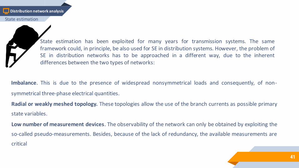
Imbalance. This is due to the presence of widespread nonsymmetrical loads and consequently, of non-
symmetrical three-phase electrical quantities.
Radial or weakly meshed topology. These topologies allow the use of the branch currents as possible primary
state variables.
Low number of measurement devices. The observability of the network can only be obtained by exploiting the
so-called pseudo-measurements. Besides, because of the lack of redundancy, the available measurements are
critical
State estimation has been exploited for many years for transmission systems. The sameframework could, in principle, be also used for SE in distribution systems. However, the problem ofSE in distribution networks has to be approached in a different way, due to the inherentdifferences between the two types of networks:
State estimation

42
Distribution network analysis t
High number of nodes. This (along with the need of developing three-phase estimators) leads to very large
systems, resulting in the explosion of execution times of the algorithms.
Network model uncertainty. In the SE framework, line impedances of the network are generally assumed to be
known. Actually, the knowledge of network model parameters has large uncertainty due to network aging and
lack of accurate measurement campaigns. This can lead to a degradation of SE performance.
Low X/R ratio. This leads to the impossibility of adopting simplifications commonly used in the estimators
developed for transmission systems, as for example, neglecting resistances because of dominant inductive
terms. As a further consequence, decoupled versions of the estimators are not so easily obtained.
State estimation
43
Distribution network analysis t
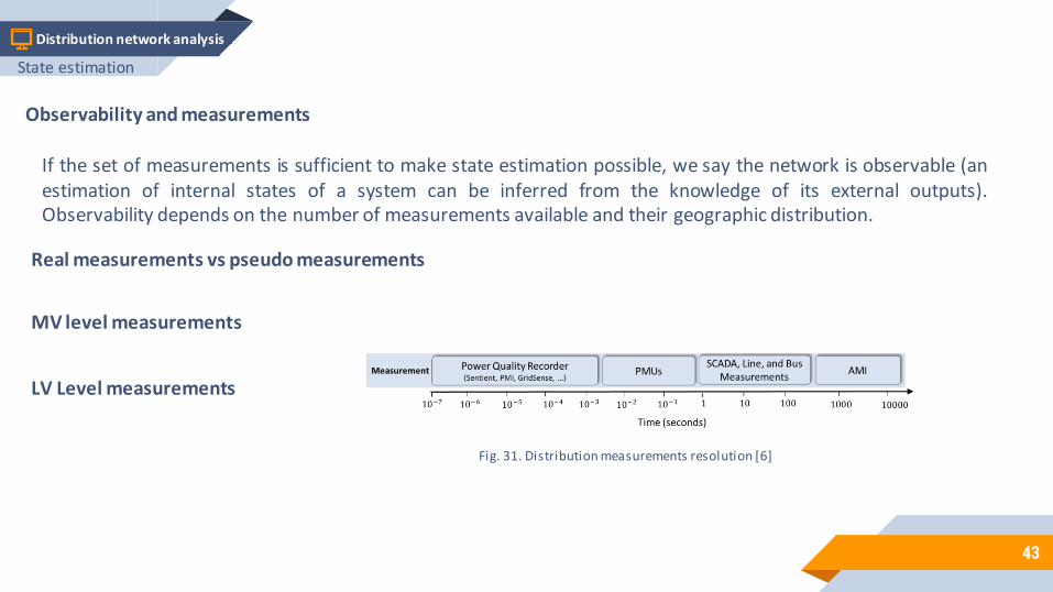
Observability and measurements
If the set of measurements is sufficient to make state estimation possible, we say the network is observable (anestimation of internal states of a system can be inferred from the knowledge of its external outputs).Observability depends on the number of measurements available and their geographic distribution.
Real measurements vs pseudo measurements
MV level measurements
LV Level measurements
Fig. 31. Distribution measurements resolution [6]
State estimation
44
Distribution network analysis t
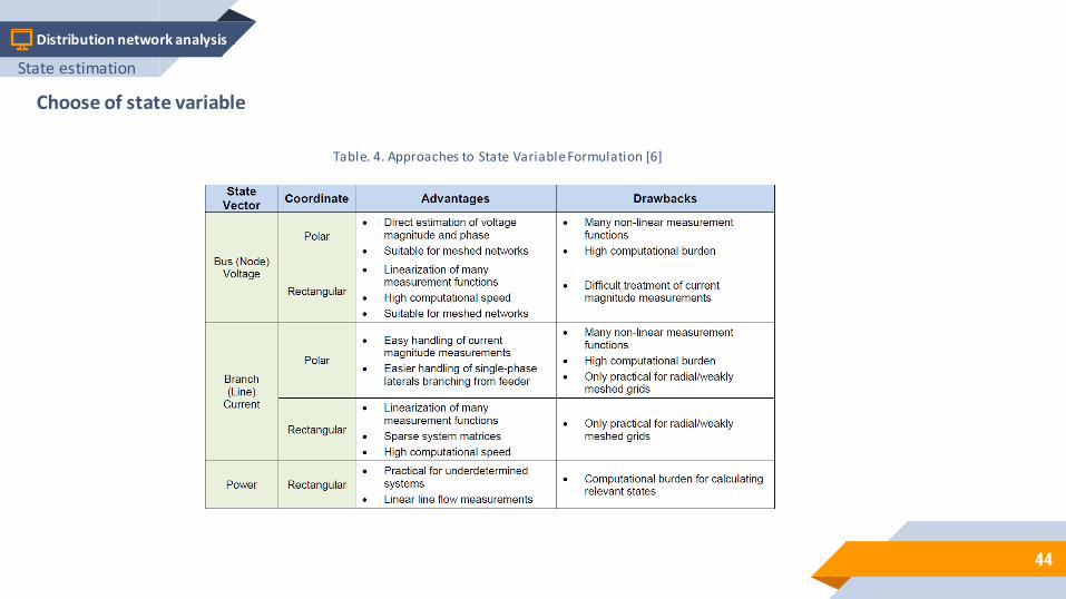
Choose of state variable
Table. 4. Approaches to State Variable Formulation [6]
State estimation
45
Distribution network analysis t
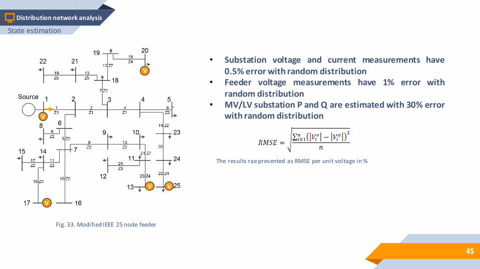
Fig. 33. Modified IEEE 25 node feeder
VV
V
V
V
• Substation voltage and current measurements have0.5% error with random distribution
• Feeder voltage measurements have 1% error withrandom distribution
• MV/LV substation P and Q are estimated with 30% errorwith random distribution
The results rae presented as RMSE per unit voltage in %
State estimation

46
Distribution network analysis t
Scenario 1: Accurate load estimates and measurements
State estimation
47
Distribution network analysis t
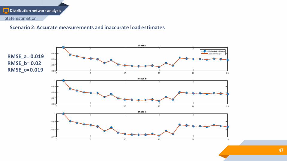
Scenario 2: Accurate measurements and inaccurate load estimates
RMSE_a= 0.019RMSE_b= 0.02RMSE_c= 0.019
State estimation

48
Distribution network analysis t
Scenario 3: Accurate measurements and inaccurate load estimatesVoltage measurements at nodes 20 and 17 are not available
RMSE_a= 0.034RMSE_b= 0.035RMSE_c= 0.029
State estimation

49
Distribution network analysis t
Scenario 4: Inaccurate measurements and inaccurate load estimates
RMSE_a= 0.53RMSE_b= 0.36RMSE_c= 0.67
State estimation

References
1. Sallam, A.A. and Malik, O.P., 2018. Electric distribution systems, Wiley.2. Lakervi, E. and Holmes, E.J., 1995. Electricity distribution network design, IET.3. Gonen, T., 2015. Electric power distribution engineering. CRC press.4. Kersting, William H. 2017. Distribution system modeling and analysis. CRC press.5. G. Andersson. 2004, Modelling and analysis of electric power systems. EEH-Power SystemsLaboratory, Swiss Federal Institute of Technology (ETH), Zurich, Switzerland.6. NYSE Research and DA (NYSERDA), 2018. Fundamental research challenges for distribution state estimation to enable high-performing grids, NYSERDA Report Prepared by Smarter Grid Solutions.
50