Modular Lattices for Compositional Interprocedural Analysis · I would like to thank Dr. Mayur Naik...
80
Tel Aviv University Raymond and Beverly Sackler Faculty of Exact Sciences School of Computer Science Modular Lattices for Compositional Interprocedural Analysis by Ghila Castelnuovo under the supervision of Prof. Mooly Sagiv Thesis submitted in partial fulfilment of the requirements for the degree of Master of Science September 2012 Elul 5772
Transcript of Modular Lattices for Compositional Interprocedural Analysis · I would like to thank Dr. Mayur Naik...

Tel Aviv UniversityRaymond and Beverly Sackler Faculty of Exact Sciences
School of Computer Science
Modular Lattices for Compositional Interprocedural
Analysis
by
Ghila Castelnuovo
under the supervision ofProf. Mooly Sagiv
Thesis submitted in partial fulfilment of the requirementsfor the degree of Master of Science
September 2012 Elul 5772
Abstract
Modular Lattices for Compositional Interprocedural Analysis
Ghila CastelnuovoMaster of Science
School of Computer ScienceTel-Aviv University
Interprocedural analyses are compositional when they compute over-approximations of proce-
dures in a bottom-up fashion. These analyses are usually more scalable than top-down analyses,
which compute a different procedure summary for every calling context. However, composi-
tional analyses are rare in practice as it is difficult to develop them with enough precision.
In this work, we establish a connection between compositional analyses and so called modu-
lar lattices, which require certain associativity between the lattice join and meet operations.
Our connection provides sufficient conditions for building a compositional analysis that has the
same precision as a top-down analysis. It also sheds light on the limitations of our approach:
the transfer functions must have to be expressed as joins and meets with constant elements.
Following our recipe, we develop a compositional version of the connection analysis by Ghiya
and Hendren, which was motivated by the need to parallelize sequential code. Our version is
slightly more conservative than the original top-down analysis in order to meet our modularity
requirement. We applied our compositional connection analysis to real-world Java programs
and, as expected, the analysis scaled much better than the original top-down version. The
top-down analysis times out in the largest two of our five programs, and only 2-5% of precision
is lost due to the modularity requirement in the remaining programs.
ii
Acknowledgements
I would like to express my gratitude to all of those who contributed to the completion of mythesis.
First and foremost, I would like to thank Prof. Mooly Sagiv, for his guidance, knowledge,passion, optimism and above all - encouragement and support. I have been very fortunate tohave him as my advisor.
Also, I would not have completed this work without the help of Dr. Noam Rinetzky. Iwould like to thank him for his guidance, endless patience and dedication.
I would like to thank Dr. Mayur Naik and Dr. Hongseok Yang for their time, insightfulcomments and for inspiring me. It has been a privilege working with them.
A warm thanks goes to my colleagues and friends Guy Gueta, Shachar Itzhaky, OhadShacham, Omer Tripp and Or Tamir for their advices and encouragement.
Finally, I would like to thank my great family and my beloved husband, for their love, moralsupport and constant encouragement.
iii

Contents
1 Introduction 1
2 Informal Explanation 3
2.1 A Motivating Example . . . . . . . . . . . . . . . . . . . . . . . . . . . . . . . . . 3
2.2 Connection Analysis and Points-to Analysis . . . . . . . . . . . . . . . . . . . . . 3
2.3 Top-Down Interprocedural Analysis . . . . . . . . . . . . . . . . . . . . . . . . . 6
2.4 Bottom-Up Compositional Interprocedural Analysis . . . . . . . . . . . . . . . . 6
2.5 Modular Lattices for Bottom-Up Compositional Interprocedural Analysis . . . . 6
3 Preliminaries 8
3.1 Programming Language . . . . . . . . . . . . . . . . . . . . . . . . . . . . . . . . 8
3.1.1 Standard Semantics . . . . . . . . . . . . . . . . . . . . . . . . . . . . . . 9
3.1.2 Relational Collecting Semantics . . . . . . . . . . . . . . . . . . . . . . . . 9
3.2 Modularity in Lattices . . . . . . . . . . . . . . . . . . . . . . . . . . . . . . . . . 10
4 Intraprocedural Analysis using Modularity 11
4.1 Intraprocedural Connection Analysis . . . . . . . . . . . . . . . . . . . . . . . . . 11
4.1.1 Partition Domains . . . . . . . . . . . . . . . . . . . . . . . . . . . . . . . 11
4.2 Conditionally Compositional Intraprocedural Analysis . . . . . . . . . . . . . . . 13
5 Compositional Analysis using Modularity 15
5.1 Compositional Connection Analysis . . . . . . . . . . . . . . . . . . . . . . . . . . 15
5.1.1 Partition Domains for Ternary Relations . . . . . . . . . . . . . . . . . . . 15
5.1.2 Triad Partition Domains . . . . . . . . . . . . . . . . . . . . . . . . . . . . 16
5.1.3 Interprocedural Top Down Triad Connection Analysis . . . . . . . . . . . 18
5.1.4 Bottom Up Triad Connection Analysis . . . . . . . . . . . . . . . . . . . . 20
5.1.5 Coincidence Result in Connection Analysis . . . . . . . . . . . . . . . . . 20
5.2 Compositional Analysis . . . . . . . . . . . . . . . . . . . . . . . . . . . . . . . . 28
5.2.1 Triad Domains . . . . . . . . . . . . . . . . . . . . . . . . . . . . . . . . . 28
5.2.2 Interprocedural Triad Analysis . . . . . . . . . . . . . . . . . . . . . . . . 32
5.2.3 Coincidence Result . . . . . . . . . . . . . . . . . . . . . . . . . . . . . . . 33
5.3 Computing Abstract States Using Compositional Summaries . . . . . . . . . . . 38
6 Implementation and Experimental Evaluation 42
6.1 Implementation . . . . . . . . . . . . . . . . . . . . . . . . . . . . . . . . . . . . . 42
6.1.1 Top Down Analyses . . . . . . . . . . . . . . . . . . . . . . . . . . . . . . 42
6.1.2 Bottom Up Analysis . . . . . . . . . . . . . . . . . . . . . . . . . . . . . . 43
6.2 Experimental Evaluation . . . . . . . . . . . . . . . . . . . . . . . . . . . . . . . . 44
iv

6.2.1 Precision . . . . . . . . . . . . . . . . . . . . . . . . . . . . . . . . . . . . 466.2.2 Scalability . . . . . . . . . . . . . . . . . . . . . . . . . . . . . . . . . . . . 47
7 Conclusions 48
A Appendix 51A.1 Intraprocedural Adaptable Analysis . . . . . . . . . . . . . . . . . . . . . . . . . 51A.2 Triad Connection Analysis . . . . . . . . . . . . . . . . . . . . . . . . . . . . . . . 53
A.2.1 Galois Connection . . . . . . . . . . . . . . . . . . . . . . . . . . . . . . . 54A.2.2 Connection Analysis as a Triad Analysis . . . . . . . . . . . . . . . . . . . 56
A.3 Triad Copy Constant Propagation Analysis . . . . . . . . . . . . . . . . . . . . . 63A.3.1 Programming Language . . . . . . . . . . . . . . . . . . . . . . . . . . . . 63A.3.2 Concrete Semantics . . . . . . . . . . . . . . . . . . . . . . . . . . . . . . 64A.3.3 Abstract Semantics . . . . . . . . . . . . . . . . . . . . . . . . . . . . . . . 64A.3.4 Soundness of the Top Down Analysis . . . . . . . . . . . . . . . . . . . . . 68A.3.5 Precision Improving Transformations . . . . . . . . . . . . . . . . . . . . . 68A.3.6 Copy Constant Propagation as a Triad Analysis . . . . . . . . . . . . . . 68
v

List of Tables
4.1 Abstract transfer functions for primitive commands in the connection analysis.In Section 4.1.1.1, x is x and y is y. In Section 5.1, x denotes x′ and y denotes y′. 13
4.2 Auxiliary constants used in the abstract semantics shown in Table 4.1. Uxy isused to merge x and y’s connection sets. Sx is used to separate x from its currentconnection set. . . . . . . . . . . . . . . . . . . . . . . . . . . . . . . . . . . . . . 13
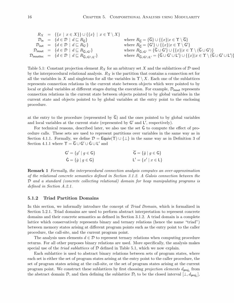
5.1 Constant projection element RX for an arbitrary set X and the sublattices of Dused by the interprocedural relational analysis. RX is the partition that containsa connection set for all the variables in X and singletons for all the variablesin Υ \ X. Each one of the sublattices represents connection relations in thecurrent state between objects which were pointed to by local or global variables atdifferent stages during the execution. For example, Dinout represents connectionrelations in the current state between objects pointed to by global variables inthe current state and objects pointed to by global variables at the entry point tothe enclosing procedure. . . . . . . . . . . . . . . . . . . . . . . . . . . . . . . . . 16
5.2 The definition of ιentry and the interprocedural abstract semantics for the top-down connection analysis. ιentry is the element that represents the identity rela-tion between input and output, and Cbodyp is the body of the procedure p. . . . . 18
5.3 Definition of ιentry and the interprocedural abstract semantics for the bottom-upconnection analysis. . . . . . . . . . . . . . . . . . . . . . . . . . . . . . . . . . . 20
5.4 Triad Analysis Abstract Semantics. The top-down triad analysis uses the seman-tic represented by the [[·]]] functions. The counterpart bottom-up triad analysisanalysis uses the same semantics, with the exception of the C = p() command,whose semantics is [[p()]]]BU. . . . . . . . . . . . . . . . . . . . . . . . . . . . . . 32
6.1 Benchmark characteristics. The “# of classes” column is the number of classescontaining reachable methods. The “# of methods” column is the number ofreachable methods computed by a static 0-CFA call-graph analysis. The “# ofbytecodes” column is the number of bytecodes of reachable methods. The “total”columns report numbers for all reachable code, whereas the “app only” columnsreport numbers for only application code (excluding JDK library code). . . . . . 44
6.2 The number of queries to connection analysis and three metrics comparing thescalability of the original top-down and our modular bottom-up versions of theanalysis on those queries: running time, memory consumption, and number ofincoming abstract states computed at program points of interest. These pointsinclude only query points in the “query” sub-columns and all points in the “total”sub-columns. All three metrics show that the top-down analysis scales much morepoorly than the bottom-up analysis. . . . . . . . . . . . . . . . . . . . . . . . . . 44
vi

6.3 The number of queries to connection analysis and three metrics representingthe scalability of the modular top-down version of the analysis on those queries:running time, memory consumption, and number of incoming abstract statescomputed at program points of interest. These points include only query pointsin the “query” sub-columns and all points in the “total” sub-columns. All threemetrics show that also the modular top-down analysis scales much more poorlythan the bottom-up analysis. . . . . . . . . . . . . . . . . . . . . . . . . . . . . . 46
A.1 Intraprocedural Abstract Semantics for Adaptable Analysis . . . . . . . . . . . . 51
vii

List of Figures
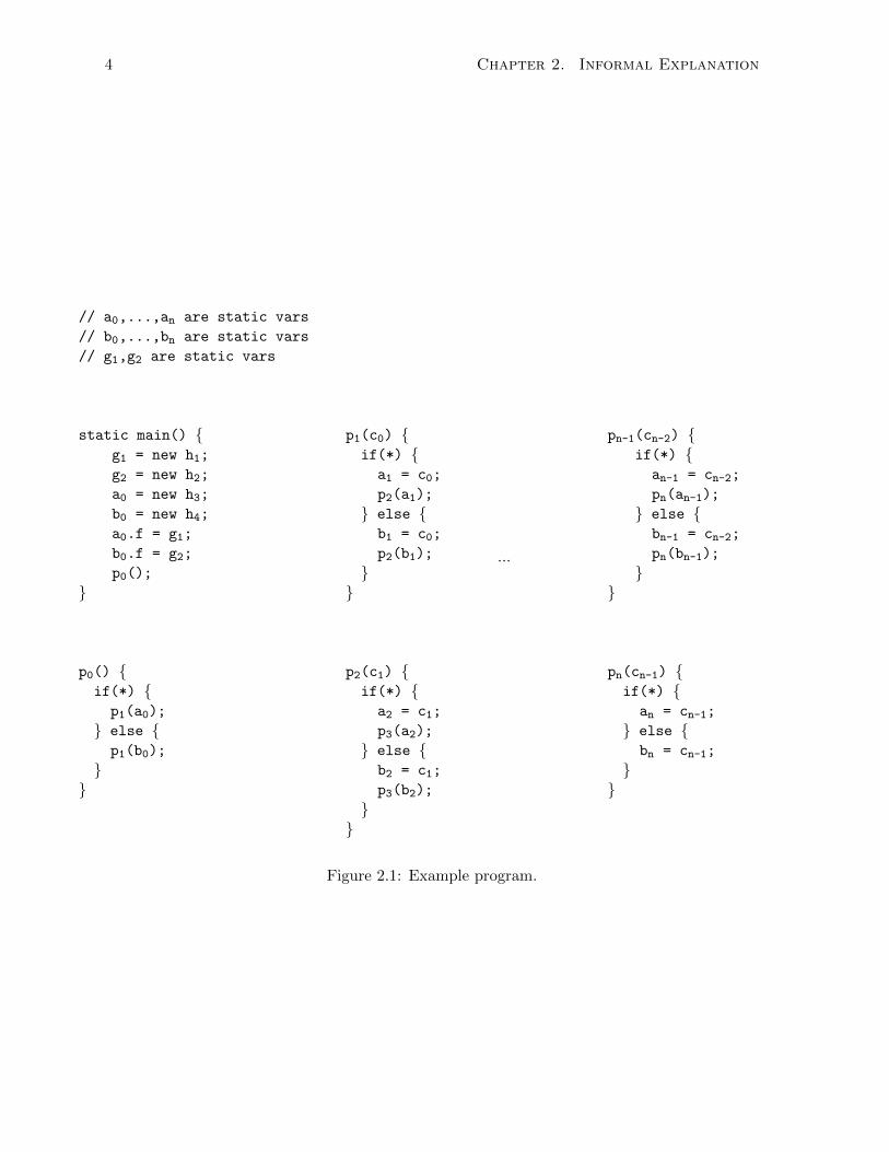
2.1 Example program. . . . . . . . . . . . . . . . . . . . . . . . . . . . . . . . . . . . 42.2 Concrete states at the entry of procedure p1 of the program in Figure 2.1 and
the corresponding connection and points-to abstractions. . . . . . . . . . . . . . . 52.3 Connection abstraction at the entry of procedure pn of the program in Figure 2.1. 5
5.1 The running example annotated abstract states. Each statement is labeled withli and annotated with the abstract state computed by the top-down semanticsdli . . . . . . . . . . . . . . . . . . . . . . . . . . . . . . . . . . . . . . . . . . . . . 41
6.1 Comparison of the precision and scalability of the original top-down and ourmodular bottom-up versions of connection analysis. Each graph in columns (a)and (b) shows, for each distinct connection set size (on the X axis), the fractionof queries (on the Y axis) for which the analyses computed connection sets ofequal or smaller size. This data is missing for the top-down analysis in the graphsmarked (*) because this analysis timed out after six hours on those benchmarks.For the remaining benchmarks, the near perfect overlap in the points plottedfor the two analyses indicates very minor loss in precision of the bottom-upcompared with the top-down analysis. Column (c) compares scalability of thetwo analyses in terms of the total number of abstract states computed by them.Each graph in this column shows, for each distinct number of incoming abstractstates computed at each program point (on the X axis), the fraction of programpoints (on the Y axis) with equal or smaller number of such states. The numbersfor the top-down analysis in the graphs marked (*) were obtained at the instantof timeout. These graphs clearly show the blow-up in the number of statescomputed by the top-down compared with the bottom-up analysis. . . . . . . . . 45
viii
Chapter 1
Introduction
Scaling program analysis to large programs is an ongoing challenge for program verification.Typical programs include many relatively small procedures. Therefore, a promising direction forscalability is analyzing each procedure in isolation, using pre-computed summaries for calledprocedures and computing a summary for the analyzed procedure. Such analyses are calledbottom-up interprocedural analysis or compositional analysis. Notice that the analysis of theprocedure itself need not be compositional and can be costly. Indeed, bottom-up interproceduralanalyses have been found to scale well [WR99, CRL99, CDOY11, GCRN11, DDAS11].
The theory of bottom-up interprocedural analysis has been studied in [CC02]. However,designing and implementing a bottom-up interprocedural analysis is challenging, for severalreasons: it requires accounting for all potential calling contexts of a procedure in a sound andprecise way; the summary of the procedures can be quite large leading to infeasible analyz-ers; and it may be costly to instantiate procedure summaries. An example of the challengesunderlying bottom-up interprocedural analysis is the unsound original formulation of the com-positional pointer analysis algorithm in [WR99]. A sound version of the algorithm was subse-quently proposed [SR05], and more recently, a proof of soundness of the algorithm in [SR05]was described in [MRV11] using abstract interpretation. In contrast, top-down interproceduralanalysis [CC78, SP81, RHS95] is much better understood and has been integrated into existingtools such as SLAM [BR01], Soot [Bod12], WALA [DFS06], and Chord [Nai06].
This work contributes to a better understanding of bottom-up interprocedural analysis.Specifically, we attempt to characterize the cases under which bottom-up and top-down inter-procedural analysis yield the same results. To guarantee scalability, we limit the discussion tocases in which bottom-up and top-down analyses use the same underlying abstract domains.
We use connection analysis [GH96] as a motivating example of our approach. Connectionanalysis is a kind of pointer analysis that aims to prove that two references can never point tothe same undirected heap component. It thus ignores the direction of pointers. This problemarose from the need to automatically parallelize sequential programs. Despite its conceptualsimplicity, however, the connection analysis is flow- and context-sensitive, and the effect of pro-gram statements is non-distributive. In fact, the top-down interprocedural connection analysisis exponential, and indeed our experiments indicate that this analysis scales poorly.
The results of this work can be summarized as follows:
• We formulated a sufficient condition on the effect of primitive commands on abstractstates that guarantees bottom-up and top-down interprocedural analyses will yield thesame results. The condition is based on lattice theory. Roughly speaking, the idea isthat the abstract semantics of primitive commands can only use meet and join operations
1

2 Chapter 1. Introduction
with constant elements, and that elements used in the meet must be modular in a latticetheoretical sense [Gra78].
• We formulated a variant of the connection analysis in a way that satisfies the aboverequirements. The main idea is to over-approximate the treatment of variables that pointto null in all program states that occur at a program point.
• We implemented two versions of the top-down interprocedural connection analysis forJava programs in order to measure the extra loss of precision of our over-approximation.We also implemented the bottom-up interprocedural analysis for Java programs. Wereport empirical results for five benchmarks of sizes 15K–310K bytecodes for a total of800K bytecodes. The original top-down analysis times out in over six hours on the largesttwo benchmarks. For the remaining three benchmarks, only 2-5% of precision was lost byour bottom-up analysis due to the modularity requirement.
The rest of the work is organized as follows. Chapter 2 informally describes the mainideas in our sufficient condition for developing a bottom-up analysis with the same precisionas the top-down analysis. Chapter 3 introduces the formal notations used for interproceduralanalysis. Chapter 4 shows the application of modular lattices in a simple setting—the analysisof programs without procedures using modular lattices. Chapter 5 presents the main result—the coincidence of the results of the bottom-up and top-down analyses for modular lattices.Chapter 6 describes our top-down and bottom-up implementations of connection analysis forJava programs and compares the precision and efficiency of the analyzers. Chapter 7 concludes.
Chapter 2
Informal Explanation
This chapter presents the idea of using modular lattices for compositional interprocedural pro-gram analyses in an informal manner. Section 2.1 shows a simple schematic Java program usedas a motivating example. Section 2.2 defines two interesting static analysis problems: points-to-analysis [EGH94] and connection-analysis [GH96]. Section 2.3 then shows that top-downanalysis may require exponential time on the program shown in Section 2.1. Section 2.4 showsthat bottom-up points-to analysis is still expensive due to the complexity of summarizing pro-cedures. Finally, Section 2.5 sketches the definition of modular lattices to handle connectionanalysis in polynomial time.
2.1 A Motivating Example
Figure 2.1 shows a schematic artificial program illustrating the potential complexity of inter-procedural analysis. The main procedure invokes procedure p0, which invokes p1 with an actualparameter a0 or b0. For every 1 ≤ i ≤ n, procedure pi either assigns ai with formal parameterci-1 and invokes procedure pi+1 with an actual parameter ai or assigns bi with formal param-eter ci-1 and invokes procedure pi+1 with an actual parameter bi. Procedure pn either assignsan or bn with formal parameter cn-1. Figure 2.2 depicts the two concrete states that can occurwhen the procedure p1 is invoked. There are two different concrete states corresponding to thethen- and the else-branch in p0.
2.2 Connection Analysis and Points-to Analysis
Connection Analysis. We say that two heap objects are connected in a state when we canreach from one object to the other by following fields forward or backward. Two variables areconnected when they point to connected heap objects.
The goal of the connection analysis is to soundly estimate connection relationships betweenvariables. The abstract states d of the analysis are families {Xi}i∈I of disjoint sets of variables.Two variables x, y are in the same set Xi, which we call a connection set, when x and y may beconnected. Figure 2.2 depicts two abstract states at the entry of procedure p1. There are twocalling contexts for the procedure. In the first one, a0 and c0 point to the same heap object,whose f field goes to the object pointed to by g1. In addition to these two objects, there aretwo further ones, pointed to by b0 and g2 respectively, where the f field of b0 points to theobject pointed to by g2. As a result, there are two connection sets {a0, g1, c0} and {b0, g2}.The second calling context is similar to the first, except that c0 is aliased with b0 instead of a0.
3
4 Chapter 2. Informal Explanation
// a0,...,an are static vars
// b0,...,bn are static vars
// g1,g2 are static vars
static main() {g1 = new h1;
g2 = new h2;
a0 = new h3;
b0 = new h4;
a0.f = g1;
b0.f = g2;
p0();
}
p0() {if(*) {p1(a0);
} else {p1(b0);
}}
p1(c0) {if(*) {a1 = c0;
p2(a1);
} else {b1 = c0;
p2(b1);
}}
p2(c1) {if(*) {a2 = c1;
p3(a2);
} else {b2 = c1;
p3(b2);
}}
...
pn-1(cn-2) {if(*) {
an-1 = cn-2;
pn(an-1);
} else {bn-1 = cn-2;
pn(bn-1);
}}
pn(cn-1) {if(*) {an = cn-1;
} else {bn = cn-1;
}}
Figure 2.1: Example program.

2.3. Top-Down Interprocedural Analysis 5
dconn = {{g1, a0, c0}, {g2, b0}, {a1}, {b1}, . . . , {an}, {bn}}d′point = {〈a0, h3〉, 〈b0, h4〉, 〈c0, h3〉, 〈h3, f, h1〉, 〈h4, f, h2〉, 〈g1, h1〉, 〈g2, h2〉}}
dconn = {{g1, a0}, {g2, b0, c0}, {a1}, {b1}, . . . , {an}, {bn}}d′point = {〈a0, h3〉, 〈b0, h4〉, 〈c0, h4〉, 〈h3, f, h1〉, 〈h4, f, h2〉, 〈g1, h1〉, 〈g2, h2〉}}
Figure 2.2: Concrete states at the entry of procedure p1 of the program in Figure 2.1 and thecorresponding connection and points-to abstractions.
d1 = {{g1, a0, a1, a2, . . . , an-1, cn-1}, {g2, b0}, {an}, {b1}, . . . , {bn-1}, {bn}}d2 = {{g1, a0, a1, a2, . . . , bn-1, cn-1}, {g2, b0}, {an-1}, {an}, {b1}, . . . , {bn}}...
d(2n−1) = {{g1, a0, b1, b2, . . . , bn-1, cn-1}, {g2, b0}, {a1}, . . . , {an-1}, {an}, {bn}}d(2n−1+1) = {{g1, a0}, {g2, b0, a1, a2, . . . , an-1, cn-1}, {an}, {b1}, . . . , {bn-1}, {bn}}
...
d2n = {{g1, a0}, {g2, b0, b1, b2, . . . , bn-1, cn-1}, {a1}, . . . , {an-1}, {an}, {bn}}
Figure 2.3: Connection abstraction at the entry of procedure pn of the program in Figure 2.1.
The connection sets are changed accordingly, and they are {a0, g1} and {b0, g2, c0}. In bothcases, the other variables are pointing to null, and thus are not connected to any variable.
Points-to Analysis. The purpose of the points-to analysis is to compute points-to relationsbetween variables and objects (which are represented by allocation sites). The analysis expressespoints-to relations as a set of tuples of the form 〈x, h〉 or 〈h1, f, h2〉. The pair 〈x, h〉 means thatvariable x may point to an object allocated at the site h, and the tuple 〈h1, f, h2〉 means thatthe f field of an object allocated at h1 may point to an object allocated at h2. Figure 2.2 depictsthe abstract states at the entry to procedure p1. Also in this case, there are two calling abstractcontexts for p1. In one of them, c0 may point to h3, and in the other, c0 may point to h4.

6 Chapter 2. Informal Explanation
2.3 Top-Down Interprocedural Analysis
A standard approach for the top-down interprocedural analysis is to analyze each procedureonce for each different calling context. This approach often has the scalability problem, forseveral reasons. One of them is the explosion of different calling contexts. In the programshown in Figure 2.1, for instance, for each procedure pi there are two calls to procedure pi+1,where for each one of them, the connection and the points-to analyses compute two differentcalling contexts for procedure pi+1. Therefore, in both the analyses, the number of callingcontexts at the entry of procedure pi is 2i.
Figure 2.3 shows the connection-abstraction at the entry of procedure pn. Each abstractstate in the abstraction corresponds to one path to pn. For example, the first state correspondsto selecting the then-branch in all p0,...,pn-1, while the second state corresponds to selecting thethen-branch in all p0,...,pn-2 , and the else-branch in pn-1. Finally, the last state correspondsto selecting the else-branch in all p0,...,pn-1.
Another reason for the scalability problem is that usually the top-down analysis is notdemand-driven and keeps an unnecessarily high level of precision for a particular verificationtask. Even when we are only interested in proving a particular query of a procedure p butthis procedure is called in many different contexts, the top-down analysis repeatedly computesabstract states for all the program points in p from its entry to the place of the query, as manytimes as the number of contexts.
2.4 Bottom-Up Compositional Interprocedural Analysis
In order to avoid the explosion of the calling contexts that occur in the top-down analysis,the bottom-up compositional approach analyses each procedure independently to compute asummary, which is then instantiated as a function of a calling context. Also, this approachenables a demand-driven analysis. When we attempt to prove a query in a procedure p, thebottom-up analysis computes an abstract state for each program point in p only once. Whenthis procedure is called in many different contexts, the computed result for the point of thequery, is instantiated only for those contexts, not those for program points from the entry ofp to the query point. This is in contrast to the top-down analysis where all the intermediatepoints are reanalyzed for all the calling contexts.
In this approach, it is hard to analyze a procedure independently of its calling contexts andat the same time compute a summary that is sound and precise enough. One of the reasonsis that the abstract transfer functions may depend on the input abstract state, which is oftenunavailable for the compositional analysis. For example, in the program in Figure 2.1, theabstract transformer for the assignment ai = ci-1 in the points-to analysis is
[[ai = ci-1]]](d) = (d \ {〈ai, z〉|z ∈ Var}) ∪ {〈ai, w〉|〈ci-1, w〉 ∈ d} .
Note that the set {〈ai, w〉|〈ci-1, w〉 ∈ d} depends on the input abstract state d.
2.5 Modular Lattices for Bottom-Up Compositional Interpro-cedural Analysis
This work formulates a sufficient condition for performing compositional interprocedural anal-ysis using lattices theory. Our condition requires that the abstract domain be a lattice with
2.5. Modular Lattices for Bottom-Up Compositional Interprocedural Analysis7
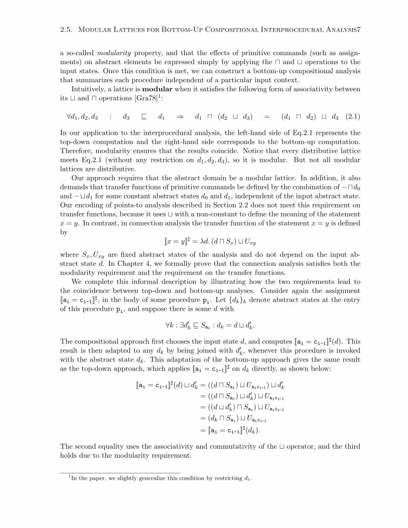
a so-called modularity property, and that the effects of primitive commands (such as assign-ments) on abstract elements be expressed simply by applying the u and t operations to theinput states. Once this condition is met, we can construct a bottom-up compositional analysisthat summarizes each procedure independent of a particular input context.
Intuitively, a lattice is modular when it satisfies the following form of associativity betweenits t and u operations [Gra78]1:
∀d1, d2, d3 : d3 v d1 ⇒ d1 u (d2 t d3) = (d1 u d2) t d3 (2.1)
In our application to the interprocedural analysis, the left-hand side of Eq.2.1 represents thetop-down computation and the right-hand side corresponds to the bottom-up computation.Therefore, modularity ensures that the results coincide. Notice that every distributive latticemeets Eq.2.1 (without any restriction on d1, d2, d3), so it is modular. But not all modularlattices are distributive.
Our approach requires that the abstract domain be a modular lattice. In addition, it alsodemands that transfer functions of primitive commands be defined by the combination of −ud0
and −td1 for some constant abstract states d0 and d1, independent of the input abstract state.Our encoding of points-to analysis described in Section 2.2 does not meet this requirement ontransfer functions, because it uses t with a non-constant to define the meaning of the statementx = y. In contrast, in connection analysis the transfer function of the statement x = y is definedby
[[x = y]]] = λd. (d u Sx) t Uxywhere Sx, Uxy are fixed abstract states of the analysis and do not depend on the input ab-stract state d. In Chapter 4, we formally prove that the connection analysis satisfies both themodularity requirement and the requirement on the transfer functions.
We complete this informal description by illustrating how the two requirements lead tothe coincidence between top-down and bottom-up analyses. Consider again the assignment[[ai = ci-1]]
], in the body of some procedure pi. Let {dk}k denote abstract states at the entryof this procedure pi, and suppose there is some d with
∀k : ∃d′k v Sai : dk = d t d′k.
The compositional approach first chooses the input state d, and computes [[ai = ci-1]]](d). This
result is then adapted to any dk by being joined with d′k, whenever this procedure is invokedwith the abstract state dk. This adaptation of the bottom-up approach gives the same resultas the top-down approach, which applies [[ai = ci-1]]
] on dk directly, as shown below:
[[ai = ci-1]]](d) t d′k = ((d u Sai) t Uaici-1) t d′k
= ((d u Sai) t d′k) t Uaici-1
= ((d t d′k) u Sai) t Uaici-1
= (dk u Sai) t Uaici-1
= [[ai = ci-1]]](dk).
The second equality uses the associativity and commutativity of the t operator, and the thirdholds due to the modularity requirement.
1In the paper, we slightly generalize this condition by restricting d1.

Chapter 3
Preliminaries
In this chapter we introduce the notations used throughout the work.
3.1 Programming Language
Let PComm, G and L be sets of primitive commands, global variables, and local variables,respectively. Also, let PName be a set of procedure names. We use the following symbols torange over these sets:
a, b ∈ PComm, g ∈ G, x, y, z ∈ G ∪ L, p ∈ PName.
We formalize our results for a simple imperative programming language with procedures:
Commands C ::= skip | a | C;C | C + C | C∗ | p()Declarations D ::= proc p() = {var ~x;C}
Programs P ::= var ~g;C | D;P
A program P in our language is a sequence of procedure declarations, followed by a sequence ofdeclarations of global variables and a main command. Commands contain primitive commandsa ∈ PComm, left unspecified, sequential composition C;C ′, nondeterministic choice C + C ′,iteration C∗, and procedure calls p(). We use + and ∗ instead of conditionals and while loopsfor theoretical simplicity: given appropriate primitive commands, conditionals and loops canbe easily defined.
Declarations D give the definitions of procedures. A procedure is comprised of a sequenceof local variables declarations ~x and a command, which we refer to as the procedure’s body.Procedures do not take any parameters or return any values explicitly; values can instead bepassed to and from procedures using global variables. To simplify presentation, we do notconsider mutually recursive procedures in our language; direct recursion is allowed. We denoteby Cbodyp and Lp the body of procedure p and the set of its local variables, respectively.
We assume that L and G are fixed arbitrary finite sets. Also, we consider only well-definedprograms where all the called procedures are defined.
In the rest of the paper, we sometimes need to make use of explicit procedures and localvariables that can be used inside commands, declarations and programs. On these occasions,we express commands, declarations, and programs together with contexts containing possible
8

3.1. Programming Language 9
free variables or procedure names, as shown below:
CΠ,V , DΠ, PΠ,V ,
where Π is a set of procedure names and V is a set of local variables. Note that the contextsdo not say anything about global variables, so any global variable can still appear in C, D andP above.
3.1.1 Standard Semantics
The standard semantics propagates every caller’s context to the callee’s entry point and com-putes the effect of the procedure on each one of them. Formally,
[[p()]]](d) = [[return]]](([[Cbodyp]]] ◦ [[entry]]])(d), d)
where Cbodyp is the body of the procedure p, and
[[entry]]] : D → D, [[return]]] : D ×D → D
are the functions which represent, respectively, entering and returning from a procedure. There-fore, an analysis implemented with the top-down semantics computes a procedure summary forevery calling context.
3.1.2 Relational Collecting Semantics
The semantics of our programming language tracks pairs of memory states 〈σ, σ′〉 coming fromsome unspecified set Σ of memory states. σ is the entry memory state to the procedure of theexecuting command (or if we are executing the main command, the memory state at the startof the program execution), and σ′ is the current memory state. We assume that we are giventhe meaning [[a]] : Σ→ 2Σ of every primitive command, and lift it to sets of pairs ρ ⊆ R = 2Σ×Σ
of memory states of the above form by applying it in a pointwise manner to the current states
[[c]](ρ) = {〈σ, σ′〉 | 〈σ, σ〉 ∈ ρ ∧ σ′ ∈ [[c]](σ)} .
The meaning of composed commands is standard:
[[C1 + C2]](ρ) = [[C1]](ρ) ∪ [[C2]](ρ)
[[C1;C2]](ρ) = [[C2]]([[C1]](ρ))
[[C∗]](ρ) = leastFixλρ′. ρ ∪ [[C]](ρ′).
The effect of procedure invocations is computed using the auxiliary functions entry, return,combine, and ·|G, which we explain below.
[[p()]](ρc) = [[return]]([[Cbodyp]] ◦ [[entry]](ρc), ρc)

10 Chapter 3. Preliminaries
where[[entry]] : R → R
[[entry]](ρc) = {〈σe, σe〉 | σe = σc|G ∧ 〈σc, σc〉 ∈ ρc}
[[return]] : R×R → R[[return]](ρx, ρc) = {combine(σc, σc, σx|G) | 〈σc, σc〉 ∈ ρc
∧ 〈σx, σx〉 ∈ ρx ∧ σc|G = σe|G}
[[combine]] : Σ× Σ× Σ→ R (assumed to be given)( · |G) : Σ→ Σ (assumed to be given)
Function entry computes the relation ρe at the entry to the invoked procedure. It removes theinformation regarding the caller’s local variables from the current states σc coming from thecaller’s relation at the call-site ρc using function ( · |G), which is assumed to be given. Note thatin the computed relation, the entry state and the calling state of the callee are identical.
Function return computes relation ρr, which updates the caller’s current state with theeffect of the callee. The function computes triples 〈σc, σc, σx|G〉 out of pairs of states 〈σc, σc〉and 〈σe, σx〉 from the caller at the time of the call and the callee at the return, such that theglobal part of the caller’s current state matches that of the callee’s entry state. Note that at thetriple, the middle state, σc, contains the values of the caller’s local variables, which the calleecannot modify, and the last state, σx|G, contains the updated state of the global parts of thememory state. Procedure combine combines these two kinds of information and generates theupdated relation at the return site.
Example 1 If we fix the memory states 〈sg, sl, h〉 ∈ Σ to be comprised of environments sg andsl, giving values to global and local variables, respectively, and a heap h, then ( · |G) and combineare defined as
〈sg, sl, h〉|G = 〈sg,⊥, h〉,[[combine]](〈sg, sl, h〉, 〈sg, sl, h〉, 〈s′g,⊥, h′〉)
= (〈sg, sl, h〉, 〈s′g, sl, h′〉).
3.2 Modularity in Lattices
We remind the reader of some standard definitions from the lattice theory:
Definition 2 Let D be a lattice. A pair of elements 〈d0, d1〉 is called modular, denoted byaMb, iff
d v d1 implies that d t (d0 u d1) = (d t d0) u d1
An element d1 is called right-modular if d0Md1 holds for all d0 ∈ D. A lattice D is calledmodular if d0Md1 holds for all d0, d1 ∈ D.
Any distributive lattice is modular. For example, the power set lattice (P (S),⊆) is a modularlattice. Indeed, for every subset d0, d1, d of S,
(d ∩ d1) ∪ (d0 ∩ d1) = (d ∪ d0) ∩ d1 ,
which follows from the distributivity of ∩ over ∪ and implies that if d ⊆ d1, then
d ∪ (d0 ∩ d1) = (d ∪ d0) ∩ d1 .
Chapter 4
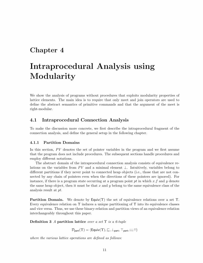
Intraprocedural Analysis usingModularity
We show the analysis of programs without procedures that exploits modularity properties oflattice elements. The main idea is to require that only meet and join operators are used todefine the abstract semantics of primitive commands and that the argument of the meet isright-modular.
4.1 Intraprocedural Connection Analysis
To make the discussion more concrete, we first describe the intraprocedural fragment of theconnection analysis, and define the general setup in the following chapter.
4.1.1 Partition Domains
In this section, PV denotes the set of pointer variables in the program and we first assumethat the program does not include procedures. The subsequent sections handle procedures andemploy different notations.
The abstract domain of the intraprocedural connection analysis consists of equivalence re-lations on the variables from PV and a minimal element ⊥. Intuitively, variables belong todifferent partitions if they never point to connected heap objects (i.e., those that are not con-nected by any chain of pointers even when the directions of these pointers are ignored). Forinstance, if there is a program state occurring at a program point pt in which x.f and y denotethe same heap object, then it must be that x and y belong to the same equivalence class of theanalysis result at pt.
Partition Domain. We denote by Equiv(Υ) the set of equivalence relations over a set Υ.Every equivalence relation on Υ induces a unique partitioning of Υ into its equivalence classesand vice versa. Thus, we use these binary-relation and partition views of an equivalence relationinterchangeably throughout this paper.
Definition 3 A partition lattice over a set Υ is a 6-tuple
Dpart(Υ) = 〈Equiv(Υ),v,⊥part,>part,t,u〉
where the various lattice operations are defined as follows:
11
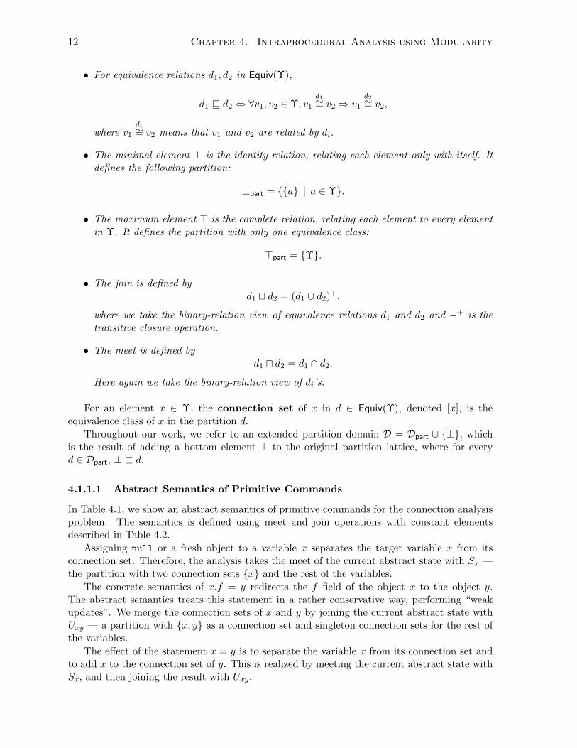
12 Chapter 4. Intraprocedural Analysis using Modularity
• For equivalence relations d1, d2 in Equiv(Υ),
d1 v d2 ⇔ ∀v1, v2 ∈ Υ, v1
d1∼= v2 ⇒ v1
d2∼= v2,
where v1
di∼= v2 means that v1 and v2 are related by di.
• The minimal element ⊥ is the identity relation, relating each element only with itself. Itdefines the following partition:
⊥part = {{a} | a ∈ Υ}.
• The maximum element > is the complete relation, relating each element to every elementin Υ. It defines the partition with only one equivalence class:
>part = {Υ}.
• The join is defined byd1 t d2 = (d1 ∪ d2)+.
where we take the binary-relation view of equivalence relations d1 and d2 and −+ is thetransitive closure operation.
• The meet is defined byd1 u d2 = d1 ∩ d2.
Here again we take the binary-relation view of di’s.
For an element x ∈ Υ, the connection set of x in d ∈ Equiv(Υ), denoted [x], is theequivalence class of x in the partition d.
Throughout our work, we refer to an extended partition domain D = Dpart ∪ {⊥}, whichis the result of adding a bottom element ⊥ to the original partition lattice, where for everyd ∈ Dpart, ⊥ < d.
4.1.1.1 Abstract Semantics of Primitive Commands
In Table 4.1, we show an abstract semantics of primitive commands for the connection analysisproblem. The semantics is defined using meet and join operations with constant elementsdescribed in Table 4.2.
Assigning null or a fresh object to a variable x separates the target variable x from itsconnection set. Therefore, the analysis takes the meet of the current abstract state with Sx —the partition with two connection sets {x} and the rest of the variables.
The concrete semantics of x.f = y redirects the f field of the object x to the object y.The abstract semantics treats this statement in a rather conservative way, performing “weakupdates”. We merge the connection sets of x and y by joining the current abstract state withUxy — a partition with {x, y} as a connection set and singleton connection sets for the rest ofthe variables.
The effect of the statement x = y is to separate the variable x from its connection set andto add x to the connection set of y. This is realized by meeting the current abstract state withSx, and then joining the result with Uxy.

4.2. Conditionally Compositional Intraprocedural Analysis 13
For d = ⊥∀a ∈ AComm[[a]]](d) = d
For d 6= ⊥[[x = null]]](d) = d u Sx
[[y = new]]](d) = d u Sx[[x.f = y]]](d) = d t Uxy
[[x = y]]](d) = (d u Sx) t Uxy[[x = y.f ]]](d) = (d u Sx) t Uxy
Table 4.1: Abstract transfer functions for primitive commands in the connection analysis. InSection 4.1.1.1, x is x and y is y. In Section 5.1, x denotes x′ and y denotes y′.
Uxy = {{x, y}} ∪ {{z} | z ∈ Υ \ {x, y}}Sx = {{x}} ∪ {{z | z ∈ Υ \ {x}}
Table 4.2: Auxiliary constants used in the abstract semantics shown in Table 4.1. Uxy is usedto merge x and y’s connection sets. Sx is used to separate x from its current connection set.
Following [GH96], the effect of the assignment x = y.f is handled in a very conservativemanner, treating y and y.f in the same connection set since the abstraction does not distinguishbetween the objects pointed to by y and y.f . Thus, the same abstract semantics is used forboth x = y.f and x = y.
4.2 Conditionally Compositional Intraprocedural Analysis
Definition 4 (Conditionally Adaptable Functions) Let D be a lattice. A function f :D → D is conditionally adaptable if it has the form
f = λd.((d u dp) t dg)
for some dp, dg ∈ D and the element dp is right-modular. We refer to dp as f ’s meet elementand to dg as f ’s join element.
We focus on static analyses where the transfer function for every primitive command a issome conditionally adaptable function [[a]]]. We denote the meet and join elements of [[a]]] byP [[a]]] and G[[a]]], respectively. For a command C, we denote by P [[C]]] the set of meet elementsof primitive sub-commands occurring in C.
Lemma 5 Let D be a lattice. Let C be a command which does not contain procedure calls. Forevery d1, d2 ∈ D, if d2 v dp for every dp ∈ P [[C]]], then
[[C]]](d1 t d2) = [[C]]](d1) t d2.

14 Chapter 4. Intraprocedural Analysis using Modularity
The proof goes by induction on the structure of commands. The full proof appears in Sec-tion A.3. We present only the most interesting case, which is the one pertaining to primitivecommands. Pick d1, d2 from D. Assume that C is a primitive command a and that d2 v P [[a]]]
. The following derivation shows the lemma:
[[a]]](d1 t d2) = ((d1 t d2) u P [[a]]]) tG[[a]]]
= ((d1 u P [[a]]]) t d2) tG[[a]]]
= ((d1 u P [[a]]]) tG[[a]]]) t d2
= [[a]]](d1) t d2
The first and last equalities hold by definition. The key equality is the second one. It holdsbecause the meet element of a is right-modular and because d2 v P [[a]]]. The third equality isfrom the commutativity and associativity of t.
Lemma 5 can be used to justify compositional summary-based intraprocedural analyses inthe following way: Take a command C and an abstract value d2 such that the conditions of thelemma hold. An analysis that needs to compute the abstract value [[C]]](d1 t d2) can do so bycomputing d = [[C]]](d1), possibly caching (d1, d) in a summary for C, and then adapting theresult by joining d with d2.1
Lemma 6 All the abstract transfer functions of atomic commands in the intraprocedural con-nection analysis are conditionally adaptable.
Recap. The requirement imposed so far by our framework is that the transfer functionsfor primitive commands are conditionally adaptable. Note that our framework justifies onlyconditional intraprocedural summaries; a summary for a command C can be used only whend2 v dp for all dp ∈ P [[C]]]. In contrast, and perhaps counter-intuitively, our framework forthe interprocedural analysis has non-conditional summaries, which do not have a proviso liked2 v P [[C]]]. It achieves this by requiring certain properties of the abstract domain used torecord procedures summaries, which we now describe.
1Interestingly, the notion of condensation in [GRS05] is similar to the implications of Lemma 5 (and tothe frame rule in separation logic) in the sense that the join (or ∗ in separation logic) distributes over thetransfer functions. However, [GRS05] requires the distribution S(a + b) = a + S(b) hold for every two elementsa and b in the domain. Our requirements are less restrictive: In Lemma 5, we require such equality only forelements smaller than or equal to the meet elements of the transfer functions. This is important for handling theconnection analysis in which condensation property does not hold. (In general, the precondition of the equalityin Lemma 5 does not necessarily hold in the intraprocedural case.) (In addition, the method of [GRS05] isdeveloped for domains for logical programs using completion and requires the refined domain to be compatiblewith the projection operator, which is specific to logic programs, and be finitely generated [GRS05, Cor. 4.9].)

Chapter 5
Compositional Analysis usingModularity
In this chapter we define an abstract framework for compositional interprocedural analysis usingmodularity and illustrate the framework using the connection analysis. To make the materialmore accessible, we first formulate the definitions specifically for the connection analysis andexplain them informally in Section 5.1. Then, in Section 5.2, we formalize them for arbitrarydomains. Finally, in Section 5.3, we present a lemma which can be used to apply the theoreticalresult.
The main message is that if we use right-modular elements in a lattice’s subset to summarizethe effects of procedures in a bottom-up manner, we get the coincidence between the results ofthe bottom-up and top-down analyses.
5.1 Compositional Connection Analysis
In Section 5.1.1, we formalize the abstract domains used for interprocedural connection analysis,and in Section 5.1.2 we informally introduce the concept of Triad Domain. In Section 5.1.3we describe the interprocedural top-down triad analyses illustrating the requirements on theconnection analysis. Finally, in Section 5.1.4 we present the interprocedural bottom-up triadconnection analysis, and in Section 5.1.5 we informally describe the coincidence result in theconnection analysis.
In this section we use the program shown in Figure 5.1 as a running example. Each programpoint is marked with a label li. dli denotes the abstract state at li.
5.1.1 Partition Domains for Ternary Relations
We first generalize the abstract domain for the intraprocedural connection analysis describedin Section 4.1.1 to the interprocedural setting.
Recall that the return operation defined in Section 3.1.2 operates on triplets of states. Forthis reason, we use an abstract domain that allows representing ternary relations betweenprogram states. We now formulate this for the connection analysis. We use G and L to denotethe sets of global variables and local variables, respectively. For every global variable g ∈ G, gdenotes the value of g at the entry to a procedure and g′ denotes its current value. The analysiscomputes at every program point a relation between the objects pointed to by global variables
15
16 Chapter 5. Compositional Analysis using Modularity
RX = {{x | x ∈ X}} ∪ {{x} | x ∈ Υ \X}Din = {d ∈ D | d v RG} where RG = {G} ∪ {{x}|x ∈ Υ \ G}Dout = {d ∈ D | d v RG′} where RG = {G′} ∪ {{x}|x ∈ Υ \ G′}Dinout = {d ∈ D | d v RG∪G′} where RG∪G′ = {G ∪ G′} ∪ {{x}|x ∈ Υ \ (G ∪ G′)}Dinoutloc = {d ∈ D | d v RG∪G′∪L′} where RG∪G′∪L′ = {G ∪ G′ ∪ L′} ∪ {{x}|x ∈ Υ \ (G ∪ G′ ∪ L′)}
Table 5.1: Constant projection element RX for an arbitrary set X and the sublattices of D usedby the interprocedural relational analysis. RX is the partition that contains a connection set forall the variables in X and singletons for all the variables in Υ \X. Each one of the sublatticesrepresents connection relations in the current state between objects which were pointed to bylocal or global variables at different stages during the execution. For example, Dinout representsconnection relations in the current state between objects pointed to by global variables in thecurrent state and objects pointed to by global variables at the entry point to the enclosingprocedure.
at the entry to the procedure (represented by G) and the ones pointed to by global variablesand local variables at the current state (represented by G′ and L′, respectively).
For technical reasons, described later, we also use the set G to compute the effect of pro-cedure calls. These sets are used to represent partitions over variables in the same way as inSection 4.1.1. Formally, we define D = Equiv(Υ) ∪ {⊥} in the same way as in Definition 3 ofSection 4.1.1 where Υ = G ∪ G′ ∪ G ∪ L′ and
G′ = {g′ | g ∈ G} G = {g | g ∈ G}G = {g | g ∈ G} L′ = {x′ | x ∈ L}
Remark 1 Formally, the interprocedural connection analysis computes an over-approximationof the relational concrete semantics defined in Section 3.1.2. A Galois connection between theD and a standard (concrete collecting relational) domain for heap manipulating programs isdefined in Section A.2.1.
5.1.2 Triad Partition Domains
In this section, we informally introduce the concept of Triad Domain, which is formalized inSection 5.2.1. Triad domains are used to perform abstract interpretation to represent concretedomains and their concrete semantics as defined in Section 3.1.2. A triad domain is a completelattice which conservatively represents binary and ternary relations (hence the name “triad”)between memory states arising at different program points such as the entry point to the callerprocedure, the call-site, and the current program point.
The analysis uses elements d ∈ D to represent ternary relations when computing procedurereturns. For all other purposes binary relations are used. More specifically, the analysis makesspecial use of the triad sublattices of D defined in Table 5.1, which we now explain.
Each sublattice is used to abstract binary relations between sets of program states, whereeach set is either the set of program states arising at the entry point to the caller procedure, theset of program states arising at the call-site, or the set of program states arising at the currentprogram point. We construct these sublattices by first choosing projection elements dproji fromthe abstract domain D, and then defining the sublattice Di to be the closed interval [⊥, dproji ],
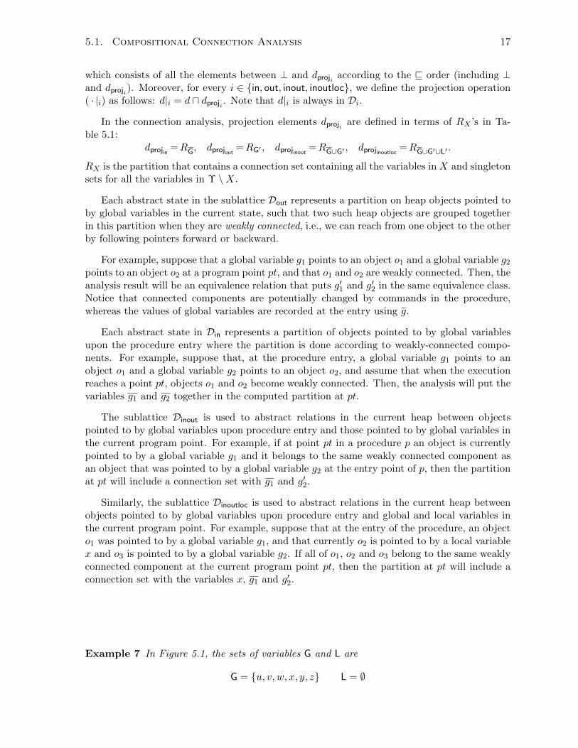
5.1. Compositional Connection Analysis 17
which consists of all the elements between ⊥ and dproji according to the v order (including ⊥and dproji). Moreover, for every i ∈ {in, out, inout, inoutloc}, we define the projection operation( · |i) as follows: d|i = d u dproji . Note that d|i is always in Di.
In the connection analysis, projection elements dproji are defined in terms of RX ’s in Ta-ble 5.1:
dprojin =RG, dprojout =RG′ , dprojinout =RG∪G′ , dprojinoutloc =RG∪G′∪L′ .
RX is the partition that contains a connection set containing all the variables in X and singletonsets for all the variables in Υ \X.
Each abstract state in the sublattice Dout represents a partition on heap objects pointed toby global variables in the current state, such that two such heap objects are grouped togetherin this partition when they are weakly connected, i.e., we can reach from one object to the otherby following pointers forward or backward.
For example, suppose that a global variable g1 points to an object o1 and a global variable g2
points to an object o2 at a program point pt, and that o1 and o2 are weakly connected. Then, theanalysis result will be an equivalence relation that puts g′1 and g′2 in the same equivalence class.Notice that connected components are potentially changed by commands in the procedure,whereas the values of global variables are recorded at the entry using g.
Each abstract state in Din represents a partition of objects pointed to by global variablesupon the procedure entry where the partition is done according to weakly-connected compo-nents. For example, suppose that, at the procedure entry, a global variable g1 points to anobject o1 and a global variable g2 points to an object o2, and assume that when the executionreaches a point pt, objects o1 and o2 become weakly connected. Then, the analysis will put thevariables g1 and g2 together in the computed partition at pt.
The sublattice Dinout is used to abstract relations in the current heap between objectspointed to by global variables upon procedure entry and those pointed to by global variables inthe current program point. For example, if at point pt in a procedure p an object is currentlypointed to by a global variable g1 and it belongs to the same weakly connected component asan object that was pointed to by a global variable g2 at the entry point of p, then the partitionat pt will include a connection set with g1 and g′2.
Similarly, the sublattice Dinoutloc is used to abstract relations in the current heap betweenobjects pointed to by global variables upon procedure entry and global and local variables inthe current program point. For example, suppose that at the entry of the procedure, an objecto1 was pointed to by a global variable g1, and that currently o2 is pointed to by a local variablex and o3 is pointed to by a global variable g2. If all of o1, o2 and o3 belong to the same weaklyconnected component at the current program point pt, then the partition at pt will include aconnection set with the variables x, g1 and g′2.
Example 7 In Figure 5.1, the sets of variables G and L are
G = {u, v, w, x, y, z} L = ∅

18 Chapter 5. Compositional Analysis using Modularity
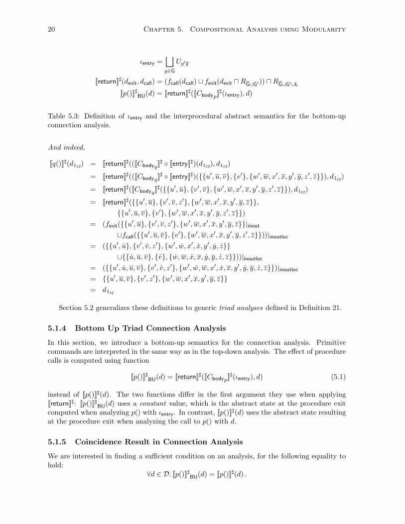
ιentry =⊔g∈G
Ug′g
[[entry]]](d) = (d uRG′) t ιentry[[return]]](dexit, dcall) = (fcall(dcall) t fexit(dexit uRG∪G′)) uRG∪G′∪L
[[p()]]](d) = [[return]]](([[Cbodyp]]] ◦ [[entry]]])(d), d)
Table 5.2: The definition of ιentry and the interprocedural abstract semantics for the top-downconnection analysis. ιentry is the element that represents the identity relation between inputand output, and Cbodyp is the body of the procedure p.
then the projection elements are defined as follows,
dprojout = {{u′, v′, w′, x′, y′, z′}, {u}, {u}, {v}, {v}, {w}, {w}, {x}, {x}, {y}, {y}, {z}, {z}}dprojin = {{u, v, w, x, y, z}, {u′}, {u}, {v′}, {v}, {w′}, {w}, {x′}, {x}, {y′}, {y}, {z′}, {z}}
dprojinout = {{u, u′, v, v′, w, w′, x, x′, y, y′, z, z′}, {u}, {v}, {w}, {x}, {y}, {z}}dprojinoutloc = {{u, u′, v, v′, w, w′, x, x′, y, y′, z, z′}, {u}, {v}, {w}, {x}, {y}, {z}}
Remark 2 For clarity, from now on, in the examples in the figure and formally in the explana-tion we will not show variables g in the abstract states because every g variable is in a singletonset. The only exception is when computing the [[return]]] semantics, where g variables are shownexplicitly.
5.1.3 Interprocedural Top Down Triad Connection Analysis
We describe here the abstract semantics for the top-down interprocedural connection analysis.The intraprocedural semantics is shown in Table 4.1. Notice that there is a minor differencebetween the semantics of primitive commands for the intraprocedural connection analysis de-fined in Section 4.1.1.1 and for the analysis in this section. In the analysis without procedureswe use x, whereas in the analysis of this section we use x′.
The interprocedural effect for the connection analysis is defined in Table 5.2. Again, werefer to the auxiliary constant elements RX for a set X defined in Table 5.1.
When a procedure is entered, local variables of the procedure and all the global variablesg at the entry to the procedure are initialized to null. This is realized by applying the meetoperation with auxiliary variable RG′ . Then, each of the g is initialized with the current variablevalue g′ using ιentry. The ιentry element denotes a particular state that abstracts the identityrelation between input and output states. In the connection analysis, it is defined by a partitioncontaining {g, g′} connection sets for all global variables g. Intuitively, this stores the currentvalue of variable g into g, by representing the case where the object currently pointed to by gis in the same weakly connected component as the object that was pointed to by g at the entrypoint of the procedure.
Example 8 In Figure 5.1, dl13 is the abstract state at l13, q’s call-site and dl15 is the abstract

5.1. Compositional Connection Analysis 19
state at l15, the entry point of q.
dl13 = {{u′, u, v}, {v′}, {w′, w, x′, x, y′, y, z′, z}}
We compute [[entry]]](dl13) in two stages. First, we project dl13 into Dout
dl13 |out = dl13 uRG′
= dl13 u {G′, {{x} | x 6∈ G′}}= {{u′, u, v}, {v′}, {w′, w, x′, x, y′, y, z′, z}} u {G′, {{x} | x 6∈ G′}}= {{u′}, {u}, {v′}, {v}, {w′, x′, y′, z′}, {w}, {x}, {y}, {z}}
We then compute the join of dl13 |out with ιentry.
[[entry]]](dl13) = dl13 |out t ιentry= dl13 |out t {{u′, u}, {v′, v}, {w′, w}, {x′, x}, {y′, y}, {z′, z}}= {{u′, u}, {v′, v}, {w′, w, x′, x, y′, y, z′, z}} = dl15 .
The effect of returning from a procedure is more complex. It takes two inputs: dcall, whichrepresents the partition at the call-site, and dexit, which represents the partition at the exitfrom the procedure. The meet operation of dexit with RG∪G′ emulates the nullification of localvariables of the procedure.
The computed abstract values emulate the composition of the input-output relation of thecall-site with that of the return-site. Variables of the form g are used to implement a naturaljoin operation for composing these relations. fcall(dcall) renames global variables from g′ to gand fexit(dexit) renames global variables from g to g to allow natural join. Intuitively, the oldvalues g of the callee at the exit-site are matched with the current values g′ of the caller at thecall-site.
The last meet operation represents the nullification of the temporary values g of the globalvariables.
Example 9 In Figure 5.1, dl13 is the abstract state at l13, q’s call-site, while dl14 is the abstractstate after q’s execution, i.e.
dl14 = [[q()]]](dl13)
20 Chapter 5. Compositional Analysis using Modularity
ιentry =⊔g∈G
Ug′g
[[return]]](dexit, dcall) = (fcall(dcall) t fexit(dexit uRG∪G′)) uRG∪G′∪L
[[p()]]]BU(d) = [[return]]]([[Cbodyp]]](ιentry), d)
Table 5.3: Definition of ιentry and the interprocedural abstract semantics for the bottom-upconnection analysis.
And indeed,
[[q()]]](dl13) = [[return]]](([[Cbodyq]]] ◦ [[entry]]])(dl13), dl13)
= [[return]]](([[Cbodyq]]] ◦ [[entry]]])({{u′, u, v}, {v′}, {w′, w, x′, x, y′, y, z′, z}}), dl13)
= [[return]]]([[Cbodyq]]]({{u′, u}, {v′, v}, {w′, w, x′, x, y′, y, z′, z}}), dl13)
= [[return]]]({{u′, u}, {v′, v, z′}, {w′, w, x′, x, y′, y, z}},{{u′, u, v}, {v′}, {w′, w, x′, x, y′, y, z′, z}})
= (fexit({{u′, u}, {v′, v, z′}, {w′, w, x′, x, y′, y, z}}|inouttfcall({{u′, u, v}, {v′}, {w′, w, x′, x, y′, y, z′, z}}))|inoutloc
= ({{u′, u}, {v′, v, z′}, {w′, w, x′, x, y′, y, z}}t{{u, u, v}, {v}, {w, w, x, x, y, y, z, z}}))|inoutloc
= ({{u′, u, u, v}, {v′, v, z′}, {w′, w, w, x′, x, x, y′, y, y, z, z}})|inoutloc= {{u′, u, v}, {v′, z′}, {w′, w, x′, x, y′, y, z}}= dl14
Section 5.2 generalizes these definitions to generic triad analyses defined in Definition 21.
5.1.4 Bottom Up Triad Connection Analysis
In this section, we introduce a bottom-up semantics for the connection analysis. Primitivecommands are interpreted in the same way as in the top-down analysis. The effect of procedurecalls is computed using function
[[p()]]]BU(d) = [[return]]]([[Cbodyp]]](ιentry), d) (5.1)
instead of [[p()]]](d). The two functions differ in the first argument they use when applying[[return]]]: [[p()]]]BU(d) uses a constant value, which is the abstract state at the procedure exitcomputed when analyzing p() with ιentry. In contrast, [[p()]]](d) uses the abstract state resultingat the procedure exit when analyzing the call to p() with d.
5.1.5 Coincidence Result in Connection Analysis
We are interested in finding a sufficient condition on an analysis, for the following equality tohold:
∀d ∈ D. [[p()]]]BU(d) = [[p()]]](d) .
5.1. Compositional Connection Analysis 21
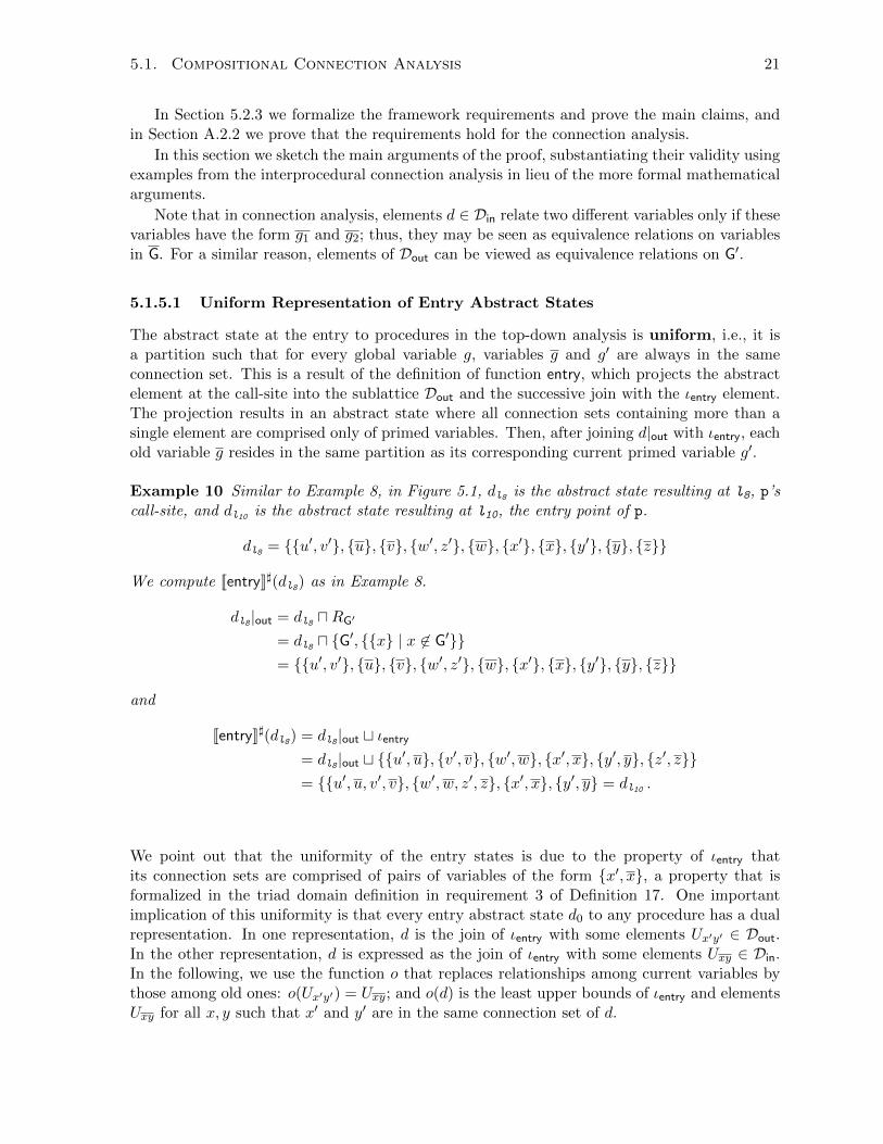
In Section 5.2.3 we formalize the framework requirements and prove the main claims, andin Section A.2.2 we prove that the requirements hold for the connection analysis.
In this section we sketch the main arguments of the proof, substantiating their validity usingexamples from the interprocedural connection analysis in lieu of the more formal mathematicalarguments.
Note that in connection analysis, elements d ∈ Din relate two different variables only if thesevariables have the form g1 and g2; thus, they may be seen as equivalence relations on variablesin G. For a similar reason, elements of Dout can be viewed as equivalence relations on G′.
5.1.5.1 Uniform Representation of Entry Abstract States
The abstract state at the entry to procedures in the top-down analysis is uniform, i.e., it isa partition such that for every global variable g, variables g and g′ are always in the sameconnection set. This is a result of the definition of function entry, which projects the abstractelement at the call-site into the sublattice Dout and the successive join with the ιentry element.The projection results in an abstract state where all connection sets containing more than asingle element are comprised only of primed variables. Then, after joining d|out with ιentry, eachold variable g resides in the same partition as its corresponding current primed variable g′.
Example 10 Similar to Example 8, in Figure 5.1, dl8 is the abstract state resulting at l8, p’scall-site, and dl10 is the abstract state resulting at l10, the entry point of p.
dl8 = {{u′, v′}, {u}, {v}, {w′, z′}, {w}, {x′}, {x}, {y′}, {y}, {z}}
We compute [[entry]]](dl8) as in Example 8.
dl8 |out = dl8 uRG′
= dl8 u {G′, {{x} | x 6∈ G′}}= {{u′, v′}, {u}, {v}, {w′, z′}, {w}, {x′}, {x}, {y′}, {y}, {z}}
and
[[entry]]](dl8) = dl8 |out t ιentry= dl8 |out t {{u′, u}, {v′, v}, {w′, w}, {x′, x}, {y′, y}, {z′, z}}= {{u′, u, v′, v}, {w′, w, z′, z}, {x′, x}, {y′, y} = dl10 .
We point out that the uniformity of the entry states is due to the property of ιentry thatits connection sets are comprised of pairs of variables of the form {x′, x}, a property that isformalized in the triad domain definition in requirement 3 of Definition 17. One importantimplication of this uniformity is that every entry abstract state d0 to any procedure has a dualrepresentation. In one representation, d is the join of ιentry with some elements Ux′y′ ∈ Dout.In the other representation, d is expressed as the join of ιentry with some elements Uxy ∈ Din.In the following, we use the function o that replaces relationships among current variables bythose among old ones: o(Ux′y′) = Uxy; and o(d) is the least upper bounds of ιentry and elementsUxy for all x, y such that x′ and y′ are in the same connection set of d.
22 Chapter 5. Compositional Analysis using Modularity
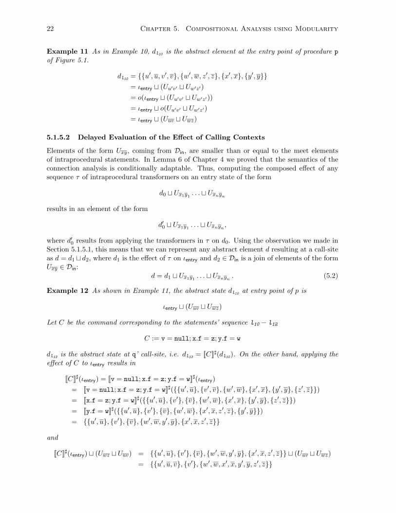
Example 11 As in Example 10, dl10 is the abstract element at the entry point of procedure p
of Figure 5.1.
dl10 = {{u′, u, v′, v}, {w′, w, z′, z}, {x′, x}, {y′, y}}= ιentry t (Uu′v′ t Uw′z′)= o(ιentry t (Uu′v′ t Uw′z′))= ιentry t o(Uu′v′ t Uw′z′)= ιentry t (Uuv t Uwz)
5.1.5.2 Delayed Evaluation of the Effect of Calling Contexts
Elements of the form Uxy, coming from Din, are smaller than or equal to the meet elementsof intraprocedural statements. In Lemma 6 of Chapter 4 we proved that the semantics of theconnection analysis is conditionally adaptable. Thus, computing the composed effect of anysequence τ of intraprocedural transformers on an entry state of the form
d0 t Ux1y1 . . . t Uxnyn
results in an element of the form
d′0 t Ux1y1 . . . t Uxnyn ,
where d′0 results from applying the transformers in τ on d0. Using the observation we made inSection 5.1.5.1, this means that we can represent any abstract element d resulting at a call-siteas d = d1 t d2, where d1 is the effect of τ on ιentry and d2 ∈ Din is a join of elements of the formUxy ∈ Din:
d = d1 t Ux1y1 . . . t Uxnyn . (5.2)
Example 12 As shown in Example 11, the abstract state dl10 at entry point of p is
ιentry t (Uuv t Uwz)
Let C be the command corresponding to the statements’ sequence l10 − l12
C := v = null; x.f = z; y.f = w
dl13 is the abstract state at q’ call-site, i.e. dl13 = [[C]]](dl10). On the other hand, applying theeffect of C to ιentry results in
[[C]]](ιentry) = [[v = null; x.f = z; y.f = w]]](ιentry)
= [[v = null; x.f = z; y.f = w]]]({{u′, u}, {v′, v}, {w′, w}, {x′, x}, {y′, y}, {z′, z}})= [[x.f = z; y.f = w]]]({{u′, u}, {v′}, {v}, {w′, w}, {x′, x}, {y′, y}, {z′, z}})= [[y.f = w]]]({{u′, u}, {v′}, {v}, {w′, w}, {x′, x, z′, z}, {y′, y}})= {{u′, u}, {v′}, {v}, {w′, w, y′, y}, {x′, x, z′, z}}
and
[[C]]](ιentry) t (Uwz t Uuv) = {{u′, u}, {v′}, {v}, {w′, w, y′, y}, {x′, x, z′, z}} t (Uuv t Uwz)= {{u′, u, v}, {v′}, {w′, w, x′, x, y′, y, z′, z}}

5.1. Compositional Connection Analysis 23
which is equal to dl13.
5.1.5.3 Counterpart Representation for Calling Contexts
Because of the previous reasoning, we can now assume that any abstract value at the call-siteto a procedure p() is of the form d1 t d3, where d3 ∈ Din and it is a join of elements of formUxy.
For each Uxy, the entry state resulting from analyzing p() when the calling context is d1tUxyis either identical to the one resulting from d1 or can be obtained from d1 by merging two ofits connection sets. Furthermore, the need to merge occurs only if there are variables w′ and z′
such that w′ and x are in one of the connection sets and z′ and y are in another. This meansthat the effect of Uxy on the entry state can be expressed via primed variables:
d1 t Uxy = d1 t Uw′z′ .
This implies that if the abstract state at the call-site is d1td3, then there is an element d′3 ∈ Dout
such that(d1 t d3)|out = d1|out t d′3 (5.3)
We refer to the element d′3 ∈ Dout, which can be used to represent the effect of d3 ∈ Din at the
call-site as d3’s counterpart, and denote it by d3.
In Definition 17 of Section 5.2.1 we introduce the concept of context-adaptable which for-malizes this property.
Example 13 Letd1 = {{u′, u}, {v′}, {v}, {w′, w, y′, y}, {x′, x, z′, z}}
andd3 = Uwz
Joining d1 with Uwz causes connection sets [w] and [z] to be merged, and, consequently, [y′] and[x′] are merged, since [y′] = [w] and [x′] = [z] . Therefore,
(d1 t d3)|out = (d1 t Ux′z′)|out
and in this case d3 = Ux′z′.
5.1.5.4 Representing Entry States with Counterparts
The above facts imply that we can represent an abstract state d at the call-site as
d = d1 t d3 t d4, (5.4)
where d3, d4 ∈ Din. d3 is a join of the elements of the form Uxy such that x and y reside in d1 indifferent partitions, which also contain current (primed) variables, and thus possibly affect theentry state; d4 is a join of all the other elements Uxy ∈ Din, which are needed to represent d inthis form, but either x or y resides in the same partition in d1 or one of them is in a partitioncontaining only old variables. Note that, as explained in the previous paragraph, there is anelement d′3 = d3 that joins elements of the form Ux′y′ such that
d1 t d3 = d1 t d′3. (5.5)

24 Chapter 5. Compositional Analysis using Modularity
and therefored = d1 t d3 t d4 = d1 t d′3 t d4 . (5.6)
Thus, after applying the entry’s semantics, we get that abstract states at the entry point ofprocedure are always of the form
(d1 t d′3)|out t ιentrywhere d′3 represents the effect of d4 t d3 on partitions containing current variables g′ in d1.Because Ux′y′ v RG′ , and d′3 joins elements of form Ux′y′ , we get from the modularity of thelattice that
(d1 t d′3)|out t ιentry = (d1|out t d′3) t ιentryThis implies that every state d0 at an entry point to a procedure is of the following form:
d0 = ιentry t (Ux′y′ . . . t Ux′ly′l)︸ ︷︷ ︸d1|out
t (Ux′l+1y′l+1
. . . t Ux′ny′n)︸ ︷︷ ︸d′3
.
Using the dual representation of entry state, we get that
ιentry t Ux′1y′1 . . . t Ux′ny′n = ιentry t o(Ux′1y′1 . . . t Ux′ny′n)
Finally, we get that every state d0 at an entry point to a procedure is of the form
d0 = ιentry t Ux1y1 t . . . t Uxnyn (5.7)
Example 14 We showed in Example 12 that the abstract state at the call-site of procedure q
isdl13 = d1 t d2
whered1 = {{u′, u}, {v′}, {v}, {w′, w, y′, y}, {x′, x, z′, z}}
andd2 = Uuv t Uwz
In Example 13 we showed that Uwz affects current variables and Uwz = Ux′y′. In contrast,joining the result with Uuv has no effect on relations between current variables, because theconnection set [v] does not contain a current variable. Therefore, in this case,
d3 = Uwz
d′3 = Ux′y′
d4 = Uuv
and clearlyd1 t d3 t d4 = d1 t d′3 t d4
Let’s then look at dl15, the abstract element at procedure q’s entry point.
dl15 = {{u′, u}, {v′, v}, {w′, w, x′, x, y′, y, z′, z}}= ιentry t {{u′}, {u}, {v′}, {v}, {w′, y′}, {w}, {x′, z′}, {x}, {y}, {z}} t Uwz= ιentry t d1|out t d′3

5.1. Compositional Connection Analysis 25
5.1.5.5 Putting It All Together
Based on the above arguments, we now show that the interprocedural connection analysis canbe done compositionally. Intuitively, the effect of the caller’s calling context can be carriedover procedure invocations. Alternatively, the effect of the callee on the caller’s context can beadapted unconditionally for different caller’s calling contexts.
We sketch here an outline of the proof of Lemma 23 in Section 5.2.3 for case C = p()using the connection analysis domain. The proof goes by induction on the structure of theprogram. In Eq.5.4 we showed that every abstract value that arises at the call-site is of theform d1 t d3 t d4, where d3, d4 ∈ Din.
Thus, we show that
[[C]]](d1 t d3 t d4) = [[C]]](d1) t d3 t d4 . (5.8)
Say we want to compute the effect of invoking p() on abstract state d according to thetop-down abstract semantics.
[[p()]]](d) = [[return]]]((
([[Cbodyp]]] ◦ [[entry]]])(d)
), d)
First, let’s compute the first argument to [[return]]].
([[Cbodyp]]] ◦ [[entry]]])(d)
= [[Cbodyp]]]([[entry]]](d1 t d3 t d4))
= [[Cbodyp]]](((d1 t d3 t d4)|out) t ιentry)
= [[Cbodyp]]](((d1 t d3)|out) t ιentry)
= [[Cbodyp]]]((d1)|out t d′3 t ιentry)
= [[Cbodyp]]]((d1)|out t o(d′3) t ιentry)
= [[Cbodyp]]]((d1)|out t ιentry) t o(d′3) (5.9)
The first equalities are mere substitutions based on observations we made before. The last onecomes from the induction assumption.
When applying the return semantics, we first compute the natural join and then remove thetemporary variables. Therefore, we get
(fcall(d1 t d3 t d4) t fexit([[Cbodyp]]]((d1)|out t ιentry) t o(d′3)))|inoutloc
Let’s first compute the result of the inner parentheses.
fcall(d1 t d3 t d4) t fexit([[Cbodyp]]]((d1)|out t ιentry) t o(d′3))
= fcall(d1 t d′3 t d4) t fexit([[Cbodyp]]]((d1)|out t ιentry) t o(d′3))
= fcall(d′3) t fcall(d1 t d4) t
fexit(o(d′3)) t fexit([[Cbodyp]]
]((d1)|out t ιentry)) (5.10)
The first equality is by the definition of d′3 and the last equality is by the isomorphism ofthe renaming operations fcall and fexit.

26 Chapter 5. Compositional Analysis using Modularity
Note, among the join arguments, fexit(o(d′3)) and fcall(d
′3). Let’s look at the first element.
o(d′3) replaces all the occurrences of Ux′y′ in d′3 with Uxy. fexit replaces all the occurrences ofUxy in o(d′3) with Uxy. Thus, the first element is
Ux1y1 t . . . t Uxnyn
which is the result of replacing in d′3 all the occurrences of Ux′y′ with Uxy. Let’s look now atthe second element. fexit replaces all occurrences of Ux′y′ in d′3 with Uxy. Thus, also the secondelement is
Ux1y1 t . . . t UxnynThus, we get that
(5.10) = fcall(d′3) t fcall(d1 t d4) t fexit([[Cbodyp]]
]((d1)|out t ιentry))
Moreover, fcall is isomorphic and by Eq.5.6
= fcall(d3 t d1 t d4) t fexit([[Cbodyp]]]((d1)|out t ιentry))
Remember (Eq.5.2) that d3 and d4 are both of form
Ux1y1 t . . . t Uxnyn
and that fcall(d) only replaces g′ occurrences in d; thus
= fcall(Ux1y1 t . . . t Uxnyn) = Ux1y1 t . . . t Uxnyn
Finally, we get= fcall(d1) t fexit([[Cbodyp]]
]((d1)|out t ιentry) t (d3 t d4)
= [[p()]]](d1) t d3 t d4
Example 15 Recall that in Example 12 we showed that
dl13 = {{u′, u}, {v′}, {v}, {w′, w, y′, y}, {x′, x, z′, z}} t (Uuv t Uwz)
Letd1 = {{u′, u}, {v′}, {v}, {w′, w, y′, y}, {x′, x, z′, z}}
andd2 = Uuv t Uwz

5.1. Compositional Connection Analysis 27
Thus, dl13 = d1 t d2 where d2 ∈ Din. Let’s now apply [[q()]]] to d1
[[q()]]](d1) = [[return]]](([[Cbodyq]]] ◦ [[entry]]])(d1), d1)
= [[return]]](([[Cbodyq]]] ◦ [[entry]]])({{u′, u}, {v′}, {v}, {w′, w, y′, y}, {x′, x, z′, z}}), d1)
= [[return]]]([[Cbodyq]]]({{u′, u}, {v′, v}, {w′, w, y′, y}, {x′, x, z′, z}}), d1)
= [[return]]]({{u′, u}, {v′, v, z′}, {w′, w, y′, y}, {x′, x, z}},{{u′, u}, {v′}, {v}, {w′, w, y′, y}, {x′, x, z′, z}})
= (fexit({{u′, u}, {v′, v, z′}, {w′, w, y′, y}, {x′, x, z}}|inouttfcall({{u′, u}, {v′}, {v}, {w′, w, y′, y}, {x′, x, z′, z}}))inoutloc
= ({{u′, u}, {v′, v, z′}, {w′, w, y′, y}, {x′, x, z}}t{{u, u}, {v}, {v}, {w, w, y, y}, {x, x, z, z}})inoutloc
= ({{u′, u, u}, {v′, v, z′}, {v}, {w′, w, w, y′, y, y}, {x′, x, x, z, z}})inoutloc= {{u′, u}, {v′, z′}, {v}, {w′, w, y′, y}, {x′, x, z}}
Then
[[q()]]](d1) t d2 = {{u′, u}, {v′, z′}, {v}}, {w′, w, y′, y}, {x′, x, z}} t (Uuv t Uwz)= {{u′, u, v}, {z′, v′}, {w′, w, x′, x, y′, y, z}}= dl14 = [[q()]]](dl13) = [[q()]]](d1 t d2)
5.1.5.6 Precision Coincidence
We combine the observations we made to informally show the coincidence result between thetop-down and the bottom-up semantics, which is formally proven in Theorem 22 of Section 5.2.3.According to Eq.5.4, every state d at a call-site can be represented as d = d1 t d3 t d4, whered3, d4 ∈ Din
[[p()]]](d) = [[return]]]([[Cbodyp ]]]([[entry]]](d)), d)
= [[return]]]([[Cbodyp ]]](d1|out t ιentry t d′3), d)
= [[return]]]([[Cbodyp ]]](ιentry t o(d1|out) t o(d′3)), d) .
We showed that for every d = d1 t d3 t d4, such that d3, d4 ∈ Din and command C,
[[C]]](d1 t d3 t d4) = [[C]]](d1) t d3 t d4 .
Therefore, since o(d′3), o(d1|out) ∈ Din,
= [[return]]]([[Cbodyp ]]](ιentry) t o(d1|out) t o(d′3), d1 t d3 t d4)
By Eq.5.6,d1 t d3 t d4 = d1 t d′3 t d4
Thus, we can remove o(d′3) because fexit(o(d′3)) is redundant in the natural join. Using a similar
reasoning, we can remove fexit(o(d1|out)), since fcall(d1|out) v fcall(d1).

28 Chapter 5. Compositional Analysis using Modularity
Finally,
= [[return]]]([[Cbodyp ]]](ιentry), d1 t d3 t d4) = [[p()]]]BU(d)
Example 16 Let’s now use the bottom-up semantics to compute the result of applying p() todl8. We start by computing [[Cbodyp ]]](ιentry)
[[Cbodyp ]]](ιentry) = [[Cbodyp ]]]({{u′, u}, {v′, v}, {w′, w}, {x′, x}, {y′, y}, {z′, z}})= {{u′, u}, {v}, {v′, z′}, {w′, w, y′, y}, {x′, x, z}}
Then,
[[p()]]]BU(dl8)
= [[return]]]([[Cbodyp ]]](ιentry), dl8)
= (fexit({{u′, u}, {v′, z′}, {v}, {w′, w, y′, y}, {x′, x, z}}) t fcall(dl8 |inout))|inoutloc= (fexit({{u′, u}, {v′, z′}, {v}, {w′, w, y′, y}, {x′, x, z}})
tfcall({{u′, v′}, {u}, {v}, {w}, {x′}, {x}, {y′}, {y}, {w′, z′}, {z}}|inout))|inoutloc= (fexit({{u′, u}, {v′, z′}, {v}, {w′, w, y′, y}, {x′, x, z}})
tfcall({{u′, v′}, {u}, {v}, {w}, {x′}, {x}, {y′}, {y}, {w′, z′}, {z}}))|inoutloc= ({{u′, u}, {v′, z′}, {v}, {w′, w, y′, y}, {x′, x, z}}
t{{u, v}, {u}, {v}, {w}, {x}, {x}, {y}, {y}, {w, z}, {z}})|inoutloc= ({{u′, u, v}, {v′, z′}, {u}, {v}, {w′, w, x′, x, y′, y, z}, {w}, {x}, {y}, {z}})|inoutloc= {{u′}, {v′, z′}, {u}, {v}, {w′, x′, y′}, {w}, {x}, {y}, {z}}= dl9 = [[p()]]](dl8)
5.2 Compositional Analysis
In this section we give formal definitions and proofs of what we informally explained in Sec-tion 5.1.
5.2.1 Triad Domains
As previously mentioned, triad domains are used to perform abstract interpretation of theconcrete domains and their concrete semantics as defined in Section 3.1.2. This is achievedusing isomorphic sublattices of the domain, where each lattice is used to represent properties ofsets of states at different program points and requiring certain properties on the isomorphisms.
Definition 17 A complete lattice D is a Triad Domain if
1. There exist right-modular elements
dprojindprojout , dprojtmp, dprojloc , dprojinout , dprojinoutloc ∈ D
2. There exist three isomorphism functions fcall, fexit, finout,
fi : D → D for i ∈ {call, exit, inout}
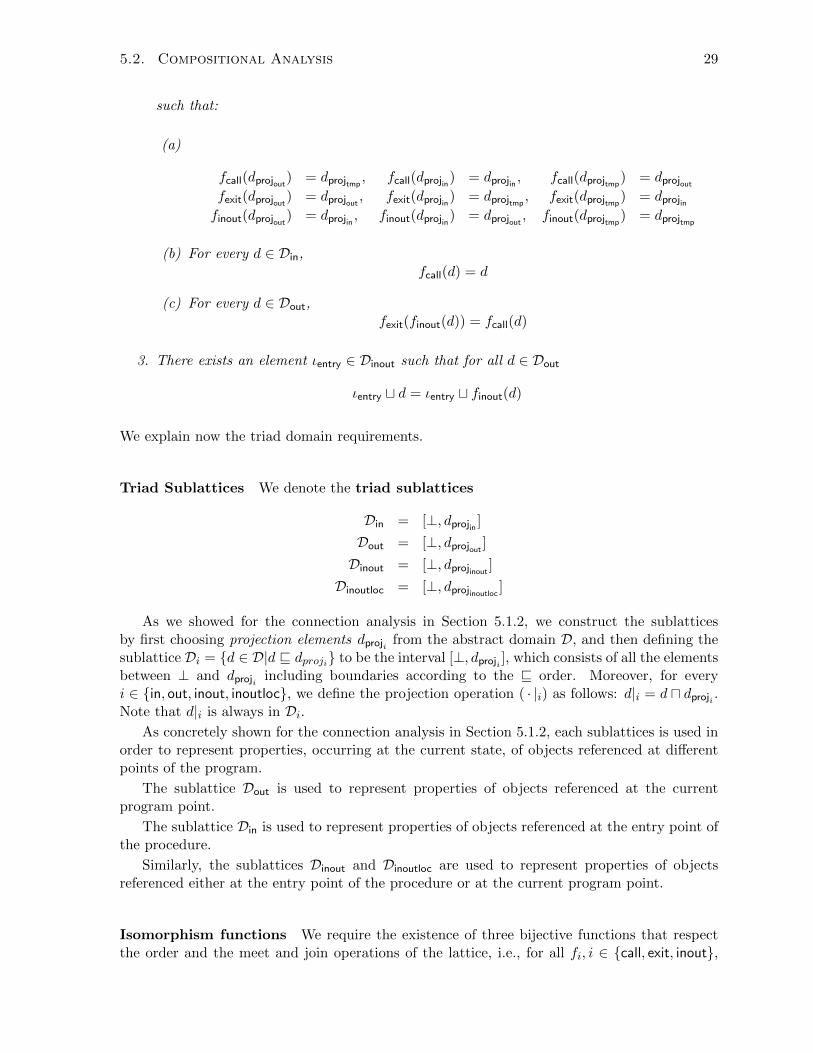
5.2. Compositional Analysis 29
such that:
(a)
fcall(dprojout) = dprojtmp, fcall(dprojin) = dprojin , fcall(dprojtmp
) = dprojoutfexit(dprojout) = dprojout , fexit(dprojin) = dprojtmp
, fexit(dprojtmp) = dprojin
finout(dprojout) = dprojin , finout(dprojin) = dprojout , finout(dprojtmp) = dprojtmp
(b) For every d ∈ Din,fcall(d) = d
(c) For every d ∈ Dout,fexit(finout(d)) = fcall(d)
3. There exists an element ιentry ∈ Dinout such that for all d ∈ Dout
ιentry t d = ιentry t finout(d)
We explain now the triad domain requirements.
Triad Sublattices We denote the triad sublattices
Din = [⊥, dprojin ]Dout = [⊥, dprojout ]Dinout = [⊥, dprojinout ]Dinoutloc = [⊥, dprojinoutloc ]
As we showed for the connection analysis in Section 5.1.2, we construct the sublatticesby first choosing projection elements dproji from the abstract domain D, and then defining thesublattice Di = {d ∈ D|d v dproji} to be the interval [⊥, dproji ], which consists of all the elementsbetween ⊥ and dproji including boundaries according to the v order. Moreover, for everyi ∈ {in, out, inout, inoutloc}, we define the projection operation ( · |i) as follows: d|i = d u dproji .Note that d|i is always in Di.
As concretely shown for the connection analysis in Section 5.1.2, each sublattices is used inorder to represent properties, occurring at the current state, of objects referenced at differentpoints of the program.
The sublattice Dout is used to represent properties of objects referenced at the currentprogram point.
The sublattice Din is used to represent properties of objects referenced at the entry point ofthe procedure.
Similarly, the sublattices Dinout and Dinoutloc are used to represent properties of objectsreferenced either at the entry point of the procedure or at the current program point.
Isomorphism functions We require the existence of three bijective functions that respectthe order and the meet and join operations of the lattice, i.e., for all fi, i ∈ {call, exit, inout},
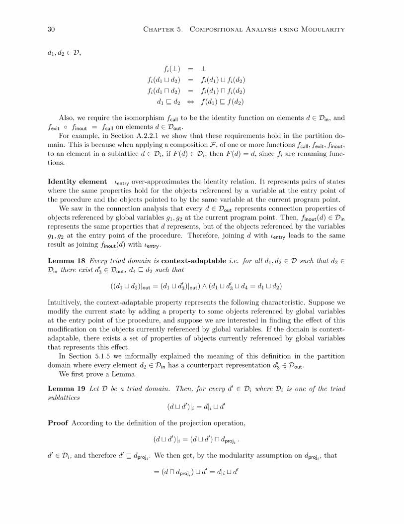
30 Chapter 5. Compositional Analysis using Modularity
d1, d2 ∈ D,
fi(⊥) = ⊥fi(d1 t d2) = fi(d1) t fi(d2)
fi(d1 u d2) = fi(d1) u fi(d2)
d1 v d2 ⇔ f(d1) v f(d2)
Also, we require the isomorphism fcall to be the identity function on elements d ∈ Din, andfexit ◦ finout = fcall on elements d ∈ Dout.
For example, in Section A.2.2.1 we show that these requirements hold in the partition do-main. This is because when applying a composition F , of one or more functions fcall, fexit, finout,to an element in a sublattice d ∈ Di, if F (d) ∈ Di, then F (d) = d, since fi are renaming func-tions.
Identity element ιentry over-approximates the identity relation. It represents pairs of stateswhere the same properties hold for the objects referenced by a variable at the entry point ofthe procedure and the objects pointed to by the same variable at the current program point.
We saw in the connection analysis that every d ∈ Dout represents connection properties ofobjects referenced by global variables g1, g2 at the current program point. Then, finout(d) ∈ Din
represents the same properties that d represents, but of the objects referenced by the variablesg1, g2 at the entry point of the procedure. Therefore, joining d with ιentry leads to the sameresult as joining finout(d) with ιentry.
Lemma 18 Every triad domain is context-adaptable i.e. for all d1, d2 ∈ D such that d2 ∈Din there exist d′3 ∈ Dout, d4 v d2 such that
((d1 t d2)|out = (d1 t d′3)|out) ∧ (d1 t d′3 t d4 = d1 t d2)
Intuitively, the context-adaptable property represents the following characteristic. Suppose wemodify the current state by adding a property to some objects referenced by global variablesat the entry point of the procedure, and suppose we are interested in finding the effect of thismodification on the objects currently referenced by global variables. If the domain is context-adaptable, there exists a set of properties of objects currently referenced by global variablesthat represents this effect.
In Section 5.1.5 we informally explained the meaning of this definition in the partitiondomain where every element d2 ∈ Din has a counterpart representation d′3 ∈ Dout.
We first prove a Lemma.
Lemma 19 Let D be a triad domain. Then, for every d′ ∈ Di where Di is one of the triadsublattices
(d t d′)|i = d|i t d′
Proof According to the definition of the projection operation,
(d t d′)|i = (d t d′) u dproji .
d′ ∈ Di, and therefore d′ v dproji . We then get, by the modularity assumption on dproji , that
= (d u dproji) t d′ = d|i t d′
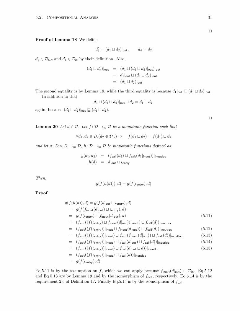
5.2. Compositional Analysis 31
2
Proof of Lemma 18 We define
d′3 = (d1 t d2)|out, d4 = d2
d′3 ∈ Dout and d4 ∈ Din by their definition. Also,
(d1 t d′3)|out = (d1 t (d1 t d2)|out)|out= d1|out t (d1 t d2)|out= (d1 t d2)|out
The second equality is by Lemma 19, while the third equality is because d1|out v (d1 t d2)|out.In addition to that
d1 t (d1 t d2)|out t d2 = d1 t d2,
again, because (d1 t d2)|out v (d1 t d2).
2
Lemma 20 Let d ∈ D. Let f : D →m D be a monotonic function such that
∀d1, d2 ∈ D.(d2 ∈ Din)⇒ f(d1 t d2) = f(d1) t d2
and let g : D ×D →m D, h : D →m D be monotonic functions defined as:
g(d1, d2) = (fcall(d2) t fexit(d1|inout))|inoutloch(d) = d|out t ιentry
Then,g(f(h(d))), d) = g(f(ιentry), d)
Proof
g(f(h(d)), d) = g(f(d|out t ιentry), d)
= g(f(finout(d|out) t ιentry), d)
= g(f(ιentry) t finout(d|out), d) (5.11)
= (fexit((f(ιentry) t finout(d|out))|inout) t fcall(d))|inoutloc= (fexit((f(ιentry))|inout t finout(d|out)) t fcall(d))|inoutloc (5.12)
= (fexit((f(ιentry))|inout) t fexit(finout(d|out)) t fcall(d))|inoutloc (5.13)
= (fexit((f(ιentry))|inout) t fcall(d|out) t fcall(d))|inoutloc (5.14)
= (fexit((f(ιentry))|inout) t fcall(d|out t d))|inoutloc (5.15)
= (fexit((f(ιentry))|inout) t fcall(d))|inoutloc= g(f(ιentry), d)
Eq.5.11 is by the assumption on f , which we can apply because finout(d|out) ∈ Din. Eq.5.12and Eq.5.13 are by Lemma 19 and by the isomorphism of fexit, respectively. Eq.5.14 is by therequirement 2.c of Definition 17. Finally Eq.5.15 is by the isomorphism of fcall.

32 Chapter 5. Compositional Analysis using Modularity
[[CΠ,V ]]] : [[Π]]] →m F[[a]]](µ, d) = trans(a)(d)
[[C1;C2]]](µ, d) = [[C2]]](µ, ([[C1]]](µ, d))[[C1 + C2]]](µ, d) = ([[C1]]](µ, d)) t ([[C2]]](µ, d))
[[C∗]]](µ, d) = leastFix λd′. (d t ([[C]]](µ, d)))[[p()]]](µ, d) = [[return]]]((µ(p) ◦ [[entry]]])(d), d)
[[p()]]]BU(µ, d) = [[return]]]((µ(p)(ιentry), d)[[entry]]] ∈ F
[[entry]]](d) = d|out t ιentry[[return]]] : D →m F
[[return]]](dexit, dcall) = (fcall(dcall) t fexit(dexit|inout))|inoutloc
[[DΠ]]] : [[Π]]] →m [[Π,DeclProc(D)]]]
[[proc p() {var ~x;Cbodyp}]]](µ) = µ[p : leastFix F ] (where F (f) = [[Cbodyp]]
] (µ[p : f ]))
[[PΠ,V ]]] : [[Π]]] →m F[[D;P ]]](µ, d) = [[P ]]] ([[D]]] µ) d
Table 5.4: Triad Analysis Abstract Semantics. The top-down triad analysis uses the semanticrepresented by the [[·]]] functions. The counterpart bottom-up triad analysis analysis uses thesame semantics, with the exception of the C = p() command, whose semantics is [[p()]]]BU.
2
5.2.2 Interprocedural Triad Analysis
We formalize here two abstract semantics for generic triad domains: the top-down semantics,which performs an abstract interpretation of the concrete semantics of Section 3.1.2, and thebottom-up semantics. The formal definitions for both the semantics are shown in Table 5.4.
Our standard abstract semantics interprets procedure contexts Π as tuples of functions onabstract states:
[[Π]]] =∏
p∈domF .
where F is the set of monotonic functions on the domain D, i.e. F = [D →m D].It interprets commands, declarations and programs as functions of the following types:
[[C]]] : [[Π]]] →m F , [[D]]] : [[Π]]] →m [[Π,DeclProc(D)]]]
[[P ]]] : [[Π]]] →m F
Definition 21 We say that an analysis is an Interprocedural Top-Down Triad Analysis if
1. D is a triad domain.
2. The transfer functions for primitive commands are conditionally adaptable.
3. For every primitive command a ∈ AComm and d ∈ Din
d v P [[a]]]
5.2. Compositional Analysis 33
4. The interprocedural semantics is defined as
[[p()]]](µ, d) = [[return]]]((µ(p) ◦ [[entry]]])(d), d)
where
[[entry]]](d) = d|out t ιentry[[return]]](dexit, dcall) = (fcall(dcall) t fexit(dexit|inout))|inoutloc
Moreover, we denote with Counterpart Interprocedural Bottom-Up Triad Analysis the anal-ysis that uses the same semantics as the corresponding top-down analysis, with the exception ofthe interprocedural abstract semantics, which is defined as
[[p()]]]BU(µ, d) = [[return]]]((µ(p)(ιentry), d) .
As discussed in the connection analysis description in Section 5.1, the return semantics combinesthe result at the procedure’s exit point with the abstract state at the call-site.
In the bottom-up semantics, when applying [[return]]], [[p()]]]BU(µ, d) uses a constant valueas first argument, which is the abstract state at the procedure exit computed when analyzingp() with ιentry. In contrast, [[p()]]](µ, d) uses the abstract state resulting at the procedure exitwhen analyzing the call to p() with d.
5.2.3 Coincidence Result
In this section we prove that for every triad analysis, the result computed by the top-downsemantics is equal to the result computed by the bottom-up semantics.
Theorem 22 (Coincidence Theorem)
[[P∅,V ]]] ∅ = [[P∅,V ]]]BU∅ for all programs P∅,V .
This means that the two semantics give the same meaning to every program.
The proof of the theorem uses similar facts on commands and declarations. For d1, d2 ∈ D,such that d1 6= ⊥ and d2 ∈ Din, let d = d1 t d2. We define a property TΠ ⊆ [[Π]]], such that
µ ∈ TΠ if and only if ∀p ∈ Π. µ(p)(d) = µ(p)(d1) t d2 .
Lemma 23 Consider an interprocedural triad top-down analysis, and abstract states d1, d2 ∈D, such that d2 ∈ Din.
For all commands (CΠ,V ), declarations (DΠ), and procedure environments µ ∈ [[Π]]], thefollowing two implications hold:
µ ∈ TΠ ⇒ [[C]]](µ, d1 t d2) = [[C]]](µ, d1) t d2
µ ∈ TΠ ⇒ [[D]]](µ) ∈ TΠ,p where p is DeclProc(D)
Proof Pick(CΠ,V ), (DΠ), µ ∈ [[Π]]]

34 Chapter 5. Compositional Analysis using Modularity
such that µ ∈ TΠ. We first prove that
[[C]]](µ, d1 t d2) = [[C]]](µ, d1) t d2
The proof is by induction on the structure of C. Since requirement 2 of Definition 21, all theprimitive commands are conditionally adaptable, by Lemma 5 we get the proof for the casewhere C does not contain any procedure call.
We prove now the case where C = p().
Claim 24 If µ(p) = ⊥ or µ(p)(d) = µ(p)(d1) t d2
[[p()]]](µ, d) = [[p()]]](µ, d1) t d2
Proof If µ(p) = ⊥ we get
[[p()]]](µ, d) = [[return]]]((µ(p) ◦ [[entry]]])(d), d)
= [[return]]]((⊥ ◦ [[entry]]])(d), d)
= [[return]]](⊥, d)
= (fexit(⊥)|inout t fcall(d))|inoutloc= (⊥ t fcall(d1 t d2))|inoutloc= (fcall(d1 t d2))|inoutloc= (fcall(d1) t fcall(d2))|inoutloc= (fcall(d1) t d2)|inoutloc= (fcall(d1))|inoutloc t d2
= [[p()]]](µ, d1) t d2
The first equalities are mere substitutions based on the definitions and on the assumptionon µ(p). The seventh equality is by the isomorphism of fcall, while the eighth equality is byrequirement 2.b of Definition 17. The ninth equality is by Lemma 19.
If µ(p)(d) = µ(p)(d1) t d2, then
[[p()]]](µ, d) = [[p()]]](µ, d1 t d2)
= [[return]]](µ(p)([[entry]]](d1 t d2)), d)
= [[return]]](µ(p)((d1 t d2)|out t ιentry), d) (5.16)
The equivalences are by the assumptions on d, and by the requirements on the interproceduraltransfer functions. Since the domain is context-adaptable, there exist elements d′3 ∈ Dout,d4 v d2 ∈ Din, such that
(d1 t d2)|out = (d1 t d′3)|outd1 t d2 = d1 t d′3 t d4
5.2. Compositional Analysis 35
Thus, we get
(5.16) = [[return]]](µ(p)((d1 t d′3)|out t ιentry), d)
= [[return]]](µ(p)(d1|out t d′3 t ιentry), d) (5.17)
= [[return]]](µ(p)(d1|out t ιentry t d′3), d)
= [[return]]](µ(p)(d1|out t ιentry t finout(d′3)), d)
= [[return]]](µ(p)(d1|out t ιentry) t finout(d′3), d) (5.18)
The third equality is by the commutativity of the join operator, while the fourth equality isby requirement 1 of Definition 21. The last equality is by the assumption on µ, which can beapplied because finout(d
′3) ∈ Din.
(5.18) = (fexit((µ(p)(d1|out t ιentry) t finout(d′3))|inout) t fcall(d))|inoutloc= (fexit((µ(p)(d1|out t ιentry) t finout(d′3))|inout)tfcall(d1 t d2))|inoutloc
= (fexit((µ(p)(d1|out t ιentry) t finout(d′3))|inout) (5.19)
tfcall(d1 t d′3 t d4))|inoutloc= (fexit((µ(p)(d1|out t ιentry) t finout(d′3))|inout) (5.20)
t(fcall(d1) t fcall(d′3) t fcall(d4)))|inoutloc= (fexit((µ(p)(d1|out t ιentry))|inout t finout(d′3)) (5.21)
t(fcall(d1) t fcall(d′3) t fcall(d4)))|inoutloc= ((fexit((µ(p)(d1|out t ιentry))|inout t fexit(finout(d′3))) (5.22)
t(fcall(d1) t fcall(d′3) t fcall(d4)))|inoutloc
Eq.5.19 is by the definition of d′3, Eq.5.20 is by isomorphism of fcall, and Eq.5.21 is by Lemma 19.Finally, Eq.5.22 is by the isomorphism of fexit.
d′3 ∈ Dout, and by requirement 2.c of Definition 17
fcall(d′3) = fexit(finout(d
′3))

36 Chapter 5. Compositional Analysis using Modularity
Then,
(5.22) = (fexit((µ(p)(d1|out t ιentry))|inout))t (fcall(d1) t fcall(d′3) t fcall(d′3) t fcall(d4)))|inoutloc= (fexit((µ(p)(d1|out t ιentry))|inout))t (fcall(d1) t fcall(d′3) t fcall(d4)))|inoutloc= (fexit((µ(p)(d1|out t ιentry))|inout))t (fcall(d1 t d′3 t d4)))|inoutloc= (fexit((µ(p)(d1|out t ιentry))|inout)) (5.23)
t (fcall(d1 t d2)))|inoutloc= (fexit((µ(p)(d1|out t ιentry))|inout))t (fcall(d1) t fcall(d2)))|inoutloc= (fexit((µ(p)(d1|out t ιentry))|inout) (5.24)
t (fcall(d1) t d2))|inoutloc= (fexit((µ(p)(d1|out t ιentry))|inout) (5.25)
t (fcall(d1)))|inoutloc t d2
= [[p()]]](µ, d1) t d2 (5.26)
Eq.5.23 is by definition of d′3. Eq.5.24 is because d2 ∈ Din, and since fcall(d2) ∈ Din, then byrequirement 2.b of Definition 21, fcall(d2) = d2. Eq.5.25 is by Lemma 19, and Eq.5.26 is by thedefinition of the top-down semantics.
2
Next, we show the claimed property on declarations (DΠ). Since µ ∈ TΠ, it is sufficient toprove that
([[D]]] µ)(p)(d) = ([[D]]] µ)(p)(d1) t d2 (5.27)
Let (proc p() {var ~x;Cbodyp}) be what D denotes. Define function F as follows.
F (f) = [[Cbodyp]]] (µ[p : f ]) .
We need to show that (leastFix F )(p)(d) = (leastFix F )(p)(d1) t d2. We create the followingsequence of functions fi:
f0 = F (⊥)
fi+1 = F (fi)
Claim 25 For every i ≥ 0fi(d) = fi(d1) t d2
Proof The proof is by induction on i. For i = 0, f0 = F (⊥). Then, for all the commands Cwhich do not contain recursive calls to p, by the assumption on µ,
[[C]]](µ, d) = [[C]]](µ, d1) t d2
Otherwise, for C = p(), since µ(p) = ⊥, by Claim 24, [[p()]]](µ, d1)td2. Therefore, by inductionon the structure of Cbodyp, we get that f0(d) = f0(d1) t d2.

5.2. Compositional Analysis 37
Assume that fi(d) = fi(d1) t d2. We show that:
fi+1(d) = fi+1(d1) t d2
For all the commands C that do not contain a recursive call to p, by the assumption on µ,[[C]]](µ, d1) t d2. For commands C = p(), we get by Claim 24 that [[p()]]](µ, d1) t d2, and thisis because µ(p) = fi(p) and fi(d) = fi(p)(d1) t d2. Finally, by induction on the structure ofCbodyp, we get that fi+1(d) = fi+1(d1) t d2.
2
Claim 26leastFix(F )(p)(d) = leastFix(F )(p)(d1) t d2
Proof
(∞⊔i=0
fi)(p)(d) = (∞⊔i=0
fi(p))(d)
=∞⊔i=0
(fi(p)(d))
=∞⊔i=0
(fi(p)(d1 t d2))
=∞⊔i=0
(fi(p)(d1) t d2)
The first and second equalities are because the join is defined pointwise. The last equivalenceis by the assumption on fi. It holds that
∀i ≥ 0.fi(p)(d1) v∞⊔i=0
fi(p)(d1)
and d2 v d2. Therefore,
∀i ≥ 0 fi(p)(d1) t d2 v (
∞⊔i=0
fi(p)(d1)) t d2
and thus∞⊔i=0
(fi(p)(d1 t d2)) v (
∞⊔i=0
fi(p)(d1)) t d2
and consequentlyleastFix(F )(p)(d) v leastFix(F )(p)(d1) t d2
On the other hand,
d2 v f0(p)(d1) t d2 ⇒ d2 v∞⊔i=0
(fi(p)(d1) t d2)

38 Chapter 5. Compositional Analysis using Modularity
and
∀i ≥ 0.fi(p)(d1) v∞⊔i=0
(fi(p)(d1) t d2) ⇒∞⊔i=0
fi(p)(d1) v∞⊔i=0
(fi(p)(d1) t d2) .
Therefore,
(∞⊔i=0
fi(p)(d1)) t d2 v∞⊔i=0
(fi(p)(d1) t d2)
andleastFix(F )(p)(d1) t d2 v leastFix(F )(p)(d)
2
2
Proof of the Coincidence Theorem We got that for all Π computed by the analysis, p ∈ Π,d1, d2 ∈ D, such that d2 ∈ Din,
µ(p)(d1 t d2) = µ(p)(d1) t d2
Therefore, for all p ∈ Π, µ(p) respects the requirement for function f in Lemma 20.
µ(p)(d1 t d2) = µ(p)(d1) t d2
By the definition of a triad analysis, entry and return respect the requirements for functions hand g, respectively, of Lemma 20. Then, all the requirements for the theorem hold, and
[[p()]]](µ, d) = [[return]]]((µ(p) ◦ [[entry]]])(d)
= [[return]]]((µ(p))(ιentry), d)
= [[p()]]]BU(µ, d)
2
5.3 Computing Abstract States Using Compositional Sum-maries
In this section we introduce the notion of compositional summary and show how to computeabstract states using compositional summaries.
Definition 27 For every command C in procedure p, we denote by Compositional Summarythe result of [[C]]](ιentry).
Lemma 28 Let C be a command in a procedure p. Let dentry be the input state at p’s entrypoint. Then, there exists d ∈ Din, such that
[[C]]](dentry) = [[C]]](ιentry) t d

5.3. Computing Abstract States Using Compositional Summaries 39
Proof By the semantics definition, there exists an element d ∈ Din, such that
dentry = ιentry t d .
Also, in Lemma 23, we proved that for every command C and d ∈ Din,
[[C]]](ιentry t d) = [[C]]](ιentry) t d
2
Lemma 28 provides a recipe for computing abstract states in a compositional way: for acommand C in p, first compute its compositional summary using the bottom-up semantics;then use the lemma to instantiate the summary on the abstract states occurring at p’s entrypoint.
Nevertheless, given an input state dentry, it may be not trivial to find a state d ∈ Din suchthat dentry = d t ιentry. Assuming that some conditions apply, the next lemma provides analternative way to compute the same result without the need for such a decomposition.
Lemma 29 For every triad analysis and command C, if
[[C]]](ιentry) = (fcall(ιentry) t fexit([[C]]](ιentry)))|inoutloc,
then, for every d ∈ D, such that d = ιentry t d1 and d1 ∈ Din
[[C]]](d) = fcall(d) t fexit([[C]]](ιentry))|inoutloc .
Proof
fcall(d) t fexit([[C]]](ιentry))|inoutloc= fcall(ιentry t d1) t fexit([[C]]](ιentry))|inoutloc= fcall(ιentry) t fcall(d1) t fexit([[C]]](ιentry))|inoutloc By the isomorphism of fcall= fcall(ιentry) t d1 t fexit([[C]]](ιentry))|inoutloc By requirement 2.b of Definition 17= (fcall(ιentry) t fexit([[C]]](ιentry))|inoutloc) t d1 By Lemma 19 and by the assumption on C= [[C]]](ιentry) t d1 By Lemma 19= [[C]]](d) By Lemma 23
2
Lemma 30 In the connection analysis, for every command C,
[[C]]](ιentry) = (fcall(ιentry) t fexit([[C]]](ιentry)))|inoutloc .
We defer the proof to Section A.2.2 and give an example instead.
Example 31 We recall that in Example 16 we showed that the compositional summary of[[Cbodyp ]]] in p is
[[Cbodyp ]]](ιentry) = {{u′, u}, {v}, {v′, z′}, {w′, w, y′, y}, {x′, x, z}}
The abstract state occurring at the entry point of p is
dl10 = {{u′, u, v′, v}, {w′, w, z′, z}, {x′, x}, {y′, y}}
40 Chapter 5. Compositional Analysis using Modularity
Then,
(fcall(dl10) t fexit([[Cbodyp ]]](ιentry)))|inoutloc= ({{u, u, v, v}, {w, w, z, z}, {x, x}, {y, y}}t{{u′, u}, {v}, {v′, z′}, {w′, w, y′, y}, {x′, x, z}})|inoutloc
= {{u′, u, u, v, v}, {v′, z′}, {w,w′, w, x′, x, x, y, y′, y, z, z}}|inoutloc= {{u′, u, v}, {v′, z′}, {w,w′, x′, x, y, y′, z}}= dl14 = [[Cbodyp ]]](dl10)

5.3. Computing Abstract States Using Compositional Summaries 41
// u,v,w,x,y,z are static vars
ιentry is {{u′, u}, {v′, v}, {w′, w}, {x′, x}, {y′, y}, {z′, z}}
static main (){
[dl0 = {{u′, u}, {v′, v}, {w′, w}, {x′, x}, {y′, y}, {z′, z}}]l0: x = new h1;
[dl1 = {{u′, u}, {v′, v}, {w′, w}, {x′}, {x}, {y′, y}, {z′, z}}]l1: y = new h2;
[dl2 = {{u′, u}, {v′, v}, {w′, w}, {x′}, {x}, {y′}, {y}, {z′, z}}]l2: z = new h3;
[dl3 = {{u′, u}, {v′, v}, {w′, w}, {x′}, {x}, {y′}, {y}, {z′}, {z}, }]l3: w = new h4;
[dl4 = {{u′, u}, {v′, v}, {w′}, {w}, {x′}, {x}, {y′}, {y}, {z′}, {z}, }]l4: u = new h5;
[dl5 = {{u′}, {u}, {v′, v}, {w′}, {w}, {x′}, {x}, {y′}, {y}, {z′}, {z}}]l5: v = new h6;
[dl6 = {{u′}, {u}, {v′}, {v}, {w′}, {w}, {x′}, {x}, {y′}, {y}, {z′}, {z}}]l6: z.f = w;
[dl7 = {{u′}, {u}, {v′}, {v}, {w}, {x′}, {x}, {y′}, {y}, {w′, z′}, {z}}]l7: u.f = v;
[dl8 = {{u′, v′}, {u}, {v}, {w′, z′}, {w}, {x′}, {x}, {y′}, {y}, {z},]l8: p();
[dl9 = {{u′}, {v′, z′}, {u}, {v}, {w′, x′, y′}, {w}, {x}, {y}, {z}}]l9: return;
}
p(){
[dl10 = {{u′, u, v′, v}, {w′, w, z′, z}, {x′, x}, {y′, y}}]l10 : v = null;
[dl11 = {{u′, u, v}, {v′}, {w′, w, z′, z}, {x′, x}, {y′, y}}]l11: x.f = z;
[dl12 = {{u′, u, v}, {v′}, {w′, w, x′, x, z′, z}, {y′, y}}]l12: y.f = w;
[dl13 = {{u′, u, v}, {v′}, {w′, w, x′, x, y′, y, z′, z}}]l13: q();
[dl14 = {{u′, u, v}, {v′, z′}, {w′, w, x′, x, y′, y, z}}]l14: return;
}
q(){
[dl15 = {{u′, u}, {v′, v}, {w′, w, x′, x, y′, y, z′, z}}]l15: z = null;
[dl16 = {{u′, u}, {v′, v}, {w′, w, x′, x, y′, y, z}, {z′}}]l16: z.f = v;
[dl17 = {{u′, u}, {v′, v, z′}, {w′, w, x′, x, y′, y, z}}]l17: return;
}
Figure 5.1: The running example annotated abstract states. Each statement is labeled with liand annotated with the abstract state computed by the top-down semantics dli .

Chapter 6
Implementation and ExperimentalEvaluation
We evaluate the effectiveness of our approach for the connection analysis. In Section 6.1 wedescribe our implementation of the top-down and the bottom-up analyses, and in Section 6.2we compare the two approaches in terms of precision and scalability.
6.1 Implementation
We implemented three versions of the connection analysis: the original top-down version from[GH96], our modified top-down version, and a modular bottom-up version of the modifiedanalysis that coincides in precision with the modified top-down version.
The original top-down connection analysis does not meet the requirements described inChapter 5, because the abstract transformer for destructive update statements x.f = y dependson the abstract state: x’s and y’s connection sets are not merged if x or y points to null inall the executions leading to this statement. We therefore implemented another analysis whichignores nullness information by changing the abstract transformer to always merge x’s and y’sconnection sets.
The algorithms receive as input a program P and a set of program points R ⊆ P andcompute for every point r ∈ R the set of abstract states that occur at r.
6.1.1 Top Down Analyses
We implemented both the original and the modular top down analyses using a variant of theIFDS-framework [RHS95].
The algorithm computes at every program point a set of memory partitions. It maintainscontext sensitivity by maintaining at every program point a table that summarizes the evolutionof the partitions at the entry to the procedure (input partitions) to the partitions at thatprogram point (output partitions). Note that the resulting tabulation is restricted to partitionsthat occur in the analyzed program.
The table is implemented as a relation: a set of input-output pairs of partitions. (Eachpair corresponds to a path edge in the IFDS nomenclature.) We deviate slightly from the IFDSframework when computing join of sets of path edges. Instead of applying set union we computethe join in a pointwise manner as follows: If the input partitions are equal, the operator joinsthe output partitions by applying the join of the domain and returns a singleton including a
42

6.1. Implementation 43
relation where the input partition is the original input partition and the output partition is theresult of the partition join operation. If the input partitions are not equal, the result is a setcomprising both the relations.
The original analysis and the modified one differ in their underlying partition domain.
The abstract domain for the modified version of the connection analysis is the PartitionDomain illustrated in Chapter 4, i.e.
D = Equiv(G ∪ G′ ∪ G ∪ L′) ∪ {⊥} .
The abstract domain for the original connection analysis is a variant of the partition domain,which is the result of adding a special null element to the variables’ set in order to keep trackof the variables that point to null in all the executions leading to a program point. Formally,
D = Equiv(G ∪ G′ ∪ G ∪ L′ ∪ {null}) ∪ ⊥,
Given a partition d. we denote by null(d) the set of variables which are in the same connectionset as null in d, i.e.
null(d) = {v ∈ Υ|vd∼= null}
The join operation between two partitions d1 and d2 is defined as
d1td2 = {null(d1)∩null(d2)}∪({d\(null(d1)∩null(d2))|d ∈ d1}tpart{d\(null(d1)∩null(d2))|d ∈ d2})
where tpart is the join operator of the partition lattice.
The output of the algorithm in both analyses is a mapping from every program point r ∈ Rto the set of partitions comprising the image of the path edges relation computed at r.
6.1.2 Bottom Up Analysis
The bottom-up analysis operates in two-phases: a first phase where the compositional sum-maries are computed, and a second phase where they are instantiated. We next explain thealgorithm.
6.1.2.1 Compositional Summaries Computation
The algorithm computes for every program point pt a partition d. The abstract domain is thepartition domain
D = Equiv(G ∪ G′ ∪ G ∪ L′) ∪ {⊥},
and the abstract transformers use the bottom-up semantics illustrated in Chapter 5.
Note that, intuitively, the partition computed at every program point corresponds to the oneresulting at the target of a path edge with ιentry at its source. In particular, it does not describeall possible partitions arising at that program point; these are computed in the following phase.
The order of computation does not matter as long as procedures’ summaries of proceduresp are available to compute the abstract transformers of commands p(). We therefore chose totraverse the control-flow-graph in a top-down manner, and to analyze a procedure p on demandthe first time the algorithm encounters a call-site p(). In the case of recursion, mutually recursiveprocedures are analyzed together.
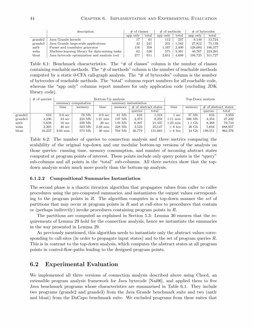
44 Chapter 6. Implementation and Experimental Evaluation
description # of classes # of methods # of bytecodesapp only total app only total app only total
grande2 Java Grande kernels 17 61 112 237 8,146 13,724grande3 Java Grande large-scale applications 42 241 231 1,162 27,812 75,139antlr Parser and translator generator 116 358 1,167 2,400 128,684 186,377weka Machine-learning library for data-mining tasks 62 530 575 3,391 40,767 223,291bloat Java bytecode optimization and analysis tool 277 611 2,651 4,699 194,725 311,727
Table 6.1: Benchmark characteristics. The “# of classes” column is the number of classescontaining reachable methods. The “# of methods” column is the number of reachable methodscomputed by a static 0-CFA call-graph analysis. The “# of bytecodes” column is the numberof bytecodes of reachable methods. The “total” columns report numbers for all reachable code,whereas the “app only” columns report numbers for only application code (excluding JDKlibrary code).
# of queries Bottom-Up analysis Top-Down analysissummary computation summary instantiation
time memory time memory # of abstract states time memory # of abstract statesqueries total queries total
grande2 616 0.6 sec 78 Mb 0.9 sec 61 Mb 616 1,318 1 sec 37 Mb 616 3,959grande3 4,236 43 sec 224 Mb 1:21 min 137 Mb 4,373 8,258 1:11 min 506 Mb 4,354 27,232antlr 5,838 16 sec 339 Mb 30 sec 149 Mb 6,207 21,437 1:23 min 1.1 Gb 8,388 79,710weka 2,205 46 sec 503 Mb 2:48 min 228 Mb 2,523 25,147 > 6 hrs 26 Gb 5,694 688,957bloat 10,237 3:03 min 573 Mb 30 min 704 Mb 36,779 131,665 > 6 hrs 24 Gb 139,551 962,376
Table 6.2: The number of queries to connection analysis and three metrics comparing thescalability of the original top-down and our modular bottom-up versions of the analysis onthose queries: running time, memory consumption, and number of incoming abstract statescomputed at program points of interest. These points include only query points in the “query”sub-columns and all points in the “total” sub-columns. All three metrics show that the top-down analysis scales much more poorly than the bottom-up analysis.
6.1.2.2 Compositional Summaries Instantiation
The second phase is a chaotic iteration algorithm that propagates values from caller to calleeprocedures using the pre-computed summaries, and instantiates the output values correspond-ing to the program points in R. The algorithm computes in a top-down manner the set ofpartitions that may occur at program points in R and at call-sites to procedures that containor (perhaps indirectly) invoke procedures containing program points in R.
The partitions are computed as explained in Section 5.3: Lemma 30 ensures that the re-quirements of Lemma 29 hold for the connection analysis, hence we instantiate the summariesin the way presented in Lemma 29.
As previously mentioned, this algorithm needs to instantiate only the abstract values corre-sponding to call-sites (in order to propagate input states) and to the set of program queries R.This is in contrast to the top-down analysis, which computes the abstract states at all programpoints in control-flow-paths leading to the designed program points.
6.2 Experimental Evaluation
We implemented all three versions of connection analysis described above using Chord, anextensible program analysis framework for Java bytecode [Nai06], and applied them to fiveJava benchmark programs whose characteristics are summarized in Table 6.1. They includetwo programs (grande2 and grande3) from the Java Grande benchmark suite and two (antlrand bloat) from the DaCapo benchmark suite. We excluded programs from these suites that

6.2. Experimental Evaluation 45
(a) Precision comparisonfor field accesses.
(b) Precision comparisonfor array accesses.
(c) Scalability comparison.
Figure 6.1: Comparison of the precision and scalability of the original top-down and our modularbottom-up versions of connection analysis. Each graph in columns (a) and (b) shows, for eachdistinct connection set size (on the X axis), the fraction of queries (on the Y axis) for whichthe analyses computed connection sets of equal or smaller size. This data is missing for thetop-down analysis in the graphs marked (*) because this analysis timed out after six hourson those benchmarks. For the remaining benchmarks, the near perfect overlap in the pointsplotted for the two analyses indicates very minor loss in precision of the bottom-up comparedwith the top-down analysis. Column (c) compares scalability of the two analyses in terms ofthe total number of abstract states computed by them. Each graph in this column shows, foreach distinct number of incoming abstract states computed at each program point (on the Xaxis), the fraction of program points (on the Y axis) with equal or smaller number of suchstates. The numbers for the top-down analysis in the graphs marked (*) were obtained at theinstant of timeout. These graphs clearly show the blow-up in the number of states computedby the top-down compared with the bottom-up analysis.

46 Chapter 6. Implementation and Experimental Evaluation
# of queries Top-Down analysistime memory # of abstract states
queries totalgrande2 616 0.9 sec 34 Mb 616 3,748grande3 4,236 51 sec 341 Mb 4,388 28,032antlr 5,838 25 sec 609 Mb 9,173 85,066weka 2,205 > 6 hrs 26 Gb 27,571 1,833,320bloat 10,237 > 6 hrs 22 Gb 389,790 2,487,372
Table 6.3: The number of queries to connection analysis and three metrics representing thescalability of the modular top-down version of the analysis on those queries: running time,memory consumption, and number of incoming abstract states computed at program points ofinterest. These points include only query points in the “query” sub-columns and all points inthe “total” sub-columns. All three metrics show that also the modular top-down analysis scalesmuch more poorly than the bottom-up analysis.
use multi-threading, since our analyses are sequential. Our larger three benchmark programsare commonly used in evaluating pointer analyses. All our experiments were performed usingOracle HotSpot JRE 1.6.0 on a Linux machine with Intel Xeon 2.13 GHz processors and 128Gb RAM.
We next compare the top-down and bottom-up approaches in terms of precision (Sec-tion 6.2.1) and scalability (Section 6.2.2). We omit the the precision results of the modifiedtop-down version of connection analysis from further evaluation as they are identical to ourbottom-up version (in principle, due to our coincidence result, as well as confirmed as a sanitycheck in our experiments).
6.2.1 Precision
We measure the precision of connection analysis by the size of the connection sets of pointervariables at program points of interest. Each such pair of variable and program point can beviewed as a separate query to the connection analysis. To obtain such queries, we chose theparallelism client proposed in the original work on connection analysis [GH96], which demandsthe connection set of each dereferenced pointer variable in the program. In Java, this corre-sponds to variables of reference type that are dereferenced to access instance fields or arrayelements. More specifically, our queries constitute the base variable in each occurrence of agetfield, putfield, aload, or astore bytecode instruction in the program. The number of suchqueries for our five benchmarks are shown in the “# of queries” column of Table 6.2. To avoidcounting the same set of queries across benchmarks, we only consider queries in applicationcode, ignoring those in JDK library code. This number of queries ranges from around 0.6K toover 10K for our benchmarks.
A precise answer to a query x.f (a field access) or x[i] (an array access) is one that is ableto disambiguate the object pointed by x from objects pointed by another variable y. In theconnection analysis abstraction, x and y are disambiguated if they are not connected. Wethereby measure the precision of connection analysis in terms of the size of the connection setof variable x, where a more precise abstraction is one where the number of other variablesconnected to x is small. To avoid gratuitously inflating this size, we perform intra-proceduralcopy propagation on the intermediate representation of the benchmarks in Chord.
Figure 6.1 provides a detailed comparison of precision based on the above metric, of the top-down and bottom-up versions of connection analysis, separately for field access queries (column(a)) and array access queries (column (b)). Each graph in columns (a) and (b) plots, for eachdistinct connection set size (on the X axis), the fraction of queries (on the Y axis) for which

6.2. Experimental Evaluation 47
each analysis computed connection sets of equal or smaller size. Graphs marked (*) indicatewhere the sizes of connection sets computed by the top-down analysis are not plotted becausethe analysis timed out after six hours. This happens for our largest two benchmarks (wekaand bloat). The graphs for the remaining three benchmarks (grande2, grande3, and antlr)show that the precision of our modular bottom-up analysis closely tracks that of the originaltop-down analysis: the points for the bottom-up and top-down analyses, denoted N and ◦,respectively, overlap almost perfectly in each of the six graphs. The ratio of the connectionset size computed by the top-down analysis to that computed by the bottom-up analysis onaverage across all queries is 0.977 for grande2, 0.977 for grande3, and 0.952 for antlr. While wedo not measure the impact of this precision loss of 2-5% on a real client, we note that for ourlargest two benchmarks, the top-down analysis does not produce any useful result.
6.2.2 Scalability
In this section we compare the scalability of the top-down and bottom-up analyses in terms ofthree different metrics: running time, memory consumption, and the total number of computedabstract states. Table 6.2 and Table 6.3 provide these data. As noted earlier (in Section 6.1.2),the bottom-up analysis runs in two phases: a summary computation phase followed by a sum-mary instantiation phase. The above data for these phases is reported in separate columns ofTable 6.2. On our largest benchmark (bloat), the bottom-up analysis takes around 50 minutesand 873 Mb memory, whereas both the top-down analyses time out after six hours, not onlyon this benchmark but also on the second largest one (weka).
The “# of abstract states” columns provide the sum of the sizes of the computed abstractionsin terms of the number of abstract states, including only incoming states at program pointsof queries (in the “queries” sub-column), and incoming states at all program points, includingthe JDK library (in the “total” sub-column). Column (c) of Figure 6.1 provides more detailedmeasurements of the latter numbers. The graphs there show, for each distinct number ofincoming states computed at each program point (on the X axis), the fraction of programpoints (on the Y axis) with equal or smaller number of incoming states. The numbers for thetop-down and the modified top-down analyses in the graphs marked (*) were obtained at theinstant of timeout. The graphs clearly show the blow-up in the number of states computed bythe top-down analyses over the bottom-up analysis.
Chapter 7
Conclusions
We show using lattice theory that when an abstract domain has enough right-modular elementsto allow transfer functions to be expressed as joins and meets with constant elements—andthe elements used in the meet are right-modular—a compositional (bottom-up) interproceduralanalysis can be as precise as a top-down analysis. Using the above, we developed a new bottom-up interprocedural algorithm for connection pointer analysis of Java programs. Our experimentsindicate that, in practice, our algorithm is nearly as precise as the existing algorithm, whilescaling significantly better. In Section A.3 we apply the same technique to derive a new bottom-up analysis for a variant of the copy-constant propagation problem [FCL09]. The algorithmutilizes a sophisticated join to compute the effect of copy statements of the form x:=y. Noticethat this is not simple under our restrictions since constant values of y are propagated into x.Indeed, we found that designing the right join operator is the key step when using our approach.
48
Bibliography
[Bod12] Eric Bodden. Inter-procedural data-flow analysis with ifds/ide and soot. In Pro-ceedings of the ACM SIGPLAN International Workshop on State of the Art in JavaProgram Analysis (SOAP’12), pages 3–8, 2012.
[BR01] Thomas Ball and Sriram Rajamani. Bebop: a path-sensitive interproceduraldataflow engine. In PASTE, pages 97–103, 2001.
[CC78] P. Cousot and R. Cousot. Static determination of dynamic properties of recursiveprocedures. In E.J. Neuhold, editor, Formal Descriptions of Programming Concepts,(IFIP WG 2.2, St. Andrews, Canada, August 1977), pages 237–277. North-Holland,1978.
[CC02] Patrick Cousot and Radhia Cousot. Modular static program analysis. In CC, pages159–178, 2002.
[CDOY11] Cristiano Calcagno, Dino Distefano, Peter W. O’Hearn, and Hongseok Yang. Com-positional shape analysis by means of bi-abduction. J. ACM, 58(6), 2011.
[CRL99] Ramkrishna Chatterjee, Barbara G. Ryder, and William Landi. Relevant contextinference. In POPL, pages 133–146, 1999.
[DDAS11] Isil Dillig, Thomas Dillig, Alex Aiken, and Mooly Sagiv. Precise and compactmodular procedure summaries for heap manipulating programs. In PLDI, pages567–5–77, 2011.
[DFS06] Julian Dolby, Stephen Fink, and Manu Sridharan. T. J. Watson Libraries for Anal-ysis. Avaliable at http://wala.sourceforge.net/, 2006.
[EGH94] M. Emami, R. Ghiya, and L. Hendren. Context-sensitive interprocedural points-toanalysis in the presence of function pointers. In PLDI, pages 242–256, 1994.
[FCL09] Charles N. Fischer, Ronald K. Cytron, and Richard J. LeBlanc. Crafting A Com-piler. Addison-Wesley Publishing Company, USA, 1st edition, 2009.
[GCRN11] Bhargav Gulavani, Supratik Chakraborty, G. Ramalingam, and Aditya Nori.Bottom-up shape analysis using lisf. ACM TOPLAS, 33(5):17, 2011.
[GH96] Rakesh Ghiya and Laurie Hendren. Connection analysis: A practical interproceduralheap analysis for C. International Journal of Parallel Programming, 24(6):547–578,1996.
[Gra78] George Gratzer. General Lattice Theory. Birkhauser Verlag, 1978.
49

50 Bibliography
[GRS05] Roberto Giacobazzi, Francesco Ranzato, and Francesca Scozzari. Making abstractdomains condensing. 6(1):33–60, 2005.
[MRV11] Ravichandhran Madhavan, Ganesan Ramalingam, and Kapil Vaswani. Purity anal-ysis: An abstract interpretation formulation. In SAS, pages 7–24, 2011.
[Nai06] Mayur Naik. Chord: A program analysis platform for Java. Available athttp://pag.gatech.edu/chord/, 2006.
[RHS95] T. Reps, S. Horwitz, and M. Sagiv. Precise interprocedural dataflow analysis viagraph reachability. In POPL, pages 49–61, 1995.
[SP81] M. Sharir and A. Pnueli. Two approaches to interprocedural data flow analysis.In S.S. Muchnick and N.D. Jones, editors, Program Flow Analysis: Theory andApplications, chapter 7, pages 189–234. Prentice-Hall, Englewood Cliffs, NJ, 1981.
[SR05] Alexandru Salcianu and Martin Rinard. Purity and side effect analysis for Javaprograms. In VMCAI, pages 199–215, 2005.
[WR99] John Whaley and Martin Rinard. Compositional pointer and escape analysis forjava programs. In OOPSLA, pages 187–206, 1999.
Appendix A
Appendix
A.1 Intraprocedural Adaptable Analysis
In this section we present a complete proof of Lemma 5 put forth in Section 4.2. We refer tothe intraprocedural abstract semantics which is shown in Table A.1.
Proof The proof is by induction on the structure of C.
• If C is a primitive command a, then,
[[a]]](d1 t d2) = ((d1 t d2) u P [[a]]]) tG[[a]]]
= ((d1 u P [[a]]]) t d2) tG[[a]]]
= ((d1 u P [[a]]]) tG[[a]]]) t d2
= [[a]]](d1) t d2
The first and last equalities hold by definition. The second equality holds because themeet element of a is right-modular and because d2 v P [[a]]]. The third equality is fromthe commutativity and associativity of t.
• If C = C1 + C2, then
[[C]]](d1 t d2) = ([[C1]]] t [[C2]]])(d1 t d2)
= [[C1]]](d1 t d2) t [[C2]]](d1 t d2)
= ([[C1]]](d1) t d2) t ([[C2]]](d1) t d2)
= ([[C1]]](d1) t [[C2]]](d1)) t d2
= [[C1 + C2]]](d1) t d2
[[a]]](d) = (d u P [[a]]]) tG[[a]]]
[[C1;C2]]](d) = [[C2]]](([[C1]]](d))[[C1 + C2]]](d) = [[C1]]](d) t [[C2]]](d)
[[C∗]]](d) = leastFix λd′. (d t ([[C]]](d)))
Table A.1: Intraprocedural Abstract Semantics for Adaptable Analysis
51
52 Appendix A. Appendix
The first equality is by the definition of [[C1 + C2]]]. The second equality is because thejoin operation is defined pointwise. The third and fourth equivalences are by the inductionassumption and the associativity and commutativity of the join operator, respectively.
• If C = C1;C2, then
[[C]]](d1 t d2) = ([[C1]]] ◦ [[C2]]])(d1 t d2)
= [[C1]]]([[C2]]](d1 t d2))
= [[C1]]]([[C2]]](d1) t d2)
= [[C1]]]([[C2]]](d1)) t d2
= [[C1;C2]]](d1) t d2
The first equivalence is by the commands composition semantics. The third and fourthequivalence are by the induction assumption.
• If C = C∗1 , then
[[C]]](d) = leastFix(F (d)) where F (d) = λd0.d t [[C1]]](d0)
We define a relation R on D.
(d, d′) ∈ R ⇔ d = d′ t d2
Claim 32 R is closed under the limit of chains.
Proof Let {xi}∞i=1, {yi}∞i=1 be two sequences, such that for all i ≥ 1, xi, yi ∈ D, and(xi, yi) ∈ R.
∀i.yi v xiTherefore,
∞⊔i=1
yi v∞⊔i=1
xi
d2 v x1 = y1 t d2 and then
d2 v∞⊔i=1
xi
thus
(
∞⊔i=1
yi) t d2 v∞⊔i=1
xi .
On the other hand,
∀i.yi v∞⊔i=1
yi
and also d2 v d2. Therefore,
∀i.xi = (yi t d2) v (∞⊔i=1
yi) t d2 ⇒∞⊔i=1
xi v (∞⊔i=1
yi) t d2 .
A.2. Triad Connection Analysis 53
Finally,∞⊔i=1
xi = (∞⊔i=1
yi) t d2
2
We prove now the claim on C.
(F (d)(⊥), F (d1)(⊥)) ∈ R
because
F (d)(⊥) = d t [[C1]]](⊥)
= d t ⊥= d1 t d2
= F (d1)(⊥) t d2
In addition to that, if (x, y) ∈ R, then (F (d)(x), F (d1)(y)) ∈ R, because
F (d)(x) = d t [[C]]](x)
= d1 t d2 t [[C1]]](y t d2)
= d1 t d2 t ([[C1]]](y) t d2)
= d1 t d2 t [[C1]]](y)
= F (d1)(y) t d2
where the third equivalence is by the assumption hypothesis. Therefore we got that
∀i > 0.(F i(d)(⊥), F i(d1)(⊥)) ∈ R
Thus, if we define xi = F i(d), yi = F i(d0) by Claim 32, we get that
(leastFix(F (d)), leastFix(F (d1))) ∈ R
i.e.[[C]]](d) = [[C]]](d1) t d2
2
A.2 Triad Connection Analysis
In this section we present the formal proofs that concern the connection analysis. In Sec-tion A.2.1 we formalize a Galois connection between the concrete domain presented in Sec-tion 3.1.2 and the abstract domain presented in Section 5.1, and we prove the soundness of theabstract semantics presented in Section 5.1.3. In Section A.2.2 we prove that the connectionanalysis is an instance of the framework presented in Section 5.2 and we prove Lemma 30 ofSection 5.3.

54 Appendix A. Appendix
A.2.1 Galois Connection
We present a Galois connection between the triad domain D of the connection analysis presentedin Section 5.1 and a standard (concrete collecting relational) domain for heap manipulatingprograms defined in Section 3.1.2.
We fix the memory states 〈sg, sl, h〉 ∈ Σ to be comprised of environments sg and sl, givingvalues to global and local variables, respectively, and a heap h. Then, we define ( · |G) andcombine as
〈sg, sl, h〉|G = 〈sg,⊥, h〉,[[combine]](〈sg, sl, h〉, 〈sg, sl, h〉, 〈s′g,⊥, h′〉)
= (〈sg, sl, h〉, 〈s′g, sl, h′〉).
Let o1 and o2 be two heap objects. We say that o1 and o2 are connected in heap h, denotedby o1 !h o2 if they are weakly connected, i.e., we can reach from one object to the other byfollowing pointers forward or backward.
We start by defining α.
α : 2Σ×Σ → Dα(∅) = ⊥α(ρ) = (
⋃(δ(σ, σ′)|〈σ, σ′〉 ∈ ρ))+ where ρ 6= ∅
where δ is defined below for σ = 〈sg, sl, h〉 and σ′ = 〈s′g, s′l, h′〉.
δ(σ, σ′) =⋂{d ∈ Equiv(Υ)|
( (sg(x) = o1 ∧ sg(y) = o2 ∧ o1 !h o2 ⇔ x′d∼= y′)
∧ (sl(x) = o1 ∧ sl(y) = o2 ∧ o1 !h o2 ⇔ xd∼= y)
∧ (sg(x) = o1 ∧ sl(y) = o2 ∧ o1 !h o2 ⇔ x′d∼= y)
∧ (sg(x) = o1 ∧ sg(y) = o2 ∧ o1 !h o2 ⇔ xd∼= y′)
∧ (sg(x) = o1 ∧ sl(y) = o2 ∧ o1 !h o2 ⇔ xd∼= y)
∧ (sg(x) = o1 ∧ sg(y) = o2 ∧ o1 !h o2 ⇔ xd∼= y))}
γ is defined as follows.
γ(⊥) = ∅γ(d) = {〈σ, σ′〉|η(d, 〈σ, σ′〉)} if d 6= ⊥
A.2. Triad Connection Analysis 55
where
η(d, 〈σ, σ′〉) = ( (sg(x) = o1 ∧ sg(y) = o2 ∧ o1 !h o2 ⇒ x′d∼= y′)
∧ (sl(x) = o1 ∧ sl(y) = o2 ∧ o1 !h o2 ⇒ xd∼= y)
∧ (sg(x) = o1 ∧ sl(y) = o2 ∧ o1 !h o2 ⇒ x′d∼= y)
∧ (sg(x) = o1 ∧ sg(y) = o2 ∧ o1 !h o2 ⇒ xd∼= y′)
∧ (sg(x) = o1 ∧ sl(y) = o2 ∧ o1 !h o2 ⇒ xd∼= y)
∧ (sg(x) = o1 ∧ sg(y) = o2 ∧ o1 !h o2 ⇒ xd∼= y))
Lemma 33 The top-down interprocedural connection analysis semantics is sound with respectto the concrete semantics.
Proof The soundness of primitive commands is trivial, thus we prove here only the soundnessof the return statement. Let dcall, dexit ∈ D. We prove that
α([[return]](γ(dexit), γ(dcall)) v [[return]]](dexit, dcall)
If dcall = ⊥ or dexit = ⊥, then
α([[return]](γ(dexit), γ(dcall)) = α(∅) = ⊥
and the claim trivially holds.Otherwise, let d = [[return]]](dexit, dcall). We show that for every 〈σ, σ′〉 ∈
[[return]](γ(dexit), γ(dcall)),δ(σ, σ′) v d .
Because d is transitively closed, this is enough in order to prove that
α([[return]](γ(dexit), γ(dcall)) = (⋃
(δ(σ, σ′)|(σ, σ′) ∈ ρ))+ v d .
Let〈σcall, σ′call〉 ∈ γ(dcall)〈σexit, σ′exit〉 ∈ γ(dexit)
such that σ′call = σexit and let
〈σ, σ′〉 = combine(σcall, σ′call, σ
′exit|G′)
Assume that aδ(σ,σ′)∼= b. We show that a
d∼= b.We prove here the case where 〈a, b〉 = 〈x, y′〉, and the proof of the other cases is very similar.
Let 〈a, b〉 = 〈x, y′〉 where x ∈ G, y′ ∈ G′. By the definition of δ, there exist o1, o2 such that
sg(x) = o1 ∧ s′g(y) = o2 ∧ o1 !h′ o2
By the definition of combine, we get that
sgcall(x) = o1 ∧ s′gexit(y) = o2 ∧ o1 !h′exito2

56 Appendix A. Appendix
Claim 34 There exist variables z, w, such that sg′call(w) = o5, sg
′call(z) = o6, o5 !h′call
o3,o6 !h′call
o4, o1 !h′exito3, and o2 !h′exit
o4.
Proof If at the entry point to the procedure, o1 and o2 are connected and y already points too2, then choosing z = y, w = y, o3 = o2, o4 = o2, o5 = o2, o6 = o2 proves the claim.
If at the entry point to the procedure, o1 and o2 are already connected but y does not pointto o2, then there exists some z such that y was assigned to it. Then there exist objects o3 ando6 such that sg
′call(z) = o6, o6 !h′call
o3 and o3 !h′exito2. Then choosing o4 = o3, o5 = o6
proves the claim.
If at the entry point to the procedure, o1 and o2 are not connected, then there must existobjects o3 and o4 such that o1 !h′exit
o3, o2 !h′exito4, which were merged into the same
connection set. Since the semantics can merge connection sets only through objects reachablefrom variables, there must exist z and w, such that sg
′call(w) = o5, sg
′call(z) = o6, o5 !h′call
o3
and o6 !h′callo4.
2
Let ˜σexit be the concrete state which is the result of changing sgexit(w) and sgexit(z) in σexit too3 and o4, respectively. By the definition of δ, δ(˜σexit, σexit) = δ(σexit, σexit). On the other hand,by the semantics definition illustrated in Section 3.1.2,
[[Cbodyp]](〈˜σexit, σexit〉) = 〈˜σexit, [[Cbodyp]](σexit)〉 = 〈˜σexit, σ′exit〉
Therefore,
〈˜σexit, σ′exit〉 ∈ γ([[Cbodyp]]](δ(˜σexit, σexit))) = γ([[Cbodyp]]
](δ(σexit, σexit))) ⊆ γ(dexit)
Finally, by the definition of α, this means that
(y′dexit∼= z) ∧ (x
dcall∼= w′) ∧ (wdexit∼= z)
and consequently
(y′d∼= x)
2
A.2.2 Connection Analysis as a Triad Analysis
In this section we prove that the requirements of Theorem 22 presented in Section 5.2.3 holdfor the connection analysis. In Section A.2.2.1 we show that the partition domain is a triaddomain, while in Section A.2.2.2 we show that the connection analysis is a triad analysis.
A.2.2.1 Triad Domain
In this section we show that the partition domain presented in Section 5.1.2 is a triad domain.
Lemma 35 D is a triad domain.

A.2. Triad Connection Analysis 57
Proof We define the projection elements
dprojin = RGdprojtmp
= RG
dprojout = RG′
dprojloc = RL
dprojinout = RG′∪Gdprojinoutloc = RG′∪G∪L
where we refer to the Ri elements illustrated in Table 5.1 of Section 5.1.
A.2.2.1.1 Modularity of the projection elements We prove now that the projectionelements are right-modular, by proving that all the element RX are right-modular.
We start by proving a few auxiliary lemmas. The first lemma gives a definition to all theelements in d t Uab. Intuitively, a relation 〈v1, v2〉 in the join result d t Uab, is either equal to〈a, b〉, or contained in d, or a consequence of the join operation, i.e., v1 and v2 are equivalentto a or b in d.
Lemma 36 Let d ∈ D, v1, v2, a, b ∈ Υ, 〈v1, v2〉 6= 〈a, b〉. Then,
(v1
dtUab∼= v2)⇒ ((v1
d∼= v2) ∨ (v1
d∼= a ∧ v2
d∼= b) ∨ (v2
d∼= a ∧ v1
d∼= b))
Proof Assume
v1
(dtUab)∼= v2
by the definition of t,
v1
(d∪Uab)+∼= v2
Then,
(v1
d∼= v2) ∨ (v1
Uab∼= v2) ∨ (v1
(d∪Uab)+\(d∪Uab)∼= v2)
Assume that v1
d6∼= v2. Since (v1, v2) 6= (a, b), by the definition of Uab, v1
Uab
6∼= v2. Therefore,
v1
(d∪Uab)+\(d∪Uab)∼= v2
and there exists a minimal alternating sequence
〈u0, v1〉〈u1, u2〉 . . . 〈un−1, un〉
such that u0 = v1, un = v2 and for all i, uid∼= ui+1, ui+1
Uab∼= ui+2 and ui 6= ui+1 ∧ ui+1 6= ui+2.
By the definition of Uab, if uiUab∼= ui+1 and ui 6= ui+1, then 〈ui, ui+1〉 = 〈a, b〉, and thus, because
of its minimality, the sequence is one of the following:
〈v1, a〉〈a, b〉〈b, v2〉 〈v1, b〉〈b, a〉〈a, v2〉 .
And from this we get that (v1
d∼= a ∧ v2
d∼= b) or (v2
d∼= a ∧ v1
d∼= b)
58 Appendix A. Appendix
2
The next lemma is a consequence of the equivalence relation. It states that the choice of anequivalence class’s representative does not matter.
Lemma 37 For all a, b ∈ Υ and d ∈ D, for all z1, z2 such that ad∼= z1, b
d∼= z2
d t Uab = d t Uz1z2
Proof Let v1
dtUab∼= v2, then, by Lemma 36, either v1
d∼= v2 or (v1
d∼= a ∧ v2
d∼= b) or (v1
d∼=
b ∧ v2
d∼= a). Assume that v1
d6∼= v2 and assume (v1
d∼= a ∧ v2
d∼= b) (the other case is symmetric).
By the transitivity of the equivalence relation (z1
d∼= v1 ∧ z2
d∼= v2), and by the definition of t,
v1
dtUz1z2∼= v2. The other direction is a consequence of the symmetry of the equivalence relation.
2
Finally, we prove a lemma that gives information regarding the structure of elements of thedomain.
Lemma 38 For every d1 ∈ D,
(d1 = ⊥) ∨ (d1 = ⊥part) ∨ (∃a, b ∈ Υ.d1 = d2 t Uab)
Notice that if d1 = Uab, d1 = ⊥part or d1 = ⊥ then d1 is join irreducible.
Proof Let d1 ∈ D. Suppose that d1 6= ⊥ and d1 6= ⊥part. Then, there exist v1
d1∼= v2, such thatv1 6= v2. Define d2 = d1 u Sv1
d2 v d1, by its definition. Also, v1
Sv1
6∼= v2, by the definition of Sv1 , and thus v1
d26∼= v2 and
d2 < d1.
Claim 39 d1 = d2 t Uv1v2
Proof We start with the left direction. Let v3
d1∼= v4 such that v3 6= v4. If v3 6= v1 ∧ v4 6= v1,
then v3
Sv1∼= v4, by the definition of Sv1 . Therefore v3
d2∼= v4 and then d2 t Uv1v2 . Otherwise,
suppose that v3 = v1 (the other case is symmetric). v4
d1∼= v2 because v3
d1∼= v4, v1
d1∼= v2 and the
assumption that v3 = v1. In addition to this, v4
Sv1∼= v2, by the definition of Sv1 . Thus v4
d2∼= v2
and v3
d2tUv2v3∼= v4. Since Uv2v3 = Uv2v1 = Uv1v2 we get
v3
d2tUv1v2∼= v4
The right direction is by the following reasoning. Assume
v3
d2tUv1v2∼= v4 .
A.2. Triad Connection Analysis 59
By Lemma 36, either v3
d2∼= v4 or (v1
d2∼= v3 ∧ v2
d2∼= v4) or (v1
d2∼= v4 ∧ v2
d2∼= v3). If v3
d2∼= v4,
then v3
d∼= v4. Otherwise, assume that (v1
d2∼= v3 ∧ v2
d2∼= v4) where d2 < d1, (the other case is
symmetric) and, since v1
d1∼= v2, by the transitivity of the relation we get that v3
d1∼= v4.
2
2
Let X ⊆ Υ. We define the separation element for the set Y as
SX = {{x} ∈ X} ∪ {Υ \X} .
We remind the reader of the definition of a separation element Sx for a variable x which wedefined in Table 4.2 of Section 4.1.1.1.
The following are claims which are consequences of the definition of the separation elementsSX and Sx.
Claim 40 For all a, b ∈ Υ, X ⊆ Υ, Uab v SX if and only if a, b /∈ X. Similarly, for alla, b, x ∈ Υ, Uab v Sx if and only if a 6= x ∧ b 6= x
Claim 41 Let v1, v2, x ∈ Υ, such that v1 6= v2. Then
(v1
d∼= v2 ∧ v1 6= x ∧ v2 6= x)⇔ v1
duSx∼= v2
Lemma 42 For any X ⊆ Υ, RX is a right-modular element.
Proof We need to prove that for every d1, d2 ∈ D such that d2 v RX it holds that
(d1 uRX) t d2 = (d1 t d2) uRX
We will prove that any element SX is right-modular. Since PX = SΥ\X , this is enough to provethe lemma.
The proof goes by induction on d2’s structure, where we use Lemma 38, to make theassumptions on its structure.
Base case If d2 = ⊥part or d2 = ⊥, then the claim trivially holds.
Otherwise, assume d2 = Uab. We need to prove that for every d1 ∈ D, and SX w Uab
(d1 u SX) t Uab = (d1 t Uab) u SX
Again, the proof is by induction, this time on |X|. The base case is given by the followinglemma.
Lemma 43 For each element d ∈ D, a, b, x ∈ Υ, if a 6= x ∧ b 6= x.
(d t Uab) u Sx = (d u Sx) t Uab

60 Appendix A. Appendix
Proof 1. Assume
v1
(dtUab)uSx∼= v2
and v1 6= v2. By Claim 41,
v1
dtUab∼= v2
and v1 6= x and v2 6= x. Also by Lemma 36, v1
d∼= v2 or (v1
d∼= a∧v2
d∼= b) or (v1
d∼= b∧v2
d∼= a).
If v1
d∼= v2, then v1
duSx∼= v2 because v1 6= x and v2 6= x (Claim 41) and obviously
v1
(duSx)tUab∼= v2 .
Otherwise, assume (v1
d∼= a ∧ v2
d∼= b), (the other case is symmetric). Again (Claim 41),
since v1 6= x ∧ v2 6= x ∧ a 6= x ∧ b 6= x, (v1
duSx∼= a ∧ v2
duSx∼= b) and by the definition of t,
v1
(duSx)tUab∼= v2 .
2. Assume
v1
(duSx)tUab∼= v2 .
Again, we use Lemma 36. If v1
duSx∼= v2, then v1
d∼= v2 and v 6= x, v2 6= x (Claim 41). Then
v1
dtUab∼= v2 and by Claim 41,
v1
(dtUab)uSx∼= v2
Otherwise, assume (the other case is symmetric) (v1
duSx∼= a ∧ v2
duSx∼= b). By Claim 41
(v1
d∼= a ∧ v2
d∼= b) ∧ v1 6= x ∧ v2 6= x ∧ a 6= x ∧ b 6= x. Then v1
dtUab∼= v2 and by Claim 41,
v1
(dtUab)uSx∼= v2
2
We prove now the inductive step.
(d t Uab) u SX = (d t Uab) u (ux∈XSx) By the definition of SX
= (d t Uab) u (ux∈X\{x′}Sx u Sx′)= (d t Uab) u (ux∈X\{x′}Sx) u Sx′ By the associativity of meet operator
= ((d t Uab) u SX\{x′}) u Sx′ By the definition of SX
= ((d u SX\{x′}) t Uab) u Sx′ By the induction hypothesis

A.2. Triad Connection Analysis 61
Define d2 = d u SX\{x′}. Then we get
= (d2 t Uab) u Sx′= (d2 u Sx′) t Uab By Lemma 43
= ((d u SX\{x′}) u Sx′) t Uab By the definition of d2
= (d u (SX\{x′} u Sx′)) t Uab By the associativity of the meet operator
= (d u SX) t Uab
Inductive Step Let Uab 6= d2 ∈ D. By Lemma 38, d2 = d′2 t Uab, such that d′2 < d2. Thenwe get
SX u (d1 t d2) = SX u (d1 t (d′2 t Uab))= SX u ((d1 t Uab) t d′2) By the associativity and commutativity of the join operator
= (SX u (d1 t Uab)) t d′2 By the induction hypothesis
= ((SX u d1) t Uab) t d′2 By the induction hypothesis
= (SX u d1) t (Uab t d′2) By the associativity of join
= (SX u d1) t d2
2
A.2.2.1.2 Isomorphism functions We define the isomorphism functions
fcall = λd.d[g ↔ g′]
fexit = λd.d[g ↔ g]
finout = λd.d[g ↔ g′]
where d[g ↔ g] replaces all occurrences g with g and vice versa.
Claim 44fcall(RG′) = RG, fcall(RG) = RG, fcall(RG) = RG′
fexit(RG′) = RG′ , fexit(RG) = RG, fexit(RG) = RGfinout(RG′) = RG, finout(RG) = RG′ , finout(RG) = RG
Proof We prove the claim on fcall and RG′ , the other cases being symmetric.
fcall(RG′) = fcall({G′} ∪ {{x}|x ∈ Υ \ G′})= {G} ∪ {{x}|x ∈ Υ \ G} = RG
2
Claim 45 For all d ∈ Dout
fexit(finout(d)) = fcall(d)
Proof By the definition of fexit, for all d ∈ Dout, if afexit(d)∼= b and a 6= b, then 〈a, b〉 = 〈x, y〉 for
some x, y ∈ G. Moreover, the same is true for all 〈a, b〉 ∈ fcall(d).
(xfexit(finout(d))∼= y)⇔ (x
finout(d)∼= y)⇔ (x′d∼= y′)

62 Appendix A. Appendix
On the other hand,
(xfcall(d)∼= y)⇔ (x′
d∼= y′)
2
Claim 46 For all d ∈ Din
fcall(d) = d
Proof fcall renames ′ to , thus for every x, y ∈ G
(xd∼= y)⇔ (x
fcall(d)∼= y)
and since for every x /∈ G, x is a singleton in every d ∈ Din, we get that for every x, y /∈ G, x 6= y
(xd∼= y)⇔ (x
fcall(d)∼= y)
2
Finally, the ιentry requirement is by the definition of ιentry in the partition domain.
2
A.2.2.2 Triad Analysis
In this section, we show that the connection analysis presented in Section 5.1.3 is a triadanalysis.
Lemma 47 The connection analysis is a triad analysis.
Proof The partition domain is a triad-domain. Moreover, we show in the previous section thatall the RX elements are right-modular, and since for any primitive command a
P [[a]]] = RX\{x′}
for some x′ ∈ G′, we get that all the atomic commands are conditionally adaptable.
Finally, for every d ∈ Din,
d = {{a1, . . . , ak}} ∪ {{x}|x ∈ Υ \ G} where ai ⊆ G, 1 ≤ i ≤ k
and thusd v {Υ \ {x}} ∪ {{x′}} where x′ ∈ G′
2
Lemma 48 For all C,
[[C]]](ιentry) = (fcall(ιentry) t fexit([[C]]](ιentry)))|inoutloc .
Proof Let dC = [[C]]](ιentry) and dS = (fcall(ιentry) t fexit([[C]]](ιentry)))|inoutloc. We show theresult by proving that dC v dS and that dS v dC .
A.3. Triad Copy Constant Propagation Analysis 63
Let a, b ∈ Υ such that adC∼= b. We prove the case where 〈a, b〉 = 〈x, y〉, as the other cases
are similar to it. By the definition of ιentry and of fcall, xfcall(ιentry)∼= x and y
fcall(ιentry)∼= y.
xfexit(dC)∼= y ⇒ x
fcall(ιentry)tfexit(dC)∼= y ⇒ xdS∼= y .
Let a, b ∈ Υ such that adC∼= b and assume that 〈a, b〉 = 〈x, y〉. x
(fexit([[C]]](ιentry))∪fcall(ιentry))+∼=
y and since x, y ∈ G, then x(fexit([[C]]](ιentry))∪fcall(ιentry))+\(fexit([[C]]](ιentry))∪fcall(ιentry))∼= y. Then,
xfexit([[C]]](ιentry))∼= y and therefore
xdC∼= y .
2
A.3 Triad Copy Constant Propagation Analysis
In this section we describe an encoding of a bottom-up interprocedural copy constant propaga-tion analysis as a triad analysis.
A.3.1 Programming Language
We define a simple programming language which manipulates integer variables. The languageis defined according to the requirements of our general framework. (See Chapter 3.) In thissection, we assume that programs have only global integer variables g ∈ G which are initializedto 0. We also assume that the primitive commands a ∈ PComm are of the form
x := c , x := y , and x := * ,
pertaining to assignments to a variable x of a constant value c, of the value of a variable y, orof an unknown value, respectively. We denote by KP ⊂fin N the finite set of constants whichappear in a program P . We assume KP contains 0. We denote by GP ⊂fin G the finite set ofglobal variables which appear in a program P .
In the following, we assume a fixed arbitrary program P and denote by K = KP the (fixedfinite) set of constants that appear in P , and by G = GP the (fixed finite) set of global variablesof P .
For technical reasons, explained in Section A.3.5, we assume that the analyzed programcontains a special global variable t which is not used directly by the program, but is used onlyto implement copy assignments of the form x := y using the following sequence of assignments
t:=y; y:=0; x:=0; y:=t; x:=t; t:=0.
(Note that, in particular, we assume that there are no statements of the form x := x.)

64 Appendix A. Appendix
A.3.2 Concrete Semantics
A.3.2.1 Standard Intraprocedural Concrete Semantics
A standard memory state s ∈ S = G 7→ N maps variables to their integer values. The meaningof primitive commands a ∈ AComm is standard, and defined below.
[[x := c]](s) = {(s[x 7→ [[c]]])}[[x := y]](s) = {(s[x 7→ s(y)])}[[x := ∗]](s) = {(s[x 7→ n]) | n ∈ N}
Note that [[a]] : S → 2S for a primitive a.
A.3.2.2 Relational Concrete Semantics
An input-output pair of standard memory states r = (s, s′) ∈ R = S × S records the valuesof variables at the entry to the procedure (s) and at the current state (s′). The meaningof intraprocedural statements is lifted to input-output pairs as described in Chapter 3. Theinterprocedural semantics is defined, as described in Chapter 3, using the functions ·|G : S → Sand [[combine]] : S × S × S → R, whose meaning is defined below:
s|G = s[[combine]](s1, s2, s3) = (s1, s3)
Informally, the projection of the state on its global part does not modify the state due to ourassumption that a state is a mapping of global variables to values. For a similar reason, thecombination of the caller’s input-output pair at the call-site with that of the callee at the exit-site results in a pair of memory states where the first one records the memory at the entry-siteof the caller and the second one records the state at the exit-site of the callee.
A.3.3 Abstract Semantics
Notations. For every global variable g ∈ G, g denotes the value of g at the entry to aprocedure and g′ denotes its current value. Similarly to the connection analysis, we use anadditional set G of variables to compute the effect of procedure calls. We denote by
υ ∈ Υ = G′ ∪G ∪ G
the set of all annotated variables which are ranged by a meta variable υ.
We denote byζ ∈ VAL = Υ ∪K ∪ {∗}
the set of abstract values ranged over by ζ. VAL is comprised of annotated variables,constants which appear in the program, and the special value ∗.
A.3.3.1 Abstract Domain
Let Dmap be the set of all maps from variables υ ∈ Υ to 2VAL
Dmap = Υ 7→ 2VAL .
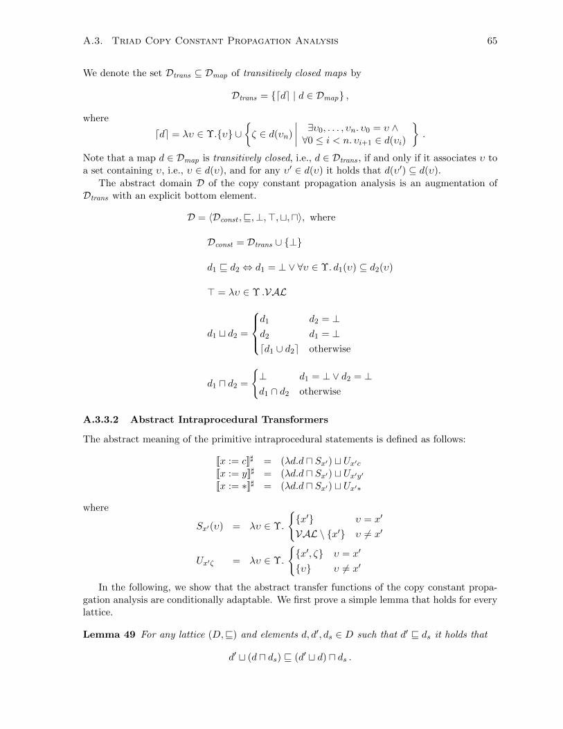
A.3. Triad Copy Constant Propagation Analysis 65
We denote the set Dtrans ⊆ Dmap of transitively closed maps by
Dtrans = {dde | d ∈ Dmap} ,
where
dde = λυ ∈ Υ.{υ} ∪{ζ ∈ d(υn)
∣∣∣∣ ∃υ0, . . . , υn. υ0 = υ ∧∀0 ≤ i < n. υi+1 ∈ d(υi)
}.
Note that a map d ∈ Dmap is transitively closed, i.e., d ∈ Dtrans , if and only if it associates υ toa set containing υ, i.e., υ ∈ d(υ), and for any υ′ ∈ d(υ) it holds that d(υ′) ⊆ d(υ).
The abstract domain D of the copy constant propagation analysis is an augmentation ofDtrans with an explicit bottom element.
D = 〈Dconst ,v,⊥,>,t,u〉, where
Dconst = Dtrans ∪ {⊥}
d1 v d2 ⇔ d1 = ⊥ ∨ ∀υ ∈ Υ. d1(υ) ⊆ d2(υ)
> = λυ ∈ Υ .VAL
d1 t d2 =
d1 d2 = ⊥d2 d1 = ⊥dd1 ∪ d2e otherwise
d1 u d2 =
{⊥ d1 = ⊥ ∨ d2 = ⊥d1 ∩ d2 otherwise
A.3.3.2 Abstract Intraprocedural Transformers
The abstract meaning of the primitive intraprocedural statements is defined as follows:
[[x := c]]] = (λd.d u Sx′) t Ux′c[[x := y]]] = (λd.d u Sx′) t Ux′y′[[x := ∗]]] = (λd.d u Sx′) t Ux′∗
where
Sx′(υ) = λυ ∈ Υ.
{{x′} υ = x′
VAL \ {x′} υ 6= x′
Ux′ζ = λυ ∈ Υ.
{{x′, ζ} υ = x′
{υ} υ 6= x′
In the following, we show that the abstract transfer functions of the copy constant propa-gation analysis are conditionally adaptable. We first prove a simple lemma that holds for everylattice.
Lemma 49 For any lattice (D,v) and elements d, d′, ds ∈ D such that d′ v ds it holds that
d′ t (d u ds) v (d′ t d) u ds .
66 Appendix A. Appendix
Proof By the definition of t it holds that
d v (d′ t d) and d′ v (d′ t d) .
By the monotonicity of u, we get that
d u ds v (d′ t d) u ds and d′ u ds v (d′ t d) u ds .
By the monotonicity and the idempotence of t, we get that
(d′ u ds) t (d u ds) v (d′ t d) u ds .
By the assumption, d′ v ds. Hence, d′ u ds = d′, and it follows that
d′ t (d u ds) v (d′ t d) u ds .
2
Definition 50 (General projection and separation elements) Let X ⊆ Υ. We denoteby
SX(υ) = λυ ∈ Υ.
{{υ} υ ∈ XVAL \X υ 6∈ X
the separation element of X and byRX = SΥ\X
the projection element of X.
Lemma 51 For every X ⊆ Υ, SX is right-modular.
Proof We need to prove that for all d, d′ ∈ D such that d′ v SX it holds that
(d′ t d) u SX = d′ t (d u SX) .
By Lemma 49, it holds that
(d′ t d) u SX w d′ t (d u SX) .
Thus it suffices to show that
d1 = (d′ t d) u SX v d′ t (d u SX) = d2 . (∗)
We prove (*) by induction on the size of X.
Base Case. For |X| = 1, we get that SX = S{υ} for some υ ∈ Υ. Pick υ0 ∈ Υ. We need toshow that d1(υ0) ⊆ d2(υ0). There can be two case: either υ0 = υ or not.
If υ0 = υ, then d1(υ0) ⊆ S{υ}(υ0) = {υ0}. By definition of the domain, which includes onlytransitively closed maps, υ0 ∈ d′(υ0). Hence, d1(υ0) ⊆ {υ0} ⊆ d2(υ0).
Otherwise, υ0 6= υ. Pick υ1 ∈ d1(υ0). By the definition of S{υ} and the meet operation,υ1 6= υ, and again by the definition of the meet operation, υ1 ∈ (d′td)(υ0). Thus, there exists aminimal sequence ζ0, . . . , ζn such that ζ0 = υ0∧ζn = υ1 and for all 0 ≤ i < n, ζi+1 ∈ d′(ζi)∪d(ζi).

A.3. Triad Copy Constant Propagation Analysis 67
Claim 52 For all 0 ≤ j < n, ζj 6= υ.
Proof ζ0 = υ0 6= υ, by the assumption.
Assume that there exists some 0 < j < n such that ζj = υ. By the minimality of thesequence, ζj−1 6= υ and ζj+1 6= υ, and since d′ v S{υ}, ζj = υ /∈ d′(ζj−1) and ζj+1 /∈ d′(ζj) =d′(υ) and thus ζj ∈ d(ζj−1) and ζj+1 ∈ d(ζj). d is transitively closed and from this, ζj+1 ∈d(ζj−1). Thus, the sequence ζ0, . . . , ζj−1, ζj+1, . . . , ζn is a valid sequence for υ0, υ1, and this is acontradiction to the minimality of the original sequence.
2
By the claim, we got that for all 0 ≤ j < n,
ζj+1 ∈ (d′(ζj) ∪ d(ζj)) \ {υ}⇒ ζj+1 ∈ (d′(ζj) ∪ d(ζj)) ∩ S{υ}(ζj) By the definition of S{υ}
= (d′(ζj) ∩ S{υ}(ζj)) ∪ (d(ζj) ∩ S{υ}(ζj))= d′(ζj) ∪ (d(ζj) ∩ S{υ}(ζj)) By d′(ζj) ⊆ S{υ}(ζj)= d′(ζj) ∪ (d u S{υ})(ζj) .
Therefore we can create a sequence for υ0, υ1, by taking elements only from d′ ∪ (duS{υ}), andhence υ1 ∈ (d′ t (d u S{υ}))(υ0).
Induction Step. Assume that the induction assumption holds for sets X such that |X| = n,we will prove the claim for sets X such that |X| = n+ 1. Let υ ∈ X be an arbitrary element.Notice that by its definition
SX = SX\{υ} u S{υ} .
Therefore,(d′ t d) u SX = (d′ t d) u (SX\{υ} u S{υ})
= ((d′ t d) u SX\{υ}) u S{υ}v (d′ t (d u SX\{υ})) u S{υ}= d′ t ((d u SX\{υ}) u S{υ})= d′ t (d u (SX\{υ} u S{υ}))= d′ t (d u SX)
2
Lemma 53 The abstract transfer functions of the atomic commands are conditionally adapt-able.
Proof By Lemma 51, Sx′ = S{x′} is right-modular and all the transfer functions are of form
f = λd.((d u dp) t dg) .
where dp = Sx′ for some x′ ∈ Υ.
2

68 Appendix A. Appendix
A.3.4 Soundness of the Top Down Analysis
The soundness of the copy constant propagation analysis is formalized by the concretizationfunction γ : D → 2S×S , where
(s, s′) ∈ γ(d) ⇐⇒(∀x ∈ G. (s(x) ∈ d(x) ∩K) ∨ (∗ ∈ d(x))
)∧(∀x′ ∈ G′. s′(x) ∈ ((d(x) ∩K) ∪ {s(y) | y ∈ d(x))}) ∨ (∗ ∈ d(x))
).
Intuitively, an input-output pair (s, s′) is conservatively represented by an abstract element d ifand only if (a) the input state maps a variable g to n if n is one of the constants mapped to gby d or if ∗ ∈ d(g) and (b) the output state maps a variable g to n if n is one of the constantsmapped to g′ by d, the value of global variable y at the entry state that is mapped to g′ by d,or if ∗ ∈ d(g′).
Lemma 54 (Soundness) The abstract transformers pertaining to intraprocedural primitivecommands, |G, and combine over-approximate the concrete ones.
A.3.5 Precision Improving Transformations
In Section A.3.1, we place certain restrictions on the analyzed programs. Specifically, we forbidcopy assignments of the form x:=y between arbitrary global variables x and y, and, instead,require that the value of y be copied to x through a sequence of assignments that use a temporaryvariable t. In the concrete semantics, our requirements do not affect the values of the program’svariables outside of the sequences of intermediate assignments. In the abstract semantics,however, adhering to our requirements can improve the precision of the analysis, as we explainbelow.
Consider the execution of the sequence of abstract transformers pertaining to the (nondeterministic) command x:=y + y:=3 on an abstract state d, in which 3 6∈ d(y′). Applyingthe abstract transformer [[x := y]]] to d results in an abstract element d′, where y′ ∈ d(x′).Applying [[y := 3]]] to d results in an abstract state d′′, where 3 ∈ d′′(y′). Perhaps surprisingly,in the abstract state d′′′ = d′ t d′′, which conservatively represent the possible states afterthe non-deterministic choice (+), we get that 3 ∈ d′′′(x′). This is sound, but imprecise. Thereason for the imprecision is that our domain includes only transitively closed maps and havingy′ ∈ d′(x′) results in an undesired correlation between the possible values of x in d′′′ and that ofy in d′′. In particular, the assignment of 3 to y is propagated to x in a flow-insensitive manner.
Rewriting the copy assignment using t according to our restrictions breaks such undesiredcorrelations. Consider, for example, the sequence of abstract transformers pertaining to thepreviously mentioned command: t:=y; y:=0; x:=0; y:=t; x:=t; t:=0, and apply this se-quence to d. In the abstract state d arising just before t is assigned 0 we get that t′ ∈ d(x′)and t′ ∈ d(y′) but y′ 6∈ d(x′) and x′ 6∈ d(y′). Assigning 0 to t breaks the correlation between t
and x and y.
A.3.6 Copy Constant Propagation as a Triad Analysis
A.3.6.1 Triad Domain
Lemma 55 D is a triad domain.

A.3. Triad Copy Constant Propagation Analysis 69
Projection Elements
Proof We define the projection elements
dprojin = RG
dprojtmp= RG
dprojout = RG′
By Lemma 51, dprojin , dprojtmpand dprojout are right-modular.
Isomorphism functions We define the renaming functions
fΥcall, f
Υexit, f
Υinout : Υ→ Υ
fΥcall(υ) =
υ υ = υ′
υ′ υ = υ
υ otherwise
fΥexit(υ) =
υ υ = υ
υ υ = υ
υ otherwise
fΥinout(υ) =
υ υ = υ′
υ′ υ = υ
υ otherwise
Let fVALcall , fVALexit , fVALinout be the renaming function induced on 2VAL and finally let fcall, fexit,finout be the renaming functions induced on D,
fi(d) =
{⊥ d = ⊥λυ ∈ Υ. fVALi (d(fΥ
i−1
(υ))) otherwise(A.1)
where i ∈ [call, inout, exit].
Claim 56fcall(RG′) = RG, fcall(RG) = RG, fcall(RG) = RG′
fexit(RG′) = RG′ , fexit(RG) = RG, fexit(RG) = RGfinout(RG′) = RG, finout(RG) = RG′ , finout(RG) = RG
Proof We prove the claim on fcall and RG′ . The other cases are symmetric.
fcall(RG′) = fcall
(λυ ∈ Υ.
{{υ} υ ∈ Υ \ G′
K ∪ G′ υ ∈ G′
)
= λυ ∈ Υ.
{{υ} υ ∈ Υ \ GK ∪ G υ ∈ G
= RG
2

70 Appendix A. Appendix
Claim 57 For all d ∈ Dout
fexit(finout(d)) = fcall(d)
Proof Let d ∈ Dout and let υ ∈ Υ. If d = ⊥ then
fcall(d) = fexit(finout(d)) = ⊥ .
Otherwise, by Eq.A.1,
fcall(d)(υ) = fVALcall (d(fΥcall−1
(υ)))
and
((fexit ◦ finout)(d))(υ) = fexit(finout(d))(υ)
= fVALexit (finout(d)(fΥexit−1
(υ))
= fVALexit (fVALinout (d(fΥinout
−1(fΥ
exit−1
(υ))
= (fVALexit ◦ fVALinout )(d(fΥinout
−1 ◦ fΥexit−1
)(υ))
If υ /∈ G, then
fΥcall−1
(υ) /∈ G′
andfΥinout
−1 ◦ fΥexit−1
(υ) /∈ G′
and therefored(fΥ
call−1
(υ)) = {fΥcall−1
(υ)}
andd(fΥ
inout−1 ◦ fΥ
exit−1
(υ)) = {fΥinout
−1 ◦ fΥexit−1
(υ)}
Hence,
fcall(d)(υ) = fVALcall ({fΥcall−1
(υ)}) = {υ}
and(fexit ◦ finout)(d)(υ) = (fVALexit ◦ fVALinout )({fΥ
inout−1 ◦ fΥ
exit−1
(υ)}) = {υ}
Otherwise, if υ ∈ G, by the definition of the renaming functions
fΥcall−1
(υ) = (fΥinout
−1 ◦ fΥexit−1
)(υ)
and by the definition of Dout,
d(fΥcall−1
(υ)) ⊆ G′
and therefore again by the definition of the renaming functions
fVALcall (d(fΥcall−1
(υ))) = (fVALexit ◦ fVALinout )(d(fΥcall−1
(υ)))
2
Claim 58 For all d ∈ Din
fcall(d) = d
Proof By the definition of Din and of fcall.
2

A.3. Triad Copy Constant Propagation Analysis 71
ιentry element We define
ιentry = [υ′ 7→ {υ′, υ} | υ ∈ G] ∪ [υ 7→ {υ′, υ} | υ ∈ G] ∪ [υ 7→ {υ} | υ ∈ G]
Claim 59 For every d ∈ Dout, d t ιentry = finout(d) t ιentry.
Proofd t ιentry = dd ∪ ιentrye
=
λυ ∈ Υ.
d(g′) ∪ {g′, g} υ = g′ ∈ G′
{g} ∪ {g′, g} υ = g ∈ G
{g} ∪ {g} υ = g ∈ G
= λυ ∈ Υ.
{{h, h′ | h′ ∈ d(g′)} υ = g′ ∈ G′ ∨ υ = g ∈ G
{g} υ = g ∈ G
=
λυ ∈ Υ.
{g′} ∪ {g′, g} υ = g′ ∈ G′
{h | h′ ∈ d(g′)} ∪ {g′, g} υ = g ∈ G
{g} ∪ {g} υ = g ∈ G
=
λυ ∈ Υ.
{g′} ∪ {g′, g} υ = g′ ∈ G′
finout(d)(g) ∪ {g′, g} υ = g ∈ G
{g} ∪ {g} υ = g ∈ G
= finout(d) t ιentry
2
2