Modular Forms of One Variable Don Zagier - Max Planck...
63
Modular Forms of One Variable Don Zagier Notes based on a course given in Utrecht, Spring 1991 1
Transcript of Modular Forms of One Variable Don Zagier - Max Planck...
Modular Forms of One Variable
Don Zagier
Notes based on a course given in Utrecht, Spring 1991
1

Table of Contents
Chapter 0. The notion of modular forms and a survey of the main examples 1
Exercises 7
Chapter 1. Modular forms on SL2(Z) 8
1.1 Eisenstein series 8
1.2 The discriminant function 10
1.3 Modular forms and differential operators 12
Exercises 14
Chapter 2. Hecke theory 15
2.1 Hecke operators 15
2.2 Eigenforms 17
2.3 L-series 20
2.4 Modular forms of higher level 23
Exercises 26
Chapter 3. Theta functions 27
3.1 Theta series of definite quadratic forms 27
3.2 Theta series with spherical coefficients 30
Exercises 31
Chapter 4. The Rankin-Selberg method 32
4.1 Non-holomorphic Eisenstein series 32
4.2 The Rankin-Selberg method (non-holomorphic case) and applications 34
4.3 The Rankin-Selberg method (holomorphic case) 37
Exercises 39
Chapter 5. Periods of modular forms 40
5.1 Period polynomials and the Eichler-Shimura isomorphism 40
5.2 Hecke operators and algebraicity results 43
Exercises 45
Chapter 6. The Eichler-Selberg trace formula 47
6.1 Eisenstein series of half-integral weight 47
6.2 Holomorphic projection 49
6.3 The Eichler-Selberg trace formula 50
Exercises 53
Appendices
A1. The Poisson summation formula 54
A2. The gamma function and the Mellin transform 55
A3. Dirichlet characters 57
Exercises 58
0
Chapter 0. The Notion of Modular Forms
and a Survey of the Main Examples
The word “modular” refers to the moduli space of complex curves (= Riemann surfaces)
of genus 1. Such a curve can be represented as C/Λ where Λ ⊂ C is a lattice, two lattices Λ1
and Λ2 giving rise to the same curve if Λ2 = λΛ1 for some non-zero complex number λ. A
modular function assigns to each lattice Λ a complex number F (Λ) with F (Λ1) = F (Λ2)
if Λ2 = λΛ1. Since any lattice Λ = Zω1 +Zω2 is equivalent to a lattice of the form Zτ +Z
with τ (= ω1/ω2) a non-real complex number, the function F is completely specified by the
values f(τ) = F (Zτ+Z) with τ in C\R or even, since f(τ) = f(−τ), with τ in the complex
upper half-plane H = { τ ∈ C | ℑ(τ) > 0}. The fact that the lattice Λ is not changed by
replacing the basis {ω1, ω2} by the new basis aω1 + bω2, cω1 + dω2 (a, b, c, d ∈ Z, ad− bc =
±1) translates into the modular invariance property f(aτ + b
cτ + d) = f(τ). Requiring that
τ always belong to H is equivalent to looking only at bases {ω1, ω2} which are oriented
(i.e. ℑ(ω1/ω2) > 0) and forces us to look only at matrices(acbd
)with ad − bc = +1; the
group SL2(Z) of such matrices will be denoted Γ1 and called the (full) modular group.
Thus a modular function can be thought of as a complex-valued function on H which is
invariant under the action τ 7→ (aτ + b)/(cτ +d) of Γ1 on H. Usually we are interested only
in functions which are also holomorphic on H (and satisfy a suitable growth condition at
infinity) and will reserve the term “modular function” for these. The prototypical example
is the modular invariant j(τ) = e−2πiτ + 744 + 196884e2πiτ + · · · (cf. 1.2).
However, it turns out that for many purposes the condition of modular invariance is
too restrictive. Instead, one must consider functions on lattices which satisfy the identity
F (Λ1) = λkF (Λ2) when Λ2 = λΛ1 for some integer k, called the weight. Again the
function F is completely determined by its restriction f(τ) to lattices of the form Zτ + Z
with τ in H, but now f must satisfy the modular transformation property
(1) f(aτ + b
cτ + d
)= (cτ + d)kf(τ)
rather than the modular invariance property required before. The advantage of allowing
this more general transformation property is that now there are functions satisfying it
which are not only holomorphic in H, but also “holomorphic at infinity” in the sense that
their absolute value is majorized by a polynomial in max{1,ℑ(τ)−1}. This cannot happenfor non-constant Γ1-invariant functions by Liouville’s theorem (the function j(τ) above, for
instance, grows exponentially as ℑ(τ) tends to infinity). Holomorphic functions f : H → C
satisfying (1) and the growth condition just given are called modular forms of weight
k, and the set of all such functions—clearly a vector space over C—is denoted by Mk or
Mk(Γ1). The subspace of functions whose absolute value is majorized by a multiple of
ℑ(τ)−k/2 is denoted by Sk or Sk(Γ1), the space of cusp forms of weight k. One also looks
at the spaces Mk(Γ) and Sk(Γ), defined as above but with (1) only required to hold for1
(acbd
)∈ Γ, for subgroups Γ ⊂ Γ1 of finite index, e.g. the subgroup Γ0(N) consisting of all(
acbd
)∈ Γ1 with c divisible by a fixed integer N .
The definition of modular forms which we have just given may not at first look very
natural. The importance of modular forms stems from the conjunction of the following two
facts:
(i) They arise naturally in a wide variety of contexts in mathematics and physics and
often encode the arithmetically interesting information about a problem.
(ii) The space Mk is finite-dimensional for each k.
The point is that if dimMk = d and we have more than d situations giving rise to modular
forms inMk, then we automatically have a linear relation among these functions and hence
get “for free” information—often highly non-trivial—relating these different situations. The
way the information is “encoded” in the modular forms is via the Fourier coefficients. From
the property (1) applied to the matrix(acbd
)=
(1011
)we find that any modular form f(τ) is
invariant under τ 7→ τ + 1 and hence, since it is also holomorphic, has a Fourier expansion
as∑ane
2πinτ . The growth conditions definingMk and Sk as given above are equivalent to
the requirement that an vanish for n < 0 or n ≤ 0, respectively (this is the form in which
these growth conditions are usually stated). What we meant by (i) above is that nature—
both physical and mathematical—often produces situations described by numbers which
turn out to be the Fourier coefficients of a modular form. These can be as disparate as
multiplicities of energy levels, numbers of vectors in a lattice of given length, sums over the
divisors of integers, special values of zeta functions, or numbers of solutions of Diophantine
equations. But the fact that all of these different objects land in the little spaces Mk forces
the existence of relations among their coefficients. To give the flavour of the kind of results
one can obtain, we will now list some of the known constructions of modular forms and
some of the number-theoretic identities one obtains by studying the relations among them.
More details and many more examples will be given in the following chapters.
Eisenstein series. For each integer k ≥ 2, we have a function Gk(τ) with the Fourier
development
Gk(τ) = ck +∞∑
n=1
σk−1(n) e2πinτ ,
where σk−1(n) for n > 0 denotes the sum of the (k − 1)st powers of the (positive) divisors
of n and ck is a certain rational number, e.g.,
G2(τ) = − 1
24+ q + 3q2 + 4q3 + 7q4 + 6q5 + 12q6 + 8q7 + 15q8 + · · ·
G4(τ) =1
240+ q + 9q2 + 28q3 + 73q4 + 126q5 + 252q6 + · · ·
G6(τ) = − 1
504+ q + 33q2 + 244q3 + 1057q4 + · · ·
G8(τ) =1
480+ q + 129q2 + 2188q3 + · · ·
2

(here and from now on we use q to denote e2πiτ ). We will study these functions in Chapter
1 and show that Gk for k > 2 is a modular form of weight k, while G2 is “nearly” a modular
form of weight 2 (for instance, G2(τ)−NG2(Nτ) is a modular form of weight 2 on Γ0(N)
for all N). This will immediately have arithmetic consequences of interest. For instance,
because the space of modular forms of weight 8 is one-dimensional, the forms 120G4(τ)2
and G8(τ), which both have weight 8 and constant term 1/480, must coincide, leading to
the far from obvious identity
(2) σ7(n) = σ3(n) + 120n−1∑
m=1
σ3(m)σ3(n−m) (n > 0),
the first example of the above-mentioned phenomenon that the mere existence of modular
forms, coupled with the finite-dimensionality of the spaces in which they lie, gives instant
proofs of non-trivial number-theoretical relations. Another number-theoretical application
of the Gk is connected with the constant terms ck, which turn out to be essentially equal
to the values of the Riemann zeta-function ζ(s) =∞∑
n=1
1
nsat s = k, so that one obtains a
new proof of and new insight into the identities
ζ(2) =π2
6, ζ(4) =
π4
90, ζ(6) =
π6
945. . .
proved by Euler.
The discriminant function. This is the function defined by the infinite product
∆(τ) = q
∞∏
n=1
(1− qn)24 = q − 24q2 + 252q3 − 1472q4 + 4830q5 − 6048q6 + · · · .
We will show in Chapter 1 that it is a cusp form of weight 12. This at once leads to
identities like 1728∆ = (240G4)3 − (504G6)
2 which let us express the coefficients of ∆ in
terms of the elementary number-theoretic functions σk−1(n). More important, it provides
the first example of one of the most interesting and important properties of modular forms.
Namely, the coefficients of ∆ are multiplicative, e.g., the coefficient −6048 of q6 in the above
expansion is the product of the coefficients −24 and 252 of q2 and q3 (more generally, the
coefficient of qmn is the product of the coefficients of qm and qn whenever m and n are
coprime). This property, which was observed by Ramanujan in 1916 and proved by Mordell
the following year, was developed by Hecke into the theory of Hecke operators, which is at
the center of the whole theory of modular forms and will be discussed in detail in Chapter
2.
Theta series. Consider the Jacobi theta function
θ(τ) =∑
m∈Z
qm2
= 1 + 2q + 2q4 + 2q9 + · · · .
3

The powers of θ(τ) tell us the number of ways of representing an integer as a sum of a
given number of squares, e.g.,
θ(τ)4 =∑
m1,m2,m3,m4
qm2
1+m2
2+m2
3+m2
4 = 1 +∞∑
n=1
r4(n) qn
where r4(1) = 8, r4(2) = 24, r4(3) = 24, . . . denote the number of ways of representing 1,
2, 3, . . . as m21 +m2
2 +m23 +m2
4 with mi ∈ Z. We will study θ(τ) and similar functions
in Chapter 3 and see that θ(τ)4 is a modular form on Γ0(4) of weight 2. The theory of
modular forms tells us that the vector space M2(Γ0(4)) is two-dimensional, spanned by
G2(τ) − 2G2(2τ) and G2(τ) − 4G2(4τ). Hence θ(τ)4 is a linear combination of these two
elements; comparing the first two coefficients, we find θ(τ)4 = 8(G2(τ)− 4G4(4τ)
)or
r4(n) = 8∑
d|nd 6≡0 (mod 4)
d (n > 0) ,
a famous formula due to Jacobi. In particular, r4(n) ≥ 8 for all n, so that we get an
immediate proof of Lagrange’s theorem that every positive integer is a sum of four squares.
Similarly, the space M4(Γ0(4)) containing θ(τ)8 is 3-dimensional with basis G4(τ), G4(2τ)
and G4(4τ) and we get the formula
r8(n) = 16∑
d|nd 6≡2 (mod 4)
d3 + 12∑
d|nd≡2 (mod 4)
d3
for the number of representations of a positive integer n as a sum of 8 squares.
More generally, instead of the forms m21 + . . .m2
2k we can consider any positive definite
quadratic form Q(m1, . . . ,m2k) =∑
i≤j aijmimj (aij ∈ Z) in an even number of variables.
Then the theta series
ΘQ(τ) =∑
m1, ... ,m2k
qQ(m1,... ,m2k) = 1 +∞∑
n=1
rQ(n) qn ,
where (m1, . . . , m2k) in the first sum runs over all (2k)-tuples of integers and rQ(n) in the
second denotes the number of integral representations of a positive integer n by the form
Q, turns out to be a modular form of weight k on some group Γ0(N) and we can use the
theory of modular forms to get information on the representation numbers rQ(n). This
is the most powerful tool known for studying quadratic forms and has applications in the
theory of higher-dimensional lattices, coding theory, etc.
Yet more generally, for certain polynomials P (m1, . . . , m2k) (spherical homogeneous
polynomials; see Chapter 3), the sum
ΘQ,P (τ) =∑
m1, ... ,m2k
P (m1, . . . , m2k) qQ(m1,... ,m2k) = 1 +
∞∑
n=1
rQ,P (n) qn ,
4
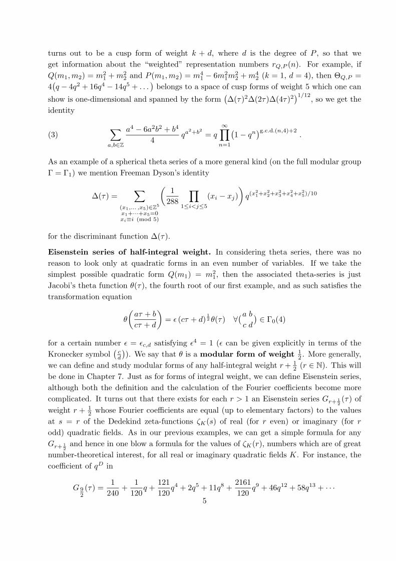
turns out to be a cusp form of weight k + d, where d is the degree of P , so that we
get information about the “weighted” representation numbers rQ,P (n). For example, if
Q(m1,m2) = m21 +m2
2 and P (m1,m2) = m41 − 6m2
1m22 +m4
2 (k = 1, d = 4), then ΘQ,P =
4(q − 4q2 + 16q4 − 14q5 + . . .
)belongs to a space of cusp forms of weight 5 which one can
show is one-dimensional and spanned by the form(∆(τ)2∆(2τ)∆(4τ)2
)1/12, so we get the
identity
(3)∑
a,b∈Z
a4 − 6a2b2 + b4
4qa
2+b2 = q
∞∏
n=1
(1− qn
)g.c.d.(n,4)+2.
As an example of a spherical theta series of a more general kind (on the full modular group
Γ = Γ1) we mention Freeman Dyson’s identity
∆(τ) =∑
(x1,... ,x5)∈Z5
x1+···+x5=0xi≡i (mod 5)
(1
288
∏
1≤i<j≤5
(xi − xj)
)q(x
2
1+x2
2+x2
3+x2
4+x2
5)/10
for the discriminant function ∆(τ).
Eisenstein series of half-integral weight. In considering theta series, there was no
reason to look only at quadratic forms in an even number of variables. If we take the
simplest possible quadratic form Q(m1) = m21, then the associated theta-series is just
Jacobi’s theta function θ(τ), the fourth root of our first example, and as such satisfies the
transformation equation
θ
(aτ + b
cτ + d
)= ǫ (cτ + d)
1
2 θ(τ) ∀(ac
b
d
)∈ Γ0(4)
for a certain number ǫ = ǫc,d satisfying ǫ4 = 1 (ǫ can be given explicitly in terms of the
Kronecker symbol(cd
)). We say that θ is a modular form of weight 1
2 . More generally,
we can define and study modular forms of any half-integral weight r+ 12 (r ∈ N). This will
be done in Chapter 7. Just as for forms of integral weight, we can define Eisenstein series,
although both the definition and the calculation of the Fourier coefficients become more
complicated. It turns out that there exists for each r > 1 an Eisenstein series Gr+ 1
2
(τ) of
weight r + 12 whose Fourier coefficients are equal (up to elementary factors) to the values
at s = r of the Dedekind zeta-functions ζK(s) of real (for r even) or imaginary (for r
odd) quadratic fields. As in our previous examples, we can get a simple formula for any
Gr+ 1
2
and hence in one blow a formula for the values of ζK(r), numbers which are of great
number-theoretical interest, for all real or imaginary quadratic fields K. For instance, the
coefficient of qD in
G 92(τ) =
1
240+
1
120q +
121
120q4 + 2q5 + 11q8 +
2161
120q9 + 46q12 + 58q13 + · · ·
5

is135D7/2
2π8ζK(4) if D (= 5, 8, 12, . . . ) is the discriminant of a real quadratic field K; on
the other hand, on comparing G9/2 with the modular form G4(4τ)θ(τ) of the same weight
we find that they are equal and hence that we have the closed formula
ζK(4) =2π8
135D3√D
∑
|m|<√D
m2≡D (mod 4)
σ3(D −m2
4
)(D = discriminant of K)
for every real quadratic field K, a fairly deep result which it is much harder to prove
directly. For r = 1 the function G3/2 has coefficients which are the class numbers of
imaginary quadratic fields. Like G2, it is no longer quite modular but has a “nearly
modular” property which can be used to just as good effect. In this way also class numbers
can be brought into the theory of modular forms, most notably in connection with the
Eichler-Selberg formula for traces of Hecke operators (Chapter 8).
New forms from old. There are various methods which can be used to manufacture new
modular forms out of previously constructed ones. The first and most obvious method is
multiplication: the product of a modular form of weight k and one of weight l is a modular
form of weight k + l. Of course we have already used this above when we compared G24
and G8 or when we expressed ∆ as a linear combination of G34 and G2
6. The multiplicative
property of modular forms means that the set M∗ =⊕Mk of all modular forms on Γ1
forms a graded ring. We will see in Chapter 1 that it in fact coincides with the ring of all
polynomials in G4 and G6.
More interesting structures, which we will also study in Chapter 1, are connected with
the possibility of obtaining new modular forms by combining derivatives of modular forms
of lower weight. Given two modular forms f and g of weight k and l, respectively, there
is for each positive integer ν a combination of the products of derivatives f (i)(τ)g(ν−i)(τ))
(0 ≤ i ≤ ν) which is a cusp form of weight k + l + 2ν. For instance (k = 4, l = 6, ν = 1),
the function 2G4(τ)G′6(τ)− 3G′
4(τ)G6(τ) is a cusp form of weight 12 and hence, since the
space of such cusp forms is 1-dimensional, a multiple of ∆. More generally, we will see that
the “extended” ring of modular forms generated by G4, G6, and the “near”-modular form
G2 is closed under differentiation, with the consequence that any modular form satisfies a
non-linear third-order differential equation.
Finally, we can get new modular forms from old ones by looking at combinations of the
functions (cτ +d)−kf(aτ+bcτ+d
)(“slash operator”), where f is a modular form of weight k and
γ =(acbd
)a 2×2 matrix with rational coefficients. Examples are the operators f(τ) 7→ f(aτ)
(like the functions G4(2τ) and G4(4τ) used above in connection with θ(τ)8) and the Hecke
operators which were mentioned in connection with the function ∆(τ).
Modular forms coming from algebraic geometry and number theory. Certain
power series∑a(n)qn whose coefficients a(n) are defined by counting the number of points
of algebraic varieties over finite fields are known or conjectured to be modular forms. For6
example, the famous “Taniyama-Weil conjecture” says that to any elliptic curve defined
over Q there is associated a modular form∑a(n)qn of weight 2 on some group Γ0(N)
such that p + 1 − a(p) for every prime number p is equal to the number of points of the
elliptic curve over Fp (e.g., to the number of solutions of x3 − ky3 ≡ 1 modulo p, where
k is a fixed integer). Of course, this cannot really be considered as a way of constructing
modular forms, since one can usually only prove the modularity of the function in question
if one has an independent, analytic construction of it. The Taniyama-Weil conjecture is
very deep and in particular is known to imply Fermat’s last theorem!
In a similar vein, one can get modular forms from algebraic number theory by looking at
Fourier expansions∑a(n)qn whose associated Dirichlet series
∑a(n)n−s are zeta functions
coming from number fields or their characters. For instance, a theorem of Deligne and Serre
says that one can get all modular forms of weight 1 in this way from the Artin L-series of
two-dimensional Galois representations with odd determinant satisfying Artin’s conjecture
(that the L-series is holomorphic). Again, however, the usual way of applying such a result
is to construct the modular form independently and then deduce that the corresponding
Artin L-series satisfies Artin’s conjecture.
In one situation, the situation of so-called “CM” (complex multiplication) forms, the
analytic, algebraic geometric, and number theoretic approaches come together: analytically,
these are the theta series ΘQ,P associated to a binary quadratic form Q and an arbitrary
spherical function P on Z2; geometrically, they arise from elliptic curves having complex
multiplication (i.e., non-trivial endomorphisms); and number theoretically, they are given
by Fourier developments whose associated Dirichlet series are the L-series of algebraic
Hecke grossencharacters over an imaginary quadratic field. An example is the function (3)
above. The characteristic property of CM forms is that they have highly lacunary Fourier
developments, because binary quadratic forms represent only a thin subset of all integers
(at most O(x/(log x)1/2
)integers ≤ x).
Modular forms in several variables. Finally, modular forms in one variable can be
obtained by restricting in some way different kinds of modular forms in more than one
variable (Jacobi, Hilbert, Siegel, . . . ), these in turn being constructed by the appropriate
generalization of one of the methods described above. Such forms will be discussed in Part
II.
Exercises
1. Check that the expression ℑ(τ)k/2|f(τ)| for a function f : H → C satisfying (1) is
invariant under τ 7→ (aτ + b)/(cτ + d).
2. Show that the group Γ1 is generated by the elements T =(1011
)and S =
(01−10
). (Hint:
Show that a2+b2+c2+d2 for a matrix γ =(acbd
)6= ±I2 in Γ1 can be reduced by multiplying
γ on the right by STn for a suitable integer n.) Deduce that a function f : H → C belongs
to Mk(Γ1) if and only if it has a convergent Fourier expansion f(τ) =∑∞
n=0 a(n) e2πinτ
and satisfies the functional equation f(−1/τ) = τkf(τ).7
3. Show that if f(τ) is a modular form of weight k on Γ1 then f(rτ) is a modular form
of weight k on Γ0(N) for any positive integers r and N with N divisible by r.
4*. Give an elementary proof of (2).
8

Chapter 1. Modular Forms on SL2(Z)
In this chapter we study the space of modular forms on the full modular group Γ1 =
SL2(Z) . In particular, we prove the modularity properties of the Eisenstein series Gk
and discriminant function ∆ mentioned in Chapter 0, describe the structure of the ring
of modular forms, and discuss the modularity properties of derivatives of modular forms.
Many of the ideas (e.g., the construction of Eisenstein series) go through almost unchanged
for other groups Γ, but restricting attention to Γ1 we can simplify many of the details and
give more complete results.
1.1. Eisenstein series. Recall that a modular form of weight k on Γ1 is a function
f : H → C having a Fourier expansion f(τ) =∑∞
n=0 a(n) qn (q = e2πiτ ) which converges
for all τ ∈ H and satisfying the modular transformation property
(1) f(γτ
)= (cτ + d)k f(τ)
(∀γ =
(ac
b
d
)∈ Γ1, γτ =
aτ + b
cτ + d
)
By Exercise 2 of Chapter 0, it is enough to require (1) for the matrix γ =(01−10
)only.
The first construction of such a form is a very simple one, but already here the Fourier
coefficients will turn out to give interesting arithmetic functions. For k even and greater
than 2, define the Eisenstein series of weight k by
(2) Gk(τ) =(k − 1)!
2(2πi)k
∑′
m,n
1
(mτ + n)k,
where the sum is over all pairs of integers (m,n) except (0, 0). (The reason for the normaliz-
ing factor (k−1)!/2(2πi)k, which is not always included in the definition, will become clear
in a moment.) This transforms like a modular form of weight k because replacing Gk(τ)
by (cτ + d)−kGk(aτ+bcτ+d ) simply replaces (m,n) by (am+ cn, bm+ dn) and hence permutes
the terms of the sum. We need the condition k > 2 to guarantee the absolute convergence
of the sum (and hence the validity of the argument just given) and the condition k even
because the series with k odd are identically zero (the terms (m,n) and (−m,−n) cancel).To see that Gk satisfies the growth condition defining Mk, and to have our first example
of an arithmetically interesting modular form, we must compute the Fourier development.
We begin with the Lipschitz formula
∑
n∈Z
1
(z + n)k=
(−2πi)k
(k − 1)!
∞∑
r=1
rk−1e2πirz (k ∈ Z≥2, z ∈ H),
which is proved in Appendix A1. Splitting the sum defining Gk into the terms with m = 0
and the terms with m 6= 0, and using the evenness of k to restrict to the terms with n
positive in the first and m positive in the second case, we find
Gk(τ) =(k − 1)!
(2πi)k
∞∑
n=1
1
nk+
∞∑
m=1
((k − 1)!
(2πi)k
∑
n∈Z
1
(mτ + n)k
)
=(−1)k/2(k − 1)!
(2π)kζ(k) +
∞∑
m=1
∞∑
r=1
rk−1e2πirmτ ,
9

where ζ(s) =∞∑
n=1
1
nsis Riemann’s zeta function. The number (−1)k/2(k−1)!
(2π)kζ(k) is rational
and in fact equals −Bk
2k, where Bk denotes the kth Bernoulli number (= coefficient of
xk
k!in the Taylor expansion of
x
ex − 1around x = 0); it is also equal to 1
2ζ(1 − k), where the
definition of ζ(s) is extended to negative s by analytic continuation (cf. Appendix A2).
Putting this into the formula for Gk and collecting for each n the terms with rm = n, we
find finally
(3) Gk(τ) = −Bk
2k+
∞∑
n=1
σk−1(n) qn =
1
2ζ(1− k) +
∞∑
n=1
σk−1(n) qn,
where σk−1(n) as in Chapter 0 denotes∑
r|n rk−1 (sum over all positive divisors r of n) and
we have again used the abbreviation q = e2πiτ . The beginnings of the Fourier developments
of G4, G6 and G8 were given in Chapter 0; the Fourier expansions of G10, G12, G14 and
G16 begin
G10(τ) = − 1
264+ q + 513q2 + · · · , G12(τ) =
691
65520+ q + 2049q2 + · · · ,
G14(τ) = − 1
24+ q + 8193q2 + · · · , G16(τ) =
3617
8160+ q + 32767q2 + · · ·
The fact that the Fourier coefficients occurring are all rational numbers is a special case of
the phenomenon that Mk in general is spanned by forms with rational Fourier coefficients.
It is this phenomenon which is responsible for the richness of the arithmetic applications
of the theory of modular forms.
The right-hand side of (3) makes sense also for k = 2 (B2 is equal to 16 ) and will be used
to define a function G2(τ). It is not a modular form (indeed, there can be no non-zero
modular form f of weight 2 on the full modular group, as we will see in the next section).
However, its transformation properties under the modular group can be easily determined
using Hecke’s trick: Define a function G∗2 by
G∗2(τ) =
−1
8π2limǫց0
(∑′
m,n
1
(mτ + n)2|mτ + n|ǫ).
The absolute convergence of the expression in parentheses for ǫ > 0 shows that G∗2 trans-
forms according to (1) (with k = 2), while applying the Poisson summation formula to this
expression first and then taking the limit ǫց 0 leads to the Fourier development
(4) G∗2(τ) = G2(τ) +
1
8πv(τ = u+ iv ∈ H).
The fact that the non-holomorphic function G∗2 transforms like a modular form of weight
2 then implies that the holomorphic function G2 transforms according to
(5) G2(aτ + b
cτ + d) = (cτ + d)2G2(τ)−
c(cτ + d)
4πi
((ac
b
d
)∈ Γ1
).
10

1.2. The discriminant function. We define a function ∆ in H by
(6) ∆(τ) = q∞∏
r=1
(1− qr)24 (τ ∈ H, q = e2πiτ ).
Then
∆′(τ)
∆(τ)=
d
dτ
(2πiτ + 24
∞∑
r=1
log(1− qr)
)
= 2πi
(1 − 24
∞∑
r=1
rqr
1− qr
)
= −48πi
(− 1
24+
∞∑
n=1
(∑
r|nr)qn
)= −48πiG2(τ).
The transformation formula (5) gives
1
(cτ + d)2∆′(aτ+b
cτ+d )
∆(aτ+bcτ+d )
=∆′(τ)
∆(τ)+ 12
c
cτ + d
ord
dτ
(log∆
(aτ + b
cτ + d
))=
d
dτlog
(∆(τ)(cτ + d)12
).
Integrating, we deduce that ∆(aτ+bcτ+d ) equals a constant times (cτ + d)12∆(τ). Moreover,
this constant must always be 1 since it is 1 for the special matrices(acbd
)=
(1011
)(compare
Fourier developments!) and(acbd
)=
(01−10
)(take τ = i !) and these matrices generate Γ1.
Thus ∆(τ) satisfies equation (1) with k = 12. Multiplying out the product in (6) gives the
expansion
(7) ∆(τ) = q − 24q2 + 252q3 − 1472q4 + 4830q5 − 6048q6 + 8405q7 − · · ·
in which only positive exponents of q occur. Hence ∆ is a cusp form of weight 12. The
coefficient of qn in the expansion (7) is usually denoted τ(n) and called the Ramanujan
function; as already mentioned in Chapter 0, it is a multiplicative function of n.
Using ∆, we can determine the space of modular forms of all weights. Indeed, there
can be no non-constant modular form of weight 0 (it would be a non-constant holomorphic
function on the compact Riemann surface H/Γ1 ∪ {∞}), and it follows that there can be
no non-zero modular form of negative weight (if f had weight m < 0, then f12∆|m| would
have weight 0 and a Fourier expansion with no constant term). Also, Mk = {0} for k odd
(take a = d = −1, b = c = 0 in (1)). Furthermore, the space M2 is also trivial, since if
f(τ) were an element of M2 then f(τ) dτ would be a meromorphic differential form on the
Riemann surface H/Γ1 ∪ {∞} of genus 0 with a single pole of order ≤ 1, contradicting the
residue theorem. (For a less fancy version of this argument, see Exercise 2.) For k even and11
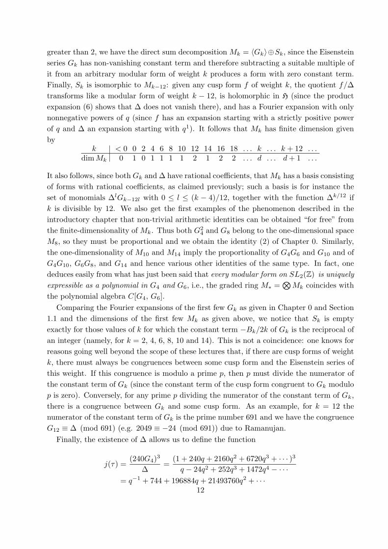
greater than 2, we have the direct sum decompositionMk = 〈Gk〉⊕Sk, since the Eisenstein
series Gk has non-vanishing constant term and therefore subtracting a suitable multiple of
it from an arbitrary modular form of weight k produces a form with zero constant term.
Finally, Sk is isomorphic to Mk−12: given any cusp form f of weight k, the quotient f/∆
transforms like a modular form of weight k − 12, is holomorphic in H (since the product
expansion (6) shows that ∆ does not vanish there), and has a Fourier expansion with only
nonnegative powers of q (since f has an expansion starting with a strictly positive power
of q and ∆ an expansion starting with q1). It follows that Mk has finite dimension given
byk < 0 0 2 4 6 8 10 12 14 16 18 . . . k . . . k + 12 . . .
dimMk 0 1 0 1 1 1 1 2 1 2 2 . . . d . . . d+ 1 . . .
It also follows, since both Gk and ∆ have rational coefficients, thatMk has a basis consisting
of forms with rational coefficients, as claimed previously; such a basis is for instance the
set of monomials ∆lGk−12l with 0 ≤ l ≤ (k − 4)/12, together with the function ∆k/12 if
k is divisible by 12. We also get the first examples of the phenomenon described in the
introductory chapter that non-trivial arithmetic identities can be obtained “for free” from
the finite-dimensionality ofMk. Thus both G24 and G8 belong to the one-dimensional space
M8, so they must be proportional and we obtain the identity (2) of Chapter 0. Similarly,
the one-dimensionality of M10 and M14 imply the proportionality of G4G6 and G10 and of
G4G10, G6G8, and G14 and hence various other identities of the same type. In fact, one
deduces easily from what has just been said that every modular form on SL2(Z) is uniquely
expressible as a polynomial in G4 and G6, i.e., the graded ring M∗ =⊗Mk coincides with
the polynomial algebra C[G4, G6].
Comparing the Fourier expansions of the first few Gk as given in Chapter 0 and Section
1.1 and the dimensions of the first few Mk as given above, we notice that Sk is empty
exactly for those values of k for which the constant term −Bk/2k of Gk is the reciprocal of
an integer (namely, for k = 2, 4, 6, 8, 10 and 14). This is not a coincidence: one knows for
reasons going well beyond the scope of these lectures that, if there are cusp forms of weight
k, there must always be congruences between some cusp form and the Eisenstein series of
this weight. If this congruence is modulo a prime p, then p must divide the numerator of
the constant term of Gk (since the constant term of the cusp form congruent to Gk modulo
p is zero). Conversely, for any prime p dividing the numerator of the constant term of Gk,
there is a congruence between Gk and some cusp form. As an example, for k = 12 the
numerator of the constant term of Gk is the prime number 691 and we have the congruence
G12 ≡ ∆ (mod 691) (e.g. 2049 ≡ −24 (mod 691)) due to Ramanujan.
Finally, the existence of ∆ allows us to define the function
j(τ) =(240G4)
3
∆=
(1 + 240q + 2160q2 + 6720q3 + · · · )3q − 24q2 + 252q3 + 1472q4 − · · ·
= q−1 + 744 + 196884q + 21493760q2 + · · ·12
and see (since G34 and ∆ are modular forms of the same weight on Γ1) that it is invariant
under the action of Γ1 on H. Conversely, if φ(τ) is any modular function on H which grows
at most exponentially as ℑ(τ) → ∞, then the function f(τ) = φ(τ)∆(τ)m transforms like
a modular form of weight 12m and (if m is large enough) is bounded at infinity, so that
f ∈M12m; by what we saw above, f is then a homogeneous polynomial of degree m in G34
and ∆, so φ = f/∆m is a polynomial of degree ≤ m in j. This justifies calling j(τ) “the”
modular invariant function. In fact, we can say more. Define a subset F of H as the set of
τ = u + iv satisfying |u| ≤ 12 , |τ | ≥ 1. Using Exercise 2 of Chapter 0, one can show that
every point of H can be mapped by an element of Γ1 to a point of F . If f is a modular
form of weight k which does not vanish at infinity (i.e., has constant term a(0) 6= 0) or
anywhere on the boundary ∂F of F , then by integrating f ′(τ)/f(τ) around ∂F we find
that f has exactly k/12 zeroes in the interior of F (in particular, k must be divisible by
12; modular forms on Γ1 must have zeroes on the boundary of F and more specifically
at the point i if 4 6 |k and at the points (±1 + i√3)/2 if 3 6 |k, as one sees by applying a
variant of the same argument or directly as in Exercise 3). In particular, for each λ ∈ C the
function (240G4)3 − λ∆(τ) has exactly one zero in the interior of F if it does not vanish
on ∂F . This shows that j(τ) gives an isomorphism from the Riemann surface X obtained
by identifying the edges of F via τ ∼ τ +1 for u = − 12 and τ ∼ −1/τ for |τ | = 1 to the set
of complex numbers. Alternatively, one can observe that the function j − λ on the closed
surface obtained by adding a “point at infinity” to X has exactly one pole, at infinity, and
hence exactly one zero, at some finite point. It follows that any meromorphic function on H
which is Γ1-invariant and grows at most exponentially in v = ℑ(τ) as v → ∞ is a rational
function of j(τ).
1.3. Modular forms and differential operators. The process of differentiation dis-
turbs the property of modularity. If we start with a function f satisfying (1), then we find
by differentiation that the derivative f ′ satisfies the equation
(8) f ′(aτ + b
cτ + d
)= (cτ + d)k+2 f ′(τ) + kc(cτ + d)k+1 f(τ) ,
i.e., it behaves nearly like a modular form of weight k + 2 but with a slight perturbation.
There are two ways to get around this difficulty and produce modular forms of higher
weight by a differentiation property. The first is to combine derivatives of two different
modular forms. For instance, if g ∈ Ml is a second modular form, then writing down the
analogue of (8) for g we see that the perturbations of the modularity property of f ′(τ)g(τ)
and of f(τ)g′(τ) are the same up to a factor k/l and hence that the function
(9) F1(f, g)(τ) =1
2πi
(l f ′(τ) g(τ)− k f(τ) g′(τ)
)
is a modular form (in fact, a cusp form, since the constant term is obviously zero) of weight
k + l + 2. As the simplest numerical example, the function F1(G4, G6) = − 135q − · · · is a
13

cusp form of weight 12 and hence equals − 135∆, which gives the formula
τ(n) =5σ3(n) + 7σ5(n)
12n − 35
∑
a,b>0a+b=n
(6a− 4b)σ3(a)σ5(b)
for the coefficient τ(n) of qn in ∆. The operation F1 is antisymmetric in its two arguments
and satisfies the Jacobi identity, so that it makes M∗−2 =⊕nMn−2 into a graded Lie
algebra. More generally, for each ν > 0 we have H. Cohen’s differential operator Fν
which is defined for f ∈Mk, g ∈Ml by
(10) Fν(f, g)(τ) = (2πi)−νν∑
µ=0
(−1)µ(k + ν − 1
µ
)(l + ν − 1
ν − µ
)f (ν−µ)(τ) g(µ)(τ)
(the normalization has been chosen so that Fν(f, g) has integral Fourier coefficients if both
f and g do). We claim that this is a modular form (and hence again a cusp form, as for
ν = 1) of weight k + l + 2ν. To see this, first prove the generalization
(11) f (µ)(aτ + b
cτ + d
)=
µ∑
λ=0
µ!(k + µ− 1)!
λ!(µ− λ)!(k + λ− 1)!cµ−λ(cτ + d)k+µ+λf (λ)(τ)
of (8) by induction on µ. These transformation formulas can be combined into the single
statement that the generating function
(12) f(τ,X) =∞∑
µ=0
1
µ!(k + µ− 1)!f (µ)(τ)Xµ (τ ∈ H, X ∈ C)
satisfies
(13) f(aτ + b
cτ + d,
X
(cτ + d)2)= (cτ + d)k ecX/(cτ+d) f(τ,X) (
(ac
b
d
)∈ Γ).
From this and the corresponding formula for g it follows that the product
f(τ,X) g(τ,−X) =∞∑
ν=0
(2πi)ν
(ν + k − 1)!(ν + l − 1)!Fν(f, g)(τ)X
ν
is multiplied by (cτ+d)k+l when τ and X are replaced by aτ+bcτ+d and X
(cτ+d)2 , and this proves
the modular transformation property of Fν(f, g) for every ν. The differential operators Fν
have many applications in the theory of modular forms, some of which will be described in
later chapters. As an example, we mention that the generalized theta series with spherical
polynomial coefficients ΘQ,P mentioned in Chapter 0 can be obtained from the simpler
theta series ΘQ by the use of these operators, e.g. if θ(τ) =∑qn
2
is the basic theta-series
of weight 12 on Γ0(4), then
23F2(θ, θ) is the function occurring in equation (3) of Chapter 0.
14
The second way around the problem caused by the extra term in (8) involves the near-
modular form G2 of Section 1.1. Comparing the transformation equations (5) and (8),
we find that for any f ∈ Mk the function f ′(τ) + 4πikG2(τ)f(τ) belongs to Mk+2. For
instance, for the two forms G4 and G6 we have
(14)1
2πiG′
4(τ) =7
10G6(τ)−8G2(τ)G4(τ),
1
2πiG′
6(τ) =10
21G8(τ)−12G2(τ)G6(τ) .
Similarly, by differentiating (3) we find that G′2(τ) + 4πiG2(τ)
2 belongs to M4, whence
(15)1
2πiG′
2(τ) =5
6G4(τ)− 2G2(τ)
2 .
The formulas (14) and (15) imply that the extension C[G2, G4, G6] of the ring M∗ =
C[G4, G6] is closed under differentiation. It follows that if a function f belongs to this
ring, then so do the functions f ′, f ′′ and f ′′′ and (since the ring has only three generators)
these four functions must be algebraically dependent. In particular, G2 and all modular
forms on Γ1 satisfy third-order differential equations, e.g., iπ G
′′′2 − 48G2G
′′2 + 72G′
22= 0.
Exercises
1. Show that the series (2) converges absolutely for k > 2. (Hint: The number of pairs
(m,n) for which |mτ + n| lies between N and N +1 is bounded by a multiple of N , so the
series converges like∞∑
N=1
N
Nk.)
2. Prove that the spaceM2 is trivial. (Hint: Show that if f(τ) =∑∞
n=0 a(n)qn belongs to
M2 then the integrated function F (τ) = a(0)τ +∑∞
n=1 a(n)qn/2πin would be Γ1-invariant
up to a constant, i.e., F (γ(τ)) = F (τ) + C(γ) for all τ ∈ H and γ ∈ Γ1 for some constant
C(γ). The map C : Γ1 → C would be a homomorphism and hence 0 since Γ1 is generated
by the elements S and ST of finite order, where S and T are defined as in Exercise 2 of
Chapter 0.)
3. Show that a modular form of weight k on Γ1 vanishes at i if 46 |k and at (±1+ i√3)/2
if 36 |k (hint: apply (1) with γ = S or ST ).
4. Check the various claims made in the final paragraph of §1.2.5. Check the formula (11) and the other steps in the proof of the modularity of Fν(f, g).
15

Chapter 2. Hecke Theory
The key to the rich internal structure of the theory of modular forms is the existence
of a commutative algebra of operators Tn (n ∈ N) acting on the space Mk of modular
forms of weight k. The space Mk has a canonical basis of simultaneous eigenvectors of all
the Tn; these special modular forms have the property that their Fourier coefficients a(n)
are algebraic integers and satisfy the multiplicative property a(nm) = a(n)a(m) whenever
n and m are relatively prime. In particular, their associated Dirichlet series∑a(n)n−s
have Euler products; they also have analytic continuations to the whole complex plane and
satisfy functional equations analogous to that of the Riemann zeta function. We will define
the operators Tn in Section 2.1 and describe their eigenforms and the associated Dirichlet
series in Sections 2.2 and 2.3, respectively. The final section of the chapter describes the
modifications of the theory for modular forms on subgroups of SL2(Z) .
2.1. Hecke operators. At the beginning of Chapter 0 we introduced the notion of
modular forms of higher weight by giving a bijection
(1)F (Λ) 7→ f(τ) = F (Zτ + Z),
f(τ) 7→ F (Λ) = ω−k2 f(ω1/ω2) (Λ = Zω1 + Zω2, ℑ(ω1/ω2) > 0)
between functions f in the upper half-plane transforming like modular forms of weight k
and functions F of lattices Λ ⊂ C which are homogeneous of weight −k, F (λΛ) = λ−kF (Λ).
If we fix a positive integer n, then every lattice Λ has a finite number of sublattices Λ′ of
index n, and we have an operator Tn on functions of lattices which assigns to such a function
F the new function
(2) TnF (Λ) = nk−1∑
Λ′⊆Λ
[Λ:Λ′]=n
F (Λ′)
(the factor nk−1 is introduced for convenience only). Clearly TnF is homogeneous of degree
−k if F is, so we can transfer the operator to an operator Tn on functions in the upper
half-plane which transform like modular forms of weight k. This operator is given explicitly
by
(3) Tnf(τ) = nk−1∑
(ac
bd
)∈Γ1\Mn
(cτ + d)−kf(aτ + b
cτ + d
)
and is called the nth Hecke operator in weight k; here Mn denotes the set of 2 × 2
integral matrices of determinant n and Γ1\Mn the finite set of orbits of Mn under left
multiplication by elements of Γ1 = SL2(Z) . Clearly this definition depends on k and we16
should more correctly write Tk(n)f or (the standard notation) f |kTn, but we will consider
the weight as fixed and write simply Tnf for convenience. In terms of the “slash operator”
(f |kγ)(τ) =(ad− bc)k/2
(cτ + d)kf(aτ + b
cτ + d
)(γ =
(ac
b
d
), a, b, c, d ∈ R, ad− bc > 0)
mentioned in Chapter 0, formula (3) can be expressed in the form
Tnf(τ) = nk2−1
∑
µ∈Γ1\Mn
f |kµ.
From the fact that |k is a group operation (i.e. f |k(γ1γ2) = (f |kγ1)|kγ2 for γ1, γ2 in
GL+2 (R)), we see that Tnf is well-defined (changing the orbit representative µ to γµ with
γ ∈ Γ1 doesn’t affect f |kµ because f |kγ = f) and again transforms like a modular form of
weight k on Γ1 ((Tnf)|kγ = Tnf for γ ∈ Γ1 because {µγ | µ ∈ Γ1\Mn} is another set of
representatives for Γ1\Mn). Of course, both of these properties are also obvious from the
invariant definition (2) and the isomorphism (1).
Formula (3) makes it clear that Tn preserves the property of being holomorphic. We
now give a description of the action of Tn on Fourier expansions which shows that Tn
also preserves the growth properties at infinity defining modular forms and cusp forms,
respectively, and also that the various Hecke operators commute with one another.
Theorem 1. (i) If f(τ) is a modular form with the Fourier expansion∞∑
m=0amq
m
(q = e2πiτ ), then the Fourier expansion of Tnf is given by
(4) Tnf(τ) =∞∑
m=0
( ∑
d|n,mdk−1 a
(nmd2
))qm,
where∑
d|n,m denotes a sum over the positive common divisors of n and m. In particular,
Tnf is again a modular form, and is a cusp form if f is one.
(ii) The Hecke operators in weight k satisfy the multiplication rule
(5) TnTm =∑
d|n,mdk−1 Tnm/d2 .
In particular, TnTm = TmTn for all n and m and TnTm = Tnm if n and m are coprime.
Proof. If µ =(acbd
)is a matrix of determinant n with c 6= 0, then we can choose a matrix
γ =(a′
c′b′
d′
)∈ SL2(Z) with
a′
c′=
a
c, and γ−1µ then has the form
(∗0∗∗). Hence we can
assume that the coset representatives in (3) have the form µ =(a0bd
)with ad = n, b ∈ Z.
A different choice γ(a0bd
)(γ ∈ SL2(Z) ) of representative also has this form if and only if
γ = ±(10r1
)with r ∈ Z, in which case γ
(a0bd
)= ±
(a0b+drd
), so the choice of µ is unique if
we require a, d > 0 and 0 ≤ b < d. Hence
Tnf(τ) = nk−1∑
a,d>0ad=n
d−1∑
b=0
d−k f(aτ + b
d
).
17

Substituting into this the formula f =∑a(m) qm gives (4) after a short calculation. The
second assertion of (i) follows from (4) because all of the exponents of q on the right-hand
side are ≥ 0 and the constant term equals a(0)σk−1(n) (σk−1(n) as in 1.1), so vanishes if
a(0) = 0. The multiplication properties (5) follow from (4) by another easy computation. �
In the special case when n = p is prime, the formula for the action of Tn reduces to
Tpf(τ) =1
p
p−1∑
j=0
f
(τ + j
p
)+ pk−1 f(pτ) =
∞∑
m=0
a(mp) qm + pk−1∞∑
m=0
a(m) qmp.
The multiplicative property (5) tells us that knowing the Tp is sufficient for knowing all Tn,
since if n > 1 is divisible by a prime p then Tn = Tn/pTp if p2 ∤ n, Tn = Tn/pTp−pk−1Tn/p2
if p2|n.To end this section, we remark that formula (4), except for the constant term, makes
sense also for n = 0, the common divisors of 0 and m being simply the divisors of m. Thus
the coefficient of qm on the right is just a(0)σk−1(m) for each m > 0. The constant term
is formally a(0)∑∞
d=1 dk−1 = a(0)ζ(1 − k), but in fact we take it to be 1
2a(0)ζ(1 − k) =
−a(0)Bk
2k. Thus we set
(6) T0f(τ) = a(0)Gk(τ) (f =
∞∑
m=0
a(m) qm ∈Mk);
in particular, T0 maps Mk to Mk and T0f = 0 if f is a cusp form.
2.2. Eigenforms. We have seen that the Hecke operators Tn act as linear operators on the
vector space Mk. Suppose that some modular form f(τ) =∞∑
m=0a(m) qm is an eigenvector
of all the Tn, i.e.,
(7) Tnf = λnf (∀n)
for some complex numbers λn. This certainly sometimes happens. For instance, if k = 4,
6, 8, 10 or 14, then the space Mk is 1-dimensional, spanned by the Eisenstein series Gk, so
TnGk is necessarily a multiple of Gk for every n. (Actually, we will see in a moment that
this is true even if dimMk > 1.) Similarly, if k = 12, 16, 18, 20, 22 or 26, then the space
Sk of cusp forms of weight k is 1-dimensional, and since Tn preserves Sk, any element of
Sk satisfies (7). From (7) and (4) we obtain the identity
(8) λn a(m) =∑
d|n,mdk−1 a
(nmd2
)
by comparing the coefficients of qm on both sides of (7). In particular, λna(1) = a(n) for
all n. It follows that a(1) 6= 0 if f is not identically zero, so we can normalize f by requiring18
that a(1) = 1. We call a modular form satisfying (7) and the extra condition a(1) = 1 a
Hecke form (the term “normalized Hecke eigenform” is commonly used in the literature).
From what we have just said, it follows that a Hecke form has the property
(9) λn = a(n) (∀n),
i.e., the Fourier coefficients of f are equal to its eigenvalues under the Hecke operators.
Equation (5) or (8) now implies the property
(10) a(n) a(m) =∑
d|n,mdk−1 a
(nmd2
)
for the coefficients of a Hecke form. In particular, the sequence of Fourier coefficients {a(n)}is multiplicative, i.e., a(1) = 1 and a(nm) = a(n)a(m) whenever n and m are coprime.
In particular, a(pr11 . . . prll ) = a(pr11 ) . . . a(prll ) for distinct primes p1, . . . , pl, so the a(n) are
determined if we know the values of a(pr) for all primes p. Moreover, (10) with n = pr,
m = p gives the recursion
(11) a(pr+1) = a(p) a(pr)− pk−1a(pr−1) (r ≥ 1)
for the coefficients a(pr) for a fixed prime p, so it in fact is enough to know the a(p)
(compare the remark following Theorem 1).
Examples. 1. The form Gk = −Bk
2k+
∞∑
m=1
σk−1(m) qm ∈Mk is a Hecke form for all k ≥ 4
with λn = a(n) = σk−1(n) for n > 0 and λ0 = a(0) = −Bk
2k(cf. (6)). In view of (4), to
check this we need only check that the coefficients a(n) of Gk satisfy (10) if n or m > 0;
this is immediate if n or m equals 0 and can be checked easily for n and m positive by
reducing to the case of prime powers (for n = pν , σk−1(n) equals 1 + pk−1 + · · ·+ pν(k−1),
which can be summed as a geometric series) and using the obvious multiplicativity of the
numbers σk−1(n).
2. The discriminant function ∆ discussed in 1.2 belongs to the 1-dimensional space S12
and has 1 as coefficient of q1, so it is a Hecke form. In particular, (10) holds (with k = 12)
for the coefficients a(n) of ∆, as we can check for small n using the coefficients given in (7)
of 1.2:
a(2)a(3) =−24× 252 =−6048 = a(6), a(2)2 = 576 =−1472 + 2048 = a(4) + 211.
This multiplicativity property of the coefficients of ∆ was noticed by Ramanujan in 1916
and proved by Mordell a year later by the same argument as we have just given.
The proof that ∆ is a simultaneous eigenform of the Tn used the property dimSk = 1,
which is false for k > 26. Nevertheless, there exist eigenforms in higher dimensions also;
this is Hecke’s great discovery. Indeed, we have:19

Theorem 2. The Hecke forms in Mk form a basis of Mk for every k.
Proof. We have seen that Gk is an eigenform of all Tn. Conversely, any modular form with
non-zero constant term which is an eigenform of all Tn (n ≥ 0) is a multiple of Gk by virtue
of equation (6) of Section 2.1. In view of this and the decomposition Mk = 〈Gk〉 ⊕ Sk, it
suffices to show that Sk is spanned by Hecke forms and that the Hecke forms in Sk are
linearly independent. For this we use the Petersson scalar product
(12) (f, g) =
∫∫
H/Γ1
vk f(τ) g(τ) dµ (f, g ∈ Sk),
where we have written τ as u+ iv and dµ for the measure v−2 du dv on H, and the integral
is taken over a fundamental domain for the action of Γ1 on H. This integral makes sense
because the function vk|f(τ)|2 and the measure dµ are both Γ1-invariant and converges
absolutely because vk|f(τ)|2 is bounded and∫H/Γ1
dµ < ∞. It gives Sk the structure of
a finite-dimensional Hilbert space. One checks from the definition (3) that the Tn are
self-adjoint with respect to this structure, i.e. (Tnf, g) = (f, Tng) for all f, g ∈ Sk and
n > 0. (For n = 0, of course, Tn is the zero operator on Sk by equation (6).) Also, the Tncommute with one another, as we have seen. A well-known theorem of linear algebra then
asserts that Sk is spanned by simultaneous eigenvectors of all the transformations Tn, and
we have already seen that each such eigenform is uniquely expressible as a multiple of a
Hecke form satisfying (10). Moreover, for a Hecke form we have
a(n) (f, f) = (a(n)f, f) = (λnf, f) = (Tnf, f)
= (f, Tnf) = (f, λnf) = (f, a(n)f) = a(n) (f, f)
by the self-adjointness of Tn and the sesquilinearity of the scalar product. Therefore the
Fourier coefficients of f are real. If g =∑b(n) qn is a second Hecke form in Sk, then the
same computation shows that
a(n) (f, g) = (Tnf, g) = (f, Tng) = b(n) (f, g) = b(n) (f, g)
and hence that (f, g) = 0 if f 6= g. Thus the various Hecke forms in Sk are mutually
orthogonal and a fortiori linearly independent. �
We also have
Theorem 3. The Fourier coefficients of a Hecke form f ∈ Sk are real algebraic integers
of degree ≤ dimSk.
Proof. The space Sk is spanned by forms all of whose Fourier coefficients are integral (this
follows easily from the discussion in Section 1.2. By formula (4), the lattice Lk of all such
forms is mapped to itself by all Tn. Let f1, . . . , fd (d = dimC Sk = rkZLk) be a basis for
Lk over Z. Then the action of Tn with respect to this basis is given by a d × d matrix20

with coefficients in Z, so the eigenvalues of Tn are algebraic integers of degree ≤ d. By (9),
these eigenvalues are precisely the Fourier coefficients of the d Hecke forms in Sk. That
the coefficients of Hecke forms are real was already checked in proving Theorem 2. �
From the proof of the theorem, we see that the trace of Tn (n > 0) acting on Mk or Sk
is the trace of a (d+ 1)× (d+ 1) or d× d matrix with integral coefficients and hence is an
integer. This trace is given in closed form by the Eichler-Selberg trace formula, which will
be discussed in Chapter 8.
Example. The space S24 is 2-dimensional, spanned by
∆(τ)2 = 0q + q2 − 48 q3 + 1080 q4 + · · ·
and
(240G4(τ))3 ∆(τ) = q + 696 q2 + 162252 q3 + 12831808 q4 + · · ·
If f ∈ S24 is a Hecke form, then f must have the form (240G4)3∆+ λ∆2 for some λ ∈ C,
since the coefficient of q1 must be 1. Hence its second and fourth coefficients are given by
a(2) = 696 + λ, a(4) = 12831808 + 1080λ.
The property a(2)2 = a(4) + 223 (n = m = 2 in (10)) now leads to the quadratic equation
λ2 + 312λ− 20736000 = 0
for λ. Hence any Hecke form in S24 must be one of the two functions
f1, f2 = (240G4)3 ∆+
(−156± 12
√144169
)∆2.
Since Theorem 2 says that S24 must contain exactly two Hecke forms, f1 and f2 are indeed
eigenvectors with respect to all the Tn. This means, for example, that we would have
obtained the same quadratic equation for λ if we had used the relation a(2)a(3) = a(6)
instead of a(2)2 = a(4) + 223. The coefficients a1(n), a2(n) of f1 and f2 are conjugate
algebraic integers in the real quadratic field Q(√144169).
2.3. L-series. The natural reflex of a number-theorist confronted with a multiplicative
function n 7→ a(n) is to form the Dirichlet series∞∑
n=1a(n)n−s, the point being that the
multiplicative property implies that a(pr11 . . . prll ) = a(pr11 ) . . . a(prll ) and hence that this
Dirichlet series has an Euler product∏
p prime
(∑r≥0
a(pr) p−rs). We therefore define theHecke
L-series of a modular form f(τ) =∑∞
m=0 a(m) qm ∈Mk by
(13) L(f, s) =
∞∑
m=1
a(m)
ms
21
(notice that we have ignored a(0) in this definition; what else could we do?). Thus if f is
a Hecke form we have an Euler product
L(f, s) =∏
p prime
(1 +
a(p)
ps+a(p2)
p2s+ · · ·
)
because the coefficients a(m) are multiplicative. But in fact we can go further, because the
recursion (11) implies that for each prime p the generating function Ap(x) =∑a(pr)xr
satisfies
Ap(x) = 1 +
∞∑
r=0
a(pr+1)xr+1 = 1 +
∞∑
r=0
a(p) a(pr)xr+1 −∞∑
r=1
pk−1 a(pr−1)xr+1
= 1 + a(p)xAp(x) − pk−1 x2Ap(x)
and hence that
Ap(x) =1
1− a(p)x+ pk−1x2.
Therefore, replacing x by p−s and multiplying over all primes p, we find finally
(14) L(f, s) =∏
p
1
1− a(p)p−s + pk−1−2s(f ∈Mk a Hecke form).
Examples. 1. For f = Gk we have
a(pr) = 1 + pk−1 + · · ·+ pr(k−1) =p(r+1)(k−1) − 1
pk−1 − 1,
Ap(x) =∞∑
r=0
p(r+1)(k−1) − 1
pk−1 − 1xr =
1(1− pk−1x
)(1− x
)
L(Gk, s) =∏
p
1
1− σk−1(p)p−s + pk−1−2s=
∏
p
1
(1− pk−1−s)(1− p−s)
= ζ(s− k + 1)ζ(s),
where ζ(s) is the Riemann zeta function. (Of course, we could see this directly: the
coefficient of n−s in ζ(s− k + 1)ζ(s) =∑
d,e≥1
dk−1
(de)sis clearly σk−1(n) for each n ≥ 1.)
2. For f = ∆ we have
L(∆, s) =∏
p
1
1− τ(p)p−s + p11−2s,
where τ(n), the Ramanujan tau-function, denotes the coefficient of qn in ∆; this identity
summarizes all the multiplicative properties of τ(n) discovered by Ramanujan.
Of course, the Hecke L-series would be of no interest if their definition were merely for-
mal. However, these series converge in a half-plane and define functions with nice analytic
properties, as we now show.22
Theorem 4. (i) The Fourier coefficients a(m) of a modular form of weight k satisfy the
growth estimates
(15) a(n) = O(nk−1
)(f ∈Mk), a(n) = O
(n
k2
)(f ∈ Sk).
Hence the L-series L(f, s) converges absolutely and locally uniformly in the half-plane
ℜ(s) > k, and in the larger half-plane ℜ(s) > k
2+ 1 if f is a cusp form.
(ii) L(f, s) has a meromorphic continuation to the whole complex plane. It is holo-
morphic everywhere if f is a cusp form and has exactly one singularity, a simple pole of
residue(2πi)k
(k − 1)!a(0) at s = k, otherwise. The meromorphically extended function satisfies
the functional equation
(2π)−s Γ(s)L(f, s) = (−1)k2 (2π)s−k Γ(k − s)L(f, k − s).
Proof. (i) Since the estimate a(n) = O(nk−1) is obvious for the Eisenstein series Gk (we
have σk−1(n) = nk−1∑
d|n d−k+1 < nk−1
∑∞d=1 d
−k+1 = ζ(k − 1)nk−1), and since every
modular form of weight k is a combination of Gk and a cusp form, we need only prove the
second estimate in (15). If f is a cusp form then by definition we have |f(τ)| < Mv−k/2
for some constant M > 0 and all τ = u + iv ∈ H. On the other hand, for any n ≥ 1 and
v > 0 we have
a(n) =
∫ 1
0
f(u+ iv) e−2πin(u+iv) du.
Hence
|a(n)| ≤M v−k/2 e2πnv,
and choosing v = 1/n gives the desired conclusion. (This argument, like most of the rest
of this chapter, is due to Hecke.)
(ii) This follows immediately from the “functional equation principle” in Appendix A2,
since the function
φ(v) = f(iv)− a(0) =
∞∑
n=1
a(n) e−2πnv (v > 0)
is exponentially small at infinity and satisfies the functional equation
φ(1v
)= f
(−1
iv
)− a(0) = (iv)k f(iv)− a(0) = (−1)
k2 vk φ(v) + (−1)
k2 a(0) vk − a(0)
and its Mellin transform∫∞0φ(v) vs−1 dv equals (2π)−sΓ(s)L(f, s). �
The first estimate in (15) is clearly best possible, but the second one can be improved.
The estimate a(n) = O(nk2− 1
5+ǫ) for the Fourier coefficients of cusp forms on Γ1 was found
by Rankin in 1939 as an application of the Rankin-Selberg method which will be discussed23

in Chapter 6. This was later improved to a(n) = O(nk2− 1
4+ǫ) by Selberg as an application
of Weil’s estimates of Kloosterman sums. The estimate
(16) a(n) = O(nk−1
2+ǫ) (f =
∑a(n) qn ∈ Sk),
conjectured by Ramanujan for f = ∆ in 1916 and by Petersson in the general case, remained
an open problem for many years. It was shown by Deligne in 1969 to be a consequence of the
Weil conjectures on the eigenvalues of the Frobenius operator in the l-adic cohomology of
algebraic varieties in positive characteristic; five years later he proved the Weil conjectures,
thus establishing (16). Using the form of the generating function Ap(x) given above, one
sees that (16) is equivalent to
(17) |a(p)| ≤ 2p(k−1)/2 (p prime).
In particular, for the Ramanujan tau-function τ(n) (coefficient of qn in ∆) one has
(18) |τ(p)| ≤ 2p11/2 (p prime).
Deligne’s proof of (18) uses the full force of Grothendieck’s work in algebraic geometry and
its length, if written out from scratch, has been estimated at 2000 pages; in his book on
mathematics and physics, Manin cites this as a probable record for the ratio “length of
proof : length of statement” in the whole of mathematics.
2.4. Forms of higher level. In these notes, we usually restrict attention to the full
modular group Γ1 = SL2(Z) rather than subgroups because most aspects of the theory
can be seen there. However, in the case of the theory of Hecke operators there are some
important differences, which we now describe. We will discuss only the subgroups Γ0(N) =
{(acbd
)∈ Γ1 | c ≡ 0 (mod N)} which were already introduced in Chapter 0.
First of all, the definition of Tn must be modified. In formula (3) we must replace Γ1
by Γ = Γ0(N) and Mn by the set of integral matrices(acbd
)of determinant n satisfying
c ≡ 0 (mod N) and (a,N) = 1. Again the coset representatives of Γ\Mn can be chosen
to be upper triangular, but the extra condition (a,N) = 1 means that we have fewer
representatives than before if (n,N) > 1. In particular, for p a prime dividing N we have
Tpf(τ) =∑a(mp)qm and Tpr = (Tp)
r rather than the more complicated formulas given in
the remark following Theorem 1 in 2.1; more generally, for n arbitrary the operation of Tn
is given by the same formula (4) as before but with the extra condition (d,N) = 1 added
to the inner sum, and similarly for the multiplicativity relation (5).
The other main difference with the case N = 1 comes from the existence of so-called
“old forms.” If N ′ is a proper divisor of N , then Γ0(N) is a subgroup of Γ0(N′) and every
modular form f(τ) of weight k on Γ0(N′) is a fortiori a modular form on Γ0(N). More
generally, f(Mτ) is a modular form of weight k on Γ0(N) for each positive divisor M of24

N/N ′, since
(ac
b
d
)∈ Γ0(N) ⇒
( a
c/M
bM
d
)∈ Γ0(N
′)
⇒ f(M
aτ + b
cτ + d
)= f
( a(Mτ) + bM
(c/M)(Mτ) + d
)= (cτ + d)kf(Mτ).
The subspace of Mk(Γ0(N)) spanned by all forms f(Mτ) with f ∈ Mk(Γ0(N′)), MN ′|N ,
N ′ 6= N , is called the space of old forms. (This definition must be modified slightly if
k = 2 to include also the modular forms∑
M |N cMG∗2(Mτ) with cM ∈ C,
∑M |N M−1cM =
0, where G∗2 is the non-holomorphic Eisenstein series of weight 2 on Γ1 introduced in
1.1, as old forms, even though G∗2 itself is not in M2(Γ1).) Since the old forms can be
considered by induction on N as already known, one is interested only in the “rest” of
Mk(Γ0(N)). The answer here is quite satisfactory: Mk(Γ0(N)) has a canonical splitting as
the direct sum of the subspace Mk(Γ0(N))old of old forms and a certainly complementary
space Mk(Γ0(N))new (for cusp forms, Sk(Γ0(N))new is just the orthogonal complement of
Sk(Γ0(N))old with respect to the Petersson scalar product), and if we define a Hecke form
of level N to be a form in Mk(Γ0(N))new which is an eigenvector of Tn for all n prime
to N and with a(1) = 1, then the Hecke forms are in fact eigenvectors of all the Tn, they
form a basis of Mk(Γ0(N))new, and their Fourier coefficients are real algebraic integers as
before. For the pth Fourier coefficient (p prime) of a Hecke form in Sk(Γ0(N))new we have
the same estimate (15) as before if p ∤ N , while the eigenvalue with respect to Tp when
p|N equals 0 if p2|N and ±p(k−2)/2 otherwise. Finally, there is no overlapping between the
newforms of different level or between the different lifts f(Mτ) of forms of the same level,
so that we have a canonical direct sum decomposition
Mk(Γ0(N)) =⊕
MN ′|N
{f(Mτ) | f ∈Mk(Γ0(N
′))new}
and a canonical basis of Mk(Γ0(N)) consisting of the functions f(Mτ) where M |N and f
is a Hecke form of some level N ′ dividing N/M .
As already stated, the Fourier coefficients of Hecke forms of higher level are real algebraic
integers, just as before. However, there is a difference with the case N = 1. For forms of
level 1, Theorem 3 apparently always is sharp: in all cases which have been calculated, the
number field generated by the Fourier coefficients of a Hecke cusp form of weight k has
degree equal to the full dimension d of the space Sk, which is then spanned by a single
form and its algebraic conjugates (cf. the example k = 24 given above). For forms of higher
level, on the other hand, there are in general further splittings. The general situation is
that Sk(Γ0(N))new splits as the sum of subspaces of some dimensions d1, . . . , dr ≥ 1, each
of which is spanned by some Hecke form, with Fourier coefficients in a totally real number
field Ki of degree di over Q, and the algebraic conjugates of this form (i.e. the forms
obtained by considering the various embeddings Ki → R). In general the number r and25

the dimensions di are unknown; the known theory implies certain necessary splittings of
Sk(Γ0(N))new, but there are often further splittings which we do not know how to predict.
Examples. 1. k = 2, N = 11. Here dimMk(Γ0(N)) = 2. As well as one old form, the
Eisenstein series
G∗2(τ)− 11G∗
2(11τ) =5
12+
∞∑
n=1
(∑
d|n11∤d
d
)qn
of weight 2, there is one new form
f(τ) = 12√∆(τ)∆(11τ) = q − 2q2 − q3 + 2q4 + q5 + 2q6 − 2q7 + · · · ,
with Fourier coefficients in Z. This form corresponds as in the Taniyama-Weil conjecture
mentioned in Chapter 0 to the elliptic curve y2 − y = x3 − x2, i.e., the number of solutions
of y2 − y = x3 − x2 in integers modulo p is given by p− a(p) for every prime p.
2. k = 2, N = 23. Again Mk(Γ0(N))old is 1-dimensional, spanned by G∗2(τ)−NG∗
2(Nτ),
but this time Mk(Γ0(N))new = Sk(Γ0(N))new is 2-dimensional, spanned by the Hecke form
f1 = q − 1−√5
2q2 +
√5 q3 − 1 +
√5
2q4 − (1−
√5) q5 − 5−
√5
2q6 + · · ·
with coefficients in Z+ Z1 +
√5
2and the conjugate form
f2 = q − 1 +√5
2q2 −
√5 q3 − 1−
√5
2q4 − (1 +
√5) q5 − 5 +
√5
2q6 + · · ·
obtained by replacing√5 by −
√5 everywhere in f1.
3. k = 2, N = 37. Again Mk(Γ0(N))old is spanned by G∗2(τ) − NG∗
2(Nτ) and
Mk(Γ0(N))new = Sk(Γ0(N))new is 2-dimensional, but this time the two Hecke forms of
level N
f1 = q − 2q2 − 3q3 + 2q4 − 2q5 + 6q6 − q7 + · · ·
and
f2 = q + 0q2 + q3 − 2q4 + 0q5 + 0q6 − q7 + · · ·
both have coefficients in Z. These forms correspond a la Taniyama-Weil to the elliptic
curves y2 − y = x3 − x and y2 − y = x3 + x2 − 3x+ 1, respectively.
4. k = 4, N = 13. Here Mk(Γ0(N))old is spanned by the two Eisenstein series G4(τ)
and G4(Nτ) and the space Mk(Γ0(N))new = Sk(Γ0(N))new = Sk(Γ0(N)) is 3-dimensional,
spanned by the forms
f1, f2 = q +1±
√17
2q2 +
5∓ 3√17
2q3 − 7∓
√17
2q4 + · · ·
26
with coefficients in the real quadratic field Q(√17) and the form
f3 = q − 5q2 − 7q3 + 17q4 − 7q5 + 35q6 − 13q7 − · · ·
with coefficients in Q.
Finally, there are some differences between the L-series in level 1 and in higher level.
First of all, the form of the Euler product for the L-series of a Hecke form (eq. (14)) must
be modified slightly: it is now
(19) L(f, s) =∏
p∤N
1
1− a(p)p−s + pk−1−2s
∏
p|N
1
1− a(p)p−s.
More important, L(f, s), although it converges absolutely in the same half-plane as before
and again has a meromorphic continuation with at most a simple pole at s = k, in general
does not have a functional equation for every f ∈ Mk(Γ0(N)), because we no longer have
the element(01−10
)∈ Γ to force the symmetry of f(iv) with respect to v 7→ 1
v. Instead, we
have the Fricke involution
wN : f(τ) 7→ wNf(τ) = N− k2 τ−k f
(−1
Nτ
)
which acts on the space of modular forms of weight k on Γ0(N) because the element(
0N
−10
)
of GL+2 (R) normalizes the group Γ0(N). This involution splits Mk(Γ0(N)) into the direct
sum of two eigenspaces M±k (Γ0(N)), and if f belongs to M±
k (Γ0(N)) then
(2π)−sNs/2 Γ(s)L(f, s) = ±(−1)k/2 (2π)s−kN (k−s)/2 Γ(k − s)L(f, k − s).
(For N = 1 we have wN ≡ Id since(
0N
−10
)∈ Γ0(N) in this case, so M−
k = {0} for all k,
but for all other values of N the dimension of M+k (Γ0(N)) is asympotically one-half the
dimension ofMk(Γ0(N)) as k → ∞.) The involution wN preserves the spaceMk(Γ0(N))new
and commutes with all Hecke operators Tn there (whereas on the full space Mk(Γ0(N)) it
commutes with Tn only for (n,N) = 1). In particular, each Hecke form of level N is an
eigenvector of wN and therefore has an L-series satisfying a functional equation. In our
example 3 above, for instance, the Eisenstein series G∗2(τ)− 37G∗
2(37τ) and the cusp form
f2 are anti-invariant under w37 and therefore have plus-signs in the functional equations
of their L-series, while f1 is invariant under w37 and has an L-series with a minus sign
in its functional equation. In particular, the L-series of f1 vanishes at s = 1, which is
related by the famous Birch-Swinnerton-Dyer conjecture to the fact that the equation of
the corresponding elliptic curve y2−y = x3−x has an infinite number of rational solutions.
Exercises
1. Using (4), verify the multiplicative property (5) of the Hecke operators.
2. Verify that the coefficients a(n) = σk−1(n) of Gk satisfy the identities (11) and (10).
27
Chapter 3. Theta Functions
The basic statement is that, given an r-dimensional lattice in which the length-squared
of any vector is an integer, the multiplicities of these lengths are the Fourier coefficients
of a modular form of weight r2 . By choosing a basis of the lattice, we can think of it as
the standard lattice Zr ⊂ Rr; the square-of-the-length function then becomes a quadratic
form Q on Rr which assumes integral values on Zr, and the modular form in question is
the theta series
ΘQ(τ) =∑
x∈Zr
qQ(x) =∞∑
n=0
rQ(n) qn , rQ(n) = #{x ∈ Zr | Q(x) = n} .
In general this will not be a modular form on the full modular group Γ1 = SL2(Z) , but
on a subgroup of finite index. Examples and the exact transformation law of ΘQ will be
given in 3.1, after which we will discuss generalizations and special cases of these series.
3.1. Theta series of definite quadratic forms. As a first example, let r = 2 and Q be
the modular form Q(x1, x2) = x21 + x22, so that the associated theta-series, whose Fourier
development begins
ΘQ(τ) = 1 + 4q + 4q2 + 0q3 + 4q4 + 8q5 + 0q6 + 0q7 + 4q8 + · · · ,
counts the number of representations of integers as sums of two squares. This is a modular
form of weight 1, not on Γ1 (for which, as we have seen, there are no modular forms of
odd weight), but on the subgroup Γ0(4) consisting of matrices(acbd
)with c divisible by 4;
specifically, we have
(1) ΘQ
(aτ + b
cτ + d
)= (−1)
d−1
2 (cτ + d)ΘQ(τ)
for all(acbd
)∈ Γ0(4). To prove this, we observe that ΘQ is the square of the Jacobi theta
function θ(τ) =∑
n∈Z qn2
introduced in Chapter 0. The identity
∞∑
n=−∞e−πan2
= a−1
2
∞∑
n=−∞e−πa−1n2
proved in Appendix A1 as a consequence of the Poisson summation formula says that
θ(−1/4τ) =√2τ/i θ(τ) and hence ΘQ(−1/4τ) = (2τ/i)ΘQ(τ) for τ on the positive imag-
inary axis, but then this identity holds for all τ ∈ H by analytic continuation. Combining
this with the trivial relation ΘQ(τ + 1) = ΘQ(τ) we find
ΘQ
( τ
4τ + 1
)= ΘQ
( −1
4(− 1
4τ− 1
)
)=
2
i
(− 1
4τ− 1
)ΘQ
(− 1
4τ− 1
)
=(4τ + 1
2τ/i
)ΘQ
(− 1
4τ
)= (4τ + 1)ΘQ(τ) .
28
Hence (1) holds for the two matrices(acbd
)=
(1401
)and
(1011
). Since these two matrices
(and(−1
00−1
)) generate Γ0(4) and equation (1) is compatible with multiplication (Exercises
1 and 2), this proves (1). Alternatively, one can directly use the transformation laws of
θ(τ) under the transformations τ 7→ τ + 1 and τ 7→ −1/4τ to obtain the transformation
behaviour of ΘQ under the group they generate, and then observe that this group contains
Γ0(4) as a subgroup (Exercises 3 and 4).
Equation (1) describes a modular form of a type we have not seen before, namely one with
character. If N is a natural number and χ a Dirichlet character modulo N (cf. Appendix
A3), then a modular form of weight k, level N and character χ is a holomorphic
function f on H satisfying the transformation law
(2) f(aτ + b
cτ + d
)= χ(d) (cτ + d)k f(τ) ∀τ ∈ H,
(ac
b
d
)∈ Γ0(N)
as well as the usual growth conditions. The space of such forms will be denoted by
Mk(Γ0(N), χ) and the subspace of cusp forms by Sk(Γ0(N), χ). Applying (2) to the ma-
trix(−1
00−1
), which belongs to Γ0(N) for every N , we see that Mk(Γ0(N), χ) = {0} unless
χ(−1) = (−1)k, i.e., unless the weight k and character χ have the same parity (both even
or both odd). Note also that the factor χ(d) in (2) can be omitted when χ = χ0 is the
principal character modulo N , since ad − bc = 1 and N |c imply that d is prime to N , so
Mk(Γ0(N), χ0) is simply Mk(Γ0(N)).
Equation (1) tells us that ΘQ for Q(x1, x2) = x21 + x22 belongs to M1(Γ0(4), χ4) whereχ4 is the (unique) odd Dirichlet character modulo 4. This space can be shown to be
one-dimensional, generated by the Eisenstein series
G1,χ4(τ) =
1
4+
∞∑
n=1
(∑
d|n
χ4(n)
)qn .
It follows by comparing constant terms that ΘQ = 4G1,χ4and hence that r2(n), the number
of representations of n as a sum of two squares, equals 4∑
d|n χ4(d) for every n > 0, a
classical theorem of number theory which can be interpreted in terms of lthe arithmetic
of the Gaussian integers Z[i]. Similarly, the fact that Θ2Q = θ4 and Θ4
Q = θ8 belong to
the spaces M2(Γ0(4)) and M4(Γ0(4)) with bases {G2(τ)− 2G2(2τ), G2(τ)− 4G2(4τ)} and
{G4(τ), G4(2τ), G4(4τ)}, respectively, gives simple closed formulas for r4(n) and r8(n), as
already described in Chapter 0.
The general theorem says that says that ΘQ for any quadratic form Q : Zr → Z in an
even number of variables (the case r odd will be discussed later when we treat modular
forms of half-integral weight) is a modular form of weight r/2 and some level and character,
which are determined as follows. We can write the quadratic form Q(x) as∑
i,j cijxixj
with cij ∈ Z or more compactly as xtCx where C = (cij) is an r × r matrix with integer
coefficients. It is more convenient to replace C by A = C + Ct = (aij), aij = cij + cji;
then A is an even symmetric matrix (i.e. aij = aji, aij ∈ Z, aii ∈ 2Z for all i, j)29
and Q(x) = 12x
tAx. The level of Q is by definition the smallest positive integer N such
that the matrix A∗ = N A−1 is again an even matrix. Since det(A)A−1 can be checked
(using Exercise 5) to be even, we have N | det(A); on the other hand, the determinant
Nr det(A)−1 of A∗ is integral, so det(A)|Nr. Hence N and det(A) have the same prime
factors. Moreover, the discriminant D = (−1)r/2 det(A) of Q is congruent to 0 or 1
modulo 4 (Exercise 5), so the Kronecker symbol(D)is well-defined (cf. Appendix A3).
Theorem. Let Q : Zr → Z be a positive definite quadratic form in r variables, r even. Let
N be the level and D the discriminant of Q. Then ΘQ is a modular form of weight r/2,
level N and character(D).
We sketch the proof only in the special case N = 1, i.e. of the following result:
Theorem. Let Q(x) = 12x
tAx where A is a positive definite unimodular (det(A) = 1) even
symmetric matrix. Then r is divisible by 8 and ΘQ belongs to Mr/2(SL2(Z)).
Proof. The Poisson summation formula as discussed in Appendix A1 generalizes imme-
diately to∑
x∈Zr f(x) =∑
x∈Zr f(x), where f : Rr → C is any smooth function which
decays rapidly for |x| large and f(x) =∫Rr f(y)e
2πix·ydy denotes the r-dimensional Fourier
transform of f . By Exercise 6, the Fourier transform of f(x) = e−2πt−1Q(x) (t > 0) is
tr/2 e−2πtQ∗(x), where Q∗(x) = 12x
tA∗x is the quadratic form associated to A∗ = A−1.
Hence ΘQ(i/t) = tr/2 ΘQ∗(it). Moreover, ΘQ and ΘQ∗ are the same function, as one sees
by making the change of variables x 7→ Ax (which maps Zr isomorphically onto Zr), so
ΘQ(−1/τ) = (τ/i)r/2ΘQ(τ) for τ on the positive imaginary axis and hence, by analytic
continuation, for all τ in the upper half-plane. But ΘQ(τ) is obviously invariant under
τ 7→ τ + 1, so ΘQ(1 − 1/τ) = (τ/i)r/2ΘQ(τ). The fact that τ 7→ 1 − 1/τ is a transforma-
tion of order 3 now implies that i−3r/2 = 1 and hence that r is divisible by 8; that ΘQ
is a modular form of weight r/2 on Γ1 = SL2(Z) then follows because Γ1 is generated by
τ 7→ −1/τ and τ 7→ τ + 1. �
The proof of the theorem for general Q is harder because, although we can still use
the Poisson summation formula to get ΘQ
(− 1
Nτ
)= (Nτ/i)r/2
det(A)1/2ΘQ∗(τ), the transformations
τ 7→ τ + 1 and τ 7→ −1/Nτ no longer generate Γ0(N) (or, as in the case N = 4, a group
containing Γ0(N)). One must therefore look at the whole collection of related functions
ΘQ,δ(τ) obtained by replacing the sum over Zr in the definition of ΘQ by a sum over the
shifted lattice δ+Zr (δ ∈ N−1Zr ∩A−1Zr), apply the Poisson summation formula to each
one, and then analyze in detail the transformation behaviour of the whole collection of
functions under SL2(Z); the details are quite tedious and we will not give them.
We end this section by looking in more detail at the unimodular case for which we proved
the transformation law of the theta series. As for the theta series θ2, θ4, θ8 considered
above, we get as an immediate consequence of the transformation law explicit formulas for30

the numbers of representations rQ(n). For instance, if Q is the so-called “E8” form
E8(x1, . . . , x8) =
8∑
i=1
x2i +
7∑
i=2
xi−1xi + x3x8
(the name comes from Lie algebra theory), for which the associated even symmetric matrix
is unimodular (check this!), then ΘQ belongs to the 1-dimensional space M4(SL2(Z)) =
〈G4〉 and starts with 1 (rQ(0) = 1 for any positive definite form Q), so must equal 240G4,
and we get the highly non-obvious relation rE8(n) = 240
∑d|n d
3 for the number of rep-
resentations of a natural number n by E8. Of course, the same would be true for any
unimodular Q of rank 8, but in fact this gives no new information since it is known that all
such forms are equivalent to E8 by a change of basis in Z8. For r = 16, on the other hand,
it is known that there are (exactly) two inequivalent unimodular forms Q1 and Q2 (one of
them of course being E8(x1, . . . , x8)+E8(x9, . . . , x16)), and now the fact thatM8(SL2(Z))
is one-dimensional implies that these two forms represent all integers the same number of
times: rQ1(n) = rQ2
(n) = 480∑
d|n d7 (∀n > 0). As was observed by John Milnor, this has
as the consequence the construction of a very simple counterexample in differential geom-
etry: the two 16-dimensional tori obtained by dividing R16 by the lattices corresponding
to Q1 and Q2 are isospectral (i.e., have the same eigenvalues of the Laplace operators; this
is because these eigenvalues are determined by the lengths of closed geodesics, and each
torus has 480σ7(n) closed geodesics of length√n) but not isometric. For r = 24 there are
known to be exactly 24 non-isomorphic unimodular quadratic forms, but now the dimen-
sion of Mr/2(Γ1) is no longer 1 and they no longer all have the same theta-series. One
of these forms is the one associated to the so-called Leech lattice, a highly symmetrical
24-dimensional lattice with many applications in group theory, coding theory and physics;
it is characterized by the fact that there are no vectors x of length 1, so that the theta-series
begins 1 + 0q + . . . and hence equals (240G4)3 − 720∆. For r = 32 the classification of all
unimodular Q has not been undertaken, but it is known that there are more than 80000000
equivalence classes. This is a consequence of a theorem of Siegel which tells us that a cer-
tain weighted sum of the theta-series attached to all the Q of a given dimension r is equal
to the Eisenstein series Gr/2. Finally, we observe that the fact that ΘQ for Q unimodular
is a modular form of weight k = r/2 on the full modular group and has constant term 1
implies that it equals c−1k Gk plus a cusp form and hence, by the estimate given in §2.3, that
rQ(n) = c−1k σk−1(n) + O(nk/2) as n→ ∞, where ck is the constant term of the Eisenstein
series Gk. This makes it obvious why r must be divisible by 8, since rQ(n) is intrinsically
nonnegative but ck < 0 when k ≡ 2 (mod 4). There also exists a purely algebraic proof
that the rank of a positive definite even unimodular matrix is always divisible by 8, but it
is quite subtle and—once one has gotten used to theta series—probably less natural than
the one provided by the modular theory.
3.2. Theta series with spherical coefficients. One can generalize theta series by
including so-called spherical functions as coefficients. If Q : Zr → Z is our quadratic form,31

then a homogeneous polynomial P (x) = P (x1, . . . , xr) is spherical with respect to Q
if ∆QP = 0, where ∆Q is the Laplace operator for Q (i.e. ∆Q =∑
j∂2
∂y2
j
in a coordinate
system {yj} for which Q =∑y2j , or ∆Q = 2( ∂
∂x1
, . . . , ∂∂xr
)A−1( ∂∂x1
, . . . , ∂∂xr
)t in the
original coordinate system {xj}, where Q(x) = 12x
tAx). If P is such a function, say of
degree ν, then the generalized theta-series
ΘQ,P (τ) =∑
x∈Zr
P (x) qQ(x)
is a modular form of weight r2 + ν (and of the same level and character as for P ≡ 1),
and is a cusp form if ν > 0. As an example, let Q(x1, x2) = x21 + x22, ∆Q = ∂2
∂x2
1
+ ∂2
∂x2
2
,
P (x1, x2) = x41 − 6x21x22 + x42; then
14ΘQ,P = q − 4q2 + 0q3 + 16q4 − 14q5 + · · · belongs to
the one-dimensional space S5(Γ0(4), χ4) and hence is equal to the function
∆(τ)1/6∆(2τ)1/12∆(4τ)1/6 = q∞∏
n=1
(1− qn)2+2 gcd(n,4).
That P (x) here is the real part of (x1 + ix2)4 is no accident: in general, all spherical
polynomials of degree ν can be obtained as linear combinations of the special spherical
functions (ζtAx)ν , where ζ ∈ Cr is isotropic (i.e., Q(ζ) = 12ζ
tAζ = 0). Still more generally,
one can generalize theta series by adding congruence conditions to the summation over
x ∈ Zr or, equivalently, by multiplying the spherical function P (x) by some character
or other periodic function of x. An example is given by the identity of Freeman Dyson
mentioned in Chapter 0.
Exercises
1. Check that (1), or more generally (2), is compatible with multiplication, i.e. a function
f which satisfies this relation for two elements of Γ0(4) (resp. Γ0(N)) also does so for their
product.
2. Show that the group Γ0(4) is generated by the two transformations(1011
)and
(1401
).
(Hint: show that |a| + |c| for a general matrix(acbd
)∈ Γ(4) can be made smaller by
multiplying this matrix on the left by one of these two matrices or their inverses.)
3. Show that the “theta group” Γθ generated by(1011
)and
(02−1/2
0
)(i.e., by the two
transformations τ 7→ τ + 1 and τ 7→ −1/4τ under which θ(τ) has simple transformation
properties) is given by
Γθ =
{(a bc d
)∈(
Z Z4Z Z
)∪(2Z 1
2Z2Z 2Z
) ∣∣ ad− bc = 1
};
in particular, Γθ contains Γ0(4) as a subgroup of index 2.
4. Show that θ(τ)2 transforms under Γθ by θ(aτ+bcτ+d
)2= ε (cτ + d) θ(τ)2 for
(acbd
)∈ Γθ,
where ε(γ) is id−1 if(acbd
)∈(
Z4Z
ZZ
)and i2b if
(acbd
)∈(2Z2Z
1
2Z
2Z
).
32

*5. Show that if A is an even symmetric 2k × 2k matrix, then D = (−1)k det(A) is
congruent to 0 or 1 modulo 4. (Hint: Show that D ≡(∑
τ
∏i<τ(i)
ai τ(i))2
(mod 4), where the
sum runs over all permutations of {1, 2, . . . , 2k} which are free involutions, i.e. τ(τ(i)) = i,
τ(i) 6= i for all i.)
6. Let A be a positive definite symmetric r× r matrix with real coefficients. Show that
the Fourier transform of f(x) = e−πxtAx (x ∈ Rr) is f(x) = det(A)−1
2 e−πxtA−1x. (Hint:
By a change of basis in Rr one can reduce to the case when A is diagonal.)
33
Chapter 4. The Rankin-Selberg method
The Rankin-Selberg convolution method is one of the most powerful tools in the theory
of automorphic forms. In this chapter we explain two principal variants of it—one involving
non-holomorphic Eisenstein series and one involving only the holomorphic Eisenstein series
constructed in 1.1. We will also give several applications. The essential ingredients of the
Rankin-Selberg method are various types of Eisenstein series, and we begin by studying
the main properties of some of these.
4.1. Non-holomorphic Eisenstein series. For τ = u+ iv ∈ H and s ∈ C define
(1) G(τ, s) =1
2
∑′
m,n
ℑ(τ)s|mτ + n|2s ,
(sum over m,n ∈ Z not both zero). The series converges absolutely and locally uniformly
for ℜ(s) > 1 and defines a function which is Γ1-invariant in τ for the same reason that
Gk in Chapter 1 was a modular form. As a sum of pure exponential functions, it is a
holomorphic function of s in the same region, but, owing to the presence of v = ℑ(τ) andthe absolute value signs, it is not holomorphic in τ . The function G(τ, s) is known in the
literature under both the names “non-holomorphic Eisenstein series” and “Epstein zeta
function” (in general, the Epstein zeta function of a positive definite quadratic form Q in
r variables is the Dirichlet series∑′
x∈Zr Q(x)−s; if r = 2, then this equals 2d−s/2G(τ, s)
where −d is the discriminant of Q and τ the root of Q(z, 1) = 0 in the upper half plane).
Its main properties, besides the Γ1-invariance, are summarized in
Proposition. The function G(τ, s) can be meromorphically extended to a function of s
which is entire except for a simple pole of residue π2 (independent of τ !) at s = 1. The
function G∗(τ, s) = π−sΓ(s)G(τ, s) is holomorphic except for simple poles of residue 12
and − 12 at s = 1 and s = 0, respectively, and satisfies the functional equation G∗(τ, s) =
G∗(τ, 1− s).
Proof. We sketch two proofs of this. The first is analogous to Riemann’s proof of the func-
tional equation of ζ(s). For τ = u+ iv ∈ H let Qτ be the positive definite binary quadratic
form Qτ (m,n) = v−1|mτ + n|2 of discriminant −4 and Θτ (t) =∑
m,n∈Z e−πQτ (m,n)t the
associated theta series. The Mellin transformation formula (cf. Appendix A2) implies
G∗(τ, s) =1
2Γ(s)
∑′
m,n
[πQτ (m,n)
]−s=
1
2
∫ ∞
0
(Θτ (t)− 1
)ts−1 dt.
On the other hand, the Poisson summation formula (cf. AppendixA1) implies that Θτ (1t ) =
tΘτ (t), so the function φ(t) = 12
(Θτ (t) − 1
)satisfies φ(t−1) = − 1
2 + 12 t + tφ( 1t ). The
“functional equation principle” formulated in Appendix A2 now gives the assertions of the
theorem.34
The second proof, which requires more calculation, but also gives more information, is
to compute the Fourier development of G(τ, s). The computation is very similar to that
for Gk in Chapter 1, so we can be brief. Splitting up the sum defining G(τ, s) into the
terms with m = 0 and those with m 6= 0, and combining each summand with its negative,
we find
G(τ, s) = ζ(2s)vs + vs∞∑
m=1
( ∞∑
n=−∞|mτ + n|−2s
)(τ = u+ iv).
Substituting into this formula (3) of Appendix A1, we find
G(τ, s) = ζ(2s)vs +π
1
2Γ(s− 12 )
Γ(s)v1−s
∞∑
m=1
m1−2s
+2πs
Γ(s)v
1
2
∑
m≥1r 6=0
m1
2−s|r|s− 1
2 Ks− 1
2
(2πm|r|v) e2πimru,
where Kν(t) is the K-Bessel function∫∞0e−t coshu cosh(νu) du. Hence
G∗(τ, s) = ζ∗(2s)vs + ζ∗(2s− 1)v1−s + 2v1
2
∑
n 6=0
σ∗s− 1
2
(|n|)Ks− 1
2
(2π|n|v)e2πinu,
where ζ∗(s) denotes the meromorphic function π−s/2Γ(s/2)ζ(s) and σ∗ν(n) the arithmetic
function |n|ν ∑d|n d−2ν . The analytic continuation properties of G∗ now follow from the
facts that ζ∗(s) is holomorphic except for simple poles of residue 1 and -1 at s = 1 and
s = 0, respectively, that σ∗ν(n) is an entire function of ν, and that Kν(t) is entire in ν and
exponentially small in t as t→ ∞, while the functional equation follows from the functional
equations ζ∗(1− s) = ζ∗(s) (cf. Appendix A2), σ∗−ν(n) = σ∗
ν(n), and K−ν(t) = Kν(t).
As an immediate consequence of the Fourier development of G∗ and the identityK 1
2
(t) =√π/2t e−t, we find
lims→1
(G∗(τ, s)− 1/2
s− 1
)=π
6v − 1
2log v + C + 2
∞∑
m,r=1
1
mℜ(e2πimrτ )
=π
6v − 1
2log v + C −
∞∑
r=1
log |1− e2πirτ |2
= − 1
24log
(v12|∆(τ)|2
)+ C,
where C = lims→1(ζ∗(s)− (s− 1)−1) is a certain constant (in fact given by 1
2γ − 12 log 4π,
where γ is Euler’s constant) and ∆(τ) the discriminant function of 1.2. This formula
is called the Kronecker limit formula and has many applications in number theory.
Together with the invariance of G(τ, s) under SL2(Z) , it leads to another proof of the
modular transformation property of ∆(τ).35

4.2. The Rankin-Selberg method (non-holomorphic case) and applications. In
this section we describe the “unfolding method” invented by Rankin and Selberg in their
papers of 1939–40. Suppose that F (τ) is a smooth Γ1-invariant function in the upper half-
plane and tends to 0 rapidly (say, exponentially) as v = ℑ(τ) → ∞. (In the original papers
of Rankin and Selberg, F (τ) was the function v12|∆(τ)|2.) The Γ1-invariance of F implies
in particular the periodicity property F (τ +1) = F (τ) and hence the existence of a Fourier
development F (u+ iv) =∑
n∈Z cn(v)e2πinu. We define the Rankin-Selberg transform
of F as the Mellin transform (cf. Appendix A2) of the constant term c0(v) of F :
(1) R(F ; s) =
∫ ∞
0
c0(v) vs−2 dv
(notice that there is a shift of s by 1 with respect to the usual definition of the Mellin
transform). Since F (u + iv) is bounded for all v and very small as v → ∞, its constant
term
(2) c0(v) =
∫ 1
0
F (u+ iv) du
also has these properties. Hence the integral in (1) converges absolutely for ℜ(s) > 1 and
defines a holomorphic function of s in that domain.
Theorem. The function R(F ; s) can be meromorphically extended to a function of s
and is holomorphic in the half-plane ℜ(s) > 12 except for a simple pole of residue κ =
3π
∫∫H/Γ1
F (τ) dµ at s = 1. The function R∗(F ; s) = π−sΓ(s)ζ(2s)R(F ; s) is holomorphic
everywhere except for simple poles of residue ±π6κ at s = 1 and s = 0 and R∗(F ; s) =
R∗(F ; 1− s).
(Recall that dµ denotes the SL(2,R)-invariant volume measure v−2 du dv on H/Γ1 and that
the area of H/Γ1 with respect to this measure is π/3; thus κ is simply the average value of
F in the upper half-plane.)
Proof. We will show that ζ(2s)R(F ; s) is equal to the Petersson scalar product of F with
the non-holomorphic Eisenstein series of the last section:
(3) ζ(2s)R(F ; s) =
∫∫
H/Γ1
G(τ, s)F (τ) dµ.
The assertions of the theorem then follow immediately from the proposition in that section.
To prove (3) we use the method called “unfolding” (sometimes also referred to as the
“Rankin-Selberg trick”). Let Γ∞ denote the subgroup{±(10n1
)| n ∈ Z
}of Γ1 (the “∞” in
the notation refers to the fact that Γ∞ is the stabilizer in Γ1 of infinity). The left cosets of
Γ∞ in Γ1 are in 1:1 correspondence with pairs of coprime integers (c, d), considered up to
sign: multiplying a matrix(acbd
)on the left by
(10n1
)produces a new matrix with the same
second row, and any two matrices with the same second row are related in this way. Also,36
ℑ(γ(τ)) = v/|cτ + d|2 for γ =(acbd
)∈ Γ1. Finally, any non-zero pair of integers (m,n) can
be written uniquely as (rc, rd) for some r > 0 and coprime c and d. Hence for ℜ(s) > 1 we
have
G(τ, s) =1
2
∞∑
r=1
∑
c,d coprime
ℑ(τ)s|r(cτ + d)|2s = ζ(2s)
∑
γ∈Γ∞\Γ1
ℑ(γ(τ)
)s.
Therefore, denoting by F a fundamental domain for the action of Γ1 on H, and observing
that the sum and integral are absolutely convergent and that both F and dµ are Γ1-
invariant, we obtain
ζ(2s)−1
∫∫
H/Γ1
G(τ, s)F (τ) dµ =
∫∫
F
∑
γ∈Γ∞\Γ1
ℑ(γτ)s F (γτ) dµ
=∑
γ∈Γ∞\Γ1
∫∫
γF
ℑ(τ)s F (τ) dµ.
Notice that we have spoiled the invariance of the original representation: both the funda-
mental domain and the set of coset representatives for Γ∞\Γ1 must be chosen explicitly for
the individual terms in what we have just written to make sense. Now comes the unfolding
argument: the different translates γF of the original fundamental domain are disjoint, and
they fit together exactly to form a fundamental domain for the action of Γ∞ on H (here
we ignore questions about the boundaries of the fundamental domains, since these form a
set of measure zero and can be ignored.) Hence finally
ζ(2s)−1
∫∫
H/Γ1
G(τ, s)F (τ) dµ =
∫∫
H/Γ∞
ℑ(τ)s F (τ) dµ.
Since the action of Γ∞ on H is given by u 7→ u + 1, the right-hand side of this can be
rewritten as∫∞0
(∫ 1
0F (u + iv) du
)vs−2 dv, and in view of equation (2) this is equivalent
to the assertion (3). A particularly pleasing aspect of the computation is that—unlike the
usual situation in mathematics where a simplification at one level of a formula must be paid
for by an increased complexity somewhere else—the unfolding simultaneously permitted us
to replace the complicated infinite sum defining the Eisenstein series by a single term ℑ(τ)sand to replace the complicated domain of integration H/Γ1 by the much simpler H/Γ∞ and
eventually just by (0,∞).
We now give some applications of the theorem. The first application is to the Γ1-invariant
function F (τ) = vk|f(τ)|2, where f =∑a(n)qn is any cusp form in Sk (in the original
papers of Rankin and Selberg, as already mentioned, f was the discriminant function of
§1.2, k = 12). We have
F (u+ iv) = vk∞∑
n=1
∞∑
m=1
a(n) a(m) e2πi(n−m)u e−2π(n+m)v
37

and hence c0(v) = vk∑∞
n=1 |a(n)|2 e−4πnv. Therefore
R(F ; s) =
∞∑
n=1
|a(n)|2∫ ∞
0
vk e−4πnv vs−2 dv =Γ(s+ k − 1)
(4π)s+k−1
∞∑
n=1
|a(n)|2ns+k−1
.
This proves the meromorphic continuability and functional equation of the “Rankin zeta
function”∑
|a(n)|2n−s; moreover, applying the statement about residues in the theorem
and observing that κ here is just 3/π times the Petersson scalar product of f with itself,
we find
(4) (f, f) =π
3
(k − 1)!
(4π)kRess=1
( ∞∑
n=1
|a(n)|2ns+k−1
).
If f is a Hecke form, then the coefficients a(n) real and∑ a(n)2
ns+k−1= ζ(s)
∑ a(n2)
ns+k−1by
an easy computation using the shape of the Euler product of the L-series of f , so this can
be rewritten in the equivalent form
(5) (f, f) =π
3
(k − 1)!
(4π)k
∞∑
n=1
a(n2)
ns
∣∣∣∣∣s=k
.
As a second application, we get a proof different from the usual one of the fact that the
Riemann zeta function has no zeros on the line ℜ(s) = 1; this fact is one of the key steps in
the classical proof of the prime number theorem. Indeed, suppose that ζ(1+iα) = 0 for some
real number α (necessarily different from 0), and let F (τ) be the function G(τ, 12 (1 + iα)
).
Since both ζ(2s) and ζ(2s− 1) vanish at s = 12 (1+ iα) (use the functional equation of ζ !),
the formula for the Fourier expansion of G(τ, s) proved in the last section shows that F (τ)
is exponentially small as v → ∞ and has a constant term c0(v) which vanishes identically.
Therefore the Rankin-Selberg transform R(F ; s) is zero for ℜ(s) large, and then by analytic
continuation for all s. But we saw above that R(F ; s) is the integral of F (τ) against G(τ, s),
so taking s = 12 (1 − iα), G(τ, s) = F (τ), we find that the integral of |F (τ)|2 over H/Γ1 is
zero. This is impossible since F (τ) is clearly not identically zero.
Finally, we can re-interpret the statement of the Rankin-Selberg identity in more pic-
turesque ways. Suppose that we knew that the constant term c0(v) of F had an asymptotic
expansion c0(v) = C0vλ0 + C1v
λ1 + C2vλ2 + · · · as v tends to 0. Then breaking up the
integral in the definition of R(F ; s) into the part from 0 to 1 and the part from 1 to infin-
ity, and observing that the second integral is convergent for all s, we would discover that
R(F ; s) has simple poles of residue Cj at s = 1−λj for each j and no other poles. Similarly,
a term Cvλ(log v)m−1 would correspond to an mth order pole of R(F ; s) at 1− λ. But the
theorem tells us that R(F ; s) has a simple pole of residue κ at s = 1 and otherwise poles
only at the values s = 12ρ, where ρ is a non-trivial zero of the Riemann zeta function. It
is thus reasonable to think, and presumably under suitable hypotheses possible to prove,38

that c0(v) has an asymptotic expansion as v → 0 consisting of one constant term κ and a
sum of terms Cρv1−ρ/2 for the various zeros of ζ(s). Assuming the Riemann hypothesis,
these latter terms are of the form v3/4 times an oscillatory function A cos( 12ℑ(ρ) log v+φ)for some amplitude A and phase φ. Figure 1 illustrates this behavior for the constant term
v12∑τ(n)2e−4πnv of v12|∆(τ)|2; the predicted oscillatory behavior is clearly visible, and
a rough measurement of the period of the primary oscillation leads to a rather accurate
estimate of the imaginary part of the smallest non-trivial zero of ζ(s).
Fig. 1. The constant term c0(v) = v12∑∞
n=1 τ(n)2 e−4πnv
In a related vein, we see that the difference between c0(v) and the average value κ
of F for small v should be estimated by O(v
1
4+ǫ)if the Riemann hypothesis is true and
by O(v
1
2+ǫ)unconditionally. Since c0(v) is simply the average value of F (τ) along the
unique closed horocycle of length v−1 in the Riemannian manifold H/Γ1, and since F is an
essentially arbitrary function on this manifold, we can interpret this as a statement about
the uniformity with which the closed horocycles on H/Γ1 fill it up as their length tends to
infinity.
4.3. The Rankin-Selberg method (holomorphic case). The calculations here are
very similar to those of Section 4.2, so we can be fairly brief. Let f(τ) =∑∞
n=1 a(n)qn be a
cusp form of weight k on Γ and g(τ) =∑∞
n=0 b(n)qn a modular form of some smaller weight
l. We assume for the moment that k − l > 2, so that there is a holomorphic Eisenstein
series Gk−l of weight k − l. Our object is to calculate the scalar product of f(τ) with the
product Gk−l(τ)g(τ).
Ignoring convergence problems for the moment, we find (with h = k − l)
Gh(τ) =(h− 1)!
(2πi)h1
2
∑′
m,n
1
(mτ + n)h=
(h− 1)!
(2πi)hζ(h)
∑(
·
c·
d
)∈Γ∞\Γ1
1
(cτ + d)h,
39

whence
(2πi)h vk
(h− 1)!ζ(h)f(τ)Gh(τ) g(τ) =
∑(
·
c·
d
)∈Γ∞\Γ1
vk
|cτ + d|2k (cτ + d)kf(τ) (cτ + d)lg(τ)
=∑
γ∈Γ∞\Γ1
ℑ(γτ)kf(γτ)g(γτ),
and consequently, by the same unfolding argument as in 4.2,
(2πi)h
(h− 1)!ζ(h)(f,Gh · g) =
∫∫
F
∑
γ∈Γ∞\Γ1
ℑ(γτ)k f(γτ) g(γτ) dµ
=∑
γ∈Γ∞\Γ1
∫∫
γFℑ(τ)k f(τ) g(τ) dµ
=
∫ ∞
0
(∫ 1
0
f(u+ iv) g(u+ iv) du
)vk−2 dv
=
∫ ∞
0
( ∞∑
n=1
a(n) b(n) e−4πnv
)vk−2 dv
=(k − 2)!
(4π)k−1
∞∑
n=1
a(n) b(n)
nk−1.(1)
In other words, the scalar product of f and Gh · g is up to a simple factor equal to the
value at s = k − 1 of the convolution of the L-series of f and g. The various steps in the
calculation will be justified if∫∫
Γ∞\H |f(τ)g(τ)|vk dµ converges. Since f(τ) = O(v−k/2)
and g(τ) = O(v−l), this will certainly be the case if k > 2l + 2.
We can generalize the computation just done by replacing the product Gh · g by the
function Fν(Gh, g) defined in Section 1.3, where now h+ l + 2ν = k. Here we find
(2πi)h
(h− 1)!ζ(h)Fν(Gh, g) = Fν
( ∑
γ∈Γ∞\Γ1
1
(cτ + d)h, g(τ)
)
= (i
2π)ν
∑
γ
ν∑
µ=0
(h+ ν − 1)!(l + ν − 1)!
µ!(ν − µ)!(h− 1)!(l + µ− 1)!
cν−µg(µ)(τ)
(cτ + d)h+ν−µ
= (i
2π)ν(h+ ν − 1
ν
)∑
γ
g(ν)(γτ)
(cτ + d)k,
where in the last line we have used formula (11) of 1.3. The same argument as before now
leads to
(2πi)h
(h− 1)!ζ(h)(f, Fν(Gh, g)) =
(h+ ν − 1
ν
)
(−2πi)ν
∫ ∞
0
∫ 1
0
f(τ) g(ν)(τ) du vk−2 dv
=
(h+ ν − 1
ν
)(k − 2)!
(4π)k−1
∞∑
n=1
a(n) b(n)
nk−ν−1,(2)
40

the steps being justified this time if k > 2l+2ν+2 or h > l+2. Again the result is that the
Petersson scalar product in question is proportional to a special value of the convolution
of the L-series of f and g.
We now specialize to the case that g = Gl is the (normalized) Eisenstein series of weight
l and f a (normalized) Hecke eigenform. Then b(n) = b(n) = σl−1(n). An easy calculation
(Exercise 1) shows that
(3)∞∑
n=1
a(n)σl−1(n)
ns=L(f, s)L(f, s− l + 1)
ζ(2s− l − k + 2)
(ℜ(s) > l +
k − 1
2
),
where L(f, s) =∑∞
n=1 a(n)n−s is the Hecke L-series of f . Specializing this to s = k−ν−1
and replacing the L-series L(f, s) by L∗(f, s) to absorb superfluous gamma factors and
powers of π, we obtain
(4)(f, Fν(Gh, Gl)
)=
(−1)h/2
2k−1
(k − 2
ν
)L∗(f, k − ν − 1)L∗(f, h+ ν) ,
in which the right-hand side is symmetric in h and l (as of course it must be) by virtue
of the functional equation of L∗(f, s). We will apply this identity in the next chapter to
deduce algebraicity results about the special values of the L-series of f at integer arguments
between 0 and k.
Exercises
1. Fill in the details of the two proofs of the functional equation of G(τ, s) sketched in
4.1, using the information in Appendices A1 and A2.
2. Let f(τ) =∑∞
n=1 a(n)qn be a Hecke form of weight k. Prove the identity
∑a(n)2n−s
= ζ(s − k + 1)∑a(n2)n−s (cf. 4.1, passage from (4) to (5)) and the identity (4) of 4.3.
(Hint: Prove the corresponding identitites for each factor of the Euler products of the
Dirichlet series in question.)
3. For n a nonnegative integer and k > 2 define the nth Poincare series of weight k
by Pn(τ) =∑
γ(cτ +d)−k e2πiγ(τ), where γ =
(acbd
)runs over (representatives) of classes of
Γ∞\Γ1 and γ(τ) = (aτ + b)/(cτ + d) as usual. (For n = 0 this reduces to a multiple
of the usual Eisenstein series.) Show that the series converges absolutely and defines
a modular form of weight k on Γ1 whose scalar product with an arbitrary cusp form
f(τ) =∑∞
n=1 a(n)qn ∈ Sk(Γ1) equals (k − 2)!a(n)/(4πn)k−1.
4. Let Pn(τ) be the Poincare series defined in the preceding exercise, and let g(τ) =∑∞n=1 b(n)q
n ∈ Sl and k = h + l + 2ν as in §4.3. Show that the function Fν(Gh, g) is a
multiple of∑∞
n=0 nνb(n)Pn(τ).
41
Chapter 5. Periods of modular forms
If f(τ) is a cusp form of weight k on Γ = SL2(Z) , we define the periods of f as the
k − 1 numbers
(1) rn(f) =
∫ i∞
0
f(τ) τn dτ (n = 0, 1, . . . , k − 2) ,
where the integral is taken along the imaginary axis. Writing it (t > 0) for τ and using the
integral representation for the Hecke L-series of f as given in Chapter 2, we see that this
definition is equivalent to the formula
(2) rn(f) = in+1L∗(f, n+ 1) (L ∗ (f, s) = (2π)−sΓ(s)L(f, s) ) .
Now there is a conjectural general principle saying that if L(s) is any Dirichlet series
which arises naturally (“motivically”), has an Euler product, and satisfies a functional
equation of the form γ(s)L(s) = ±γ(h − s)L(h − s), where γ(s) is a product of gamma
functions and h a positive integer, then L(s) should have “special” values at all integers
s0 for which neither γ(s) nor γ(h − s0) has a pole. Here “special” means that the value
L(s0), when divided by an appropriate “period” (=complex number obtained as the integral
over some closed cycle of some differential form with algebraic coefficients), should be an
algebraic number. For instance, the Riemann zeta function has a functional equation of
the stated type with γ(s) = πs/2Γ(s/2), which has poles at s = 0, −2, −4, . . . , and h = 1,
so we should have good special values at s0 = 2, 4, 6, . . . and s0 = −1, −3, . . . , and indeed
we have Euler’s formulae ζ(n) = − (2πi)nBn
2n! , ζ(1− n) = −Bn
n for positive even integers n.
In the case where L(s) = L(f, s) is the Hecke L-series of a Hecke eigenform f ∈ Sk, the
gamma factor γ(s) = (2π)−sΓ(s) has poles at s = 0, −1, −2, . . . and h = k, so we expect
algebraicity results for L(s0) for s0 ∈ {1, 2, . . . , k−1}, i.e., for the periods as defined above.
This turns out to be true. In this chapter we will study these periods and see that they give
an approach to modular forms that contains just as interesting information as that which
one gets from the usual point of view of Fourier coefficients. In particular, it turns out that
one can describe completely the relations among the periods of given parity (n even or n
odd) of modular forms and that one can give an elementary and calculable description of
the action of Hecke operators in terms of periods.
5.1. Period polynomials and the Eichler-Shimura isomorphism. We will always
use k to denote a positive even integer and Mk (resp. Sk) for the spaces of modular (resp.
cusp) forms of weight k on Γ. For n ∈ 2Z, we denote by |n the action of Γ on functions
given by (f |nγ)(x) = (cx + d)−nf(γx) for γ =(acbd
), where γx = (ax + b)/(cx + d). For
example, f |kγ = f for all γ ∈ Γ if f ∈ Mk. We denote by Vk the space of polynomials
of degreee ≤ k − 2 in one variable, together with the action of Γ by |2−k. If f ∈ Sk, we42
combine the periods rn(f) of f as defined in (1) to an element r(f) ∈ Vk by setting
(3) r(f)(X) =k−2∑
n=0
(−1)n(k − 2
n
)rn(f)X
k−2−n =
∫ ∞
0
f(τ) (τ −X)k−2 dτ.
If we make the substitution τ 7→ γτ in the integral, where γ =(acbd
)∈ Γ, and use the iden-
tities f |kγ = f and (γX−γτ) = (X−τ)/(cX+d)(cτ+d), then we find that (r(f)|2−kγ)(X)
is given by an integral with the same integrand as r(f), but with limits γ−10 and γ−1∞instead of 0 and ∞. In particular, for the special elements S =
(01−10
), U =
(11−10
)of order
2 and 3 in Γ we get r(f)|S =∫ 0
∞ and r(f)|U =∫ 0
1, r(f)|U2 =
∫ 1
∞, so r(f) + r(f)|S and
r(f) + r(f)|U + r(f)|U2 both vanish. Thus r(f) belongs to the space
(4) Wk ={φ ∈ Vk : φ+ φ|S = φ+ φ|U + φ|U2 = 0
}
(from now on we omit the subscript “2 − k” on | whenever writing the operation of 2 × 2
matrices on elements of Vk).
To proceed further we must look at the space of polynomials Vk in more detail. The
first remark is that Vk possesses a non-degenerate invariant scalar product: if we set
(5) (Xn, Xm) =
{(−1)n
(k−2n
)−1if n+m = k − 2
0 otherwise
for n and m between 0 and k − 2 and extend to all of Vk by linearity, then
(6) (φ|g, ψ|g) = (φ, ψ) for all φ, ψ ∈ Vk , g ∈ PSL(2,R)
(Exercise 1). On the other hand, since the endomorphisms φ 7→ φ|S and φ 7→ φ|U of Vk
have order 2 and 3, respectively, we have splittings
(7) Vk = Ak ⊕Bk = Ck ⊕Dk
for all k, where
Ak = Ker(1− S) = Im(1 + S), Bk = Ker(1 + S) = Im(1− S)
denote the (+1)- and (−1)-eigenspaces of S on Vk and
Ck = Ker(1− U) = Im(1 + U + U2), Dk = Ker(1 + U + U2) = Im(2− U − U2)
the (+1)-eigenspace and the sum of the ω- and ω2-eigenspaces of U , respectively (ω =
e2πi/3). Here the operation of Γ on Vk has been extended by linearity to an action of
the group ring Z[Γ], consisting of all finite integral linear combinations of elements of Γ,
so that, for instance, 1 − S denotes the map φ 7→ φ − φ|S from Vk to Vk. Because of the43

invariance property (6), both splittings in (7) are orthogonal. It follows thatWk = Bk∩Dk
equals (Ak + Ck)⊥, the orthogonal complement in Vk of the subspace spanned by Ak and
Ck. But Ak ∩ Ck = {0} for k > 2, since a function belonging to this intersection would be
invariant under S and U and hence under the whole group Γ, a contradiction (a polynomial
invariant under US =(1011
)is periodic and hence constant, and constants are not invariant
under S). Hence the sum Ak + Ck is in fact a direct sum and we have a direct sum
decomposition
(8) Vk = Ak ⊕ Ck ⊕Wk .
In particular, dim(Wk) equals dimVk − dimAk − dimCk. But
(9) dimAk = 1 + 2[k − 2
4
], dimCk = 1 + 2
[k − 2
6
]
(Exercise 2), so
(10) dimWk = k − 3− 2[k − 2
4
]− 2
[k − 2
6
]= 2dimSk + 1 .
Formula (10) suggests that the period mapping r : Sk → Wk is injective and even that
there are two copies of Sk sitting insideWk in a natural way. This is indeed the case. Denote
by σ the matrix(0110
)and also its operation on Vk (Xn 7→ Xk−2−n). Under the action of σ
we can split Vk into the orthogonal sum V +k ⊕ V −
k of the (+1)- and (−1)-eigenspaces of σ
(symmetric and anti-symmetric polynomials). Although σ has determinant −1 and hence
does not lie in Γ, conjugation by σ is an automorphism of Γ. This automorphism preserves
S and interchanges U and U2, so the five subspaces Ak, Bk, Ck, Dk and Wk of Vk are all
σ-invariant and hence split up into the sum of (+1)- and (−1)-eigenspaces. In particular,
the decomposition (8) above can be refined to
Vk = A+k ⊕A−
k ⊕ C+k ⊕ C−
k ⊕W+k ⊕W−
k .
For example, for k = 6 this decomposition is
A+6 = 〈X4 + 1, X2〉, A−
6 = 〈X3 −X〉 ,C+
6 = 〈X4 − 2X3 + 3X2 − 2X + 1〉, C−6 = {0} ,
W+6 = {0} , W−
6 = 〈X4 − 1〉 ,
while for k = 12 it is
A+12 = 〈X10 + 1, X8 +X2, X6 +X4〉 ,
A−12 = 〈X9 −X, X7 −X3〉 ,
C+12 = 〈X10 − 5X9 + 10X8 − 10X7 + 5X6 −X5 + 5X4 − 10X3 + 10X2 − 5X + 1,
X8 − 4X7 + 8X6 − 10X5 + 8X4 − 4X3 +X2〉 ,C−
12 = 〈2X9 − 9X8 + 16X7 − 14X6 + 14X4 − 16X3 + 9X2 − 2X〉 ,W+
12 = 〈4X9 − 25X7 + 42X5 − 25X3 + 4X〉 ,W−
12 = 〈X10 − 1, X8 − 3X6 + 3X4 −X2〉 .44

On Bk, and therefore also on the subpace Wk, the symmetric and anti-symmetric polyno-
mials are just the odd and even polynomials, respectively, because σ is the product of S
and(−1
001
)and S acts as −1. Therefore the decomposition of an element φ(X) ∈Wk into
its W+k and W−
k components is just the usual decomposition φ(X) = 12 (φ(X)− φ(−X)) +
12 (φ(X) + φ(−X)) of a polynomial into the sum of an odd and an even polynomial. Ap-
plying this to the period polynomial φ(X) = r(f)(X) of a cusp form f ∈ Sk gives two
polynomials
r±(f)(X) = ±∑
(−1)n=∓1
(k − 2
n
)rn(f)X
k−2−n ∈W±k .
The basic result is then the following
Theorem (Eichler-Shimura isomorphism). The map r+ : Sk → W+k is an isomor-
phism. The map r− : Sk → W−k is an isomorphism onto a subspace of codimension 1, the
whole space W−k being the sum of this subspace and the 1-dimensional space spanned by the
polynomial Xk−2 − 1.
Since the dimension formulas dimW+k = dimSk, dimW−
k = dimSk + 1 can be proved
by a refinement of the argument proving equation (10), the essential statement to be proved
is the injectivity. For this, it is enough to give a formula for the Petersson scalar product of
two arbitrary cusp forms f and g as a combination of products of periods of opposity parity
of f and g, since it then follows that any cusp form in the kernel of either r+ or r−has
scalar product with itself equal to zero and hence vanishes. Such a formula was given by
Haberland. The proof is elementary (essentially an application of Stokes’s theorem applied
to a cleverly chosen function in a fundamental domain for Γ), but a little long, so we will
not give it, simply contenting ourselves with stating the result:
(11) (f, g) =1
3 (2i)k−1
∑
m,n≥0m+n≤k−2
m 6≡n (mod 2)
(k − 2)!
m!n! (k − 2−m− n)!rm(f) rn(g) .
This formula can be extended to the case when one of f or g is an Eisenstein series (in
which case the scalar product (f, g) vanishes) and then leads to a description of the 1-
codimensional subspace r−(Sk) of W−k , namely
(12) Im(r−k ) ={k−2∑
n=0
cnXn ∈W−
k |∑
0≤r<n≤k−2
Br
r!
Bk−r
k − r
n!
(n− r + 1)!cn = 0
},
where Br denotes the rth Bernoulli number.
5.2. Hecke operators and algebraicity results. The fact that the space W+12 is one-
dimensional and spanned by the polynomial 4X9 − 25X7 +42X5 − 25X3 +4X shows that
the “+”-period polynomial of the cusp form ∆ ∈ S12 is given by
r+(∆)(X) = ω+(∆) (4X9 − 25X7 + 42X5 − 25X3 + 4X)45

for some complex number ω+(∆) (in fact ω+(∆) = 0,00926927 . . . ). The same argument
does not work for r−(∆), since W−12 is two-dimensional, but in fact r−(∆) is also a multiple
of polynomial with rational coefficients, namely
r−(∆)(X) = ω−(∆) (36
691X10 −X8 + 3X6 − 3X4 +X2 − 36
691)
with ω−(∆) = 0,114379 . . . i . Moreover, ω+(∆) and ω−(∆) are related to the Petersson
scalar product (∆,∆) by ω+(∆)ω−(∆) = 210 i (∆,∆). These formulas are examples of the
following theorem, which is the algebraicity result alluded to in the introduction to the
chapter.
Theorem (Manin). Let f ∈ Sk be a Hecke eigenform. Then there exist two complex
numbers ω+(f) ∈ R, ω−(f) ∈ iR such that the polynomials ω(f)−1r∓(f)(X) have coeffi-
cients in the field Kf generated by the eigenvalues (= Fourier coefficients) of f . Moreover,
ω+(f)ω−(f)/i(f, f) also belongs to Kf (or even to Q if ω±(f) are chosen suitably).
Note that the last statement follows immediately from (11), so that the main asser-
tion is the fact that both period polynomials r±(f)(X) are multiples of polynomials with
coefficients in Kf . We will sketch two proofs of this assertion.
The first proof relies on the Rankin-Selberg method as treated in the last chapter. We
wish to show that the product rm(f)rn(f) of two periods of f with m and n of opposite
parity is the product of i(f, f) with a number belonging to Kf . By (2), this is equivalent
to showing that L∗(f,m + 1)L∗(f, n + 1) is a Kf -multiple of (f, f). Using the functional
equation, we can assume that m+1 = h+ν, n+1 = h+ l+ν−1 for some integers h, l > 0,
ν ≥ 0, h+ l + 2ν = k, and h and l even. The desired statement now follows from formula
(4) of 4.3 since Fν(Gh, Gl) has rational Fourier coefficients (because Gh and Gl do) and
the scalar product with an eigenform f of any modular form g with rational coefficients
is automatically a Kf -multiple of (f, f) (since (g, f)/(f, f) is just the coefficient of f in
the eigenform decomposition of g). What’s more, we get not only algebraicity results but
explicit formulas: for instance, F2(G4, G4) = (2πi)−2(20G′′
4G4−25G′42)
equals 112∆, so eq.
(4) of 4.3 gives
1
12(∆, ∆) =
1
211
(10
4
)L∗(∆, 9)L∗(∆, 6) =
105 i
211r5(∆) r8(∆) ,
agreeing with the values −(105
)r5(∆) = 42ω+(∆),
(102
)r8(∆) = ω−(∆) and ω+(∆)ω−(∆)
= 210i(∆,∆) given above.
The second approach, which also leads to explicit formulas for the period polynomials,
is based on the action of Hecke operators. For each integer n > 0 denote by Mn the
set of finite integral linear combinations of 2 × 2 matrices with integer coefficients and
determinant n. We let Mn act on Vk by defining the action of(acbd
)(ad − bc = n) to be
φ(X) 7→ (cX + d)k−2φ((aX + b)/(cX + d)).46
Theorem. For each natural number n define an element Tn ∈ Mn as∑(
acbd
), where the
sum ranges over all 2× 2 matrices(acbd
)of determinant n satisfying the conditions a > |c|,
d > |b|, bc ≤ 0 and also −a < 2c ≤ a if b = 0, −d < 2b ≤ d if c = 0. Then the spaces
W+k and W−
k are stable under Tn for all k and all n, and the period polynomials of f and
Tnf for f ∈ Sk are related by r(Tnf) = r(f)|Tn. In particular, the polynomials r±(f) for
a Hecke eigenform f are multiples of eigenvectors for the action of Tn on W±k .
For example, we have
T1 =(10
0
1
)T2 =
(10
0
2
)+(10
1
2
)+
(20
0
1
)+
(21
0
1
),
T3 =(10
0
3
)+(10
1
3
)+
(10
−1
3
)+(30
0
1
)+(31
0
1
)+( 3
−1
0
1
).
Using this and the calculation W+12 given in the last section, we find that (for instance)
T2 acts on the one-dimensional space W+12 with the unique eigenvalue −24 and on the
two-dimensional space W−12 with the two eigenvalues +2049 and −24, the corresponding
eigenvectors being X10 − 1 and 36691 (X
10 − 1)−X2(X2 − 1)3. This shows that the unique
cusp form of weight 12 has eigenvalue −24 under T2 and +- and −-period polynomials
proportional to 4X9 − 25X7 + 42X5 − 25X3 + 4X and 36691 (X
10 − 1) − X2(X2 − 1)3,
respectively. (The other eigenvalue +2049 on W−12 comes from the Eisenstein series; cf.
Exercise 5).
We do not give the proof of the theorem, but only make a few remarks about how it
goes. Clearly the abelian group Mn is a left and right module over the group ring Z[Γ]
introduced in the last section. The crucial fact about Tn is the congruence
(13) (1− S) Tn = T∞n (1− S) (mod (T − 1)Mn) ,
where T = US =(1011
)denotes translation by 1 and T∞
n is the element∑(
a0bd
)(sum over
a, b, d with ad = n and 0 ≤ b < d) of Mn. On the other hand, it can be shown without
difficulty that the period polynomial r(f) of an arbitrary cusp form f =∑an q
n ∈ Sk is
up to a simple factor equal to f |2−k(1− S), wheref(τ) =∑n1−k an q
n is the (k − 1)-fold
integral of f (so-called “Eichler integral”). The corresponding Eichler integral for Tnf is
just T∞n f , and this fact together with (13) and f |(T − 1) = 0 easily leads to a proof of the
identity claimed.
Exercises
1. Prove the invariance property (6) of the scalar product on Vk defined by (5). (Hint:
Show that (5) is equivalent to (φ, ψt) = φ(t) for any t ∈ C, where ψt(X) = (X − t)k−2,
and then prove (6) in the special case ψ = ψt.)
2. Prove the dimension formulas (10). (Hint: For the dimension of Ck, there are two
ways. One is to compute the action of U on the basis {(X+ω)n(X+ω2)m}n+m=k−2 of Vk
and show that Ck is spanned by the elements with n ≡ m (mod 3). The other is to show47
that tr(U) = tr(U2) = dimCk − dimDk and show by considering the action of U on the
basis {Xn}0≤n≤k−2 of Vk that tr(U) = tk :=∑
n+m=k−2(−1)n(mn
); this is then shown by
considering the generating function identity∑
k≥2 tkxk−2 = (1 − x(1 − x))−1 to be ±1 or
0 according to the value of k modulo 6.)
3. Let D be a positive non-square integer congruent to 0 or 1 modulo 4 and n a natural
number. Show that the function
Pn,D(X) =∑
a,b,c∈Za>0>c
b2−4ac=D
(aX2 + bX + c)2n−1
belongs to W−4n. (In particular, Pn,D(X) + κ(X4n−2 − 1) equals r−(f) for some cusp form
f ∈ S4n and number κ = κn,D by the Eichler-Shimura theorem; f and κ can be calculated
explicitly and κ turns out to be essentially the value at s = 2n of the Dedekind zeta
function of Q(√D), and then (12) gives an elementary formula for this value in terms of
the solutions of b2 − 4ac = D with ac < 0.)
4. Verify formula (13), either for all n or else just for n = 1, 2, and 3.
5. Verify that the element Xk−2 − 1 of W−k is an eigenvalue of Tn with eigenvalue
σk−1(n) for all n.
48

Chapter 6. The Eichler-Selberg trace formula
Fix an even weight k > 0 and let
t(n) = tk(n) = Tr(T (n),Mk), t0(n) = t0k(n) = Tr(T (n), Sk)
denote the traces of the nth Hecke operator T (n) on the spaces of modular forms and cusp
forms, respectively, of weight k. If we choose as a basis forMk or Sk a Z-basis of the lattice
of forms having integral Fourier coefficients (which we know we can do by the results of
Chapter 1), then the matrix representing the action of T (n) with respect to this basis also
has integral coefficients. Hence t(n) and t0(n) are integers. The splitting Mk = Sk
⊕〈Gk〉
and the formula Tn(Gk) = σk−1(n)Gk for k > 2 imply
(1) tk(n) = t0k(n) + σk−1(n) (n ≥ 1, k > 2).
The importance of knowing t0(n) is as follows. Let t0(τ) = t0k(τ) =∑∞
n=1 t0k(n)q
n.
Then t0 is itself a cusp form of weight k on Γ1 and its images under all Hecke operators
(indeed, under T (n1), . . . , T (nd) for any {nj}d=dimSkj=1 for which the n1st, . . . , ndth Fourier
coefficients of forms in Sk are linearly independent) generate the space Sk. To see this,
let fi(τ) =∑
n>0 ai(n)qn (1 ≤ i ≤ d) be the Hecke forms in Sk. We know that they
form a basis and that the action of T (n) on this basis is given by the diagonal matrix
diag(a1(n), . . . , ad(n)). Hence the trace t0(n) equals a1(n) + . . . + ad(n) and t0k is just
f1 + . . .+ fd, which is indeed in Sk; the linear independence of the fi and the fact that the
matrix (ai(nj))1≤i,j≤d is invertible then imply that the d forms T (nj)(t0) =
∑di=1 ai(nj)fi
are linearly independent and hence span Sk as claimed. Having a formula for Tr(T (n))
thus gives an algorithm for obtaining all cusp forms of a given weight (and level).
In this chapter we will state and prove such a formula. The basic tool we will use is
the holomorphic version of the Rankin-Selberg method described in Chapter 4, but now in
the case when the Eisenstein series Gh and the modular form g have half-integral weight.
We therefore begin by giving a brief discussion of forms of half-integral weight in 6.1. A
technical complication is that the specific Eisenstein series we will need (weight h = 3/2) is
not quite holomorphic. To correct for this we require another important tool in the theory
of modular forms, the so-called holomorphic projection operator. This will be treated in
6.2. The statement and proof of the trace formula are given in 6.3.
6.1. Eisenstein series of half-integral weight. In Chapter 3, there was no reason
to look only at quadratic forms in an even number of variables. If we take the simplest
possible quadratic form Q(x1) = x21, then the associated theta-series
θ(τ) =∑
n∈Z
qn2
= 1 + 2q + 2q4 + 2q9 + · · ·
49

is the square-root of the first example in that section and as such satisfies the transformation
equation
θ
(aτ + b
cτ + d
)= ǫ(cτ + d)
1
2 θ(τ) ∀(ac
b
d
)∈ Γ0(4)
for a certain number ǫ = ǫc,d satisfying ǫ4 = 1 (ǫ can be given explicitly in terms of
the Kronecker symbol(cd
)). We say that θ is a modular form of weight 1
2 . More
generally, we can define modular forms of any half-integral weight r + 12 (r ∈ N). A
particularly convenient space of such forms, analogous to the space Mk of integral-weight
modular forms on the full modular group, is the space Mr+ 1
2
introduced by W. Kohnen.
It consists of all f satisfying the transformation law f(aτ+bcτ+d ) = (ǫc,d(cτ + d)
1
2 )2r+1f(τ) for
all(acbd
)∈ Γ0(4) (equivalently, f/θ2r+1 should be Γ0(4)-invariant) and having a Fourier
expansion of the form∑
n≥0 a(n)qn with a(n) = 0 whenever (−1)rn is congruent to 2
or 3 modulo 4. For r ≥ 2 this space contains an Eisenstein series Gr+ 1
2
calculated by
H. Cohen. We do not give the definition and the calculation of the Fourier expansion of
these Eisenstein series, which are similar in principle but considerably more complicated
than in the integral weight case. Unlike the case of integral weight, where the Fourier
coefficients were elementary arithmetic functions, the Fourier coefficients now turn out to
be number-theoretical functions of considerable interest. Specifically, we have
Gr+ 1
2
(τ) =∞∑
n=0(−1)rn≡0 or 1 (mod 4)
H(r, n) qn
where H(r, n) is a special value of some L-series, e.g. H(r, 0) = ζ(1 − 2r) = −B2r
2r (where
ζ(s) is the Riemann zeta-function and Bm the mth Bernoulli number), H(r, 1) = ζ(1− r),
and more generally H(r, n) = L∆(1 − r) if the number ∆ = (−1)rn is equal to either
1 or the discriminant of a real or imaginary quadratic field, where the L-series L∆(s) is
defined as the analytic continuation of the Dirichlet series∑∞
n=1
(∆n
)n−s. These numbers
are known to be rational, with a bounded denominator for a fixed value of r. The first few
cases are
G2 1
2
(τ) = 1120 − 1
12q − 712q
4 − 35q
5 − q8 − 2512q
9 − 2q12 − 2q13 − 5512q
16 − 4q17 − · · ·G
312(τ) = − 1
252 − 29q
3 − 12q
4 − 167 q
7 − 3q8 − 6q11 − 749 q
12 − 16q15 − 332 q
16 − · · ·
G412(τ) = 1
240 + 1120q +
121120q
4 + 2q5 + 11q8 + 2161120 q
9 + 46q12 + 58q13 + · · ·
G512(τ) = − 1
132 + 13q
3 + 52q
4 + 32q7 + 57q8 + 255011 q11 + 529
3 q12 + 992q15 + · · · .
In each of these four cases, the space Mr+ 1
2
is one-dimensional, generated by Gr+ 1
2
; in
general, Mr+ 1
2
has the same dimension as M2r.
Just as the case ofG2, the Fourier expansion of Gr+1/2 still makes sense for r = 1, but the
analytic function it defines is no longer a modular form. Specifically, the function H(r, n)50

when r = 1 is equal to the Hurwitz-Kronecker class number H(n), defined for n > 0
as the number of SL2(Z) -equivalence classes of binary quadratic forms of discriminant
−n, each form being counted with a multiplicity equal to 1 divided by the order of its
stabilizer in SL2(Z) (this order is 2 for a single equivalence class of forms if n is 4 times a
square, 3 for a single class if n is 3 times a square, and 1 in all other cases). Thus the form
G3/2 =∑
nH(n)qn has a Fourier expansion beginning
G 3
2
(τ) = − 1
12+
1
3q3 +
1
2q4 + q7 + q8 + q11 +
4
3q12 +2q15 +
3
2q16 + q19 +2q20 +3q23 + · · · .
As with G2 we can use “Hecke’s trick” to define a function G∗3/2 which is not holomorphic
but transforms like a holomorphic modular form of weight 3/2. The Fourier expansion
of this non-holomorphic modular form differs from that of G3/2 only at negative square
exponents:
(2) G∗3
2
(τ) =∞∑
n=0
H(n) qn +1
16π√v
∑
f∈Z
β(4πf2v) q−f2
where v denotes the imaginary part of τ and β(t) the function∫∞1
x−3/2 e−xt dx, which
can be expressed in terms of the error function.
6.2. Holomorphic projection. We know that Sk has a scalar product (·, ·) which is non-
degenerate (since (f, f) > 0 for every f 6= 0 in Sk). It follows that any linear functional
L : Sk → C can be represented as f 7→ (f, φL) for a unique cusp form φL ∈ Sk.
Now suppose that Φ : H → C is a function which is not necessarily holomorphic but
transforms like a holomorphic modular form of weight k, and that Φ(τ) has reasonable
(say, at most polynomial) growth in v = ℑ(τ) as v → ∞. Then the scalar product
(f,Φ) =∫∫
H/Γ1
vkf(τ)Φ(τ) dµ converges for every f in Sk, and since f 7→ (f,Φ) is linear,
there exists a unique function φ ∈ Sk satisfying (f, φ) = (f,Φ) for every f ∈ Sk. Clearly
φ = Φ if Φ is already in Sk, so that the operator πhol which assigns φ to Φ is a projection
from the infinite dimensional space of functions in H transforming like modular forms of
weight k to the finite dimensional subspace of holomorphic cusp forms. In this section we
derive a formula for the Fourier coefficients of πhol(Φ).
Let∑
n∈Z cn(v)e2πinu denote the Fourier development of Φ(τ) and
∑∞n=1 cnq
n that of
its holomorphic projection φ. We apply the basic identity (φ, f) = (Φ, f) to the Poincare
series f = Pn ∈ Sk defined in Exercise 3 of Chapter 4. By that exercise, we know that the
scalar product of φ with Pn is (k− 2)!cn/(4πn)k−1. The same unfolding argument used to
prove that formula can be applied also to the non-holomorphic modular form Φ and gives
(Φ, Pn) =
∫ ∞
0
(∫ 1
0
Φ(u+ iv) du
)e−2πnvvk−2 dv
=
∫ ∞
0
cn(v)e−2πnvvk−2 dv
51

provided that the interchange of summation and integration implicit in the first step is
justified. This is certainly the case if the scalar product (Φ, Pn) remains convergent after
replacing Φ by |Φ| and Pn by its majorant Pn(τ) =∑
Γ∞\Γ1|(cτ +d)−ke2πinγ(τ)|. We have
Pn(τ) < |e2πinτ |+∑
c 6=0
∑
(d,c)=1
|cτ + d|−k
= e−2πnv +1
ζ(k)v−k/2
[G(τ,
k
2)− ζ(k)vk/2
],
with G(τ, k2 ) the non-holomorphic Eisenstein series introduced in §4.1. The expansions
there show that G(τ, k2 ) − ζ(k)vk/2 = O(v1−k/2) as v → ∞, so Pn(τ) = O(v1−k). The
convergence of∫∫
H/Γ1
|Φ|Pnvk−2 du dv is thus assured if Φ(τ) decays like O(v−ǫ) as v → ∞
for some positive number ǫ. Finally, we can weaken the condition Φ(τ) = O(v−ǫ) to
Φ(τ) = c0+O(v−ǫ) (c0 ∈ C) by the simple expedient of subtracting c0−2kBk
Gk(τ) from Φ(τ)
and observing that Gk is orthogonal to cusp forms by the same calculation as above with
n = 0 (Gk is proportional to P0). We have thus proved the following result, first stated by
J. Sturm under slightly different hypotheses:
Holomorphic Projection Lemma. Let Φ : H → C be a continuous function satisfying
(i) Φ(γ(τ)) = (cτ + d)kΦ(τ) for all γ =(acbd
)∈ Γ1 and τ ∈ H; and
(ii) Φ(τ) = c0 +O(v−ǫ) as v = ℑ(τ) → ∞,
for some integer k > 2 and numbers c0 ∈ C and ǫ > 0. Then the function φ(τ) =∞∑
n=0cnq
n
with cn = (4πn)k−1
(k−2)!
∫∞0cn(v)e
−2πnvvk−2 dv for n > 0 belongs to Mk and satisfies (f, φ) =
(f,Φ) for all f ∈ Sk.
As an example, take Φ = (G∗2)
2, where G∗2 is the non-holomorphic Eisenstein series
of weight 2 introduced in Chapter 1. Using the Fourier expansion G∗2 = 1
8πv + G2 =1
8πv − 124 +
∑∞1 σ1(n)q
n given there, we find
Φ(τ) =( 1
576− 1
96πv+
1
64π2v2)
+∞∑
n=1
(− 1
12σ1(n) +
n−1∑
m=1
σ1(m)σ1(n−m) +1
4πvσ1(n)
)qn,
so that the hypotheses of the holomorphic projection lemma are satisfied with k = 4,
c0 = 1576 , ǫ = 1 and cn(v) =
(− 1
12σ1(n)+∑n−1
m=1 σ1(m)σ1(n−m)+ 14πvσ1(n)
)e−2πnv. The
lemma then gives∑cnq
n ∈ M4 with cn = − 112σ1(n) +
∑n−1m=1 σ1(m)σ1(n−m) + 1
2nσ1(n)
for n ≥ 1. Since∑∞
0 cnqn ∈ M4 = 〈G4〉, we must have cn = 240c0σ3(n) =
512σ3(n) for all
n > 0, an identity that the reader can check for small values of n.
Similarly, if f =∑∞
0 anqn is a modular form of weight l ≥ 4, then Φ = fG∗
2 satisfies
the hypotheses of the lemma with k = l + 2, c0 = − 124a0 and ǫ = 1, and we find that
πhol(fG∗2) = fG2 +
14πilf
′ ∈Ml+2.52

6.3. The Eichler-Selberg trace formula. Let k > 0 be even and tk(n), t0k(n) be defined
as in the beginning of the chapter.
Theorem (Eichler, Selberg). Let H(N) (N ≥ 0) be the Kronecker-Hurwitz class num-
bers defined in Section 6.1 and denote by pk(t, n) the homogeneous polynomial
pk(t, n) =∑
0≤r≤ k2−1
(k − 2− r
r
)(−n)rtk−2−2r = CoeffXk−2
( 1
1− tX + nX2
)
of degree k2 − 1 in t2 and n (thus p2(t, n) = 1, p4(t, n) = t2 − n, p6(t, n) = t4 − 3t2n+ n2,
etc.). Then
tk(n) = −1
2
∑
t∈Z,t2≤4n
pk(t, n)H(4n− t2) +1
2
∑
d|nmax{d, n/d}k−1 (k ≥ 2),
t0k(n) = −1
2
∑
t∈Z,t2≤4n
pk(t, n)H(4n− t2)− 1
2
∑
d|nmin{d, n/d}k−1 (k ≥ 4).
There is an analogous trace formula for forms of higher level (say, for the trace of T (n)
on Mk(Γ0(N)) for n and N coprime), but the statement is more complicated and we omit
it. The equivalence of the two formulas in the theorem (for k > 2) follows from (1), since
1
2
∑
d|n
(min{d, n/d}k−1 +max{d, n/d}k−1
)=
1
2
∑
d|n
(dk−1 + (n/d)k−1
)= σk−1(n).
Note also that t2(n) = 0 and t0k(n) = 0 for k ∈ {2, 4, 6, 8, 10, 14} and all n, since the spaces
M2 and Sk are 0-dimensional in these cases. Equating to zero the expressions for t2(n) and
t04(n) given in the theorem gives two formulas of the form
H(4n) + 2H(4n− 1) + . . . = 0, −nH(4n)− 2(n− 1)H(4n− 1) + . . . = 0,
where the terms “. . . ” involve only H(4m) and H(4m−1) with m < n. Together, these for-
mulas give a rapid inductive method of computing all the Kronecker-Hurwitz class numbers
H(N).
We now sketch a proof of the Eichler-Selberg trace formula, using the “holomorphic
version” of the Rankin-Selberg method proved in 4.3, but applied in the case when the
Eisenstein series Gh and the modular form g have half-integral weight. The basic identities
(1) and (2) of 4.3 remain true in this context with slight modifications due to the fact
that the functions Gh and g are modular forms on Γ0(4) rather than SL2(Z) . They can be
avoided by using the operator U4 which maps a periodic function h(τ) to 14
∑3j=0 h(
14 (τ+j))
(or in terms of Fourier series, U4 :∑cnq
n 7→ ∑c4nq
n). One can check that U4(Fν(Gh, g))
belongs to Mk(Γ1) if h and l are half-integral, k = h + l + 2ν is even, and g belongs to
the space Ml defined in 6.1. In this situation, formula (2) of 4.3 still holds except for the53

values of the constant factors occurring. In particular, if h = r+ 12 with r odd and we take
for g the basic theta-series θ(τ) = 1 + 2∑∞
n=1 qn2
of weight 12 on Γ0(4), then we find
(3) (f, U4(Fν(Gr+ 1
2
, θ))) = cν,r
∞∑
n=1
a(n2)
(n2)k−ν−1(r > 1 odd, ν ≥ 0, k = r + 2ν + 1),
where cν,r is an explicitly known constant depending only on r and ν. We want to apply
this formula in the case r = 1. Here the function G3/2 is not a modular form and must
be replaced by the function G∗3/2 defined by (2). The function U4(Fν(G
∗3/2, θ)) is no longer
holomorphic, but we can apply the holomorphic projection operator of §6.2 to replace it
by a holomorphic modular form without changing its Petersson scalar product with the
holomorphic cusp form f . Moreover, for r = 1 we have ν = 12 (k− r− 1) = k
2 − 1 and hence
2(k − ν − 1) = k, so the right-hand side of (3) is proportional to∑ a(n2)
ns |s=k and hence,
by formula (5) of Section 4.2, to (f, f) if f is a normalized Hecke eigenform. Thus finally
(f, πhol(U4(Fν(G∗3/2, θ)))) = ck (f, f)
for all Hecke forms f ∈ Sk, where ck depends only on k (in fact, ck = −2k−1(ν− 1
2
ν
)). But
since t0(τ) is the sum of all such eigenforms, and since distinct eigenforms are orthogonal,
we also have (f, t0) = (f, f) for all Hecke forms. It follows that
(4) πhol(U4(Fν(G∗3/2, θ))) = ck t
0(τ) + c′kGk(τ)
for some constant c′k.
It remains only to compute the Fourier expansion of the function on the left of (4). We
have
θ(τ) =∑
t∈Z
qt2
, G 3
2
(τ) =
∞∑
m=0
H(m)qm
and hence
Fν(θ(τ), G 3
2
(τ)) = (2πi)−νν∑
µ=0
(−1)µ(ν − 1
2
µ
)(ν + 1
2
ν − µ
)θ(ν−µ)(τ)G
(µ)3
2
(τ)
=∑
m,t∈Zm≥0
ν∑
µ=0
(−1)µ(ν − 1
2
µ
)(ν + 1
2
ν − µ
)t2(ν−µ)mµH(m)qm+t2 ,
so
U4(Fν(θ(τ), G 3
2
(τ)))
=∞∑
n=0
∑
t2≤4n
ν∑
µ=0
(−1)µ(ν − 1
2
µ
)(ν + 1
2
ν − µ
)t2ν−2µ(4n− t2)µH(4n− t2)qn
= −1
2ck
∞∑
n=0
∑
t2≤4n
pk(t, n)H(4n− t2)qn
54
(recall that k = 2ν + 2). On the other hand, the difference of G∗3/2 and G3/2 is a linear
combination of terms q−f2
with coefficients which are analytic functions of v = ℑ(τ).Hence the coefficient of qn in U4(Fν(θ,G
∗3/2−G3/2)) is a sum over all pairs (t, f) ∈ Z2 with
t2 − f2 = 4n of a certain analytic function of v. Applying πhol means that this expression
must be multiplied by vk−2e−4πnv and integrated from v = 0 to v = ∞. The integral turns
out to be elementary and one finds after a little calculation
coefficient if qn in πhol(U4(Fν(θ,G
∗3/2 −G3/2))
)
= −1
4ck
∑
t,f∈Z
t2−f2=4n
( |t| − |f |2
)k−1
= −1
2ck
∑
d|nd>0
min(d,n
d)k−1.
Adding this to the preceding formula, and comparing with (4), we find that the constant
c′k in (4) must be 0 and that we have obtained the result stated in the theorem.
Exercises
1. Verify the examples of holomorphic projections given at the end of 6.2. More gen-
erally, compute πhol(Fν(f, G∗2)) for any holomorphic modular form f ∈ Ml (note that the
derivative dµ/dτµ in the definition of Fν must be replaced by ∂µ/∂τµ when Fν is applied
to a non-holomorphic form).
2. Use the recursions given by the cases k = 2 and k = 4 of the trace formula to compute
H(N) for 0 ≤ N ≤ 20 and then use the case k = 12 to calculate the first few coefficients of
the discriminant function ∆ ∈ S12.
3. Compute the contribution of the terms (16π√v)−1β(4πf2v) q−f2
of G∗3/2 and qt
2
of θ
to Fk−2(θ, G∗3/2), at least for small k (say k = 2 and k = 4) and evaluate the contribution
to πhol(U4(Fν(θ,G∗3/2))) obtained by multiplying this by vk−2e−4πnv (n = (t2− f2)/4) and
integrating over 0 ≤ v ≤ ∞.
55
Appendices
A1. The Poisson summation formula. This is the identity
(1)∑
n∈Z
ϕ(x+ n) =∑
r∈Z
(∫
R
ϕ(t)e−2πirt dt
)e2πirx,
where ϕ(x) is any continuous function on R which decreases rapidly (say, at least like |x|−c
with c > 1) as x→ ∞. The proof is simple: the growth condition on ϕ ensures that the sum
on the left-hand side converges absolutely and defines a continuous function Φ(x). Clearly
Φ(x + 1) = Φ(x), so Φ has a Fourier expansion∑
r∈Z cre2πirx with Fourier coefficients cr
given by∫ 1
0Φ(x)e−2πirx dx. Substituting into this formula the definition of Φ, we find
cr =
1∫
0
( ∞∑
n=−∞ϕ(x+ n)e−2πir(x+n)
)dx
=∞∑
n=−∞
n+1∫
n
ϕ(x)e−2πirx dx =
∞∫
−∞
ϕ(x)e−2πirx dx,
as claimed. If we write ϕ(t) for the Fourier transform∫∞−∞ ϕ(x)e−2πitx dx of ϕ, then
(1) can be written in the form∑
n ϕ(x+ n) =∑
r ϕ(r)e2πirx, where both summations are
over Z. The special case x = 0 has the more symmetric form∑
n ϕ(n) =∑
r ϕ(r), which
is actually no less general since replacing ϕ(x) by ϕ(x+ a) replaces ϕ(t) by ϕ(t)e2πita; it is
in this form that the Poisson summation formula is often stated.
As a first application, we take ϕ(x) = (x + iy)−k, where y is a positive number and k
an integer ≥ 2. This gives the Lipschitz formula
∑
n∈Z
1
(z + n)k=
(−2πi)k
(k − 1)!
∞∑
r=1
rk−1e2πirz (z ∈ H, k ∈ Z≥2),
which can also be proved by expanding the right hand side of Euler’s identity
∑
n∈Z
1
z + n=
π
tanπz= −πi− 2πi
e2πiz
1− e2πiz
as a geometric series in e2πiz and differentiating k − 1 times with respect to z.
As a second application, take ϕ(x) = e−πax2
with a > 0. Then ϕ(t) = a−1
2 e−πt2/a, so
we get
(2)
∞∑
n=−∞e−πa(x+n)2 =
√1
a
∞∑
r=−∞e−πa−1r2+2πirx (x ∈ R)
56

(the formula is actually valid for all x ∈ C, as one sees by replacing ϕ(x) by ϕ(x + iy)
with y ∈ R). This identity, and its generalizations to higher-dimensional sums of Gaussian
functions, is the basis of the theory of theta functions.
Finally, if s is a complex number of real part greater than 1, then taking ϕ(x) = |x+iy|−s
with y > 0 leads to the following non-holomorphic generalization of the Lipschitz formula:
∑
n∈Z
1
|z + n|s = y1−s∞∑
r=−∞ks/2(2πry)e
2πirx (z = x+ iy ∈ H, ℜ(s) > 1),
where ks(t) =∫∞−∞ e−itx(x2 + 1)−s dx. The function ks(t) can be expressed in terms of
the gamma function Γ(s) and the K-Bessel function Kν(t) =∫∞0e−t coshu cosh(νu) du
(ν ∈ C, t > 0) by
ks(t) =
2π1
2
Γ(s)
( |t|2
)s− 1
2Ks− 1
2
(|t|) if t 6= 0,
π1
2 Γ(s− 1
2)
Γ(s) if t = 0
(cf. Appendix A2), so, replacing s by 2s, we can rewrite the result as
(3)
∑
n∈Z
1
|z + n|2s =π
1
2Γ(s− 12 )
Γ(s)y1−2s +
2πs
Γ(s)y
1
2−s
∑
r 6=0
|r|s− 1
2 Ks− 1
2
(2π|r|y) e2πirx
(z = x+ iy ∈ H, ℜ(s) > 1
2).
This formula is used for computing the Fourier development of the non-holomorphic Eisen-
stein series (cf. §5.3).
A2. The gamma function and the Mellin transform. The integral representation
n! =∫∞0tne−t dt is generalized by the definition of the gamma function
(1) Γ(s) =
∫ ∞
0
ts−1 e−t dt (s ∈ C, ℜ(s) > 0).
Thus n! = Γ(n + 1) for n a nonnegative integer. Integration by parts gives the functional
equation Γ(s+1) = sΓ(s), generalizing the formula (n+1)! = (n+1)n! and also permitting
one to define the Γ-function consistently for all s ∈ C as a meromorphic function with polar
part (−1)n
n!1
s+n at s = −n, n ∈ Z≥0.
The integral (1) is a special case of the Mellin transform. Suppose that φ(t) (t > 0)
is any function which decays rapidly at infinity (i.e., φ(t) = O(t−A) as t → ∞ for every
A ∈ R) and blows up at most polynomially at the origin (i.e., φ(t) = O(t−C) as t → 0 for
some C ∈ R). Then the integral
Mφ(s) =
∫ ∞
0
φ(t) ts−1 dt
57

converges absolutely and locally uniformly in the half-plane ℜ(s) > C and hence defines a
holomorphic function of s in that region. The most frequent situation occurring in number
theory is that φ(t) =∑∞
n=1 cne−nt for some complex numbers {cn}n≥1 which grow at
most polynomially in n. Such a function automatically satisfies the growth conditions
just specified, and using formula (1) (with t replaced by nt in the integral), we easily
find that the Mellin transform Mφ(s) equals Γ(s)D(s), where D(s) =∑∞
n=1 cnn−s is the
Dirichlet series associated to φ. Thus the Mellin transformation allows one to pass between
Dirichlet series, which are of number-theoretical interest, and exponential series, which are
analytically much easier to handle.
Another useful principle is the following. Suppose that our function φ(t), still supposed
to be small as t→ ∞, satisfies the functional equation
(2) φ(1
t) =
J∑
j=1
Ajtλj + thφ(t) (t > 0),
where h, Aj and λj are complex numbers. Then, breaking up the integral defining Mφ(s)
as∫ 1
0+∫∞1
and replacing t by t−1 in the first term, we find for ℜ(s) sufficiently large
Mφ(s) =
∫ ∞
1
( J∑
j=1
Ajtλj + thφ(t)
)t−s−1 dt+
∫ ∞
1
φ(t) ts−1 dt
=J∑
j=1
Aj
s− λj+
∫ ∞
1
φ(t)(ts + th−s
) dtt.
The second term is convergent for all s and is invariant under s 7→ h− s. The first term is
also invariant, since applying the functional equation (2) twice shows that for each j there
is a j′ with λj′ = h− λj , Aj′ = −Aj . Hence we have the
Functional Equation Principle. If φ(t) (t > 0) is small at infinity and satisfies the
functional equation (2) for some complex numbers h, Aj and λj, then the Mellin transform
Mφ(s) has a meromorphic extension to all s and is holomorphic everywhere except for
simple poles of residue Aj at s = λj (j = 1, . . . , J), and Mφ(h− s) = Mφ(s).
This principle is used to establish most of the functional equations occurring in number
theory, the first application being the proof of the functional equation of ζ(s) given by
Riemann in 1859 (take φ(t) =∑∞
n=1 e−πn2t, so that Mφ(s) = π−sΓ(s)ζ(2s) by what was
said above and (2) holds with h = 12 , J = 2, λ1 = 0, λ2 = 1
2 , A2 = −A1 = 12 by formula
(2) of Appendix A1.
As a final application of the Mellin transform, we prove the formula for ks(t) stated in
Appendix A1. As we just saw, the function λ−s (λ > 0) can be written as Γ(s)−1 times
the Mellin transform of e−λt. Hence for a ∈ R we have ks(a) = Γ(s)−1 Mφa(s) where
φa(t) =
∫ ∞
−∞e−iax e−(x2+1)t dx =
√π
te−t−a2/4t.
58

Hence π− 1
2Γ(s)ks(a) =∫∞0e−t−a2/4t ts−
3
2 dt. For a = 0 this equals Γ(s− 12 ), while for a > 0
it equals 2(a2
)s− 1
2
∫∞0e−a coshu cosh(s− 1
2 )u du, as one sees by substituting t = 12ae
u.
A3. Dirichlet characters. If N is a natural number, then a Dirichlet character
modulo N is a complex valued function χ on Z satisfying
a) χ(n) depends only on n modulo N ;
b) χ(n) = 0 if and only if (n,N) > 1;
c) χ(n1n2) = χ(n1)χ(n2) for all n1, n2 ∈ Z .
It is easily seen that under these conditions χ(1) = 1 and χ(n) is a root of unity for any
n prime to N . It also follows that χ(−1) is either +1 or −1; in the former case χ is
an even function of n (i.e. χ(−n) = χ(n) for all n) and is called an even character,
and in the latter case it is an odd function and is called an odd character. The set of
Dirichlet characters modulo N forms a group under multiplication which can be identified
in the obvious way with the set of group homomorphisms from (Z/NZ)∗ (the multiplicative
group of residue classes modulo N which are prime to N) to C∗ (the multiplicative group
of non-zero complex numbers).
If N1 is a divisor of N and χ1 a Dirichlet character modulo N1, then the function
χ : N → Z defined by
χ(n) =
{χ1(n) if (n,N) = 1
0 if (n,N) > 1
is a Dirichlet character modulo N called the character induced by χ1. A character modulo
N which is not induced from one modulo a proper divisor of N is called primitive. Any
Dirichlet χ modulo N is induced from a unique primitive character modulo a unique divisor
N1 of N , called the conductor of χ. As an example, the principal (or trivial) characterχ0 modulo N , defined by χ0(n) = 1 if (n,N) = 1 and χ0(n) = 0 otherwise, has the
conductor 1.
The most important characters are the quadratic ones, i.e., those taking on only the
values 0, 1 and −1. If p > 2 is prime, then the Legendre symbol modulo p is the symbol(p
)defined by
(np
)=
+1 if n ≡ x2 (mod p) for some x 6≡ 0 (mod p) ,
0 if p|n ,−1 if n is not congruent to a square (mod p) ;
it is easily seen to be a Dirichlet character modulo p. More generally, if N = pr11 . . . prkk is
a positive odd number, then the Jacobi symbol(N
), defined by
(nN
)=
(np1
)r1. . .
(npk
)rk ,is a Dirichlet character modulo N , even or odd according as N is congruent to 1 or 3
modulo 4. Finally, if D 6= 0 is a discriminant (= integer congruent to 0 or 1 modulo 4),
then we have the associated Kronecker symbol(D)which is defined by taking
(D0
)= 0,(
D−1
)= sgn(D),
(Dp
)equal to the Legendre symbol if p is an odd prime,
(D2
)= 1, −1 or 0
according asD is congruent to 1 (mod 8), 5 (mod 8) or 0 (mod 4), and(
Dn1n2
)=
(Dn1
)(Dn2
)
59
for all n1, n2 ∈ Z. The new definition of(Dn
)agrees with the Jacobi symbol if n is positive
and odd, so there is no ambiguity. The Kronecker symbol is a Dirichlet character modulo
|D|, the properties (b) and (c) being obvious and the property (a) a consequence of the
law of quadratic reciprocity (Exercise 4). It is primitive if and only if D is a fundamental
discriminant (= square-free integer congruent to 1 modulo 4 or 4 times a square-free
integer which is not congruent to 1 modulo 4). In general, we can write D uniquely
as c2D0 with c a natural number and D0 a fundamental discriminant, and then(D)is
induced from(D0
)and has the conductor D0. Any quadratic character is induced from
the Kronecker symbol(D)for a unique fundamental discriminant D dividing N . There
is a 1:1 correspondence between non-trivial primitive quadratic characters and quadratic
fields given by assigning to(D)with D fundamental the field Q(
√D) and to a quadratic
field K of discriminant D the Kronecker symbol(D). This relation can be described more
intrinsically in the language of algebraic number theory by saying that χ is the totally
multiplicative function whose value at −1 is +1 or −1 according as K is a real or imaginary
quadratic field and whose value at a prime p is +1, −1 or 0 according as p splits into a
product of two distinct prime ideals, remains prime, or is the square of a prime ideal in K.
If χ is a Dirichlet character modulo N , then the Dirichlet series L(s, χ) =∑∞
n=1χ(n)n−s
is called the L-series associated to χ. This series converges absolutely only for ℜ(s) > 1,
but is known to extend to an analytic function in the entire complex plane (except for a
simple pole at s = 1 if χ is the principal character), the values at non-negative integers
being rational linear combinations of the values χ(1), . . . , χ(N) (and in particular rational
numbers if χ is quadratic). Moreover, L(s, χ) satisfies a functional equation which
for χ primitive takes the form L∗(s, χ) = L∗(1 − s, χ) if χ is quadratic and L∗(s, χ) =
WχL∗(1 − s, χ) in general, where L∗(s, χ) is defined as (N/π)s/2Γ(s/2)L(s, χ) if χ is an
even character and as (N/π)s/2Γ((s+ 1)/2)L(s, χ) if χ is odd, χ is the complex conjugate
character of χ, and Wχ is a certain complex number of absolute value 1.
Exercises
1. Show that there are exactly φ(N) Dirichlet characters modulo N , where φ(N) =
|(Z/NZ)∗| is the Euler totient function. More precisely, show that the group of Dirichlet
characters modulo N is isomorphic to the group (Z/NZ)∗ (hint: use the structure theorem
for finite abelian groups).
2. Determine the number of primitive Dirichlet characters modulo N (hint: show that
this number is a multiplicative function of N and compute it for prime powers).
3. Given a Dirichlet character χ modulo N , what is the relation between N , the period
of χ as a function on Z, and the conductor of χ? Give examples where these three numbers
are (i) all equal, (ii) all distinct.
4. The law of quadratic reciprocity says that for odd primes p and q the Legendre
symbols ( qp ) and (pq ) are equal if p or q is congruent to 1 modulo 4 and opposite if both p
and q are congruent to 3 modulo 4, while the two supplementary reciprocity laws say that60

(−1p ) is +1 for p ≡ 1 (mod 4) and −1 for p ≡ −1 (mod 4) and that
(2p
)is +1 for p ≡ ±1
(mod 8) and −1 for p ≡ ±3 (mod 8). Use these theorems to deduce that the Kronecker
symbol(D)is a periodic function of period |D|.
61