Modifying Progression Adjustment Factor and Upstream...

Modifying Progression Adjustment Factor and Upstream Filtering Adjustment Factor at Signalized Intersections in HCM

Ning Wu, Ph.D.

Institute for Traffic Engineering and Management, Ruhr University Bochum, Germany

phone: +49 234 3226557, fax: +49 234 3214151 e-mail: [email protected], http://homepage.rub.de/ning.wu

Number of words: 4100

Number of tables and figures: 10

Total number of words: 6600

Submission date: 05.07.2013

Wu

1

Modifying Progression Adjustment Factor and Upstream Filtering Adjustment Factor at Signalized Intersections in HCM

Ning WU1

1 Institute for Traffic Engineering and Management, Ruhr-University, University St.

150, 44780 Bochum, Germany; PH +49-234-3226557; FAX +49-234-3214151; email: [email protected]

ABSTRACT

In the Highway Capacity Manual there are two factors accounting for the platooning in vehicle arrivals and filtering effect caused by the upstream signals, namely the progression adjustment factor and the upstream filtering adjustment factor. The progression adjustment factor is only descripted by the arrival types. In a planning scenario, the planner is not able to determine the progression adjustment factor according to the proposed traffic demand and signal timing plan. The upstream filtering adjustment factor is defined as a function only of the volume-to-capacity ratio of the upstream signal. This is not sufficient.

For overcoming both problems mentioned above, some useful derivations which can be used as a default solution given the traffic demand and signal setting in a planning scenario are presented. The solution is based on a generalized model which is compatible to the existing procedure in HCM.

Keywords: Traffic Signal, Progression, Progression adjustment factor, Upstream Filtering Adjustment Factor

INTRODUCTION

In Highway Capacity Manual (HCM) (TRB, 2000, 2010) there are two factors accounting for the platooning in vehicle arrivals and filtering effect caused by the upstream signals: a) progression adjustment factor and b) upstream filtering adjustment factor. The progression adjustment factor is used to describe the quality of signal progression for the corresponding movement group. It is computed as the demand flow rate during the green time divided by the average demand flow rate. By default, the progression adjustment factor can be obtained by using the arrival type designation. The upstream filtering adjustment factor accounts for the effect of an upstream signal on vehicle arrivals to the subject movement group. Specifically, this factor reflects the way that an upstream signal changes the variance in the number of arrivals per cycle. The variance decreases with increasing bunched vehicles in the platoon. This can reduce the cycle failure frequency and the resulting delay.

In HCM, the progression adjustment factor is only descripted by arrival types. The arrival types are defined by the so-called platoon ratio. However, no equations or diagrams for estimating arrival types and thus for the platoon ratio are given. In a planning scenario, the planner is not able to determine the platoon ratio according to the proposed traffic demand and signal timing plan.

Wu

2

For determining the upstream filtering adjustment factor, HCM provides a regression formula which is only a function of the volume-to-capacity ratio of the upstream signal. This is not sufficient. The upstream filtering adjustment factor depends not only on the upstream volume-to-capacity ratio but also on the upstream green time ratio and on the in-turning volume from the side roads.

This paper presents some useful derivations both for the upstream filtering adjustment factor and for the progression adjustment factor. The results can be used as a default solution given the traffic demand and signal setting in a planning scenario. The solution is based on a generalized model which is compatible to the existing procedure in HCM.

DELAY ESTIMATION IN HCM

In HCM (TRB 2010, 2000), the control delay d at signalized intersections is divided in three parts, a) uniform delay d1 assuming uniform arrivals, b) incremental delay d2 to account for effect of random and oversaturation, and c) initial queue delay d3 accounting for initial queue at start of analysis period. For a single interval analysis we are interested here only in the uniform delay d1 and the incremental delay d2.

Both in HCM2010 and HCM2000 the incremental delay d2 is calculated by the fowling equation:

cT

kIXXXTd

8)1()1(900 2

2 (1)

with

cvX /

where

d2 = incremental delay accounting for effect of random and oversaturation, s X = volume-to-capacity ratio, - c = capacity, veh/h T = duration of the analysis period, h I = upstream filtering adjustment factor, - k = incremental delay factor varying in value from 0.04 to 0.50, -

For fix-timed signals k = 0.5 for M/D/1 queuing system as an approximation of queuing system at signalized intersections.

The upstream filtering adjustment factor I accounts for the effect of an upstream signal on vehicle arrivals to the subject movement group. Specifical1y, this factor reflects the way an upstream signal changes the variance in the number of arrivals per cycle. The variance decreases with increasing volume-to-capacity ratio, which can reduce the cycle failure frequency and the resulting delay.

According to the HCM methodology, the uniform delay d1 can be calculated by the equation

PFCgX

CgCd

]/),1[min(1

)/1(5.01

(2)

Wu

3

with

Cg

PPF

/1

1

(3)

where

d1 = uniform delay d1, s PF = progression adjustment factor, - P = proportion of vehicles arriving on green, - g/C = green time ratio, - g = green time length, s C = cycle time length, s

The value of P may be measured in the field or estimated from the arrival type. If field measurements are carried out, P should be determined as the proportion of vehicles in the cycle that arrive at the stop line or join the queue (stationary or moving) while the green phase is displayed.

In the following sections, new approaches both for the upstream filtering adjustment factor I and for the progression adjustment factor PF are developed.

NEW APPROACHES FOR THE UPSTREAM FILTERING ADJUSTMENT FACTOR AND THE PROGRESSION ADJUSTMENT FACTOR Determining Upstream Filter Adjustment Factor

The upstream filtering adjustment factor reflects the way that an upstream signal changes the variance in the number of arrivals per cycle. In HCM, the following equation is used to compute upstream filtering adjustment factor I for non-isolated intersections (HCM 2010, Equation 18-3).

090.091.00.1 68.2 uXI (4)

where

I = upstream filtering adjustment factor, - Xu = volume-to-capacity ratio of upstream through movement (for default

condition), -

The upstream filtering adjustment factor I descript actually the ratio between the delay with random arrivals and the delay with bunched arrivals under the condition of progression. If the proportion of the bunched vehicles, i.e. vehicles in platoon, is known, this factor is also known. According to the derivation from Marshal (1974) and from an early work of the Author (Wu, 1990), the total queue length L (including customer in service) and the total delay d of a G/G/1 system can be approximated by the following equations:

X

XkXNXL st

1

2

and X

bXkb

q

Ld st

1

(5)

with

Wu

4

L = total queue length including customer in service, - X = degree of saturation (=volume-to-capacity ratio) = b q, - N = queue length in queue, number of vehicle, - = L - X kst = randomness factor of a queuing system, -

21

1 22

2

22

2

2

2 ba

b

b

b

Xbq

q = flow rate, veh/s b = service time, s

2a = variance of inter-arrival time, s2

2b = variance of service time, s2

For the queuing system at signalized intersections one can assume b=0. Thus,

22

2 ast

qk

Only vehicles in free (non-bunched) condition contribute to the variance of

inter-arrival time, 2a . Thus, the ratio between the randomness factor of a queuing

system with random arrivals and the randomness factor of a queuing system with bunched arrivals, I*, can be expressed as

222

2

22

22

22

22

,

,* )1()1(

2

2

2

2pl

pl

free

bunch

afree

abunch

afree

abunch

freest

bunchst Pq

q

q

q

q

q

q

q

k

kI

(6)

where

I* = ratio between the randomness factor of a queuing system with random arrivals and the randomness factor of a queuing system with bunched arrivals, -

Ppl = proportion of the bunched (in platoon) vehicles, -

The proportion of the free vehicles is then

plfree PP 1 (7)

The ratio between the total delay or queue length with random arrivals and the total delay in queue or queue length with bunched arrivals, i.e. the upstream filtering adjustment factor, I, is then

dfree

dfreeplu

dfree

dfree

free

bunch

free

bunch

XN

XNP

XN

XNI

d

d

L

LI

2

,* 1

(8)

Wu

5

where

Pu,pl = proportion of the bunched (in platoon) upstream vehicles, - Xd = downstream volume-to-capacity ratio, -

For the general case with n upstream streams we have (see Figure 1)

n

iiu

n

iiuiplu

plu

q

qPP

1,

1,,,

, (9)

and again

plufreeu PP ,, 1 (10)

Figure 1 - Possible upstream streams

Figure 2 - Proportion of platoon Ppl (g = green time length, r = C - g = red time

length, q = flow rate, s = saturation flow rate)

The proportion of the bunched (in platoon) vehicles can be calculated as the proportion of the amount of discharging vehicles and the total amount of vehicles. According to the discharge flow patterns within a signal cycle length, the proportion

queue length

q s

r g

r g

Ppl

flow

s q

time

time

upstream signal downstream signal

Wu

6

of the bunched upstream vehicles at an isolated upstream intersection is (see Figure 2)

iuiu

iuiplu Xf

fP

,,

,,, 1

1

(11)

The parameter fu,i =g/C is the green time ratio in the i-th upstream stream. Thus, for n upstream streams we have

n

iiu

n

iiu

iuiu

iu

n

iiu

n

iiuiplu

plu

q

qXf

f

q

qPP

1,

1,

,,

,

1,

1,,,

,

1

1

(12)

For n=1, i.e., there is only one upstream stream with bunched vehicles, is

uu

uplu Xf

fP

1

1, and

uu

u

uu

ufreeu Xf

Xf

Xf

fP

1

)1(

1

11, (13)

(in case of no right-turners using through lanes in the upstream stream)

In case of n=1 and all in-turning streams from the side roads are considered consisting of only free vehicles is

*

,

1

1

)1(

1

1

)1(

1

)1(

1

)1(

IQ

QfX

Xf

q

qq

q

fX

Xf

qq

qfX

Xfq

MM

MfX

XfM

MM

MP

turnin

turninuu

uu

u

turnin

u

turnin

uu

uu

turninu

turninuu

uuu

turninu

turninuu

uuu

turninu

freefreeu

(14)

turnin

uu

u

turnin

uu

uu

turnin

turninuu

uu

freeuplu QfX

f

QfX

Xf

Q

QfX

Xf

PP

11

1

11

)1(1

11

)1(

11 ,, (15)

with u

turninturnin q

qQ

= ratio of upstream through and total in-turning volume, -

qin-turn = in-turning volume, vhe/h

qu = upstream volume, vhe/h

Wu

7

0

0,1

0,2

0,3

0,4

0,5

0,6

0,7

0,8

0,9

1

0 0,2 0,4 0,6 0,8 1

Upstream filtering Adjusm

ent Factor l [‐]

Upstream Degree of Saturation Xu [‐]

fu=0,3,Qin‐turn=0,1







HCM

a) Qin-turn=0.1

0

0,1

0,2

0,3

0,4

0,5

0,6

0,7

0,8

0,9

1

0 0,2 0,4 0,6 0,8 1


ent Factor l [‐]









HCM

b) Qin-turn=0.3

0

0,1

0,2

0,3

0,4

0,5

0,6

0,7

0,8

0,9

1

0 0,2 0,4 0,6 0,8 1


ent Factor l [‐]









HCM

c) Qin-turn=0.5

Figure 3 - Upstream filtering adjustment factor I as a function of the upstream volume-to-capacity ratio Xu with the ratio of turning-in flow: a) Qin-turn=0.1, b) Qin-turn =0.3, and c) Qin-turn =0.5 for different ratio of green time fu together with the results

from the HCM formula

Wu

8

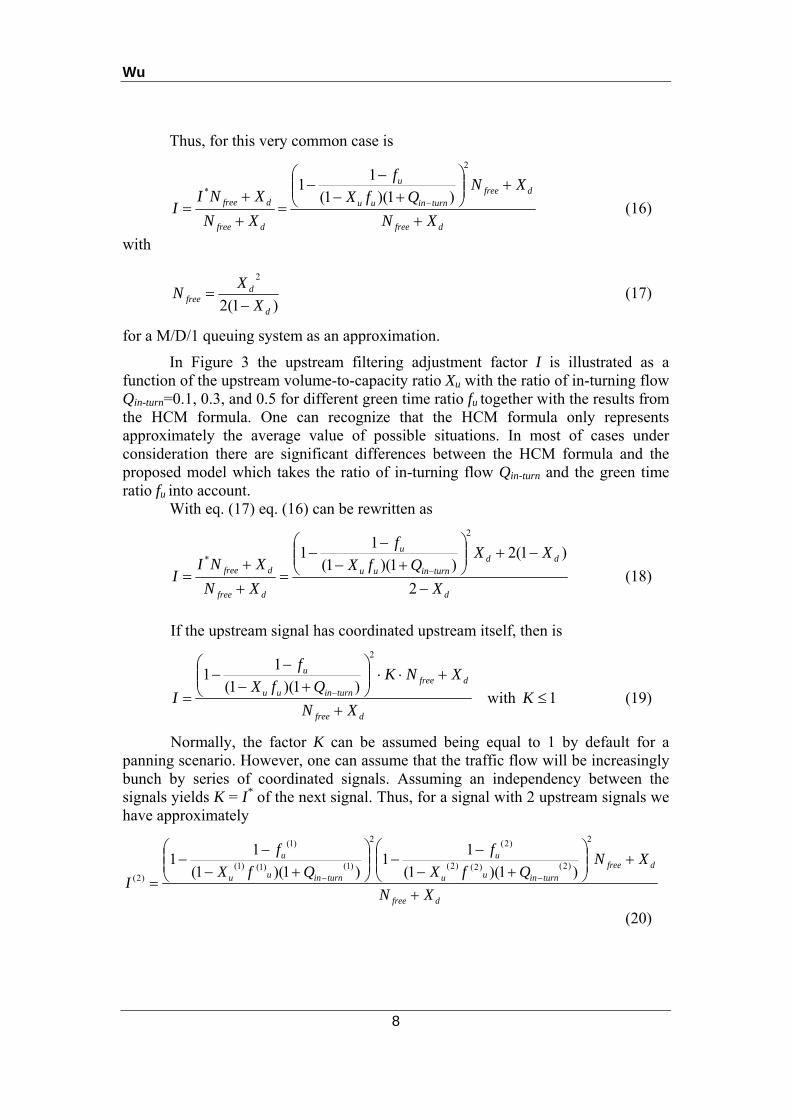
Thus, for this very common case is

dfree

dfreeturninuu

u

dfree

dfree

XN

XNQfX

f

XN

XNII

2

* )1)(1(

11

(16)

with

)1(2

2

d

dfree X

XN

(17)

for a M/D/1 queuing system as an approximation.

In Figure 3 the upstream filtering adjustment factor I is illustrated as a function of the upstream volume-to-capacity ratio Xu with the ratio of in-turning flow Qin-turn=0.1, 0.3, and 0.5 for different green time ratio fu together with the results from the HCM formula. One can recognize that the HCM formula only represents approximately the average value of possible situations. In most of cases under consideration there are significant differences between the HCM formula and the proposed model which takes the ratio of in-turning flow Qin-turn and the green time ratio fu into account.

With eq. (17) eq. (16) can be rewritten as

d

ddturninuu

u

dfree

dfree

X

XXQfX

f

XN

XNII

2

)1(2)1)(1(

11

2

*

(18)

If the upstream signal has coordinated upstream itself, then is

dfree

dfreeturninuu

u

XN

XNKQfX

f

I

2

)1)(1(

11

with 1K (19)

Normally, the factor K can be assumed being equal to 1 by default for a panning scenario. However, one can assume that the traffic flow will be increasingly bunch by series of coordinated signals. Assuming an independency between the signals yields K = I* of the next signal. Thus, for a signal with 2 upstream signals we have approximately

dfree

dfree

turninuu

u

turninuu

u

XN

XNQfX

f

QfX

f

I

2

)2()2()2(

)2(2

)1()1()1(

)1(

)2( )1)(1(

11

)1)(1(

11

(20)

Wu

9

And in general for a signal with m upstream signals is

dfree

dfree

m

jj

turninujj

u

ju

m

XN

XNQfX

f

I

1

2

)()()(

)(

)()1)(1(

11

(21)

Determining Progression Adjustment Factor

According to the methodology in HCM, the progression adjustment factor PF is defined by the equation

Cg

PPF

/1

1

, subject to 0 ≤ PF ≤ 1 (22)

with

C

gRP p (23)

where Rp is the so-called platoon ratio.

The progression adjustment factor PF descript actually the ratio between the delay with steady-state arrivals and the delay with platooned arrivals under the condition of progression.

The platoon ratio Rp is used to describe the quality of signal progression for the corresponding movement group. It is computed as the demand flow rate during the green time divided by the average demand flow rate. HCM (cf. Exhibit 18-8 in HCM2010) provides an indication of the quality of progression associated with selected platoon ratio values (Table 1).

Table 1 - Relationship between Arrival Type and Progression Quality

Platoon Ratio Rp Arrival Type Progression Quality

0.33 1 Very poor

0.67 2 Unfavorable

1.00 3 Random arrivals

1.33 4 Favorable

1.67 5 Highly favorable

2.00 6 Exceptionally favorable

The platoon ratio Rp can be judged from the Table 1 by using the arrival type

designation. Values of arrival type range from 1 to 6. A description of each arrival type is provided in the HCM as following.

Arrival type 1 is characterized by a dense platoon of more than 80 percent of the movement group volume arriving at the start of the red interval.

Wu

10

Arrival type 2 is characterized by a moderately dense platoon arriving in the middle of the red interval or a dispersed platoon containing 40 to 80 percent of the movement group volume arriving throughout the red interval.

Arrival type 3 describes one of two conditions. If the signals bounding the segment are coordinated, then this arrival type is characterized by a platoon containing less than 40 percent of the movement group volume arriving partially during the red interval and partly during the green interval. If the signals are not coordinated, then this arrival type is characterized by platoons arriving at the subject intersection at different points in time over the course of the analysis period such that arrivals are effectively random.

Arrival type 4 is characterized by a moderately dense platoon arriving in the middle of the green interval or a dispersed platoon containing 40 to 80 percent of the movement group volume arriving throughout the green interval. This arrival type is often associated with segments of average length with favorable progression in the subject direction of travel.

Arrival type 5 is characterized by a dense platoon of more than 80 percent of the movement group volume arriving at the start of the green interval.

Arrival type 6 is characterized by a dense platoon of more than 80 percent of the movement group volume arriving at the start of the green interval.

Obviously, the platoon ratio Rp is dependent on the proportion Ppl of vehicles in platoon und on the arriving time of the platoon, ta, within a cycle. HCM doesn’t provide any methodology for calculating the proportion of vehicles in platoon. Fortunately, for the default case in a planning scenario, the proportion Ppl of vehicles in platoon can be given here as (see the previous section, eq.(15))

turninuu

upl QfX

fP

11

)1( (24)

According the description of the arrival types in HCM, the relationship between the platoon ratio as a function of the proportion of vehicles in platoon, Ppl, and the arriving time ta of the platoon can be established. Table 2 shows the values of the platoon ratio according to the HCM description. Unfortunately, the HCM description for the 6 arrival types (T1-T6) does not fill out the whole matrix. The empty cells of the table are filled here with the average values (black bold numbers) calculated from the values in the nearby cells.

Wu

11

Table 2 - Values of platoon ratio Rp according to the HCM description

arriving time of the platoon, ta

Proportion of vehicles in platoon, Ppl

40% 60% 80% 100%

0.0R(1.0G) 1) 1,00 (T3) 0,83 0,33 (T1) 0,00

0.5R 2) 1,00 (T3) 0,67 (T2) 0,92 1,00

1.0R(0.0G) 3) 1,00 (T3) 1,17 1,67 (T5) 2,00 (T6)

0.5G 4) 1,00 (T3) 1,33 (T4) 1,08 1,00

1.0G(0.0R) 5) 1,00 (T3) 0,83 0,33 (T1) 0,00 1) At the beginning of red interval (= at the end of green interval) 2) In the middle of red interval 3) At the beginning of green interval (= at the beginning of green interval) 4) In the middle of green interval 5) At the end of green interval (= at the beginning of red interval), corresponds to 1)

The platoon ratio Rp can also be estimated using the following monograph

(Figure 4). For other Ppl and ta values the platoon ratio Rp can be interpolated using Table 2 or Figure 4.

Figure 4 - Platoon ratio Rp as a function of the proportion of vehicles in platoon, Ppl, and the arriving time of the platoon, ta

Unfortunately, as seen in Figure 8, the curves for the platoon ratio Rp based

on the data in HCM show some stranger shapes and discontinuities. One can question the accuracy of the graph and the values in Table 2. Here, one should take a near look at the derivation. In general, the platoon ratio Rp can be derived by comparing the uniform delay d1 under steady-state arrivals with that under coordinated condition with platoons.

The uniform delay is the delay caused by changing signal phases from green

Wu

12

to red or vice versa. It is only depends on the deterministic arrival patterns and not on the stochastic properties of arrivals. For example, the first term of the Webster’s delay formula gives the uniform delay with a steady-state arrival pattern as follows:

CXCg

Cgd st )/1(2

)/1( 2

,1

(25)

For platooned arrivals the formulation of the uniform delay is more complicated. The uniform delay is in general a function of the degree of saturation X, the green time length g, the cycle tine length C, the ratio of platoon Ppl, the flow rate in the platoon, q2, the flow rate outside of the platoon, q1, the saturation flow rate s. and certainly the arriving time of the platoon, ta (cf. Figure 5). According to the queue development illustrated in Figure 5, a generalized but very comprehensive formulation for the uniform delay d1 can be derived regarding all of those parameters. The derivations can be verified by simulations studies. The formulation is not given here because of the complexity and limited space in the paper. The formulation can be obtained by the author if required.

Figure 5 - Proportion of platoon Ppl and the corresponding queue length for

calculation uniform delay d1

It is always true due to definition:

Cq

DqPpl

2 or

plP

DqCq

2 (26)

where D is the length in time for the platoon.

queue length

q1 s

r g

r g

Ppl

flow

q2

q1

time

time

ta

q2

q1

D

Wu

13

Please note in all formulations for the uniform delay d1 the expression D/C can be replaces by

XC

g

q

sP

q

qP

C

Dplpl

22

(27)

Thus, the parameter D can be totally eliminated from the formulation. The progression adjustment factor PF and the platoon ratio Rp can be

obtained according to the definitions:

std

dPF

,1

1 (28)

and

Cg

CgPFRp /

)/1(1 (29)

The functions of PF and Rp can be normalized to the ratios X, Ppl, g/C, q2/s, and ta/C. That is, we have generally

),,,,( 2

C

t

s

q

C

qPXfPF a

pl and ),,,,( 2

C

t

s

q

C

qPXfR a

plp (30)

In Figure 6 the progression adjustment factor PF and the platoon ratio Rp as functions of ta/C and Ppl with constant values X=0.9, q2/s=0.9, and g/C=0.5 are illustrated. One can recognize clearly the similarity and differences from Figure 6b to Figure 4. A set of monographs were produced for all parameter combinations. These monographs can also be obtained by the author if required.

Wu

14

0

0.2

0.4

0.6

0.8

1

1.2

1.4

1.6

1.8

2

0 0.25 0.5 0.75 1

Progression Adjusm

ent Factor PF [‐]

arriving time of the platoon ta/C [‐]

100%80%60%40%

proportion Ppl of vehicles in platoon

a)

0

0.2

0.4

0.6

0.8

1

1.2

1.4

1.6

1.8

2

0 0.25 0.5 0.75 1

Platoon ratio R

p[‐]


40%

60%

80%

100%

proportion Ppl of vehicles in platoon

b) Figure 6 - PF (a) and Rp (b) as functions of ta/C and Ppl with constant values X=0.9,

q2/s=0.9, and g/C=0.5 For simplifying the formulation of the progression factor PF and platoon ratio

Rp we consider now the case X=1. That is the worst case under consideration regarding delay analyses. This is a significant, but needed simplification in order to get rid of the complicated formulations.

For this special case we have always qC=sg and the uniform delay can be calculated according to the illustration in Figure 5 as following.

For CDta is

Wu

15

CP

C

DqC

gs

C

t

C

D

C

DC

g

q

s

C

D

C

D

Cq

ggs

tDqDCgsDqDq

d

pl

a

a

a

2

2

2

2

22

22

1

2

)()1(

22

)(

2)(

22

(31)

For CDta is

CP

C

DC

D

C

t

C

D

qC

gs

C

DC

D

C

g

q

s

C

D

Cq

DCtDCqggs

DCDqgsDq

d

pl

a

a

b

))1()(1(2

)()1(

22

)(

))()((2

)(22

2

2

2

2

22

22

1

(32)

Please note in both equations the expression D/C can be replaces by

C

g

q

sP

C

Dpl

2

(33)

due to the predefined condition of X=1. Thus, the parameter D can be eliminated. The final expression of the uniform delay for X=1 is,

)max( 1,11 ba ddd (34)

The progression factor is then

std

dPF

,1

1 (35)

with

2|

)/1(2

)/1(1

2

,1

gCC

XCg

Cgd Xst

(36)

And the platoon ratio is

Wu

16

Cg

CgPFRp /

)/1(1 (37)

For an additional simplification we can assume q2=s (normally, it is almost the case in the reality). Thus,

g

D

gs

Dq

Cq

DqPpl

22 and C

gP

C

Dpl (38)

The result of the assumptions X=1 and q2=s is a two-piece linear function for the platoon ratio Rp regarding the ratio ta/C. Rearranging the equations above yields the following final simple equation:

)1(

/

2)1(

//1

2)1(

min

C

t

CgP

C

t

CgPP

Ra

pl

a

plpl

p (39)

The intersection point of the two function branches gives the maximum value of Rp and it indicates the best offset of the platoon with minimized delay. This point can be obtained by setting d1a=d1b. The intersection point is defined by

CgPC

tpl

a /1 (40)

and

plp PR 1max, (41)

The value of Rp depends on the green ratio g/C. Figure 7 shows two examples for g/C=0.5 and g/C=0.6. Comparing Figure 7a with Figure 6b one can recognize, that the pictures (both for g/C=0.5) deliver very similar values for the platoon ratio Rp. That means, the simplifications X=1 and q2/s=1 do not significantly change the values of the platoon ratio Rp.

Wu

17

0

0.2

0.4

0.6

0.8

1

1.2

1.4

1.6

1.8

2

0 0.1 0.2 0.3 0.4 0.5 0.6 0.7 0.8 0.9 1

Platoon ratio R

p[‐]


40%

60%

80%

100%

proportion Ppl of vehicles in platoonproportion Ppl of vehicles in platoon

a)

0

0.2

0.4

0.6

0.8

1

1.2

1.4

1.6

1.8

2

0 0.1 0.2 0.3 0.4 0.5 0.6 0.7 0.8 0.9 1

Platoon ratio R

p[‐]


40%

60%

80%

100%

proportion Ppl of vehicles in platoonproportion Ppl of vehicles in platoon

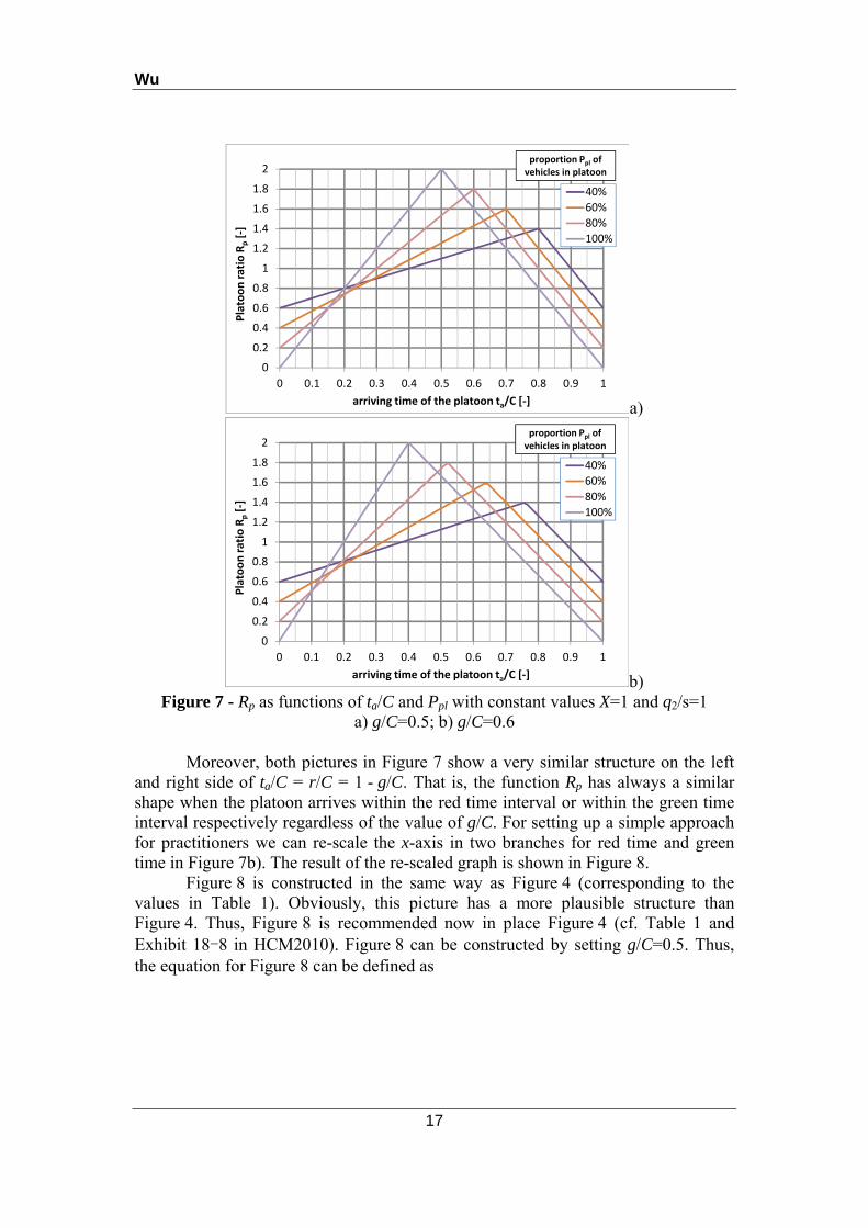
b) Figure 7 - Rp as functions of ta/C and Ppl with constant values X=1 and q2/s=1

a) g/C=0.5; b) g/C=0.6

Moreover, both pictures in Figure 7 show a very similar structure on the left and right side of ta/C = r/C = 1 - g/C. That is, the function Rp has always a similar shape when the platoon arrives within the red time interval or within the green time interval respectively regardless of the value of g/C. For setting up a simple approach for practitioners we can re-scale the x-axis in two branches for red time and green time in Figure 7b). The result of the re-scaled graph is shown in Figure 8.

Figure 8 is constructed in the same way as Figure 4 (corresponding to the values in Table 1). Obviously, this picture has a more plausible structure than Figure 4. Thus, Figure 8 is recommended now in place Figure 4 (cf. Table 1 and Exhibit 18-8 in HCM2010). Figure 8 can be constructed by setting g/C=0.5. Thus, the equation for Figure 8 can be defined as

Wu

18

)1(4)1(

1/2

4)1(

min

C

tP

C

t

PP

Ra

pl

a

plpl

p (42)

The factor ta/C is now defined as the proportion of the green time (G) or the red time (R).

Figure 8 - Simplified graph for estimation the platoon ratio Rp as a function of the proportion of vehicles in platoon Ppl and the arriving time of the platoon ta

CONCLUSIONS

For calculating the progression adjustment factor and the upstream filtering adjustment factor at signalized intersections, two simple models are introduced in order to modify the approaches in HCM. The new models are generalizations of the existing HCM procedures. According to the new models, the upstream filtering adjustment factor is a function of the upstream volume-to-capacity ratio, the upstream green time ratio, and the in-turning volume from the side roads. The progression adjustment factor can be defined by the equation (16). The platoon ratio is a function of the proportion of vehicles in platoon, the green time ratio, and the arriving time of the platoon within the cycle length. The platoon ratio can be defined by the equation (39). With the new models, the delays at coordinated signals can be more accurately estimated for default conditions in planning sceneries.

REFERENCES Akcelik, R. and E. Chung. Calibration of the Bunched Exponential Distribution of

Arrival Headways, In Road and Transport Research, Vol. 3, No. 1, 1994, pp. 42–59.

Akcelik, R. Australian Road Research Report 123: Traffic Signals: Capacity and Timing Analysis, Australian Road Research Board, Kew, Victoria, Australia, 1981.

Wu

19

Berry, D. and P. Gandhi. Headway Approach to Intersection Capacity, In Highway Research Record 453, HRB, National Research Council, Washington, D.C., 1973, pp. 56–60.

Bonneson, J., M. Pratt, and M. Vandehey. Predicting the Performance of Automobile Traffic on Urban Streets: Final Report, NCHRP Project 3‐79, NCHRP, National Research Council, Washington, D.C., January 2008.

Catling, I. A Time ‐ Dependent Approach To Junction Delays, In Traffic Engineering & Control, Vol. 18, No. 11, November 1977, pp. 520–526.Cowan, R. Useful Headway Models, In Transportation Research, Vol. 9, No. 6, Pergamon Press Ltd., 1975, pp. 371–375. Chapter 18/Signalized Intersections Page 18-103 References

Dowling, R., D. Reinke, A. Flannery, P. Ryus, M. Vandehey, T. Petritsch, B. Landis, N. Rouphail, and J. Bonneson. NCHRP Report 616: Multimodal Level of Service Analysis for Urban Streets, TRB, National Research Council, Washington, D.C., 2008.

JHK & Associates. Signalized Intersection Capacity Method, NCHRP Project 3‐28(2), Tucson, Ariz., February 1983.

JHK & Associates. Signalized Intersection Capacity Study: Final Report, NCHRP Project 3‐28(2), Tucson, Ariz., December 1982.

Marshal, W. G. (1974). Some Simple Bounds and Approximations in Queuing. Technical Memorandum Serial T-294. Institute for Management Science and Engineering, The George Washington University, January 1974.

Messer, C. and D. Fambro. Critical Lane Analysis for Intersection Design, In Transportation Research Record 644, TRB, National Research Council, Washington, D.C., 1977, pp. 95–101.

Miller, A. Australian Road Research Bulletin 3: The Capacity of Signalized Intersections in Australia, Australian Road Research Board, Kew, Victoria, Australia, 1968.

Petersen, B. and E. Imre. Swedish Capacity Manual. Stockholm, Sweden, February 1977.

Reilly, W., C. Gardner, and J. Kell. A Technique for Measurement of Delay at Intersections, Report No. FHWA‐RD‐76‐135/137, FHWA, USDOT, Washington, D.C., 1976.

Rouphail, N., J. Hummer, J. Milazzo, and D. Allen. Recommended Procedures for Chapter 9, Signalized Intersections, of the Highway Capacity Manual, Report No. FHWA‐RD‐98‐106, FHWA, USDOT, Washington, D.C., 1999.

Strong, D. and N. Rouphail. Incorporating the Effects of Traffic Signal Progression into the Proposed Incremental Queue Accumulation (IQA) Method, Paper 06‐0107, presented at the TRB 85th Annual Meeting, Washington, D.C., January 2006.

Strong, D., N. Rouphail, and K. Courage. New Calculation Method for Existing and Extended HCM Delay Estimation Procedures, Paper 06‐0106, presented at the TRB 85th Annual Meeting, Washington, D.C., January 2006.

TRB (2000, 2010). Highway Capacity Manual (HCM). Special Report 209. TRB, National Research Council, Washington, D.C.

Wu

20

Webster, F. and B. Cobbe. Traffic Signals, Road Research Technical Paper 56, Her Majesty’s Stationery Office, London, England, 1966.

Wu, N. (1990). Wartezeit und Leistungsfähigkeit von Lichtsignalanlagen unter Berücksichtigung von Instationarität und Teilgebundenheit des Verkehrs (Dissertation). Schriftenreihe des Lehrstuhls für Verkehrswesen der Ruhr-Universität Bochum, Heft 8. Ruhr-Universität Bochum, Bochum, 1990.

Modifying Progression Adjustment Factor and Upstream...

Documents

Transcript of Modifying Progression Adjustment Factor and Upstream...