Modified nonlinear conjugate gradient method with sufficient

RESEARCH Open Access

Modified nonlinear conjugate gradient methodwith sufficient descent condition forunconstrained optimizationJinkui Liu* and Shaoheng Wang

* Correspondence:[email protected] of Mathematics andStatistics, Chongqing Three GorgesUniversity, Chongqing, Wanzhou,People’s Republic of China

Abstract

In this paper, an efficient modified nonlinear conjugate gradient method for solvingunconstrained optimization problems is proposed. An attractive property of themodified method is that the generated direction in each step is always descendingwithout any line search. The global convergence result of the modified method isestablished under the general Wolfe line search condition. Numerical results showthat the modified method is efficient and stationary by comparing with the well-known Polak-Ribiére-Polyak method, CG-DESCENT method and DSP-CG methodusing the unconstrained optimization problems from More and Garbow (ACM TransMath Softw 7, 17-41, 1981), so it can be widely used in scientific computation.Mathematics Subject Classification (2010) 90C26 · 65H10

1 IntroductionThe conjugate gradient method comprises a class of unconstrained optimization algo-

rithms which is characterized by low memory requirements and strong local or global

convergence properties. The purpose of this paper is to study the global convergence

properties and practical computational performance of a modified nonlinear conjugate

gradient method for unconstrained optimization without restarts, and with appropriate

conditions.

In this paper, we consider the unconstrained optimization problem:

min {f (x)|x ∈ Rn}, (1:1)

where f : Rn ® R is a real-valued, continuously differentiable function.

When applied to the nonlinear problem (1.1), a nonlinear conjugate gradient method

generates a sequence {xk}, k ≥ 1, starting from an initial guess x1 Î Rn, using the recur-

rence

xk+1 = xk + αkdk, (1:2)

where the positive step size ak is obtained by some line search, and the search direc-

tion dk is generated by the rule:

dk ={−gk, for k = 1,

−gk + βkdk−1, for k ≥ 2.(1:3)

Liu and Wang Journal of Inequalities and Applications 2011, 2011:57http://www.journalofinequalitiesandapplications.com/content/2011/1/57

© 2011 Liu and Wang; licensee Springer. This is an Open Access article distributed under the terms of the Creative CommonsAttribution License (http://creativecommons.org/licenses/by/2.0), which permits unrestricted use, distribution, and reproduction inany medium, provided the original work is properly cited.

mailto:[email protected]

http://creativecommons.org/licenses/by/2.0

where gk = ▽f (xk) and bk is a scalar. Well-known formulas for bk are called Liu-

Storey (LS) formula, Polak-Ribiére-Polyak (PRP) formula, and are given by

βLSk = − gTk yk−1

gTk−1dk−1(Liu − Storey [1]), (1:4)

βPRPk =

gTk yk−1

‖gk−1‖2 (Polak–Ribiere–Polyak [2, 3]), (1:5)

respectively, where symbol || · || denotes the Euclidean norm and yk-1 = gk - gk-1 .

Their corresponding methods generally specified as LS and PRP conjugate gradient

methods. If f is a strictly convex quadratic function, the both methods are equivalent

in the case that an exact line search is used. If f is non-convex, their behaviors may be

distinctly different. In the past two decades, the convergence properties of LS and PRP

methods have been intensively studied by many researchers (e.g., [1-5]).

In practical computation, the PRP method, which is generally believed to be the most

efficient conjugate gradient methods, and has got meticulous in recent years. One

remarkable property of the method is that they essentially perform a restart if a bad

direction occurs (see [6]). However, Powell [7] constructed an example showed that

the method can cycle infinitely without approaching any stationary point even if an

exact line search is used. This counter-example also indicates that the method has a

drawback that it is impossible to be convergent when the objective function is non-

convex. Therefore, during the past few years, much effort has been investigated to cre-

ate new formulae for bk, which not only possesses global convergence for general func-

tions but also is superior to original method from the computation point of view (see

[8-17]).

In this paper, we further study the conjugate gradient method for the solution of

unconstrained optimization problems. Meanwhile, we focus our attention on the scalar

for bk with [12]. We introduce a version of modified LS conjugate gradient method.

An attractive property of the proposed method is that the generated directions are

always descending. Besides, this property is independent of line search used and the

convexity of objective function. Under the general Wolfe line search condition, we

establish the global convergence of the proposed method. We also do some numerical

experiments by using a large set of unconstrained optimization problems from [18],

which indicates the proposed method possesses better performances when compared

with the classic PRP method, CG-DESCENT method and DSP-CG method. This paper

is organized as follows. In section 2, we propose our algorithm, some assumptions on

objective function and some lemmas. In section 3, global convergence analysis is pro-

vided with the general Wolfe line search condition. In the last section, we perform the

numerical experiments by using a set of large problems, and do some numerical com-

parisons with PRP method, CG-DESCENT method and DSP-CG method.

2 The sufficient descent propertyAlgorithom 2.1:

Step 1: Data x1 Î Rn, ε ≥ 0. Set d1 = -g1, if ||g1|| ≤ ε, then stop.

Step 2: Compute ak by the general Wolfe line searches (s1 Î (δ, 1), s2 ≥ 0):

f (xk + αkdk) ≤ f (xk) + δαkgTk dk, (2:1)


of 12

σ1gTk dk ≤ g(xk + αkdk)Tdk ≤ −σ2g

Tk dk. (2:2)

Step 3: Let xk+1 = xk + ak dk, gk+1 = g(xk+1), if ||gk+1|| ≤ ε, then stop.

Step 4: Generate dk+1 by (1.3) in which bk+1 is computed by

βVLSk+1 = max

{βLSk+1 − u · ||yk||2

(gTk dk)2 · gTk+1dk, 0

},

(u >

14

). (2:3)

Step 5: Set k = k + 1, go to step 2.

In this paper, we prove the global convergence of the new algorithm under the fol-

lowing assumption.

Assumption (H):

(i) The level set Ω = {x Î Rn| f(x) ≤ f(x1)} is bounded, where x1 is the starting point.

(ii) In a neighborhood V of Ω, f is continuously differentiable and its gradient g is

Lipschitz continuous, namely, there exists a constant L >0 such that

||g(x) − g(y)|| ≤ L||x − y||, ∀x, y ∈ V. (2:4)

Obviously, from the Assumption (H) (i), there exists a positive constant ξ, so that

ξ = max {||x − y|| : ∀x, y ∈ �}, (2:5)

where ξ is the diameter of Ω.

From Assumption (H) (ii), we also know that there exists a constant r > 0, such that

||g(x)|| ≤ r, ∀x ∈ V. (2:6)

On some studies of the conjugate gradient methods, the sufficient descent condition

gTk dk ≤ −c||gk||2, c > 0.

plays an important role. Unfortunately, this condition is hard to hold. However, the

following lemma proves the sufficient descent property of Algorithm 2.1 independent

of any line search and the convexity of objective function.

Lemma 2.1 Consider any method (1.2)-(1.3), where βk = βVLSk . We get

gTk dk ≤ −(1 − 1

4u

)||gk||2, ∀k ≥ 1. (2:7)

Proof. Multiplying (1.3) by gTk , we have

gTk dk = −||gk||2 + βkgTk dk−1. (2:8)

From (2.3), if bk = 0, then

gTk dk = −||gk||2 ≤ −(1 − 1

4u

)||gk||2.

If βk = βLSk − u · ||yk−1||2

(gTk−1dk−1)2 · gTk dk−1, then from (1.4) and (2.8), we have

gTk dk = −||gk||2 +(

− gTk yk−1

gTk−1dk−1− u · ||yk−1||2

(gTk−1dk−1)2 · gTk dk−1

)· gTk dk−1

=−gTk yk−1 · gTk−1dk−1 · gTk dk−1 − u||yk−1||2 · (gTk dk−1)

2 − ||gk||2 · (gTk−1dk−1)2

(gTk−1dk−1)2 .

(2:9)


of 12

We apply the inequality

ATB ≤ 12(||A||2 + ||B||2)

to the first term in (2.9) with

AT =(−gk−1dk−1)√

2ugTk , B =

√2u(gTk dk−1)yk−1,

then we have

−gTk yk−1 · gTk−1dk−1 · gTk dk−1 = ATB ≤ (−gTk−1dk−1)2

4u||gk||2 + u (gTk dk−1)2 ||yk−1||2.

From the above inequality and (2.9), we have

gTk dk ≤ −(1 − 1

4u

)||gk||2.

From the above proof, we obtain that the conclusion (2.7) holds.

□

3 Global convergence of the modified methodThe conclusion of the following lemma, often called the Zoutendijk condition, is used

to prove the global convergence of nonlinear conjugate gradient methods. It was ori-

ginally given by Zoutendijk [19] under the Wolfe line searches. In the following

lemma, we will prove the Zoutendijk condition under the general Wolfe line searches.

Lemma 3.1 Suppose Assumption (H) holds. Consider iteration of the form (1.2)-

(1.3), where dk satisfies gTk dk < 0 for k Î N + and ak satisfies the general Wolfe line

searches. Then

∑k≥1

(gTk dk)2

||dk||2 < +∞. (3:1)

Proof. From (2.2) and Assumption (H) (ii), we have

− (1 − σ1)dTk gk ≤ dTk (gk+1 − gk) ≤ ||dk|| · ||gk+1 − gk|| ≤ Lαk||dk||,

then

αk ≥ σ1 − 1L

· dTk gk||dk||2 .

From (2.1) and the equality above, we get

f (xk) − f (xk + αkdk) ≥ δ(1 − σ1)L

· (dTk gk)2

||dk||2 .

From Assumption (H) (i), and combining this inequality, we have

∑k≥1

(gTk dk)2

||dk||2 < +∞.

□


of 12

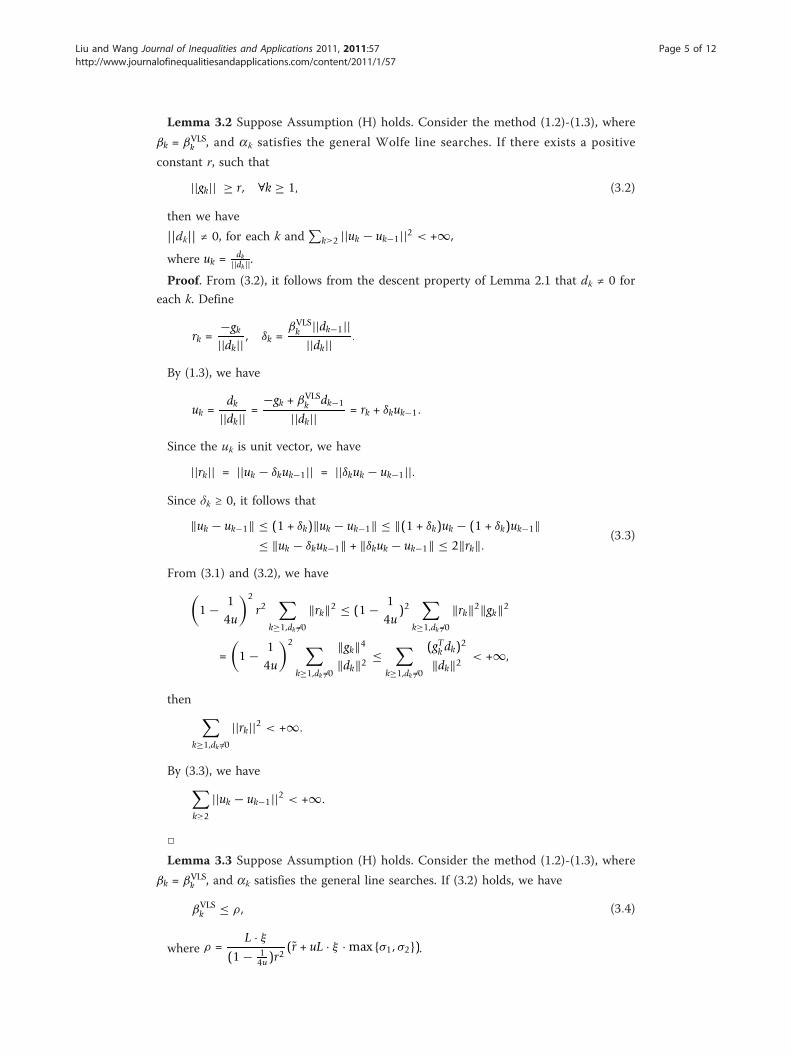
Lemma 3.2 Suppose Assumption (H) holds. Consider the method (1.2)-(1.3), where

βk = βVLSk , and ak satisfies the general Wolfe line searches. If there exists a positive

constant r, such that

||gk|| ≥ r, ∀k ≥ 1, (3:2)

then we have

||dk|| ≠ 0, for each k and∑

k≥2 ||uk − uk−1||2 < +∞,

where uk =dk

||dk||.

Proof. From (3.2), it follows from the descent property of Lemma 2.1 that dk ≠ 0 for

each k. Define

rk =−gk||dk|| , δk =

βVLSk ||dk−1||

||dk|| .

By (1.3), we have

uk =dk

||dk|| =−gk + βVLS

k dk−1

||dk|| = rk + δkuk−1.

Since the uk is unit vector, we have

||rk|| = ||uk − δkuk−1|| = ||δkuk − uk−1||.

Since δk ≥ 0, it follows that

‖uk − uk−1‖ ≤ (1 + δk)‖uk − uk−1‖ ≤ ‖(1 + δk)uk − (1 + δk)uk−1‖≤ ‖uk − δkuk−1‖ + ‖δkuk − uk−1‖ ≤ 2‖rk‖.

(3:3)

From (3.1) and (3.2), we have(1 − 1

4u

)2

r2∑

k≥1,dk =0‖rk‖2 ≤ (1 − 1

4u)2

∑k≥1,dk =0

‖rk‖2‖gk‖2

=(1 − 1

4u

)2 ∑k≥1,dk =0

‖gk‖4‖dk‖2 ≤

∑k≥1,dk =0

(gTk dk)2

‖dk‖2 < +∞,

then ∑k≥1,dk =0

||rk||2 < +∞.

By (3.3), we have∑k≥2

||uk − uk−1||2 < +∞.

□Lemma 3.3 Suppose Assumption (H) holds. Consider the method (1.2)-(1.3), where

βk = βVLSk , and ak satisfies the general line searches. If (3.2) holds, we have

βVLSk ≤ ρ, (3:4)

where ρ =L · ξ

(1 − 14u)r

2(r + uL · ξ · max {σ1, σ2}).


of 12

Proof. Define sk-1 = xk - xk-1. From (2.2), we have

|gTk dk−1||gTk−1dk−1|

≤ max {σ1, σ2}. (3:5)

By (1.4), (2.3), (2.4)-(2.7) and (3.5), we have

|βVLSk | = |βLS

k − u · ||yk−1||2(gTk−1dk−1)

2 · gTk dk−1| ≤ |βLSk | + u · ||yk−1||2

(gTk−1dk−1)2 · |gTk dk−1|

≤ ||gk − gk−1|||gTk−1dk−1|

( ||gk|| + u · ||gk − gk−1|||gTk−1dk−1|

· |gTk dk−1| )

≤ L · ||xk − xk−1||(1 − 1

4u )||gk−1||2

(r + u · L · ||xk − xk−1|| · |gTk dk−1|

|gTk−1dk−1|

)

≤ L · ||sk−1||(1 − 1

4u )r2(r + u · L · ||sk−1|| · max {σ1, σ2})

≤ L · ξ(1 − 1

4u )r2(r + uL · ξ · max {σ1, σ2}) = ρ.

□Theorem 3.1 Suppose Assumption (H) holds. Consider the method (1.2)-(1.3), where

βk = βVLSk and ak satisfies the general line searches, then either gk = 0 for some k or

lim infk→+∞

||gk|| = 0.

Proof. If gk = 0 for some k, we have the conclusion. In the following, we suppose

that gk ≠ 0 for all k, then (3.2) holds, and we can obtain a contradiction.

We also define ui =di

||di||, then for any l, k Î Z +, and l > k, we have

xl − xk−1 =l∑

i=k

|| xi − xi−1|| · ui−1 =l∑

i=k

|| si−1|| · uk−1 +l∑

i=k

|| si−1|| · (ui−1 − uk−1).

By the triangle inequality, we have

l∑i=k

|| si−1|| ≤ ||xl−xk−1||+l∑

i=k

|| si−1||· ||ui−1−uk−1|| ≤ ξ+l∑

i=k

|| si−1||· ||ui−1−uk−1||. (3:6)

Let Δ be a positive integer, chosen large enough that

≥ 4ρ, (3:7)

where ξ and r appear in Lemma 3.3.

Since the conclusion of Lemma 3.2, there exits a k0 large enough such that

∑i≥k0

||ui − ui−1||2 <14

. (3:8)

If ∀i Î [k + 1, k + Δ], then by (3.7) and the Cauchy-Schwarz inequality, we have

||ui−1−uk−1|| ≤i−1∑j=k

||uj − uj−1|| ≤ (i − k)12

⎛⎝ i−1∑

j=k

||uj − uj−1||2⎞⎠

12

≤ 12 ·

(14

)12=12.


of 12

Combining this inequality and (3.6), we have

l∑i=k

||si−1|| ≤ ξ +12

l∑i=k

||si−1|| ,

then

l∑i=k

||si−1|| < 2ξ . (3:9)

when ∀l Î [k + 1, k + Δ].

Define λ = L

(1− 14u )r

2(r + uL · max {σ1, σ2}). From Lemma 3.3, we have

βVLSk ≤ λ||sk−1 ||.

Define Si = 2l2 ||si||2. By (1.3) and (2.6), for ∀l ≥ k0 + 1, we have

||dl||2 = || − gl + βl · dl−1||2 ≤ 2||gl ||2 + 2β2l ||dl−1||2

≤ 2r2 + 2λ2||sl−1||2||dl−1||2 ≤ 2r2 + Sl−1||dl−1||2.From the inequality above, we have

||dl||2 ≤ 2r2

⎛⎝ l∑

i=k0+1

l−1∏j=i

Sj

⎞⎠ + ||dk0 ||2

l−1∏j=i

Sj. (3:10)

By the inequality above, the product is defined to be one whenever the index range is

vacuous. Let us consider a product of Δ consecutive Si, where k ≥ k0. Combining (2.5),

(3.7) and (3.9), by the arithmetic-geometric mean inequality, we have

k+−1∏j=k

Sj =k+−1∏j=k

2λ2||si||2 =

⎛⎝k+−1∏

j=k

√2λ||si||

⎞⎠

2

≤(∑k+−1

j=k

√2λ||si||

)2

≤(2√2λξ

)2

≤(2√2ρ

)2

≤ 12

,

then the sum in (3.10) is bounded, independent of l.

From Lemma 3.2 and (3.2), we have

(1 − 1

4u

)2

r4∑

k≥1,dk =0

1||dk||2 ≤

(1 − 1

4u

)2 ∑k≥1,dk =0

||gk||4||dk||2 ≤

∑k≥1,dk =0

(gTk dk)2

||dk||2 < +∞,

which contradicts the result of the Theorem 3.1 that the bound for ||dl||, indepen-

dent of l > k0. Hence,

lim infk→+∞

||gk|| = 0.

□

4 Numerical resultsIn this section, we compare the modified conjugate gradient method, denoted VLS

method, to the PRP method, CG-DESCENT (h = 0.01) method [12] and DSP-CG (C =


of 12

0.5) method [17] in the average performance and the CPU time performance under the

general Wolfe line search where δ = 0.01, s1 = s2 = 0.1 and u = 0.5. The tested 78

problems come from [18], and the termination condition of the experiments is ||gk|| ≤

10-6, or It-max >9999 where It-max denotes the maximal number of iterations. All

codes were written in Mat lab 7.0 and run on a PC with 2.0 GHz CPU processor and

512 MB memory and Windows XP operation system.

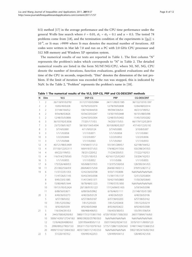
The numerical results of our tests are reported in Table 1. The first column “N”

represents the problem’s index which corresponds to “N” in Table 2. The detailed

numerical results are listed in the form NI/NF/NG/CPU, where NI, NF, NG, CPU

denote the number of iterations, function evaluations, gradient evaluations and the

time of the CPU in seconds, respectively. “Dim” denotes the dimension of the test pro-

blem. If the limit of iteration was exceeded the run was stopped, this is indicated by

NaN. In the Table 2, “Problem” represents the problem’s name in [18].

Table 1 The numerical results of the VLS, DSP-CG, PRP and CG-DESCENT methods

N Dim VLS DSP-CG PRP CG-DESCENT

1 2 26/118/97/0.0792 31/127/103/0.0984 24/111/85/0.1585 36/132/107/0.1397

2 2 10/65/49/0.028 10/70/55/0.0374 12/78/59/0.0698 12/64/48/0.0314

3 2 37/184/164/0.2 138/743/644/0.8 99/394/336/0.4 40/213/189/0.2

4 2 9/54/46/0.0626 10/34/23/0.0247 13/30/19/0.0448 16/101/88/0.098

5 2 12/48/35/0.0806 12/44/33/0.0304 12/48/35/0.0402 11/45/33/0.0282

6 3 36/107/92/0.3036 77/201/171/0.5 74/203/175/0.5 66/179/152/0.2819

7 3 23/72/58/0.1827 58/183/154/0.4594 30/100/80/0.2027 47/143/122/0.192

8 3 3/7/4/0.0081 4/11/9/0.0124 3/7/4/0.0085 3/10/8/0.007

9 3 1/1/1/0.0058 1/1/1/0.0071 1/1/1/0.0058 1/1/1/0.0061

10 3 1/2/2/0.0044 1/2/2/0.0057 1/2/2/0.0052 1/2/2/0.0036

11 3 1/1/1/0.0568 1/1/1/0.0563 1/1/1/0.0561 1/1/1/0.0553

12 4 40/121/98/0.3409 174/584/511/1.0 101/341/289/0.7 62/198/164/0.2

13 4 37/150/122/0.3111 169/419/371/0.5 174/482/417/0.6 103/298/247/0.5

14 4 69/225/199/0.5 78/251/220/0.2 71/234/203/0.3 77/222/192/0.3

15 4 116/314/270/0.65 71/231/185/0.3 42/161/125/0.2451 53/204/162/0.3

16 5 1/1/1/0.0055 1/1/1/0.0052 1/1/1/0.006 1/1/1/0.0055

17 6 175/526/469/0.5 165/608/537/0.5 113/375/330/0.8 128/395/341/0.5

18 11 251/602/556/0.9 260/640/575/0.8 264/667/603/1.5 379/915/827/1.2

19 6 11/37/22/0.1353 12/42/26/0.0708 9/33/17/0.0696 NaN/NaN/NaN/NaN

7 11/47/26/0.1143 10/43/24/0.0598 11/39/17/0.1137 12/51/32/0.0834

8 9/45/23/0.1085 11/47/24/0.1371 10/42/19/0.0883 11/50/26/0.0643

9 15/80/48/0.1644 18/78/48/0.1223 17/90/57/0.1850 NaN/NaN/NaN/NaN

10 19/131/95/0.2424 20/138/97/0.1221 17/124/84/0.1435 5/59/34/0.0398

11 6/88/56/0.0671 6/89/56/0.0962 6/76/46/0.1111 21/148/105/0.1383

20 3 4/40/26/0.0273 4/40/26/0.0129 4/40/26/0.029 4/40/26/0.0106

5 6/57/38/0.032 6/57/38/0.0187 6/57/38/0.0203 6/57/38/0.0162

10 7/81/52/0.0362 7/81/52/0.025 7/81/52/0.0458 7/81/52/0.0219

15 8/92/60/0.039 8/92/60/0.0468 8/92/60/0.0622 8/92/60/0.0308

21 5 116/334/291/0.3 168/468/406/0.5 156/433/383/0.5 135/391/336/0.4

8 2443/7083/6293/8.0 5883/17312/15381/19.0 6720/19530/17300/20.0 2607/7589/6716/8.0

10 5009/14293/12724/18.0 9890/29020/25790/30.0 NaN/NaN/NaN/NaN NaN/NaN/NaN/NaN

12 1576/4629/4080/6.0 3297/9564/8505/11.0 3507/10432/9234/13.0 3370/10111/8930/12.0

15 2990/8952/7903/13.0 3953/11755/10379/16.0 5775/17288/15329/24.0 5749/17442/15368/25.0

20 4909/15142/13464/26.0 4655/13601/12145/23.0 NaN/NaN/NaN/NaN 5902/18524/16282/34.0

22 5 57/220/187/0.2 109/495/422/0.3 129/499/434/1.0 128/485/421/0.8


of 12

Firstly, in order to rank the average performance of all above conjugate gradient

methods, one can compute the total number of function and gradient evaluation by

the formula

Ntota1 = NF + l ∗ NG, (4:1)

Table 1 The numerical results of the VLS, DSP-CG, PRP and CG-DESCENT methods(Continued)

10 116/506/434/0.5 207/883/768/0.6 90/379/328/0.3 147/571/486/0.4

15 131/570/499/0.5 245/1100/969/0.7 434/1467/1298/2.2 663/2262/1996/2.0

20 241/922/814/0.8 447/1740/1520/2.1 941/2959/2612/3.0 734/2452/2181/2.0

30 185/826/732/0.7 1218/3775/3414/4.0 771/2531/2193/3.0 810/2438/2264/3.0

50 471/1466/1295/1.8 1347/4048/3637/4.0 952/2788/2511/3.0 744/2342/2056/3.0

23 5 30/136/113/0.1086 36/230/185/0.2 32/151/124/0.3752 39/174/141/0.2371

10 77/396/341/0.9 105/623/510/0.6 90/383/324/0.8 94/404/345/0.6

50 67/340/277/0.8 79/470/382/0.5 64/344/280/0.5 81/375/313/0.3

100 30/176/138/0.2486 29/206/158/0.2494 23/160/122/0.2212 31/184/141/0.2361

200 27/171/126/0.4232 29/226/170/0.5 21/174/128/0.4081 25/171/126/0.4088

300 27/187/138/0.9818 23/194/144/0.9981 28/192/143/1.0207 26/186/139/1.0293

24 50 44/95/87/0.1996 42/92/90/0.2505 45/93/85/0.3426 43/95/90/0.2616

100 55/128/118/0.3252 62/138/131/0.3716 58/120/113/0.4573 53/116/108/0.3238

200 62/132/126/2.0277 57/133/128/2.0188 64/135/128/2.0248 59/123/118/1.7219

500 54/112/110/91.2260 53/115/108/104.8456 59/127/116/101.6207 51/110/105/89.7073

25 100 26/118/97/0.1037 31/127/103/0.1672 24/111/85/0.2798 36/124/99/0.1204

200 27/120/98/0.3045 31/127/103/0.1881 24/111/85/0.2808 34/125/102/0.1533

500 27/120/98/0.6795 31/127/103/0.6758 24/111/85/0.6181 31/129/106/0.8847

1000 27/120/98/2.3859 31/127/103/2.4379 24/111/85/2.1821 37/142/116/3.5741

1500 27/120/98/5.3518 32/129/104/5.5164 24/111/85/4.7644 34/132/106/7.2731

2000 27/120/98/9.6130 32/129/104/10.0272 24/111/85/8.8878 32/128/103/12.8140

26 100 58/176/148/0.6985 161/521/456/0.5 169/562/483/0.6 77/227/187/0.5

200 58/176/148/0.2648 188/641/554/0.8 199/676/576/1.4 54/172/141/0.3289

500 58/176/148/1.0814 109/373/322/2.1 129/431/367/2.5 69/215/180/1.6

1000 58/176/148/3.6623 123/412/349/8.3 229/788/675/16.9 101/322/271/8.7

1500 58/176/148/8.05 199/672/578/30.1 100/329/280/16.0 66/210/174/12.4

2000 58/176/148/14.5905 189/650/572/98.3 128/428/363/36.0 69/210/173/22.9

27 500 2610/3823/3822/34.0 5231/7301/7300/66.0 1842/3236/3235/26.0 1635/2926/2925/34.0

1000 299/347/346/9.9 446/524/523/14.1 133/232/231/6.2 247/418/417/16.9

1500 18/30/29/1.7112 16/26/25/1.4134 19/36/35/2.0484 18/38/37/2.9408

2000 2/6/5/0.5139 2/6/5/0.5119 2/6/5/0.5156 2/6/5/0.6810

28 100 5/11/6/0.0715 6/13/7/0.0800 7/15/8/0.0958 7/15/8/0.0966

200 6/13/7/0.2986 7/15/8/0.3452 7/15/8/0.3440 7/15/8/0.3469

500 6/13/7/1.8647 7/15/8/2.1275 7/15/8/2.1656 7/15/8/2.1700

1000 6/13/7/7.3738 7/15/8/8.4909 7/15/8/8.7004 7/15/8/8.6138

1500 6/13/7/16.5460 7/15/8/19.0531 7/15/8/19.3655 7/15/8/19.3503

2000 6/13/7/29.5658 7/15/8/33.8840 7/15/8/34.7553 7/15/8/34.5185

29 100 35/81/75/0.4161 34/79/73/0.2022 35/81/75/0.3982 33/77/70/0.1995

200 34/77/73/0.3871 35/79/73/0.2124 33/75/71/0.3758 31/70/58/0.1880

500 35/78/73/0.5172 34/76/71/0.4660 35/78/74/0.5094 34/76/71/0.6669

1000 36/81/77/1.7980 36/81/77/1.7444 34/76/72/1.6832 36/81/77/2.4956

1500 37/86/81/4.2266 36/84/79/3.9720 37/86/81/4.1950 36/84/79/5.6613

2000 37/86/80/7.5140 36/83/76/7.0520 37/86/80/7.5255 35/80/73/9.7701


of 12

where l is some integer. According to the results on automatic differentiation [20,21],

the value of l can be set to 5, i.e.

Ntota1 = NF + 5 ∗ NG. (4:2)

That is to say, one gradient evaluation is equivalent to five function evaluations if

automatic differentiation is used.

By making used of (4.2), we compare the VLS method with DSP-CG method, PRP

method and CG-DESCENT method as follows: for the ith problem, compute the total

numbers of function evaluations and gradient evaluations required by the VLS method,

DSP-CG method, PRP method and CG-DESCENT method by formula (4.2), and

denote them by Ntotal,i (VLS), Ntotal,i (DSP-CG), Ntotal,i (PRP) and Ntotal,i (CG-DES-

CENT), respectively. Then we calculate the ratio

γi(DSP - CG) =Ntotal,i(DSP - CG)

Ntotal,i(VLS),

γi(PRP) =Ntotal,i(PRP)Ntotal,i(VLS)

,

γi(CG - DESCENT) =Ntotal,i(CG - DESCENT)

Ntotal,i(VLS).

If the i0th problem is not run by the method, we use a constant l = max{gi(method)|i Î S1} instead of γi0 (the method), where S1 denotes the set of the test pro-

blems which can be run by the method. The geometric mean of these ratios for VLS

method over all the test problems is defined by

γ (DSP - CG) =

(∏i∈S

γi(DSP - CG)

) 1|S|

,

γ (PRP) =

(∏i∈S

γi(PRP)

) 1|S|

,

γ (CG - DESCENT) =

(∏i∈S

γi(CG - DESCENT)

) 1|S|

,

where S denotes the set of the test problems, and |S| denotes the number of ele-

ments in S. One advantage of the above rule is that, the comparison is relative and

hence does not be dominated by a few problems for which the method requires a

great deal of function evaluations and gradient functions.

Table 2 The list of the tested problems

N Problem N Problem N Problem N Problem N Problem

1 ROSE 7 BRAD 13 WOOD 19 JNSAM 25 ROSEX

2 FROTH 8 GAUSS 14 KOWOSB 20 VAEDIM 26 SINGX

3 BADSCP 9 MEYER 15 BD 21 WATSON 27 BV

4 BADSCB 10 GULF 16 OSB1 22 PEN2 28 IE

5 BEALE 11 BOX 17 BIGGS 23 PEN1 29 TRID

6 HELIX 12 SING 18 OSB2 24 TRIG


of 12

According to the above rule, it is clear that g (VLS) = 1. The values of g (DSP-CG), g(PRP) and g (CG-DESCENT) are listed in Table 3.

Secondly, we adopt the performance profiles by Dolan and Moré [22] to compare the

VLS method to the DSP-CG method, PRP method and CG-DESCENT method in the

CPU time performance (see Figure 1) In Figure 1,

X = τ , Y = P{log2(rp,s) ≤ τ : 1 ≤ s ≤ ns}.

That is, for each method, we plot the fraction P of problems for which the method is

within a factor τ of the best time. The left side of the figure gives the percentage of the

test problems for which a method is fastest; the right side gives the percentage of the

test problems that were successfully solved by each of the methods. The top curve is

the method that solved the most problems in a time that was within a factor τ of the

best time. Since the top curve in Figure 1 corresponds to VLS method, this method is

clearly fastest for this set for 78 test problems. In particular, the VLS method is fastest

for about 60% of the test problems, and it ultimately solves 100% of the test problems.

From Table 3 and Figure 1, it is clear that the VLS method performs better in the

average performance and the CPU time performance, which implies that the proposed

modified method is computationally efficient.

Table 3 Relative efficiency of the VLS, DSP-CG, PRP and CG-DESCENT methods

VLS DSP-CG PRP CG-DESCENT

1 1.2275 1.2177 1.2186

0 2 4 6 8 100

0.1

0.2

0.3

0.4

0.5

0.6

0.7

0.8

0.9

1

X

Y

VLS methodDSP−CG methodPRP methodCG−DESCENT method

Figure 1 Performance profiles of the conjugate gradient methods with respect to CPU time.


of 12

AcknowledgementsThe authors wish to express their heart felt thanks to the referees and Professor K. Teo for their detailed and helpfulsuggestions for revising the manuscript. At the same time, we are grateful for the suggestions of Lijuan Zhang. Thiswork was supported by The Nature Science Foundation of Chongqing Education Committee (KJ091104, KJ101108)and Chongqing Three Gorges University (09ZZ-060).

Authors’ contributionsJinkui Liu carried out the new method studies, designed all the steps of proof in this research and drafted themanuscript. Shaoheng Wang participated in writing the all codes of the algorithm and suggested many good ideasthat made this paper possible. All authors read and approved the final manuscript.

Competing interestsThe authors declare that they have no competing interests.

Received: 3 March 2011 Accepted: 17 September 2011 Published: 17 September 2011

References1. Liu, Y, Storey, C: Efficient generalized conjugate gradient algorithms. Part 1: theory. J Optim Theory Appl. 69, 129–137 (1992)2. Polak, E, Ribire, G: Note sur la convergence de directions conjugees. Rev Francaise Informat Recherche Operatinelle 3e

Annee. 16, 35–43 (1969)3. Polak, BT: The conjugate gradient method in extreme problems. USSR Comput Math Math Phys. 9, 94–112 (1969).

doi:10.1016/0041-5553(69)90035-44. Gaohang, Yu, Yanlin, Zhao, Zengxin, Wei: A descent nonlinear conjugate gradient method for large-scale unconstrained

optimization. Appl Math Comput. 187, 636–643 (2007). doi:10.1016/j.amc.2006.08.0875. Jinkui, Liu, Xianglin, Du, Kairong, Wang: Convergence of descent methods with variable parameters. Acta Math Appl Sin

33, 222–230 (2010). (in Chinese)6. Hager, WW, Zhang, H: A survey of nonlinear conjugate gradient methods. Pac J Optim. 2, 35–58 (2006)7. Powell, MJD: Nonconvex minimization calculations and the conjugate gradient method. In Numerical Analysis (Dundee,

1983). Lecture Notes in Mathematics, vol. 1066, pp. 122–141.Springer, Berlin (1984)8. Andrei, N: Scaled conjugate gradient algorithms for unconstrained optimization. Comput Optim Appl. 38, 401–416

(2007). doi:10.1007/s10589-007-9055-79. Andrei, N: Another nonlinear conjugate gradient algorithm for unconstrained optimization. Optim Methods Softw. 24,

89–104 (2009). doi:10.1080/1055678080239332610. Birgin, EG, Martínez, JM: A spectral conjugate gradient method for unconstrained optimization. Appl Math Optim. 43,

117–128 (2001). doi:10.1007/s00245-001-0003-011. Dai, Y-H, Liao, L-Z: New conjugacy conditions and related nonlinear conjugate gradient methods. Appl Math Optim. 43,

87–101 (2001). doi:10.1007/s00245001001912. Hager, WW, Zhang, H: A new conjugate gradient method with guaranteed descent and an efficient line search. SIAM J

Optim. 16, 170–192 (2005). doi:10.1137/03060188013. Li, G, Tang, C, Wei, Z: New conjugacy condition and related new conjugate gradient methods for unconstrained

optimization. J Comput Appl Math. 202, 523–539 (2007). doi:10.1016/j.cam.2006.03.00514. Wei, Z, Li, G, Qi, L: New quasi-Newton methods for unconstrained optimization problems. Appl Math Comput. 175,

1156–1188 (2006). doi:10.1016/j.amc.2005.08.02715. Zhang, L, Zhou, W, Li, D-H: A descent modified Polak-Ribiére-Polyak conjugate gradient method and its global

convergence. IMA J Numer Anal. 26, 629–640 (2006). doi:10.1093/imanum/drl01616. Yuan, G: modified nonlinear conjugate gradient method with sufficient descent property for large-scale optimization

problems. Optim Lett. 3, 11–21 (2009). doi:10.1007/s11590-008-0086-517. Gaohang, Yu, Lutai, Guan, Wufan, Chen: Spectral conjugate gradient methods with sufficient descent property for large-

scale unconstrained optimization. Optim Methods Softw. 23, 275–293 (2008). doi:10.1080/1055678070166134418. More, JJ, Garbow, BS, Hillstrome, KE: Testing unconstrained optimization software. ACM Trans Math Softw. 7, 17–41

(1981). doi:10.1145/355934.35593619. Zoutendijk, G: Nonlinear programming, computational methods. In: Abadie J (ed.) Integer and Nonlinear Programming.

pp. 37–86. North-Holland, Amsterdam (1970)20. Dai, Y, Ni, Q: Testing different conjugate gradient methods for large-scale unconstrained optimization. J Comput Math.

213, 11–320 (2003)21. Griewank, A: On automatic differentiation. In: Iri M, Tannabe K (eds.) Mathematical Programming: Recent Developments

and Applications. pp. 84–108. Kluwer Academic Publishers, Dordrecht (1989)22. Dolan, ED, Moré, JJ: Benchmarking optimization software with performance profiles. Math Program. 91, 201–213 (2001)

doi:10.1186/1029-242X-2011-57Cite this article as: Liu and Wang: Modified nonlinear conjugate gradient method with sufficient descentcondition for unconstrained optimization. Journal of Inequalities and Applications 2011 2011:57.


of 12

Modified nonlinear conjugate gradient method with sufficient

Documents

Transcript of Modified nonlinear conjugate gradient method with sufficient