Modern Spatial Econometrics in Practice: A Guide to...
43
Modern Spatial Econometrics in Practice: A Guide to GeoDa, GeoDaSpace and PySAL Luc Anselin Sergio J. Rey November 10, 2014 DRAFT – Do Not Quote Copyright © 2014 Luc Anselin and Sergio J. Rey, All Rights Reserved
Transcript of Modern Spatial Econometrics in Practice: A Guide to...

Modern Spatial Econometrics in Practice:
A Guide to GeoDa, GeoDaSpace and PySAL
Luc Anselin Sergio J. Rey
November 10, 2014
DRAFT – Do Not Quote
Copyright © 2014 Luc Anselin and Sergio J. Rey, All Rights
Reserved

Chapter 3
Spatial Weights:Contiguity
Spatial weights are a key component in any cross-sectional analysis ofspatial dependence. They are an essential element in the specificationof the spatial variables in a model, such as the spatially lagged depen-dent variable and spatially lagged explanatory variables, as shown inEquations 1.1 and 1.2 for the spatial lag and spatial error model.
Formally, the weights express the neighbor structure between theobservations as a n × n matrix W in which the elements wij of thematrix are the spatial weights:
W =���������
w11 w12 . . . w1n
w21 w22 . . . w2n⋮ ⋮ � ⋮wn1 wn2 . . . wnn
���������.
The spatial weights wij are non-zero when i and j are neighbors, andzero otherwise. By convention, the self-neighbor relation is excluded,so that the diagonal elements of W are zero, wii = 0.
In its most simple form, the spatial weights matrix expresses theexistence of a neighbor relation in binary form, with weights 1 and 0.Formally, each spatial unit is represented in the matrix by a row i, andthe potential neighbors by the columns j, with j ≠ i. The existenceof a neighbor relation between the spatial unit corresponding to row iand the one matching column j follows then as wij =Wi,j = 1.
There are many criteria on which the construction of the spatialweights can be based. A comprehensive discussion is beyond the cur-rent scope. We focus on the two most common operational approachesand distinguish between a neighborhood relation based on the notionof contiguity and one derived from distance measures. Intrinsically,
39

40 CHAPTER 3. SPATIAL WEIGHTS: CONTIGUITY
contiguity is most appropriate for geographic data expressed as poly-gons (so-called areal units), whereas distance is suited for point data,although in practice the distinction is not that absolute. In fact, poly-gon data can be represented by their centroid or central point, whichthen lends itself to the computation of distance. Similarly, a tessel-lation can be constructed for point data (e.g., Thiessen polygons),which allows for the determination of contiguity relationships betweenthe polygons in the tesselation.
In this Chapter, we restrict our attention to contiguity weights. Wefirst define some basic concepts and then proceed with a descriptionof the weights functionality in each of GeoDa, GeoDaSpace and PySAL.Distance-based weights are covered in Chapter 4.
3.1 Basic Principles
3.1.1 Rook and Queen Contiguity
Contiguity means that two spatial units share a common border ofnon-zero length. Operationally, we can further distinguish betweena rook and a queen criterion of contiguity, in analogy to the movesallowed for the such-named pieces on a chess board. The rook criteriondefines neighbors by the existence of a common edge between twospatial units. The queen criterion is somewhat more encompassingand defines neighbors as spatial units sharing a common edge or acommon vertex.1 Therefore, the number of neighbors according to thequeen criterion will always be at least as large as for the rook criterion.
In practice, the construction of the spatial weights from the ge-ometry of the data cannot be done by visual inspection or manualcalculation, except in the most trivial of situations. To assess whethertwo polygons are contiguous requires the use of explicit spatial datastructures to deal with the location and arrangement of the polygons.
The way in which contiguity between polygons can be assessed ina GIS depends on its internal representation of the geometric features.The easiest situation is when the data representation in the GIS al-ready captures topology, e.g., by using a node-arc-area approach ora connected edge list to store the information about the arrangementof the spatial features, as is the case in some of the spatial databasessupported by GeoDa. However, in each of our three software implemen-tations, the polygons are stored internally and the contiguity relationsneed to be constructed from an explicit matching of the boundaryinformation for each pair of polygons. A brute force comparison of
1A third notion, referred to as bishop contiguity, is based on the existence ofcommon vertices between two spatial units. It is seldom used in practice, and willnot be considered here.

3.1. BASIC PRINCIPLES 41
all pairs is highly ine�cient and therefore refined geocomputationaltechniques are implemented.
It is important to keep in mind that the spatial weights are crit-ically dependent on the quality of the GIS from which they are con-structed. Problems with the topology in the GIS (e.g., slivers) willresult in inaccuracies for the neighbor relations included in the spa-tial weights. In practice, it is essential to check the characteristics ofthe weights for any evidence of problems (see Section 3.1.5). Whenproblems are detected, the solution is to go back to the GIS and fix orclean the topology of the data set. This is a routine operation in mostGIS software.
3.1.2 Block Weights
A slightly di↵erent concept of neighbors follows when a block structureis imposed, in which all observations in the same block are consideredto be neighbors. This is an example of a hierarchical spatial model,in which all units that share a common higher order level are “con-tiguous.” For example, this applies readily to all counties in a state,census blocks in a census tract, and similar multilevel structures. Thisapproach became more commonly known after its application in astudy of innovation adoption by Case (1991, 1992). In the spatialeconometric literature, it is sometimes referred to as Case weights.
The result is a block-diagonal spatial weights structure, in whichall the spatial units in a block are neighbors, but there is no neighborrelation that spills over across blocks. In this respect, block weightsare similar to the regime weights used in the treatment of spatialheterogeneity in Chapters 12 and 13.
3.1.3 Higher Order Contiguity
Up to this point, we have only considered the notion of a direct neigh-bor, or, more precisely, a first order neighbor. This concept can begeneralized to allow for higher order neighbors, similar to the timeseries context, where a time shift can pertain to multiple periods. Ahigher order neighbor is defined in a recursive fashion, as a first orderneighbor to a lower order neighbor. More formally, j is a neighbor oforder k to i if:
• j is a first order neighbor to h,
• h and i are neighbors of order k − 1,• j is not already a lower order neighbor to i.
Using this logic, candidates to be a second order neighbor would beany first order neighbor to another observation that is already a first

42 CHAPTER 3. SPATIAL WEIGHTS: CONTIGUITY
order neighbor. However, this also has to be be limited to only thoselocations that are not already first order neighbors, to avoid duplica-tion.
An e�cient algorithm that construct higher order contiguity weightswhile removing redundant and circular paths is given in Anselin andSmirnov (1996). It is the approach implemented in all three softwarepackages.
3.1.4 Transformation of Weights
In practice, the spatial weights are seldom used in their binary form,but subject to a transformation or standardization. We consider threecommon procedures: row-standardization, double standardization andvariance stabilizing.
3.1.4.1 Row-Standardization
Row-standardization takes the given weights wij (e.g, the binary 0-1weights) and divides them by the row sum:
wij(s) = wij��j
wij .
As a result, each row sum of the row-standardized weights equals 1.Also, the sum of all weights, S0 = ∑i∑j wij , equals n, the total numberof observations.2 Row-standardization is the default approach in allthree software packages.
3.1.4.2 Double Standardization
Double standardization turns the weights matrix into a stochastic ma-trix, such that the sum of all the elements equals 1:
wij(ds) = wij��i�j
wij .
As a result, for the new weights, S0 = 1.3.1.4.3 Variance Stabilizing
The variance stabilizing transformation was suggested by Tiefelsdorfet al. (1999) in the context of inference for Moran’s I statistic in the
2Strictly speaking, this is only correct in the absence of so-called isolates, i.e.,observations without neighbors (see Section 3.1.5.1). With q isolates, the sumS0 = n − q.

3.1. BASIC PRINCIPLES 43
presence of heteroskedastic data. It consists of a two-step transforma-tion of the original weights wij . First, each element is divided by thesquare root of the row sum of squared weights:
w∗ij = wij���j
w2ij
In the second step all the weights are rescaled by a factor n�Q, whereQ = ∑i∑j w
∗ij . This standardization is included for the sake of com-
pleteness, but is seldom used in practice.
3.1.5 Characteristics of Weights
The spatial weights matrix can be conceptualized as a mathematicalexpression for the structure of a network, where the spatial observa-tions (locations) are nodes and the existence of a “neighbor” relationcorresponds to a link. The characteristics of this network structure canbe summarized by means of several statistics. In the three softwarepackages, this is limited to some basic descriptive statistics derivedfrom the number of neighbors for each location, the so-called neighborcardinality. These include the minimum, maximum, mean and mediannumber of neighbors, the number of non-zero weights, and the propor-tion of weights that are non-zero (an indication of the sparseness ofthe weights matrix).
A straightforward visualization of the structure of the weights ma-trix is obtained by means of a so-called connectivity histogram. Thishistogram shows the frequency of occurrence for each number of neigh-bors. In other words, each bar in the histogram gives how many spa-tial units have the corresponding number of neighbors. Ideally, thehistogram is symmetric around a single mode, without any extremelyhigh number of neighbors. While this is typically the case for con-tiguity weights, distance weights can result in a very large range ofneighbor cardinality (see Chapter 4).
Two particular features of the connectivity distribution need to betaken into account. One is when the distribution is clearly bi-modal.This typically occurs when the spatial layout of observations is non-standard. For example, a situation where there are spatial units fullyenclosed within another spatial unit (e.g., city counties in the U.S.state of Virginia), the connectivity histogram will have a mode at 1(for the enclosed units, which all have exactly one neighbor, i.e., theenclosing unit), and a remainder distribution with a mode around 5 or6. The bimodal nature of the distribution will a↵ect the interpretationof the spatially lagged variables (see Section 3.1.6).
A second feature is the occurrence of islands or isolates, to whichwe turn next.

44 CHAPTER 3. SPATIAL WEIGHTS: CONTIGUITY
3.1.5.1 Isolates
A particularly undesirable feature of the neighbor count distribution iswhen some locations do not have neighbors. In the associated spatialweights matrix, all elements in the row corresponding to such a loca-tion are zero: wij = 0, ∀j. Such observations are referred to as isolatesor islands. They are easy to identify in the connectedness statistics,when the minimum number of neighbors is zero, or in the connectivityhistogram, when a bar is present for the value zero.
The isolates may be proper, e.g., when there are true islands in-cluded in the data set, or they may be the result of problems in thecreation of the partial weights (e.g., in the case of an incorrect topol-ogy for the data). In either case, the inclusion of isolates in a spatialeconometric analysis causes complications. The main issue is whetheror not to keep the observations in question as part of the data set.There are two aspects to this problem.
A first aspect pertains to the consequences in terms of the purelyspatial characteristics of a data analysis. Since the correspondingweights are all zero, any averaging of neighboring locations will yieldzero as the result. The zero value therefore essentially eliminates theisolate from any consideration of spatial e↵ects.
In a spatial regression specification, the inclusion of a spatiallylagged variable introduces zero values for the islands (see Section 3.1.6).This may bias the estimate for the autoregressive parameter, unless itis properly accounted for in the estimation algorithm.
The complications resulting from isolates in the spatial analysiswould suggest that they should be eliminated from the data set. Thishas great intuitive appeal, since spatial analysis is about interactionand isolates do not interact.
A second aspect of the isolate problem pertains to the loss of de-grees of freedom that would result from dropping unconnected obser-vations from the analysis. For the non-spatial aspects of the analysis,such as the estimation of regular, non-spatial parameters in a model,this may a↵ect the precision of the results. Note that in contrast to thespatial analysis, the non-spatial aspects of the econometric model arenot a↵ected by the presence of isolates. Therefore, non-spatial aspectsof the analysis, such as the estimation of regular, non-spatial parame-ters in a model, may lose precision as a result of dropping the isolatesfrom the data set. This is a particular concern when the number ofobservations is small. In large data sets (n > 10000), this is unlikelyto have any practical e↵ect, as long as the number of isolates is small.
In practice, one needs to make a careful decision and evaluatewhether the loss of some degrees of freedom is outweighed by thegreater purity of the spatial analysis. In any event, when the iso-lates are not dropped, it is important to ensure that the results of the

3.1. BASIC PRINCIPLES 45
analysis are interpreted correctly.
3.1.6 Spatially Lagged Variables
With a neighbor structure defined by the non-zero elements of thespatial weights matrix W, a spatially lagged variable is a weightedsum or a weighted average of the neighboring values for that variable.In our notation, we designate the spatial lag of y as Wy. As a result,for observation i, the spatial lag of yi, referred to as [Wy]i (the variableWy observed for location i) is:
[Wy]i = wi,1y1 +wi,2y2 + ⋅ ⋅ ⋅ +wi,nyn,
or,
[Wy]i = n�j=1
wi,jyj ,
where the weights wi,j consist of the elements of the i-th row of thematrix W, matched up with the corresponding elements of the vectory. In other words, this is a weighted sum of the values observed atneighboring locations, since the non-neighbors are not included (thosei for which wij = 0). Typically, the weights matrix is very sparse,so that only a small number of neighbors contribute to the weightedsum. For row-standardized weights, with ∑j wij = 1, the spatiallylagged variable becomes a weighted average of the values at neighbor-ing observations.
In matrix notation, the spatial lag expression corresponds to thematrix product of the n × n spatial weights matrix W with the n × 1vector of observations y, or W.y. The matrix W can therefore beconsidered to be the spatial lag operator on the vector y.
It is seldom necessary to create a spatially lagged variable explic-itly in any of the three software packages. For all the spatial models,this is done internally by the software. For example, in a spatial lagmodel, the spatially lagged dependent variable Wy is computed di-rectly without user intervention from the weights information providedin the model specification. Similarly, in the estimation of the spatiallag model by means of IV/GMM (Chapter 7), the spatially lagged ex-planatory variables WX that are used as instrumental variables arecomputed under the hood and do not need to be specified explicitly.There are however some instances in which selected spatially laggedexplanatory variables may be included on the right hand side of theequation, as in a so-called spatial cross-regressive specification (Floraxand Folmer 1992). In those instances, the spatially lagged variablesneed to be created and included explicitly into the model specifica-tion, since the software does not distinguish between a regular and aspatially lagged explanatory variable.

46 CHAPTER 3. SPATIAL WEIGHTS: CONTIGUITY
3.1.7 Weights File Formats
In practice, contiguity-based weights are typical extremely sparse,meaning that the weights matrix mostly consists of zero elements.For example, using rook contiguity for the continental U.S. counties(n = 3085) yields an average of 5.6 neighbors for each county. Thiscorresponds to only 17,188 out of the 9,514,140 o↵-diagonal ele-ments of the n × n weights matrix being non-zero, or 0.18%. Hence,in actual computations, it is important to store the weights e�cientlyin a sparse format and thereby avoid allocating storage space for themany zeros. Several formats have been suggested to accomplish thisin practice.
Arguably the most commonly used file format for sparse contiguityinformation is the so-called GAL format, introduced in the SpaceStatsoftware package in 1995, and since adopted by many others, includingGeoDa, STARS and the spdep library in R.3 The GAL format consists oftwo parts to store the contiguity information for each observation. Ina first part (typically entered on a separate line), an identifier for theobservation is given, followed by the number of neighbors. Next followsa line containing the identifiers for the neighbors. The identifier inquestion must be unique, to properly match the attribute informationfor the observation to its contiguity structure.
In GeoDa, the GAL weights file also contains a header line (i.e.,the first line in the file), with metadata such as the number of ob-servations, the name of the shape file from which the contiguity wasderived, and the variable name (field in the data base) for the iden-tifier. GeoDaSpace and PySAL also support a GAL format with onlythe number of observations in the header line. Note that the GAL fileonly stores the presence of contiguity, but not a value for the spatialweights.
A second major file format for sparse weights is the so-called GWTformat, also initially introduced in SpaceStat. For each pair of neigh-boring observations, a record consists of the triplet i, j,wij , where i isthe ID for the origin spatial unit (i.e., the unit under consideration),j is the ID for the destination unit (i.e., the neighbor), and wij is thevalue for the weights. For contiguity weights, the latter is always 1.GWT weights are more appropriate for the storage of distance-basedweights, and will be revisited in Chapter 4.
All three software packages support saving and reading spatialweights in GAL and GWT formats. In addition, GeoDaSpace and PySALcan also read and write a number of alternative weights formats.
3The origins of the GAL format are the proposals formulated in the Geograph-ical Algorithms Library in the United Kingdom in the late 1980s.

3.2. CONTIGUITY WEIGHTS IN GEODA 47
(a) Menu (b) Toolbar
Figure 3.1: GeoDa weights creation
3.2 Contiguity Weights in GeoDa
In GeoDa, spatial weights can be constructed in a project from any file,data base or web feature service that was specified as the input source(see Section 2.1). Once a project is active, the current layer is used asthe input and need not be specified explicitly (in contrast to what heldfor versions of GeoDa prior to 1.6). Weights creation is invoked eitherfrom the menu, using Tools > Weights > Create (see Figure 3.1a),or using the left-most icon in the weights toolbar (Figure 3.1b). Anexisting file can be read by clicking on the middle icon of the weightstoolbar, labeled Open weights file, or by using Tools > Weights> Select from the menu.
In addition, in the context of a regression specification, an existingweights file can be read by selecting its file name, or a new weights filecan be created by clicking on the corresponding icon in the regressionspecification dialog (Figure 2.10). For example, to specify the spa-tial weights to carry out diagnostics for spatial autocorrelation in thecontext of an OLS regression, the weights need to be selected in thedialogs shown in Figures 5.9 and 5.10. This is discussed more fully inSection 5.2.4 of Chapter 5. The same process is required for the max-imum likelihood estimation of the spatial lag and spatial error modelsin GeoDa (see Chapters 8 and 10).
In the spatial regression functionality of GeoDa, the spatial weightsare always used in row-standardized form.
3.2.1 The Weights Interface
GeoDa’s weights file creation dialog is shown in Figure 3.2a. It consistsof three main parts, delineated by the red boxes in the Figure. The topbox contains the specification of the ID Variable. This is a variablethat contains a unique integer value for each observation, such thatthe rows in the spatial weights matrix can be accurately matched withthe observations in the data set. For example, in Figure 3.2b, the IDVariable has been set to FIPSNO.
When no acceptable ID Variable is contained in the data set,one can be included by clicking on the Add ID Variable button. Acommon issue encountered in practice is that a variable that seems totake on integer values is actually stored as real in the data base. As a

48 CHAPTER 3. SPATIAL WEIGHTS: CONTIGUITY
(a) GeoDa weights dialog (b) ID variable specified
Figure 3.2: GeoDa weights creation dialog
(a) Queen contiguity (b) Rook contiguity
Figure 3.3: Queen and Rook contiguity in GeoDa
consequence, such a variable would not be recognized as a proper IDVariable. The Add ID Variable function will ensure that an integersequence number is inserted in the data set. This variable will eitherhave the default label POLY ID, or any other unique variable namespecified in the dialog by the user.
The second box in the weights file creation dialog pertains to conti-guity weights, and is further discussed next. The third box deals withthe construction of distance based weights, covered in Chapter 4.
3.2.2 Creating Contiguity Weights
3.2.2.1 First Order Contiguity
Contiguity weights using either the queen criterion or the rook cri-terion are created by checking the corresponding radio button in thedialog, as shown in in Figures 3.3a and 3.3b. The default is first ordercontiguity, evidenced by the presence of the value 1 in the Order ofcontiguity box.
At this point, clicking the Create button will bring up the cus-tomary File Save dialog and request a name for the new weights file.In the example shown in Figure 3.4, we used NAT test.gal as the filename. In fact, the queen weights are the same as those contained inthe sample data file nat queen.gal, but we use a di↵erent file namehere in order not to overwrite the sample file.
The contents of the GAL format file for the first three observationsare illustrated in Figure 3.5. The first line is a header line listing 0, a

3.2. CONTIGUITY WEIGHTS IN GEODA 49
Figure 3.4: Spatial weights save file dialog
Figure 3.5: GAL weights file format
placeholder for future functionality, 3085, the number of observations,NAT, the name of the source shape file, and FIPSNO, the ID Variable.Next follow three sets of two lines, one for each observation. The firstset has as first line the ID of the observation, 27077, followed by thenumber of neighbors, 3. Next follow the ID values for those neighbors:27007, 27135, and 27071. The same sequence is used for the otherobservations. The GAL file is a simple text file, and thus can be easilyedited. However, extreme care should be used when attempting this,especially to ensure that symmetry is maintained.
In addition, the Contiguity Weight dialog also contains a checkbox for Precision threshold. In most instances, this box should bekept unchecked. It should only be used when there are small inaccu-racies present in the GIS and the user has a good sense of the orderof magnitude of these inaccuracies. With a Precision thresholdother than 0, a fuzzy comparison is carried out to determine whethertwo polygons have a vertex in common. The default is an exact com-parison, which assumes that the topology of the underlying polygonis correct. The Precision threshold option provides a way to dealwith small inaccuracies that avoids the need to go back to a GIS tofix the topology, but it is by no means a replacement for this GISfunctionality.
3.2.2.2 Higher Order Contiguity
Higher order contiguity is obtained by changing the value for Orderof contiguity from the default of 1 to any other value. For example,this is illustrated for second order contiguity in Figure 3.6a. An optionfor higher order contiguity is to include the lower order contiguityneighbors in the spatial weights. The default is not to include them

50 CHAPTER 3. SPATIAL WEIGHTS: CONTIGUITY
(a) Second order contiguity (b) Second order inclusive
Figure 3.6: Higher order contiguity in GeoDa
Figure 3.7: GeoDa connectivity histogram
(as in Figure 3.6a), so that the resulting weights have no redundantor circular paths. However, in some instances, it may be desirable toinclude lower order weights. For example, this would be a way to createa weights matrix that combines first and second order neighbors, in acase where the first order weights under-bound the range of interactionand there is no reason to introduce an additional parameter. In thoseinstances, the box labeled Include lower orders should be checked,as in Figure 3.6b.
3.2.3 Weights Characteristics
In GeoDa, the weights characteristics are given as a ConnectivityHistogram. This is invoked from the menu as Tools > Weights >Connectivity Histogram (see Figure 3.1a), or by clicking on theright-most icon in the weights toolbar (see Figure 3.1b). The result isa special GeoDa histogram, in which each bar shows how many spatialunits have the number of neighbors shown on the horizontal axis, asin Figure 3.7.
This visual representation of the distribution of neighbor cardinal-ities can be further quantified by invoking the Display Statisticsoption of the histogram. This is carried out by right clicking on the

3.2. CONTIGUITY WEIGHTS IN GEODA 51
Figure 3.8: GeoDa connectivity histogram with statistics
displayed window, as shown in Figure 3.7. The result is a collectionof descriptive statistics listed below the graph, as in Figure 3.8. Thisis the standard set of statistics that accompanies the histogram func-tionality in GeoDa. Of particular interest in the current context is thebottom line, which lists the min, max, median, and mean number ofneighbors, among others. In our example, the respective values are 1,14, 6, and 5.88914.
In case there are isolates, not only will the min be 0 and there willbe a bar corresponding to this value, but a warning message will begenerated as well.
3.2.4 Constructing Spatially Lagged Variables
In GeoDa, the computation of spatially lagged variables is handled aspart of the Variable Calculation functionality in the Table menu.From the main menu, it is invoked as shown in Figure 3.9a, by select-ing Table > Variable Calculation. Alternatively, it can be startedby right-clicking in the Table itself.4 This brings up the VariableCalculation dialog, shown in Figure 3.9b. The Spatial Lag compu-tation is selected by clicking on the fourth tab at the top of the dialog.If a spatial weights file has already been created, it will be listed inthe dialog, as in our example, with the file NAT test.gal listed un-der the label Weight in Figure 3.9a. If not, the weights creation iconneeds to be invoked to create a weights matrix. The next steps consistof specifying a name for the new spatially lagged variable (shown inFigure 3.10a as W HR60) and selecting the variable for which the lag
4The table is invoked by means of the fourth icon on the GeoDa toolbar (seeFigure 2.1).

52 CHAPTER 3. SPATIAL WEIGHTS: CONTIGUITY
(a) Variable calculation (b) Spatial lag option
Figure 3.9: Spatial lag computation in GeoDa Table
(a) New variable name (b) Variable selection
Figure 3.10: Spatial lag computation variable selection in GeoDa Table
needs to be computed from a drop down list (shown in Figure 3.11as HR60). Clicking Apply will compute the new variable and insert itinto the data table, as illustrated in Figure 3.11. At this point, thevariable can be used for any analysis in GeoDa and also included in aregression specification.
Figure 3.11: Spatial lag added to GeoDa Table

3.3. CONTIGUITY WEIGHTS IN GEODASPACE 53
3.3 Contiguity Weights in GeoDaSpace
3.3.1 The Weights Interface
In GeoDaSpace, the functionality to construct and read spatial weightsis contained in the Model Weights and Kernel Weights sections ofthe regression interface (see Figure 2.12). Contiguity weights are man-aged through the Model Weights interface, detailed in Figure 3.12a.Kernel Weights are a form of distance-based weights and are furtherdiscussed in Chapter 4.
The functionality is invoked by means of the three icons on top ofthe dialog. The left-most icon is to Create Weights, the next icon toOpen Weights from an existing spatial weights file, and the right-most(gear) button is to report the Properties of the weights. We covereach in turn.
3.3.2 Creating Model Weights
Selecting the Create Weights icon in the Model Weights panel bringsup a dialog that is very similar to the layout used for GeoDa. Here too,the dialog lists the current shape file as the Input File and gives anoption between Contiguity weights and Distance weights. We focuson the left tab for contiguity weights.
The Contiguity Weights dialog provides the choice between a ra-dio button for queen and rook contiguity, as illustrated in Figure 3.13afor queen contiguity and Figure 3.13b for rook contiguity. Again, an IDVariable must be specified. In our example, we have selected FIPSNO.If no suitable ID Variable is available in the data set, clicking on the+ sign will add a sequence number as the ID (the default variable nameis POLY ID).
The default for the contiguity weights is first order contiguity.Higher order contiguity weights can be constructed by specifying an
(a) Initial interface (b) Populated interface
Figure 3.12: Model Weights interface in GeoDaSpace

54 CHAPTER 3. SPATIAL WEIGHTS: CONTIGUITY
(a) Queen contiguity (b) Rook contiguity
Figure 3.13: Contiguity weights in GeoDaSpace
Order of contiguity greater than 1. As in GeoDa, there is the op-tion to include the lower order neighbors by marking the correspondingcheck box.
After clicking on the Create button, a file save dialog opens tospecify a file name for the spatial weights. The file will be saved witha GAL file extension. In addition, a note will be placed in the ModelWeights window indicating that a contiguity weights file has beencreated, as illustrated in Figure 3.12b. Note that this is not the filename (as in the example for GeoDa, we used NAT test.shp), but givesthe name of the original shape file (NAT.shp) followed by contiguity.This distinguishes the case where the weights are created on the flyfrom when they are read from a file (Section 3.3.3).
3.3.3 Reading Contiguity Weights
GeoDaSpace supports all the weights formats of the PySAL weightsmodule. This includes not only the standard GAL and GWT formats,but also formats adopted by ArcGIS, MatLab, Stata, etc. The full listof supported formats can be seen from the file dialog that opens whenthe Open Weights menu icon is selected in the Model Weights panelof the GeoDaSpace GUI. The list of files that are enabled for openingis illustrated in Figure 3.14.
In order to read a weights file, select the file name in the openfile dialog. When this is completed, the file name will be listed inthe Model Weights panel. In our example, we used the sample filenat queen.gal for queen contiguity among the continental U.S. coun-ties. As a result, this filename is now listed in the panel, as shownin Figure 3.15. Note that in contrast with the previous Section, theactual name of the file is listed.

3.3. CONTIGUITY WEIGHTS IN GEODASPACE 55
Figure 3.14: Weights formats in open file dialog
Figure 3.15: Queen contiguity weights file from nat queen.gal
3.3.4 Weights Properties
The properties of the spatial weights can be accessed by selecting thegear icon in the Model Weights panel. This opens a panel for the
Figure 3.16: Properties of the nat queen.gal weights file

56 CHAPTER 3. SPATIAL WEIGHTS: CONTIGUITY
Weights Properties Editor that lists several useful characteristicsof the spatial weights, as shown in Figure 3.16.
At the top is a selection bar that lists the current weights file(nat queen.gal). If other weights were created during the currentsession, they will also be accessible from this drop down list. Thename of the weights is repeated in the box associated with the Namelabel, in our example File: nat queen.gal, identical to the entryin the Model Weights panel.
Skipping to the fourth panel, labeled Neighbors of, we see thelist of neighbors for observation with ID value 27077 (i.e., FIPSNO =27077) as well as the values for the matching the weights. The neigh-bors are the counties with FIPSNO 27007, 27071 and 27135, with 0.333as the value for the weights. Note how the contiguity information isidentical to lines 3–4 in the GAL file shown in Figure 3.5. A similarlisting for other observations is generated by scrolling down the listunder the Neighbors label and selecting the desired ID value.
Finally, a complete list of values for the ID Variable is given underthe Ids: label. It is alway useful to check this to ensure that nomismatches happen between the weights file and the data set.
3.3.4.1 Weights Transformations
The second label in the Weights Properties Editor gives the cur-rent Transform. The default in GeoDaSpace is to treat all ModelWeights in row-standardized form. This is indicated in the box as R:Row-standardization (global sum = n). However, this option notonly lists the current state of the weights object, but also allows oneto change the transformation. In all, five di↵erent states are possible,as listed in Figure 3.17a:
• Binary, B
• Row-standardization, R
• Double-standardization (i.e., a stochastic weights matrix), D
• Variance stabilizing, V
as well as restoring the original state (before any transformation, asO).
To assess the e↵ect of a transformation, we use the drop-down listto select B: Binary. As a result, the value for the weights in theNeighbors of panel changes from 0.333 to 1.0, as illustrated in Fig-ure 3.17b. As stated before, all estimation procedures in GeoDaSpacerequire the spatial weights to be row-standardized, so this functional-ity should only be invoked by power users who are fully aware of theconsequences of doing so.

3.3. CONTIGUITY WEIGHTS IN GEODASPACE 57
(a) Default (b) Binary
Figure 3.17: Weights transformations in GeoDaSpace
Figure 3.18: Weights connectivity viewer
3.3.4.2 Visualizing Weights Properties
The Weights Properties Editor contains three more panels withuseful information about the characteristics of the spatial weights. Thethird panel in the Editor, labeled Islands indicates whether or notthe weights yield unconnected observations. In our example, this isnot the case, so that the box lists No Islands. If there had beenisolates, the panel would contain the values for the ID Variable forthose observations.
The Cardinalities are shown in the fifth panel. For each obser-vation, listed by its ID, this gives the number of neighbors. This formsthe basis for the construction of the Histogram. listed as the lastpanel. This is a tabular counterpart to the Connectivity Histogram

58 CHAPTER 3. SPATIAL WEIGHTS: CONTIGUITY
Figure 3.19: Creating a spatial lag from the variable list
of Figure 3.7. Each pair lists the number of neighbors and how manyobservations have that many neighbors. In our example, we see thatthe minimum and maximum number of neighbors are 1 and 14, withrespectively 24 and 1 observations that match this cardinality.
A final feature of the Weights Properties Editor is an experi-mental contiguity Viewer. Clicking on the Launch button at the bot-tom of the Editor window starts an interactive viewer thats visualizesthe neighbors of a selected unit based on the specified spatial weights.A file dialog will request the name for a matching shape file, which willthen generate a map. One can use the mouse to brush over the map,such that for each selected spatial unit the corresponding neighbors(following the definition from the weights file) are highlighted on themap in the Weights Inspector, as illustrated in Figure 3.18 for theNAT.shp example shape file. The bottom of the window lists the IDof the selected unit as well as the IDs of the neighbors and the corre-sponding weights values. This is adjusted dynamically as the selectionchanges.
3.3.5 Creating Spatially Lagged Variables
A spatially lagged variable is created from the variable list in theGeoDaSpace GUI. As shown in Figure 3.19, this is invoked by clickingon the W icon at the top left of the variable list window.
Clicking the icon brings up a variable and weights selection dialog,as illustrated in Figure 3.20. An existing weights file is required, e.g.,nat queen.gal in the example shown, and the variables are selectedfrom a drop down list, as shown in Figure 3.20a. Each time a variableis selected, a new variable name with a prefix W is created and listed inthe window, as in Figure 3.20b. Pressing the OK button brings up a filesave dialog in which a name for a new data file (with file extension dbf)must be specified. In other words, the new spatially lagged variablesare not added to the current data set, but included in a new dbf file

3.3. CONTIGUITY WEIGHTS IN GEODASPACE 59
(a) Variable selection (b) Variable names
Figure 3.20: Spatial lag dialog in GeoDaSpace
Figure 3.21: Saving the file with spatially lagged variables
(e.g., natlag.dbf in our example in Figure 3.21).Upon completion of the file save process, the new data file is in-
cluded as the data set in the GUI, with the spatially lagged variablesadded to the variable list, as shown in Figure 3.22. At this point, thevariables are available to be included in any model specification.
Figure 3.22: Spatially lagged variables in variable list

60 CHAPTER 3. SPATIAL WEIGHTS: CONTIGUITY
3.4 Contiguity Weights in PySAL
The spatial weights functionality of GeoDaSpace wraps a series ofPySAL classes and methods and makes them available through a GUI.In the command line environment of the PySAL weights module, thesemethods can be invoked directly, with access to the full range of ar-guments and options. By contrast, even though GeoDaSpace uses thesame code base, some of the options are limited by design to the mostcommonly used ones.
The estimation routines in spreg take advantage of the sparse ma-trix format supported by the Python scipy module (scipy is a stateddependency for PySAL). In GeoDaSpace, this is implemented in a trans-parent fashion, without any user intervention. In PySAL, two di↵erentspatial weights data structures are supported as Python classes. One,the weights object class W, is the most general spatial weights classand relies heavily on the use of dictionaries to store the observationIDs and associated weights. The other data structure implements thespatial weights as a scipy sparse array in the form of the WSP class.
The user regression functions in spreg take a spatial weights ob-ject as an argument and convert it internally to a sparse array format.For completeness sake, we briefly discuss the di↵erence between thetwo data structures, but for all practical purposes, creating and read-ing/writing weights objects relies on the general weights class W.
In the remainder of this section, we review some of the most com-mon contiguity weights operations contained in PySAL. This function-ality is made available through so-called convenience or user classes,which can be called directly with a simplified namespace. The userclasses provide a more user-friendly interface to a collection of under-lying classes, methods and functions that carry out the actual oper-ations. With a few exceptions, we limit the discussion to the func-tionality that matches GeoDaSpace, which is only a subset of the fullweights operations available in PySAL.
For a complete listing of all options and arguments, we refer tothe PySAL online documentation (tutorials and API Reference), andof course the source code itself.
We begin with a discussion of the two data structures for a spatialweights object. As a preliminary, we make sure that the numpy andpysal modules are imported:
>>> import numpy as np>>> import pysal

3.4. CONTIGUITY WEIGHTS IN PYSAL 61
3.4.1 Spatial Weights Object
3.4.1.1 The Spatial Weights Class W
The fundamental spatial weights class in PySAL is almost never createddirectly by the user, but is invoked by several functions that createweights from a shape file, or read the contents from an existing GALfile. However, it is important to understand the range of attributesassociated with a spatial weights object, once created.
The only mandatory argument to create a spatial weights object isa Python dictionary labeled neighbors that contains a collection ofkey-value pairs, with the observation ID as the key, and a list with theIDs of the associated neighbors as the value. For example, for FIPSNO= 27077 in our U.S. county queen contiguity file (e.g., as listed inFigure 3.5), the corresponding entry would be (with the ID as aninteger value):
27077 : [ 27007, 27135, 27071 ]
To make the discussion more concrete, we consider a simple exam-ple of a regular 3× 3 grid with the 9 observations labeled 0,1,2, . . . ,8,starting in the upper-left corner of the grid and moving row by row.The first row thus consists of observations 0,1,2, etc. We add a slightcomplication (the purpose of which will soon become clear) in the formof a 10-th observation (with label 9) that is unconnected to the others(i.e., an isolate). We specify the neighbors dictionary as follows:
>>> neighbors = {0: [3, 1], 1: [0, 4, 2], 2: [1, 5],3: [0, 6, 4], 4: [1, 3, 7, 5], 5: [2, 4, 8],6: [3, 7], 7: [4, 6, 8], 8: [5, 7],9 : [ ]}
We use the rook criterion of contiguity so that the four corner cellseach have two neighbors, the other edge cells (not corners) have three,and the center cell (labeled 4) has four neighbors. Cell 9 has an emptylist for its neighbor value (unconnected).
The complete call to create a spatial weights object is:
>>> w = pysal.W(neighbors,weights=None,id_order=None,silent_island_warning=False)
Of the four arguments, only the neighbors dictionary is required. Theoptional arguments are:
• weights: a dictionary with as key the observation ID and asvalue a list of the weights for the neighbors; the weights mustbe given in the same order as the neighbors are listed in thematching neighbors list
• id order: a list with the order in which the ID variables appearin the data array

62 CHAPTER 3. SPATIAL WEIGHTS: CONTIGUITY
• silent island warning: a boolean to indicate if the warningmessage for isolates needs to be turned o↵; the default is False,i.e., a warning is always generated
Typically, the values for the weights are equal for all the neighbors,so that the ordering requirement is less onerous than it may sound.When no weights are specified, the default value is 1.0. The id orderis important to make sure that the weights and the observations arealigned properly. This is necessary because a Python dictionary datastructure is inherently unordered. The default is to use the order thatresults from a lexicographic sorting of the keys, but in some appli-cations this may lead to unexpected results. It is always safest tospecify the id order explicitly. In an actual application, this may bedone indirectly by matching the id order to the observation sequencenumber of the ID variable in a data set.
We now illustrate these concepts with our example. First, we con-sider the default case in which only the mandatory neighbors dictio-nary is passed as an argument:
>>> w1 = pysal.W(neighbors)
WARNING: there is one disconnected observation (no neighbors)Island id: [9]
As expected, this generates a warning message that the observationwith ID = 9 has no neighbors. While we defer a full discussion of theattributes of the spatial weights object to the next section, we considerthree core characteristics at this point: the number of observations, n;a dictionary containing the spatial weights, weights; and a list withthe order for the IDs, id order. In our example, this gives:
>>> w1.n10>>> w1.weights{0: [1.0, 1.0],1: [1.0, 1.0, 1.0],2: [1.0, 1.0],3: [1.0, 1.0, 1.0],4: [1.0, 1.0, 1.0, 1.0],5: [1.0, 1.0, 1.0],6: [1.0, 1.0],7: [1.0, 1.0, 1.0],8: [1.0, 1.0],9: [ ]}>>> w1.id_order[0, 1, 2, 3, 4, 5, 6, 7, 8, 9]
The default value for the weights is 1.0. They are listed in the lex-icographic order for the ID variables, which is also the id order. In

3.4. CONTIGUITY WEIGHTS IN PYSAL 63
our example, this happens to be the order in which we entered the IDsin the neighbors dictionary. However, the two are unconnected. Toillustrate this, consider the same neighbors dictionary, but now withentries in column-wise order, as:
>>> neighbors1 = { 9 : [ ],0: [3, 1], 3: [ 0, 6, 4], 6: [3, 7],1: [0, 4, 2], 4: [1, 3, 7, 5], 7: [4, 6, 8],2: [1,5], 5: [2,4,8], 8: [5, 7]}
>>> w1a = pysal.W(neighbors1)
WARNING: there is one disconnected observation (no neighbors)Island id: [9]
The resulting weights dictionary does not follow the order given inneighbors1, but the same lexicographic order as before.5
>>> w1a.weights{0: [1.0, 1.0],1: [1.0, 1.0, 1.0],2: [1.0, 1.0],3: [1.0, 1.0, 1.0],4: [1.0, 1.0, 1.0, 1.0],5: [1.0, 1.0, 1.0],6: [1.0, 1.0],7: [1.0, 1.0, 1.0],8: [1.0, 1.0],9: [ ]}>>> w1a.id_order[0, 1, 2, 3, 4, 5, 6, 7, 8, 9]
We now set the weights explicitly, and create a dictionary with valuesthat correspond to row-standardized weights:
>>> myweights = {0: [0.5, 0.5],1: [0.3333, 0.3333, 0.3333],2: [0.5, 0.5],3: [0.3333, 0.3333, 0.3333],4: [0.25, 0.25, 0.25, 0.25],5: [0.3333, 0.3333, 0.3333],6: [0.5, 0.5],7: [0.3333, 0.3333, 0.3333],8: [0.5, 0.5],9: [ ]}
With the weights argument specified and using the original neighborsdictionary, the new weights object is then:
>>> w2 = pysal.W(neighbors,weights=myweights)
5Recall that in Python a dictionary does not have an inherent order.

64 CHAPTER 3. SPATIAL WEIGHTS: CONTIGUITY
WARNING: there is one disconnected observation (no neighbors)Island id: [9]
which contains:
>>> w2.weights{0: [0.5, 0.5],1: [0.3333, 0.3333, 0.3333],2: [0.5, 0.5],3: [0.3333, 0.3333, 0.3333],4: [0.25, 0.25, 0.25, 0.25],5: [0.3333, 0.3333, 0.3333],6: [0.5, 0.5],7: [0.3333, 0.3333, 0.3333],8: [0.5, 0.5],9: [ ]}
Next, we explicitly change the order of IDs to reflect a column-wisesequence and pass the associated list as an argument to the weightsclass constructor:
>>> order_id = [ 9, 0, 3, 6, 1, 4, 7, 2, 5, 8 ]>>> w3 = pysal.W(neighbors,weights=myweights,id_order=order_id)
This yields:
>>> w3.weights{0: [0.5, 0.5],1: [0.3333, 0.3333, 0.3333],2: [0.5, 0.5],3: [0.3333, 0.3333, 0.3333],4: [0.25, 0.25, 0.25, 0.25],5: [0.3333, 0.3333, 0.3333],6: [0.5, 0.5],7: [0.3333, 0.3333, 0.3333],8: [0.5, 0.5],9: [ ]}
>>> w3.id_order[9, 0, 3, 6, 1, 4, 7, 2, 5, 8]
The contents of the weights dictionary are still given with the keys inlexicographic order, even though the id order is di↵erent. The latterwill be used to match the weights to observations in a data set (i.e.,a numpy array), for example, in the calculation of a spatially laggedvariable. However, it is immaterial in the way the contents of theweights dictionary are listed.
Finally, with silent island warning set to True, we do not re-ceive a warning after creating a weights object with isolates:

3.4. CONTIGUITY WEIGHTS IN PYSAL 65
>>> w4 = pysal.W(neighbors,weights=myweights,id_order=order_id,silent_island_warning=True)
So, no warning, which we confirm by checking the value of the corre-sponding attribute (silent island warning):
>>> w4.silent_island_warningTrue
3.4.1.2 Attributes of a Spatial Weights Object
The PySAL spatial weights object has a total of 37 attributes, includ-ing the four arguments used in its construction (neighbors, weights,id order and silent island warning). The attributes can be broadlyclassified into four groups:
• basic descriptors of the weights object
• statistical characteristics of the spatial weights
• transformation functions
• auxiliary variables used in the computation of test statistics andestimators
We briefly review them in turn, in alphabetical order, by group.
Basic Descriptors of the Weights ObjectTo fully appreciate the properties of the weights object, it is importantto make a distinction between three important aspects: the ID, thevalue of the weight, and the sequence number of the ID in the id orderlist. For example, using the previously created object w3, we see thatthe ID for observation 0 is in position 1 in the id order list. Below,we give the main attributes that describe the weights object with abrief explanation and illustration using the w3 example. For attributesthat can also be passed as arguments, we refer to the previous Section.
• id2i: a dictionary with as key the ID and as value the sequencenumber (starting with 0) of that ID in the id order list
>>> w3.id2i{0: 1, 1: 4, 2: 7, 3: 2, 4: 5, 5: 8, 6: 3, 7: 6, 8: 9,9: 0}
• id order: an argument (see previous Section)
• id order set: a Boolean flag indicating whether or not theid order was set explicitly; the default is False, but since wedid set this argument for w3, the result is

66 CHAPTER 3. SPATIAL WEIGHTS: CONTIGUITY
>>> w3.id_order_setTrue
• neighbor offsets: a dictionary with as key the ID and asvalue a list with the sequence numbers of the neighbors fromthe id order list; this dictionary has the same structure as theneighbors dictionary, but the neighbor IDs are replaced by theirsequence numbers
>>> w3.neighbor_offsets{0: [2, 4],1: [1, 5, 7],2: [4, 8],3: [1, 3, 5],4: [4, 2, 6, 8],5: [7, 5, 9],6: [2, 6],7: [5, 3, 9],8: [8, 6],9: []}
• neighbors: the mandatory argument to W (see previous Section)
• silent island warning: an argument (see previous Section)
• transform: the current transformation, is originally set as ‘O’;the transformations are the same as for GeoDaSpace (see Sec-tion 3.3.4.1)
• transformations: a nested dictionary with as key the transfor-mations that were carried out and as value the correspondingweights dictionary; this records all previous transformations sothat one can quickly move back without recalculating the trans-formation
>>> w3.transform = ’B’>>> w3.transformations{’B’: {0: [1.0, 1.0],1: [1.0, 1.0, 1.0],2: [1.0, 1.0],3: [1.0, 1.0, 1.0],4: [1.0, 1.0, 1.0, 1.0],5: [1.0, 1.0, 1.0],6: [1.0, 1.0],7: [1.0, 1.0, 1.0],8: [1.0, 1.0],9: [ ]},’O’: {0: [0.5, 0.5],1: [0.3333, 0.3333, 0.3333],

3.4. CONTIGUITY WEIGHTS IN PYSAL 67
2: [0.5, 0.5],3: [0.3333, 0.3333, 0.3333],4: [0.25, 0.25, 0.25, 0.25],5: [0.3333, 0.3333, 0.3333],6: [0.5, 0.5],7: [0.3333, 0.3333, 0.3333],8: [0.5, 0.5],9: [ ]}}
• weights: the weights dictionary (see previous Section)
Statistical Characteristics of the Spatial WeightsThe statistical characteristics of the spatial weights are the same char-acteristics reviewed for GeoDaSpace in Section 3.3.4, with a few addi-tions.
• asymmetries: a list of ID pairs for which the weights are asym-metric, i.e., i is a neighbor of j, but j is not a neighbor of i; forcontiguity weights, this list will always be empty, unless therewas an error in the neighbors dictionary
>>> w3.asymmetries[ ]
• cardinalities: a dictionary with as key the observation ID andas value the number of neighbors for that observation
>>> w3.cardinalities{0: 2, 1: 3, 2: 2, 3: 3, 4: 4, 5: 3, 6: 2, 7: 3, 8: 2,9: 0}
• histogram: a list of tuples with as first element the numberof neighbors (cardinality) and as second element the number ofobservations with that many neighbors (i.e., the same as whatis visualized by the connectivity histogram in GeoDa)
>>> w3.histogram[(0, 1), (1, 0), (2, 4), (3, 4), (4, 1)]
• islands: a list with the IDs of the unconnected observations
>>> w3.islands[9]
• max neighbors: the maximum number of neighbors
>>> w3.max_neighbors4
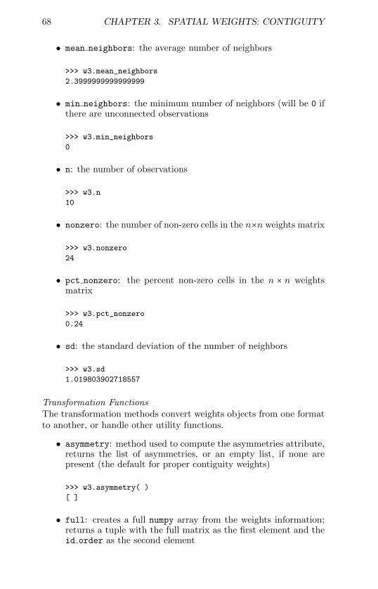
68 CHAPTER 3. SPATIAL WEIGHTS: CONTIGUITY
• mean neighbors: the average number of neighbors
>>> w3.mean_neighbors2.3999999999999999
• min neighbors: the minimum number of neighbors (will be 0 ifthere are unconnected observations
>>> w3.min_neighbors0
• n: the number of observations
>>> w3.n10
• nonzero: the number of non-zero cells in the n×n weights matrix
>>> w3.nonzero24
• pct nonzero: the percent non-zero cells in the n × n weightsmatrix
>>> w3.pct_nonzero0.24
• sd: the standard deviation of the number of neighbors
>>> w3.sd1.019803902718557
Transformation FunctionsThe transformation methods convert weights objects from one formatto another, or handle other utility functions.
• asymmetry: method used to compute the asymmetries attribute,returns the list of asymmetries, or an empty list, if none arepresent (the default for proper contiguity weights)
>>> w3.asymmetry( )[ ]
• full: creates a full numpy array from the weights information;returns a tuple with the full matrix as the first element and theid order as the second element

3.4. CONTIGUITY WEIGHTS IN PYSAL 69
>>> w3.full( )(array([[ 0., 0., 0., 0., 0., 0., 0., 0., 0., 0.],
[ 0., 0., 1., 0., 1., 0., 0., 0., 0., 0.],[ 0., 1., 0., 1., 0., 1., 0., 0., 0., 0.],[ 0., 0., 1., 0., 0., 0., 1., 0., 0., 0.],[ 0., 1., 0., 0., 0., 1., 0., 1., 0., 0.],[ 0., 0., 1., 0., 1., 0., 1., 0., 1., 0.],[ 0., 0., 0., 1., 0., 1., 0., 0., 0., 1.],[ 0., 0., 0., 0., 1., 0., 0., 0., 1., 0.],[ 0., 0., 0., 0., 0., 1., 0., 1., 0., 1.],[ 0., 0., 0., 0., 0., 0., 1., 0., 1., 0.]]),
[9, 0, 3, 6, 1, 4, 7, 2, 5, 8])
If one just wants the full array, the function needs to be sub-scripted by ([0]) as in
>>> w3.full( )[0]array([[ 0., 0., 0., 0., 0., 0., 0., 0., 0., 0.],
[ 0., 0., 1., 0., 1., 0., 0., 0., 0., 0.],[ 0., 1., 0., 1., 0., 1., 0., 0., 0., 0.],[ 0., 0., 1., 0., 0., 0., 1., 0., 0., 0.],[ 0., 1., 0., 0., 0., 1., 0., 1., 0., 0.],[ 0., 0., 1., 0., 1., 0., 1., 0., 1., 0.],[ 0., 0., 0., 1., 0., 1., 0., 0., 0., 1.],[ 0., 0., 0., 0., 1., 0., 0., 0., 1., 0.],[ 0., 0., 0., 0., 0., 1., 0., 1., 0., 1.],[ 0., 0., 0., 0., 0., 0., 1., 0., 1., 0.]])
• get transform: method to return the current weights transfor-mation, same e↵ect as the transform attribute
>>> w3.get_transform( )’B’
• set shapefile: method to record the items for a GAL headerfile, for internal use only
• set transform: method to set weights transformation to oneof ‘O’, ‘B’, ‘R’, or ’V’; same e↵ect as setting the transformattribute directly
>>> w3.transform = ’B’>>> w3.set_transform(’R’)>>> w3.transform’R’
• sparse: an attribute of the spatial weights object that containsa sparse numpy array representation of the weights, intended formanipulation as an array (not as a sparse spatial weights object,see towsp)

70 CHAPTER 3. SPATIAL WEIGHTS: CONTIGUITY
>>> w3.sparse<10x10 sparse matrix of type ’<type ’numpy.float64’>’with 24 stored elements in Compressed Sparse Row format>
• towsp: method to convert a regular spatial weights object to asparse spatial weights object (class WSP); the result is not just asparse numpy array (as for sparse), but an actual weights objectwith attributes
>>> ws = w3.towsp( )>>> ws<pysal.weights.weights.WSP at 0xb266930>
Auxiliarly VariablesA series of auxiliary variables are stored as attributes of a spatialweights object to facilitate the calculation of tests and diagnostics forspatial autocorrelation, such as Moran’s I and the Lagrange Multipliertests (see Section 5.1.6 of Chapter 5). Typically, these are not neededin and of themselves, but they can be investigated for pedagogicalpurposes, e.g., to illustrate the di↵erent components of the statisticalinference, such as expression tr(WW +W′W) in Equation 5.15.
• diagW2: the elements of the diagonal of the matrix WW
>>> w3.diagW2array([ 0. , 0.33333333, 0.41666667, 0.33333333,
0.41666667, 0.33333333, 0.41666667, 0.33333333,0.41666667, 0.33333333])
• diagWtW: the elements of the diagonal of the matrix W′W>>> w3.diagWtWarray([ 0. , 0.22222222, 0.5625 , 0.22222222,
0.5625 , 0.44444444, 0.5625 , 0.22222222,0.5625 , 0.22222222])
• diagWtW WW: the elements of the diagonal of the sum of matri-ces WW and W′W (i.e., the sum of the matching elements ofdiagW2 and diagWtW)
>>> w3.diagWtW_WWarray([ 0. , 0.55555556, 0.97916667, 0.55555556,
0.97916667, 0.77777778, 0.97916667, 0.55555556,0.97916667, 0.55555556])
• s0: the sum of all weights S0 = ∑i∑j wij ; note that in ourexample this is one less than the number of observations (9 = 10- 1) because of the unconnected unit, in normal circumstancesS0 = n for row-standardized weights

3.4. CONTIGUITY WEIGHTS IN PYSAL 71
>>> w3.s08.9999999999999982
• s1: S1 = ∑i∑j(wij +wji)2; not used in spatial econometrics
>>> w3.s16.9166666666666661
• s2: S2 = ∑j(∑iwij +∑iwji)2; not used in spatial econometrics
>>> w3.s236.80555555555555
• s2array: an array that constitutes an intermediate step in thecomputation of s2, consisting of the elements for each j (s2is the sum of the elements in this array); not used in spatialeconometrics
>>> w3.s2arrayarray([[ 0. ],
[ 2.77777778],[ 5.0625 ],[ 2.77777778],[ 5.0625 ],[ 5.44444444],[ 5.0625 ],[ 2.77777778],[ 5.0625 ],[ 2.77777778]])
• trcW2: the trace of the matrixWW, i.e., the sum of the elementsof diagW2
>>> w3.trcW23.3333333333333335
• trcWtW: the trace of the matrix W′W, i.e., the sum of the ele-ments of diagWtW
>>> w3.trcWtW3.5833333333333335
• trcWtW WW: the trace of the matrix WW +W′W, i.e., the sumof trcW2 and trcWtW
>>> w3.trcWtW_WW6.9166666666666661

72 CHAPTER 3. SPATIAL WEIGHTS: CONTIGUITY
3.4.1.3 The Sparse Spatial Weights Class WSP
In spreg, all the weights manipulations are carried out using sparsespatial weights objects. These are constructed under the hood andseldom need to be created explicitly. For completeness sake, we brieflydescribe the sparse spatial weights class WSP and its attributes.
We already saw one way to create a WSP object from a regularspatial weights object by means of the towsp method (see previousSection). The way to create such an object directly is:
>>> ws = pysal.WSP(sparse,id_order=None)
with as arguments:
• sparse: a matrix in a scipy sparse array format; required ar-gument
• id order: optional, the id order list, same as for a regularspatial weights object
The sparse array passed to WSP can be any sparse format supported byscipy. Internally, it is converted to a CSR (compressed sparse row)format, so this extra step can be avoided by passing a CSR array tobegin with.
We illustrate this by continuing to use our previous example, wherewe created the weights object w3. We saw in the previous Sectionhow we can extract a sparse array from this object using the sparseattribute. This array is in the CSR format, so we can use it as aninput to WSP.
>>> sparsemat = w3.sparse>>> sparsemat<10x10 sparse matrix of type ’<type ’numpy.float64’>’with 24 stored elements in Compressed Sparse Row format>>>> sparseW = pysal.weights.WSP(sparsemat,id_order=order_id)>>> sparseW<pysal.weights.weights.WSP at 0xb2f9490>
Of course, in practice, one will typically first create a regular spatialweights object and then convert it to a sparse object using the towspmethod. Finally, a sparse spatial weights object can be converted to aregular spatial weights object by means of the pysal.weights.WSP2Wfunction (see the online API reference for technical details).
3.4.1.4 Attributes of a Sparse Spatial Weights Object
Sparse spatial weights objects have only a small subset of the attributesof a regular weights object. They are intended to be manipulateddirectly as sparse matrices, so the attributes are limited to the ar-guments passed, id order, the number of observations, n, and two

3.4. CONTIGUITY WEIGHTS IN PYSAL 73
auxiliary variables, s0 and trcWtW WW. Their meaning is the same asfor a regular spatial weights object.
In our example:
>>> sparseW.id_order[9, 0, 3, 6, 1, 4, 7, 2, 5, 8]>>> sparseW.n10>>> sparseW.s08.9999999999999982>>> sparseW.trcWtW_WW6.9166666666666661
The other attributes of a weights object are not available and willgenerate an error message when requested. For example:
>>> sparseW.transformAttributeError Traceback (most recent call last)...----> 1 sparseW.transformAttributeError: ’WSP’ object has no attribute ’transform’
3.4.2 Creating Contiguity Weights from a Shape-file
Spatial weights objects based on the contiguity between polygons canbe created directly from ESRI shape files. PySAL currently supportsboth queen and rook, as well as higher order contiguity.6
3.4.2.1 Queen Contiguity Weights
In PySAL, queen contiguity weights are constructed by means of thespecial user function queen from shapefile . The only mandatoryargument for this function is the filename for the shape file, includingthe shp file extension. When the shape file is not present in the cur-rent working directory, the full pathname needs to be specified. Thecomplete call is:
>>> w = pysal.queen_from_shapefile(shapefile, idVariable=None,sparse=False)
The optional arguments are:
• idVariable: a variable from the data base associated with theshape file (the dbf file) to be used as an ID variable for theweights
6The contiguity extraction algorithms in PySAL assume the shapefile respectsplanar enforcement, requiring that no polygons overlap and that any lines must besplit at points of intersection.

74 CHAPTER 3. SPATIAL WEIGHTS: CONTIGUITY
• sparse: a boolean flag to indicate whether a regular spatialweights object is created (False, the default) or a sparse spatialweights object (True)
The function returns a spatial weights object, either a regular one(the default), or a sparse spatial weights object for sparse = True.These objects have all the attributes discussed previously, respectivelyin Section 3.4.1.2 for regular weights and in Section 3.4.1.4 for sparseweights.
To illustrate this, we again take the U.S. county NAT.shp datafrom the PySAL examples set. We use the pysal.examples.get pathfunction to make sure the proper path name is prefixed to the nameof the shape file. We set the idVariable to FIPSNO (this is the sameapproach as taken for GeoDa and GeoDaSpace). The full call is then:
>>> wq = pysal.queen_from_shapefile(pysal.examples.get_path(’NAT.shp’),idVariable=’FIPSNO’)
>>> wq<pysal.weights.weights.W at 0xb3c2510>
It is clear that wq is a spatial weights object.It is important to keep in mind that the spatial object created from
the shape file has binary weights. This is not directly obvious, sincethe transform attribute is initially set to ’O’:
>>> wq.transform’O’
but the weights are binary, for, example, for observation with FIPSNO= 27077:
>>> wq.weights[27077][1.0, 1.0, 1.0]
It is therefore critical to always follow the creation of the weightsobject by an explicit row-standardization:
>>> wq.transform = ’R’>>> wq.weights[27077][0.3333333333333333, 0.3333333333333333, 0.3333333333333333]
With the sparse flag set to True, the resulting object is a sparsespatial weights object. For example:
>>> wqsparse = pysal.queen_from_shapefile(pysal.examples.get_path(’NAT.shp’),idVariable=’FIPSNO’,sparse=True)
>>> wqsparse<pysal.weights.weights.WSP at 0x9a67830>
Note that these weights are binary:

3.4. CONTIGUITY WEIGHTS IN PYSAL 75
>>> wqsparse.s018168.0
If the weights were row-standardized, s0 should equal the numberof observations, n = 3085, so clearly in this case, they are not. Inorder to get sparse spatial weights objects into row-standardize form,a better approach is to create a regular spatial weights object, sayw, convert it to row-standardized form using w.transform = ’R’ andthen obtain a sparse spatial weights object from w.towsp( ).
3.4.2.2 Rook Contiguity Weights
Rook contiguity weights are constructed from a shape file by means ofthe user function rook from shapefile. The complete call is identicalto that for queen weights, except that a di↵erent function name is used:
>>> wr = pysal.rook_from_shapefile(shapefile, idVariable=None,sparse=False)
The arguments and options are the same as those covered in Sec-tion 3.4.2.1, and they will not be repeated here.
3.4.3 Creating Weights for a Regular Lattice Struc-ture
PySAL includes functionality to generate a spatial weights object di-rectly for any rectangular or hexagonal lattice structure.7 This is oftenvery useful in the context of simulation experiments. Since the neigh-bor structure of the lattice is known, there is no need to construct itby reading the contents of a shape file.
For a rectangular lattice, the function is lat2W, invoked as:
>>> wgrid = pysal.lat2W(nrows=5,ncols=5,rook=True,id_type=’int’)
This function returns a standard spatial weights object.8 Without anyarguments, i.e., pysal.lat2W( ), this results in the weights for a 5×5regular grid, i.e., a 25 × 25 weights matrix. The four arguments are:
• nrows: the number of rows in the grid, default is 5
• ncols: the number of columns in the grid, default is 5
• rook: the type of contiguity, default is True for rook contiguity
7Note that this functionality is not available through the GUI of GeoDa orGeoDaSpace.
8PySAL also contains a function that creates a sparse spatial weights object fora regular lattice: pysal.weights.lat2SW. See the online API reference for details.

76 CHAPTER 3. SPATIAL WEIGHTS: CONTIGUITY
• id type: the representation of the ID variable, either as an inte-ger, starting with 0 (’int’), as a real variable, starting with 0.0(’float’), or as a simple string, starting with ’id0’ (’string’)
We return to the 3 × 3 lattice we used as an example before, andexplore the three options for the id type. First, the default case, usinginteger values:
>>> w3x3 = pysal.lat2W(3,3)>>> w3x3.weights{0: [1.0, 1.0],1: [1.0, 1.0, 1.0],2: [1.0, 1.0],3: [1.0, 1.0, 1.0],4: [1.0, 1.0, 1.0, 1.0],5: [1.0, 1.0, 1.0],6: [1.0, 1.0],7: [1.0, 1.0, 1.0],8: [1.0, 1.0]}
next, using real valued IDs (the key in the weights dictionary):
>>> w3x3f = pysal.lat2W(3,3,id_type=’float’)>>> w3x3f.weights{0.0: [1.0, 1.0],1.0: [1.0, 1.0, 1.0],2.0: [1.0, 1.0],3.0: [1.0, 1.0, 1.0],4.0: [1.0, 1.0, 1.0, 1.0],5.0: [1.0, 1.0, 1.0],6.0: [1.0, 1.0],7.0: [1.0, 1.0, 1.0],8.0: [1.0, 1.0]}
and finally, for strings:
>>> w3x3s = pysal.lat2W(3,3,id_type=’string’)>>> w3x3s.weights{’id0’: [1.0, 1.0],’id1’: [1.0, 1.0, 1.0],’id2’: [1.0, 1.0],’id3’: [1.0, 1.0, 1.0],’id4’: [1.0, 1.0, 1.0, 1.0],’id5’: [1.0, 1.0, 1.0],’id6’: [1.0, 1.0],’id7’: [1.0, 1.0, 1.0],’id8’: [1.0, 1.0]}
A similar function for hexagonal grids is pysal.hexLat2W. For furthertechnical details, we refer to the online API reference.

3.4. CONTIGUITY WEIGHTS IN PYSAL 77
3.4.4 Block Weights
A particular form of contiguity weights are the block weights intro-duced in Section 3.1.2. PySAL supports the creation of these weights,but neither GeoDa or GeoDaSpace currently do. The function thataccomplishes this is regime weights. The full call is:
>>> wreg = pysal.regime_weights(regimes)
with one required argument:
• regimes: a list or numpy array matching the observations, withfor each observation the regime it belongs to.
The identifiers for the regimes can be numeric, unique integers orunique floats, or strings (unique for each regime). The result is aspatial weights object in binary form (i.e., not with row-standardizedweights).
To illustrate this, consider a list for a data set with 15 observationsand three regimes, indicated by ’s’, ’e’ and ’w’. The list is:
>>> regimes = [’s’, ’s’, ’s’, ’s’, ’s’,’e’, ’e’, ’e’, ’e’, ’e’,’w’, ’w’, ’w’, ’w’, ’w’]
The block weights are created as:
>>> wreg = pysal.regime_weights(regimes)
with the following neighbor structure:
>>> wreg.neighbors{0: [1, 2, 3, 4],1: [0, 2, 3, 4],2: [0, 1, 3, 4],3: [0, 1, 2, 4],4: [0, 1, 2, 3],5: [6, 7, 8, 9],6: [5, 7, 8, 9],7: [5, 6, 8, 9],8: [5, 6, 7, 9],9: [5, 6, 7, 8],10: [11, 12, 13, 14],11: [10, 12, 13, 14],12: [10, 11, 13, 14],13: [10, 11, 12, 14],14: [10, 11, 12, 13]}
Each of the observations is a neighbor to the other observations in thesame block, but not to any outside the block.

78 CHAPTER 3. SPATIAL WEIGHTS: CONTIGUITY
3.4.5 Higher Order Contiguity
Once a first order contiguity spatial weights object is available, higherorder contiguity can be obtained in a straightforward manner. ThePySAL higher order function takes as arguments a weights objectand the order of contiguity (as an integer).9 The complete call is:
w_high = pysal.higher_order(w, k = 2)
where
• w: a regular (i.e., not sparse) spatial weights object, required
• k: the order of contiguity, default k = 2
This returns a spatial weights object with the higher order contiguity,using the same Anselin and Smirnov (1996) algorithm as GeoDa. How-ever, in contrast to the implementation in GeoDa and GeoDaSpace,there is no option to include lower order neighbors. This must becarried out explicitly by means of the PySAL w union function:
w_combined = pysal.w_union(w1, w2,silent_island_warning = False)
The required arguments to this function are two (non-sparse) spatialweights objects. Optional is a flag for the silent island warningwhich has the same meaning as in the construction of a spatial weightsobject (see Section 3.4.1.1). It returns a new spatial weights object(with binary weights) in which the neighbor structures of the two ar-guments are combined (union). In the special case of higher order con-tiguity weights, this must be implemented in multiple steps, graduallybuilding up the weights structure until the desired order is achieved.For example, if second order contiguity with lower order neighbors isdesired, this is accomplished by applying w union to the first and sec-ond order weights. However, for higher orders, such as third, the firstand second need to be combined first, then the combined weights needto be merged with the third order contiguity, in a step-wise fashion.
We illustrate this for the queen contiguity weights we created inSection 3.4.2.1. Second order contiguity follows as:
>>> wq2 = pysal.higher_order(wq,k=2)
and including the first order neighbors from:
>>> wq2include = pysal.w_union(wq,wq2)
9The PySAL function pysal.weights.higher order sp implements higher ordercontiguity for sparse weights objects. See the online API reference for technicaldetails.

3.4. CONTIGUITY WEIGHTS IN PYSAL 79
We now compare the neighbors for observation with FIPSNO = 53019in the first order contiguity weights and the two higher order weights(see also lines 3-4 in the GAL file of Figure 3.5 for the first orderneighbors of FIPSNO = 53019):
>>> wq.neighbors[53019][53065, 53043, 53047]>>> wq2.neighbors[53019][53071, 53077, 12131, 4001, 4025, 45003, 45009, 45021, 45025]>>> wq2include.neighbors[53019][4001, 12131, 45025, 53065, 45003, 53071, 45009,53043, 53077, 53047, 4025, 45021]
As expected, the neighbors for wq2include combine the lists for thefirst and second order contiguity weights.
3.4.6 Reading Weights Files
Arguably, the most straightforward way to create a spatial weightsobject in PySAL is to read its content from a pre-existing file. Aspreviously shown in Figure 3.14, PySAL currently supports 11 weightsfile formats. Reading a weights file operates in the same manner asreading any other file in PySAL and is based on the FILEIO module. Itoperates in three basic steps: (i) create a file handle to open the filefor reading; (ii) read the contents and convert into a spatial weightsobject; and (iii) close the file.
We illustrate this using the nat queen.gal queen contiguity filefor the U.S. counties that we created with GeoDa in Section 3.2.2.1. Apartial glance at its contents is given in Figure 3.5.
The three steps to read this GAL file into a spatial weights objectare:
>>> galw = pysal.open(pysal.examples.get_path(’nat_queen.gal’),’r’)
>>> w = galw.read()>>> galw.close()
We now have the spatial weights object w and we can check its at-tributes in the usual fashion. For example, the dimension is foundas:
>>> w.n3085
The neighbors and weights for ID = ’27077’ are:
>>> w.neighbors[’27077’][’27007’, ’27135’, ’27071’]>>> w.weights[’27077’][1.0, 1.0, 1.0]

80 CHAPTER 3. SPATIAL WEIGHTS: CONTIGUITY
Note that the weights are binary, so that an explicit row-standardizationalways needs to be carried out before using the weights in spatial re-gression operations. Also, the ID variable is interpreted as a string,rather than an integer, hence the need to surround the value by quotes.It is good practice to check the nature of the ID variable by listing partof the id order attribute. For example:
>>> w.id_order[:3][’27077’, ’53019’, ’53065’]
Weights files created in other formats are read in the same fashion,by using the open and read commands on the file (with full path namespecified if needed) with the ’r’ option. PySAL internally recognizesthe file extension and uses the appropriate file reader for that format.
3.4.7 Writing and Converting Weights Files
Weights objects created in PySAL can be written out to files in arange of supported formats (see Figure 3.14). The file extension de-termines the format that will be used. For example, assuming wecreated the file object w by reading from the file nat queen.gal (asin Section 3.4.6), its contents can be written to a GAL format file bymeans of the open and write commands on the file (with full pathname specified if needed), with the ’w’ option and the weights object(w) specified as the argument of the write function. In our exam-ple, using natqueen1.gal as the file name for the output file, this isaccomplished with:
>>> galwout = pysal.open("natqueen1.gal",’w’)>>> galwout.write(w)>>> galwout.close()
The first few lines of the natqueen1.gal file are as follows:
308527077 327007 27135 2707153019 353047 53065 5304353065 453043 53051 53063 53019
Note how the original header line is replaced by a single item, thenumber of observations (3085). In all other respects, the file is identicalto the input file.
PySAL also contains functionality to convert between weights for-mats directly, using the pysal.weight convert command. However,this will typically not be necessary, since a weights object can be readfrom any supported format and subsequently written to a file in any