Modern regression 2: The lasso

Ryan TibshiraniData Mining: 36-462/36-662

March 21 2013

Optional reading: ISL 6.2.2, ESL 3.4.2, 3.4.3

1

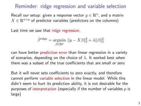
Reminder: ridge regression and variable selection

Recall our setup: given a response vector y ∈ Rn, and a matrixX ∈ Rn×p of predictor variables (predictors on the columns)

Last time we saw that ridge regression,

βridge = argminβ∈Rp

‖y −Xβ‖22 + λ‖β‖22

can have better prediction error than linear regression in a varietyof scenarios, depending on the choice of λ. It worked best whenthere was a subset of the true coefficients that are small or zero

But it will never sets coefficients to zero exactly, and thereforecannot perform variable selection in the linear model. While thisdidn’t seem to hurt its prediction ability, it is not desirable for thepurposes of interpretation (especially if the number of variables p islarge)

2

Recall our example: n = 50, p = 30; true coefficients: 10 arenonzero and pretty big, 20 are zero

0 5 10 15 20 25

0.0

0.2

0.4

0.6

0.8

λ

Linear MSERidge MSERidge Bias^2Ridge Var

0 5 10 15 20 25

−0.

50.

00.

51.

0

λ

Coe

ffici

ents

●

●

●

●

●

●

●●

●

●

●

●

●

●

●

●

●

●

●

●

●

●

●●

●

●

●

●

●

●

True nonzeroTrue zero

3

Example: prostate data

Recall the prostate data example: we are interested in the level ofprostate-specific antigen (PSA), elevated in men who have prostatecancer. We have measurements of PSA on n = 97 men withprostate cancer, and p = 8 clinical predictors. Ridge coefficients:

0 200 400 600 800 1000

0.0

0.2

0.4

0.6

λ

Coe

ffici

ents

●

●

●

●

●

●

●

●

lcavol

lweight

age

lbph

svi

lcp

gleason

pgg45

0 2 4 6 8

0.0

0.2

0.4

0.6

df(λ)

Coe

ffici

ents

●

●

●

●

●

●

●

●

lcavol

lweight

age

lbph

svi

lcp

gleason

pgg45

What if the people who gave this data want us to derive a linearmodel using only a few of the 8 predictor variables to predict thelevel of PSA?

4

Now the lasso coefficient paths:

0 20 40 60 80

0.0

0.2

0.4

0.6

λ

Coe

ffici

ents

●

●

●

●

●

●

●

●

lcavol

lweight

age

lbph

svi

lcp

gleason

pgg45

0 2 4 6 8

0.0

0.2

0.4

0.6

df(λ)

Coe

ffici

ents

●

●

●

●

●

●

●

●

lcavol

lweight

age

lbph

svi

lcp

gleason

pgg45

We might report the first 3 coefficients to enter the model: lcavol(the log cancer volume), svi (seminal vesicle invasion), and lweight(the log prostate weight)

How would we choose 3 (i.e., how would we choose λ?) We’ll talkabout this later

5

The lasso

The lasso1 estimate is defined as

βlasso = argminβ∈Rp

‖y −Xβ‖22 + λ

p∑j=1

|βj |

= argminβ∈Rp

‖y −Xβ|22︸ ︷︷ ︸Loss

+λ ‖β‖1︸︷︷︸Penalty

The only difference between the lasso problem and ridge regressionis that the latter uses a (squared) `2 penalty ‖β‖22, while theformer uses an `1 penalty ‖β‖1. But even though these problemslook similar, their solutions behave very differently

Note the name “lasso” is actually an acronym for: Least AbsoluteSelection and Shrinkage Operator

1Tibshirani (1996), “Regression Shrinkage and Selection via the Lasso”6

βlasso = argminβ∈Rp

‖y −Xβ‖22 + λ‖β‖1

The tuning parameter λ controls the strength of the penalty, and(like ridge regression) we get βlasso = the linear regression estimatewhen λ = 0, and βlasso = 0 when λ =∞

For λ in between these two extremes, we are balancing two ideas:fitting a linear model of y on X, and shrinking the coefficients.But the nature of the `1 penalty causes some coefficients to beshrunken to zero exactly

This is what makes the lasso substantially different from ridgeregression: it is able to perform variable selection in the linearmodel. As λ increases, more coefficients are set to zero (lessvariables are selected), and among the nonzero coefficients, moreshrinkage is employed

7

Example: visual representation of lasso coefficients

Our running example from last time: n = 50, p = 30, σ2 = 1, 10large true coefficients, 20 small. Here is a visual representation oflasso vs. ridge coefficients (with the same degrees of freedom):

−0.5 0.0 0.5 1.0 1.5 2.0 2.5

0.0

0.5

1.0

Coe

ffici

ents

●

●

●

●

●

●

●

●

●

●

●

●

●

●●●

●

●

●

●

●

●●

●

●●●

●

●

●

●

●

●

●

●

●

●

●●

●

●

●●

●●

●

●

●●

●

●

●

●●

●●

●●

●●

●

●

●●

●

●

●

●●

●

●

●●●●●

●

●●

●●

●●●●●●●●●

True Ridge Lasso

8

Important details

When including an intercept term in the model, we usually leavethis coefficient unpenalized, just as we do with ridge regression.Hence the lasso problem with intercept is

β0, βlasso = argmin

β0∈R, β∈Rp‖y − β01−Xβ‖22 + λ‖β‖1

As we’ve seen before, if we center the columns of X, then theintercept estimate turns out to be β0 = y. Therefore we typicallycenter y,X and don’t include an intercept them

As with ridge regression, the penalty term ‖β‖1 =∑p

j=1 |βj | is notfair is the predictor variables are not on the same scale. Hence, ifwe know that the variables are not on the same scale to beginwith, we scale the columns of X (to have sample variance 1), andthen we solve the lasso problem

9

Bias and variance of the lasso

Although we can’t write down explicit formulas for the bias andvariance of the lasso estimate (e.g., when the true model is linear),we know the general trend. Recall that

βlasso = argminβ∈Rp

‖y −Xβ‖22 + λ‖β‖1

Generally speaking:

I The bias increases as λ (amount of shrinkage) increases

I The variance decreases as λ (amount of shrinkage) increases

What is the bias at λ = 0? The variance at λ =∞?

In terms of prediction error (or mean squared error), the lassoperforms comparably to ridge regression

10

Example: subset of small coefficients

Example: n = 50, p = 30; true coefficients: 10 large, 20 small

0 2 4 6 8 10

0.0

0.2

0.4

0.6

0.8

λ

Linear MSELasso MSELasso Bias^2Lasso Var

The lasso: see the function lars in the package lars

11

Example: all moderate coefficients

Example: n = 50, p = 30; true coefficients: 30 moderately large

0 2 4 6 8 10

0.0

0.5

1.0

1.5

2.0

λ

Linear MSELasso MSELasso Bias^2Lasso Var

Note that here, as opposed to ridge regression the variance doesn’tdecrease fast enough to make the lasso favorable for small λ

12

Example: subset of zero coefficients

Example: n = 50, p = 30; true coefficients: 10 large, 20 zero

0 2 4 6 8 10 12

0.0

0.2

0.4

0.6

0.8

λ

Linear MSELasso MSELasso Bias^2Lasso Var

13

Advantage in interpretation

On top the fact that the lasso is competitive with ridge regressionin terms of this prediction error, it has a big advantage with respectto interpretation. This is exactly because it sets coefficients exactlyto zero, i.e., it performs variable selection in the linear model

Recall the prostate cancer data example:

0 200 400 600 800 1000

0.0

0.2

0.4

0.6

λ

Coe

ffici

ents

●

●

●

●

●

●

●

●

lcavol

lweight

age

lbph

svi

lcp

gleason

pgg45

0 20 40 60 80

0.0

0.2

0.4

0.6

λ

Coe

ffici

ents

●

●

●

●

●

●

●

●

lcavol

lweight

age

lbph

svi

lcp

gleason

pgg45

14

Example: murder data

Example: we study the murder rate (per 100K people) of n = 2215communities in the U.S.2 We have p = 101 attributes measuredeach community, such as

[1] "racePctHisp "agePct12t21" "agePct12t29"

[4] "agePct16t24" "agePct65up" "numbUrban"

[7] "pctUrban" "medIncome" "pctWWage"

...

Our goal is to predict the murder rate as a linear function of theseattributes. For the purposes of interpretation, it would be helpfulto have a linear model involving only a small subset of theseattributes. (Note: interpretation here is not causal)

2Data from UCI Machine Learning Repository, http://archive.ics.uci.edu/ml/datasets/Communities+and+Crime+Unnormalized

15

With ridge regression, regardless of the choice of λ <∞, we neverget zero coefficient estimates. For λ = 25, 000, which correspondsto approximately 5 degrees of freedom, we get estimates:

racePctHisp agePct12t21 agePct12t29

0.0841354923 0.0076226029 0.2992145264

agePct16t24 agePct65up numbUrban

-0.2803165408 0.0115873137 0.0154487020

pctUrban medIncome pctWWage

-0.0155148961 -0.0105604035 -0.0228670567

...

With the lasso, for about the same degrees of freedom, we get:

agePct12t29 agePct16t24 NumKidsBornNeverMar

0.7113530 -1.8185387 -0.6835089

PctImmigRec10 OwnOccLowQuart

1.3825129 1.0234245

and all other coefficient estimates are zero. That is, we get exactly5 nonzero coeffcients out of p = 101 total

16

Example: credit data

Example from ISL sections 6.6.1 and 6.6.2: response is averagecredit debt, predictors are income, limit (credit limit), rating(credit rating), student (indicator), and others

Ridge Lasso

17

Constrained form

It can be helpful to think of our two problems constrained form:

βridge = argminβ∈Rp

‖y −Xβ‖22 subject to ‖β‖22 ≤ t

βlasso = argminβ∈Rp

‖y −Xβ‖22 subject to ‖β‖1 ≤ t

Now t is the tuning parameter (before it was λ). For any λ andcorresponding solution in the previous formulation (sometimescalled penalized form), there is a value of t such that the aboveconstrained form has this same solution

In comparison, the usual linear regression estimate solves theunconstrained least squares problem; these estimates constrain thecoefficient vector to lie in some geometric shape centered aroundthe origin. This generally reduces the variance because it keeps theestimate close to zero. But which shape we choose really matters!

18

Why does the lasso give zero coefficients?

(From page 71 of ESL)

19

What is degrees of freedom?

Broadly speaking, the degrees of freedom of an estimate describesits effective number of parameters

More precisely, given data y ∈ Rn from the model

yi = µi + εi, i = 1, . . . n

where E[εi] = 0, Var(εi) = σ2, Cov(εi, εj) = 0, suppose that weestimate y by y. The degrees of freedom of the estimate y is

df(y) =1

σ2

n∑i=1

Cov(yi, yi)

The higher the correlation between the ith fitted value and the ithdata point, the more adaptive the estimate, and so the higher itsdegrees of freedom

20

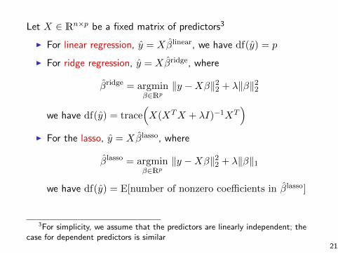
Let X ∈ Rn×p be a fixed matrix of predictors3

I For linear regression, y = Xβlinear, we have df(y) = p

I For ridge regression, y = Xβridge, where

βridge = argminβ∈Rp

‖y −Xβ‖22 + λ‖β‖22

we have df(y) = trace(X(XTX + λI)−1XT

)I For the lasso, y = Xβlasso, where

βlasso = argminβ∈Rp

‖y −Xβ‖22 + λ‖β‖1

we have df(y) = E[number of nonzero coefficients in βlasso]

3For simplicity, we assume that the predictors are linearly independent; thecase for dependent predictors is similar

21

One usage of degrees of freedom is to put two different estimateson equal footing

E.g., comparing ridge and lasso for the prostate cancer data set

Ridge Lasso

0 2 4 6 8

0.0

0.2

0.4

0.6

df(λ)

Coe

ffici

ents

●

●

●

●

●

●

●

●

lcavol

lweight

age

lbph

svi

lcp

gleason

pgg45

0 2 4 6 8

0.0

0.2

0.4

0.6

df(λ)

Coe

ffici

ents

●

●

●

●

●

●

●

●

lcavol

lweight

age

lbph

svi

lcp

gleason

pgg45

22

Recap: the lasso

In this lecture we learned a variable selection method in the linearmodel setting: the lasso. The lasso uses a penalty like ridgeregression, except the penalty is the `1 norm of the coefficientvector, which causes the estimates of some coefficients to beexactly zero. This is in constrast to ridge regression which neversets coefficients to zero

The tuning parameter λ controls the strength of the `1 penalty.The lasso estimates are generally biased, but have good meansquared error (comparable to ridge regression). On top of this, thefact that it sets coefficients to zero can be a big advantage for thesake of interpretation

We defined the concept of degrees of freedom, which measures theeffective number of parameters used by a estimator. This allows usto compare estimators with different tuning parameters

23

Next time: model selection and validation

Cross-validation can be used to estimate the prediction error curve

(From ESL page 244)

24