Lecture notes for the spring semester of 2005

MODERN PHYSICS

Fam Le Kien

Department of Applied Physics and Chemistry,

University of Electro-Communications, Chofu, Tokyo 182-8585, Japan

Textbook: CONCEPTS OF MODERN PHYSICS (sixth edition, 2003)

By Arthur Beiser

McGraw-Hill

i

Contents

I. The special theory of relativity 1

A. The Michelson-Morley experiment 1

B. The special theory of relativity 4

C. The Galilean transformation 5

D. The Lorentz transformation 7

E. Length contraction 9

F. Time dilation 11

G. Doppler effect 13

1. Doppler effect in sound 13

2. Doppler effect in light 14

H. The relativity of mass 15

I. Mass and energy 18

J. Velocity addition 21

II. Wave properties of particles 23

A. De Broglie waves 23

B. Wave function: de Broglie waves are waves of probability amplitude 24

C. Describing a wave 25

D. Phase and group velocities of de Broglie waves 27

III. Particle diffraction 32

IV. Uncertainty principle 37

Average value and standard deviation 40

Compatible observables 40

Proof of the uncertainty principle 40

Uncertainty principle from the particle approach 41

Uncertainty principle for energy and time 42

V. Atomic spectra 46

A. Spectral series 46

B. The Bohr atom 47

ii

C. Energy levels and spectra 50

D. Origin of line spectra 51

VI. Correspondence principle 55

VII. The lasers 57

VIII. Quantum mechanics 61

IX. Schrodinger equation 64

X. Particle in a box 69

XI. Finite potential well 75

XII. Tunnel effect 79

iii

I. THE SPECIAL THEORY OF RELATIVITY

A. The Michelson-Morley experiment

In the past, it was assumed that light is a wave propagating in an all-pervading elastic

medium called the ether. In other words, it was assumed that there exists a universal frame

of reference. Let us see what this idea means by considering a simple analogy.

Consider a river of width D which flows with the speed v, see Fig. 1. Two boats start

out from one bank of the river with the same speed V (with respect to the water). Boat

A crosses the river to a point on the other bank directly opposite the starting point and

then returns to the starting point. Boat B heads downstream for the distance D and then

returns to the starting point. Let’s calculate the time required for each round trip.

We first consider boat A. In order to compensate the water current, boat A must head

somewhat upstream, see Fig. 2. The upstream component of the velocity of boat A should

be exactly −v in order to cancel out the river current v. The perpendicular component V ′

is the actual speed across the river. We have the relation

V 2 = V ′2 + v2. (1)

Hence, the actual speed across the river is

V ′ =√

V 2 − v2 = V√

1− v2/V 2. (2)

The time for the initial crossing is D/V ′. The total round-trip time tA is twice D/V ′, that

is,

tA =2D/V√

1− v2/V 2. (3)

The case of boat B is somewhat different. As boat B heads downstream, its speed relative

to the shore is V + v, and it travels the distance D in the time

D

V + v. (4)

On the return trip, the speed of boat B relative to the shore is V − v, and boat B travels

the distance D in the timeD

V − v. (5)

1

FIG. 1: Boat A goes directly across the river and returns to its starting point, while boat B heads

downstream for an identical distance and then returns.

FIG. 2: Boat A must head upstream in order to compensate for the river current.

The total round-trip time tB is the sum of these times, namely,

tB =D

V + v+

D

V − v=

2D/V

1− v2/V 2. (6)

The ratio between the times tA and tB is

tAtB

=√

1− v2/V 2. (7)

If we know the common speed V of the two boats and measure the ratio tA/tB, we can

determine the speed v of the river current.

2

ether current

FIG. 3: The Michelson-Morley experiment.

The reasoning used in this problem may be transferred to the analogous problem of the

passage of light waves through the ether. If there is an ether pervading space, we move

through it with at least the speed of the earth’s orbital motion about the sun. From the

point of view of an observer on the earth, the ether is moving past the earth. To detect this

motion, we can use a pair of light beams formed by a beamsplitter instead of a pair of boats,

see Fig. 3. One of these light beams is directed to a mirror along a path perpendicular to the

ether current. The other beam goes to a mirror along a path parallel to the ether current.

The optical arrangement is such that both beams return to the same viewing screen. The

path lengths of the two beams are chosen to be exactly the same.

If there is no ether current, the two beams will arrive at the screen in phase and will

interfere constructively to yield a bright field of view. The presence of an ether current,

however, would cause the beams to have different transit times, so that they would no

longer arrive at the screen in phase but would interfere destructively. This is the essence of

the famous experiment performed by American physicists Michelson and Morley in 1887.

In the Michelson-Morley experiment, although the sensitivity was enough to detect the

expected ether current, no ether current was detected.

The negative result of the Michelson-Morley experiment had two consequences. First, it

3

said that the hypothesis of the ether is wrong. Second, it suggested that the speed of light

in free space is the same everywhere, regardless of any motion of the source or the observer.

B. The special theory of relativity

When we speak of motion, we mean motion relative to a frame of reference. Without a

frame of reference the concept of motion has no meaning. The frame of reference may be

a road, the earth’s surface, the sun, the center of our galaxy; but in every case we must

specify it. The absence of an ether means that there is no universal frame of reference.

Therefore, all motion exists solely relative to the person or instrument observing it. Should

we be isolated in the universe, there would be no way in which we could determine whether

we are in motion or not.

Inertial frame of reference: An inertial frame of reference is a frame in which Newton’s

first law of motion holds true. In such a frame, an object at rest remains at rest and an

object in motion continues to move at constant velocity if no force acts on it. Any frame

of reference that moves at constant velocity with respect to an inertial frame is itself an

inertial frame.

The special theory of relativity, developed by Einstein in 1905, treats problems involving

the motion of inertial frames of references at constant velocity with respect to one another.

It has a profound influence on all of physics.

The special theory of relativity is based upon two postulates:

1) The first postulate: The laws of physics may be expressed in equations having the

same form in all inertial frames of reference moving at constant velocity with respect to one

another. This postulate expresses the absence of a universal frame of reference.

2) The second postulate: The speed of light in free space has the same value in all inertial

frames of reference. This postulate follows directly from the result of the Michelson-Morley

experiment.

The above postulates subvert almost all of the intuitive concepts of time and space we

form on the basis of our daily experience. A simple example will illustrate this statement.

Example: We have two boats on a lake, with boat A stationary in the water and boat B

drifts at the constant velocity v. At the instant that B is abreast of A, a flare is fired by

somebody on one of the boats. The light from the flare travels uniformly in all directions,

4

according to the second postulate of special relativity. An observer in either boat must see a

sphere of light expanding with himself at its center, even though one of the boat is changing

its position with respect to the point where the flare went off.

The above situation is unusual. Why? Let us consider a more familiar analog. Instead

of firing a flare, one of the observers drops a stone into water when the boats are abreast of

each other. A circular pattern of ripples spreads out. The center of the circular pattern is

the point where the stone was dropped. Therefore, the pattern appears different to observers

on each boat.

It is important to recognize that motion and waves in water are entirely different from

motion and waves of light in space; water is in itself a frame of reference while space is not,

and the wave speed in water varies with the observer’s motion while the wave speed of light

does not.

C. The Galilean transformation

Suppose that we are in a frame of reference S and find that an event occurs at the time

t and has the coordinates x, y, z. Consider a different frame of reference S ′ moving with

respect to S at the constant velocity v, see Fig. 4. An observer located in S ′ will find

that the same event occurs at the time t′ and has the coordinates x′, y′, z′. How are the

measurements x, y, z, t related to x′, y′, z′, t′.

For simplicity, we assume that v is in the +x direction and that time in both systems is

measured from the instant when the origins of S and S ′ coincide. We intuitively expect that

the measurement x will exceed the measurement x′ by the amount vt while the measurements

y, z, t are the same as the measurements y′, z′, t′:

x′ = x− vt,

y′ = y,

z′ = z.

(8)

We also intuitively expect that times are the same in both frames of reference:

t′ = t. (9)

The set of equations (8) and (9) is known as the Galilean transformation.

5

FIG. 4: Frame S′ moves in the +x direction with the speed v relative to frame S.

To convert velocity components measured in the frame S to their equivalents in the frame

S ′, we simply differentiate Eqs. (8) with respect to time. The results are

V ′x = Vx − v,

V ′y = Vy,

V ′z = Vz.

(10)

The Galilean transformation and the corresponding velocity transformation are in accord

with our intuitive expectations. However, they violate both of the postulates of special

relativity. The first postulate calls for identical equations of physics in both the S and S ′

frames of reference, but the fundamental equations of electricity and magnetism assume

very different forms when Eqs. (8) and (9) are used. The second postulate calls for the

same value of the speed of light whether determined in S or S ′. If the speed of light in

the direction x in the S system is c, then in the system S ′ we have c′ = c − v, not correct.

Clearly, a different transformation is required if the postulates of special relativity are to be

satisfied.

6

D. The Lorentz transformation

We now develop a set of transformation equations directly from the postulates of special

relativity. A reasonable guess is

x′ = k(x− vt), (11)

where k is a factor of proportionality that does not depend on x and t but may be a function

of v. The choice of Eq. (11) follows from several considerations: it is linear in x and x′, so

that a single event in the frame S corresponds to a single event in the frame S ′; it is simple;

and it has the possibility of reducing to the equation x′ = x− vt, which is valid in ordinary

mechanics. Because the equations of physics must have the same form in both S and S ′, we

need only change the sign of v to write the corresponding equation for x in terms of x′ and

t′:

x = k(x′ + vt′). (12)

As in the case of the Galilean transformation, there is nothing to indicate that there

might be differences between y and y′ and between z and z′. Hence we again take

y′ = y

z′ = z.(13)

To get the time transformation, we substitute Eq. (11) into Eq. (94). The result is

x = k2(x− vt) + kvt′, (14)

from which we find that

t′ = kt +1− k2

kvx. (15)

To find k, we use the second postulate. At the instant t = t′ = 0, the origins of the two

frames of reference S and S ′ are in the same place. Suppose that a flare is set off at the

common origin at t = t′ = 0, and the observers in each system proceed to measure the speed

with which the light spreads out. Both observers must find the same speed c, which means

that the light propagation in the frames S and S ′ is governed by the equations

x = ct (16)

and

x′ = ct′, (17)

7

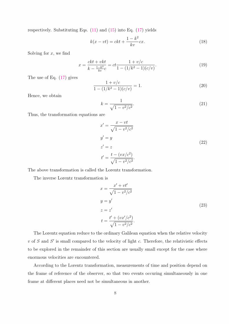
respectively. Substituting Eqs. (11) and (15) into Eq. (17) yields

k(x− vt) = ckt +1− k2

kvcx. (18)

Solving for x, we find

x =ckt + vkt

k − 1−k2

kvc

= ct1 + v/c

1− (1/k2 − 1)(c/v). (19)

The use of Eq. (17) gives1 + v/c

1− (1/k2 − 1)(c/v)= 1. (20)

Hence, we obtain

k =1√

1− v2/c2. (21)

Thus, the transformation equations are

x′ =x− vt√1− v2/c2

y′ = y

z′ = z

t′ =t− (vx/c2)√

1− v2/c2.

(22)

The above transformation is called the Lorentz transformation.

The inverse Lorentz transformation is

x =x′ + vt′√1− v2/c2

y = y′

z = z′

t =t′ + (vx′/c2)√

1− v2/c2.

(23)

The Lorentz equation reduce to the ordinary Galilean equation when the relative velocity

v of S and S ′ is small compared to the velocity of light c. Therefore, the relativistic effects

to be explored in the remainder of this section are usually small except for the case where

enormous velocities are encountered.

According to the Lorentz transformation, measurements of time and position depend on

the frame of reference of the observer, so that two events occuring simultaneously in one

frame at different places need not be simultaneous in another.

8

Simultaneity

The relative character of time as well as space has many implications. Notable, events

that seem to take place simultaneously to one observer may not be simultaneous to another

observer in relative motion, and vice versa.

Consider two events–the setting off of a pair of flares–that occur at the same time t0 to

somebody at two different locations x1 and x2. What does the pilot of a spacecraft in flight

see? To him, the flare at x1 and t0 appears at the time

t′1 =t0 − vx1/c

2

√1− v2/c2

, (24)

while the flare at x2 and t0 appears at the time

t′2 =t0 − vx2/c

2

√1− v2/c2

. (25)

Since x1 6= x2, we have t′1 6= t′2. Hence two events that occur simultaneously to one observer

are separated by a time interval

t′2 − t′1 =v(x1 − x2)/c

2

√1− v2/c2

(26)

to another observer moving at the speed v relative to the first observer. Thus, simultaneity

is a relative concept.

E. Length contraction

A rod is lying at rest along the x′ axis of a frame of reference S ′. The coordinates of its

ends are x′1 and x′2. The length L0 of the rod is

L0 = x′2 − x′1. (27)

Suppose that we measure the length of the rod from a frame of reference S, parallel to which

the rod is moving with the velocity v. Will the length L measured in S be the same as the

length L0 measured in S ′?

The length L of the rod in the frame S is determined as

L = x2 − x1, (28)

9

where x1 and x2 are the coordinates of the rod ends measured at the same time t. According

to the inverse Lorentz transformation, we have

x′1 =x1 − vt√1− v2/c2

x′2 =x2 − vt√1− v2/c2

.(29)

Hence, we obtain

x′2 − x′1 =x2 − x1√1− v2/c2

. (30)

The use of the definitions (27) and (28) yields

L0 =L√

1− v2/c2(31)

or, equivalently,

L = L0

√1− v2/c2. (32)

According to the above equation, the length of an object in motion with respect to an

observer appears to be shorter than when it is at rest with respect to him. This phenomenon

is called the Lorentz-FitzGerald contraction or the length contraction.

The length of an object is a maximum when measured in a reference frame in which the

object is at rest.

The relativistic length contraction is negligible for ordinary speeds, but it is an important

effect at speeds close to the speed of light. A speed of 3000 km/s seems enormous to us, but

it results in a shortening in the direction of motion by a factor of only

L

L0

=√

1− v2/c2 =

√1−

(3000

3× 105

)2

= 0.99995 = 99.995%. (33)

On the other hand, a body traveling at 0.8 the speed of light is shortened by a factor of

L

L0

=√

1− v2/c2 =

√1−

(0.8c

c

)2

= 0.6 = 60%. (34)

The Lorentz-FitzGerald contraction occurs only in the direction of the relative motion:

if v is parallel to x, the y and z dimensions of a moving object are the same in both S and

S ′.

The Lorentz-FitzGerald contraction is a real physical phenomenon and is different from

the visual effects.

10

F. Time dilation

Time intervals, too, are affected by relative motion. Clocks moving with respect to an

observer appear to tick less rapidly than they do when at rest with respect to him. This

effect is called time dilation.

Let’s consider an event happening at a point x′ in the frame S ′. An observer in S ′

measures the time. He finds that the event happens from the time t′1 to the time t′2. The

duration of the event is

T0 = t′2 − t′1. (35)

Meanwhile, an observer in S also measures the time. He finds that the above event happens

from t1 to t2, where

t1 =t′1 + (v/c2)x′√

1− v2/c2(36)

and

t2 =t′2 + (v/c2)x′√

1− v2/c2. (37)

To the observer in S, the duration of the event is

T = t2 − t1 =t′2 − t′1√1− v2/c2

. (38)

Hence, we obtain

T =T0√

1− v2/c2. (39)

Clearly, T > T0. Thus, a clock moving with respect to an observer appears to tick less

rapidly than it does when at rest with respect to him. In other words, a moving clock runs

more slowly than a stationary clock.

Example 1: µ mesons

We show an interesting manifestation of both the time dilation and the length contraction

in the decay of unstable particles called µ mesons. A µ meson decays into an electron an

average of T0 = 2 × 10−6 s after it comes into being. µ mesons are created high in the

atmosphere by fast cosmic-ray particles arriving at the earth from space. µ mesons reach

sea level in profusion. The typical speed of µ mesons is v = 2.994× 108 m/s, which is 0.998

of the velocity of light c. In the mean lifetime T0, µ mesons can travel a distance of only

L = vT0 = (2.994× 108 m/s)× (2× 10−6 s) = 600 m. (40)

11

However, µ mesons are actually created at attitudes more than 10 times greater than the

distance L. How to explain this paradox?

a) Let’s examine the problem from the frame of reference of an observer on the ground.

The lifetime of the meson in our reference frame has been extended, due to the relative

motion, to the value

T =T0√

1− v2/c2=

2× 10−6

√1− 0.9982

s =2× 10−6

0.063m = 32× 10−6 s. (41)

This value is almost 16 times greater than when it is at rest with respect to us. In 32×10−6

s, a meson can travel a distance

L0 = vT = (2.994× 108 m/s)× (32× 10−6 s) = 9600 m. (42)

This distance is larger than the attitude at which the meson is created.

b) Let’s examine the problem from the frame of reference of the meson. In this frame,

the meson is at rest, its lifetime is T0 = 2× 10−6 s, the earth ground is moving toward the

meson. Compared to the distance L0 = 9600 m in the frame of the ground, the distance L

appears to be shortened by the factor√

1− v2/c2 = 0.063, that is,

L

L0

=√

1− v2/c2. (43)

Hence, we have

L = L0

√1− v2/c2 = 9600

√1− 0.9982 m = 9600× 0.063 m = 600 m. (44)

The travel time in the frame of reference of the meson is L/v = (600 m)/(3 × 108 m/s)

= 2 × 10−6 s. This time is the same as the lifetime of the meson. Thus, the two points of

view give identical results.

Example 2: Twin paradox

Consider the famous relativistic effect known as the twin paradox. This paradox involves

two identical clocks, one remains on earth and the other one is taken on a trip into space at

the speed v and eventually is brought back. It is customary to replace the clocks with the

pair of twins Dick and Jane. Dick is 20 years old when he takes off a space trip at a speed

of 0.8c to a star 20 light-years away. His trip takes 50 years. To Jane, who stays behind,

the pace of Dick’s life is slower than her pace by a factor of

√1− v2/c2 =

√1− 0.82 = 0.6 = 60%. (45)

12

To Jane, Dick’s heart beats only 3 times for every 5 beats of her heart; Dick thinks only

3 thoughts for every 5 thoughts of hers. Finally, Dick returns after 50 years according to

Jane’s calendar, but to Dick the trip has taken only 30 years. Dick is therefore 50 years old

whereas Jane is 70 years old.

Where is the paradox? If we consider the situation from the point of view of Dick in the

spacecraft, Jane on the earth is in motion relative to him at a speed of 0.8c. Should not

Jane then be 50 years old when the spacecraft returns, while Dick is then be 70–the precise

opposite of what was conducted above?

But the two situations are not equivalent. Dick changed from one inertial frame to a

different one when he started out, when he reversed direction to head home, and when he

landed on the earth. Jane, however, remained in the same inertial frame during Dick’s trip.

Therefore, the time dilation formula applies to Jane’s observations of Dick, but not to Dick’s

observations of Jane.

To look at Dick’s trip from his perspective, we must take into account that the distance

L he covers is shortened to

L = L0

√1− v2/c2 = 20 light-years× 0.6 = 12 light-years. (46)

Hence, to Dick, his trip took

2L/v = 2× 12 light-years/0.8c = 30 light-years. (47)

Thus, the aging of the twins is nonsymmetric. This effect has been verified experimentally.

G. Doppler effect

1. Doppler effect in sound

We are familiar with the increase in frequency of a sound when its source approaches us

(or we approach the source) and the decrease in frequency when the source recedes from us

(or we recede from the source). These changes in frequency constitute the Doppler effect.

The origin of this effect is straightforward. Indeed, successive waves emitted by a source

moving toward an observer are closer together than normal because of the advance of the

source. Consequently, the separation between the waves, i.e. the wavelength, is shorter, and

hence the corresponding frequency is higher.

13

The relation between the source frequency ν0 and the observed frequency ν is

ν = ν01 + v/c

1− V/c, (48)

where c is the speed of sound, v is the speed of the observer, and V is the speed of the source.

The signs of v and V are plus for approaching and minus receding. Transverse motion does

not cause a Doppler shift in sound.

2. Doppler effect in light

We consider a light source as a clock that ticks ν0 times per second and emits a wave of

light with each tick.

a) Transverse Doppler effect in light

Assume that the observer is moving perpendicular to a line between him and the light

source. In the reference frame of the source, the proper time between two adjacent ticks is

T0 = 1/ν0. In the reference frame of the observer, the time between two adjacent ticks is

T = T0/√

1− v2/c2. The frequence measured in the reference frame of the observer is

ν =1

T=

1

T0

√1− v2/c2. (49)

Hence, we have

ν = ν0

√1− v2/c2. (50)

The observed frequency ν is always lower than the source frequency ν0. The same formula

is true when the source is moving perpendicular to the line between the source and the

observer. Thus, transverse motion does cause a Doppler shift in light, unlike in the case of

sound.

b) Longitudinal Doppler effect in light

Assume that the observer is receding from the source. We call S the reference frame

of the source, and call S ′ the reference frame of the observer. Assume that light source is

positioned at x = 0, the first tick occurs at t=0, and the second ticks occurs at t = T0 = 1/ν0.

Assume that the observer is positioned at x′ = 0. In the frame S ′, the first tick is received

by the observer at t′ = 0. The second tick occurs at

x′ =x− vt√1− v2/c2

=−vT0√

1− v2/c2

t′ =t− (vx/c2)√

1− v2/c2=

T0√1− v2/c2

.

(51)

14

Since x′ < 0, the second light wave takes a time |x′|/c to reach the observer. Therefore, the

observer receives the second wave at the time t′ + |x′|/c, that is, at the time

T =T0√

1− v2/c2+

(v/c)T0√1− v2/c2

= T01 + v/c√1− v2/c2

= T0

√1 + v/c

1− v/c. (52)

Hence, the observed frequency ν = 1/T is

ν = ν0

√1− v/c

1 + v/c. (53)

The observed frequency ν is lower than the source frequency. The same formula is true for

the motion of the source away from the observer.

In the case where the observer is approaching the source, we have

ν = ν0

√1 + v/c

1− v/c. (54)

In this case, the observed frequency ν is higher than the source frequency. The same formula

is true for the motion of the source toward the observer.

The expanding universe

The Doppler effect in light is an important tool in astronomy. Stars emit light of certain

characteristic frequencies called spectral lines. Motion of a star toward or away from the

earth results in a Doppler shift in these frequencies. The spectral lines of distant galaxies

of stars are all shifted toward the lower-frequency end and hence are called red shifts. Such

shifts indicate that galaxies are receding from us and from each other, that is, the universe

is expanding.

H. The relativity of mass

We have seen that fundamental physical quantities such as length and time have meaning

only when the reference frame in which they are measured is specified. We now show the

mass of a body also depends on the reference frame.

For this purpose, we consider an elastic collision between two particles A and B, see Fig.

5. In this collision, kinetic energy is conserved. The properties of A and B are identical

when determined in the reference frames in which they are at rest. We observe the collision

in two different reference frames S and S ′ which are in uniform relative motion. The frame

S ′ is moving in the +x direction with respect to S at the velocity v.

15

=2L

FIG. 5: An elastic collision as observed in two different frames of reference. The balls are initially

2L apart, which is the same distance in both frames since S′ moves only in the x direction.

Before the process, particle A had been at rest in frame S, at the point (x = 0, y = −L)

and particle B in frame S ′, at the point (x′ = 0, y′ = L). Then, at the same instant

tA = t′B = −L/V , A was thrown in the y direction at the speed VA while B is thrown in the

16

−y′ direction at the speed V ′B, where

VA = V ′B = V. (55)

Hence the behavior of A as seen from S is exactly the same as the behavior of B as seen

from S ′. At the time t = tA + L/V = 0 and t′ = t′B + L/V = 0, the particles A and B reach

the origins O and O′, respectively. Since O = O′ at the time t = t′ = 0, the two particles

collide with each other at this time. When tho two particles collide, A rebounds in the −y

direction at the speed VA as seen from S, while B rebounds in the +y direction at the speed

V ′B as seen from S ′. The round-trip time T0 for A as measured in the frame S and for B as

measured in S ′ is therefore

T0 =2L

VA

=2L

V ′B

. (56)

Due to the time dilation effect, the round-trip time T for B as measured in S is longer than

T0 by the factor 1/√

1− v2/c2, that is,

T =T0√

1− v2/c2. (57)

Hence, the speed VB of B as measured in S is

VB =2L

T=

2L√

1− v2/c2

T0

= VA

√1− v2/c2. (58)

Since the collision is elastic, the total momentum in conserved, that is,

mAVA −mBVB = −mAVA + mBVB, (59)

where mA and mB are the masses of A and B as measured in S. This leads to

mAVA = mBVB. (60)

Inserting Eq. (58) into Eq. (60), we find

mA = mB

√1− v2/c2. (61)

In the above example, both A and B are moving in S. In order to obtain a formula for the

mass m of a moving body in terms of its mass m0 when measured at rest, we consider the

limit where VA and V ′B are very small. Then, we have mA = m0 and mB = m and so

m =m0√

1− v2/c2. (62)

17

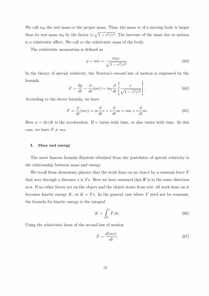
We call m0 the rest mass or the proper mass. Thus, the mass m of a moving body is larger

than its rest mass m0 by the factor 1/√

1− v2/c2. The increase of the mass due to motion

is a relativistic effect. We call m the relativistic mass of the body.

The relativistic momentum is defined as

p = mv =m0v√

1− v2/c2. (63)

In the theory of special relativity, the Newton’s second law of motion is expressed by the

formula

F =dp

dt=

d

dt(mv) = m0

d

dt

[v√

1− v2/c2

]. (64)

According to the above formula, we have

F =d

dt(mv) = m

d

dtv + v

d

dtm = ma + v

d

dtm. (65)

Here a = dv/dt is the acceleration. If v varies with time, m also varies with time. In this

case, we have F 6= ma.

I. Mass and energy

The most famous formula Einstein obtained from the postulates of special relativity is

the relationship between mass and energy.

We recall from elementary physics that the work done on an object by a constant force F

that acts through a distance s is Fs. Here we have assumed that F is in the same direction

as s. If no other forces act on the object and the object starts from rest, all work done on it

becomes kinetic energy K, so K = Fs. In the general case where F need not be constant,

the formula for kinetic energy is the integral

K =

∫ s

0

F ds. (66)

Using the relativistic form of the second law of motion

F =d(mv)

dt, (67)

18

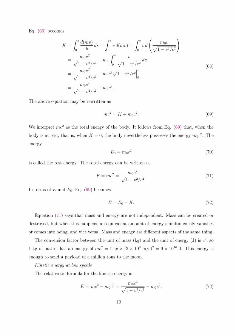
Eq. (66) becomes

K =

∫ s

0

d(mv)

dtds =

∫ v

0

v d(mv) =

∫ v

0

v d

(m0v√

1− v2/c2

)

=m0v

2

√1− v2/c2

−m0

∫ v

0

v√1− v2/c2

dv

=m0v

2

√1− v2/c2

+ m0c2√

1− v2/c2

∣∣∣v

0

=m0c

2

√1− v2/c2

−m0c2.

(68)

The above equation may be rewritten as

mc2 = K + m0c2. (69)

We interpret mc2 as the total energy of the body. It follows from Eq. (69) that, when the

body is at rest, that is, when K = 0, the body nevertheless possesses the energy m0c2. The

energy

E0 = m0c2 (70)

is called the rest energy. The total energy can be written as

E = mc2 =m0c

2

√1− v2/c2

. (71)

In terms of E and E0, Eq. (69) becomes

E = E0 + K. (72)

Equation (71) says that mass and energy are not independent. Mass can be created or

destroyed, but when this happens, an equivalent amount of energy simultaneously vanishes

or comes into being, and vice versa. Mass and energy are different aspects of the same thing.

The conversion factor between the unit of mass (kg) and the unit of energy (J) is c2, so

1 kg of matter has an energy of mc2 = 1 kg × (3 × 108 m/s)2 = 9 × 1016 J. This energy is

enough to send a payload of a million tons to the moon.

Kinetic energy at low speeds

The relativistic formula for the kinetic energy is

K = mc2 −m0c2 =

m0c2

√1− v2/c2

−m0c2. (73)

19

Consider the case where v ¿ c. We use the approximation (1 + x)n ∼= 1 + nx for small x to

expand the first term in the above formula. Then we obtain the expression

K = mc2 −m0c2 ∼= 1

2m0v

2, (74)

in agreement with classical mechanics.

Energy and momentum

Total energy and momentum are conserved in an isolated system, and the rest energy

of a particle is invariant. Hence these quantities are in some sense more fundamental than

kinetic energy and velocity. Let’s look into how the total energy, rest energy, and momentum

of a particle are related.

Total energy is

E =m0c

2

√1− v2/c2

. (75)

Square of E is

E2 =m2

0c4

1− v2/c2. (76)

Momentum is

p =m0v√

1− v2/c2. (77)

We have

p2c2 =m2

0v2c2

1− v2/c2. (78)

When we subtract p2c2 from E2, we obtain

E2 − p2c2 =m2

0c4 −m2

0v2c2

1− v2/c2= m2

0c4. (79)

Hence, we have the relation

E2 = m20c

4 + p2c2. (80)

Massless particles

In classical mechanics, a particle must have rest mass in order to have energy and mo-

mentum. However, this requirement does not hold true in relativistic mechanics.

When m0 = 0 and v < c, we find from Eqs. (75) and (77) that E = p = 0. Such a

particle is meaningless. However, when m0 = 0 and v = c, we have E = 0/0 and p = 0/0,

indicating that E and p can have any values. Thus, massless particles may exist if they

20

travel with the speed of light. The relation between the total energy E and the momentum

p of a massless particle is

E = pc. (81)

An example of massless particles is the photon.

J. Velocity addition

Special relativity postulates that the speed of light c in free space has the same value for

all observers, regardless of their relative motion. Common sense tells us that if we throw a

ball forward at 10 m/s from a car moving at 30 m/s, the ball’s speed relative to the road

will be 40 m/s. What if we switch on the car’s headlights when its speed is v? The same

reasoning suggests that their light ought to have a speed of c + v relative to the road. But

this violates the above postulate. Common sense is not reliable in dealing with light or with

a body moving with a speed comparable to the speed of light. To get the correct results for

velocity addition, we must use the Lorentz transformation.

Consider something moving relative to both S and S ′. An observer in S measures its

three velocity components to be

Vx =dx

dt, Vy =

dy

dt, Vz =

dz

dt. (82)

Meanwhile, to an observer in S ′ they are

V ′x =

dx′

dt′, V ′

y =dy′

dt′, V ′

z =dz′

dt′. (83)

By differentiating the Lorentz transformation equations for x′, y′, z′, and t′, we obtain

dx′ =dx− vdt√1− v2/c2

dy′ = dy

dz′ = dz

dt′ =dt− (v/c2)dx√

1− v2/c2.

(84)

21

So we have

V ′x =

dx′

dt′=

dx− vdt

dt− (v/c2)dx=

dxdt− v

1− (v/c2)dxdt

=Vx − v

1− (vVx/c2),

V ′y =

dy′

dt′=

dy√

1− v2/c2

dt− (v/c2)dx=

dydt

√1− v2/c2

1− (v/c2)dxdt

=Vy

√1− v2/c2

1− (vVx/c2),

V ′z =

dz′

dt′=

dz√

1− v2/c2

dt− (v/c2)dx=

dzdt

√1− v2/c2

1− (v/c2)dxdt

=Vz

√1− v2/c2

1− (vVx/c2).

(85)

Thus, the formulae for velocity addition are

V ′x =

Vx − v

1− (vVx/c2),

V ′y =

Vy

√1− v2/c2

1− (vVx/c2),

V ′z =

Vz

√1− v2/c2

1− (vVx/c2).

(86)

The inverse formulae are

Vx =V ′

x + v

1 + (vV ′x/c

2),

Vy =V ′

y

√1− v2/c2

1 + (vV ′x/c

2),

Vz =V ′

z

√1− v2/c2

1 + (vV ′x/c

2).

(87)

Consider a ray of light emitted in the moving frame S ′ in its direction of motion relative

to S. In this case, we have V ′x = c. An observer in S will measure the speed

Vx =V ′

x + v

1 + (vV ′x/c

2)=

c + v

1 + (vc/c2)= c. (88)

Thus both observers in S and S ′ find the same value for the speed of light.

Example

Spacecraft A is moving at a speed of 0.9c with respect to the earth. If spacecraft B is

to pass A at a relative speed of 0.5c in the same direction, what speed must B have with

respect to the earth.

Solution

Conventional mechanics says that the speed of B ought to be 1.4c, that is, larger than

the speed of light. However, according to the special relativity, the necessary speed of B is

only

Vx =V ′

x + v

1 + (vV ′x/c

2)=

0.5c + 0.9c

1 + (0.5c)(0.9c)/c2)= 0.97c. (89)

This speed is less than c.

22

II. WAVE PROPERTIES OF PARTICLES

A. De Broglie waves

A photon of light of frequency ν has the energy E = hν. According to the special relativity

theory, the energy E is related to the momentum p as E = pc. Hence, the momentum of a

photon is

p =hν

c. (90)

Here, h = 6.626 × 10−34 J s is the Planck’s constant and c = 2.998 × 108 m/s is the speed

of light in free space.

On the other hand, the wavelength of a photon is λ = c/ν. When we use Eq. (90), we

find the following relation between the wavelength and momentum of a photon:

λ =h

p. (91)

The momentum p describes the particle property of the photon. The wavelength λ de-

scribes the wave property of the photon. Each photon has both particle and wave properties.

De Broglie suggested that Eq. (91) is completely general: It applies not only to photons

but also to material particles. A material particle, i.e., a moving body, can behave as it

has a wave nature. The matter waves are called the de Broglie waves. The wavelength of

a particle is given by Eq. (91) and is called the de Broglie wavelength. The greater the

particle’s momentum, the shorter its de Broglie wavelength.

The momentum of a particle of mass m and velocity v is p = mv. The de Broglie

wavelength is therefore given by

λ =h

mv. (92)

In the above equation, m is the relativistic mass, which is related to the rest mass m0 as

m =m0√

1− v2/c2. (93)

The wave and particle properties of moving bodies can never be observed at the same time.

In some situations a moving body resembles a wave and in others it resembles a particle.

Which set of properties is most conspicuous depends on how its de Broglie wavelength

compares with its dimensions and the dimensions of whatever it interacts with.

To illustrate this statement, we show two examples.

23

Example 1

Find the de Broglie wavelength of a dust particle with a mass of 10−15 kg and a velocity

of 1 mm/s.

Solution

Since v ¿ c, we can let m = m0. Hence

λ =h

mv=

6.6× 10−34 J s

(10−15 kg)× (10−3 m/s)= 6.6× 10−16 m. (94)

Assume that the diameter of the dust particle is 1 µm. Then, the de Broglie wavelength

of the dust particle is very small compared with its dimensions. Therefore, we do not expect

to find any wave aspects in its behavior.

Example 2

Find the de Broglie wavelength of an electron with a velocity of 107 m/s. The rest mass

of an electron is m0 = 9.1× 10−31 kg.

Solution

Since v ¿ c, we can let m = m0. Hence

λ =h

mv=

6.6× 10−34 J s

(9.1× 10−31 kg)× (107 m/s)= 7.3× 10−11 m. (95)

The radius of the hydrogen atom is 5.3 × 10−11 m. The de Broglie wavelength of the

electron (with a velocity of 107 m/s) is comparable with the dimensions of atoms. Therefore,

the wave character of moving electrons is the key to understanding atomic structure and

behavior.

B. Wave function: de Broglie waves are waves of probability amplitude

In water waves, the quantity that varies periodically is the height of the water surface. In

sound waves, it is pressure. In light waves, electric and magnetic fields vary. What quantity

varies in the case of de Broglie matter waves?

The quantity whose variations make up matter waves is called the wave function and is

denoted by the symbol Ψ. This quantity is a function of space and time, i.e., Ψ = Ψ(r, t).

The value of the wave function Ψ at the particular point r = (x, y, z) in space at the time

t is related to the likelihood of finding the body there at the time. More precisely, |Ψ(r, t)|2,

24

the square of the absolute value of the wave function, is the probability of finding the body at

the point r at the time t. The value of the wave function Ψ(r, t) is the probability amplitude.

It can be negative, and is not an observable quantity.

C. Describing a wave

Consider a string stretched along the x direction. We shake the string at x = 0 up and

down along the y direction. Assume that the vibrations are harmonic in character. The

displacement of the string at x = 0 can be written as

y = A cos 2πνt. (96)

Here ν is the frequency of the vibrations and A is their amplitude.

A wave of vibrations propagates along the x direction with a wave velocity vp. Wave

formula:

y = A cos 2πν

(t− x

vp

). (97)

The wave velocity vp is called the phase velocity. Since the wave velocity vp is given by

vp = λν, we have

y = A cos 2π(νt− x

λ

). (98)

The angular frequency is defined by the formula

ω = 2πν. (99)

The wave number k is defined by the formula

k =2π

λ=

ω

vp

. (100)

In terms of ω and k, the wave formula can be written as

y = A cos(ωt− kx). (101)

In the three-dimensional space, k becomes a vector k normal to the wave fronts and x is

replaced by the radius vector r. Then, kx is replaced by the scalar product k · r = kr.

In the case of de Broglie waves, the momentum of the particle is

p = h/λ = hk/2π = hk. (102)

25

Here, h = h/2π = 1.054× 10−34 J s is the reduced Planck’s constant.

Exercise 1:

A photon and a particle have the same wavelength. (a) Compare their linear momenta.

(b) Compare the photon’s energy and the particle’s total energy. (c) Compare the photon’s

energy and the particle’s kinetic energy.

Answer:

(a) They have the same linear momenta: p = h/λ.

(b) The photon’s energy is Eph = hν = hc/λ = pc. The particle’s total energy is

Ep =√

p2c2 + E20 . Thus the photon’s energy is smaller than the particle’s total energy.

(c) The particle’s kinetic energy is K = Ep − E0 =√

p2c2 + E20 − E0 < pc. Thus the

particle’s kinetic energy is smaller than the photon’s energy.

Exercise 2:

Show that the de Broglie wavelength of a particle of rest mass m0 and kinetic energy K

is λ = hc/√

K(K + 2m0c2).

Answer: Be definition, we have λ = h/p = hc/pc. To calculate pc, we use the kinetic

energy K = E − E0 =√

p2c2 + E20 − E0 =

√p2c2 + m2

0c4 −m0c

2. The latter yields pc =√

K(K + 2m0c2). Hence, we obtain

λ = hc/√

K(K + 2m0c2). (103)

Note that, when v ¿ c, we have K = m0c2(1/

√1− v2/c2 − 1) ¿ m0c

2. Hence, we obtain

λ = h/√

2m0K. This formula can be derived by another way using the nonrelativistic

formulae λ = h/p and K = p2/2m0.

Exercise 3:

Show that if the total energy of a moving particle greatly exceeds its rest energy, its de

Broglie wavelength is nearly the same as the wavelength of a photon with the same total

energy.

Answer: For a particle, we have E =√

p2c2 + E20 . Hence, pc =

√E2 − E2

0 . When

E À E0, we obtain pc ∼= E. In this case, the de Broglie wavelength of the particle is

λp = h/p ∼= hc/E. Meanwhile, for a photon, we always have E = pc and hence, λph =

h/p = hc/E. Thus λp∼= λph.

26

D. Phase and group velocities of de Broglie waves

How fast do de Broglie waves travel? Since a de Broglie wave is associated with a moving

body, one may expect that this wave has the same velocity as that of the body. Let us see

if this is true.

We call the de Broglie wave velocity vp. To find vp, we can apply the usual formula

vp = νλ. (104)

The wavelength λ is simply the de Broglie wavelength, i.e.,

λ =h

mv. (105)

To find the frequency ν, we equate the quantum expression E = hν with the relativistic

expression E = mc2. Then we obtain

ν =mc2

h. (106)

The de Broglie wave velocity is therefore

vp = νλ =

(mc2

h

) (h

mv

)=

c2

v. (107)

The wave velocity vp is the phase velocity. The particle velocity v is the group velocity.

Because the particle velocity v must be less than the velocity of light c, the de Broglie wave

velocity is always larger than c. To understand this result, we must look into the distinction

between phase velocity and group velocity.

We consider a harmonic wave

y = A cos(ωt− kx). (108)

The de Broglie waves associated with a moving body cannot be represented simply by a for-

mula resembling Eq. (108). Instead, the wave representation of a moving body corresponds

to a wave packet, or wave group. A wave group is a superposition of individual waves of

different wavelengths. The interference of the individual waves with one another results in

the variation in amplitude that defines the group shape. If the velocities of the individual

waves are the same, the velocity of the wave group is the common phase velocity. However,

27

FIG. 6: A wave group.

if the phase velocity varies with wavelength, an effect called dispersion, the different indi-

vidual waves do not proceed together. As a result, the wave group has a velocity different

from the phase velocities of the individual waves. This is the case with de Broglie waves.

As an example, we consider the case where the wave group consists of two waves that

have the same amplitude A but differ by a small amount ∆ω in angular frequency and a

small amount ∆k in wave number:

y1 = A cos(ωt− kx),

y2 = A cos[(ω + ∆ω)t− (k + ∆k)x]. (109)

The wave group is then given by

y = y1 + y2

= 2A cos1

2(∆ω t−∆k x) cos

1

2[(2ω + ∆ω)t− (2k + ∆k)x]. (110)

Since ∆ω ¿ ω and ∆k ¿ k, we find

y = 2A cos1

2(∆ω t−∆k x) cos(ωt− kx). (111)

The above equation represents a wave of angular frequency ω and wave number k whose

amplitude is modulated by an angular frequency ∆ω/2 and a wave number ∆k/2.

The effect of the modulation is to produce successive wave groups. The phase velocity vp

is

vp =ω

k, (112)

and the velocity of the successive wave groups is

vg =∆ω

∆k. (113)

28

When ω and k have continuous spreads instead of the two values in the above discussion,

the group velocity is

vg =dω

dk. (114)

We now use Eqs. (112) and (114) to calculate the phase and group velocities of de Broglie

waves. The angular frequency of the de Broglie waves associated with a body of rest mass

m0 moving with the velocity v is

ω = 2πν =2πmc2

h=

2πm0c2

h√

1− v2/c2. (115)

The wave number of the de Broglie waves is

k =2π

λ=

2πmv

h=

2πm0v

h√

1− v2/c2. (116)

The group velocity of the de Broglie waves is

vg =dω

dk=

dω/dv

dk/dv. (117)

It follows from Eqs. (115) and (116) that

dω

dv=

2πm0v

h(1− v2/c2)3/2,

dk

dv=

2πm0

h(1− v2/c2)3/2. (118)

Hence, we find

vg = v. (119)

Thus, the group velocity of the de Broglie waves is the velocity of the moving body.

The phase velocity of the de Broglie waves is, as found earlier,

vp =ω

k=

c2

v. (120)

The fact that vp > c does not violate the special relativity theory because vp is the motion

of the phase of the wave group, not the motion of the individual waves that make up the

group, and consequently, not the motion of the body.

Exercise 1:

An electron has a de Broglie wavelength of 2× 10−12 m. Find its kinetic energy and the

phase and group velocities of its de Broglie waves.

29

Solution: First, we calculate pc:

pc =hc

λ=

(6.6× 10−34)(3× 108)

2× 10−12= 1× 10−13 J. (121)

The rest energy of the electron is E0 = m0c2 = (9.1× 10−31)(3× 108)2 = 0.8× 10−13 J. The

kinetic energy of the electron is

K = E − E0 =√

p2c2 + E20 − E0 =

√(1× 10−13)2 + (0.8× 10−13)2 − 0.8× 10−13

= 0.48× 10−13 J. (122)

In the units of eV (1 eV= 1.6× 10−19 J), we have K = 3× 105 eV = 300 keV.

To find the electron velocity v, we use the formula

v

c=

mcv

mc2=

pc

E=

pc√p2c2 + E2

0

=1× 10−13

√(1× 10−13)2 + (0.8× 10−13)2

= 0.78. (123)

Hence, the group velocity is vg = v = 0.78 c and the phase velocity is vp = c2/v = 1.28 c.

Exercise 2:

A proton and an electron have the same velocity. Compare the wavelengths and phase

and group velocities of their de Broglie waves.

Answer: (a) λ = h/p = h/mv. The electron has a smaller mass and consequently a longer

wavelength compared to those of the proton.

(b) Since vg = v, the de Broglie waves of the proton and electron have the same group

velocity.

(c) Since vp = c2/v, the de Broglie waves of the proton and electron have the same phase

velocity.

Exercise 3:

(a) A proton and an electron have the same kinetic energy. (b) Compare the wavelengths

and phase and group velocities of their de Broglie waves.

Answer: (a) λ = h/p and pc =√

K(K + 2m0c2) (or K ∼= p2/2m0 in nonrelativistic

considerations). The electron has a smaller mass than the proton. Therefore, we have

λelec > λproton.

(b) From K = E − E0 = m0c2(1/

√1− v2/c2 − 1), we find

v2

c2= 1−

(1− K

K + m0c2

)2

.

30

Since melec < mproton, we have velec > vproton. From the nonrelativistic formula K ∼= m0v2/2,

we get the same conclusion. Since vg = v and vp = c2/v, the electron has a larger group

velocity and a smaller phase velocity than the proton does.

Exercise 4:

Verify the statement that, if the phase velocity is the same for all wavelengths of a certain

wave phenomenon, the group and phase velocities are the same.

Answer: vp = ω/k and vg = dω/dk. If vp is a constant then vg = vp.

Exercise 5:

(a) Show that the phase group velocity of a particle of rest mass m0 and de Broglie

wavelength λ is vp = c√

1 + (m0cλ/h)2. (b) Compare the group and phase velocities of an

electron with the de Broglie wavelength of 1× 10−13 m.

Answer: (a) We have λ = h/p and p = m0v/√

1− v2/c2. Hence, we find

v = c/√

1 + (m0cλ/h)2. (124)

Since vg = v and vp = c2/v, we obtain

vp = c√

1 + (m0cλ/h)2. (125)

(b) For m0 = 9.1×10−31 kg, h = 6.6×10−34 Js, c = 3×108 m/s, λ = 1×10−13 m, we find

1 + (m0cλ/h)2 ∼= 1.0016. Consequently, vp/vg = 1.0016, vp∼= 1.0008 c and vg

∼= 0.9992 c.

31

FIG. 7: Scheme of the Davission-Germer experiment.

III. PARTICLE DIFFRACTION

A wave effect with no analog in the behavior of Newtonian particles is diffraction. In

1927, Davisson and Germer demonstrated that electron beams are diffracted when they are

scattered by the regular atomic arrays of crystal.

Davisson and Germer studied the scattering of electrons from a solid using an apparatus

sketched in Fig. 7. The energy of the electrons in the primary beam, the angle at which

they reach the target, and the position of the detector could all be varied.

Classical physics predicts that the scattered electrons will emerge in all directions with

only a moderate dependence of their intensity on scattering angle and even less on the energy

of the primary electrons. Using a block of nickel as the target, Davisson and Germer verified

these predictions. To prevent the crystal from being oxidized, the apparatus was kept in the

vacuum.

In the midst of their work an accident occurred that allowed air to enter their apparatus

and oxidize the metal surface. To reduce the oxide, the target was baked in a hot oven. After

this treatment, the target was returned to the apparatus and the measurements resumed.

Then the results were very different. Instead of a continuous variation of scattered electron

intensity with angle, distinct maxima and minima were observed whose positions depend on

the electron energy, see Fig. 8.

Two questions arise: What is the reason for this new effect? Why did it not appear until

the nickel target was baked?

De Broglie’s hypothesis suggested that electron waves were being diffracted by the target.

32

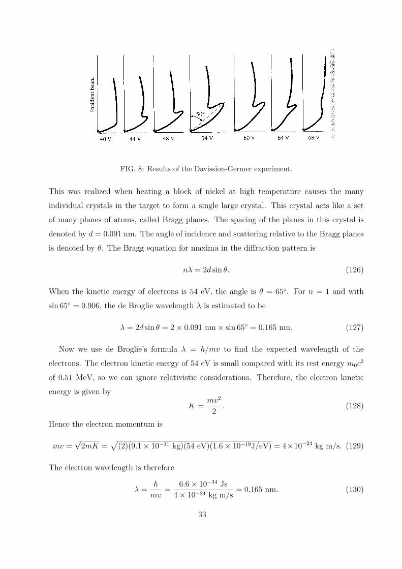
FIG. 8: Results of the Davission-Germer experiment.

This was realized when heating a block of nickel at high temperature causes the many

individual crystals in the target to form a single large crystal. This crystal acts like a set

of many planes of atoms, called Bragg planes. The spacing of the planes in this crystal is

denoted by d = 0.091 nm. The angle of incidence and scattering relative to the Bragg planes

is denoted by θ. The Bragg equation for maxima in the diffraction pattern is

nλ = 2d sin θ. (126)

When the kinetic energy of electrons is 54 eV, the angle is θ = 65◦. For n = 1 and with

sin 65◦ = 0.906, the de Broglie wavelength λ is estimated to be

λ = 2d sin θ = 2× 0.091 nm× sin 65◦ = 0.165 nm. (127)

Now we use de Broglie’s formula λ = h/mv to find the expected wavelength of the

electrons. The electron kinetic energy of 54 eV is small compared with its rest energy m0c2

of 0.51 MeV, so we can ignore relativistic considerations. Therefore, the electron kinetic

energy is given by

K =mv2

2. (128)

Hence the electron momentum is

mv =√

2mK =√

(2)(9.1× 10−31 kg)(54 eV)(1.6× 10−19J/eV) = 4×10−24 kg m/s. (129)

The electron wavelength is therefore

λ =h

mv=

6.6× 10−34 Js

4× 10−24 kg m/s= 0.165 nm. (130)

33

FIG. 9: The diffraction of the de Broglie waves by the target is responsible for the results of the

experiment.

Note that the realistic situation is more complicated than the above analysis. For ex-

ample, a complication arises from the fact that the energy of an electron increases when it

enters a crystal. Another complication is that there are several families of Bragg planes. The

interference between the waves diffracted from different families may prevent the observation

of maxima even when the Bragg condition is satisfied.

Exercise:

What effect on the scattering angle in the Davisson-Germer experiment does increasing

the electron energy have?

Answer: leads to a decrease of θ and an increase of the scattering angle ϕ.

Exercise:

A beam of 50-keV electrons is directed at a crystal and diffracted electrons are found at

an angle of 50◦ relative to the original beam. What is the spacing of the atomic planes of

the crystal? A relativistic calculation is needed for λ. Here m0c2 = 0.5 MeV.

Answer: We have

λ =hc√

K(K + 2m0c2)

=(6.6× 10−34 Js)(3× 108 m/s)

1.6× 10−19 J/eV√

(50× 103 eV)(50× 103 eV + 2(0.5× 106 eV))

=(6.6× 10−34)(3× 108)

1.6× 10−19 × [104 ×√

5× (5 + 100)]m =

19.8

1.6× 23× 10−11 m

= 0.5× 10−11 m = 0.005 nm. (131)

34

The spacing between the atomic planes is

d =λ

2 sin θ=

0.005 nm

2 sin 65◦=

0.005 nm

2× 0.906= 2.76× 10−3 nm. (132)

Exercise:

A beam of 5.4-keV electrons is directed at a crystal and diffracted electrons are found at

an angle of 50◦ relative to the original beam. What is the spacing of the atomic planes of

the crystal? We can ignore relativistic considerations.

Answer: We have

λ =h√

2m0K

=6.6× 10−34 Js√

(2)(9.1× 10−31 kg)(5.4× 103 eV)(1.6× 10−19 J/eV)

=6.6× 10−34 m√

15.7× 10−46=

6.6× 10−34 m

4× 10−23= 1.65× 10−11 m = 0.0165 nm. (133)

The spacing between the atomic planes is

d =λ

2 sin θ=

0.0165 nm

2 sin 65◦=

0.0165 nm

2× 0.906= 9.1× 10−3 nm. (134)

Particle in a box

The wave nature of a moving particle leads to some remarkable consequences when the

particle is restricted to a certain region of space instead of being able to move freely.

The simplest case is that of a particle in a box. We assume that the particle can move

only along one direction of the box, bouncing back and forth between the walls. We assume

that the walls are infinitely hard, so the particle does not lose energy each time it strikes a

wall. We also assume that the velocity of the particle is sufficiently small that we can ignore

relativistic considerations.

From a wave point of view, a particle trapped in a box is like a standing wave. The

possible de Broglie wavelengths of the particle are therefore determined by the width L of

the box. The longest wavelength is λ = 2L, the next is λ = L, then λ = 2L/3, and so forth.

The general formula is

λ =2L

n(n = 1, 2, 3, . . . ). (135)

Because mv = h/λ, the restrictions on λ imposed by the box width L are equivalent to

limits on the momentum of the particle and, in turn, to limits on its kinetic energy. The

35

kinetic energy of the particle is

K =mv2

2=

h2

2mλ2. (136)

Since the permitted wavelengths are λn = 2L/n and the particle has no potential energy in

this model, the permitted energies of the particle are

En =n2h2

8mL2(n = 1, 2, 3, . . . ). (137)

Each permitted energy is called an energy level. The integer number n that specified an

energy level En is called its quantum number.

We can draw three general conclusions:

1. A trapped particle cannot have an arbitrary energy, as a free particle can. The energies

are quantized (discrete) and can be characterized by a quantum number.

2. A trapped particle cannot have zero energy. The zero energy means v = 0 and

therefore λ = ∞. There is no way to trap a wave with an infinite wavelength in a box.

3. Because the Planck constant h is very small–only 6.63 × 10−34 J s – quantization of

energy is conspicuous only when m and L are also small. This is why we are not aware

of energy quantization in our own experience. The smaller the confinement, the larger the

energy required for confinement.

If a particle is confined into a rectangular volume (a three-dimentional box), the permitted

energies are

En1n2n3 =(n2

1 + n22 + n2

3)h2

8mL2(n = 1, 2, 3, . . . ). (138)

Exercise: The lowest possible energy of a particle in a box is 1 eV. What are the next

two higher energies the particle can have?

Answer: 4 eV and 9 eV.

36

FIG. 10: (a) A narrow de Broglie wave group. (b) A wide wave group.

IV. UNCERTAINTY PRINCIPLE

Look at the wave group of Fig. 6. The particle that corresponds to this wave group can

be found anywhere within the group at a given time. The probability of finding the particle

is given by |Ψ|2.When the wave group is narrower, the particle’s position can be specified more precisely,

see Fig. 10(a). However, the wavelength of the waves in a narrow packet is not well defined.

The reason is that the range of wavelengths of individual waves is large. This means that,

since λ = h/mv, the particle’s momentum is not a precise quantity. If we make a series of

momentum measurements, we will find a broad range of values.

When the wave group is wider, the particle’s wavelength can be specified more precisely,

see Fig. 10(b). Therefore, the momentum can be measured more precisely. However, since

the wave group is wide, the position of the particle is not well defined. If we make a series

of position measurements, we will find a broad range of values.

Thus we have the uncertainty principle (discovered by Heisenberg in 1927):

It is impossible to know both the exact position and exact momentum of an object at the

same time.

We present a mathematical expression for this principle. A moving body corresponds to

a single wave group, not a series of them. An isolated wave group is a superposition of an

infinite number of wave trains with different frequencies, wave numbers, and amplitudes, see

37

FIG. 11: An isolated wave group is the result of superposing an infinite number of waves with

different wave lengths.

Fig. 11.

At a certain time t, when Ψ(x) is a real function, the wave group Ψ(x) can be represented

by the Fourier integral

Ψ(x) =

∫ ∞

0

g(k) cos kx dk. (139)

More precisely and more generally, we have the formula

Ψ(x) =

∫ ∞

−∞g(k)eikx dk. (140)

The function g(k) describes the amplitudes and wavelengths of the harmonic waves that

contribute to the wave group. The narrower the wave group, the broader the range of

wavelengths involved, see Fig. 12.

We assume that the wave function Ψ(x) is spread in the interval ∆x, and that the

Fourier transform g(k) is spread in the interval ∆k. The spreads ∆x and ∆k are defined as

the standard deviations of x and k, respectively. These spreads are related to each other.

Due to the properties the Fourier transformation, we always have

∆x ∆k ≥ 1

2. (141)

To understand Eq. (141) qualitatively, we consider a simple example. Assume that

g(k) consists of only three individual components. The wave vectors of these individual

components are k0, k0−∆k/2, and k0 +∆k/2. Their amplitudes are proportional to 1, 1/2,

and 1/2, respectively. We then have

Ψ(x) = g0

{cos(k0x) +

1

2cos

[(k0 − ∆k

2

)x

]+

1

2cos

[(k0 +

∆k

2

)x

]}

= g0 cos(k0x)

[1 + cos

(∆k

2x

)]. (142)

38

FIG. 12: The wave functions and Fourier transforms for (a) a pulse, (b) a wave group, (c) a wave

train, and (d) a Gaussian distribution.

The above function is maximum at x = 0 and goes to zero at x = ±2π/∆k. The width of

this function is ∆x = 4π/∆k. Thus we have

∆x ∆k = 4π ≥ 1

2. (143)

If the wave function Ψ(x) is a Gaussian function, then the Fourier transform g(k) is also

a Gaussian function, and we have ∆x ∆k = 1/2. Indeed, we take

Ψ(x) = N exp

(− x2

4a2

). (144)

The width of Ψ(x) is ∆x = a. We find

g(k) = N ′ exp(−a2k2

), (145)

which is a Gaussian function. We can prove this with the help of the formula∫ ∞

−∞e−a2k2

cos kx dk =

√π

ae−

x2

4a2 . (146)

The width of g(k) is ∆k = 1/(2a). Thus we have ∆x ∆k = 1/2.

The Fourier transform g(k) is related to the probability of finding the particle with the

momentum p = hk. More precisely, |g(k)|2 is proportional to the probability for the particle

to have the momentum p = hk. When we use the relation ∆p = h∆k and Eq. (141), we

find

∆x ∆p ≥ h

2. (147)

The above equation is a mathematical expression of the uncertainty principle. The spreads

∆x and ∆k are the measures of the uncertainties in the position and momentum, respectively,

39

of the particle. Equation (147) says that the product of the uncertainty ∆x in the position

of an object at some instant and the uncertainty ∆p in its momentum component in the x

direction at the same time is equal or greater than h/2.

If we arrange the particle in such a way that ∆x is small, then ∆p will be large. If we

reduce ∆p in some way, then ∆x will be large.

Average value and standard deviation

Consider an observable A. Assume that the probability for A to take the value α is

described by the probability density ρ(α). The mean value of A is

〈A〉 =

∫ ∞

−∞αρ(α) dα. (148)

We introduce the notation

〈F (A)〉 =

∫ ∞

−∞F (α)ρ(α) dα. (149)

In particular, we have

〈An〉 =

∫ ∞

−∞αnρ(α) dα. (150)

The standard deviation ∆A of A is defined by the formula

(∆A)2 = 〈(A− 〈A〉)2〉 = 〈A2〉 − 〈A〉2. (151)

Compatible observables

If two observables A and B are compatible, they can be described by a joint probability

density ρ(α, β). We can define

〈F1(A)F2(B)〉 =

∫ ∞

−∞

∫ ∞

−∞F1(α)F2(β)ρ(α, β) dαdβ. (152)

Proof of the uncertainty principle

Consider the position x and the momentum p of a particle. In quantum mechanics, x

and p are not compatible, that is, the averages 〈xp〉 and 〈px〉 cannot be defined in the

conventional way. Moreover, we have

〈xp〉 6= 〈px〉. (153)

40

More precisely, we have

〈xp〉 − 〈px〉 = ih. (154)

Define δx = x− 〈x〉 and δp = p− 〈p〉. It follows from the above equation that

〈δxδp〉 − 〈δpδx〉 = ih. (155)

As known, CC∗ ≥ 0. For any real variable ξ, we always have

〈(δx + iξδp)(δx− iξδp)〉 ≥ 0. (156)

We calculate the left-hand side and find

〈(δx + iξδp)(δx− iξδp)〉 = aξ2 + bξ + c, (157)

where

a = 〈δp2〉b = −i(〈δxδp〉 − 〈δpδx〉)c = 〈δx2〉. (158)

Since aξ2 + bξ + c ≥ 0 for any real ξ, the following condition should be satisfied:

b2 ≤ 4ac. (159)

On the other hand, we have a = (∆p)2, b = h, and c = (∆x)2. Hence, we find

h2 ≤ 4(∆p)2(∆x)2, (160)

that is,

∆x∆p ≥ h

2. (161)

Uncertainty principle from the particle approach

Suppose we look at an electron using light of wavelength λ. Each photon of this light

has the momentum h/λ. We can see the electron only if one of these photons bounces off

the electron. The electron’s original momentum will be changed. The exact amount of the

41

change ∆p cannot be predicted but will be of the same order of magnitude as the photon

momentum h/λ. Consequently, the uncertainty in the electron’s momentum is

∆p ≈ h

λ. (162)

On the other hand, light is a wave phenomenon as well as a particle phenomenon. We

cannot determine the position of the electron with an accuracy better than the wavelength.

Consequently, we have

∆x ≥ λ. (163)

Combining Eqs. (162) and (163) gives

∆x∆p ≥ h. (164)

This result is consistent with the formula ∆x∆p ≥ h/2.

Uncertainty principle for energy and time

Another form of the uncertainty principle concerns energy and time.

Consider the measurement of the energy E emitted during the time interval ∆t in an

atomic process. Assume that the energy is in the form of electro-magnetic waves. The

energy is E = hν. Therefore, the uncertainty in energy is

∆E = h∆ν. (165)

To measure the frequency ν, we account the number of waves N for the interval ∆t and

divide this number by the time interval, that is, ν = N/∆t. Assume that the uncertainty in

number of waves in the wave group is one. Then, the uncertainty in frequency is

∆ν ≥ 1

∆t. (166)

It follows from Eqs. (165) and (166) that

∆E ∆t ≥ h. (167)

A more rigorous treatment gives

∆E ∆t ≥ h

2. (168)

42

Thus the product of the uncertainty in an energy measurement and the uncertainty in the

time at which the measurement is made is greater than or equal to h/2.

Consider a conservative system. For this system, the greater the energy uncertainty, the

more rapid the time evolution. More precisely, if ∆t is a time interval at the end of which

the system has evolved to an appreciable extent and if ∆E denotes the energy uncertainty,

∆t and ∆E satisfy the relation

∆E ∆t ≥ h

2. (169)

The above equation is a mathematical expression of the uncertainty principle for energy and

time.

The proof is given below. Consider a wave packet. The energy uncertainty ∆E is asso-

ciated with the momentum uncertainty ∆p via the formula

∆E =dE

dp∆p. (170)

Since E = hω and p = hk, we have

dE

dp=

dω

dk= vg. (171)

Hence

∆E = vg∆p. (172)

Now the characteristic evolution time ∆t is the time taken by this wave packet to pass a

point in space. If ∆x is the spatial extension of the wave packet, we have

∆t =∆x

vg

. (173)

From this we obtain

∆E∆t = ∆p∆x ≥ h

2. (174)

Example 1

A measurement establishes the position of a proton with an accuracy of ±1 × 10−11 m.

Find the uncertainty in the position of the proton 1 second later. The rest mass of a proton

is m0 = 1.672× 10−27 kg. Assume v ¿ c.

Solution

The uncertainty in the proton’s position at t = 0 is ∆x0 = 1 × 10−11 m. According to

Eq. (147), the uncertainty in its momentum at this time is

∆p ≥ h

2∆x0

. (175)

43

Since v ¿ c, the momentum is p = mv = m0v. Therefore, we have ∆p = m0∆v. Hence, the

uncertainty in the proton’s velocity is

∆v ≥ h

2m0∆x0

. (176)

After the time t, the position of the proton cannot be known more accurately than

∆x = t∆v ≥ ht

2m0∆x0

. (177)

Hence ∆x is inversely proportional to ∆x0. This means that the more we know about the

proton’s position at a given time, the less we know about its later position.

The value of ∆x at t = 1 s is

∆x ≥ (1.054× 10−34 J s)× (1 s)

2× (1.672× 10−27 kg)× (1× 10−11 m)= 3.15× 103 m. (178)

Exercise: (a) Discuss the prohibition of E = 0 for a trapped particle in a box in terms of

the uncertainty principle. (b) How does the minimum momentum of such a particle compare

with the momentum uncertainty required by the uncertainty principle if we take ∆x = L?

Answer: (a) Since the particle is trapped in the box, ∆x is not infinite. Therfore, ∆p

cannot be zero and consequently p cannot be zero. This is why the particle cannot have

E = 0. (b) If we take ∆x = L then ∆p ≥ h/2∆x = h/2L. On the other hand, the first

permitted value of λ is 2L. Therefore, the minimum momentum is pmin = h/λ = h/2L =

πh/L > h/2L. Thus the minimum momentum of the trapped particle is larger than the

momentum uncertainty required by the uncertainty principle.

Exercise: Compare the uncertainties in the velocities of an electron and a proton in a

small box.

Answer: Take ∆x = L. Then (∆p)min = h/2∆x = h/2L. Since p = mv, we have

(∆v)min = h/2mL. Hence, the uncertainty in the velocity of the electron is larger than that

of the proton.

Exercise: Verify that the uncertainty principle can be written as ∆L∆θ ≥ h/2, where L

is the angular momentum and θ is the angular position.

Answer: Consider the rotational motion of a particle along a circle of radius a. We

have L = mvr and θ = x/r. Hence ∆L = mr∆v = r∆p and ∆θ = ∆x/r. Therefore,

∆L∆θ = ∆p∆x ≥ h/2.

Exercise: A hydrogen atom is 5.3 × 10−11 m in radius. Use the uncertainty principle to

estimate the minimum kinetic energy an electron can have in this atom.

44

Answer: Here we have ∆x = 5.3× 10−11 m. The uncertainty in momentum is

∆p ≥ h

2∆x∼= 1× 10−24kgm/s. (179)

The momentum of the electron must be at least comparable to its uncertainty. Consequently,

the kinetic energy of the electron is

K =p2

2m≥ (1× 10−24)2

(2)(9.1× 10−31)J ≥ 5× 10−19 J ∼= 3 eV. (180)

45

V. ATOMIC SPECTRA

When an atomic gas is excited by passing an electric current through it, the emitted

radiation has a spectrum which contains specific wavelengths only.

Each element has a characteristic line spectrum.

The number, strength, and exact wavelengths of the lines in the spectrum of an element

depend on temperature, pressure, the presence of electric and magnetic fields, and the motion

of the source.

Spectroscopy is therefore a useful tool for analyzing the composition and the state of a

source.

A. Spectral series

It has been experimentally found that the spectral lines of an element fall into sets called

spectral series.

For hydrogen, the Lyman series contains the wavelengths given by the formula

1

λ= R

(1

12− 1

n2

)with n = 2, 3, 4, . . . , (181)

and is in the ultraviolet region (400–10 nm). Here, R = 1.097 × 107 m−1 is the Rydberg

constant.

The Balmer series contains the lines

1

λ= R

(1

22− 1

n2

)with n = 3, 4, 5, . . . , (182)

and is in the visible region (800–400 nm).

In the infrared region (from 800 nm to 1 mm), three series have been found. They are

Paschen:1

λ= R

(1

32− 1

n2

)with n = 4, 5, 6, . . . , (183)

Brackett:1

λ= R

(1

42− 1

n2

)with n = 5, 6, 7, . . . , (184)

and

Pfund:1

λ= R

(1

52− 1

n2

)with n = 6, 7, 8, . . . (185)

The existence of spectral lines and series poses a test for any theory of atomic structure.

46

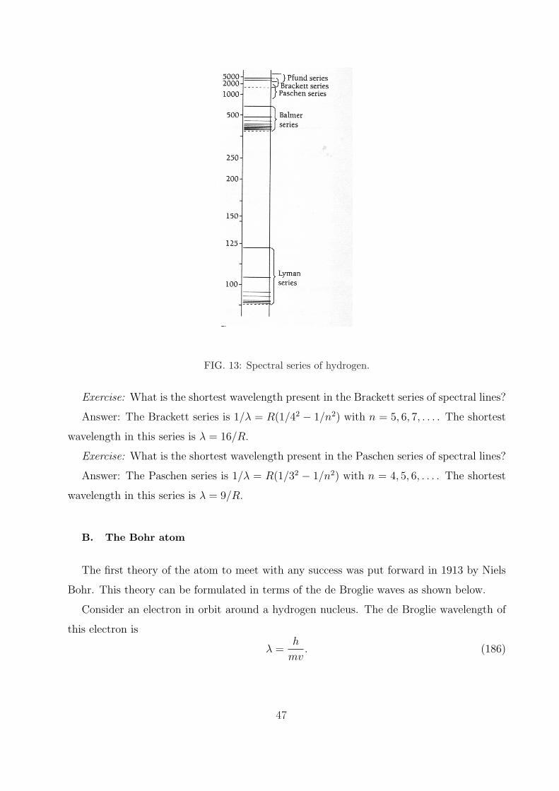
FIG. 13: Spectral series of hydrogen.

Exercise: What is the shortest wavelength present in the Brackett series of spectral lines?

Answer: The Brackett series is 1/λ = R(1/42 − 1/n2) with n = 5, 6, 7, . . . . The shortest

wavelength in this series is λ = 16/R.

Exercise: What is the shortest wavelength present in the Paschen series of spectral lines?

Answer: The Paschen series is 1/λ = R(1/32 − 1/n2) with n = 4, 5, 6, . . . . The shortest

wavelength in this series is λ = 9/R.

B. The Bohr atom

The first theory of the atom to meet with any success was put forward in 1913 by Niels

Bohr. This theory can be formulated in terms of the de Broglie waves as shown below.

Consider an electron in orbit around a hydrogen nucleus. The de Broglie wavelength of

this electron is

λ =h

mv. (186)

47

To determine v, we recall that the centripetal force is

Fc =mv2

r. (187)

This force is provided by the electric force

Fe =1

4πε0

e2

r2. (188)

The condition for a stable orbit is Fc = Fe, i.e.,

mv2

r=

1

4πε0

e2

r2. (189)

The electron velocity is therefore found to be

v =e√

4πε0mr. (190)

Hence, the orbital electron wavelength is

λ =h

e

√4πε0r

m. (191)

We assume that the motion of the electron in the hydrogen atom is analogous to the

vibrations of a wire loop. We know that, in a wire loop, the loop’s circumference is an

integer number of the wavelength of the resonant mode. Therefore, we assume that an

electron can circle a nucleus only if its orbit contains an integer number of the de Broglie

wavelength. Thus, the condition for orbital stability is

nλ = 2πr, with n = 1, 2, 3, . . . (192)

The integer n is called the quantum number of the orbit. When we substitute Eq. (192)

into Eq. (191), we find that the radii of the orbits are

r = rn = n2 h2ε0

πme2, with n = 1, 2, 3, . . . (193)

The radius of the innermost orbit is called the Bohr radius of the hydrogen atom and is

denoted by a0:

a0 = r1 =h2ε0

πme2= 5.292× 10−11 m. (194)

Here we have used the parameters e = 1.6×10−19 C, ε0 = 8.85×10−12 F/m, m0 = 9.1×10−31

kg, and h = 6.6× 10−34 Js.

48

FIG. 14: Vibrations of a wire loop.

The other radii are given in terms of a0 by the formula

rn = n2a0, with n = 1, 2, 3, . . . (195)

Exercise 1: In the Bohr model, the electron is in constant motion. How can such an

electron have a negative energy?

Answer: The potential energy of the electron interacting with the proton is U =

−e2/4πε0r, a negative value. The kinetic energy of the electron is K = mv2/2 = e2/8πε0r.

Since the absolute of the potential energy is larger than the kinetic energy, the total energy

E = K + U of the electron is negative.

Exercise 2: Derive a formula for the speed of an electron in the nth orbit of a hydrogen

atom using the Bohr model.

Answer: In the Bohr model, rn = n2a0, where a0 = h2ε0/πme2 is the Bohr radius. From

the condition for orbital stability nλ = 2πr, we have λ = 2πna0. From the de Broglie

relation λ = h/mv, we obtain v = h/nma0.

Exercise 3: An electron at rest is released far away from a proton and moves toward the

proton. (a) Show that the de Broglie wavelength λ is proportional to√

r, where r is the

distance of the electron from the proton. (b) Find λ when r = a0. How does this compare

with the wavelength of an electron in the ground-state Bohr orbit? (c) In order for the

electron to be captured by the proton to form a ground-state hydrogen atom, energy must

be lost by the system. How much energy?

Answer: (a) It follows from the energy conservation law E = K + U = 0 that K =

49

p2/2m = −U = e2/4πε0r. Hence p = e√

m/2πε0r. Therefore, λ = h/p =√

2πε0h2r/me2 =

π√

2a0r.

(b) When r = a0, we have λ = π√

2 a0. The wavelength of an electron in the ground-state

Bohr orbit is λ0 = 2πa0. As we can see, λ < λ0.

(c) The energy to be released is −E1 = −U/2 = (1/8πε0)(e2/r1) = e2/8πε0a0 =

me4/8ε20h

2 = 2.18× 10−18 J = 13.6 eV.

Exercise 4: Compare the uncertainty in the momentum of an electron confined to a region

of linear dimension a0 with the momentum of an electron in the ground-state Bohr orbit.

Answer: ∆p ≥ h/2a0. According to exercise 2, the momentum of an electron in the

ground-state Bohr orbit is p1 = mv1 = h/a0. Thus the uncertainty in the momentum of the

electron is less than the momentum of the electron in the ground-state Bohr orbit.

C. Energy levels and spectra

The total electron energy E is the sum of its kinetic energy

mv2

2(196)

and potential energy

− e2

4πε0r. (197)

This means that

E =mv2

2− e2

4πε0r. (198)

Due to Eq. (189), we find

E = − e2

8πε0r. (199)

Different permitted orbits have different energies: Due to Eq. (189), we find

En = − e2

8πε0rn

. (200)

When we use Eq. (193) for rn, we see that

En = − me4

8ε20h

2

1

n2=

E1

n2, with n = 1, 2, 3, . . . (201)

Here, E1 = −2.18× 10−18 J = −13.6 eV.

The energies specified by Eq. (201) are called the energy levels of the hydrogen atom.

These levels are all negative. This means that the electron does not have enough energy to

50

escape from the nucleus. An electron in the hydrogen atom can have only these energies

and no others.

The lowest level E1 is called the ground state, and the higher levels E2, E3, E4, . . . are

called excited states.

As the quantum number n increases, the level energy En tends to 0. In the limit of

n = ∞, we have E∞ = 0, that is, the electron is no longer bound to the nucleus to form an

atom. The work needed to remove an electron from its ground state is called its ionization

energy. It is equal to −E1. In the case of hydrogen, the ionization energy is 13.6 eV.

D. Origin of line spectra

According to the Bohr model, electrons cannot exist in an atom except in certain specific

energy levels. When an electron in an excited state drops to a lower state, the lost energy is

emitted as a single photon of light. If the energy of the initial state of the electron is Ei and

the energy of the final state of the electron is Ef , then the energy of the emitted photon is

hν = Ei − Ef . (202)

Here, ν is the frequency of the photon. According to Eq. (201), we have

Ei − Ef = E1

(1

n2i

− 1

n2f

), (203)

where ni is the quantum number of the initial state and nf is the quantum number of the

final state. Therefore, we have

ν = −E1

h

(1

n2f

− 1

n2i

). (204)

Since λ = c/ν, we find the formula for the spectrum:

1

λ= −E1

hc

(1

n2f

− 1

n2i

). (205)

The Lyman series corresponds to the case where nf = 1:

Lyman (nf = 1):1

λ= −E1

hc

(1

12− 1

n2

), with n = 2, 3, 4, . . . (206)

Balmer (nf = 2):1

λ= −E1

hc

(1

22− 1

n2

), with n = 3, 4, 5, . . . (207)

51

FIG. 15: Transitions between energy levels.

Paschen (nf = 3):1

λ= −E1

hc

(1

32− 1

n2

), with n = 4, 5, 6, . . . (208)

Brackett (nf = 4):1

λ= −E1

hc

(1

42− 1

n2

), with n = 5, 6, 7, . . . (209)

Pfund (nf = 5):1

λ= −E1

hc

(1

52− 1

n2

), with n = 6, 7, 8, . . . (210)

The Rydberg constant is calculated to be

R = −E1

hc=

me4

8ε20h

3c= 1.097× 107 m−1. (211)

Thus, the theoretical results of the Bohr model are in agreement with the experimental

results.

Example 1

Find the longest wavelength present in the Balmer series of hydrogen.

Solution

In the Balmer series, the quantum number of the final state is nf = 2. The wavelengths

of the lines in this series is given by the formula

1

λ= R

(1

22− 1

n2

), with n = 3, 4, 5, . . . (212)

52

The longest wavelength corresponds to n = 3:

1

λ= R

(1

22− 1

32

)= 0.139 R. (213)

Hence, we obtain

λ =1

0.139 R=

1

0.139× (1.097× 107 m−1)= 6.56× 10−7 m = 656 nm. (214)

Exercise 1: When radiation with a continuous spectrum is passed through a volume of

hydrogen gas whose atoms are all in the ground state, which spectral series will be present

in the resulting absorption spectrum?

Answer: Lyman series: 1/λ = R(1− 1/n2).

Exercise 2: A proton and an electron, both at rest initially, combine to form a ground-

state hydrogen atom. A single photon is emitted in this process. What is its wavelength?

Answer: The energy of the ground state is E1. The wavelength of the emitted photon is

1/λ = −E1/ch = R = 1.097× 107 m−1. Hence λ = 0.912× 10−7 m = 91.2 nm.

Exercise 3: How many different wavelengths would appear in the emission spectrum of

hydrogen atoms initially in the n = 5 state?

Answer: 4 lines (n = 5 → n′ = 1, 2, 3, 4) for the downward transitions with ni = 5.

However, there are 10 lines for the downward transitions with ni = 5, 4, 3, 2.

Exercise 4: An excited hydrogen atom emits a photon in returning to the ground state.

Derive a formula for the quantum number ni of the initial state in terms of λ and R. Use

this formula to find ni for a 102.55-nm photon.

Answer: Lyman series: 1/λ = R(1 − 1/n2). Hence we find n = 1/√

1− 1/λR.

For a 102.55-nm photon, we find n = 1/√

1− 1/[(102.55× 10−9)(1.097× 107)] ==

1/√

1− 1/1.125 = 1/√

1− 0.889 = 1/√

0.111 = 1/0.333 = 3.

Exercise 5: Doppler effect An excited atom of mass m and initial speed v emits a photon

in its direction of motion. Assume that v is small compared to c, so that relativistic con-

siderations are not required. If hω/2mc2 ¿ 1, use the requirement that linear momentum

and energy must both be conserved to show that the frequency of the photon is higher by

∆ω/ω0∼= v/c than it would have been if the atom had been at rest.

Answer: We have two equations

mv = hk + mv′,

Ei +mv2

2= Ef + hω +

mv′2

2. (215)

53

Introduce the notation Ei−Ef = hω0. Elimination of v′ from the above two equations gives

hω0 = hω

(1− v

c+

hω

2mc2

). (216)

Since hω/2mc2 ¿ 1, we neglect this term. Consequently, we obtain

ω =ω0

1− v/c∼= ω0(1 + v/c). (217)

Then, we have ∆ω/ω ∼= v/c.

54

VI. CORRESPONDENCE PRINCIPLE

Quantum physics is very different from classical physics in the microworld. However,

quantum physics must give the same results as classical physics in the macroworld where

classical physics is valid. We show that this basic requirement is true for the Bohr model of

the hydrogen atom.

We calculate the frequency of radiation from a hydrogen atom.

a) Classical picture. According to the electromagnetic theory, the radiation frequency of

a hydrogen atom is equal to the frequency of the evolution of the electron rotating around

the nucleus, or to an integer multiple of this frequency. According to Eq. (190), the speed

of the electron is

v =e√

4πε0mr. (218)

Hence, the evolution frequency of the electron is

f =v

2πr=

e

2π√

4πε0mr3. (219)

The radius of an stable orbit is given in terms of the quantum number n by Eq. (193) as

r = n2 h2ε0

πme2. (220)

Therefore, the evolution frequency of the electron is

f =me4

4ε20h

3n3= −E1

h

2

n3. (221)

b) Quantum picture. According to the Bohr model, when the electron drops from an

orbit ni to an orbit nf , a photon is emitted. The frequency of the emitted photon is given

by Eq. (204) as

ν = −E1

h

(1

n2f

− 1

n2i

). (222)

Under what circumstances should the Bohr atom behave classically. Assume that the

electron orbit is so large that we might be able to measure it directly. In this case, quantum

effects ought to be negligible. An orbit 10 µm across, for instance, meets this specification.

The quantum number of this orbit is n = 435, a large number.

Let’s write n = ni and n− p = nf . With this notation,

ν = −E1

h

(1

(n− p)2− 1

n2

)= −E1

h

2np− p2

n2(n− p)2. (223)

55

When n is much larger than p, we can use the approximations 2np−p2 ≈ 2np and (n−p)2 ≈n2. Hence, we find the photon frequency

ν = −E1

h

2p

n3. (224)

When p = 1, the photon frequency ν is exactly the same as the frequency of rotation f of

the orbital electron given by Eq. (221). Multiples of the rotation frequency f are radiated

when p = 2, 3, 4, . . . . Hence, both quantum and classical pictures of the hydrogen atom give

the same results in the limit of very large quantum numbers.

The requirement that quantum physics give the same results as classical physics in the

limit of large quantum numbers was called by Bohr the correspondence principle.

Since the de Broglie electron wavelength is λ = h/mv, we can rewrite the condition for

orbital stability nλ = 2πr, see Eq. (192), in the form

mvr =nh

2π. (225)

Exercise 1: Of the following quantities, which increase and which decrease in the Bohr

model as n increases: Frequency of evolution, electron speed, electron wavelength, angular

momentum, potential energy, kinetic energy, total energy.

Answer: Frequency of evolution f ∝ v/r ∝ 1/n3 decreases, electron speed v ∝ 1/√

r ∝1/n decreases, electron wavelength λ ∝ r/n ∝ n increases, kinetic energy K ∝ v2 ∝ 1/n2

decreases, potential energy U ∝ −1/r ∝ −1/n2 increases, total energy E ∝ −1/n2 increases.

Exercise 2: Show that the frequency of the photon emitted by a hydrogen atom in going

from the level n+1 to the level n is always intermediate between the frequencies of evolution

of the electron in the respective orbits.

Answer: Photon frequency is

ν =E1

h

[1

(n + 1)2− 1

n2

]=|E1|h

[1

n2− 1

(n + 1)2

]. (226)

The frequencies of revolution is

fn = −E1

h

2

n3=|E1|h

2

n3. (227)

Since2

(n + 1)3<

1

n2− 1

(n + 1)2<

2

n3, (228)

we have fn+1 < ν < fn.

56

FIG. 16: Transitions between two energy levels in an atom.

VII. THE LASERS

The laser is a device that produces a light beam with some remarkable properties:

1. The light is nearly monochromatic.

2. The light is coherent, with the waves all exactly in phase with each another. An

interference pattern can be obtained not only by placing two slits in a laser beam but also

by using beams from two separate lasers.

3. The beam is well collimated. It spreads out very little, even over long distances.

4. The beam is extremely intense, much more intense than any other source.

The key to the laser is the presence in many atoms of one or more excited energy levels

whose lifetimes may be 10−3 s or more instead of the usual 10−8 s. Such long-lived states

are called metastable (temporally stable).

Consider two energy levels E0 and E1. There are three kinds of transition involving these

levels. If the atom is initially in the lower state E0, it can be raised to E1 by absorbing a

photon of energy E1 − E0 = hν. This process is called induced absorption. If the atom is

initially in the upper state E1, the atom can drop to E0 by emitting a photon of energy hν.

This process is called spontaneous emission.

Einstein in 1917 pointed out that there is a third possibility, called induced emission,

in which an incident photon of energy hν causes a transition from E1 to E0. In induced

emission, the radiated light waves are exactly in phase with the incident ones, so the result is

an enhanced beam of coherent light. Induced emission has the same probability as induced

absorption. In other words, when a photon is incident to an atomic system, the probability

of emission of an initially excited atom is equal to the probability of absorption of an initially

unexcited atom.

A three-level laser

57

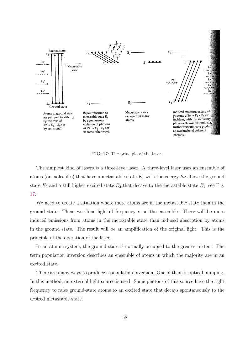
photons

FIG. 17: The principle of the laser.

The simplest kind of lasers is a three-level laser. A three-level laser uses an ensemble of

atoms (or molecules) that have a metastable state E1 with the energy hν above the ground

state E0 and a still higher excited state E2 that decays to the metastable state E1, see Fig.

17.

We need to create a situation where more atoms are in the metastable state than in the

ground state. Then, we shine light of frequency ν on the ensemble. There will be more

induced emissions from atoms in the metastable state than induced absorption by atoms

in the ground state. The result will be an amplification of the original light. This is the

principle of the operation of the laser.

In an atomic system, the ground state is normally occupied to the greatest extent. The

term population inversion describes an ensemble of atoms in which the majority are in an

excited state.

There are many ways to produce a population inversion. One of them is optical pumping.

In this method, an external light source is used. Some photons of this source have the right

frequency to raise ground-state atoms to an excited state that decays spontaneously to the

desired metastable state.

58

FIG. 18: The ruby laser.

Why are three levels needed? Suppose that there are only two levels. The pumping will

produce not only upward but also downward transitions. When half of the atoms are in

each state, the rate of induced emission is equal to the rate of induced absorption, so the

atomic ensemble cannot ever have more than half its atoms in the metastable state. Due to

the lack of population inversion, laser amplification cannot occur.

A practical three-level laser

The first successful laser is the ruby laser. It is based on the three energy levels in the

chromium ion Cr3+. A ruby is a crystal of aluminum oxide, Al2O3, in which some of the Al3+

ions are replaced by Cr3+ ions. A Cr3+ ion has a metastable level whose lifetime is about

0.003 s. In the ruby laser, a xenon flash lamp excites the Cr3+ ions to a higher level from

which they fall to the metastable level by losing energy to other ions in the crystal. Photons

from the spontaneous emission of some Cr3+ ions are reflected back and forth between two

mirrors at the ends of the ruby rod, stimulating other excited Cr3+ ions to radiate. After a

few microseconds, the result is a large pulse of monochromatic, coherent red light from the

partly transparent end of the rod.

The length of the rod is made to be an integer multiple of half-wavelength, so the radiation

trapped in its forms an optical standing wave. Since the induced emissions are stimulated

by the standing wave, the generated waves are all in phase with it.

Exercise 1: For laser action to occur, the medium used must have at least three energy

levels. What must be the nature of each of these levels? Why is three the minimum number?

Answer: One level is the ground state, another one is an excited state, the last one is an

metastable (long-lived) state.

If there is only two levels, one cannot achieve positive population inversion. Optical

pumping produces not only upward but also downward transitions. Therefore, in a two-

59

level system, the population of the upper level cannot be larger than the population of the

lower level.

Exercise 2: A ruby laser emits 1-J pulses of light whose wavelength is 694 nm. What is

the minimum number of Cr3+ ions in the ruby?

Answer: The energy of a photon is hω = hc/λ = (6.63× 10−34)(3× 108)/(694× 10−9) =

2.87× 10−19 J. The number of photons in each pulse is N = 1/(2.87× 10−19) = 3.5× 1018.

This is the minimum number of Cr3+ ions required for such laser pulses.

60

VIII. QUANTUM MECHANICS

The fundamental difference between classical (or Newtonian) and quantum mechanics

lies in what they describe.

In classical mechanics, the future history of a particle is completely determined by its

initial position and momentum together with the forces that act on it. In the everyday

world, i.e. the world of macroscopic bodies, all these quantities can be determined well

enough for the predictions of classical mechanics to agree with observations.

The uncertainty principle suggests that the nature of an observable quantity is different

in the world of microscopic particles. It is impossible to determine exactly the future history

of a particle because its initial state cannot be established with sufficient accuracy. This

world requires quantum mechanics.

The quantities whose relationships quantum mechanics explores are probabilities. For

example, instead of asserting that the radius of the electron’s orbit in the ground-state

hydrogen atom is 5.3 × 10−11 m, as the Bohr theory does, quantum mechanics states that

this is the most probable radius. In a suitable experiment most trials will yield different

values, either larger or smaller, the value most likely to be found will be 5.3× 10−11 m.

Classical mechanics is an approximate version of quantum mechanics. The certainties

in classical mechanics are illusory, and their apparent agreement with experiment occurs

because ordinary objects consist of so many individual atoms that departures from average

behavior are unnoticeable.

Wave function

The quantity with which quantum mechanics is concerned is the wave function Ψ of a

body. The wave function Ψ itself has no physical interpretation. However, the square of its

absolute value, |Ψ(x, t)|2, evaluated at a particular place x at a given time t, is proportional

to the probability of finding the body there at that time. The probabilities of all other

characteristics of the body, such as linear momentum, angular momentum, and energy, can

also be established from Ψ.

The problem of quantum mechanics is to determine Ψ for a body when its freedom of

motion is limited by the action of external forces.

Wave functions are usually complex, with both real and imaginary parts. Every complex

61

wave function can be written as

Ψ = A + iB, (229)

where A and B are real functions.

The complex conjugate is

Ψ∗ = A− iB. (230)

The probability density is

|Ψ|2 = ΨΨ∗ = A2 + B2. (231)

Thus the probability density P ∝ |Ψ|2 is always a positive real number, as required.

We now establish certain requirements for Ψ.

Since |Ψ|2 is proportional to the probability of finding the body at a point, the integral

of |Ψ|2 over all space, ∫ ∞

−∞|Ψ|2dV (232)

is proportional to the probability of finding the body somewhere in space. Therefore, this

integral must be finite. It cannot be 0 or ∞. If this integral is zero, the particle does not

exist. If this integral is ∞, it cannot not have the meaning of a probability.

It is convenient to have |Ψ|2 be equal to the probability density P of finding the particle.

If so, then it must be true that ∫ ∞

−∞|Ψ|2dV = 1 (233)

because ∫ ∞

−∞PdV = 1 (234)

A wave function that satisfies Eq. (234) is said to be normalized. Every acceptable wave

function can be normalized by multiplying it by an appropriate constant.

Besides being normalizable, Ψ must be single-valued since P can have only one value at

a particular place and time. Ψ must also be continuous. On the other hand, the momentum

components are proportional to the partial derivatives ∂Ψ/∂x, ∂Ψ/∂y, ∂Ψ/∂z. Therefore,

these derivatives must be finite, continuous, and single-valued. Only wave functions with

all these properties can yield physically meaningful results when used in calculations, so

only such well-behaved wave functions are admissible as mathematical representations of

real bodies.

To summarize:

62

1. Ψ must be single-valued and continuous everywhere.

2. ∂Ψ/∂x, ∂Ψ/∂y, ∂Ψ/∂z must be single-valued and continuous everywhere.

3. Ψ must be normalizable, which means that Ψ must go to 0 as x, y, or z tends to ±∞in order that

∫ |Ψ|2dV over all space be a finite constant.

The above rules are not always obeyed by the wave functions of particles in model situ-

ations that only approximate actual ones.

Exercise: Which of the wave functions in Fig. 5.14 of the textbook cannot have physical

significance in the interval shown? Why not?

Answer: (b), not single-valued; (c), derivative not continuous; (d), derivative not finite

and not continuous; (f), not continuous.

63

IX. SCHRODINGER EQUATION

Wave equation

Consider a wave whose variable quantity is y. Assume that this wave propagates in the

x direction with the speed v. Then, the propagation of the wave is described by the wave

equation∂2y

∂x2=

1

v2

∂2y

∂t2. (235)

All the solutions of the above equation must be of the form

y = F(t± x

v

), (236)

where F is any function that can be differentiated. The solutions F (t−x/v) represent waves

traveling in the +x direction, and the solutions F (t + x/v) represent waves traveling in the

−x direction.

Consider the wave equivalent of a free particle moving in the +x direction. This wave is

described as an undamped, monochromatic harmonic wave

y = Ae−iω(t−x/v). (237)

Time-dependent Schrodinger equation

In quantum mechanics, a particle is described by a wave function Ψ. We assume that

the wave function of a free particle moving along the +x direction is specified by

Ψ = Ae−iω(t−x/v). (238)

When we use the relations ω = 2πν and v = λν, we have

Ψ = Ae−2πi(νt−x/λ). (239)

In terms of the total energy E = hν = 2πhν and the momentum p = h/λ = 2πh/λ, the

wave function of the free particle is

Ψ = Ae−(i/h)(Et−px). (240)

We differentiate Eq. (240) twice with respect to x. Then we obtain

∂2Ψ

∂x2= −p2

h2 Ψ. (241)

64

Differentiating Eq. (240) once with respect to t gives

∂Ψ

∂t= − iE

hΨ. (242)

Assume that Eqs. (241) and (242) are valid for an arbitrary particle. Assume that the

velocity v of the particle is small compared to the light velocity c. Then, the total energy

E of the particle is the sum of its kinetic energy p2/2m and its potential energy U(x, t):

E =p2

2m+ U(x, t). (243)

Substituting Eq. (243) into Eq. (242) and using Eq. (241), we obtain the equation

ih∂Ψ

∂t= − h2

2m

∂2Ψ

∂x2+ UΨ. (244)

This is the time-dependent Schrodinger equation in one dimension.

In three dimensions, the time-dependent Schrodinger equation is

ih∂Ψ

∂t= − h2

2m

(∂2Ψ

∂x2+

∂2Ψ

∂y2+

∂2Ψ

∂z2

)+ UΨ. (245)

Here, the potential energy U is a function of x, y, z, and t.

The Schrodinger equation is a basic principle. It must be postulated. It cannot be derived

from other principles of physics.

Linearity and superposition

An important property of the Schrodinger equation is that it is linear in the wave function

Ψ. This means that the equation has terms that contain Ψ and its derivatives but no terms

independent of Ψ and no terms that involve higher powers of Ψ and its derivatives.

As a result, a linear combination of solutions of the Schrodinger equation is also itself a

solution. If Ψ1 and Ψ2 are two solutions, then

Ψ = a1Ψ1 + a2Ψ2 (246)

is also a solution. Here, a1 and a2 are constants. Thus the wave functions Ψ1 and Ψ2 obey

the superposition principle that other waves do. Consequently, interference efects can occur

for wave functions just as they can for light, sound, water, and electromagnetic waves.

Exercise: Prove that the Schrodinger equation is linear by showing that

Ψ = a1Ψ1 + a2Ψ2 (247)

65

is also a solution of Eq. (244) if Ψ1 and Ψ2 are themselves solutions.

Expectation values

The wave function of a particle contains all the information about the particle. How to

extract information from the wave function? As an example, let us calculate the expectation

value 〈x〉 of the position of a particle that is described by the wave function Ψ(x, t) in one

dimension.

To make the procedure clear, we first consider a number of identical particles. Assume

that there are N1 particles at x1, N2 particles at x2, and so on. The average position is then

given by

x =N1x1 + N2x2 + N3x3 + · · ·

N1 + N2 + N3 + · · · =

∑Nixi∑Ni

. (248)

When we are dealing with a single particle, we must replace the number Ni of particles at

xi by the probability Pi that the particle be found in an interval dx at xi. This probability

is

Pi = |Ψi|2dx, (249)

where Ψi is the wave function evaluated at x = xi. Making the substitution Ni = Pi =

|Ψi|2dx and changing the summations to integrals, we find that the expectation value of the

position of the single particle is

〈x〉 =

∫∞−∞ x|Ψ|2dx∫∞−∞ |Ψ|2dx

. (250)

We say that Ψ is a normalized wave function if∫∞−∞ |Ψ|2dx = 1. When Ψ is normalized, the

expectation value for position is

〈x〉 =

∫ ∞

−∞x|Ψ|2dx. (251)

In more general, consider an arbitrary quantity G(x) that depends on the position x but

not on the momentum p. The expectation value of this quantity is calculated as

〈G(x)〉 =

∫ ∞

−∞G(x)|Ψ|2dx. (252)

The expectation value 〈p〉 for momentum cannot be calculated this way because, accord-

ing to the uncertainty principle, no such function as p(x) can exist. Indeed, if we specify x,

so that ∆x = 0, we cannot specify a corresponding p since ∆x∆p ≥ h/2. The same problem

occurs for the expectation value 〈E〉 for energy.

66

Example

A particle limited to the x axis has the wave function Ψ = ax between x = 0 and x = 1;

Ψ = 0 elsewhere.

(a) Find a for which Ψ is a normalized wave function.

(b) Find the probability that the particle can be found between x = 0.45 and x = 0.55.

(c) Find the expectation value 〈x〉 of the particle’s position.

Solution

(a) The constant a satisfies the normalization condition

1 =

∫ 1

0

|Ψ|2dx = a2

∫ 1

0

x2dx = a2x3

3

∣∣∣∣∣

1

0

=a2

3. (253)

Hence we find a =√

3.

(b) The probability is

∫ x2

x1

|Ψ|2dx = a2

∫ 0.55

0.45

x2dx = a2x3

3

∣∣∣∣∣

0.55

0.45

= 0.0251a2 = 0.0753. (254)

(c) The expectation value for position is

∫ 1

0

x|Ψ|2dx = a2

∫ 1

0

x3dx = a2x4

4

∣∣∣∣∣

1

0

=a2

4=

3

4. (255)

Steady-state Schrodinger equation

Note that the wave function of a free particle (U = 0) can be written as

Ψ = Ae−(i/h)(Et−px) = Ae−iEt/heipx/h = ψe−iEt/h, (256)

where ψ depends on position but not on time.

Consider the case where the particle is not free. Assume that the potential U is a function

of x but is independent of time. Consider the situation where the wave function Ψ can be

written in the form

Ψ = ψe−iEt/h, (257)

where ψ is independent of time. This situation is called the steady state. Substituting Eq.

(257) into Eq. (244), we find

Eψe−iEt/h = − h2

2me−iEt/h ∂2ψ

∂x2+ Uψe−iEt/h. (258)

67

Dividing the above equation by the common exponential factor gives

∂2ψ

∂x2+

2m

h2 (E − U)ψ = 0. (259)

The above equation is called the steady-state Schrodinger equation in one dimension. In

three dimensions, the steady-state Schrodinger equation is

∂2ψ

∂x2+

∂2ψ

∂y2+

∂2ψ

∂z2+

2m

h2 (E − U)ψ = 0. (260)

An important property of the steady-state Schrodinger equation is that, if it has one or

more solutions for a given system, each of these solutions corresponds to a specific value of

the energy E. That is how energy quantization appears in quantum mechanics.

Eigenvalues and eigenfunctions

The values of energy En for which the steady-state Schrodinger equation can be solved

are called eigenvalues or eigenenergies. The corresponding wave functions ψn are called

eigenfunctions or eigenstates. An example of a set of eigenenergies is the discrete energy

levels of the hydrogen atom:

En = − me4

32π2ε20h

2

1

n2, with n = 1, 2, 3, . . . (261)

68

FIG. 19: An infinite potential.

X. PARTICLE IN A BOX

The simplest quantum-mechanical problem is that of a particle trapped in a box with

infinitely hard walls. Consider a particle that is restricted to traveling along the x axis

between x = 0 and x = L by infinitely hard walls. This situation can be described by the

potential energy U that is infinite on both sides of the box and is a finite constant on the

inside. Because the particle cannot have an infinite amount of energy, it cannot exist outside

the box. Hence, the wave function ψ is zero for x ≤ 0 and x ≥ L. We will calculate the

steady-state wave function ψ for the inside of the box.

Inside the box, U is a constant. For convenience, we take U = 0 for the inside of the box.

Then, the steady-state Schrodinger equation (259) becomes

d2ψ

dx2+

2m

h2 Eψ = 0. (262)

The total energy E = K +U = K is positive because so is the kinetic energy K. The general

solution of the above equation is

ψ = A sin

√2mE

hx + B cos

√2mE

hx. (263)

Here, A and B are coefficients to be evaluated.

The boundary conditions are ψ(0) = 0 and ψ(L) = 0. From ψ(0) = 0, sin 0 = 0 and

cos 0 = 1, we find B = 0. The condition ψ(L) = 0 will be satisfied if sin√

2mEL/h = 0,

that is, if √2mE

hL = nπ, with n = 1, 2, 3, . . . . (264)

Hence, the energy of the particle can have only certain values

En =n2π2h2

2mL2, with n = 1, 2, 3, . . . . (265)

69

The above values are the eigenenergies of the particle. They constitute the energy levels of

the particle.

Wave function of a particle in a box

Since B = 0, the wave function of the particle inside a box is

ψn = A sin

√2mEn

hx. (266)

Using Eq. (265) for En, we find

ψn = A sinnπx

L. (267)

It is easy to verify that the above wave function satisfies the steady-state Schrodinger equa-

tion and the boundary conditions ψ(0) = ψ(L) = 0. Note that Eq. (267) is valid only for

0 ≤ x ≤ L. Outside the box, we have ψn = 0. We also note that the spatial derivative ψ′n of

the wave function (267) is not continuous at x = 0 as well as at x = L. The reason is that

the box with infinitely hard walls is just an approximate model, not a realistic situation (see

the next section).

To find the constant A, we calculate the integral of |ψn|2 from x = −∞ to x = +∞. We

find

∫ +∞

−∞|ψn|2dx =

∫ L

0

|ψn|2dx = A2

∫ L

0

sin2 nπx

Ldx =

A2

2

∫ L

0

(1− cos

2nπx

L

)dx

=A2L

2. (268)

To satisfy the normalization condition

∫ +∞

−∞|ψn|2dx = 1, (269)

we choose

A =

√2

L. (270)

Thus the normalized wave functions of the particle are

ψn =

√2

Lsin

nπx

L, with n = 1, 2, 3, . . . . (271)

The normalized wave functions ψ1, ψ2, and ψ3 together with the probability densities

|ψ1|2, |ψ2|2, and |ψ3|2 are plotted in Fig. 20.

As seen, ψn = 0 at x = 0 and x = L. At a particular place in the box, the probability

of finding the particle may be very different for different quantum numbers. For example,

70

FIG. 20: Wave functions and probability densities of a particle in a box with rigid walls.

|ψ1|2 has its maximum value in the middle of the box, while |ψ2|2 = 0 there. In other words,

a particle in the lowest energy level of n = 1 is most likely to be in the middle of the box,

while a particle in the next higher state of n = 2 is never there. Classical physics, of course,

suggests the same probability for the particle being anywhere in the box.

Example 1

Consider a particle trapped in a box of with L. Find the probability that the particle

can be found between 0.45 L and 0.55 L for the ground and first excited states.

Solution

71

FIG. 21: Wave functions and probability densities of a particle in a box with rigid walls.

This part is one tenth of the box width and is centered on the middle of the box. Clas-

sically we would expect the particle to be in this region 10 percent of the time.

However, quantum mechanics gives different predictions depending on the quantum num-

ber. In fact, the probability of finding the particle between x1 and x2 is

Px1x2 =

∫ x2

x1

|ψn|2dx =2

L

∫ x2

x1

sin2 nπx

Ldx =

(x

L− 1

2nπsin

2nπx

L

)x2

x1

=x2 − x1

L− 1

nπcos

nπ(x2 + x1)

Lsin

nπ(x2 − x1)

L. (272)

For x1 = 0.45 L and x2 = 0.55 L, we obtain

Px1x2 =1

10− 1

nπcos nπ sin

nπ

10

=1

10+ (−1)n+1 sin nπ

10

nπ.

For the ground state, which corresponds to n = 1, we have

Px1x2 = 0.198 = 19.8%. (273)

This is about twice the classical probability.

72

For the first excited state, which corresponds to n = 2, we have

Px1x2 = 0.0065 = 0.65%. (274)

This low probability is consistent with the fact that |ψ2|2 = 0 at x = 0.5 L.

Note that, when n is very large, we have Px1x2 → (x2−x1)/L. This result is in agreement

with classical physics, as required by the correspondence principle.

Example 2

Consider a particle trapped in a box of with L. Find the expectation value 〈x〉 of the

position of the particle.

Solution

〈x〉 =

∫ L

0

x|ψn|2dx =2

L

∫ L

0

x sin2 nπx

Ldx

=2

L

[x2

4− x sin(2nπx/L)

4nπ/L− cos(2nπx/L)

8(nπ/L)2

]L

0

=L

2. (275)

This result means that the average position of the particle is the middle of the box. It

reflects the symmetry of the system. There is no conflict with the fact that |ψn|2 = 0 at L/2

for the states of n = 2, 4, 6, . . . because 〈x〉 is an average, not a probability.

Exercise 1: Consider a particle in a box. Show that as n → ∞, the probability of

finding the particle between x and x + ∆x is ∆x/L and so is independent of x, which is the

classical expectation.

Answer: According to Eq. (272), the probability of finding the particle between x and

x + ∆x is

Px,x+∆x =

∫ x+∆x

x

|ψn|2dx =2

L

∫ x+∆x

x

sin2 nπx

Ldx =

(x

L− 1

2nπsin

2nπx

L

)x+∆x

x

=∆x

L− 1

2nπsin

2nπ(x + ∆x)

L+

1

2nπsin

2nπx

L. (276)

As n → ∞, the last two terms vanish. Hence, we obtain in this limit the classical result

Px,x+∆x = ∆x/L.

Exercise 2: Consider a particle in a 3D cubic box of length L. The wave function is

given by

ψn1n2n3 =

(2

L

)3/2

sinn1πx

Lsin

n2πy

Lsin

n3πz

L, with n1, n2, n3 = 1, 2, 3, . . . . (277)

73

Find En1n2n3 !

Answer: Using the steady-state Schrodinger equation, we find

En1n2n3 =(n2

1 + n22 + n2

3)π2h2

2mL2. (278)

Exercise 3: What is the relation between the ground-state energy of a 1D box and that

of a 3D box with the same length L?

Answer: E(3D)111 = 3E

(1D)1 .

Exercise 4: Consider a particle in its ground state in a 3D cubic box of length L. What

is the probability of finding the particle in the volume defined by 0 ≤ x, y, z ≤ L/4?

Answer: Look at Eq. (272). In the 1D case, the probability of finding the particle in the

volume defined by 0 ≤ x ≤ L/4 is

P =1

4− 1

2π. (279)

In the 3D case, the probability of finding the particle in the volume defined by 0 ≤ x, y, z ≤L/4 is

P =

(1

4− 1

2π

)3

. (280)

74

FIG. 22: A finite potential well.

XI. FINITE POTENTIAL WELL

Potential energies are never infinite in the real world. Therefore, the box with infinitely

hard walls has no physical counterpart. However, potential wells with barriers of finite

heights certainly do exist.

Consider a potential well with square corners that is U high and L wide and contains

a particle whose energy E is less than U . According to classical mechanics, when the

particle strikes the sides of the well, it bounces off without entering regions I and III. In

quantum mechanics, the particle also bounces back and forth, but now it has a probability

of penetrating into regions I and III even though E < U .

In regions I and III, the steady-state Schrodinger equation is

d2ψ

dx2+

2m

h2 (E − U0)ψ = 0. (281)

We rewrite the above equation as

d2ψ

dx2− a2ψ = 0, (282)

where

a =

√2m(U0 − E)

h> 0. (283)

The solutions to Eq. (282) are

ψI = Aeax + Be−ax,

ψIII = Ceax + De−ax. (284)

Both ψI and ψIII must be finite everywhere. Since e−ax →∞ as x → −∞ and eax →∞ as

75

FIG. 23: Wave functions and probability densities of a particle in a finite potential well

x →∞, the coefficients B and C must be zero. Hence we have

ψI = Aeax,

ψIII = De−ax. (285)

These wave functions decrease exponentially inside the barrier at the sides of the well.

Inside the well, the steady-state Schrodinger equation is the same as Eq. (262), that is,

d2ψ

dx2+

2m

h2 Eψ = 0. (286)

The solution is again

ψII = G sin

√2mE

hx + F cos

√2mE

hx. (287)

In the case of a well with infinitely high barriers, we found that F = 0 in order that ψ = 0

at x = 0 and x = L. Here, because ψII = A at x = 0 and ψII = DeL at x = L, both the sine

and cosine components in the solution (287) are possible.

For either solution, both ψ and dψ/dx must be continuous at x = 0 and x = L. The

wave functions inside and outside each side of the well must have the same values and the

same slopes where they join. When these boundary conditions are taken into account, we

find that exact matching occurs only for certain specific values En of the particle energy.

76

We shows this energy quantization in the below. We rewrite the solution as

ψI = Aeax,

ψII = G sin kx + F cos kx,

ψI = De−ax, (288)

where

a =

√2m(U0 − E)

h, k =

√2mE

h. (289)

The boundary conditions ψI(0) = ψII(0) and ψ′I(0) = ψ′II(0) give

F = A,

Gk = Aa, (290)

The boundary conditions ψIII(L) = ψII(L) and ψ′III(L) = ψ′II(L) give

G sin kL + F cos kL = De−aL,

Gk cos kL− Fk sin kL = −Dae−aL. (291)

Substituting Eqs. (290) into Eqs. (291), we obtain

A(a sin kL + k cos kL)−Dke−aL = 0,

A(a cos kL− k sin kL) + Dae−aL = 0. (292)

The above have nonzero solutions for A and D only if

ae−aL(a sin kL + k cos kL) + ke−aL(a cos kL− k sin kL) = 0, (293)

that is, if

tan kL =2ak

k2 − a2=

2(a/k)

1− (a/k)2. (294)

Since tan kL = 2 tan(kL/2)/[1− tan2(kL/2)], two possible cases are:

tankL

2=

a

kor tan

kL

2= −k

a. (295)

We set

k0 =√

a2 + k2 =

√2mU0

h. (296)

77

L L L L L

FIG. 24: Graphic solutions for the energies of the bound states of a particle in a square potential

well.

(1) The case

tankL

2=

a

k(297)

leads to

∣∣∣∣coskL

2

∣∣∣∣ =k

k0

,

tankL

2> 0. (298)

In deriving the above equations we used the formula cos2 x = 1/(1 + tan2 x)

(2) The case

tankL

2= −k

a(299)

leads to

∣∣∣∣sinkL

2

∣∣∣∣ =k

k0

,

tankL

2< 0. (300)

In deriving the above equations we used the formula sin2 x = tan2 x/(1 + tan2 x)

In Fig. 24, we illustrate the graphic solutions for the energies of the bound states of a

particle in a square potential well. When U0 is finite, k0 is finite. In this case, the number

of solutions is finite. The number of solutions increases with increasing potential height U0.

Note that the wavelengths that fit into the well with a finite height are longer than those

for the well with an infinite height. Due to this fact, the corresponding momenta are lower,

and therefore the energy levels En are lower for each n than they are for a particle in an

infinite well.

78

XII. TUNNEL EFFECT

In the previous section, the walls of the potential well were of finite height but they were

assumed to be infinitely thick. As a result the particle was trapped forever though it could

penetrate the walls.

We now look at the situation where the potential barrier has a finite height as well as a

finite width. What we will find is that the particle has a certain probability—not necessarily

great, but not zero either—of passing through the barrier and emerging on the other side.

The particle lacks the energy to go over the top of the barrier, but it can nevertheless tunnel

through it. The higher the barrier and the wider it is, the less the chance that the particle

can get through.

Consider a beam of identical particles all of which have the kinetic energy E. The beam

is incident from the left on a potential barrier of height U0 > E and width L. On both sides

of the barrier the potential is zero. In these regions, the steady-state Schrodinger equation

is

d2ψI

dx2+

2m

h2 EψI = 0,

d2ψIII

dx2+

2m

h2 EψIII = 0. (301)

The solutions to these equations are

ψI = Aeik1x + Be−ik1x, (302)

ψIII = Feik1x + Ge−ik1x. (303)

Here

k1 =

√2mE

h=

p

h=

2π

λ(304)

is the wave number of the de Broglie waves that represent the particles outside the barrier.

The incoming wave is described by the term

ψI+ = Aeik1x. (305)

This wave corresponds to the incident beam of particles in the sense that |ψI+|2 is their

probability density. The flux of the particles that arrive at the barrier is proportional to

|ψI+|2. (306)

79

The reflected wave is described by the term

ψI− = Be−ik1x. (307)

The total wave on the left side of the barrier is

ψI = ψI+ + ψI−. (308)

On the right side of the barrier there can only be a wave

ψIII+ = Feik1x (309)

that propagates in the +x direction at the group velocity vIII+ since region III contains

nothing that could reflect the wave. Thus, we have G = 0 and

ψIII = ψIII+ = Feik1x. (310)

The flux of the particles that transmit through the barrier is proportional to

|ψIII|2. (311)

Hence, the transmission probability T for a particle to pass through the barrier is the ratio

T =|ψIII|2|ψI+|2 =

|F |2|A|2 . (312)

Classically T = 0 because a particle with E < U0 cannot exist inside the barrier. Let’s

consider the quantum mechanical case.

In region II, the steady-state Schrodinger equation is

d2ψII

dx2+

2m

h2 (E − U0)ψII =d2ψII

dx2− 2m

h2 (U0 − E)ψII = 0. (313)

Since U0 > E, the solution is

ψII = Ce−k2x + Dek2x. (314)

Here,

k2 =

√2m(U0 − E)

h. (315)

Note that ψII does not oscillate and therefore does not represent a moving particle. However,

the probability |ψII|2 is nor zero, so there is a finite probability of finding a particle within

the barrier. Such a particle may emerge into region III or may return to region I.

80

FIG. 25: Upper part: Reflection of a particle from a potential barrier in classical mechanics. Lower

part: Reflection and transmission of a particle from a potential barrier in quantum mechanics.

Applying the boundary conditions

In order to calculate the transmission probability T we have to apply the appropriate

conditions to ψI, ψII, and ψIII. As discussed earlier, both ψ and its derivative ∂ψ/∂x must

be continuous everywhere.

The boundary conditions at x = 0 are

ψI(0) = ψII(0),

dψI(0)

dx=

dψII(0)

dx. (316)

The boundary conditions at x = L are

ψII(L) = ψIII(L),

dψII(L)

dx=

dψIII(L)

dx. (317)

We substitute ψI, ψII, and ψIII from Eqs. (302), (303), and (314) into the above equations.

This yields

A + B = C + D,

ik1(A−B) = −k2(C −D), (318)

and

Ce−k2L + Dek2L = Feik1L,

−k2(Ce−k2L −Dek2L) = ik1Feik1L. (319)

81

FIG. 26: At each wall of the barrier, the wave functions inside and outside it must match up

perfectly, which means that they must have the same values and slopes there.

Solving Eqs. (318) for A and B, we find

A =1

2

(1 +

ik2

k1

)C +

1

2

(1− ik2

k1

)D, (320)

B =1

2

(1− ik2

k1

)C +

1

2

(1 +

ik2

k1

)D. (321)

Solving Eqs. (319) for C and D, we find

C =1

2

(1− ik1

k2

)Fe(ik1+k2)L,

D =1

2

(1 +

ik1

k2

)Fe(ik1−k2)L. (322)

Substituting Eqs. (322) into Eq. (320) yields

A

F=

[1

2+

i

4

(k2

k1

− k1

k2

)]e(ik1+k2)L +

[1

2− i

4

(k2

k1

− k1

k2

)]e(ik1−k2)L. (323)

We assume that U0 À E. Then, we have k2/k1 À k1/k2 and consequently

k2

k1

− k1

k2

∼= k2

k1

. (324)

We also assume that the barrier is wide enough for ψII to be severely weakened between

x = 0 and x = L. This means that k2L À 1 and therefore

ek2L À e−k2L. (325)

Hence Eq. (323) can be approximated by

A

F=

(1

2+

ik2

4k1

)e(ik1+k2)L. (326)

82

It follows from the above equation that

|A|2|F |2 =

(1

4+

k22

16k21

)e2k2L. (327)

We recall that the transmission probability is

T =|F |2|A|2 . (328)

Therefore, we have

T =|F |2|A|2 =

16

4 + (k2/k1)2e−2k2L. (329)

From the definition of k1, Eq. (304), and k2, Eq. (315) we see that

(k2

k1

)2

=U0 − E

E=

U0

E− 1. (330)

This quantity varies much less with E and U0 than does the exponential. Therefore, a

reasonable approximation of the transmission probability is

T = e−2k2L. (331)

Exercise 1: Electrons with energies of 1 eV and 2 eV are incident on a barrier 10 eV

high and 0.5 nm wide. (a) Find their respective transmission probabilities. (b) How are

these affected if the barrier is doubled in width?

Answer:

(a) For the 1-eV electrons

k2 =

√2m(U0 − E)

h

=

√(2)(9.1× 10−31 kg)× [(10− 1) eV]× (1.6× 10−19 J/eV)

1.054× 10−34 J s

= 1.54× 1010 m−1. (332)

Since L = 0.5 nm = 5×10−10 m, we have 2k2L = (2)(1.54×1010)(5×10−10) = 15.4. Hence,

the approximate transmission probability is

T1 = e−2k2L = e−15.4 = 2.05× 10−7. (333)

Thus one 1-eV electron out of 4.9 million can tunnel through the 10-eV barrier on average.

For the 2-eV electrons a similar calculation gives T2 = 5.15× 10−7. The probability T2 is

over twice the probability T1.

83

(b) If the barrier is doubled in width to 1 nm, the transmission probabilities become

T ′1 = 4.2× 10−14 and T ′

2 = 26.5× 10−14. (334)

Clearly, T is more sensitive to the width of the barrier than to the particle energy here.

Exercise 2: An electron and a proton with the same energy E approach a potential

barrier whose height U0 is greater than E. Do they have the same probability of getting

through? If not, which has the greater probability?

Answer: the electron has the smaller mass, the smaller wave number k2 =√

2m(U0 − E)/h inside the barrier, and consequently the greater transmission probability

T = e−2k2L.

84